1

TWO-PART TARIFF COMPETITION IN DUOPOLY

Xiangkang Yin*

La Trobe University

Abstract – This paper develops two models of two-part tariff competition. When consumers

are differentiated à la Hotelling, equilibrium prices equal marginal cost if and only if the

demand of the marginal consumer equals the average demand. Entry fees are socially

optimal in a symmetric equilibrium if all consumers participate in the market. Two-part

tariffs tend to result in lower prices, higher profits and social welfare relative to uniform

pricing. In the logit model, marginal cost pricing holds but entry fees are higher than socially

optimal, and two-part tariffs lead to lower aggregate net consumer surplus but higher profits

than uniform pricing.

JEL Classification: D21, D42, D43, L11-L13

Keywords: Oligopoly, Two-Part Tariff, Uniform Pricing

* Department of Economics and Finance, La Trobe University, Victoria 3086, AUSTRALIA, Tel: 61-3-9479

2312, Fax: 61-3-9479 1654, Email: x.yin@latrobe.edu.au

2

TWO-PART TARIFF COMPETITION IN DUOPOLY

1. INTRODUCTION

Recent worldwide deregulation in telecommunication and other utilities has converted

many traditional monopolies into oligopolies. Consequently, two-part tariffs, which were

widely practiced in these industries, have extended to an imperfectly competitive

environment. Elsewhere, competition with two-part tariffs also prevails. For instance,

stockbrokers charge an annual maintenance fee on an account and a per-trade fee for each

stock exchange; various clubs (health, golf, book and wine), and many websites levy a

membership fee plus a per-use or per-unit charge. In all these circumstances, competitors in

the same business provide close substitutes of products or services to well informed

customers. What is the Nash equilibrium of two-part tariff competition in these markets?

Can such an equilibrium be first-best optimal? Are two-part tariffs better than uniform

pricing for consumers surplus, profits and social welfare? The purpose of this paper is to

address these issues.

Two types of consumer preferences are under consideration. The first model is built

on the location model of Hotelling (1929),1 where a consumer purchases only one type of

product produced by either firm in a duopolistic industry. For a product to be bought, it has

to provide positive net consumer surplus (net of the purchase cost and lump-sum fee) and

more surplus than the rival product as well. Although there is competition in duopoly, the

necessary and sufficient condition for marginal cost pricing in equilibrium is the same as in

monopoly; that is, the demand of the marginal consumer has to be equal to the average

demand. In an equilibrium with some consumers not served by either firm, the lump-sum

1 In contrast to conventional location models, we allow for elastic demand and focus on price and lump-sum fee

competition.

3

entry fees are too high relative to the welfare maximum. But if all consumers participate in

the market, the symmetric equilibrium entry fee maximizes social welfare. In comparison

with uniform price competition, the two examples of the model show that two-part tariffs

result in a lower marginal price, higher profits and social welfare. But the aggregate net

consumer surplus is ambiguous.

A limitation of Hotelling preferences is that firms either compete against each other or

compete against the outside option. To study the situation where a firm competes

simultaneously with the other firm and the outside choice, this paper develops another model

with logit demand. In such a setting, when a firm marginally raises its marginal price and/or

entry fee, there is a marginal decline in the demand for its product and the profit function

changes smoothly without kinks. It is found that two-part tariff competition leads to marginal

cost pricing which is socially optimal, but yields entry fees which are too high. In

comparison with uniform pricing, it yields more profits but less aggregate net consumer

surplus in a symmetric equilibrium.

The effects of two-part tariffs on pricing strategy and social welfare have been of

interest to economists since the seminal contribution of Oi (1971). However, the majority of

the literature focuses on monopolistic two-part tariffs. Although two-part tariff competition

has attracted more attention recently, formal analyses focusing on this issue are few.

Armstrong and Vickers (2001) propose a framework of competition in utility space to

investigate competitive price discrimination. Applying their analysis to Hotelling

preferences, they find that two-part tariff competition is an equilibrium outcome of general

non-linear price competition and they then specify the conditions for marginal cost pricing.

While their model is more general in terms of considering multiproduct firms and allowing

for both horizontal and vertical preference heterogeneity, they also restrict the transportation

4

cost to a form of shopping cost.2 We consider more general horizontal preferences but

exclude differences in vertical preferences and implicitly assume full non-linear pricing to be

infeasible. In particular, our second example of the Hotelling model is a shipping model, and

firms set price above marginal cost in equilibrium.

Another related work is Rochet and Stole (2002), which is very similar to Armstrong

and Vickers (2001) if the quality in the Rochet-Stole model is interpreted as quantity. By

considering both horizontal differentiation and vertical differentiation, the Rochet-Stole

model predicts that there are no distortions in firms’ quality choices, and tariffs in the

equilibrium of general non-linear price competition are cost-based two-part tariffs. Again in

a Hotelling setting the main difference between our analysis and theirs is that we focus on

two-part tariff competition with a general form of horizontal product differentiation, while

they pay more attention to two-dimensional preference heterogeneity and the optimal quality

choice. Neither Armstrong-Vickers and Rochet-Stole formally analyze imperfect

competition with logit demand.

The rest of the paper is organized as follows. Section 2 presents a model of two-part

tariff competition with Hotelling preferences and characterizes the properties of equilibrium

and social welfare. Then it compares two-part tariff competition with uniform price

competition. Two examples in Section 3 illustrate the closed forms of the equilibrium

discussed in Section 2 and allow more detailed analysis. Section 4 turns to the logit model

and compares equilibrium marginal prices and entry fees and their welfare consequences

resulting from two-part tariff competition and uniform price competition. The final section

concludes the paper. All proofs of propositions, corollaries and lemmas are given in the

Appendix.

2 Anderson and Engers (1994) characterize two types of transportation costs. A shopping cost is independent of

the amount purchased. A shipping cost is proportional to the quantity bought.

5

2. TWO-PART TARIFF COMPETITION WITH HOTELLING PREFERENCES

2.1) The Model and Equilibrium

Consider an industry with two substitutes, x and y, supplied by two firms at marginal

prices, px and py, with lump-sum entry fees, ex and ey, respectively. Casual observation

indicates that most customers purchase only one firm’s product or service to save entry fees.

For instance, most families have only one wired telephone number but can make as many

phone calls as they want. We assume that each individual consumer pays only one lump-sum

fee to purchase either type of good supplied by the firms.3 Consumers have diverse tastes

over the goods and are indexed by a taste parameter τ, distributed on [0, 1] with density and

cumulative distribution functions f(τ) and F(τ). Firm x locates at τ = 0 while firm y locates at

τ = 1.

Assume consumers have quasilinear utility and let vx(px, τ) denote consumer τ’s

consumer surplus function associated with demand function x(px, τ).4, 5 It is also assumed

that a consumer with a larger taste parameter τ has a lower level of utility from the

consumption of good x but a higher level of utility from the consumption of good y; that is,

∂vx(px, τ)/∂τ < 0 and ∂vy(py, τ)/∂τ > 0.

3 Such a simplification of “one-stop-shopping” is also adopted by other authors, for example, Armstrong and

Vickers (2001), Anderson et al. (1995), and Anderson and de Palma (2000).

4 Because of quasilinear utility, to assume a consumer surplus function is equivalent to assuming a utility

function. Let the utility of consuming good x be ux(x, τ), then vx(px, τ) = maxx{ux(x, τ) − xpx}, where ux(0, τ) = 0.

5 Similar notations are applicable to good y. To avoid duplication, the analysis below will only give formulas

for the x-good when their counterparts for the y-good can be obtained by exchanging subscripts.

6

A consumer buys good x if and only if the net consumer surplus obtained by such a purchase

is non-negative and is not less than that of purchasing the y-good; i.e., the utilities and entry

fees must satisfy the following two individual rationality constraints:

vx(px, τ) ≥ ex, (Individual Rationality constraint 1, IR1)

vx(px, τ) – ex ≥ vy(py, τ) – ey . (Individual Rationality constraint 2, IR2)

Let Tx be the marginal consumer of good x, who is indifferent between buying the x-good or

not. Then Tx is equal to the smaller solution to the binding constraints IR1 and IR2. Among

all potential marginal consumers, there is a special one, xT , who is indifferent between

buying from firm x or buying from firm y or not buying from either of them; i.e., both IR1

and IR2 are binding. In other words, xT is the turning point where the binding constraint

shifts from IR1 to IR2. Given the rival firm’s tariffs, xT satisfies vy(py, τ) = ey. If firm x has

chosen its market size Tx, the maximum entry fee it can charge is6

⎩⎨⎧

≥+−≤

=xxyxyyxxx

xxxxxx TTeTpvTpv

TTTpve

if ),(),( if ),(

. (1)

Note that given px and competitor’s tariffs, ex is uniquely determined by Tx, and vice versa.

In other words, the choice of entry fee is equivalent to choosing the marginal consumer. In

this Hotelling model a firm competes in two regimes. Firm x is a local monopoly and

competes with the outside choice when xx TT < (i.e., IR1 is binding) but it directly competes

with firm y when xx TT > (i.e., IR2 is binding). At the turning point, xx TT = , and the profit

function is kinked.

Normalizing the total population to unity, the aggregate demands for goods x and y

are, respectively,

6 Market size is defined as the number of clients a firm has. It is possible that 0≤xT or 1≥xT for some tariff

pairs (py, ey), which means that firm x sets entry fee vx(px, Tx) – vy(py, Tx) + ey or vx(px, Tx) for all Tx ∈ [0, 1].

7

τττ dfpxTpX xT

xxx ∫= 0)(),(),( and τττ dfpyTpY

yT yyy ∫=1

)(),(),( , (2)

where each individual’s demands x(px, τ) and y(py, τ) are obtained from Roy’s identity.

Each firm incurs a constant marginal cost cx or cy but incurs no fixed costs.

Therefore, the profit functions of the two firms can be written as

πx = exF(Tx) + (px – cx)X(px, Tx) and πy = ey[1 – F(Ty)] + (py – cy)Y(py, Ty). (3)

The goal of a firm in two-part tariff competition is to choose tariffs (px, ex), or equivalently

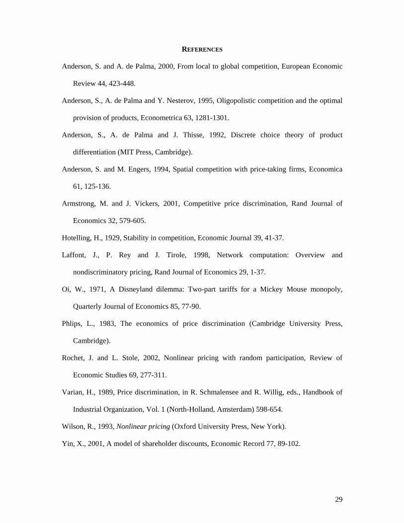
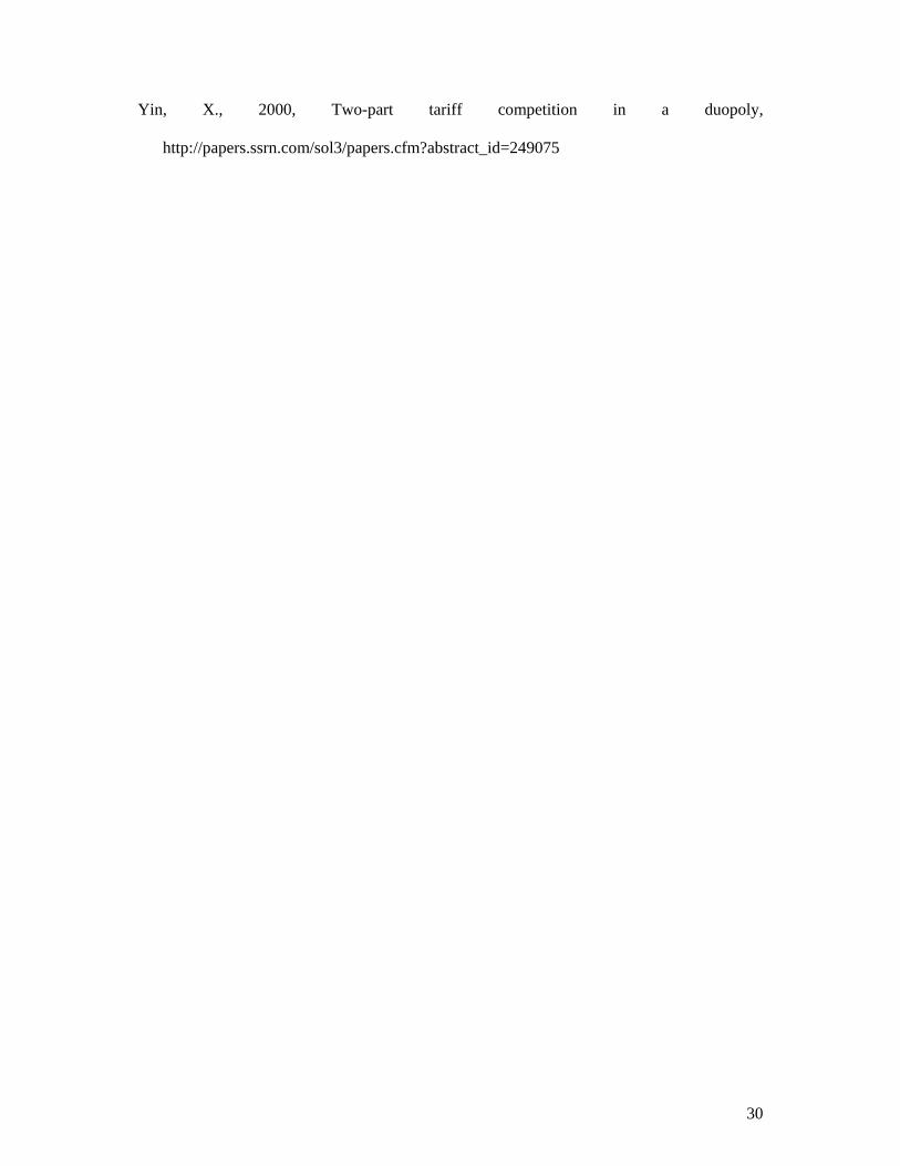
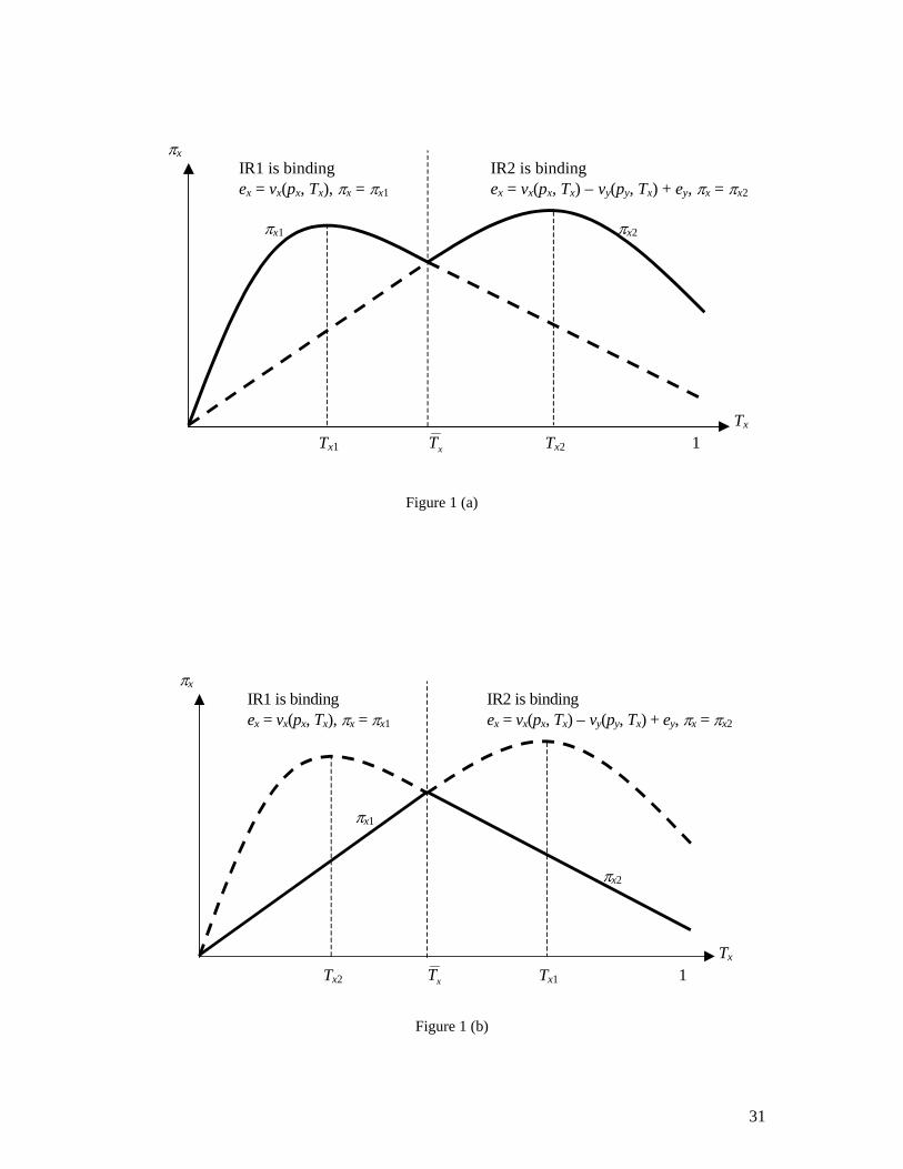
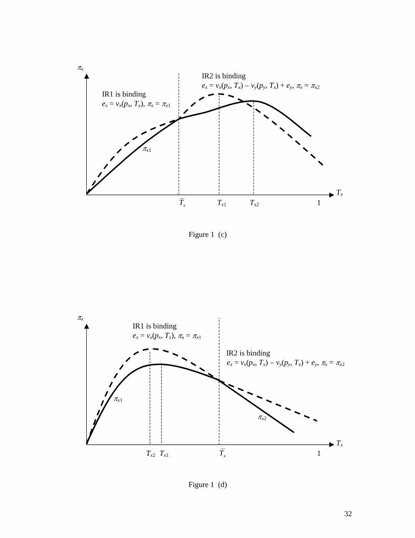
(px, Tx), to maximize its profits. Substituting (1) into (3), we can see from Figure 1 (the solid

lines) that given firm y’s tariffs, the profit function of firm x is continuous but kinked at

xx TT = , so that7

⎩⎨⎧

≥−++−≡≤−+≡

=xxxxxxxyxyyxxxx

xxxxxxxxxxxx TTTpXcpTFeTpvTpv

TTTpXcpTFTpv if ),()()(]),(),([ if ),()()(),(

2

1

ππ

π (4)

On the segment πx = πx1 (excluding the point xx TT = ), IR1 is binding so the marginal

consumers of firm x and firm y are different (i.e., Tx < Ty). But on the segment πx = πx2, IR2

is binding so the two marginal consumers are the same person (i.e., Tx = Ty). To simplify

analysis, it is assumed that πx1 and πx2 are concave functions of Tx ∈ [0, 1].

INSERT FIGURE 1 (a) − (d) AROUND HERE

Taking the partial derivative of profit function (4) with respect to px yields the first-

order condition (FOC) for profit maximization,

–x(px, Tx)F(Tx) + X(px, Tx) + (px – cx)∂X(px, Tx)/∂px = 0. (5)

On the other hand, the partial derivative with respect to Tx leads to

7 If 1≥xT or 0≤xT , πx = πx1 or πx = πx2 on the whole interval Tx ∈ [0, 1] and the profit function has no kinks.

8

∂πx/∂Tx = F(Tx)∂vx(px, Tx)/∂Tx + [vx(px, Tx) + (px – cx)x(px, Tx)]f(Tx) if xx TT ≤ , (6)

∂πx/∂Tx = [∂vx(px, Tx)/∂Tx – ∂vy(py, Tx)/∂Tx]F(Tx) + [vx(px, Tx) – vy(py, Tx) + ey]f(Tx)

+ (px – cx)x(px, Tx)f(Tx) if xx TT ≥ . (7)

Since πx1 and πx2 are assumed to be concave, (6) and (7) have a zero point, Tx1 and Tx2,

respectively (see Figure 1). However, it is quite likely that Tx1 does not fall within the

interval (0, xT ) (see Figure 1 (b) and (c)) and Tx2 not within ( xT , 1) (see Figure 1 (b) and (d)).

Thus, given firm y’s decision, there are four possible configurations of profit functions,8 and

the possible candidates for firm x’s optimal marginal consumer are those who are located at

0, 1, Tx1, Tx2 or xT . A further comparison between profit values at these points can determine

the best response in the choice of marginal consumer. Since Tx = 1 or Tx = 0 implies that

either firm x or firm y exits from the market so that the industry becomes monopolistic, these

two trivial cases will be excluded from the analysis below.

To facilitate discussion, several definitions are introduced. A full-cover market

means that each consumer is served by some firm while in a partial-cover market some

consumers are not served by either firm. The equilibria of a full-cover market can be further

divided into two types: a full competition equilibrium where the IR1 constraints of both

goods are slack and a kinked equilibrium where the marginal consumer is at the kink of profit

function. From (5), the following proposition is immediate.

Proposition 1. When consumer preferences are differentiated à la Hotelling, equilibrium

marginal prices are equal to marginal cost if and only if the demand of the marginal

consumer is equal to the average demand, i.e., x(px, Tx) = X(px, Tx)/F(Tx).

8 But we can rule out the case of Figure 1 (a) for equilibrium because ∂πx/∂Tx on the left of xT is smaller than its

counterpart on the right of xT .

9

Proposition 1 shows that the condition for marginal cost pricing under two-part tariff

competition and under two-part tariff monopoly is the same (for the case of monopoly, see

Varian (1989)). This similarity between monopoly and duopoly is due to the lack of strategic

effects of price decisions in both market structures, given each firm’s market territory. The

condition that the demand of the marginal consumer equals the average demand is not a

knife-edge case. For instance, as long as the effect of horizontal preference parameter on

utility is additively separate from price, then x(px, Tx) = x(px) and x(px, Tx) = X(px, Tx)/F(Tx).

More generally, we have the following corollary.9

Corollary 1. When consumers’ marginal utilities are monotonic on the Hotelling line (i.e.,

∂2ux(x, τ)/∂τ∂x ≤ 0 and ∂2uy(y, τ)/∂τ∂y ≥ 0) or conditional demands are monotonic (i.e.,

∂2vx(px, τ)/∂τ∂px ≥ 0 and ∂2vy(py, τ)/∂τ∂py ≤ 0), firms set marginal prices equal to marginal

cost if and only if the taste parameter does not interact with quantity (i.e., the transportation

cost is a shopping cost).10

Armstrong and Vickers (2001), Laffont et al. (1998), and Rochet and Stole (2002)

show that the marginal price is (unconditionally) equal to marginal cost in full competition

equilibrium.11 In their models (like our example 1 below), there is no interaction between the

location parameter and the quantity (or quality in the Rochet-Stole model), i.e., the

transportation cost is a shopping cost. Consequently, all consumers of the same vertical type

9 I would like to thank Simon Anderson (the editor) for proposing this corollary.

10 It should be noticed that the monotonicity of marginal utility or conditional demand imposes a restriction on

the model. In our setting, utility is monotonic but we do not impose any assumption on marginal utility

elsewhere. Therefore, for any given price a consumer buying less (i.e., with lower marginal utility) is likely to

have greater utility relative to other consumers. The condition that the marginal demand equals the average

demand in Proposition 1 allows such non-monotonicity of demand.

11 The cost structure is more complicated in Laffont et al. (1998) because of charges between competing

networks. The marginal cost pricing rule holds if inter-firm charges are marginal cost based.

10

purchase the same amount of a good, if they decide to buy it, despite location differences. In

other words, the particular utility functions they adopt ensure the demand of the marginal

consumer to be equal to the average demand. However, divergence in the form of per-trip

transportation costs is a special case of horizontal preference differentiation. In Example 2

below, where the location parameter interacts with quantity, the demand of the marginal

consumer is smaller than the average demand and marginal cost pricing does not hold.

The welfare function is defined as the sum of consumers’ surplus and firm profits:

),()(),()()(),()(),(),,,(1

0 yyyyxxxxyT yx

T

xyxyx TpYcpTpXcpdfpvdfpvTTppWy

x −+−++= ∫∫ ττττττ

(8)

Since Proposition 1 gives the condition for marginal cost pricing, we focus on the welfare

effects of entry fees. The partial derivative of (8) with respect Tx is

∂W(px, py, Tx, Ty)/∂Tx = [vx(px, Tx) + (px – cx)x(px, Tx)]f(Tx), if Tx < Ty (9)

∂W(px, py, T, T)/∂T = [vx(px, T) – vy(py, T) + (px – cx)x(px, T) – (py – cy)y(py, T)]f(T).

if Tx = Ty= T (10)

Recalling (6), the value of (9) at the partial-cover equilibrium (px, py, Tx1, Ty1) is

∂W(px, py, Tx1, Ty1)/∂Tx = – F(Tx1)∂vx(px, Tx1)/∂Tx > 0 ,

which implies that social welfare can be improved if each firm lowers the entry fee and

extends their market coverage. Moreover, evaluating (10) at the full-cover equilibrium we

find that it is not equal to zero in general, which implies that full-cover equilibrium entry fees

are generally not socially optimal. It should be noticed that the absolute values of the entry

fees are not critical to the social optimum when the market is fully covered because entry fees

only transfer wealth from consumers to producers as long as the marginal prices and the

marginal consumer are given. Rather the relative magnitude of the two entry fees plays a

central role since it determines the marginal consumer. Market equilibrium does not

maximize social welfare when the marginal consumer differs from the one determined by the

11

social optimum. However, in a symmetric setting, we have cx = cy and vx(p, T) = vy(p, 1 − T).

A symmetric equilibrium implies both firms set the same marginal price and entry fee and

have the same market size; i.e., px = py, ex = ey and Tx = 1 – Ty. Furthermore, we have Tx = Ty

= ½ in a symmetric full-cover equilibrium. Thus, from (10) we have ∂W/T = 0 at a

symmetric full-cover equilibrium, which implies the location of the marginal consumer

maximizes social welfare and in turn the entry fee is socially optimal. The welfare analysis

results are summarized in the following proposition.

Proposition 2. (i) The equilibrium marginal price of each good under two-part tariff

competition maximizes social welfare if and only if the demand of the marginal consumer is

equal to the average demand.

(ii) If two-part tariff competition leads to a partial-cover equilibrium, the market size

is too small and entry fees are too high relative to the welfare optimum.

(iii) A full-cover equilibrium generally does not result in optimal entry fees. But in a

symmetric full-cover equilibrium, the location of the marginal consumer and entry fees are

socially optimal.

Part (ii) of the proposition resembles the conclusion obtained in monopoly (see

Varian, 1989). This is not surprising because duopolistic firms in a partial-cover market are

local monopolists in their market ranges. Recalling that entry fees are only a wealth transfer

from consumers to producers and do not affect social welfare given the marginal prices and

marginal consumer, the symmetric full-cover equilibrium in (iii) plus marginal cost pricing is

only one of (infinitely) many social optima. The condition of symmetric equilibrium is

important to the conclusion in (iii). As Example 1 below shows, two firms in a kinked

equilibrium are likely to charge different entry fees within a symmetric setting. In that case

reducing the higher entry fee to allow consumers to purchase from the closer firm can

obviously save transportation costs and improve social welfare.

12

Another welfare implication of this model is that the partial-cover equilibrium and

symmetric kinked equilibrium maximize joint profits; that is the duopolistic competition

yields the same outcome as two-part tariff cartelization (for the proof, see the working paper

Yin, 2000). The intuition behind the similarity is straightforward. In the partial-cover

equilibrium both firms operate in their monopoly ranges and one firm’s tariffs do not affect

the demand for the other firm’s product. Thus, the outcome of two local monopolists is

equivalent to that of a single cartel. In the kinked equilibrium, the symmetry induces the

duopoly to select the same marginal consumer regardless of being imperfectly competitive or

collusive.12 When profit functions reach a maximum at the kinked point, competition

actually makes firms stick to the strategy of setting the entry fee equal to the marginal

consumer’s surplus in response to a range of the rival firm’s entry fee. So, imperfectly

competitive firms in equilibrium charge the same entry fee as the cartel does.

2.2) Comparison with Uniform Pricing

Linear prices can be considered as a special case of two-part tariffs where the entry

fees are restricted to zero. The marginal consumer under this pricing regime is characterized

by

vx(px, Tx) = max{vy(py, Tx), 0}.

This condition determines Tx as a function of px, given py. The derivative of Tx with respect

to px is

⎩⎨⎧

≥∂∂−∂∂≤∂∂

=0),( if]),(),([),( 0),( if]),([),(

xyyxxyyxxxxxx

xyyxxxxxx

x

x

TpvTTpvTTpvTpxTpvTTpvTpx

dpdT

(11)

Given py, let xT = argt{vy(py, t) = 0} be the marginal consumer who is indifferent

between buying x and buying y and buying neither x nor y (i.e., both IR1 and IR2 are binding)

12 The FOCs for equilibrium marginal prices of competition and cartelization are identical in all circumstances.

13

and let 0),(arg == xxpx Tpvp . Then, profit πx = (px – cx)X(px, Tx) is kinked at px = xp and xT

is the marginal consumer at the kink. The first-order derivative of πx is equal to

∂πx/∂px = X(px, Tx) + (px – cx)∂X(px, Tx)/∂px + (px – cx)x(px, Tx)f(Tx)dTx/dpx. (12)

Evaluating dTx/dpx in (12) by the first or second equation in (11) and setting (12) and its

counterpart for firm y equal to zero, the solution generates the partial-cover equilibrium or

full competition equilibrium. Moreover, there is a kink equilibrium if (12) is positive on the

left of xp and negative on the right of xp . Comparing (12) with (5), it is clear that the

equilibrium price of uniform price competition can be either higher or lower than that of two-

part tariff competition. Without more detailed specifications of the model, it is impossible to

draw unambiguous conclusions on prices and welfare. However, the lemma below shows

that price is a good indicator of welfare performance, which is helpful in our welfare analysis

of two examples in the next section.

Lemma 1. In a symmetric full-cover equilibrium, two-part tariff competition yields greater

social welfare than uniform pricing if and only if it results in a lower marginal price,

provided the equilibrium marginal price of two-part tariff competition is not smaller than

marginal cost.

The intuition of the lemma is obvious. If the market is covered, the aggregate welfare

increases as social welfare (consumer surplus plus profit) obtained from the sales to each

consumer is improved, which can be achieved with a lower marginal prices provided it is not

below marginal cost.

3. TWO EXAMPLES OF HOTELLING PREFERENCES

This section presents two examples of Hotelling preferences. In both examples,

consumers are uniformly distributed on [0, 1] and two firms have the same marginal cost; i.e.,

14

cx = cy = c. The main difference between the two examples is their transportation costs,

which induces divergence in demand structure and equilibrium characteristics.

3.1) Example 1: Shopping Model

This example adopts a simple shopping model so that utility is of the form

ux(x, τ) = u(x) – tτ and uy(y, τ) = u(y) − t(1 − τ), a ≥ 0 (13)

where u(x) and u(y) are utilities of consuming goods x and y, respectively. The transportation

costs for a consumer located at τ to firm x and firm y are tτ and t(1 − τ), respectively, which

are independent of the amount shipped. This utility specification is similar to Armstrong and

Vickers (2001) and Rochet and Stole (2002) if vertical preferences in their models are

abstracted. It can also be considered as a simplified version of the model studied by Laffont

et al. (1998) when one network has free access to the other network. With specification (13)

the demand function is independent of a consumer’s location as long as consumers decide to

purchase, i.e., x(px, τ) = x(px),. Consequently, consumer surplus functions are

vx(px, t) = v(px) –tτ and vy(py, t) = v(py) − t(1 − τ).

Since the demand of the marginal consumer is equal to the average demand, the firms

price their products at their marginal costs in equilibrium. To simplify notation, write v(c) as

v in the analysis of entry fees below. Thus, t/v can be considered as a measure of product

differentiation and/or consumer diversity. Given marginal cost pricing, we can interpret the

model as if consumers have unit demand with reservation price v and the entry fee is the price

for one unit.13 With standard calculation (which is available upon request) it can be shown

that there are three types of equilibria depending on the parameters of the model:

(a) A unique full competition equilibrium ex = ey = t with marginal consumer Tx2 = Ty2 = ½

when t/v ∈ [0, 2/3).

13 I would like to thank two anonymous referees for pointing out this analogue.

15

(b) A continuum of kinked equilibria with ex + ey = 2v − t for all (ex, ey) ∈ [4/3v − t, 3/2v − t]

× [4/3v − t, 3/2v − t] when t/v ∈ [2/3, 1]. Any τ ∈ [v/3t, 1 − v/3t] can be the equilibrium

marginal consumer if t/v ∈ [2/3, 5/6], and any τ ∈ [1 − v/2t, v/2t] is the equilibrium

marginal consumer if t/v ∈ [5/6, 1].

The symmetric kinked equilibrium is ex = ey = v − t/2 where the marginal consumer is

located at 2/1=T .

(c) A unique partial-cover equilibrium ex = ey = v/2 with marginal consumers Tx1 = v/2t and

Ty1 = 1 − v/2t when t/v ∈ (1, +∞).

These results show that as t/v increases, the equilibrium moves from the full competition

equilibrium to one of kinked equilibria and then to the partial-cover equilibrium. There are

three interesting observations about entry fees. The first is that equilibrium entry fees tend to

zero as t tends to zero. This demonstrates that if consumers are homogenous firms cannot

charge two-part tariffs. Second, the entry fees increase as v is larger (for the partial and

kinked equilibria) or t is larger (for the full competition equilibrium). This is obvious

because as consumers value the commodity higher, they are willing to pay more. On the

other hand, more diversified consumers implies firms have more market power and

consequently they can set a higher entry fee. Finally, the entry fees are strategic

complements in the full competition equilibrium range but they are strategic substitutes in the

kinked equilibrium range.

From now on, we focus on the symmetric equilibrium. In light of Proposition 2, we

have the corollary below.

Corollary 2. With the utility specifications in (13), two-part tariff competition results in a

socially optimal outcome if t/v ∈ (0, 1] but its entry fee is higher than the social optimal level

if t/v ∈ (1, +∞).

16

Turning to comparison with uniform pricing, it is possible that a symmetric

equilibrium under one tariff regime is fully covered but it turns out to be a partial-cover

equilibrium under the other tariff regime. Since the full-cover equilibrium is more

interesting, we consider such a demand and cost structure that results in full-cover

equilibrium in both tariff regimes. Recalling X(px, Tx) = x(px)Tx, (12) shows that the

symmetric full-cover equilibrium price under uniform pricing, pu, is characterized by

x(pu) + (pu – c)dx(pu)/dp – (pu – c)x2(pu)/t = 0 (14)

or

.0)()(2)()()(,0)()()()()(

2

2

<−−−+>−−−+tpxcpdppdxcppx

tpxcpdppdxcppxuuuuu

uuuuu

. (15)

Proposition 3. Assume consumers have the utility functions in (13). In comparison with

uniform price competition, two-part tariff competition results in a lower marginal price but

higher profits and social welfare in symmetric full-cover equilibrium. The aggregate net

consumer surplus is smaller if two-part tariff competition leads to a kinked equilibrium or if

the demand function x(p) is concave or if x(p) is convex but dx(c)/dp ≥ 2dx(pu)/dp.

The results regarding profits and social welfare in Proposition 3 are similar to those of

Armstrong and Vickers (2001) except for our inclusion of the kinked equilibrium. The result

on consumer surplus is slightly different. Although they do not explicitly spell out the

condition for their conclusion (Corollary 1, Armstrong and Vickers, 2001), an implicit

presumption in their analysis is that the profit function is concave in utility. While the

conditions specified in Proposition 3 and assumed by Armstrong and Vickers are moderate, it

seems unlikely to obtain an unambiguous conclusion on the relative magnitude of consumer

surplus without these conditions. From the proof of Proposition 3 it is not difficult to see that

two-part tariff competition (in full competition equilibrium) leads to greater aggregate net

consumer surplus than uniform pricing if v(pu) < v/3.

17

Monopolistic two-part tariffs definitely make the marginal consumer worse off in

contrast to uniform pricing since the monopolistic entry fee drives his surplus to zero (see

Phlips, 1982, Wilson, 1993 and Yin, 2001). However, the marginal consumer is likely to be

better off in two-part tariff duopoly than in uniform price duopoly. In this example, the

marginal consumer’s net surplus under the two-part tariff regime is v – 3t/2 if t/v ≤ 2/3 while

the surplus under the uniform pricing regime is v(pu) − t/2. Thus, if v(pu) < v/3, the two-part

tariff makes the marginal consumer better off.

3.2) Example 2: Shipping Model with Linear Demand

Suppose now that the transportation cost is proportionate to the distance and amount

shipped. More specifically, the utility function is assumed to be

ux(x, τ) = (b − x/2)x − δxτ, uy(y, τ) = (b − y/2)y − δy(1 − τ), (16)

where (b − x/2)x and (b − y/2)y are, respectively, the utilities from the consumption of the x-

good and the y-good by the consumer located at τ, and δxτ and δy(1 − τ) are his shipping

costs. Thus, the demands for goods x and y by the consumer located at τ, respectively, are

x(px, τ) = b – px − δτ and y(py, τ) = b – py − δ(1 − τ). (17)

To ensure the example is meaningful, it is assumed that b > c. For consumers who buy the x-

good (y-good), the larger is τ, the smaller (larger) is demand; that is, the quantity demanded is

determined not only by the price but also the location. Aggregate demand is

X(px, Tx) = τδτ dpbxT

x∫ −−0

)( = (b – px − δTx/2)Tx. (18)

The consumer surplus functions are

vx(px, τ) = (b – px − δτ)2/2 and vy(py, τ) = [b – py − δ(1 − τ)]2/2. (19)

Proposition 4. For the specification of Example 2, there is a unique symmetric partial-

cover equilibrium px = py = (b + 4c)/5 > c, Tx = 2(b –c)/5δ, Ty = 1 − 2(b –c)/5δ and ex = ey =

18

2(b – c)2/25 when (b – c) < 5δ/4. If (b – c) ≥ 5δ/4, the market is fully covered and symmetric

equilibrium marginal prices are px = py = c + δ/4. For 5δ/4 ≤ (b – c) < 9δ/4, the symmetric

equilibrium rests at the kink with entry fees ex = ey = (b − c − 3δ/4)2/2. For (b – c) ≥ 9δ/4, a

symmetric full competition equilibrium obtains with entry fees ex = ey = 3δ(b − c − 3δ/4)/4.

For uniform pricing, recalling (11)-(12) and (17)-(19), the symmetric full competition

equilibrium price pu is determined by

(b – pu − δTx/2)Tx – (pu – c){Tx + (b – pu − δTx)2/[b – pu − δTx + b – pu − δ(1 − Tx)]δ} = 0.

Since Tx = ½, it leads to the solution

⎥⎦⎤

⎢⎣⎡ −++−++−++= )4/2/(4)2/3(2/3 22

21 δδδδδ cbcbcbcbpu .

On the other hand, consider the FOC for partial-cover equilibrium,

(b – p − δTx/2)Tx – (p – c){Tx + (b – p − δTx)2/(b – p − δTx) = 0.

Setting Tx = ½, we obtain

⎥⎦⎤

⎢⎣⎡ −+−++−++= )4/2(8)22(22 22

41# δδδδ bcbcbcbp .

So, if the kinked equilibrium exists, the symmetric equilibrium price is greater than p# but

smaller than pu. The results of a comparison between two-part tariffs and linear pricing in

symmetric full-cover equilibrium are given below.

Proposition 5. With demand functions (17), two-part tariff competition leads to a lower

marginal price and aggregate net consumer surplus, but higher industry profits and social

welfare than uniform price competition.

4. Two-Part Tariff Competition with Logit Demand

4.1) The Model and Equilibrium

A feature of Hotelling preferences is that each firm either competes with the outside

choice (in a partial-cover equilibrium) or competes with the other firm’s product (in a full-

19

cover equilibrium). It excludes the possibility that a firm competes with the other firm at the

same time as it competes with the outside choice. To account for this simultaneous

competition on two fronts, an alternative is to assume that the taste parameter τ is randomly

drawn from a population. When a consumer faces prices px and py and entry fees ex and ey, he

derives the following consumer surplus, respectively, through the consumption of the x-, y- or

z- (outside) good:

vx(px, τ) = vx(px) + τx, vy(py, τ) = vy(py) + τy, vz(τ) = vz + τz.

In these equations, vx(px), vy(py) and vz are nonstochastic and reflect the population’s tastes14

and τx, τy and τz are stochastic and reflect the idiosyncrasies of this individual’s tastes for

goods x, y and z. Similar to the Hotelling model, individual rationality conditions, vx(px, τ) –

ex ≥ vz(τ) and vx(px, τ) – ex ≥ vy(py, τ) – ey, must hold for the x-good to be attractive to

consumer τ. But consumers steadily leave the x-good market as ex rises so that there are no

kinks in the demand function. To obtain logit demand functions, it is assumed that τi (i = x, y,

z) are i.i.d and follow the double exponential distribution with mean zero and variance σ2π2/6

so that the cumulative distribution function is

F(ω) =exp{−[exp−(γ + ω/σ)]},

where γ is Euler’s constant and σ is a positive constant. It can be shown (see, for example,

Anderson et al. (1992) Chapter 2) that the fractions of consumers, who choose the x-, y- or z-

good, respectively, are

∑ =−+

−=

yxj jjjz

iiii epvv

epvS

,]/))(exp[()/exp(

]/))(exp[(σσ

σ, i = x, y,

∑ =−+

=yxj jjjz

zz epvv

vS,

]/))(exp[()/exp()/exp(

σσσ . (20)

14 If the utility of consuming good x is ux(x), then vx(px) = maxx{ux(x) − pxx}.

20

Thus, the demand functions for the x-good and y-good are xSx and ySy, respectively, where

each consumer’s demand, x or y, is constant across consumers who decide to buy, and can be

obtained by Roy’s identity. As (20) illustrates there are always some consumers who

purchase neither good x nor good y when vz is a finite constant. But no consumers purchase z

and the market is fully covered if vz → −∞.

Firm x’s profit function can be written as15

πx = exSx + (px – cx)x(px)Sx.

Its partial derivatives with respect to px and ex yield the following FOCs:

x(px) + (px – cx)dx(px)/dpx – [ex + (px – cx)x(px)](1 − Sx)x(px)σ−1 = 0, (21)

1 – [ex + (px – cx)x(px)](1 − Sx)σ−1 = 0. (22)

Define the symmetric case as in Sections 2 and 3 so that vx(⋅) = vy(⋅) = v(⋅) and cx = cy = c and

let v(c) ≡ v. From (21) and (22), we can immediately obtain the proposition below.

Proposition 6. In the logit model, two-part tariff competition leads to marginal cost pricing

in equilibrium and in the symmetric case the equilibrium entry fee, e, can be characterized by

e = σ/(1 − Sx) =⎭⎬⎫

⎩⎨⎧

−+−

+]/)exp[()/exp(

]/)exp[(1σσ

σσevv

ev

z

. (23)

Moreover de/dvz < 0 and e = 2σ when vz → −∞.

The result de/dvz < 0 is intuitive: when the outside option becomes more attractive

(i.e., vz is larger) the firms have less market power so that they have to lower entry fees to

attract consumers. At the extreme (i.e., vz → −∞), consumers do not purchase the outside

option and the firms can set the highest entry fee e = 2σ.

15 Note that Sx is a function of px, py, ex, ey. To simplify notation, these variables are dropped in the expressions.

21

A consumer purchasing good x, y or z has net consumer surplus vx(px) + τx − ex, vy(py)

+ τy − ey or vz + τz, respectively. Following the same proof in Anderson et al. (1992, Chapter

2), it can be shown that the aggregate net consumer surplus under the two-part tariff regime is

⎭⎬⎫

⎩⎨⎧ −+= ∑ = yxj jjjz epvvCS

,]/))(exp[()/exp(ln σσσ .

By definition the welfare function is W = CS + (πx + πy). Since two-part tariff competition

leads to marginal cost pricing, we need only investigate the welfare effects of the entry fee:

∂W/∂ex = −Sx + Sx{1 − [ex + (px – cx)x](1 − Sx)σ−1 + [ey + (py – cy)y]Syσ−1}.

Substituting the marginal price and entry fee into the symmetric equilibrium yields

∂W/∂ex = Sx(eySyσ−1 − 1) < 0.

However, if there is no outside option (i.e., vz → −∞), eySy = σ by (23), so ∂W/∂ex = 0.

Proposition 7. The symmetric equilibrium of two-part tariff competition with logit demand

leads to a socially optimal marginal price but the entry fee is too high and the market

coverage too small.16 If there is no outside option, the equilibrium is socially optimal.

4.2) Comparison with Uniform Pricing

In uniform price competition, the equilibrium price, pxu, is characterized by

x(pxu) + (px

u – cx)dx(pxu)/dpx – (px

u – cx)x(pxu)(1 − Sx)x(px

u)σ−1 = 0, (24)

which implies above-marginal-cost pricing. There is an unambiguous conclusion for the

comparison between the welfare outcomes of two-part tariffs and uniform pricing if there is

no outside option. However, with an outside option, only aggregate net consumer surplus

and profits can be unambiguously compared.

Proposition 8. If x(p) and y(p) are log-concave, two-part tariff competition results in a

smaller market coverage, less aggregate net consumer surplus and more profits than uniform

16 When vz is finite the welfare maximizing entry fee is ex = 0 since ∂W/∂ex < 0 for all positive ex.

22

price competition in symmetric equilibrium. If there is no outside option, it also yields

greater social welfare.

5. Closing Discussion

The utility functions in the logit model are similar to those in Example 1 in the sense

that preference divergence is an additive term in the utility functions and there is no

interaction between the preference parameter and the quantity demanded. This similarity

implies that consumers in both settings have identical demand functions if they buy a

product, which in turn results in marginal cost pricing. Moreover, both settings show that the

symmetric full-cover equilibrium is socially optimal but the partial-cover equilibrium is not.

On the other hand, the random distribution of consumer preferences of the logit model makes

it differ substantially from Example 1. There is no systematic relationship between the tastes

of any two consumers in the logit model. Consequently, firms do not have exclusive market

territories and cannot behave as local monopolists.

For applications, it is hard to say whether the assumption of Hotelling preferences is

better than the assumption of logit demand or not. Hotelling preferences may be appealing

for industries such as wired telephone services where the market is completely covered and

variations in tariffs only make consumers switch between firms. On the other hand, logit

demand may be more plausible for other situations such as luxury club memberships where a

reduction in price and/or entry fee attracts consumers from other suppliers as well as new

customers. The most appropriate assumption for a particular industry or market is an

empirical question.

23

Appendix

Proof of Corollary 1

Since px = ∂ux(x, τ)/∂x, the demand function is independent of τ when τ does not

interact with x in the utility function. So, x(px, Tx) = X(px, Tx)/F(Tx).

On the other hand, ∂2ux(x, τ)/∂τ∂x ≤ 0 or ∂2vx(px, τ)/∂τ∂px ≥ 0 implies ∂x(px, τ)/∂τ ≤ 0.

It is obvious that the demand function is independent of τ when ∂x(px, τ)/∂τ ≤ 0 and x(px, Tx)

= X(px, Tx)/F(Tx). Hence, there is no interaction between τ and x in the utility function.

Proof of Lemma 1

Let c be the marginal cost and p the equilibrium marginal price in the symmetric case.

Superscripts t and u indicate two-part tariffs and uniform pricing, respectively. Then

( tW − uW )/2 = ∫ −5.0

0)],(),([ τττ dpvpv u

xt

x + (pt − c)X(pt, 0.5) − (pu − c)X(pu, 0.5)

= ∫u

t

p

pdppX )5.0,( − (pu − pt)X(pu, 0.5) + (pt − c)[X(pt, 0.5) − X(pu, 0.5)].

Because X(⋅, 0.5) is downward sloping and pt >c, tW > uW if and only if pt < pu.

Proof of Proposition 3

From (14)-(15), pu > c is obvious. By Lemma 1 the conclusion of total welfare is immediate.

Let CS and Π be aggregate net consumer surplus and industry profits, respectively. Then,

⎩⎨⎧

≤≤−<<

=1/2/3 if2/

2/3/0 ifvttv

vtttΠ ,

uΠ = (pu – c)x(pu).

Recalling (14)-(15) and dx(pu)/dp < 0, we have uΠ = (pu – c)x(pu) < a. Moreover, v(pu) ≥ t/2

since all consumers participate in the market. Thus, v − t/2 = v(pu) + ∫up

cdppx )( − t/2 > (pu –

24

c)x(pu). So, tu ΠΠ < . On the other hand, uCS − tCS = t − ∫up

cdppx )( . Equations (14) and

(15) imply that

t ≥ (pu – c)x2(pu)/[x(pu) + (pu – c)dx(pu)/dp].

When x(p) is concave, we have

∫up

cdppx )( < (pu – c)x(c) ≤ (pu – c)[x(pu) − (pu – c)dx(pu)/dp],

A direct comparison shows t ≥ ∫up

cdppx )( . When x(p) is convex, we obtain

∫up

cdppx )( ≤ (pu – c)[x(pu) + x(c)]/2 = (pu – c)[2x(pu) − (pu – c)dx(p′)/dp]/2

≤ (pu – c)[x(pu) − (pu – c)2dx(pu)/dp].

where p′∈ (c, pu). In the last inequality, dx(p′)/dp ≥ dx(c)/dp ≥ 2dx(pu)/dp is applied.

Proof of Proposition 4

Substituting (17) and (18) into (5) yields px = c + δTx/2. Similarly, setting (6) equal to

zero yields Tx1 = (b + px – 2c)/3δ. Solving these two equations and their counterparts for firm

y yields a unique symmetric partial-cover equilibrium px = py = (b + 4c)/5 > c, Tx = 2(b –

c)/5δ, Ty = 1 − 2(b –c)/5δ and ex = ey = 2(b –c)2/25 when (b – c) < 5δ/4.

The above proof also shows that there is no partial-cover symmetric equilibrium when

(b – c) ≥ 5δ/4. Since Tx = Ty = ½ in a full-cover symmetric equilibrium, the equilibrium

marginal prices are px = py = c + δ/4. Substituting these values into (7) and setting it equal to

zero yield symmetric-full-competition-equilibrium entry fees ex = ey = 3δ(b − c − 3δ/4)/4.

Recalling ey ≤ v(c + δ/4, 1/2) = (b − c − 3δ/4)2/2, the condition for the existence of the

symmetric full-competition equilibrium is (b – c) ≥ 9δ/4. For 5δ/4 ≤ (b – c) < 9δ/4,

substituting px = py = c + δ/4 and Ty = ½ into (6) and (7), we obtain

25

021|−=∂

∂

xTx

x

Tπ

= (b − c − 3δ/4)(b − c − 5δ/4)/2 ≥ 0, 02

1|+=∂

∂

xTx

x

Tπ

= ey − 3δ (b − c − 3δ/4)/4< 0.

So, the symmetric full-cover equilibrium is at the kink and equilibrium entry fees are ex = ey =

(b − c − 3δ/4)2/2.

Proof of Proposition 5

First, consider the case where uniform pricing results in a symmetric full competition

equilibrium. Define )4/2/(4)2/3( 22 δδδδ −++−++≡∆ cbcbcb , then pu > pt ⇔ (b – c

+ δ) > ∆ ⇔ (b – c) > 3δ/4. Since a full-cover equilibrium of two-part tariff completion

implies (b – c) ≥ 5δ/4, pu > pt is true. Recalling Lemma 1 we have Wt > Wu. Note, the full

competition equilibrium results in higher entry fees than the kinked equilibrium under two-

part tariffs and ∫5.0

0),(2 ττ dpv = (b − p)(b − p − δ/2)/2 +δ2/24. Routine calculation shows,

tCS ≤ ∫ +5.0

0),4/(2 ττδ dcv − 3δ(b − c − 3δ/4)/4 = (b − c − 7δ/4)(b − c − 3δ/4)/2 +δ2/24,

uCS = ∫5.0

0),(2 ττ dpv u = (b − c − 3δ/2 + ∆)(b − c − 5δ/2+ ∆)/8 +δ2/24.

Because ∆ > b − c − δ/2, it is immediately apparent that tCS < uCS .

tΠ = e + 2(pt – c)X(pt, ½) ≥ δ(b − c − 11δ/16),

uΠ = 2(pu – c)X(pu, ½)/2 =δ(b − c −δ/4) − 7δ(b − c + 3δ/2 − ∆)/8.

tΠ − uΠ > 0 ⇔ 7δ(b − c + 2δ − ∆)/8 > 0 ⇔ (b – c + 2δ) > ∆. Since we have shown

(b – c + δ) > ∆, it is true that tΠ > uΠ .

If uniform pricing leads to a symmetric kinked equilibrium, then the equilibrium price

is between p# and pu. With the similar calculation, we can prove p# ≥ pt and the proposition

also holds when the equilibrium of uniform price competition rests on the kink.

26

Proof of Proposition 6

Marginal cost pricing is clear by substituting (22) into (21). The first equality in (23)

is obtained from (22) by setting px = cx and the second by substituting symmetric (20) into

σ/(1 − Sx). It is obvious that

e −⎭⎬⎫

⎩⎨⎧

−+−

+]/)exp[()/exp(

]/)exp[(1σσ

σσevv

ev

z

is continuous and increasing in e. Moreover, it is positive when e = 0 and tends to −σ when e

tends to positive infinity, so (23) has a unique positive solution.

Routine calculation shows that de/dvz < 0 and e = 2σ when vz → −∞.

Proof of Proposition 8

Let S be a firm’s market share in a symmetric equilibrium. Then,

uS = exp[v(pu)/σ]/{exp(vz/σ) + 2exp[v(pu)/σ]},

tS = exp[(v − e)/σ]/{exp(vz/σ) + 2exp[(v − e)/σ]},

uCS = σln{exp(vz/σ) + 2exp[v(pu)/σ]}, tCS = σln{exp(vz/σ) + 2exp[(v − e)/σ]},

uΠ = 2(pu − c)x(pu) uS , tΠ = 2e tS .

First, let us suppose no outside option (vz →−∞). Then, uS = tS = ½ and uCS −

tCS > e − (pu − c)x(c). Recalling e = 2σ and applying (24), we have uCS − tCS > 2σ −

2σ[x(pu) + (pu − c)x′(pu)]x(c)/x2(pu). By the log-concavity of the demand function,

x(pu) − x(c) = (pu − c)x′( p̂ ) ≥ (pu − c)x′(pu)x( p̂ )/x(pu) > (pu − c)x′(pu)x(c)/x(pu),

where p̂ ∈ (c, pu). Therefore, uCS − tCS > 2σ − 2σ{x(c)/x(pu) + [x(pu) − x(c)]/x(pu)]} = 0.

Recalling (21), uΠ = (pu − c)x(pu) = 2σ[x(pu) + (pu − c)x′(pu)]/x(pu) < 2σ = e = tΠ .

With fully covered markets, uW − tW = v(pu) + (pu − c)x(pu) − v < 0.

27

Now consider the case where the outside option exists. Note )( zu vCS and )( z

t vCS

are continuous functions of vz and )(−∞uCS > )(−∞tCS . Suppose that there is a finite

zv~ such that )~( zu vCS < )~( z

t vCS . Then, )( zu vCS − )( z

t vCS has at least one zero point. Let

zv̂ be the smallest zero point. We obtain )( zu vCS < )( z

t vCS for vz ∈( zv̂ , zv̂ + ε), where ε is a

sufficiently small positive constant. In turn, zzu vvCS d)(d = exp(vz/σ)/{exp(vz/σ) +

2exp[v(pu)/σ]} > exp(vz/σ)/{exp(vz/σ) + 2exp[(v − e)/σ]} = zzt vvCS d)(d for vz ∈( zv̂ , zv̂ + ε).

This implies )( zu vCS > )( z

t vCS on ∈( zv̂ , zv̂ + ε) and leads to a contradiction. Therefore, it

is impossible to have )( zu vCS < )( z

t vCS for all vz ∈(−∞, ∞).

Turning to the profit comparison, (21)-(22) show that in response to firm y’s tariffs

(py, ey), firm x chooses

ex = σ/(1 − Sx), (A1)

where

Sx = exp[(v − ex)/σ]/{exp(vz/σ) + exp[(v − ex)/σ] + exp( v /σ) } (A2)

and v ≡ v(py) − ey. In particular, let xe~ be the solution to (A1) when firm y charges tariffs

(pu, 0) and v = v(pu). Since firm x prefers to charge tariffs (c, xe~ ) resulting in profit xπ~

rather than to set (pu, 0) to yield profit 2uΠ , it implies that xπ~ > 2uΠ . When firm y sets

tariffs (c, e) and v = v − e, (21)-(22) show that firm x sets (c, e) to earn 2tΠ . From (A1)

and (A2),

vS

Sve x

x

x

dd

)1(dd

2−=

σ , 2)}/exp(]/)exp[()/{exp(

)/exp(dd)]/exp()/[exp(]/)exp[(

dd

σσσσ

σσσσ

vevv

vvevvev

vS

xz

xzx

x

+−+⎭⎬⎫

⎩⎨⎧ ++−−

= .

Solving these two equations, we obtain 0dd <vex and 0dd <vSx . Thus, as v falls from

v(pu) to v − e, profit increases from xπ~ to 2tΠ , which proves that 2tΠ > xπ~ > 2uΠ .

28

Acknowledgement

The author is most grateful to Simon Anderson (the editor), Mark Armstrong and two

anonymous referees for very constructive and detailed comments. He would also like to

thank Buly Cardak, Chongwoo Choe, Harry Clarke, Gillian Hewitson, David Prentice and

Robert Waschik for helpful discussions and comments.

29

REFERENCES

Anderson, S. and A. de Palma, 2000, From local to global competition, European Economic

Review 44, 423-448.

Anderson, S., A. de Palma and Y. Nesterov, 1995, Oligopolistic competition and the optimal

provision of products, Econometrica 63, 1281-1301.

Anderson, S., A. de Palma and J. Thisse, 1992, Discrete choice theory of product

differentiation (MIT Press, Cambridge).

Anderson, S. and M. Engers, 1994, Spatial competition with price-taking firms, Economica

61, 125-136.

Armstrong, M. and J. Vickers, 2001, Competitive price discrimination, Rand Journal of

Economics 32, 579-605.

Hotelling, H., 1929, Stability in competition, Economic Journal 39, 41-37.

Laffont, J., P. Rey and J. Tirole, 1998, Network computation: Overview and

nondiscriminatory pricing, Rand Journal of Economics 29, 1-37.

Oi, W., 1971, A Disneyland dilemma: Two-part tariffs for a Mickey Mouse monopoly,

Quarterly Journal of Economics 85, 77-90.

Phlips, L., 1983, The economics of price discrimination (Cambridge University Press,

Cambridge).

Rochet, J. and L. Stole, 2002, Nonlinear pricing with random participation, Review of

Economic Studies 69, 277-311.

Varian, H., 1989, Price discrimination, in R. Schmalensee and R. Willig, eds., Handbook of

Industrial Organization, Vol. 1 (North-Holland, Amsterdam) 598-654.

Wilson, R., 1993, Nonlinear pricing (Oxford University Press, New York).

Yin, X., 2001, A model of shareholder discounts, Economic Record 77, 89-102.

30

Yin, X., 2000, Two-part tariff competition in a duopoly,

http://papers.ssrn.com/sol3/papers.cfm?abstract_id=249075

31

πx IR1 is binding IR2 is binding ex = vx(px, Tx), πx = πx1 ex = vx(px, Tx) − vy(py, Tx) + ey, πx = πx2

πx1 πx2 Tx

Tx1 xT Tx2 1

Figure 1 (a)

πx IR1 is binding IR2 is binding ex = vx(px, Tx), πx = πx1 ex = vx(px, Tx) − vy(py, Tx) + ey, πx = πx2

πx1 πx2 Tx

Tx2 xT Tx1 1

Figure 1 (b)

32

πx IR2 is binding ex = vx(px, Tx) − vy(py, Tx) + ey, πx = πx2 IR1 is binding

ex = vx(px, Tx), πx = πx1 πx1 Tx

xT Tx1 Tx2 1

Figure 1 (c)

πx IR1 is binding ex = vx(px, Tx), πx = πx1

IR2 is binding ex = vx(px, Tx) − vy(py, Tx) + ey, πx = πx2 πx1

πx2 Tx

Tx2 Tx1 xT 1

Figure 1 (d)