Embed Size (px)
Citation preview

introduction first problem
two optimization problems in physiology
michele piana
the MIDA groupdipartimento di matematica universita di genova and CNR-SPIN, genova
sestri levante, september 9 2014
introduction first problem
credits
thanks to the ’med-lab’ and ’neuro-lab at the MIDA group...
sara garbarino
franco caviglia
fabrice delbary
annalisa perasso
cristina campi
annalisa pascarella
riccardo aramini
anna maria massone
alberto sorrentino
valentina vivaldi
sara sommariva
cristian toraci
gianvittorio luria
...and to some external collaborators
gianmario sambuceti (IRCCS san martino IST and universita di genova)
cecilia marini (CNR IBFM, milano)
lauri parkkonen (aalto university)
maureen clerc (INRIA, sophia antipolis)
thomas serre (brown university)

introduction first problem
first problem

introduction first problem
FDG-PET
FDG is a glucose analog that allows trackingglucose metabolism
glucose consumption by malignant cells tendsto increase the FDG uptake
standard uptake value (SUV) depends on
the aggressiveness of cells
the amount of FDG at disposal in theenvironment
co-morbidities: what if cancer proliferates in adiabetic organism?

introduction first problem
compartmental analysis
concept:
compartment: homogeneous functional behavior (focused on tracer metabolism)
input for kinetics: FDG concentration in blood
kinetics’ descriptor: exchange coefficients
data: FDG (micro)-PET images
mathematical model:
the kinetic input is modeled by an input function which is obtained by fitting ROIsover the left ventricle
the compartmental model is a system of ODEs
the exchange coefficients are modeled by a vector in RN+
the data is a weighted sum of concentrations in the different compartments as afunction of time
introduction first problem
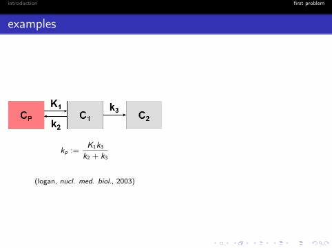
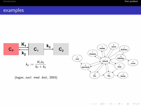
examples
kp :=K1k3
k2 + k3
(logan, nucl. med. biol., 2003)
introduction first problem
examples
kp :=K1k3
k2 + k3
(logan, nucl. med. biol., 2003)
introduction first problem
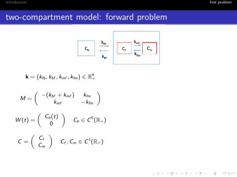
two-compartment model: forward problem
k = (kfb, kbf , kmf , kfm) ∈ R4+
M =
(−(kbf + kmf ) kfm
kmf −kfm
)
W (t) =
(Cb(t)
0
)Cb ∈ C 0(R+)
C =
(Cf
Cm
)Cf ,Cm ∈ C 1(R+)
C = MC + kfbW
C(t) = kfb
∫ t
0
Cb(u) exp((t − u)M)e1du
introduction first problem
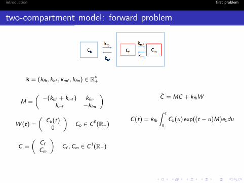
two-compartment model: forward problem
k = (kfb, kbf , kmf , kfm) ∈ R4+
M =
(−(kbf + kmf ) kfm
kmf −kfm
)
W (t) =
(Cb(t)
0
)Cb ∈ C 0(R+)
C =
(Cf
Cm
)Cf ,Cm ∈ C 1(R+)
C = MC + kfbW
C(t) = kfb
∫ t
0
Cb(u) exp((t − u)M)e1du
introduction first problem
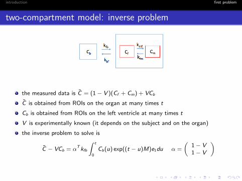
two-compartment model: inverse problem
the measured data is C = (1− V )(Cf + Cm) + VCb
C is obtained from ROIs on the organ at many times t
Cb is obtained from ROIs on the left ventricle at many times t
V is experimentally known (it depends on the subject and on the organ)
the inverse problem to solve is
C − VCb = αTkfb
∫ t
0
Cb(u) exp((t − u)M)e1du α =
(1− V1− V
)

introduction first problem
uniqueness
(delbary, garbarino and vivaldi, inverse problems, in preparation)
theorem: given k and k′ solutions of the equation
C − VCb = αT kfb
∫ t
0Cb(u) exp((t − u)M)e1du α =
(1− V1− V
)such that k, k′ ∈ R4
+ \ 0 and V ∈ (0, 1), then k = k′.
Proof (sketch): computing the laplace transform of the equation leads to
αT (s −M′)−1e1 = αT (s −M)−1e1.
this impliesQ(s)
P(s)=
Q′(s)
P′(s)
where Q(s),P(s) are co-prime polynomials of degree 1 and 2, respectively. this impliesQ(s) = Q′(s) and P(s) = P′(s). this in turn implies k = k′

introduction first problem
inversion algorithm
C − VCb − αTkfb
∫ t
0
Cb(u) exp((t − u)M)e1du = 0 α =
(1− V1− V
)F : k→ αTkfb
∫ t
0
Cb(u) exp((t − u)M)e1du
newton scheme:
1 solve in h[dFdk
(k; h)
](t) = C − VCb − αT (kfb)
∫ t
0
Cb(u) exp((t − u)M)e1du
2
k = k + h
note: in order to assure stability a penalty term is added
introduction first problem
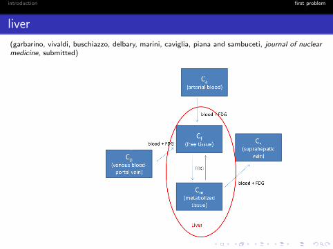
liver
(garbarino, vivaldi, buschiazzo, delbary, marini, caviglia, piana and sambuceti, journal of nuclearmedicine, submitted)
introduction first problem
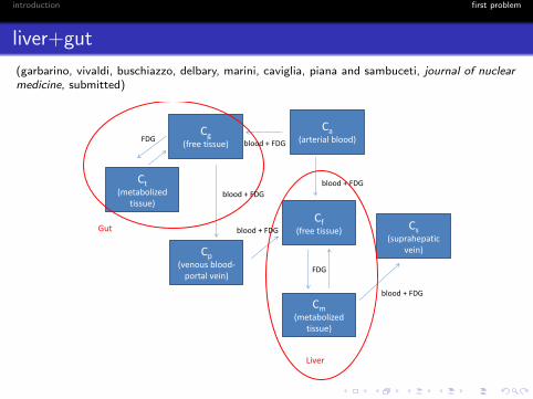
liver+gut
(garbarino, vivaldi, buschiazzo, delbary, marini, caviglia, piana and sambuceti, journal of nuclearmedicine, submitted)
Ca (arterial blood)
Cm (metabolized
tissue)
Cf (free tissue)
Liver
blood + FDG
FDG
Cp (venous blood-
portal vein)
Cs (suprahepatic
vein)
blood + FDG
Ct (metabolized
tissue)
Cg (free tissue)
FDG
Gut
blood + FDG
blood + FDG
blood + FDG
introduction first problem
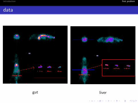
data
gut liver
introduction first problem
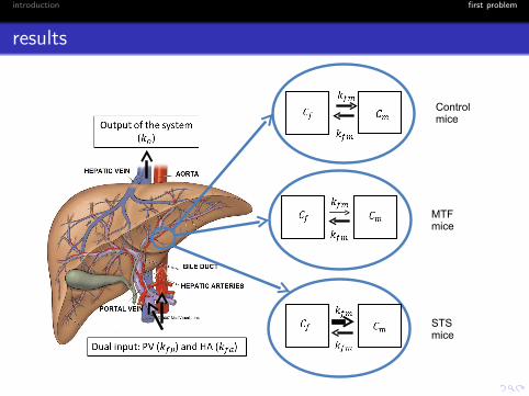
results
Control mice
MTF mice
STS mice

introduction first problem
second problem
introduction first problem
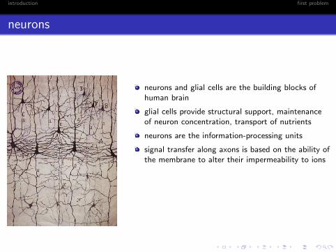
neurons
neurons and glial cells are the building blocks ofhuman brain
glial cells provide structural support, maintenanceof neuron concentration, transport of nutrients
neurons are the information-processing units
signal transfer along axons is based on the ability ofthe membrane to alter their impermeability to ions
introduction first problem
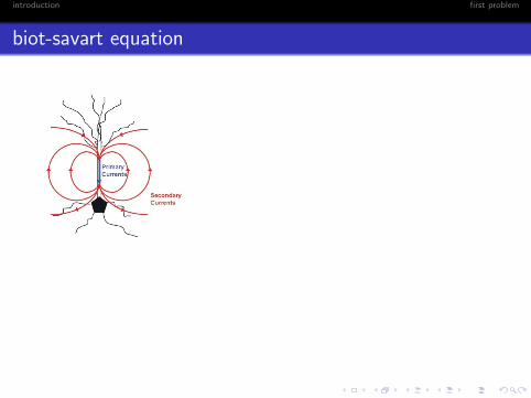
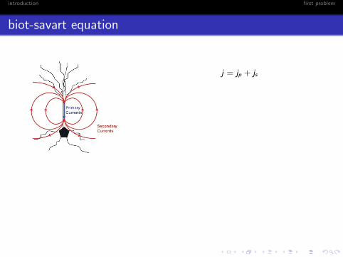
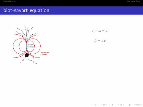
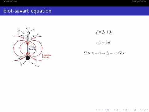
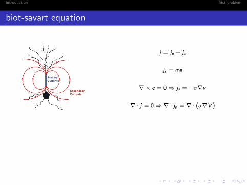
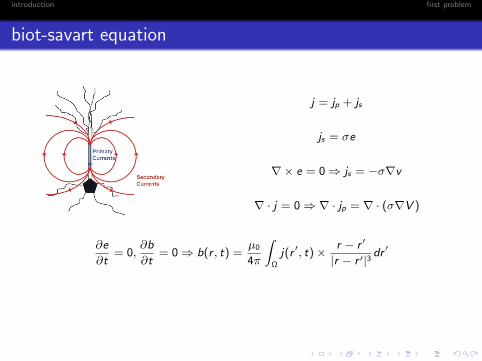
biot-savart equation
j = jp + js
js = σe
∇× e = 0⇒ js = −σ∇v
∇ · j = 0⇒ ∇ · jp = ∇ · (σ∇V )
∂e
∂t= 0,
∂b
∂t= 0⇒ b(r , t) =
µ0
4π
∫Ω
j(r ′, t)× r − r ′
|r − r ′|3 dr′
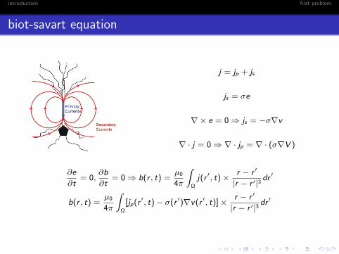
b(r , t) =µ0
4π
∫Ω
[jp(r ′, t)− σ(r ′)∇v(r ′, t)]× r − r ′
|r − r ′|3 dr′
introduction first problem
biot-savart equation
j = jp + js
js = σe
∇× e = 0⇒ js = −σ∇v
∇ · j = 0⇒ ∇ · jp = ∇ · (σ∇V )
∂e
∂t= 0,
∂b
∂t= 0⇒ b(r , t) =
µ0
4π
∫Ω
j(r ′, t)× r − r ′
|r − r ′|3 dr′
b(r , t) =µ0
4π
∫Ω
[jp(r ′, t)− σ(r ′)∇v(r ′, t)]× r − r ′
|r − r ′|3 dr′
introduction first problem
biot-savart equation
j = jp + js
js = σe
∇× e = 0⇒ js = −σ∇v
∇ · j = 0⇒ ∇ · jp = ∇ · (σ∇V )
∂e
∂t= 0,
∂b
∂t= 0⇒ b(r , t) =
µ0
4π
∫Ω
j(r ′, t)× r − r ′
|r − r ′|3 dr′
b(r , t) =µ0
4π
∫Ω
[jp(r ′, t)− σ(r ′)∇v(r ′, t)]× r − r ′
|r − r ′|3 dr′
introduction first problem
biot-savart equation
j = jp + js
js = σe
∇× e = 0⇒ js = −σ∇v
∇ · j = 0⇒ ∇ · jp = ∇ · (σ∇V )
∂e
∂t= 0,
∂b
∂t= 0⇒ b(r , t) =
µ0
4π
∫Ω
j(r ′, t)× r − r ′
|r − r ′|3 dr′
b(r , t) =µ0
4π
∫Ω
[jp(r ′, t)− σ(r ′)∇v(r ′, t)]× r − r ′
|r − r ′|3 dr′
introduction first problem
biot-savart equation
j = jp + js
js = σe
∇× e = 0⇒ js = −σ∇v
∇ · j = 0⇒ ∇ · jp = ∇ · (σ∇V )
∂e
∂t= 0,
∂b
∂t= 0⇒ b(r , t) =
µ0
4π
∫Ω
j(r ′, t)× r − r ′
|r − r ′|3 dr′
b(r , t) =µ0
4π
∫Ω
[jp(r ′, t)− σ(r ′)∇v(r ′, t)]× r − r ′
|r − r ′|3 dr′
introduction first problem
biot-savart equation
j = jp + js
js = σe
∇× e = 0⇒ js = −σ∇v
∇ · j = 0⇒ ∇ · jp = ∇ · (σ∇V )
∂e
∂t= 0,
∂b
∂t= 0⇒ b(r , t) =
µ0
4π
∫Ω
j(r ′, t)× r − r ′
|r − r ′|3 dr′
b(r , t) =µ0
4π
∫Ω
[jp(r ′, t)− σ(r ′)∇v(r ′, t)]× r − r ′
|r − r ′|3 dr′
introduction first problem
biot-savart equation
j = jp + js
js = σe
∇× e = 0⇒ js = −σ∇v
∇ · j = 0⇒ ∇ · jp = ∇ · (σ∇V )
∂e
∂t= 0,
∂b
∂t= 0⇒ b(r , t) =
µ0
4π
∫Ω
j(r ′, t)× r − r ′
|r − r ′|3 dr′
b(r , t) =µ0
4π
∫Ω
[jp(r ′, t)− σ(r ′)∇v(r ′, t)]× r − r ′
|r − r ′|3 dr′

introduction first problem
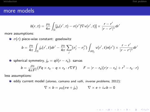
more models
b(r , t) =µ0
4π
∫Ω
[jp(r ′, t)− σ(r ′)∇v(r ′, t)]× r − r ′
|r − r ′|3 dr′
more assumptions:
σ(r) piece-wise constant: geselowitz
b =µ0
4π
∫Ω
jp(r ′, t)dr ′ − µ0
4π
∑j
(σ′j − σ′′j )
∫∂Ωj
v(r ′, t)n(r ′)× r − r ′
|r − r ′|3 dr′
spherical symmetry, jp = qδ(r − rq): sarvas
b =µ0
4πF 2(Fq × rq − q × rq · r∇F ) F = |r − rq|(r |r − rq|+ r 2 − rq · r)
less assumptions:
eddy current model (alonso, camano and valli, inverse problems, 2012):
∇× b = µ0(σe + jp) ∇× e + iωb = 0
full maxwell (albanese and monk, inverse problems, 2006):
∇× b − iωεµ0e = µ0(σe + jp) ∇× e + iωb = 0

introduction first problem
more models
b(r , t) =µ0
4π
∫Ω
[jp(r ′, t)− σ(r ′)∇v(r ′, t)]× r − r ′
|r − r ′|3 dr′
more assumptions:
σ(r) piece-wise constant: geselowitz
b =µ0
4π
∫Ω
jp(r ′, t)dr ′ − µ0
4π
∑j
(σ′j − σ′′j )
∫∂Ωj
v(r ′, t)n(r ′)× r − r ′
|r − r ′|3 dr′
spherical symmetry, jp = qδ(r − rq): sarvas
b =µ0
4πF 2(Fq × rq − q × rq · r∇F ) F = |r − rq|(r |r − rq|+ r 2 − rq · r)
less assumptions:
eddy current model (alonso, camano and valli, inverse problems, 2012):
∇× b = µ0(σe + jp) ∇× e + iωb = 0
full maxwell (albanese and monk, inverse problems, 2006):
∇× b − iωεµ0e = µ0(σe + jp) ∇× e + iωb = 0
introduction first problem
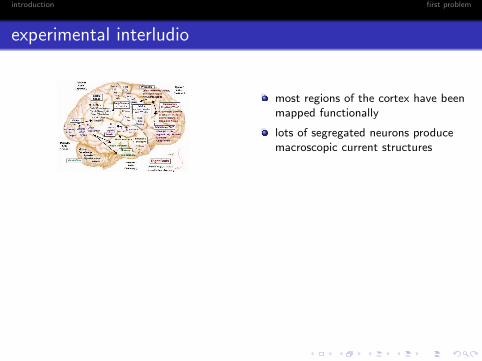
experimental interludio
most regions of the cortex have beenmapped functionally
lots of segregated neurons producemacroscopic current structures
scalar field (µV) vector field (fT) scalar field (µV)
introduction first problem
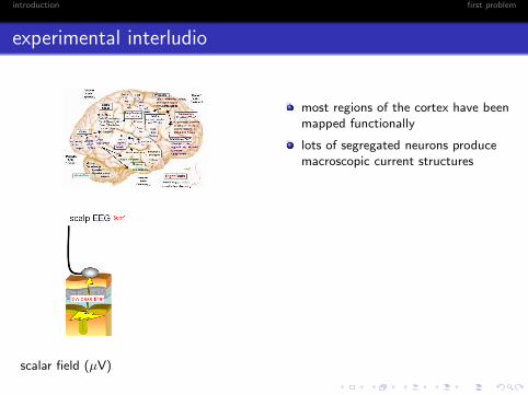
experimental interludio
most regions of the cortex have beenmapped functionally
lots of segregated neurons producemacroscopic current structures
scalar field (µV)
vector field (fT) scalar field (µV)
introduction first problem
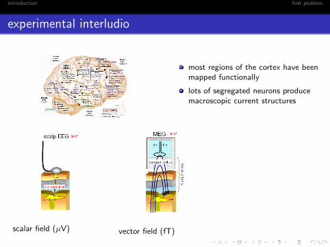
experimental interludio
most regions of the cortex have beenmapped functionally
lots of segregated neurons producemacroscopic current structures
scalar field (µV) vector field (fT)
scalar field (µV)
introduction first problem
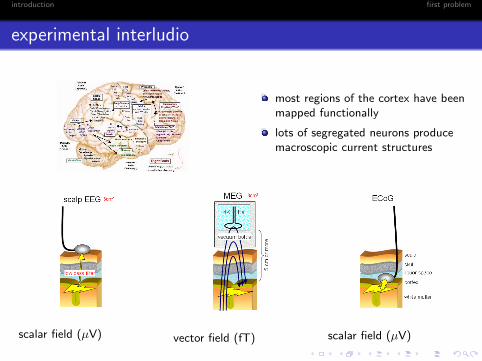
experimental interludio
most regions of the cortex have beenmapped functionally
lots of segregated neurons producemacroscopic current structures
scalar field (µV) vector field (fT) scalar field (µV)

introduction first problem
the MEG problem
b(r , t) =µ0
4π
∫Ω
[jp(r ′, t)− σ(r ′)∇v(r ′, t)]× r − r ′
|r − r ′|3 dr′
forward perspective (well-posed): given σ(r) and jp(r , t), solve ∇ · jp = ∇ · (σ∇v)and simulate b(r , t) from the biot-savart equation
inverse perspective (ill-posed): given σ(r), eliminate the secondary current effectby numerically solving ∇ · jp = ∇ · (σ∇v) and use measurements of b(r , t) toreconstruct jp(r ′, t) from the biot-savart equation (pursiainen, sorrentino, campi and
piana, inverse problems, 2011)
introduction first problem
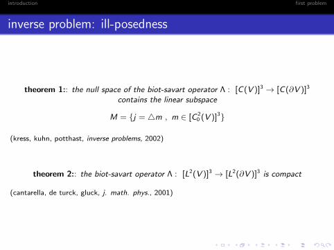
inverse problem: ill-posedness
theorem 1:: the null space of the biot-savart operator Λ : [C(V )]3 → [C(∂V )]3
contains the linear subspace
M = j = 4m , m ∈ [C 20 (V )]3
(kress, kuhn, potthast, inverse problems, 2002)
theorem 2:: the biot-savart operator Λ : [L2(V )]3 → [L2(∂V )]3 is compact
(cantarella, de turck, gluck, j. math. phys., 2001)

introduction first problem
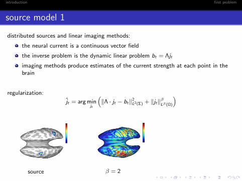
source model 1
distributed sources and linear imaging methods:
the neural current is a continuous vector field
the inverse problem is the dynamic linear problem bt = Λjt
imaging methods produce estimates of the current strength at each point in thebrain
regularization:
jt = arg minjt
(‖Λ · jt − bt‖2
L2(Σ) + ‖jt‖βLβ (Ω)
)
source β = 2 β = 1

introduction first problem
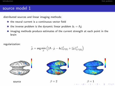
source model 1
distributed sources and linear imaging methods:
the neural current is a continuous vector field
the inverse problem is the dynamic linear problem bt = Λjt
imaging methods produce estimates of the current strength at each point in thebrain
regularization:
jt = arg minjt
(‖Λ · jt − bt‖2
L2(Σ) + ‖jt‖βLβ (Ω)
)
source
β = 2 β = 1
introduction first problem
source model 1
distributed sources and linear imaging methods:
the neural current is a continuous vector field
the inverse problem is the dynamic linear problem bt = Λjt
imaging methods produce estimates of the current strength at each point in thebrain
regularization:
jt = arg minjt
(‖Λ · jt − bt‖2
L2(Σ) + ‖jt‖βLβ (Ω)
)
source β = 2
β = 1
introduction first problem
source model 1
distributed sources and linear imaging methods:
the neural current is a continuous vector field
the inverse problem is the dynamic linear problem bt = Λjt
imaging methods produce estimates of the current strength at each point in thebrain
regularization:
jt = arg minjt
(‖Λ · jt − bt‖2
L2(Σ) + ‖jt‖βLβ (Ω)
)
source β = 2 β = 1
introduction first problem
source models 2
focal sources and non-linear parameter identification methods:
jp(r) = qδ(r − rq)
a whole active area is represented by a single current dipole
biot-savart equation in the parametric setting:
b(r , t) =µ0
4πq × r − rq|r − rq|3
− µ0
4π
∫Ω
σ(r ′)∇v(r ′, t)× r − r ′
|r − r ′|3 dr′
the parameters to estimate are q ∈ R3 and rq ∈ R3.
introduction first problem
bayesian methods
the bayes perspectives:
data and unknown are naturally modeled as random processes
regularization is effectively realized by coding prior information in probabilitydensity functions
bayes’ theorem and kolmogorov-chapman equation provide a rigorous analyticbackground (even in a non-linear setting) for tracking the dipolar source in spaceand time
particle filters allow sampling of the phase space for numerically approximating thedensity functions involved in the computation

introduction first problem
single-dipole model
first ingredient: neural currents and magnetic fields form the two stochastic processesJ1, . . . , Jt , . . . and B1, . . . ,Bt , . . . where Jt = Rt ,Qt
second ingredient: the two processes are related by
Bt = B(Jt) + Wt
Jt+1 = Jt + δJt
third ingredient: four probability density functions in the game
1 prior π(jt |b1, . . . , bt−1): prior information on the solution
2 posterior π(jt |b1, . . . , bt): solution of the inverse problem
3 likelihood π(bt |jt): forward model (the biot-savart equation) and noise model
4 transition kernel π(jt+1|jt): prior information on the dynamics

introduction first problem
bayesian tracking
(formal) solution of the dynamic MEG inverse problem
π(jt |b1:t−1) =
∫π(jt |jt−1)π(jt−1|b1:t−1)djt−1 (kolmogorov-chapman equation)
π(jt |b1:t) =π(bt |jt)π(jt |b1:t−1)
π(bt |b1:t−1)(bayes’ theorem)
jt =
∫jtπ(jt |b1:t)djt (conditional mean)
introduction first problem
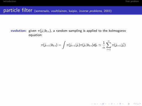
particle filter (somersalo, voultilainen, kaipio, inverse problems, 2003)
evolution: given π(jt |b1:t), a random sampling is applied to the kolmogorovequation:
π(jt+1|b1:t) =
∫π(jt+1|jt)π(jt |b1:t)djt '
1
α
α∑i=1
π(jt+1|j it )
observation: an importance sampling with importance density π(jt+1|b1:t) is appliedto approximate the posterior:
π(jt+1|b1:t+1) =α∑i=1
w it+1δ(jt+1 − j it+1) w i
t+1 ∝ π(bt+1 |j it+1)
resampling: the particles in j it+1 with large likelihood are selected
introduction first problem
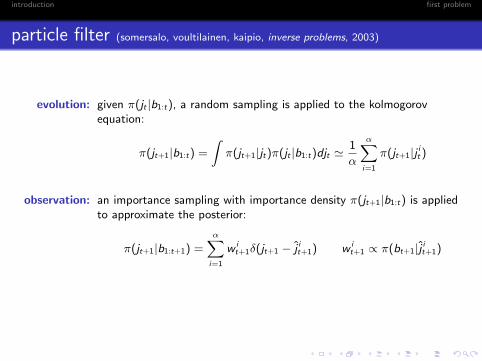
particle filter (somersalo, voultilainen, kaipio, inverse problems, 2003)
evolution: given π(jt |b1:t), a random sampling is applied to the kolmogorovequation:
π(jt+1|b1:t) =
∫π(jt+1|jt)π(jt |b1:t)djt '
1
α
α∑i=1
π(jt+1|j it )
observation: an importance sampling with importance density π(jt+1|b1:t) is appliedto approximate the posterior:
π(jt+1|b1:t+1) =α∑i=1
w it+1δ(jt+1 − j it+1) w i
t+1 ∝ π(bt+1 |j it+1)
resampling: the particles in j it+1 with large likelihood are selected
introduction first problem
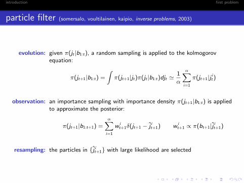
particle filter (somersalo, voultilainen, kaipio, inverse problems, 2003)
evolution: given π(jt |b1:t), a random sampling is applied to the kolmogorovequation:
π(jt+1|b1:t) =
∫π(jt+1|jt)π(jt |b1:t)djt '
1
α
α∑i=1
π(jt+1|j it )
observation: an importance sampling with importance density π(jt+1|b1:t) is appliedto approximate the posterior:
π(jt+1|b1:t+1) =α∑i=1
w it+1δ(jt+1 − j it+1) w i
t+1 ∝ π(bt+1 |j it+1)
resampling: the particles in j it+1 with large likelihood are selected
introduction first problem
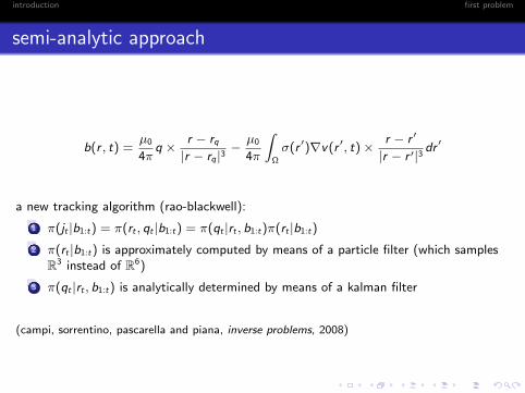
semi-analytic approach
b(r , t) =µ0
4πq × r − rq|r − rq|3
− µ0
4π
∫Ω
σ(r ′)∇v(r ′, t)× r − r ′
|r − r ′|3 dr′
a new tracking algorithm (rao-blackwell):
1 π(jt |b1:t) = π(rt , qt |b1:t) = π(qt |rt , b1:t)π(rt |b1:t)
2 π(rt |b1:t) is approximately computed by means of a particle filter (which samplesR3 instead of R6)
3 π(qt |rt , b1:t) is analytically determined by means of a kalman filter
(campi, sorrentino, pascarella and piana, inverse problems, 2008)
introduction first problem
multi-dipole model
random sets for the MEG inverse problem:
j =∑ν
i=1 qiδ(r − rqi )
parameter to optimize: ν, qi , rqi νi=1
random sets instead of random processes
belief densities instead of probability density functions
probability hypothesis density instead of conditional mean
(sorrentino, parkkonen, pascarella, campi and piana, human brain mapping, 2009)
introduction first problem
auditory stimulation
frequency: 1 KHz
MEG helmet with 306 channels (martinos center for biomedical imaging, harvarduniversity)
co-registration: T1 images (1.5 T siemens)
cortical constraints: location and orientation
introduction first problem
electrocorticography
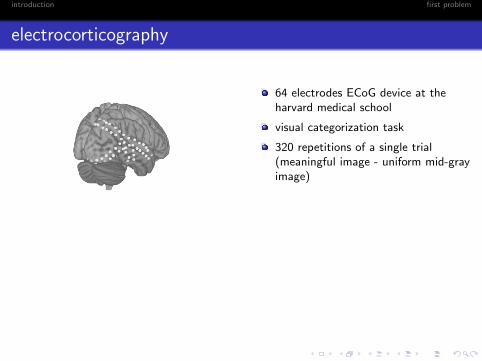
64 electrodes ECoG device at theharvard medical school
visual categorization task
320 repetitions of a single trial(meaningful image - uniform mid-grayimage)
(pascarella, todaro, clerc, serre and piana, neuroimage, in preparation)
introduction first problem
electrocorticography
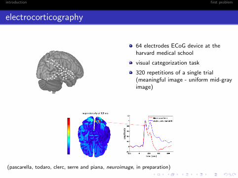
64 electrodes ECoG device at theharvard medical school
visual categorization task
320 repetitions of a single trial(meaningful image - uniform mid-grayimage)
(pascarella, todaro, clerc, serre and piana, neuroimage, in preparation)