204 Секция 2. Аналитическая экономика и прогнозирование

TWO-FACTOR PRODUCTIONS FUNCTIONS

WITH GIVEN TOTAL ELASTICITY OF PRODUCTION

Khatskevich G. A., School of Business of Belarusian State University, g. Minsk, Belarus

Pranevich F., Yanka Kupala State University of Grodno, g. Grodno, Belarus

1. Introduction. Fundamental to economic analysis is the idea of a production function. It

and its allied concept, the utility function, form the twin pillars of neoclassical economics (see [1;

2]). Roughly speaking, the production functions are the mathematical formalization of the relation-

ship between the output of a firm (industry, economy) and the inputs that have been used in obtain-

ing it. In fact, a two-factor production function is defined as a map:

: ( , ) ( , )Y K L F K L for all ( , ) ,K L G (1)

where K is the quantity of capital employed, L is the quantity of labor used, Y is the quantity of

output, and the nonnegative function F is a continuously differentiable function on the domain G

from the first quadrant 2 {( , ) : 0, 0}.R K L K L The two-factor production function (1) ex-

presses a technological relationship. It describes the maximum output obtainable, at the existing

state of technological knowledge, from given amounts of factor inputs.

At the present time, production functions apply at the level of the individual firm and the mac-

ro economy at large. At the micro level, economists use production functions to generate cost func-

tions and input demand schedules for the firm. The famous profit-maximizing conditions of optimal

factor hire derive from such microeconomics functions. At the level of the macro economy, analysts

use aggregate production functions to explain the determination of factor income shares and to

specify the relative contributions of technological progress and expansion of factor supplies to eco-

nomic growth [3–5].

Among the family of two-factor production functions (1), the most famous is the Cobb-

Douglas production function. It was introduced in 1928 by the mathematician Ch.W. Cobb and the

economist P. H. Douglas in the paper «A theory of production» [6]:

: ( , )Y K L AK L for all 2( , ) ,RK L (2)

where A is a positive constant which signifies the total factor productivity.

The Cobb-Douglas production model was generalized in 1961 by the economists K.J. Arrow,

H.B. Chenery, B.S. Minhas, and R.M. Solow [7]. They introduced the so-called Constant Elasticity

of Substitution (CES) two-factor production function (or the ACMS two-factor production function)

/: ( , ) ( )Y K L A K L for all 2( , ) ,RK L 0,A , , 0, 0, 1. (3)

Now the Cobb-Douglas production function (2) and the CES production function (3) are

widely used in economics to represent the relationship of an output to inputs. Note also that CES

production function include as special case the Cobb-Douglas production function and many other

famous production models, like a linear production model, a multinomial production function or

Leontief function. Concerning the history of development of the theory of production functions see

the papers [1; 8]. For further results concerning new production models in economic see recently

articles [9–18].

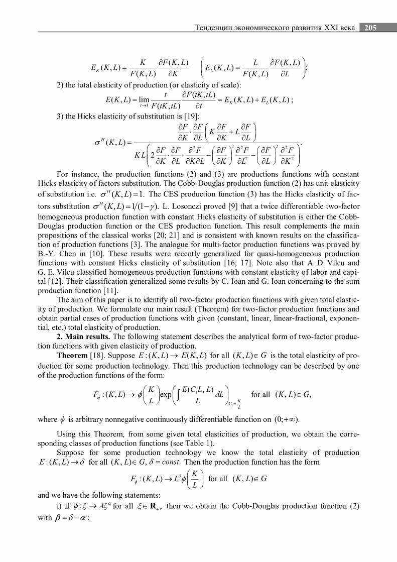
For production function (1), we recall some economic-mathematical indicators:

1) the output elasticity of capital (labor) is defined as:

205 Тенденции экономического развития XXI века

( , )( , )

( , )K

K F K LE K L

F K L K

( , )( , )

( , )L

L F K LE K L

F K L L

;

2) the total elasticity of production (or elasticity of scale):

1

( , )( , ) lim ( , ) ( , )

( , )K L

t

t F tK tLE K L E K L E K L

F tK tL t

;

3) the Hicks elasticity of substitution is [19]:

2 22 2 2

2 2

( , ) .

2

H

F F F FK L

K L K LK L

F F F F F F FKL

K L K L K L L K

For instance, the production functions (2) and (3) are productions functions with constant

Hicks elasticity of factors substitution. The Cobb-Douglas production function (2) has unit elasticity

of substitution i.e. ( , ) 1.H K L The CES production function (3) has the Hicks elasticity of fac-

tors substitution ( , ) 1 (1 ).H K L L. Losonczi proved [9] that a twice differentiable two-factor

homogeneous production function with constant Hicks elasticity of substitution is either the Cobb-

Douglas production function or the CES production function. This result complements the main

propositions of the classical works [20; 21] and is consistent with known results on the classifica-

tion of production functions [3]. The analogue for multi-factor production functions was proved by

B.-Y. Chen in [10]. These results were recently generalized for quasi-homogeneous production

functions with constant Hicks elasticity of substitution [16; 17]. Note also that A. D. Vilcu and

G. E. Vilcu classified homogeneous production functions with constant elasticity of labor and capi-

tal [12]. Their classification generalized some results by C. Ioan and G. Ioan concerning to the sum

production function [11].

The aim of this paper is to identify all two-factor production functions with given total elastic-

ity of production. We formulate our main result (Theorem) for two-factor production functions and

obtain partial cases of production functions with given (constant, linear, linear-fractional, exponen-

tial, etc.) total elasticity of production.

2. Main results. The following statement describes the analytical form of two-factor produc-

tion functions with given elasticity of production.

Theorem [18]. Suppose : ( , ) ( , )E K L E K L for all ( , )K L G is the total elasticity of pro-

duction for some production technology. Then this production technology can be described by one

of the production functions of the form:

1

1

|

( , ): ( , ) exp

KC

L

E C L LKF K L dL

L L

for all ( , ) ,K L G

where is arbitrary nonnegative continuously differentiable function on (0; ).

Using this Theorem, from some given total elasticities of production, we obtain the corre-

sponding classes of production functions (see Table 1).

Suppose for some production technology we know the total elasticity of production

: ( , )E K L for all ( , ) ,K L G .const Then the production function has the form

: ( , )K

F K L LL

for all ( , )K L G

and we have the following statements:

i) if : A for all ,R then we obtain the Cobb-Douglas production function (2)

with ;

206 Секция 2. Аналитическая экономика и прогнозирование

Table 1 – The form of production function with given total elasticity of production

No Total elasticity of production

( , , ,R f and g are continu-

ous functions)

Analytical form of production function

1. ( , )E K L ( , )K

F K L LL

2. ( , )E K L K L , expK

F K L L K LL

3. ( , )E K L f K L

|

( , ) exp

K L

fKF K L d

L

4. ( , ) ( ) ( )E K L f K g K ( ) ( )

( , ) expK f K g L

F K L dK dLL K L

5. ( , )K

E K L fL

( , ) exp ln

K KF K L L f

L L

6. ( , ) , 0K

E K L K fL

1

( , ) expK K

F K L K fL L

7. ( , ) , 0K

E K L L fL

1

( , ) expK K

F K L L fL L

8. ( , ) ( ),E K L f K L

|

1( , ) exp

K L

fKF K L d

L

Note: Developed by the authors.

ii) if /: ( )A for all ,R then we get the CES production function (3) with

;

iii) if (1 ) /: ( (1 ) )A for all ,R then we have the Lu-Fletcher pro-

duction function (Lu and Fletcher, 1968): /

(1 )

: ( , ) (1 )K

F K L A K LL

for all 2( , ) ,RK L

which for 0, 1 becomes the CES production function;

iv) if /: ((1 ) )A for all ,R then we obtain the Liu-Hildebrand pro-

duction function (Liu and Hildebrand, 1965): (1 ) /: ( , ) ((1 ) )F K L A K K L for all 2( , ) ,RK L

which for 0 becomes the CES production function;

v) if /( ): ( 2 )A a b c for all ,R then we have the Kadiyala production

function (Kadiyala, 1972): /( ): ( , ) ( 2 )F K L A aK bK L cL for all 2( , ) .RK L

where 2 1,a b c , , 0,a b c ( ) 0, ( ) 0. Since 0,b we see that the Kadiyala

function is the CES production function. If 0,c then the Kadiyala function generates directly the

Lu-Fletcher production function. For 0,a c we obtain the Cobb-Douglas production function.

Finally, for 1/ ( ) 1, 1, 1/ (1 ),a and 0,c we get the VES production function

(Revankar 1971; Sato and Hoffman, 1968):

207 Тенденции экономического развития XXI века

(1 ): ( , ) ( ( 1) )F K L AK L K for all 2( , ) .RK L

Acknowledgements. This research was supported by Belarusian State Program of Scientific

Research «Economy and humanitarian development of the Belarusian society», Project no. А65-16.

List of Sources

1. Humphrey T.M. Algebraic production functions and their uses before Cobb-Douglas. Economic Quarterly. 1997. Vol. 83/1. P. 51–83.

2. Shephard R.W. Theory of cost and production functions. Princeton, Princeton Univ. Press, 1970.

3. Kleiner G.B. Proizvodstvennye funkcii: teorija, metody, primenenie [Production functions: theory, methods, application]. Moscow, Finansy i statistika Publ., 1986.

4. Gorbunov V.K. Proizvodstvennye funkcii: teorija i postroenie [Production functions: theory and

construction]. Ulyanovsk, Ulyanovsk State University Publ., 2013.

5. Gospodarik C.G., Kovalev M.M. EAJeS-2050: global'nye trendy i evrazijskaja jekonomicheskaja politika [EAEU-2050: global trends and the Eurasian economic policies]. Minsk, BSU Publ., 2015.

6. Cobb C.W., Douglas P.H. A theory of production. American Economic Review. 1928. Vol. 18.

P. 139–165. 7. Arrow K.J., Chenery H.B., Minhas B.S., Solow R.M. Capital-labor substitution and economic effi-

ciency. The Review of Economics and Statistics. 1961. Vol. 43, No. 3. P. 225–250.

8. Mishra S.K. A brief history of production functions. IUP Journal of Managerial Economics. 2010. Vol. 8, No. 4. P. 6–34.

9. Losonczi L. Production functions having the CES property. Acta Mathematica Academiae Paeda-

gogicae Nyiregyhaziensis. 2010. Vol. 26, No. 1. P. 113–125.

10. Chen B.-Y. Classification of h-homogeneous production functions with constant elasticity of sub-stitution. Tamkang Journal of Mathematics. 2012. Vol. 43, No. 2. P. 321–328.

11. Ioan C.A., Ioan G. A generalization of a class of production functions. Applied Economics Letters.

2011. Vol. 18. P. 1777–1784. 12. Vilcu A.D., Vilcu G.E. On homogeneous production functions with proportional marginal rate of

substitution. Mathematical Problems in Engineering. 2013. Vol. 2013. P. 1–5.

16. Khatskevich G.A., Pranevich A.F. On quasi-homogeneous production functions with constant

elasticity of factors substitution. J. Belarus. State Univ. Econ. 2017. No. 1. P. 46–50. 17. Khatskevich G.A., Pranevich A.F. Quasi-homogeneous production functions with unit elasticity of

factors substitution by Hicks. J. Economy, Simulation, Forecasting. 2017. Vol. 11. P. 135–140 (in Russ.).

18. Khatskevich G.A., Pranevich A.F. Production functions with given elasticities of output and pro-duction. J. Belarus. State Univ. Econ. 2018. No. 2. P. 13–21.

19. Allen R.G. Mathematical analysis for economists. Macmillan Publ., London, 1938.

20. Uzawa H. Production functions with constant elasticities of substitution. The Review of Economic Studies. 1962. Vol. 29, No. 4. P. 291–299.

21. McFadden D. Constant elasticities of substitution production functions. Review of Economic Stud-

ies. 1963. Vol. 30. P. 73–83.

ESSENCE AND SPECIFIC FEATURES OF CLASSIFICATION

OF MONOTOWNS IN KAZAKHSTAN

Maymurunova A. A., Eurasian National University L.N. Gumilyov,

Astana, Republic of Kazakhstan

One of the reasons for the classification of cities is their functional purpose, which determines

the structure of employment, the profile of production activities of city-forming enterprises and

specialization in the structure of the social division of labor. In this sense, cities can be divided into

monofunctional (with a predominance of one functional specialization) and multifunctionalе [1].

When dividing cities into small, medium, large, large, and millionaires, the criterion of population

(city size) is used. The city-forming functions determine the functional profile of the city, its place