Embed Size (px)
Citation preview

Master Thesis
Two-dimensional Coding andDetection for data storage
on patterned media
H.W. de Jong
March 26, 2010
Graduation Committee:Dr. Ir. J.P.J. Groenland
Dr. Ir. L. AbelmannProf. Dr. Ir. C.H. Slump
Prof. Dr. M.C.ElwenspoekDr. O. Zaboronski


Abstract
An output signal from the magnetic force microscope is used for thedetection of bit values in patterned media. In a simulated signal build of a
combination of lorentzpulses the pulse distance can be changed. Thetwo-dimensional intersymbol interference will influence the ability of the
detection of the bits. Conventional detection methods are adapted for thetwo-dimensional situation and a comparison of this methods is made by
comparing bit error rates of the detectors in the presence of noise and jitter.

Contents
1 Introduction 7
2 Conventional Detection and Coding 92.1 Introduction . . . . . . . . . . . . . . . . . . . . . . . . . . . . 92.2 One-dimensional techniques . . . . . . . . . . . . . . . . . . . 9
2.2.1 Threshold Detection . . . . . . . . . . . . . . . . . . . 92.2.2 Peak detection . . . . . . . . . . . . . . . . . . . . . . 102.2.3 Partial Response Maximum Likelihood . . . . . . . . . 102.2.4 Viterbi Detection . . . . . . . . . . . . . . . . . . . . . 11
2.3 Two-dimensional techniques . . . . . . . . . . . . . . . . . . . 122.3.1 M-Algorithm . . . . . . . . . . . . . . . . . . . . . . . 122.3.2 Cross Talk Cancellation . . . . . . . . . . . . . . . . . 122.3.3 2D Viterbi Detection . . . . . . . . . . . . . . . . . . . 122.3.4 Image Processing techniques . . . . . . . . . . . . . . 12
2.4 Patterned Media Solutions . . . . . . . . . . . . . . . . . . . . 132.4.1 Iterative Decision Feedback Detection . . . . . . . . . 132.4.2 Modifying Viterbi Algorithm . . . . . . . . . . . . . . 13
2.5 Error Correction Codes . . . . . . . . . . . . . . . . . . . . . 132.5.1 Low Density Parity Check codes . . . . . . . . . . . . 142.5.2 Run Length Limited codes . . . . . . . . . . . . . . . 14
2.6 Methods in this work . . . . . . . . . . . . . . . . . . . . . . . 14
3 Detection on patterned media 173.1 Goal . . . . . . . . . . . . . . . . . . . . . . . . . . . . . . . . 173.2 Properties of the MFM signal . . . . . . . . . . . . . . . . . . 183.3 Pulse description . . . . . . . . . . . . . . . . . . . . . . . . . 19
3.3.1 One-dimensional . . . . . . . . . . . . . . . . . . . . . 193.3.2 Two-dimensional . . . . . . . . . . . . . . . . . . . . . 19
3.4 Simulation parameters . . . . . . . . . . . . . . . . . . . . . . 213.4.1 Sample rate . . . . . . . . . . . . . . . . . . . . . . . . 21
3

CONTENTS
3.4.2 Pulse period . . . . . . . . . . . . . . . . . . . . . . . 213.4.3 Pulse alignment . . . . . . . . . . . . . . . . . . . . . . 213.4.4 Non-linearities of the read-out (perspective) . . . . . . 233.4.5 Borders . . . . . . . . . . . . . . . . . . . . . . . . . . 243.4.6 Noise . . . . . . . . . . . . . . . . . . . . . . . . . . . 24
3.5 Error rate of the detection . . . . . . . . . . . . . . . . . . . . 253.6 Clocking problem . . . . . . . . . . . . . . . . . . . . . . . . . 25
4 Detector description 274.1 Threshold detector . . . . . . . . . . . . . . . . . . . . . . . . 274.2 Peak detector . . . . . . . . . . . . . . . . . . . . . . . . . . . 284.3 Triple detector . . . . . . . . . . . . . . . . . . . . . . . . . . 294.4 Decision Feedback Equalization . . . . . . . . . . . . . . . . . 324.5 Detectors on patterned media . . . . . . . . . . . . . . . . . . 35
5 Image Processing Techniques 375.1 Spot Detection . . . . . . . . . . . . . . . . . . . . . . . . . . 375.2 Feature extraction . . . . . . . . . . . . . . . . . . . . . . . . 38
5.2.1 Point spread function . . . . . . . . . . . . . . . . . . 385.2.2 Euclidean Distance . . . . . . . . . . . . . . . . . . . . 385.2.3 Convolution . . . . . . . . . . . . . . . . . . . . . . . . 405.2.4 Laplacian of the Gaussian . . . . . . . . . . . . . . . . 43
5.3 Classification . . . . . . . . . . . . . . . . . . . . . . . . . . . 445.3.1 Non-local maximum suppression . . . . . . . . . . . . 44
5.4 Image processing on patterned media . . . . . . . . . . . . . . 45
6 Results and Discussion 476.1 Patterned media simulations . . . . . . . . . . . . . . . . . . . 47
6.1.1 Jitter Influence . . . . . . . . . . . . . . . . . . . . . . 486.1.2 Medium Noise Influence . . . . . . . . . . . . . . . . . 496.1.3 Pulse distance . . . . . . . . . . . . . . . . . . . . . . 506.1.4 Lower sample rate . . . . . . . . . . . . . . . . . . . . 506.1.5 Simple coding . . . . . . . . . . . . . . . . . . . . . . . 52
6.2 Triple detector . . . . . . . . . . . . . . . . . . . . . . . . . . 52
7 Conclusions and Recommendations 577.1 Conclusions . . . . . . . . . . . . . . . . . . . . . . . . . . . . 57
7.1.1 Detector performance . . . . . . . . . . . . . . . . . . 577.1.2 Detector choice . . . . . . . . . . . . . . . . . . . . . . 577.1.3 Coding . . . . . . . . . . . . . . . . . . . . . . . . . . 587.1.4 Computation Power . . . . . . . . . . . . . . . . . . . 58
7.2 Recommendations . . . . . . . . . . . . . . . . . . . . . . . . 587.2.1 Worst-case patterns . . . . . . . . . . . . . . . . . . . 587.2.2 Computation Power . . . . . . . . . . . . . . . . . . . 59
4

CONTENTS
7.2.3 Non-linear signal patterns . . . . . . . . . . . . . . . . 597.2.4 Image Processing . . . . . . . . . . . . . . . . . . . . . 597.2.5 Bits on signal border . . . . . . . . . . . . . . . . . . . 597.2.6 Hexagonal Pattern . . . . . . . . . . . . . . . . . . . . 59
A Simulator and detector code 61A.1 Signal Simulation . . . . . . . . . . . . . . . . . . . . . . . . . 61
A.1.1 Pulse generator . . . . . . . . . . . . . . . . . . . . . . 61A.1.2 Pattern generator . . . . . . . . . . . . . . . . . . . . . 62
A.2 Detectors . . . . . . . . . . . . . . . . . . . . . . . . . . . . . 63A.2.1 Threshold detector . . . . . . . . . . . . . . . . . . . . 63A.2.2 Peak detector . . . . . . . . . . . . . . . . . . . . . . . 64A.2.3 DFE detector . . . . . . . . . . . . . . . . . . . . . . . 66A.2.4 Triple detector . . . . . . . . . . . . . . . . . . . . . . 67
A.3 Image processing . . . . . . . . . . . . . . . . . . . . . . . . . 69A.3.1 Convolution . . . . . . . . . . . . . . . . . . . . . . . . 69A.3.2 Non Local Maximum Detection . . . . . . . . . . . . . 70
Bibliography 71
5

CONTENTS
6

Chapter 1Introduction
In the current information era the demand for more and more storage capacityis constantly growing. The capacity of harddrives is still increasing, but willreach a physical limit. Magnetic pulses are written close to each other andwill soon reach a limit where they can’t be distinguished.
In the regular storage media the information storage is performed in onedimension. Tracks on a harddrive are written without awareness of surround-ing tracks. Only intersymbol interference is taken into account and intertrackinterference is being neglected.
Within the group of TST-SMI exploratory bit patterned storage media areunder research in order to have a two-dimensional read and write method. Inthis two-dimensional storage medium the bits are written in square patternson a magnetic surface. The magnetic field of each bit written on the medium isinfluenced by the fields of the surrounding bits. Two dimensional intersymbolinterference is present in these fields.
By using the knowledge of the influence of fields onto each other a detectionmechanism can be designed. An optimum should exist where a bit densityas high as possible could be reached on an acceptable error rate in detection.In this work a bit patterned medium is simulated. Detectors derived fromone-dimensional detection mechanisms have been applied as well as imageprocessing techniques for object recognition. In the simulations the bit errorrate is measured by varying medium noise and jitter.
7

Chapter 1. Introduction
8

Chapter 2Conventional Detection andCoding
2.1 Introduction
In conventional storage media a one dimensional signal is used in detection.Different detection techniques can be used for detecting bit values in a signalwith influence from medium noise and jitter. A general overview of differenttechniques is given in this chapter.
In the storage on 2D patterned media, these techniques might be useful inthe further research for optimal detection and coding.
2.2 One-dimensional techniques
2.2.1 Threshold Detection
In many detection algorithms the decisions are based on a threshold. Forexample, having a signal with two possible values: a 0 and a 1, the thresholdcan be placed at 0.5. All signal values above 0.5 are determined as a 1, allsignals below as a 0.
This way of detection is very easy to implement, but errors can easily occurwhile reading from the media. Different noise sources will influence the signaland also influence the decision.
9
Chapter 2. Conventional Detection and Coding
2.2.2 Peak detection
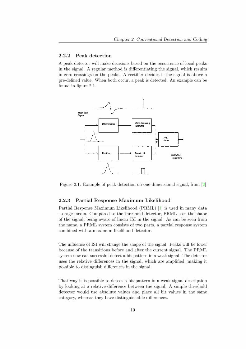
A peak detector will make decisions based on the occurrence of local peaksin the signal. A regular method is differentiating the signal, which resultsin zero crossings on the peaks. A rectifier decides if the signal is above apre-defined value. When both occur, a peak is detected. An example can befound in figure 2.1.
346 CHAPTER 11 Peak Detection Channel
Readback
Signal
). Differentiator
Rectifier p -
Zero-Crossing
Detector
, ,
I Threshold
Detector
FIGURE 11.1. Block diagram of peak detection channel.
AND
Gate
Detected
Transitions
caused by noises will be mistaken as magnetic transitions. Only when
both a zero-crossing and a rectified pulse are detected simultaneously, a
magnetic transition is found reliably.
To distinguish between adjacent transitions and to combat instabilities
of the disk rotational speed, each pulse of voltage is detected inside an
appropriate detection window, also called a timing window and should be
equal to the channel bit period. A special phase-locked loop (PLL) system
is used to provide a detection window for each channel bit. The PLL
updates its frequency based on detected pulses. Each incoming transition
or voltage pulse is searched inside its detection window. As shown in
Fig. 11.2, each pulse should be detected after the previous channel bit and
before the next channel bit, so the timing window is equal to a channel
bit period or bit cell. If a peak detection channel uses (1,7) modulation
encoding, the detection window is equal to 50% of the minimum timing
distance between two transitions that are written in the magnetic medium.
The performance of a detection channel is often characterized by
channel bit rate as well as bit error rate (BER). Bit error rate Pe is the
probability of mistaking a "0" as a "1", or mistaking a "1" as a "0" due
to the noises, distortions, or interferences in the channel. The reciprocal
of Pe means 1 error per 1/Pe bits transferred in the channel. Obviously,
Figure 2.1: Example of peak detection on one-dimensional signal, from [2]
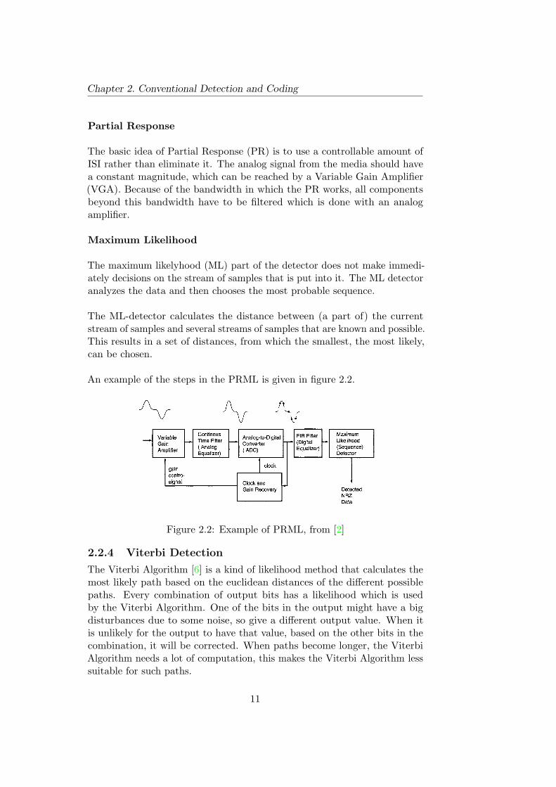
2.2.3 Partial Response Maximum Likelihood
Partial Response Maximum Likelihood (PRML) [1] is used in many datastorage media. Compared to the threshold detector, PRML uses the shapeof the signal, being aware of linear ISI in the signal. As can be seen fromthe name, a PRML system consists of two parts, a partial response systemcombined with a maximum likelihood detector.
The influence of ISI will change the shape of the signal. Peaks will be lowerbecause of the transitions before and after the current signal. The PRMLsystem now can successful detect a bit pattern in a weak signal. The detectoruses the relative differences in the signal, which are amplified, making itpossible to distinguish differences in the signal.
That way it is possible to detect a bit pattern in a weak signal descriptionby looking at a relative difference between the signal. A simple thresholddetector would use absolute values and place all bit values in the samecategory, whereas they have distinguishable differences.
10
Chapter 2. Conventional Detection and Coding
Partial Response
The basic idea of Partial Response (PR) is to use a controllable amount ofISI rather than eliminate it. The analog signal from the media should havea constant magnitude, which can be reached by a Variable Gain Amplifier(VGA). Because of the bandwidth in which the PR works, all componentsbeyond this bandwidth have to be filtered which is done with an analogamplifier.
Maximum Likelihood
The maximum likelyhood (ML) part of the detector does not make immedi-ately decisions on the stream of samples that is put into it. The ML detectoranalyzes the data and then chooses the most probable sequence.
The ML-detector calculates the distance between (a part of) the currentstream of samples and several streams of samples that are known and possible.This results in a set of distances, from which the smallest, the most likely,can be chosen.
An example of the steps in the PRML is given in figure 2.2.
362 CHAPTER 12 PRML Channels
determined. A block diagram of a typical PRML channel is shown in Fig.
12.1. 7 It consists of a variable-gain amplifier (VGA), an analog equalizer,
an analog-to-digital converter (ADC), a digital equalizer, an ML detector,
and a clock/gain recovery circuit. The circuit blocks (except the ML detec-
tor) transform the readback signal into the partial response signal as
required.
The analog readback signal from the magnetic head should have a
certain and constant level of amplification. Any variation in isolated read-
back peaks is compensated with the VGA, which gets a control signal
from the clock and gain recovery loop.
A PR channel operates within a certain bandwidth, meaning that the
spectral components beyond the bandwidth have to be cut off. This is done
with the continuous time filter or analog equalizer. The other function
sometimes performed by the analog equalizer is to modify the frequency
response of the channel. The modification of the frequency response is
sometimes required to adjust the shape of the readback signal from the
head. For example, it may be necessary to adjust the pulse width to make
it proportional to the distance between transitions. The analog equalizer
is implemented as a linear filter with a programmable frequency response
including a variable cutoff frequency and boost. The analog signal at
the equalizer output generally has a slightly different shape than the
unmodified signal directly from the head.
The signal from the analog equalizer is sampled (or digitized) with
the ADC. The sampling is initiated by a clock signal at the rate of exactly
one sample per channel bit period. The frequency and phase of the clock
.• Variable ~_~ Continous Gain Time Filter Amplifier ( Analog Equalizer)
gain control signal
~.~ Analog-to-Digital ~ Converter (ADC)
I clock I
Cl~ ry ~'J
FIGURE 12.1. Block diagram of typical PRML channel.
Maximum Likelihood (Sequence) Detector
Detected NRZ Data
Figure 2.2: Example of PRML, from [2]
2.2.4 Viterbi Detection
The Viterbi Algorithm [6] is a kind of likelihood method that calculates themost likely path based on the euclidean distances of the different possiblepaths. Every combination of output bits has a likelihood which is usedby the Viterbi Algorithm. One of the bits in the output might have a bigdisturbances due to some noise, so give a different output value. When itis unlikely for the output to have that value, based on the other bits in thecombination, it will be corrected. When paths become longer, the ViterbiAlgorithm needs a lot of computation, this makes the Viterbi Algorithm lesssuitable for such paths.
11
Chapter 2. Conventional Detection and Coding
2.3 Two-dimensional techniques
2.3.1 M-Algorithm
The paper from Zadeh [3] describes a solution for a multitrack magneticrecording medium. In this description the input data is given as a two dimen-sional signal. In the channel model it is assumed there is only interferencefrom adjacent tracks.
The several standard methods as Partial Response and Viterbi detectors aredescribed, however, the problem with such detectors is the high number ofstates for only a small number tracks to be considered at one readout. TheM-Algorithm is a detector with a reduced complexity. From all paths the Mbest paths are stored. An advantage of the M -algorithm over the ViterbiAlgorithm is the reduced number of paths, which makes it more suitable forlonger paths and decreases the computations.
In Tosi [4] also a description for a system using the M -algorithm is given.This paper describes a partial response detection for a multi-track system.
2.3.2 Cross Talk Cancellation
In the thesis of Immink [5] the Cross Talk Cancellation (XTC) is discussed.With this technique three tracks are read out simultaneously and filteredversions of the two outer tracks are subtracted from the middle track inorder to cancel the influence from the two outer tracks on the middle track.A quite simple method for improving the detection.
2.3.3 2D Viterbi Detection
The paper of Kato [7] to which is referred in Immink [5] has some interestingpoints about 2D Viterbi detection, but these are just seperated Viterbi detec-tors. The 2D viterbi detection described in Immink made some improvementson the Multitrack Viterbi Algorithm it is referring to. These refinementsinclude taking into account weighing of contributions and taking into accountother contributions.
Also non-linear ISI can be handled, by using the output of a previouscalculated value of a state. The complexity of the algorithm has also beendecreased.
2.3.4 Image Processing techniques
By plotting the output signal of a patterned medium as an image, this readoutsignals look like images with bright and dark dots on a gray background.With image processing techniques the dots in these signals can be detected.
12
Chapter 2. Conventional Detection and Coding
In chapter 5 more about these methods is given.
2.4 Patterned Media Solutions
Several papers are published about the two-dimensional detection in pat-terned media storage (PMS). An overview is given below.
2.4.1 Iterative Decision Feedback Detection
In Keskinoz [8] a description for a 2D detector for a patterned media isworked out in detail. The paper has 2 parts, one for a Iterative DecisionFeedback Detection (IDFD) system and a 2D Generalized Partial Response(2D-GPR) with 1D Viterbi.
These techniques require more computations and have some requirements.IDFD requires all readings to be available to detect the information symbols.The 2D-GPR method performs better than IDFD under the same compu-tational load, whereas IDFD could achieve a higher SNR, employing moreiterations.
2.4.2 Modifying Viterbi Algorithm
Nabavi [9] describes a modified version of the Viterbi Algorithm for bit-patterned media. This algorithm improves the BER while the complexity isnot significantly increased. There are the same number of states, but thenumber of branches between these states increases.
The track misregistration (TMR) or read head offset is also taken intoaccount, where as expected the modified Viterbi is more tolerant than thenormal Viterbi.
2.5 Error Correction Codes
Errors will always occur in writing and reading data, due to noise andinterference. To be able to correct errors, the user data is encoded with errorcorrection codes (ECC).
Errors can occur in two types: single-bit errors and bursts of errors. Asingle-bit error can occur through a short noise event, which results in anextra pulse or a missing pulse. Bursts of errors usually occur through defectsof the medium.
The use of ECC improves the reliability of data recovery. There are differentECC designed to correct a finite number of corrupted bits. Of course encodingrequires more bits for the information to be stored on the disc, but the storage
13

Chapter 2. Conventional Detection and Coding
capacity of a medium can be improved with the ECC.
2.5.1 Low Density Parity Check codes
To improve the performance of the system, it is important to use a codewhich is optimized for the channel properties. Combinations of bits whichare hard to detect have to be avoided in order to keep the error rate as lowas possible.
The use of the right codes already inserts some redundancy in the bits storedon the media. In [10] several methods for the application of Low-DensityParity-Check (LDPC) codes are given, as well as the construction of optimalcodes for different channel models.
A consequence on the use of complex coding is the complexity of the decodingthat has to be done after the detection of the signal.
2.5.2 Run Length Limited codes
Run Length Limited (RLL) codes are codes which have a minimum and amaximum number of a value used after each other. For magnetic storagethese values are a transition or no transition, a 1 or a 0. RLL Codes aretypically referenced as (m/n)(d,k) codes. (m/n) Means: m user bits aremapped on n encoded bits, where n ≥ m. d is the minimum allowed numberof consecutive ”0”s between two ”1”s (d ≥ 0). And k is the maximum numberof consecutive ”0”s between two ”1”s (k ≥ 0).
In the paper from Kato [7] a multi-track recording system with the use of2D-PRML and 2D-RLL is described.
2.6 Methods in this work
While the storage medium in this work is in a exploratory status, the detectionis started with a threshold detection on the two dimensional signal. Also two-dimensional versions of the peak detector and a decision feedback detectorare applied.A method using 3x3 samples per bit, which is designed within the TST-SMIgroup is implemented and some image processing techniques are applied onthe signal and a comparison with the regular methods is made.
The results of the detectors are measured by the error rate of the detected bits.By varying the medium noise and the jitter on the medium, a comparisonbetween the methods is made.
In the first comparison between the detectors no specific coding methods on
14

Chapter 2. Conventional Detection and Coding
the input bits are applied. Only a simple coding method designed in theTST-SMI group is used for comparison with an uncoded situation. In thiscoding the worst-case patterns with bits of the same value are preventedfrom being present in the input signal. In every 3x3 bitpattern always onebit has value 1 and one bit is a 0.
The current implementation of this coding decreases the bit density by about20 percent, by filling the 3x3 bitpatterns with a 1 and 0 without taking theother bit values into account. A more advanced implementation could reducethis density decrease.
15

Chapter 2. Conventional Detection and Coding
16
Chapter 3Detection on patterned media
Because of the exploratory status of this storage medium candidate, manydesign decisions have not been made yet. The readout of the signal mightbe influenced by changes in parts of the system. In order to perform thesimulations, assumptions have been made which are described in this chapter.
3.1 Goal
The goal of this master assignment is to compare detection mechanisms onthe aspects of medium noise and jitter. On the storage medium the bits arestored in a two-dimensional bit pattern. On conventional storage media thebits have only influence from the previous and next bit on the same track, theintersymbol interference (ISI). In a two-dimensional medium the bit patternswould have influence from the surrounding bits in two dimensions, so called2D-ISI. Which is in fact an equivalent to Intertrack Interference (ITI) inconventional media.
Other important aspects in comparing detectors is the clocking problem.A clock-less detector, where bits are detected autonomously would be verypractical. To be concurring with conventional storage media the informationshould be detected on a high speed, with a sample rate as low as possibleand a high bit-density on the medium.
In the two-dimensional storage and detection field more research has alsobeen done for example by Wood et. al. in [14]. In that paper the feasibilityof a magnetic recording at 10 terabits per square inch is investigated. Aconventional medium is used, but more advanced write and read methods
17
Chapter 3. Detection on patterned media
are necessary in order to reach a higher bit density. Every bit is stored ononly 2 grains on the medium. The information across different tracks is usedin the signal processing. The paper concludes that a fine grained mediumis necessary in order to be able to reach the high density for 10 terabitsper square inch and a practical two-dimensional detection scheme should bedeveloped for detection of the bits with accurate timing and positioning.
In the next chapters various types of detection are described, includingthe conventional one-dimensional methods. Also techniques from the imageprocessing field are taken into account, the signal can be seen as a picture withblack and white dots on it. This can be described as an object recognitionproblem in image processing.
3.2 Properties of the MFM signal
The simulated signal is based on the experimental recording setup with amagnetic force microscope (MFM) from the TST-SMI group. It is in detaildescribed in [12] and [13]. A CoNi/Pt multilayer is used as the recordingmedium and the periodicity of pulses goes down to 150 nm. The field isscanned over the x and y direction. Writing the information is achievedby approaching a MFM-tip to the medium in the presence of an externalmagnetic field in the z direction. The read signal is a result from the vibratingMFM tip in the stray field of the magnetized dots. The signal is proportionalto the second z derivative VMFM (x) ≈ (d2Hz(x)/dz2) integrated over thetip volume.
The MFM signal can be simulated by a superposition of the individual MFMresponses. When the individual pulses are written close to each other, theresponses of these pulses overlap, influencing the output signal. This is the(two-dimensional) intersymbol interference which influences detection.
An example of a typical MFM output signal can be found in figure 3.1. Itshould be mentioned that while this image looks like a surface with dots onit, this is not how the recording medium surface looks like, but a result fromthe vibrating tip.
The magnetostatic details are not described further here. In the simulationsthe signal is build from overlapping pulses, which characteristics are describedfurther.
18
Chapter 3. Detection on patterned media
Figure 3.1: Output signal from MFM
3.3 Pulse description
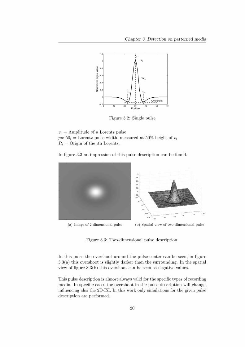
3.3.1 One-dimensional
Rather than taking the full magnetostatic details into account, we can in firstinstance approximate the signal by a superposition of Lorentzpulses. Thisconsiderably speeds up calculation time. The Lorentz function is defined asy = 1
1+x2 . ISI is introduced by an overshoot of the pulse, also described by aLorentzpulse. The resulting pulse description for one bit is a combination ofthree Lorentzpulses:
pulse(x) =3∑
i=1
vi
1 + ( x−xipw 50i/2)
(3.1)
Wherevi = Amplitude of a Lorentz pulsepw 50i = Lorentz pulse width, measured at 50% height of vi
xi = Origin of the ith Lorentz.
A single pulse used in the simulations can be seen in figure 3.2.
3.3.2 Two-dimensional
The two-dimensional situation is just an expansion of the one-dimensionalpulse from equation 3.1. The pulse is now described in two dimensions:
R =√X2 + Y 2
pulse(R) =3∑
i=1
vi
1 + ( R−Ripw 50i/2)
(3.2)
19
Chapter 3. Detection on patterned media
! "! #! $! %! &! '!!!(#
!
!(#
!(%
!('
!()
"
"(#
*+,-.-+/
0+1234-5678,-9/348:34;6
<#
<"
<$
=:61,>++.
*?&!
:#
Figure 3.2: Single pulse
vi = Amplitude of a Lorentz pulsepw 50i = Lorentz pulse width, measured at 50% height of vi
Ri = Origin of the ith Lorentz.
In figure 3.3 an impression of this pulse description can be found.
5 10 15 20 25 30 35 40
5
10
15
20
25
30
35
40
(a) Image of 2 dimensional pulse
−30 −20 −10 0 10 20
−30
−20
−10
0
10
20−0.2
0
0.2
0.4
0.6
0.8
1
(b) Spatial view of two-dimensional pulse
Figure 3.3: Two-dimensional pulse description.
In this pulse the overshoot around the pulse center can be seen, in figure3.3(a) this overshoot is slightly darker than the surrounding. In the spatialview of figure 3.3(b) this overshoot can be seen as negative values.
This pulse description is almost always valid for the specific types of recordingmedia. In specific cases the overshoot in the pulse description will change,influencing also the 2D-ISI. In this work only simulations for the given pulsedescription are performed.
20
Chapter 3. Detection on patterned media
3.4 Simulation parameters
3.4.1 Sample rate
The signal which will be used in the detectors is a sampled version of theMFM respons of the magnetic field. With a high sample rate there is a betterdescription of the pulses on the medium, more samples are available per bit.
In simulations the sample rate is varied. From earlier work within the TST-SMI Group a sample rate of 3x3 samples per bit has been used in detection.The threshold detector uses only one sample per bit and for the remainingdetectors also higher sample rates have been used for comparison of thedetector performance on varying sample rates.
With higher sample rates more computation power is needed for the detection.Whether or not this is acceptable depends on the achieved gain in error rate.
3.4.2 Pulse period
The bits written on the medium are placed at some distance from eachother, the pulse period. The description of the pulse is given in section 3.3.While varying the pulse period, also the influence from one pulse on theneighbouring pulses will vary. Specific patterns can have such an influenceon surrounding pulses that bit values are hard to detect.
A small pulse period will result in a high bit density on the medium, whilemore errors will occur in detection. With a slightly larger distance betweenpulses the 2D-ISI will change. The error rate can be reduced and compensatefor the loss in bit density. An optimum therefore will exist.
In figure 3.4 examples of pulse distances can be seen for a one dimensionalsignal. For a two-dimensional signal the same principle holds for bothdimensions. These figures show a signal with two pulses of the same value.In case of two opposite values, the pulses will also influence, but increase thebit value of the neighbouring value, as is given in figure 3.5.
3.4.3 Pulse alignment
The written pulses can be organized in different patterns. Two main pat-terns can be distinguished: a square pattern and a hexagonal pattern. Animportant difference between the square and hexagonal ordering is the equaldistance between all direct neighbouring pulses in the hexagonal signal, sothat these influences are also equal. In the square pattern the pulses willhave different influences on each other. At this moment only the square typeof ordering is used in the MFM and in this work only the square pattern isused in the detector.
21
Chapter 3. Detection on patterned media
0 10 20 30 40 50 60 70 80−0.2
0
0.2
0.4
0.6
0.8
1
1.2
Position
Nor
mal
ized
sig
nal v
alue
Period
(a) Big distance betweenpulses
0 10 20 30 40 50 60 70−0.2
0
0.2
0.4
0.6
0.8
1
1.2
Position
Nor
mal
ized
sig
nal v
alue
Period
(b) Small distance betweenpulses
! "! #! $! %! &! '! (!!!)#
!
!)#
!)%
!)'
!)*
"
")#
+,-./.,0
1,2345.6789-.:0459;45<7
(c) Combined signal of twopulses of fig 3.4(b)
Figure 3.4: Example of different pulse distances.
0 10 20 30 40 50 60 70−1.5
−1
−0.5
0
0.5
1
1.5
Position
Nor
mal
ized
sig
nal v
alue
(a) Two opposite bit values
0 10 20 30 40 50 60 70−1.5
−1
−0.5
0
0.5
1
1.5
Position
Nor
mal
ized
sig
nal v
alue
(b) Combined signal of bit val-ues
Figure 3.5: Pulses with opposite values.
22
Chapter 3. Detection on patterned media
In figure 3.6 examples of the square and hexagonal pulse alignment can befound. With the use of a hexagonal alignment the distance between the rowsis smaller, to keep the distance to the pulses in the neighbouring rows thesame as the pulses on the same row.
20 40 60 80 100 120 140 160 180 200
20
40
60
80
100
120
140
160
180
200 (a) Square pulse alignment0 20 40 60 80 100 120 140 160 180 200
0
20
40
60
80
100
120
140
160
180
200 (b) Hexagonal pulse alignment
Figure 3.6: Square and hexagonal pulse alignment
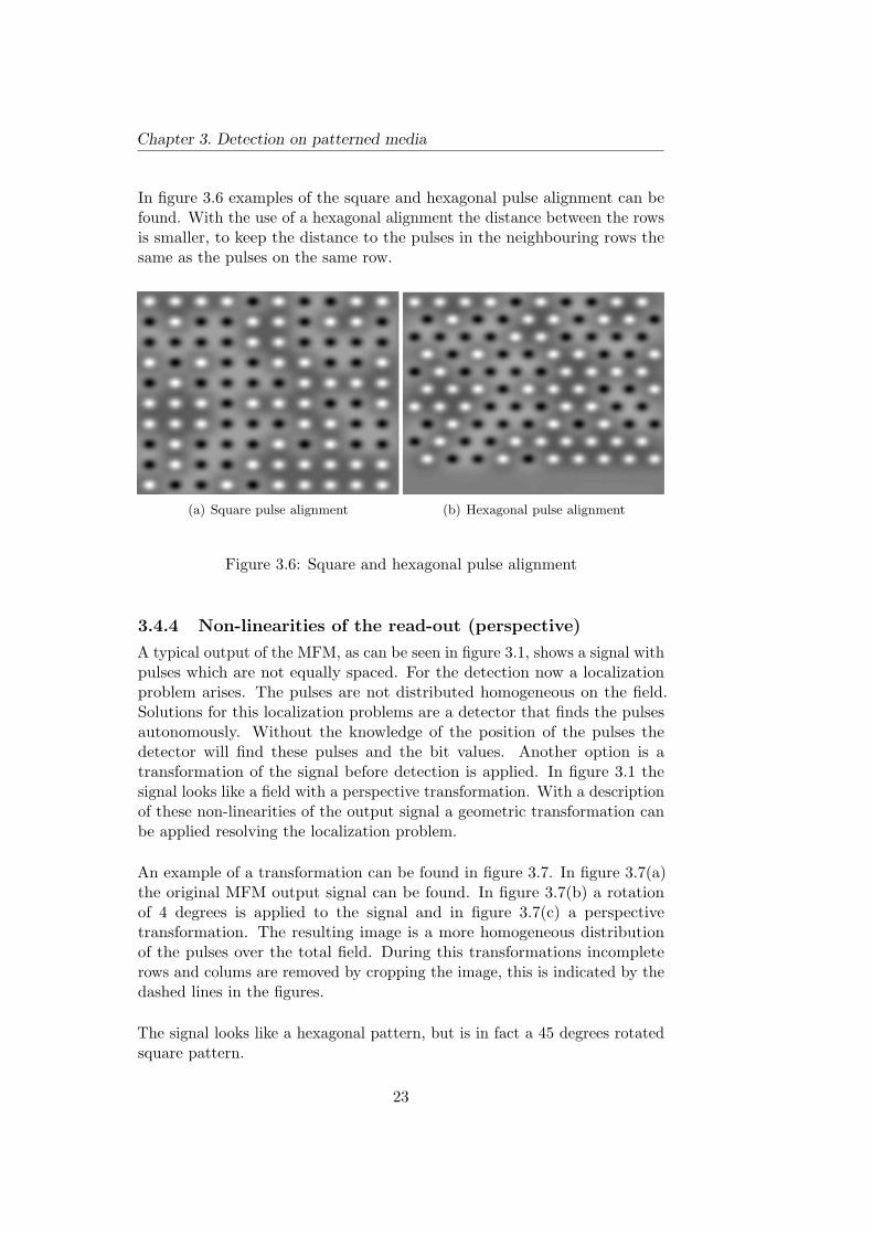
3.4.4 Non-linearities of the read-out (perspective)
A typical output of the MFM, as can be seen in figure 3.1, shows a signal withpulses which are not equally spaced. For the detection now a localizationproblem arises. The pulses are not distributed homogeneous on the field.Solutions for this localization problems are a detector that finds the pulsesautonomously. Without the knowledge of the position of the pulses thedetector will find these pulses and the bit values. Another option is atransformation of the signal before detection is applied. In figure 3.1 thesignal looks like a field with a perspective transformation. With a descriptionof these non-linearities of the output signal a geometric transformation canbe applied resolving the localization problem.
An example of a transformation can be found in figure 3.7. In figure 3.7(a)the original MFM output signal can be found. In figure 3.7(b) a rotationof 4 degrees is applied to the signal and in figure 3.7(c) a perspectivetransformation. The resulting image is a more homogeneous distributionof the pulses over the total field. During this transformations incompleterows and colums are removed by cropping the image, this is indicated by thedashed lines in the figures.
The signal looks like a hexagonal pattern, but is in fact a 45 degrees rotatedsquare pattern.
23
Chapter 3. Detection on patterned media
Originele afbeelding
200 400 600 800 1000 1200
100
200
300
400
500
600
700
800
900
1000
1100
(a) MFM output signal
Rotated Image
100 200 300 400 500 600 700 800 900 1000 1100
100
200
300
400
500
600
700
800
900
1000
(b) MFM output after rota-tion
Transformed Image
100 200 300 400 500 600 700 800 900 1000
100
200
300
400
500
600
700
800
900
1000
(c) MFM output after per-spective transformation
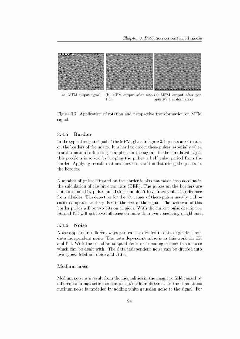
Figure 3.7: Application of rotation and perspective transformation on MFMsignal.
3.4.5 Borders
In the typical output signal of the MFM, given in figure 3.1, pulses are situatedon the borders of the image. It is hard to detect these pulses, especially whentransformation or filtering is applied on the signal. In the simulated signalthis problem is solved by keeping the pulses a half pulse period from theborder. Applying transformations does not result in disturbing the pulses onthe borders.
A number of pulses situated on the border is also not taken into account inthe calculation of the bit error rate (BER). The pulses on the borders arenot surrounded by pulses on all sides and don’t have intersymbol interferencefrom all sides. The detection for the bit values of these pulses usually will beeasier compared to the pulses in the rest of the signal. The overhead of thisborder pulses will be two bits on all sides. With the current pulse descriptionISI and ITI will not have influence on more than two concurring neighbours.
3.4.6 Noise
Noise appears in different ways and can be divided in data dependent anddata independent noise. The data dependent noise is in this work the ISIand ITI. With the use of an adapted detector or coding scheme this is noisewhich can be dealt with. The data independent noise can be divided intotwo types: Medium noise and Jitter.
Medium noise
Medium noise is a result from the inequalities in the magnetic field caused bydifferences in magnetic moment or tip/medium distance. In the simulationsmedium noise is modelled by adding white gaussian noise to the signal. For
24
Chapter 3. Detection on patterned media
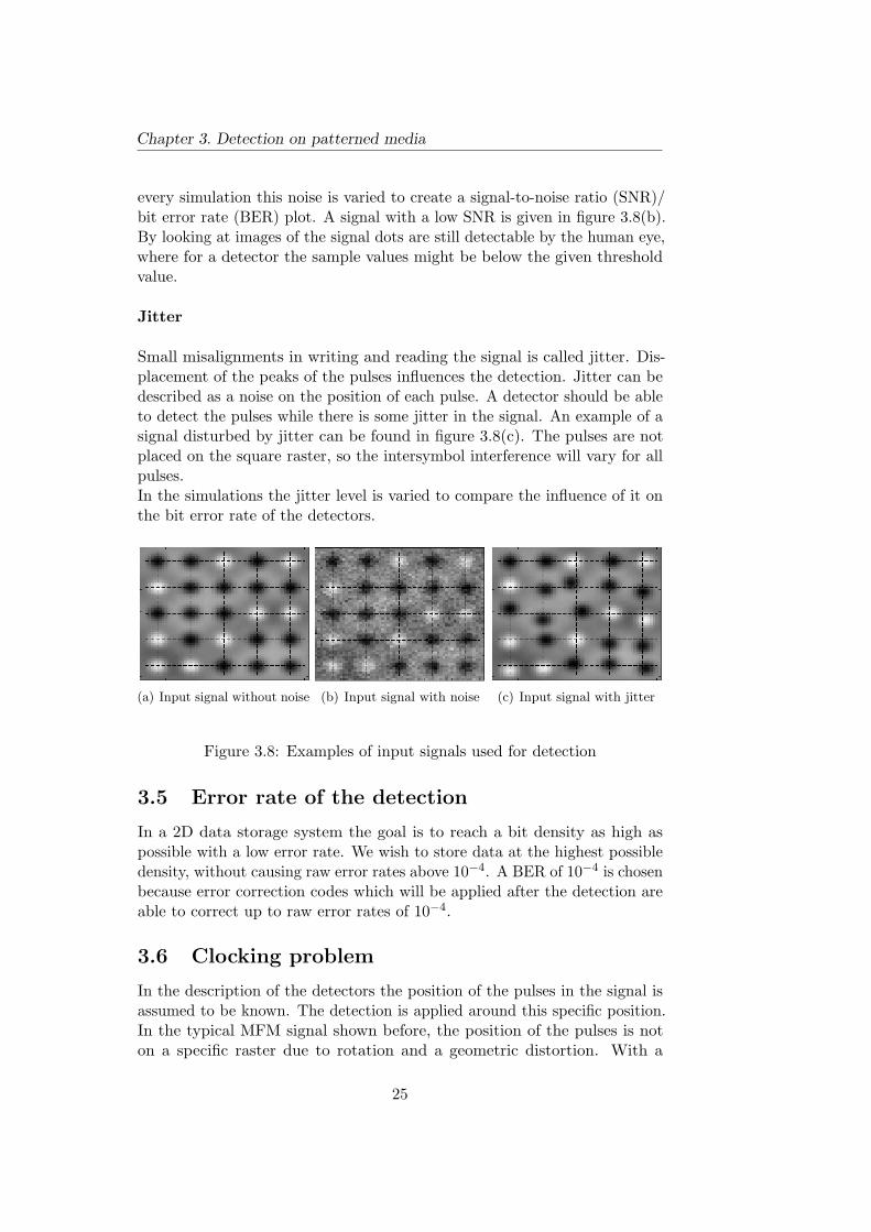
every simulation this noise is varied to create a signal-to-noise ratio (SNR)/bit error rate (BER) plot. A signal with a low SNR is given in figure 3.8(b).By looking at images of the signal dots are still detectable by the human eye,where for a detector the sample values might be below the given thresholdvalue.
Jitter
Small misalignments in writing and reading the signal is called jitter. Dis-placement of the peaks of the pulses influences the detection. Jitter can bedescribed as a noise on the position of each pulse. A detector should be ableto detect the pulses while there is some jitter in the signal. An example of asignal disturbed by jitter can be found in figure 3.8(c). The pulses are notplaced on the square raster, so the intersymbol interference will vary for allpulses.In the simulations the jitter level is varied to compare the influence of it onthe bit error rate of the detectors.
(a) Input signal without noise (b) Input signal with noise (c) Input signal with jitter
Figure 3.8: Examples of input signals used for detection
3.5 Error rate of the detection
In a 2D data storage system the goal is to reach a bit density as high aspossible with a low error rate. We wish to store data at the highest possibledensity, without causing raw error rates above 10−4. A BER of 10−4 is chosenbecause error correction codes which will be applied after the detection areable to correct up to raw error rates of 10−4.
3.6 Clocking problem
In the description of the detectors the position of the pulses in the signal isassumed to be known. The detection is applied around this specific position.In the typical MFM signal shown before, the position of the pulses is noton a specific raster due to rotation and a geometric distortion. With a
25
Chapter 3. Detection on patterned media
detector that finds the pulses itself the knowledge of this information won’tbe necessary and the problem with rotation and distortion doesn’t need tobe solved before the detection is applied.
The detectors have been implemented with some boundary conditions. Asinput to the system a signal is given with a known number of written bits.The detectors assume the bits to be distributed homogeneous, which makesit possible to divide the signal in regions for every bit.
One of the problems in this autonomous detection is the noise influence onthe signal. Extra pulses might occur or pulses become below threshold. Theinfluence of jitter is a problem when the peaks are written close to eachother, they might get written so close near each other that they won’t bedistinguishable and will appear as just one pulse. This makes detection verydifficult.
As a result from the 2D-ISI extra pulses might occur in the signal. Amechanism where a minimal distance is required between the samples of thedetected bits can reduce the number of errors resulting from this influence.
The distortions visible in the output signal of the MFM influence the lineardistribution of the pulses over the signal. The detection could compensatethis by evaluating each detected pulse and adapt the expected pulse forthe last few detected pulses. When the pulse period becomes wider thisis compensated during detection and does not lead to an error. Such anerror detection mechanism would cost extra computation power. Anotherpossibility to compensate for the non-linearities is to apply transformationtechniques. If the non-linearities of the MFM signal can be described thiscan be used for transformation.
In simulations these distortions are not taken into account. The pulses areexpected to be distributed homogeneously on the medium.
26
Chapter 4Detector description
This chapter describes the conventional detectors used for the simulationsin this work. In appendix A the code for all detectors can be found. In thedetectors the expected position of the pulses is assumed to be on a squarepattern.
4.1 Threshold detector
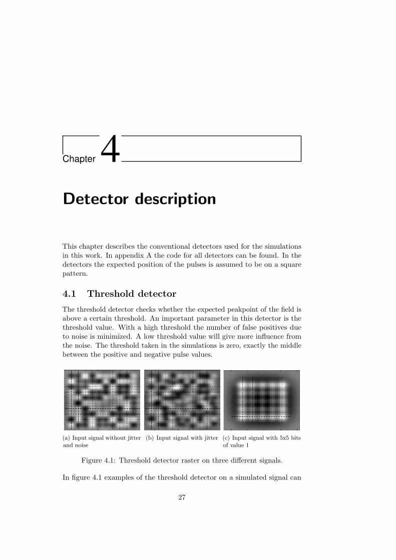
The threshold detector checks whether the expected peakpoint of the field isabove a certain threshold. An important parameter in this detector is thethreshold value. With a high threshold the number of false positives dueto noise is minimized. A low threshold value will give more influence fromthe noise. The threshold taken in the simulations is zero, exactly the middlebetween the positive and negative pulse values.
(a) Input signal without jitterand noise
(b) Input signal with jitter (c) Input signal with 5x5 bitsof value 1
Figure 4.1: Threshold detector raster on three different signals.
In figure 4.1 examples of the threshold detector on a simulated signal can
27
Chapter 4. Detector description
be found. The sample values are the crossings of the dashed raster lines.In this figure errors occur, as a result from the intersymbol and intertrackinterference.
This detector takes the value of the signal on fixed sample points, resultingin a lot of influence from jitter on it. This shift of peaks will result in lowersample values at the expected points. With high jitter, a sample value canbe below threshold and the bit value will flip. In figure 4.1(a) and 4.1(b)an input signal without and with jitter can be seen, both with the same bitpattern. In figure 4.1(b) a lot of pulses are not on the expected peak points.
In the 5x5 bitpattern in figure 4.1(c) all bits have value one and the interfer-ence has such an influence on the bits in the center, that the values on thethreshold detector will flip. The crossings of the raster lines in the figure arethe sample points of the threshold detector.
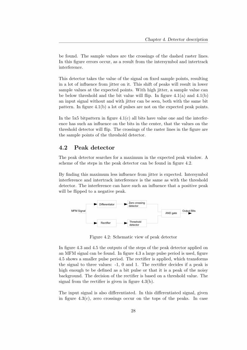
4.2 Peak detector
The peak detector searches for a maximum in the expected peak window. Ascheme of the steps in the peak detector can be found in figure 4.2.
By finding this maximum less influence from jitter is expected. Intersymbolinterference and intertrack interference is the same as with the thresholddetector. The interference can have such an influence that a positive peakwill be flipped to a negative peak.
MFM Signal Output BitsAND gate
Differentiator
Rectifier
Zero crossingdetector
Thresholddetector
Figure 4.2: Schematic view of peak detector
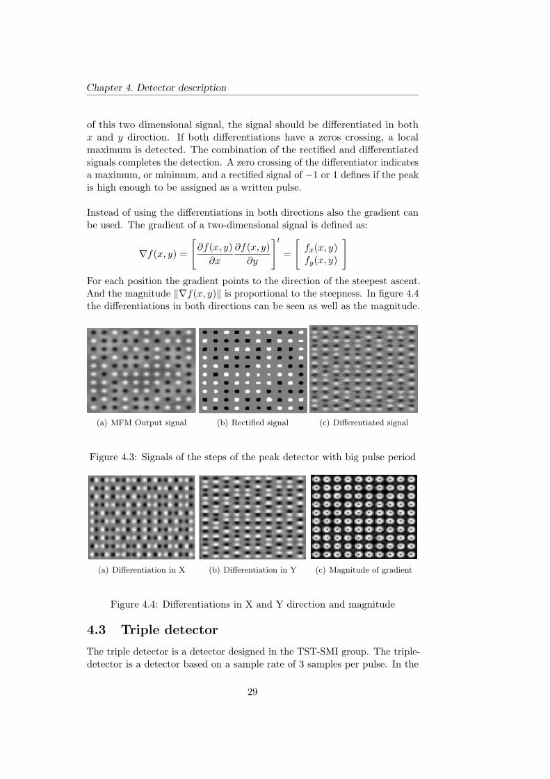
In figure 4.3 and 4.5 the outputs of the steps of the peak detector applied onan MFM signal can be found. In figure 4.3 a large pulse period is used, figure4.5 shows a smaller pulse period. The rectifier is applied, which transformsthe signal to three values: -1, 0 and 1. The rectifier decides if a peak ishigh enough te be defined as a bit pulse or that it is a peak of the noisybackground. The decision of the rectifier is based on a threshold value. Thesignal from the rectifier is given in figure 4.3(b).
The input signal is also differentiated. In this differentiated signal, givenin figure 4.3(c), zero crossings occur on the tops of the peaks. In case
28
Chapter 4. Detector description
of this two dimensional signal, the signal should be differentiated in bothx and y direction. If both differentiations have a zeros crossing, a localmaximum is detected. The combination of the rectified and differentiatedsignals completes the detection. A zero crossing of the differentiator indicatesa maximum, or minimum, and a rectified signal of −1 or 1 defines if the peakis high enough to be assigned as a written pulse.
Instead of using the differentiations in both directions also the gradient canbe used. The gradient of a two-dimensional signal is defined as:
∇f(x, y) =
[∂f(x, y)∂x
∂f(x, y)∂y
]t
=
[fx(x, y)fy(x, y)
]For each position the gradient points to the direction of the steepest ascent.And the magnitude ‖∇f(x, y)‖ is proportional to the steepness. In figure 4.4the differentiations in both directions can be seen as well as the magnitude.
mfmOutput
20 40 60 80 100 120 140
20
40
60
80
100
120
140
(a) MFM Output signal20 40 60 80 100 120 140
20
40
60
80
100
120
140
(b) Rectified signal
differentiated output
20 40 60 80 100 120 140
20
40
60
80
100
120
140
(c) Differentiated signal
Figure 4.3: Signals of the steps of the peak detector with big pulse period
(a) Differentiation in X (b) Differentiation in Y (c) Magnitude of gradient
Figure 4.4: Differentiations in X and Y direction and magnitude
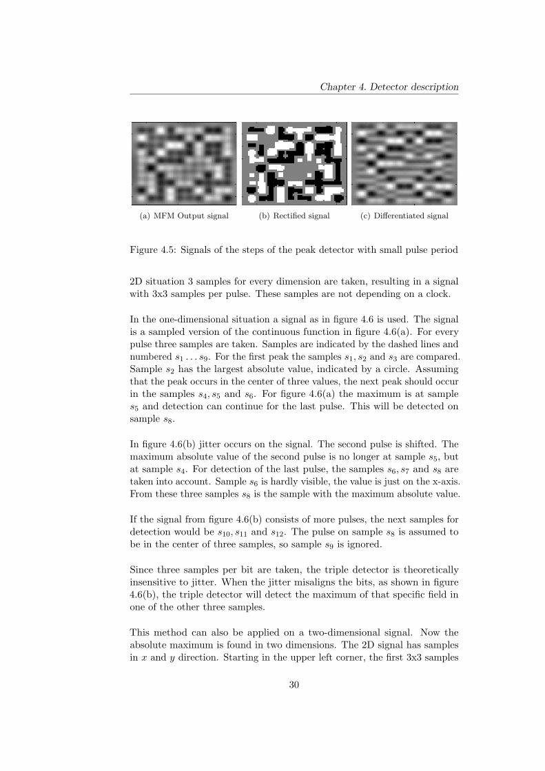
4.3 Triple detector
The triple detector is a detector designed in the TST-SMI group. The triple-detector is a detector based on a sample rate of 3 samples per pulse. In the
29
Chapter 4. Detector description
(a) MFM Output signal (b) Rectified signal (c) Differentiated signal
Figure 4.5: Signals of the steps of the peak detector with small pulse period
2D situation 3 samples for every dimension are taken, resulting in a signalwith 3x3 samples per pulse. These samples are not depending on a clock.
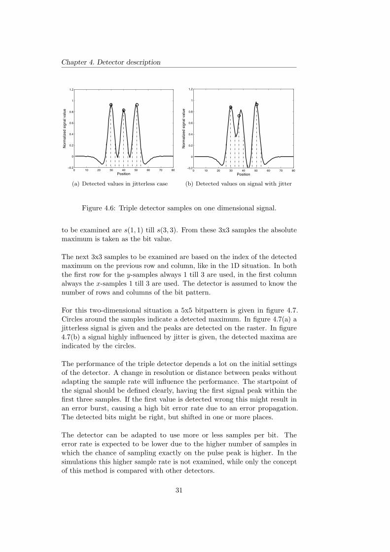
In the one-dimensional situation a signal as in figure 4.6 is used. The signalis a sampled version of the continuous function in figure 4.6(a). For everypulse three samples are taken. Samples are indicated by the dashed lines andnumbered s1 . . . s9. For the first peak the samples s1, s2 and s3 are compared.Sample s2 has the largest absolute value, indicated by a circle. Assumingthat the peak occurs in the center of three values, the next peak should occurin the samples s4, s5 and s6. For figure 4.6(a) the maximum is at samples5 and detection can continue for the last pulse. This will be detected onsample s8.
In figure 4.6(b) jitter occurs on the signal. The second pulse is shifted. Themaximum absolute value of the second pulse is no longer at sample s5, butat sample s4. For detection of the last pulse, the samples s6, s7 and s8 aretaken into account. Sample s6 is hardly visible, the value is just on the x-axis.From these three samples s8 is the sample with the maximum absolute value.
If the signal from figure 4.6(b) consists of more pulses, the next samples fordetection would be s10, s11 and s12. The pulse on sample s8 is assumed tobe in the center of three samples, so sample s9 is ignored.
Since three samples per bit are taken, the triple detector is theoreticallyinsensitive to jitter. When the jitter misaligns the bits, as shown in figure4.6(b), the triple detector will detect the maximum of that specific field inone of the other three samples.
This method can also be applied on a two-dimensional signal. Now theabsolute maximum is found in two dimensions. The 2D signal has samplesin x and y direction. Starting in the upper left corner, the first 3x3 samples
30
Chapter 4. Detector description
0 10 20 30 40 50 60 70 80−0.2
0
0.2
0.4
0.6
0.8
1
1.2
Position
Nor
mal
ized
sig
nal v
alue
(a) Detected values in jitterless case
0 10 20 30 40 50 60 70 80−0.2
0
0.2
0.4
0.6
0.8
1
1.2
Position
Nor
mal
ized
sig
nal v
alue
(b) Detected values on signal with jitter
Figure 4.6: Triple detector samples on one dimensional signal.
to be examined are s(1, 1) till s(3, 3). From these 3x3 samples the absolutemaximum is taken as the bit value.
The next 3x3 samples to be examined are based on the index of the detectedmaximum on the previous row and column, like in the 1D situation. In boththe first row for the y-samples always 1 till 3 are used, in the first columnalways the x-samples 1 till 3 are used. The detector is assumed to know thenumber of rows and columns of the bit pattern.
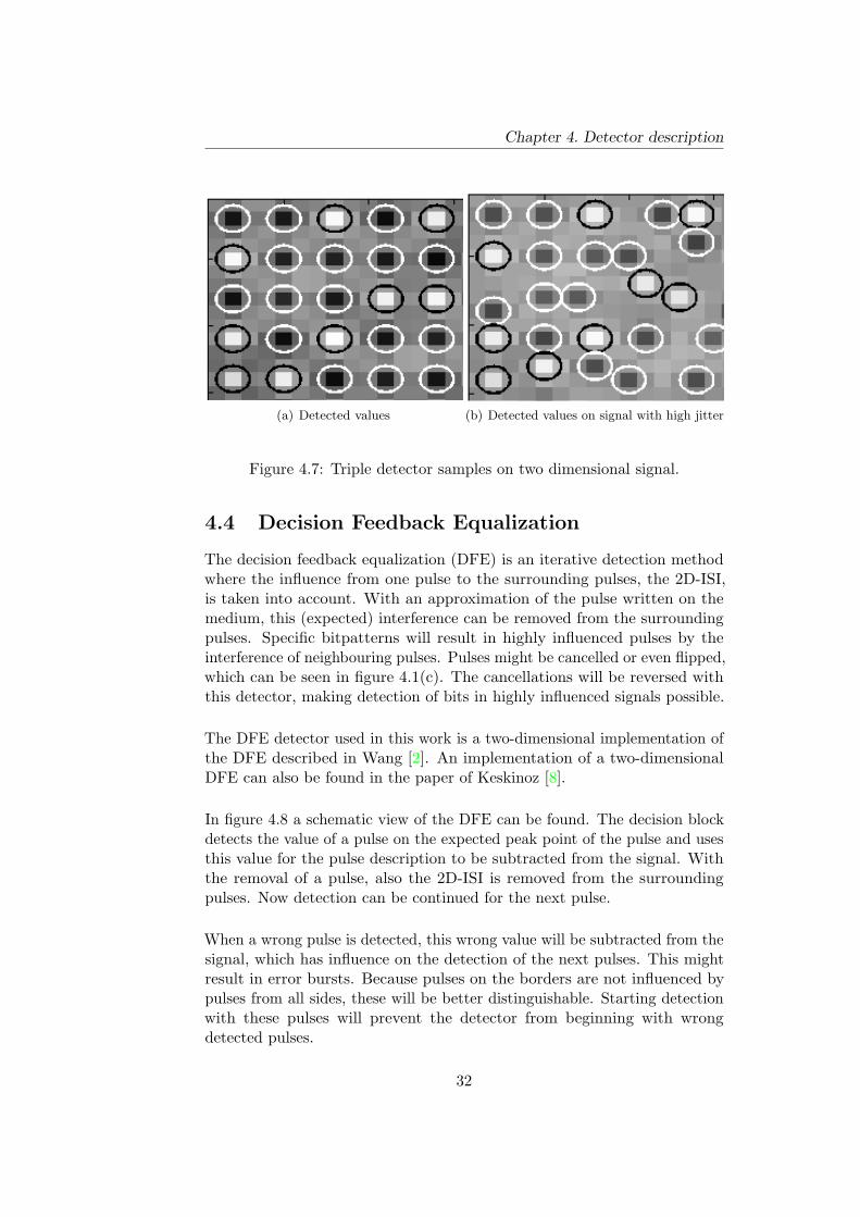
For this two-dimensional situation a 5x5 bitpattern is given in figure 4.7.Circles around the samples indicate a detected maximum. In figure 4.7(a) ajitterless signal is given and the peaks are detected on the raster. In figure4.7(b) a signal highly influenced by jitter is given, the detected maxima areindicated by the circles.
The performance of the triple detector depends a lot on the initial settingsof the detector. A change in resolution or distance between peaks withoutadapting the sample rate will influence the performance. The startpoint ofthe signal should be defined clearly, having the first signal peak within thefirst three samples. If the first value is detected wrong this might result inan error burst, causing a high bit error rate due to an error propagation.The detected bits might be right, but shifted in one or more places.
The detector can be adapted to use more or less samples per bit. Theerror rate is expected to be lower due to the higher number of samples inwhich the chance of sampling exactly on the pulse peak is higher. In thesimulations this higher sample rate is not examined, while only the conceptof this method is compared with other detectors.
31
Chapter 4. Detector description
(a) Detected values (b) Detected values on signal with high jitter
Figure 4.7: Triple detector samples on two dimensional signal.
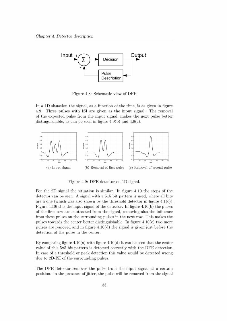
4.4 Decision Feedback Equalization
The decision feedback equalization (DFE) is an iterative detection methodwhere the influence from one pulse to the surrounding pulses, the 2D-ISI,is taken into account. With an approximation of the pulse written on themedium, this (expected) interference can be removed from the surroundingpulses. Specific bitpatterns will result in highly influenced pulses by theinterference of neighbouring pulses. Pulses might be cancelled or even flipped,which can be seen in figure 4.1(c). The cancellations will be reversed withthis detector, making detection of bits in highly influenced signals possible.
The DFE detector used in this work is a two-dimensional implementation ofthe DFE described in Wang [2]. An implementation of a two-dimensionalDFE can also be found in the paper of Keskinoz [8].
In figure 4.8 a schematic view of the DFE can be found. The decision blockdetects the value of a pulse on the expected peak point of the pulse and usesthis value for the pulse description to be subtracted from the signal. Withthe removal of a pulse, also the 2D-ISI is removed from the surroundingpulses. Now detection can be continued for the next pulse.
When a wrong pulse is detected, this wrong value will be subtracted from thesignal, which has influence on the detection of the next pulses. This mightresult in error bursts. Because pulses on the borders are not influenced bypulses from all sides, these will be better distinguishable. Starting detectionwith these pulses will prevent the detector from beginning with wrongdetected pulses.
32
Chapter 4. Detector description
Input OutputDecision
PulseDescription
!+
-
Figure 4.8: Schematic view of DFE
In a 1D situation the signal, as a function of the time, is as given in figure4.9. Three pulses with ISI are given as the input signal. The removalof the expected pulse from the input signal, makes the next pulse betterdistinguishable, as can be seen in figure 4.9(b) and 4.9(c).
0 10 20 30 40 50 60−0.4
−0.2
0
0.2
0.4
0.6
0.8
1
time
amplitude
(a) Input signal
0 10 20 30 40 50 60−0.4
−0.2
0
0.2
0.4
0.6
0.8
1
time
amplitude
(b) Removal of first pulse
0 10 20 30 40 50 60−0.4
−0.2
0
0.2
0.4
0.6
0.8
1
time
amplitude
(c) Removal of second pulse
Figure 4.9: DFE detector on 1D signal.
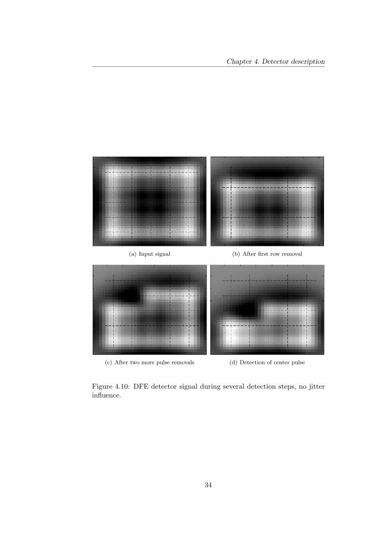
For the 2D signal the situation is similar. In figure 4.10 the steps of thedetector can be seen. A signal with a 5x5 bit pattern is used, where all bitsare a one (which was also shown by the threshold detector in figure 4.1(c)).Figure 4.10(a) is the input signal of the detector. In figure 4.10(b) the pulsesof the first row are subtracted from the signal, removing also the influencefrom these pulses on the surrounding pulses in the next row. This makes thepulses towards the center better distinguishable. In figure 4.10(c) two morepulses are removed and in figure 4.10(d) the signal is given just before thedetection of the pulse in the center.
By comparing figure 4.10(a) with figure 4.10(d) it can be seen that the centervalue of this 5x5 bit pattern is detected correctly with the DFE detection.In case of a threshold or peak detection this value would be detected wrongdue to 2D-ISI of the surrounding pulses.
The DFE detector removes the pulse from the input signal at a certainposition. In the presence of jitter, the pulse will be removed from the signal
33
Chapter 4. Detector description
(a) Input signal (b) After first row removal
(c) After two more pulse removals (d) Detection of center pulse
Figure 4.10: DFE detector signal during several detection steps, no jitterinfluence.
34
Chapter 4. Detector description
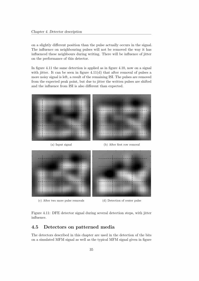
on a slightly different position than the pulse actually occurs in the signal.The influence on neighbouring pulses will not be removed the way it hasinfluenced these neighbours during writing. There will be influence of jitteron the performance of this detector.
In figure 4.11 the same detection is applied as in figure 4.10, now on a signalwith jitter. It can be seen in figure 4.11(d) that after removal of pulses amore noisy signal is left, a result of the remaining ISI. The pulses are removedfrom the expected peak point, but due to jitter the written pulses are shiftedand the influence from ISI is also different than expected.
(a) Input signal (b) After first row removal
(c) After two more pulse removals (d) Detection of center pulse
Figure 4.11: DFE detector signal during several detection steps, with jitterinfluence.
4.5 Detectors on patterned media
The detectors described in this chapter are used in the detection of the bitson a simulated MFM signal as well as the typical MFM signal given in figure
35

Chapter 4. Detector description
3.1. By varying the pulse period, signal to noise ratio, jitter and sample ratecomparisons can be made between the performances of these detectors. Theresults of these simulations are given in chapter 6.
With the variation of the pulse period, also the shape of the pulse can bevaried. By changing the shape of the pulses also the 2D-ISI changes anddetector performance is influenced. The shape variation is not taken intoaccount in the simulations. Only the comparison between detectors with onespecific pulse is taken into account.
36
Chapter 5Image Processing Techniques
In all methods described in chapter 4 impressions of the signal are shown asgrayscale images. On these images dots appear and depending on the presenceof noise and jitter, these dots are more or less distinguishable. Instead ofusing the common detection methods derived from the one-dimensionalmethods, specific image processing recognition and detection methods canbe used. The dots can be detected with object recognition algorithms andso the bit values of the input signal can be detected.
The MFM signal is built of positive and negative pulses with more or lessknown properties. These pulses are the objects to be recognized and appearas black and white dots on a gray background. The geometry of the pulsesis rotational invariant.
Different methods from the book Image Based Measurement Systems byVan der Heijden[16] are applied on the simulation of the MFM signal anddescribed in the next sections.
5.1 Spot Detection
In the signal generated in the simulation, the dots are clearly visible whendisplayed as an image. From an image processing view this looks like a spotdetection problem. A model for the description of the spot field is given inequation 5.1.
f(x, y) = C0 +∑
i
Cih(x− xi, y − yi) + n(x, y) (5.1)
37
Chapter 5. Image Processing Techniques
In this equation C0 is the background and Cih are the amplitudes of thespots on the respective (xi, yi) positions. The goal is to detect the positionsof the spots in the f(x, y) image, in which the Ci value is the value of thisbit, either −1 or 1.
It is a very obvious way to detect these pulses by comparing the image with atemplate. The template is a description of the image to be detected. A crosscorrelation can be calculated between the input image and the template.This cross correlation information can be used in a detector where values onspecific positions will exceed a threshold, defining the position of the spot.
In terms of image processing the process for the spot detection now exists oftwo parts: Feature extraction and classification.
5.2 Feature extraction
Goal of the algorithms is finding the dots in the image. These dots havecertain properties, called features. By extracting these features from theMFM signal, and so reducing the disturbances in the signal, the relevantinformation is left over for detection.
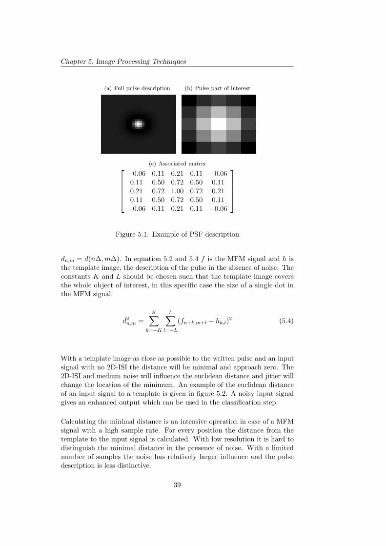
5.2.1 Point spread function
The point spread function (PSF) of the pulses is described in chapter 3 asthe pulse description of the simulation signal. This same function can beused in the image processing detection mechanisms for comparison with theinput signal. The resolution of the PSF is depending on the resolution of thedots in the MFM signal. An example of the PSF and the associated matrixis given in figure 5.1.
5.2.2 Euclidean Distance
By comparing the MFM signal with a template, a distance can be calculatedbetween these two signals. The position of the template on the signal withthe smallest distance is the expected position for a peak. This comparisoncan be done with the euclidean distance between the image and the template.The calculation for the distance is given in equation 5.2.
d2(ξ, η) =∫∫
x,y(f(x, y)− h(x− ξ, y− η))2 d(ξ̂, η̂) = min{d(ξ, η)} (5.2)
Which can be written as
d2(ξ, η) =∫∫
x,y(f(x+ ξ, y + η)− h(x, y))2 (5.3)
The discrete case is given is equation 5.4, where d2(ξ, η) corresponds to
38
Chapter 5. Image Processing Techniques
(a) Full pulse description (b) Pulse part of interest
(c) Associated matrix−0.06 0.11 0.21 0.11 −0.060.11 0.50 0.72 0.50 0.110.21 0.72 1.00 0.72 0.210.11 0.50 0.72 0.50 0.11−0.06 0.11 0.21 0.11 −0.06
Figure 5.1: Example of PSF description
dn,m = d(n∆,m∆). In equation 5.2 and 5.4 f is the MFM signal and h isthe template image, the description of the pulse in the absence of noise. Theconstants K and L should be chosen such that the template image coversthe whole object of interest, in this specific case the size of a single dot inthe MFM signal.
d2n,m =
K∑k=−K
L∑l=−L
(fn+k,m+l − hk,l)2 (5.4)
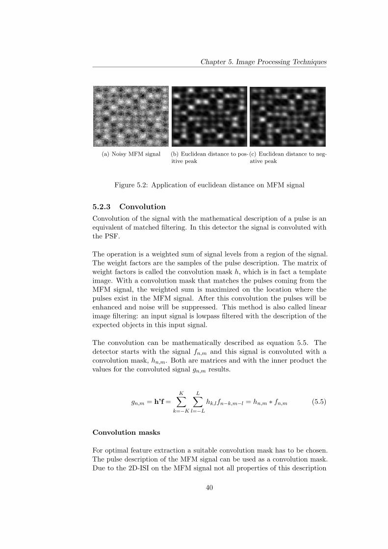
With a template image as close as possible to the written pulse and an inputsignal with no 2D-ISI the distance will be minimal and approach zero. The2D-ISI and medium noise will influence the euclidean distance and jitter willchange the location of the minimum. An example of the euclidean distanceof an input signal to a template is given in figure 5.2. A noisy input signalgives an enhanced output which can be used in the classification step.
Calculating the minimal distance is an intensive operation in case of a MFMsignal with a high sample rate. For every position the distance from thetemplate to the input signal is calculated. With low resolution it is hard todistinguish the minimal distance in the presence of noise. With a limitednumber of samples the noise has relatively larger influence and the pulsedescription is less distinctive.
39
Chapter 5. Image Processing Techniques
(a) Noisy MFM signal (b) Euclidean distance to pos-itive peak
(c) Euclidean distance to neg-ative peak
Figure 5.2: Application of euclidean distance on MFM signal
5.2.3 Convolution
Convolution of the signal with the mathematical description of a pulse is anequivalent of matched filtering. In this detector the signal is convoluted withthe PSF.
The operation is a weighted sum of signal levels from a region of the signal.The weight factors are the samples of the pulse description. The matrix ofweight factors is called the convolution mask h, which is in fact a templateimage. With a convolution mask that matches the pulses coming from theMFM signal, the weighted sum is maximized on the location where thepulses exist in the MFM signal. After this convolution the pulses will beenhanced and noise will be suppressed. This method is also called linearimage filtering: an input signal is lowpass filtered with the description of theexpected objects in this input signal.
The convolution can be mathematically described as equation 5.5. Thedetector starts with the signal fn,m and this signal is convoluted with aconvolution mask, hn,m. Both are matrices and with the inner product thevalues for the convoluted signal gn,m results.
gn,m = h’f =K∑
k=−K
L∑l=−L
hk,lfn−k,m−l = hn,m ∗ fn,m (5.5)
Convolution masks
For optimal feature extraction a suitable convolution mask has to be chosen.The pulse description of the MFM signal can be used as a convolution mask.Due to the 2D-ISI on the MFM signal not all properties of this description
40
Chapter 5. Image Processing Techniques
will be visible, for example the undershoot of the pulse, which is overlappingwith the neighbouring pulses. An adapted convolution mask can give similarresults with a reduced number of calculations.
A gaussian pulse can be used as a convolution mask. In equation 5.6 thedescription for a gaussian pulse is given.
hx,y = Ae−(
(x−x0)2
2σ2x
+(y−y0)2
2σ2y
)(5.6)
Where A is the amplitude of the pulse. x0 and y0 the centers of the pulseand σx and σy the x and y spreads.
This pulse as convolution mask can easily be adapted from a circular toelliptical form by using different values for σx and σy. Examples of convolutionmasks created by a gaussian pulse are given in figure 5.3. In figure 5.3(c) alsoa rotated mask can be found. In case of the typical MFM signal example givenin section 3.4.4 this mask can be used before rotation and transformation ofthe signal is applied.
(a) Circular Gaussian convo-lution mask
(b) Elliptical convolutionmask
(c) Rotated elliptical convolu-tion mask
Figure 5.3: Examples of convolution masks
Applying convolution masks
In figure 5.4 the output signals can be found after applying various convolutionmasks. The MFM signal is given in figure 5.4(a). After convolution withan 8x8 mask of the pulse description of section 3.3.2 the output is givenin figure 5.4(b). Figure 5.4(c) shows the output after convolution with agaussian description for the convolution mask as a 5x5 matrix.
The figure with the Gaussian mask indicates that not an exact descriptionof the written pulse is necessary for this feature extraction. A smaller maskcan already enhance the signal and save computation power.
41
Chapter 5. Image Processing Techniques
In figure 5.5 the result of applying convolution on a noisy MFM signal witha bit pattern of 5x5 ones can be found. The output after convolution is givenin figure 5.5(b). The black dots that occur as a result of the 2D-ISI still existand may cause problems in the classification.
(a) Simulated MFM Outputsignal
(b) Convolution with pulse de-scription
(c) Convolution with gausspulse
Figure 5.4: Applying different convolution masks
(a) Noisy MFM signal of 5x5 ones (b) Convolution output of 5x5 ones
Figure 5.5: Applying convolution on noisy 5x5 ones
Image border effects
When a convolution is applied, there will occur irregularities on the borders.An example can be seen in figure 5.6. In figure 5.6(b) a disturbance of thebits on all borders is visible.
It is a common problem with convolution, which can be solved by paddingthe border with the same values as the background, usually zero’s. In thesimulations the signal is created with a wide border preventing the occurrenceof such effects in the convolution. After the convolution the padding can beremoved before further processing. In figure 5.6(c) a padding with zero’s
42
Chapter 5. Image Processing Techniques
has been applied and pulses on the borders are not disturbed by the bordereffect anymore.
20 40 60 80 100 120 140 160 180 200
20
40
60
80
100
120
140
160
180
200 (a) Simulated MFM Outputsignal
20 40 60 80 100 120 140
20
40
60
80
100
120
140
(b) Convolution withoutpadding with zero’s 20 40 60 80 100 120 140 160 180 200
20
40
60
80
100
120
140
160
180
200 (c) Convolution with padding
Figure 5.6: Border effects with convolution
5.2.4 Laplacian of the Gaussian
On the signal after convolution the Laplace operator can be applied. TheLaplacian is the second order derivative, given in equation 5.7.
∆f = ∇2f =δ2f
δx2+δ2f
δy2(5.7)
The result of this operator on a signal after convolution is a strong responson the positions for the black and white dots on the MFM signal. In figure5.7(b) the result of this operator applied on figure 5.7(a) can be found.
(a) Convoluted MFM signal (b) After application of Laplacian
Figure 5.7: Signal before and after laplacian.
43
Chapter 5. Image Processing Techniques
5.3 Classification
After the feature extraction methods the dots in the signal are enhanced.The next step is to localize the dots in the signal and decide whether or notthey are a written pulse or a result of ISI and ITI.
5.3.1 Non-local maximum suppression
Besides a way of detecting pulses, there is also the problem of the localizationof the pulses. In an ideal situation the detector should be able to localizethe pulses, making the use of a clock unnecessary. A non-local maximumsuppression algorithm is a method for solving this problem. As the namesays, it is a suppression of the non-local maxima. At the output of thisalgorithm the local maxima are still available, representing the pulses of thesignal. With this algorithm the influence of jitter is also minimized.
In the MFM signal, matrix f , there are positive and negative peaks. Tomake all dots positive the absolute value of the signal is taken, resultingin fabs. Now for all samples in the signal a comparison can be made withthe neighbouring values. When a sample is larger than the samples in itsdirect surrounding and above the threshold value, the position is classifiedas a peak. The output matrix fout now consists of values −1 or 1 on peakpositions and 0 elsewhere. The algorithm of this method is given in listing 5.1.
f_abs = abs(f);f_out = zeros(size(f));threshold = THD;for i = 1: rowSamples
for j = 1: colSamplesif ((( f_abs(i,j) >= f_abs(i-1,j)) && ...
(f_abs(i,j) >= f_abs(i+1,j)) && ...(f_abs(i,j) >= f_abs(i,j-1)) && ...(f_abs(i,j) >= f_abs(i,j+1))) && ...(f_abs(i,j) >= f_abs(i-1,j-1)) && ...(f_abs(i,j) >= f_abs(i+1,j+1)) && ...(f_abs(i,j) >= f_abs(i+1,j-1)) && ...(f_abs(i,j) >= f_abs(i-1,j+1)) )if(f_abs(i,j) > threshold ))
f_out(i,j) = sign(f(i,j));end
elsef_out(i,j) = 0;
endend
end
Listing 5.1: Local Maximum Suppression algorithm in Matlab
44
Chapter 5. Image Processing Techniques
The number of samples in the surrounding which is taken into account canbe varied. Depending on the size, the sample rate and the period of the dotson the signal.
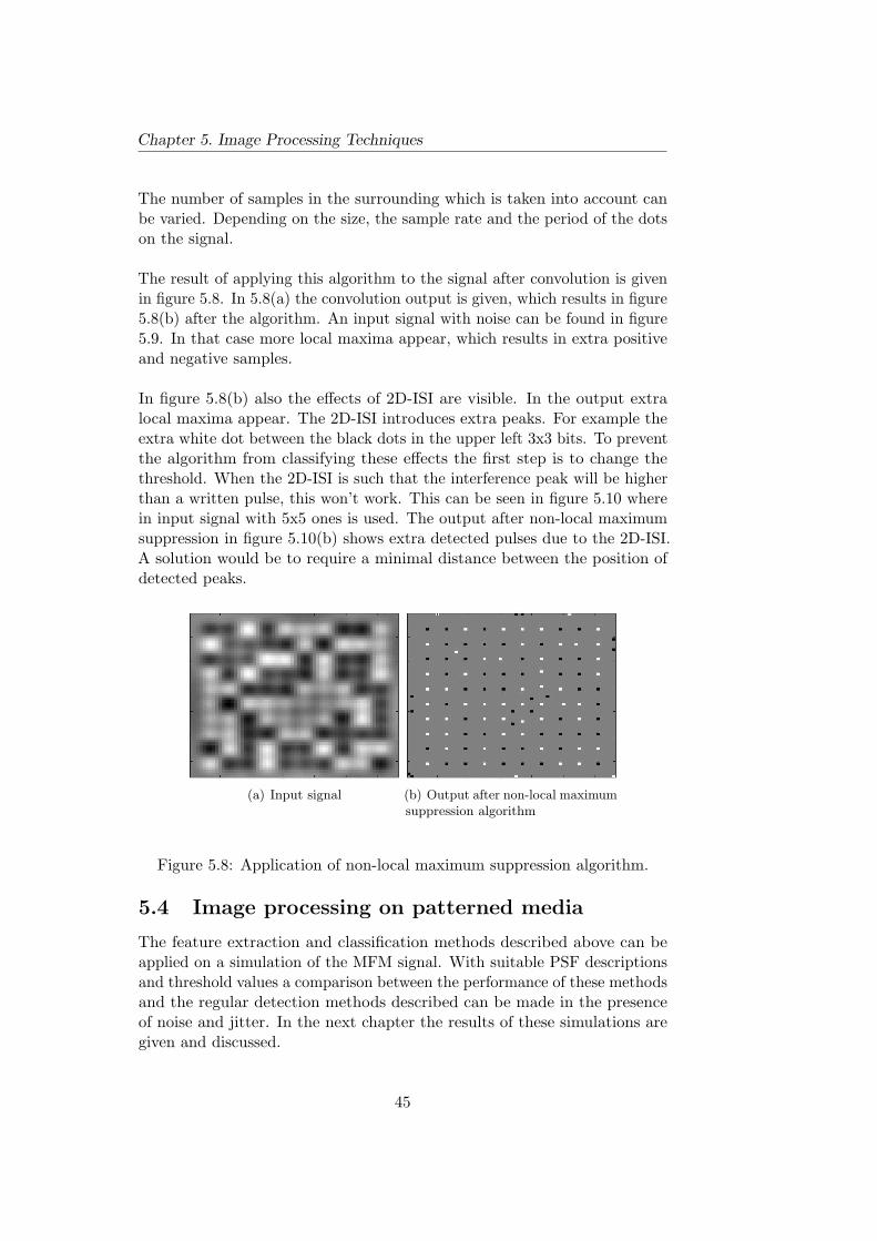
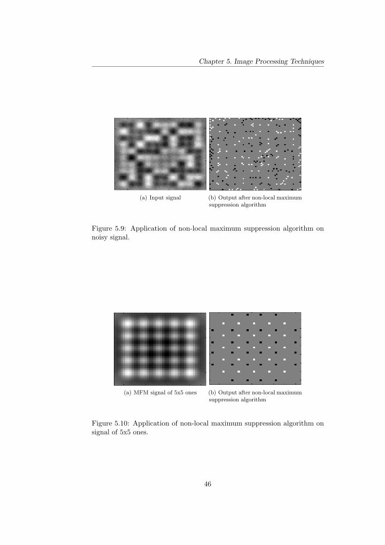
The result of applying this algorithm to the signal after convolution is givenin figure 5.8. In 5.8(a) the convolution output is given, which results in figure5.8(b) after the algorithm. An input signal with noise can be found in figure5.9. In that case more local maxima appear, which results in extra positiveand negative samples.
In figure 5.8(b) also the effects of 2D-ISI are visible. In the output extralocal maxima appear. The 2D-ISI introduces extra peaks. For example theextra white dot between the black dots in the upper left 3x3 bits. To preventthe algorithm from classifying these effects the first step is to change thethreshold. When the 2D-ISI is such that the interference peak will be higherthan a written pulse, this won’t work. This can be seen in figure 5.10 wherein input signal with 5x5 ones is used. The output after non-local maximumsuppression in figure 5.10(b) shows extra detected pulses due to the 2D-ISI.A solution would be to require a minimal distance between the position ofdetected peaks.
(a) Input signal (b) Output after non-local maximumsuppression algorithm
Figure 5.8: Application of non-local maximum suppression algorithm.
5.4 Image processing on patterned media
The feature extraction and classification methods described above can beapplied on a simulation of the MFM signal. With suitable PSF descriptionsand threshold values a comparison between the performance of these methodsand the regular detection methods described can be made in the presenceof noise and jitter. In the next chapter the results of these simulations aregiven and discussed.
45
Chapter 5. Image Processing Techniques
(a) Input signal (b) Output after non-local maximumsuppression algorithm
Figure 5.9: Application of non-local maximum suppression algorithm onnoisy signal.
(a) MFM signal of 5x5 ones (b) Output after non-local maximumsuppression algorithm
Figure 5.10: Application of non-local maximum suppression algorithm onsignal of 5x5 ones.
46

Chapter 6Results and Discussion
This chapter gives the results of the different detectors with different influencefrom jitter and medium noise. The simulations are done with the pulsedescription given in chapter 3 with an input matrix of 25x25 bits. The signalis simulated with varying sample rates and pulse periods. On the bordersthe pulses are not influenced from all sides, as described in section 3.4.5.By removing two bits on all sides a number of databits of 23x23 bits isused in each simulation signal. This signal is generated many times with apseudorandom bitpattern.
In conventional storage media a raw bit error rate of 10−4 is the maximumfor a detector to be useful in detection. For the simulations in this workthis is also the guideline. If in a series of simulations no errors occur thisdoesn’t mean the bit error rate is zero. It just means that not enough bitsare simulated to detect the errors. However, also detecting only a few errorswith a big number of simulations is no measurement for a low BER. Beforethe BER is statistically significant at least 100 errors have to be detected.This means for a statistically significant BER of 10−4 at least one millionbits have to be simulated.
6.1 Patterned media simulations
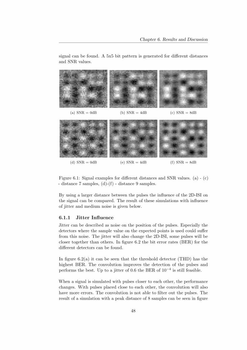
For the simulations a bit pattern is generated with individual pulses of 15x15samples, where the pulse includes the overshoot. These pulses are placedwith a pulse period of 7 to 9 samples from peak to peak. In the case of 7samples a peak wil be exactly on the overshoot peak of a neighbouring pulse.The 2D-ISI is maximized in that case. In figure 6.1 the examples of this
47
Chapter 6. Results and Discussion
signal can be found. A 5x5 bit pattern is generated for different distancesand SNR values.
(a) SNR = 0dB (b) SNR = 4dB (c) SNR = 8dB
(d) SNR = 0dB (e) SNR = 4dB (f) SNR = 8dB
Figure 6.1: Signal examples for different distances and SNR values. (a) - (c)- distance 7 samples, (d)-(f) - distance 9 samples.
By using a larger distance between the pulses the influence of the 2D-ISI onthe signal can be compared. The result of these simulations with influenceof jitter and medium noise is given below.
6.1.1 Jitter Influence
Jitter can be described as noise on the position of the pulses. Especially thedetectors where the sample value on the expected points is used could sufferfrom this noise. The jitter will also change the 2D-ISI, some pulses will becloser together than others. In figure 6.2 the bit error rates (BER) for thedifferent detectors can be found.
In figure 6.2(a) it can be seen that the threshold detector (THD) has thehighest BER. The convolution improves the detection of the pulses andperforms the best. Up to a jitter of 0.6 the BER of 10−4 is still feasible.
When a signal is simulated with pulses closer to each other, the performancechanges. With pulses placed close to each other, the convolution will alsohave more errors. The convolution is not able to filter out the pulses. Theresult of a simulation with a peak distance of 8 samples can be seen in figure
48
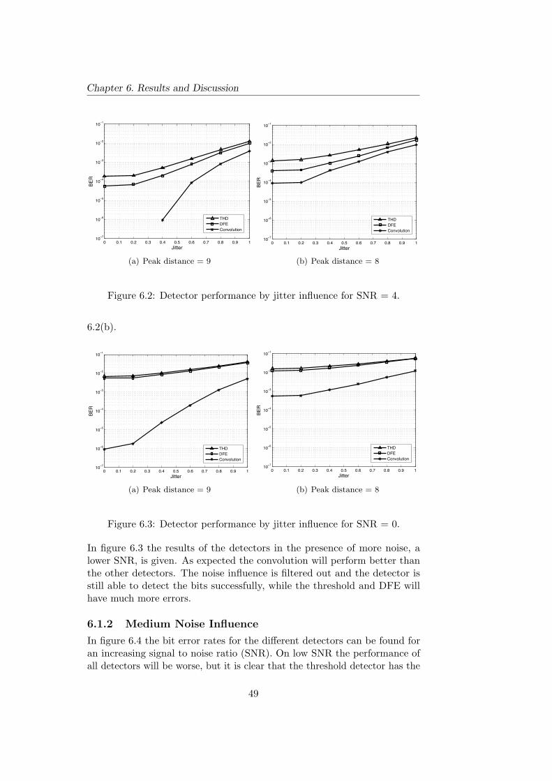
Chapter 6. Results and Discussion
0 0.1 0.2 0.3 0.4 0.5 0.6 0.7 0.8 0.9 110−7
10−6
10−5
10−4
10−3
10−2
10−1
Jitter
BER
THDDFEConvolution
(a) Peak distance = 9
0 0.1 0.2 0.3 0.4 0.5 0.6 0.7 0.8 0.9 110−7
10−6
10−5
10−4
10−3
10−2
10−1
Jitter
BER
THDDFEConvolution
(b) Peak distance = 8
Figure 6.2: Detector performance by jitter influence for SNR = 4.
6.2(b).
0 0.1 0.2 0.3 0.4 0.5 0.6 0.7 0.8 0.9 110−7
10−6
10−5
10−4
10−3
10−2
10−1
Jitter
BER
THDDFEConvolution
(a) Peak distance = 9
0 0.1 0.2 0.3 0.4 0.5 0.6 0.7 0.8 0.9 110−7
10−6
10−5
10−4
10−3
10−2
10−1
Jitter
BER
THDDFEConvolution
(b) Peak distance = 8
Figure 6.3: Detector performance by jitter influence for SNR = 0.
In figure 6.3 the results of the detectors in the presence of more noise, alower SNR, is given. As expected the convolution will perform better thanthe other detectors. The noise influence is filtered out and the detector isstill able to detect the bits successfully, while the threshold and DFE willhave much more errors.
6.1.2 Medium Noise Influence
In figure 6.4 the bit error rates for the different detectors can be found foran increasing signal to noise ratio (SNR). On low SNR the performance ofall detectors will be worse, but it is clear that the threshold detector has the
49
Chapter 6. Results and Discussion
same behaviour as can be seen in the jitter plots. The performance won’t getbetter above a certain SNR, due to the worst-case patterns in the signal.
0 2 4 6 8 10 12 14 16 18 2010−7
10−6
10−5
10−4
10−3
10−2
10−1
SNR (dB)
BER
THDDFEConvolution
(a) Pulse distance = 8
0 2 4 6 8 10 12 14 16 18 2010−7
10−6
10−5
10−4
10−3
10−2
10−1
SNR (dB)
BER
THDDFEConvolution
(b) Pulse distance = 7
Figure 6.4: Detector performance by medium noise.
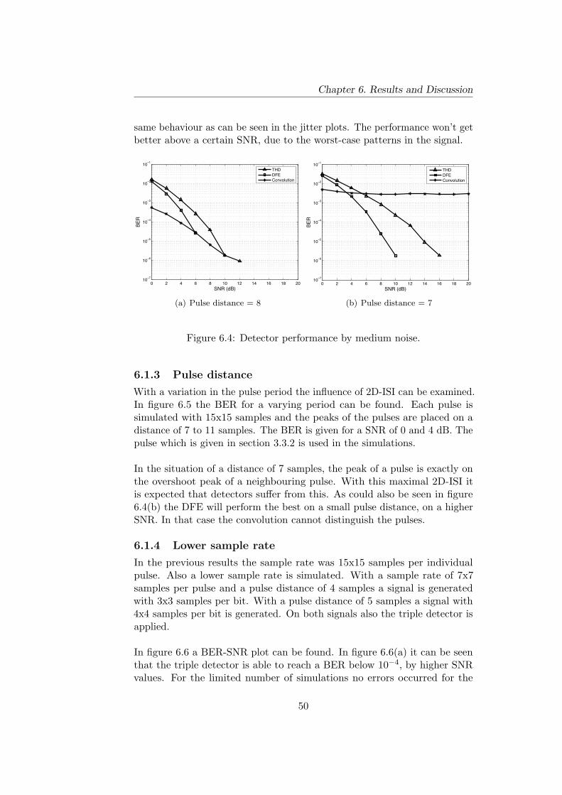
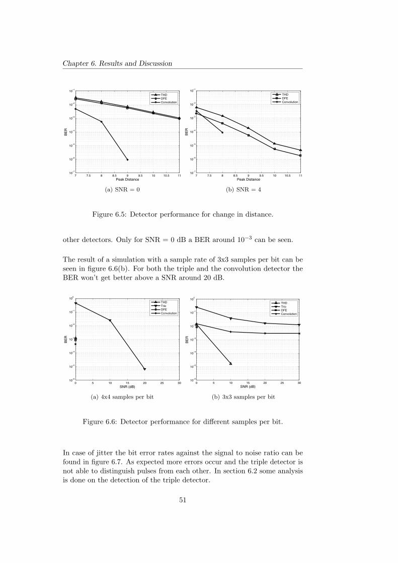
6.1.3 Pulse distance
With a variation in the pulse period the influence of 2D-ISI can be examined.In figure 6.5 the BER for a varying period can be found. Each pulse issimulated with 15x15 samples and the peaks of the pulses are placed on adistance of 7 to 11 samples. The BER is given for a SNR of 0 and 4 dB. Thepulse which is given in section 3.3.2 is used in the simulations.
In the situation of a distance of 7 samples, the peak of a pulse is exactly onthe overshoot peak of a neighbouring pulse. With this maximal 2D-ISI itis expected that detectors suffer from this. As could also be seen in figure6.4(b) the DFE will perform the best on a small pulse distance, on a higherSNR. In that case the convolution cannot distinguish the pulses.
6.1.4 Lower sample rate
In the previous results the sample rate was 15x15 samples per individualpulse. Also a lower sample rate is simulated. With a sample rate of 7x7samples per pulse and a pulse distance of 4 samples a signal is generatedwith 3x3 samples per bit. With a pulse distance of 5 samples a signal with4x4 samples per bit is generated. On both signals also the triple detector isapplied.
In figure 6.6 a BER-SNR plot can be found. In figure 6.6(a) it can be seenthat the triple detector is able to reach a BER below 10−4, by higher SNRvalues. For the limited number of simulations no errors occurred for the
50
Chapter 6. Results and Discussion
7 7.5 8 8.5 9 9.5 10 10.5 1110−7
10−6
10−5
10−4
10−3
10−2
10−1
Peak Distance
BER
THDDFEConvolution
(a) SNR = 0
7 7.5 8 8.5 9 9.5 10 10.5 1110−7
10−6
10−5
10−4
10−3
10−2
10−1
Peak DistanceBE
R
THDDFEConvolution
(b) SNR = 4
Figure 6.5: Detector performance for change in distance.
other detectors. Only for SNR = 0 dB a BER around 10−3 can be seen.
The result of a simulation with a sample rate of 3x3 samples per bit can beseen in figure 6.6(b). For both the triple and the convolution detector theBER won’t get better above a SNR around 20 dB.
0 5 10 15 20 25 3010−6
10−5
10−4
10−3
10−2
10−1
100
SNR (dB)
BER
THDTrioDFEConvolution
(a) 4x4 samples per bit
0 5 10 15 20 25 3010−6
10−5
10−4
10−3
10−2
10−1
100
SNR (dB)
BER
THDTrioDFEConvolution
(b) 3x3 samples per bit
Figure 6.6: Detector performance for different samples per bit.
In case of jitter the bit error rates against the signal to noise ratio can befound in figure 6.7. As expected more errors occur and the triple detector isnot able to distinguish pulses from each other. In section 6.2 some analysisis done on the detection of the triple detector.
51
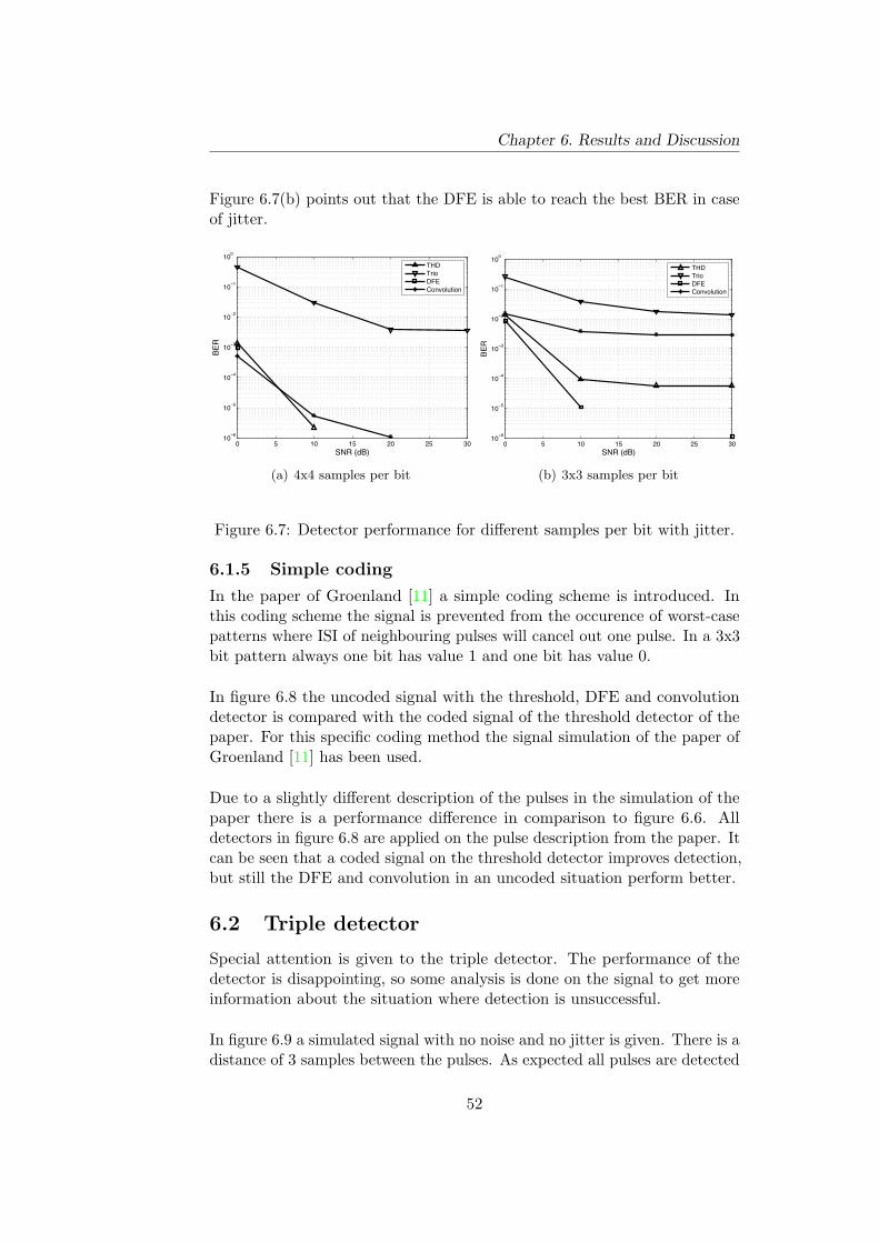
Chapter 6. Results and Discussion
Figure 6.7(b) points out that the DFE is able to reach the best BER in caseof jitter.
0 5 10 15 20 25 3010−6
10−5
10−4
10−3
10−2
10−1
100
SNR (dB)
BER
THDTrioDFEConvolution
(a) 4x4 samples per bit
0 5 10 15 20 25 3010−6
10−5
10−4
10−3
10−2
10−1
100
SNR (dB)
BER
THDTrioDFEConvolution
(b) 3x3 samples per bit
Figure 6.7: Detector performance for different samples per bit with jitter.
6.1.5 Simple coding
In the paper of Groenland [11] a simple coding scheme is introduced. Inthis coding scheme the signal is prevented from the occurence of worst-casepatterns where ISI of neighbouring pulses will cancel out one pulse. In a 3x3bit pattern always one bit has value 1 and one bit has value 0.
In figure 6.8 the uncoded signal with the threshold, DFE and convolutiondetector is compared with the coded signal of the threshold detector of thepaper. For this specific coding method the signal simulation of the paper ofGroenland [11] has been used.
Due to a slightly different description of the pulses in the simulation of thepaper there is a performance difference in comparison to figure 6.6. Alldetectors in figure 6.8 are applied on the pulse description from the paper. Itcan be seen that a coded signal on the threshold detector improves detection,but still the DFE and convolution in an uncoded situation perform better.
6.2 Triple detector
Special attention is given to the triple detector. The performance of thedetector is disappointing, so some analysis is done on the signal to get moreinformation about the situation where detection is unsuccessful.
In figure 6.9 a simulated signal with no noise and no jitter is given. There is adistance of 3 samples between the pulses. As expected all pulses are detected
52
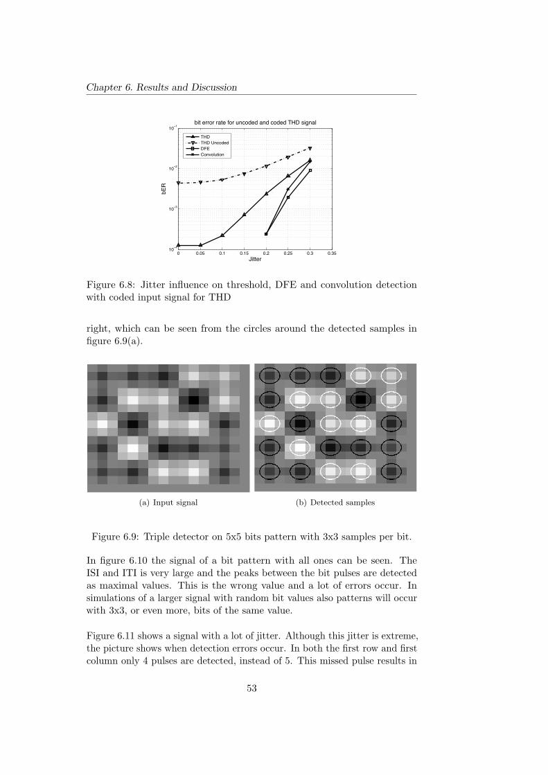
Chapter 6. Results and Discussion
0 0.05 0.1 0.15 0.2 0.25 0.3 0.3510−4
10−3
10−2
10−1
Jitter
bER
bit error rate for uncoded and coded THD signal
THDTHD UncodedDFEConvolution
Figure 6.8: Jitter influence on threshold, DFE and convolution detectionwith coded input signal for THD
right, which can be seen from the circles around the detected samples infigure 6.9(a).
(a) Input signal (b) Detected samples
Figure 6.9: Triple detector on 5x5 bits pattern with 3x3 samples per bit.
In figure 6.10 the signal of a bit pattern with all ones can be seen. TheISI and ITI is very large and the peaks between the bit pulses are detectedas maximal values. This is the wrong value and a lot of errors occur. Insimulations of a larger signal with random bit values also patterns will occurwith 3x3, or even more, bits of the same value.
Figure 6.11 shows a signal with a lot of jitter. Although this jitter is extreme,the picture shows when detection errors occur. In both the first row and firstcolumn only 4 pulses are detected, instead of 5. This missed pulse results in
53
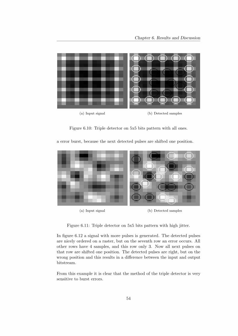
Chapter 6. Results and Discussion
(a) Input signal (b) Detected samples
Figure 6.10: Triple detector on 5x5 bits pattern with all ones.
a error burst, because the next detected pulses are shifted one position.
(a) Input signal (b) Detected samples
Figure 6.11: Triple detector on 5x5 bits pattern with high jitter.
In figure 6.12 a signal with more pulses is generated. The detected pulsesare nicely ordered on a raster, but on the seventh row an error occurs. Allother rows have 4 samples, and this row only 3. Now all next pulses onthat row are shifted one position. The detected pulses are right, but on thewrong position and this results in a difference between the input and outputbitstream.
From this example it is clear that the method of the triple detector is verysensitive to burst errors.
54

Chapter 6. Results and Discussion
(a) Input signal (b) Detected samples
Figure 6.12: Triple detector on 15x15 bits pattern.
55

Chapter 6. Results and Discussion
56

Chapter 7Conclusions andRecommendations
7.1 Conclusions
Different detectors have been investigated on random patterns with jitterand medium noise. The error rates of the detectors have been comparedresulting in the following conclusions.
7.1.1 Detector performance
For the situation with jitter on the received signal, the decision feedback equal-ization and convolution detectors perform better than the simple thresholddetector. The threshold detector always will have errors due to the worst-case patterns, where a pulse is surrounded by pulses of the same sign. Thispresence of those patterns is of less influence with the other detectors. Inthe DFE the influences from surrounding pulses are removed and with theconvolution the signal is filtered, which enhances the pulses and makes aninfluenced pulse better visible for detection.
The performance of the convolution detector is the worst in case of pulsesclose to each other. In that case the pulses can’t be distinguished anddetection fails.
7.1.2 Detector choice
The choice of a more intelligent detector will result in a lower error rate onthe detection of the pulses especially in the case of jitter and low medium
57

Chapter 7. Conclusions and Recommendations
noise. Because the pulse description of the signal is known it is possible touse this information in the detection. The more computation power neededfor detection also has to be taken into account before a detector can belabeled as better. Its performance improvement has to be higher than thefactor of extra computation power needed for the detection.
In this work it turned out that the DFE detection performs best with a smallpulse period. In the case of a bigger pulse period the convolution can handlethe most jitter and noise. An error rate of 10−2 with the threshold detectoris reduced to 10−6 with the convolution detector, taking about a 100 timesmore computation power.
7.1.3 Coding
For the simple threshold also used in the paper [11] the use of a relativesimple coding scheme already lowers the error rate. For the detectors withDFE and Convolution this difference is much smaller. The use of a codingscheme than lowers the bit-density which is not compensated by a reductionof errors.
The use of another coding scheme which is designed to prevent the worst-casepatterns for the DFE and convolution detectors might improve the detection.In this work no further research has been done to this worst-case patterns.
7.1.4 Computation Power
While the image processing techniques perform better than the regularmethods, this also has its cost. The DFE and convolution need morecomputations for the detection of a pulse. In the MatLab simulations itturned out that these simulations take up to a 100 times more computationpower, resulting in an error rate which is, even in case of jitter, several ordersof magnitude lower than with just threshold detection. This increase ofcomputation power is compensated by the improvement in error detection.
7.2 Recommendations
7.2.1 Worst-case patterns
In the detection with the simple threshold it turned out that there are arelative big number of errors in the case of no jitter. From the work donewithin the TST-SMI group it turned out this is due to worst-case patternsin which a pulse is cancelled by the influence from its surrounding. For theother detectors the error rate is very low in the case of no jitter, but it isunknown what the exact reason is for these errors. This might be related toworst-case patterns and can be researched further.
58

Chapter 7. Conclusions and Recommendations
7.2.2 Computation Power
A more intelligent detector also needs more computation power. In thisresearch the difference between computation power has only taken intoaccount by comparing the time needed for the calculations in MatLab. Therecan be done more research on this comparison in order to conclude if thecomputations for a detector are worth the improvement on the error rate.
7.2.3 Non-linear signal patterns
The detected signal coming from the MFM is not directly usable in thedetector due to non linearities of the readout, like a rotation and perspective,which can be seen when shown as an image. With image processing tools thiscan be compensated before any detection is applied. It should be studied ifit is possible to convert the signal in such a way that the linear detectionmethods which are used in this work can be used directly.
In a paper of Tang et. al. [15] a technique is described for write synchroniza-tion in a bit patterned medium. The synchronization is performed on a diskdrive and a spin stand comparable to writing to a disk. Although this is notthe same as bit patterned media, the technique could be useful.
7.2.4 Image Processing
As expected the convolution detector has a performance which is betterthan a simple threshold method, but the image processing field has moretechniques and between these methods also variations occur. In this workonly the convolution has been done with the description of one signal pulse,whether it might also be possible to use other filter descriptions with forexample more than one pulse included, which might improve the detectionof the signal.
7.2.5 Bits on signal border
In the simulations it turned out that the pulses on the border of the fieldshould not be used in the calculation of the error rate. The pulses on theborder are not disturbed by influence from all directions. In the simulationsit is important to remove this surrounding and only use the databits.
7.2.6 Hexagonal Pattern
A change in the ordering of the bits in the pattern gives another description ofthe 2D-ISI. With a hexagonal pattern the distance to all direct neighbouringpulses will be equal, so also the 2D-ISI from all pulses will be equal. Thiswill influence the detection rates and might result in a higher bit density byplacing the pulses closer to each other.
59

Chapter 7. Conclusions and Recommendations
60
Appendix ASimulator and detector code
In this appendix the code for the signal simulation and the detectors is given.
A.1 Signal Simulation
A.1.1 Pulse generator
1 function pulse = pulse2d(pulselength , amplitude , pw50 , origins , noise)
2 % Create a lorentzpulse
3 %
4 % Input:
5 % pulselength (resolution),
6 % amplitudes [a1 a2 a3],
7 % pw50 [p1 p2 p3],
8 % origins [o1 o2 o3]
9 % Output:
10 % two dimensional matrix with pulse of size pulselength
11 % (or plot if no output is asked on function call)
12
13 % Set variables if not given as input
14 if nargin < 2, amplitude = [-1.1 2.45 -1.1]; end
15 if nargin < 3, pw50 = [1.9 1.9 1.9]; end
16 if nargin < 4, origins = [-0.7 0 0.7]; end
17 if nargin < 5, noise = 0; end % Noise is given as the variance
18 if nargin < 1, pulselength = 61; end
19
20 % make empty matrix
21 [X,Y] = meshgrid(-floor(pulselength /2):1: floor(pulselength /2));
22 R = sqrt(X.^2 + Y.^2);
23 lorentz = zeros(size(R));
24
25 % Combine 3 lorentzpulses
61
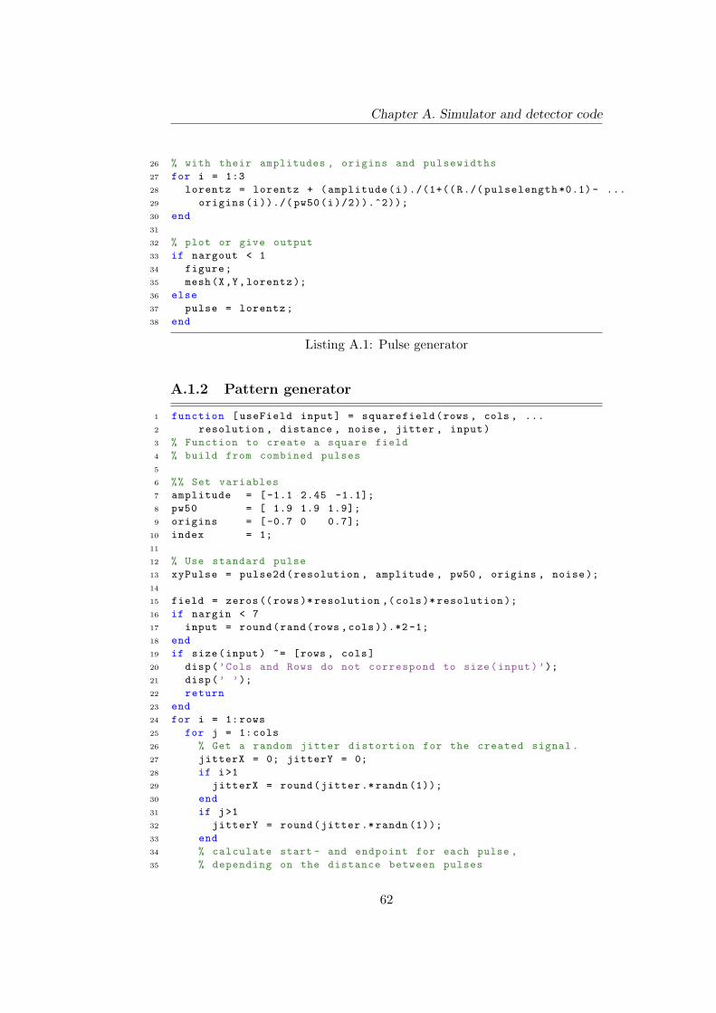
Chapter A. Simulator and detector code
26 % with their amplitudes , origins and pulsewidths
27 for i = 1:3
28 lorentz = lorentz + (amplitude(i)./(1+((R./( pulselength *0.1)- ...
29 origins(i))./( pw50(i)/2)).^2));
30 end
31
32 % plot or give output
33 if nargout < 1
34 figure;
35 mesh(X,Y,lorentz );
36 else
37 pulse = lorentz;
38 end
Listing A.1: Pulse generator
A.1.2 Pattern generator
1 function [useField input] = squarefield(rows , cols , ...
2 resolution , distance , noise , jitter , input)
3 % Function to create a square field
4 % build from combined pulses
5
6 %% Set variables
7 amplitude = [-1.1 2.45 -1.1];
8 pw50 = [ 1.9 1.9 1.9];
9 origins = [-0.7 0 0.7];
10 index = 1;
11
12 % Use standard pulse
13 xyPulse = pulse2d(resolution , amplitude , pw50 , origins , noise);
14
15 field = zeros((rows)* resolution ,(cols)* resolution );
16 if nargin < 7
17 input = round(rand(rows ,cols )).*2 -1;
18 end
19 if size(input) ~= [rows , cols]
20 disp(’Cols and Rows do not correspond to size(input)’);
21 disp(’ ’);
22 return
23 end
24 for i = 1:rows
25 for j = 1:cols
26 % Get a random jitter distortion for the created signal.
27 jitterX = 0; jitterY = 0;
28 if i>1
29 jitterX = round(jitter .* randn (1));
30 end
31 if j>1
32 jitterY = round(jitter .* randn (1));
33 end
34 % calculate start - and endpoint for each pulse ,
35 % depending on the distance between pulses
62
Chapter A. Simulator and detector code
36 % and jitter influence
37 startPointX = (i-1)* resolution +1-((i-1)* distance )+ jitterX;
38 endPointX = i*resolution -((i-1)* distance )+ jitterX;
39 startPointY = (j-1)* resolution +1-((j-1)* distance )+ jitterY;
40 endPointY = j*resolution -((j-1)* distance )+ jitterY;
41 % generate noise
42 ruis = noise .*randn(endPointX -startPointX +1,endPointY -startPointY +1);
43 % Add pulse and noise to signal (on calculated positions
44 field(startPointX:endPointX ,startPointY:endPointY) = ...
45 field(startPointX:endPointX ,startPointY:endPointY) + ...
46 input(i,j)* xyPulse + ruis;
47 end
48 end
49 useField = zeros(j*resolution -((j-1)* distance),i*resolution -((i-1)* distance ));
50 useField (1: endPointY , 1: endPointX) = field (1: endPointY , 1: endPointX );
51
52 % Plot an image of the generated field
53 % only if not output matrix is asked
54 if nargout == 0
55 colormap(gray)
56 imagesc(useField );
57 end
Listing A.2: Pattern Generator
A.2 Detectors
A.2.1 Threshold detector
1 function [output samples] = threshold2d(input , ...
2 rows , cols , resolution , distance)
3 % Function to detect signals in a 2D field.
4
5 % Pulses expected in the middle of ’resolution ’
6 % with ’distance ’ between pulses
7 output = zeros(rows ,cols);
8 peakX = round(resolution /2);
9 peakY = round(resolution /2);
10 samples = zeros(1, rows*cols);
11 k = 1;
12 threshold = 0;
13 for i = 1:rows
14 for j = 1:cols
15 if input(peakX ,peakY) > threshold || ...
16 input(peakX ,peakY) < -1* threshold
17 % bit output based on sign of input signal
18 output(i,j) = sign(input(peakX ,peakY ));
19 end
20 samples(k) = input(peakX ,peakY);
21 % calculate new peak position (Y-direction)
22 peakY = peakY + resolution - distance;
23 k = k+1;
63

Chapter A. Simulator and detector code
24 end
25 % calculate new peak position (X-direction)
26 peakX = peakX + resolution - distance;
27 peakY = round(resolution /2);
28 end
Listing A.3: Threshold detector
A.2.2 Peak detector
1 function [peakOutput peakSamples] = peak2d(mfmOutput , ...
2 rows , cols , resolution , distance)
3 % Peak detector for detection of the original signal
4 % of the MFM
5 % Inputs: mfmOutput , rows , cols , resolution , distance
6 % Output: detected bits (size(rows ,cols)), sample values
7
8 % Set sizes output values
9 peakSamples = zeros(1, rows*cols);
10 peakOutput = zeros(rows*cols);
11
12 % Peak detector:
13 % The peak detector given in Wang Chapter 11.
14 % For this detector a differentiator is used to detect
15 % zero crossings. The signal is also put into a
16 % rectifier and a threshold detector. When a zero
17 % crossing is detected and the threshold is reached ,
18 % a peak is detected.
19
20 %% Differentiator
21 differentiatedOutput = diff(mfmOutput );
22
23 %% Rectifier
24 % first rectify the signal ,
25 threshold = 0.4;
26 signalLength = min(size(mfmOutput ));
27 rect = zeros(signalLength );
28 for i = 3: signalLength
29 for j = 3: signalLength
30 if mfmOutput(i,j) > threshold && ...
31 mfmOutput(i,j-1) > threshold && ...
32 mfmOutput(i,j-2) > threshold && ...
33 mfmOutput(i-1,j) > threshold && ...
34 mfmOutput(i-1,j-1) > threshold && ...
35 mfmOutput(i-1,j-2) > threshold && ...
36 mfmOutput(i-2,j) > threshold && ...
37 mfmOutput(i-2,j-1) > threshold && ...
38 mfmOutput(i-2,j-2) > threshold
39 % Signal above threshold on 3x3 samples
40 rect(i-2:i,j-2:j) = 1;
41 elseif mfmOutput(i,j) < -1*threshold && ...
42 mfmOutput(i,j-1) < -1* threshold && ...
43 mfmOutput(i,j-2) < -1* threshold && ...
64

Chapter A. Simulator and detector code
44 mfmOutput(i-1,j) < -1* threshold && ...
45 mfmOutput(i-1,j-1) < -1* threshold && ...
46 mfmOutput(i-1,j-2) < -1* threshold && ...
47 mfmOutput(i-2,j) < -1* threshold && ...
48 mfmOutput(i-2,j-1) < -1* threshold && ...
49 mfmOutput(i-2,j-2) < -1* threshold
50 % signals below negative threshold on 3x3 samples
51 rect(i-2:i,j-2:j) = -1;
52 end
53 end
54 end
55
56 %% Start detection
57 firstPeak = 0;
58 peakOutput2 = zeros(rows ,cols);
59 for i = 1:rows
60 for j = 1:cols
61 % define detection window
62 peakPointX = (i -1)*( resolution -distance )+ ...
63 round(resolution /2);
64 peakPointY = (j -1)*( resolution -distance )+ ...
65 round(resolution /2);
66 halfWindow = round(( resolution -distance )/2);
67 currentMFMWindow = mfmOutput(peakPointX -halfWindow:peakPointX+ ...
68 halfWindow ,peakPointY -halfWindow:peakPointY+halfWindow );
69 currentWindow = differentiatedOutput(peakPointX -halfWindow: ...
70 peakPointX+halfWindow ,peakPointY -halfWindow:peakPointY+halfWindow );
71 currentRect = rect(peakPointX -halfWindow:peakPointX+halfWindow , ...
72 peakPointY -halfWindow:peakPointY+halfWindow );
73
74 % Start comparison on detection window
75 [windowX windowY] = size(currentWindow );
76 for k = 5:windowX -1
77 for l = 5:windowY -1
78 if (currentWindow(k-3,l) >= 0 && currentWindow(k,l) <= 0 && ...
79 all(all(currentRect(k-2:k,l-2:l))) && firstPeak == 0)
80 peakOutput2(i,j) = 1;
81 rectAndDiff(k-2:k,l-2:l) = ones (3 ,3);% For displaying steps
82 firstPeak = 1;
83 elseif (currentWindow(k-3,l) <= 0 && currentWindow(k,l) >= 0 && ...
84 all(all(currentRect(k-2:k,l-2:l))) && firstPeak == 0)
85 peakOutput2(i,j) = -1;
86 firstPeak = 1;
87 end
88 end
89 end
90 firstPeak = 0;
91 end
92 end
93
94 peakOutput = peakOutput2;
95 end
Listing A.4: Peak detector
65
Chapter A. Simulator and detector code
A.2.3 DFE detector
1 function [dfeOutput samples] = dfe2d(input , rows , cols , ...
2 resolution , distance)
3 % Function to detect signals in a 2D field using the Decision
4 % Feedback Equalization
5 % Inputs: input signal , number of rows , number of columns ,
6 % resolution , distance
7 % Output: output bits , sample values
8 %
9 % Input signal is including empty surrounding , pulses are
10 % removed on expected peak points (resulting in jitter influence)
11
12 % Create output matrix
13 dfeOutput = zeros(rows ,cols);
14
15 % Create ideal pulse , used for removal from signal
16 amplitude = [-1.1 2.45 -1.1];
17 pw50 = [1.9 1.9 1.9];
18 origins = [-0.7 0 0.7];
19 xyPulse = pulse2d(resolution , amplitude , pw50 , origins , 0);
20
21 peakX = round(resolution /2); % start value for x direction
22 peakY = round(resolution /2); % start value for y direction
23 factor = 1; % removal factor
24 % set samples matrix (for sample histograms)
25 samples = zeros(1, rows*cols);
26 k = 1; % samples Counter
27
28 for i = 1:rows
29 for j = 1:cols
30 % bit value is sign of value on expected peak point
31 dfeOutput(i,j) = sign(input(peakX ,peakY ));
32 samples(k) = input(peakX ,peakY);
33 k = k+1; % increase sample counter
34 peakY = peakY + resolution - distance; % calculate new peak value
35
36 % Calculate start en endpoints in X and Y direction
37 startPointX = (i-1)* resolution +1-((i-1)* distance );
38 endPointX = i*resolution -((i-1)* distance );
39 startPointY = (j-1)* resolution +1-((j-1)* distance );
40 endPointY = j*resolution -((j-1)* distance );
41
42 % Using the just calculated start - and endpoints of the
43 % current pulse , remove this pulse influence from the
44 % input signal. ’factor ’ can eventually be changed
45 input(startPointX:endPointX ,startPointY:endPointY) = ...
46 input(startPointX:endPointX ,startPointY:endPointY) - ...
47 factor*dfeOutput(i,j)* xyPulse;
48
49 end
50 peakX = peakX + resolution - distance; % Calculate new peak value
51 peakY = round(resolution /2); % Reset y direction
52 end
66
Chapter A. Simulator and detector code
Listing A.5: DFE detector
A.2.4 Triple detector
1 function [trioOutput samples detectedField] = ...
2 trio2d(input , rows , cols , resolution , distance)
3 % Function to detect signals in a 2D field.
4 % Using 3x3 samples per bit
5
6 % Calculate parameters
7 trioOutput = zeros(rows ,cols);
8 mfmLength = size(input);
9 startPointHeight = round(distance /2);
10 startPointWidth = round(distance /2);
11 fieldToBeSampled = input(startPointHeight :( mfmLength (1)- startPointHeight), ...
12 startPointWidth :( mfmLength (2)- startPointWidth ));
13 startHeight = numel(fieldToBeSampled (1 ,:));
14 startWidth = numel(fieldToBeSampled (: ,1));
15 expectedHeight = 3*rows;
16 expectedWidth = 3*cols;
17
18 % Resample inputsignal to 3x3 samples per bit
19 trioField = resample(resample(fieldToBeSampled ,expectedHeight , ...
20 startHeight ,0)’,expectedWidth ,startWidth ,0)’;
21 sizeTrioField = size(trioField );
22 trioField2 = zeros(sizeTrioField (1)+1 , sizeTrioField (2)+1);
23 trioField2 (1: sizeTrioField (1),1: sizeTrioField (2)) = trioField;
24 trioField = trioField2;
25 smallDetectedField = zeros(size(trioField ));
26 detectedField = zeros(size(input ));
27
28 [maxX maxY] = size(fieldToBeSampled );
29
30 % Calculate and set initial detection parameters
31 endPoint = numel(trioField (:,1))- startPointHeight -1;
32 endPointDistance = 2;
33 startX = 1;
34 startY = 1;
35 endX = startX + endPointDistance;
36 endY = startY + endPointDistance;
37 samples = zeros(1, rows*cols);
38 k = 1;
39 [maxX maxY] = size(trioField );
40
41 trioOutputIndex = zeros(rows ,cols ,2); % Define a index matrix
42
43 % loop through signal
44 for i = 1:rows
45 for j = 1:cols
46 % Set new sample values , based on index of previous bit
47 if i > 1 % only on column > 1
67

Chapter A. Simulator and detector code
48 if trioOutputIndex(i-1,j,2) > 0
49 startY = trioOutputIndex(i-1,j ,2)+2;
50 endY = startY + endPointDistance;
51 else
52 startY = startY ;
53 endY = endY + endPointDistance;
54 % startY schould not change if previous detection has failed
55 end
56 else
57 startY = 1;
58 endY = startY + endPointDistance;
59 end
60 % Set new sample values , based on index of previous bit
61 if j > 1 % only on row > 1
62 if trioOutputIndex(i,j-1,1) > 0
63 startX = trioOutputIndex(i,j-1 ,1)+2;
64 endX = startX + endPointDistance;
65 else
66 startX = startX;
67 endX = endX + endPointDistance;
68 end
69 else
70 startX = 1;
71 endX = startX + endPointDistance;
72 end
73 endY = startY + endPointDistance;
74 clear values;
75
76 % Detect the absolute maximum in the current 3x3 sample signal
77 if (startX < maxX && endX <= maxX && startY < maxY && endY <= maxY)
78 [values indices] = max(abs(trioField(startX:endX ,startY:endY )));
79 [maxValue maxIndex] = max(values );
80 % Save the index values for each detected maximum
81 trioOutputIndex(i,j,:) = ...
82 [startX+indices(maxIndex)-1 startY+maxIndex -1];
83 % rows and cols changed due to resampling , j,i inverse
84 % Output for detector is based on sign of the signal
85 trioOutput(j,i) = ...
86 sign(trioField(startX+indices(maxIndex)-1,startY+maxIndex -1));
87 smallDetectedField(startX+indices(maxIndex)-1,startY+maxIndex -1) = 1;
88 samples(k) = trioField(startX+indices(maxIndex)-1,startY+maxIndex -1);
89 end
90 k = k+1;
91 end
92 startX = 1;
93 endX = startX + endPointDistance;
94 end
Listing A.6: Triple detector
68
Chapter A. Simulator and detector code
A.3 Image processing
A.3.1 Convolution
1 function [convOutput convSamples] = ...
2 convDetection2d(mfmOutput , rows , cols , colRes , rowRes , distance)
3 % convolution detector for detection of the original signal of
4 % the MFM using the most simple detector after convolution
5 % mfmOutput is convoluated and samples are taken at the
6 % expected peak points , sign of sample is the bit value
7 % Inputs: mfmOutput , distance , resolution , length
8 % Output: Original bitstream
9
10 %% set variables:
11 convOutput = zeros(rows ,cols);
12 convSamples = zeros(1, rows*cols);
13 k=1;
14 % Define field borders
15 rasterSize = colRes - distance;
16 pulseHeigth = round ((1/6)* rowRes );
17 pulseWidth = round ((1/6)* colRes );
18 scanFieldWidthEnd = round ((1/3)* colRes)-pulseWidth;
19 scanFieldHeightEnd = round ((1/3)* rowRes)-pulseHeigth;
20 partPointX = (colRes - pulseWidth )/2;
21 partPointY = (rowRes - pulseHeigth )/2;
22
23 % Create comparison pulse
24 amplitude = [-1.1 2.45 -1.1];
25 pw50 = [ 1.9 1.9 1.9];
26 origins = [-0.7 0 0.7];
27 noise = 0;
28 firstPeak = 0;
29
30 pulse = pulse2d(colRes , amplitude , pw50 , origins , noise);
31 pulsePart = ...
32 pulse(partPointX:partPointX+pulseWidth ,partPointY:partPointY+pulseHeigth );
33
34 %% Convolution
35 % Whole signal is convoluted
36 convolutionOutput = conv2(mfmOutput , pulsePart (2:10 ,2:10) ,’full’);
37
38 %% Apply detector
39 offset = 4;
40 for i = 1:cols
41 for j = 1:rows
42 sampleX = round(colRes /2)+ offset +(i-1)*( colRes -distance );
43 sampleY = round(rowRes /2)+ offset +(j-1)*( rowRes -distance );
44 convOutput(j,i) = sign(convolutionOutput(sampleY ,sampleX ));
45 end
46 end
47
48 end
69

Chapter A. Simulator and detector code
Listing A.7: Convolution detector
A.3.2 Non Local Maximum Detection
1 f_abs = abs(f);
2 f_out = zeros(size(f));
3 threshold = THD;
4 for i = 1: rowSamples
5 for j = 1: colSamples
6 if ((( f_abs(i,j) >= f_abs(i-1,j)) && ...
7 (f_abs(i,j) >= f_abs(i+1,j)) && ...
8 (f_abs(i,j) >= f_abs(i,j-1)) && ...
9 (f_abs(i,j) >= f_abs(i,j+1))) && ...
10 (f_abs(i,j) >= f_abs(i-1,j-1)) && ...
11 (f_abs(i,j) >= f_abs(i+1,j+1)) && ...
12 (f_abs(i,j) >= f_abs(i+1,j-1)) && ...
13 (f_abs(i,j) >= f_abs(i-1,j+1)) )
14 if(f_abs(i,j) > threshold ))
15 f_out(i,j) = sign(f(i,j));
16 end
17 else
18 f_out(i,j) = 0;
19 end
20 end
21 end
Listing A.8: Local Maximum Suppression algorithm in Matlab
70

Bibliography
[1] A.M. Taratorin Characterization of Magnetic Record-ing Systems: A Practical Approach, Chapter 9, URL:http://www.guzik.com/solutions chapter9.asp
[2] S.X. Wang, A.M. Taratorin. Magnetic information storagetechnology, ISBN 978-0-12-734570-3, Elsevier, 1999, URL:http://www.sciencedirect.com/science/book/9780127345703.
[3] S.A.G. Zadeh, M.R. Soleymani, An iterative M-algorithm based decoderfor convolutional codes Canadian Conference on Electrical and ComputerEngineering, pp 1618 - 1621, May 2005.
[4] T. Conway, S. Tosi, Near maximum likelihood multi-track partial responsedetection for magnetic recording, Global Telecommunications Conference,GLOBECOM, IEEE, vol. 4, pp. 2445 - 2449, Nov. 2004.
[5] A.H.J. Immink, System and Receiver Design for Two-Dimensional Op-tical Storage, Ph.D. thesis, Univ. Technol. Eindhoven, The Netherlands,Nov. 2005
[6] Forney GD, The Viterbi algorithm, Proceedings of the IEEE 61 (3): 268- 278, March 1973.
[7] T. Kato, S. Taira, T. Maeda, Y. Katayama, T. Nishiya, Two-dimensionalrun-length-limited code and partial response maximum likelihood systemwith multi-track recording, ISOM/ODS 2002, Joint International Sym-posium on Optical Momroy and Optical Data Storage, Post-DeadlinePaper WP.23, pp. 51 - 53, 2002.
[8] M. Keskinoz, Two-Dimensional Equalization/Detection for PatternedMedia Storage, IEEE Transactions on Magnetics, Vol. 44, No. 4, April2008
71

BIBLIOGRAPHY
[9] S. Nabavi, Modifying Viterbi Algorithm to Mitigate Intertrack Interfer-ence in Bit-Patterned Media, IEEE Transactions on Magnetics, Vol. 43,No. 6, June 2007
[10] H. Song, V. Kumar, Low-Density Parity-Check codes for Partial Re-sponse Channels, 2004
[11] J.P.J. Groenland, L. Abelmann, Two-dimensional Coding for ProbeRecording on Magnetic Patterned Media, IEEE Transactions on Mag-netics, Vol 43, NO. 6, June 2007
[12] R. Murillo, H. A. van Wolferen, L. Abelmann, and J. C. Lodder, Fabri-cation of patterned magnetic nanodots by laser interference lithography,Microelectron. Eng., vol. 78 - 79, pp. 260 - 265, 2005.
[13] L. Abelmann, A. G. van den Bos, and J. C. Lodder, , H. Hopsterand H. P. Oepen, Eds., Magnetic force microscopy - Towards higherresolution, in Magnetic Microscopy of Nanostructures. Berlin, Germany:Springer-Verlag, 2005, pp. 253 - 283.
[14] R. Wood, M. Williams, A. Kavcic, J. Miles The feasibility of magneticrecording at 10 terabits per square inch on conventional media IEEETransactions on Magnetics, 45 (2), art. no. 4782114, pp. 917 - 921, 2009.
[15] Y. Tang, K. Moon, and H.J. Lee, Write Synchronization in Bit-PatternedMedia, IEEE Transactions on magnetics, vol. 45, no. 2, FEBRUARY2009
[16] F. van der Heijden, Image Based Measurement Sys-tems, ISBN 0-471-95062-9, J. Wiley, 1994, URL:http://www.sas.el.utwente.nl/home/hdn/dbb/
72