TWO-DIMENSIONAL CELLULAR AUTOMATA WITH MEMORY: PATTERNS STARTING WITH A SINGLE SITE SEED

January 26, 2002 13:41 WSPC/141-IJMPC 00297

International Journal of Modern Physics C, Vol. 13, No. 1 (2002) 49–65c© World Scientific Publishing Company

TWO-DIMENSIONAL CELLULAR AUTOMATA WITHMEMORY: PATTERNS STARTING WITH

A SINGLE SITE SEED

RAMON ALONSO-SANZ

ETSI Agronomos (Estadıstica), C. Universitaria. 28040, Madrid, [email protected]

MARGARITA MARTIN

F.Veterinaria (Bioquımica y Biologıa Molecular IV, UCM)C. Universitaria. 28040, Madrid, Spain

Received 30 January 2001Revised 20 September 2001

Standard Cellular Automata (CA) are ahistoric (memoryless), i.e., the new state of a celldepends on its neighborhood configuration only at the preceding time step. The effectof keeping ahistoric memory of all past iterations in two-dimensional CA, featuring eachcell by its most frequent state is analyzed in this work.

Keywords: Cellular automata; memory.

1. Introduction

Standard Cellular Automata (CA) are ahistoric (memoryless), i.e., no memory ofprevious iterations except the last one is taken into account to decide the nextone. In this paper a variation of the conventional two-dimensional CA is consideredfeaturing cells by their most frequent states,a not necessarily the last one. We referto these automata considering historic memory as historic and to the standard onesas ahistoric.

This paper deals with two-dimensional CA with values 0 or 1 at each site (k = 2),with rules depending on nearest neighbors (r = 1). Only totalisticb rules operatingon a Moore neighborhood are examined. Wolfram1,2 argued that totalistic rulesexhibit behavior characteristic of all CA. Totalistic (k = 2, r = 1) rules are charac-terized by a sequence of binary values (βs) associated with each of the ten possiblevalues of the sum (s) of the Moore neighborhood of a given cell. The rules are

aIn case of a tie, the cell will be featured by its last state.bIn which the value of a site depends only on the sum of the values of its neighbors, and not ontheir individual values.

49

Int.

J. M

od. P

hys.

C 2

002.

13:4

9-65

. Dow

nloa

ded

from

ww

w.w

orld

scie

ntif

ic.c

omby

WA

SHIN

GT

ON

UN

IV I

N S

T. L

OU

IS o

n 04

/17/

13. F

or p

erso

nal u

se o

nly.


50 R. Alonso-Sanz & M. Martın

conveniently specified by a decimal integer, to be referred to as their “rule number”.

(β9, β8, β7, β6, β5, β4, β3, β2, β1, β0)binary ≡9∑i=1

βi2idecimal .

Quiescent rules do not transform a dead cell with all neighbors dead into a livecell. The binary specification of a quiescent rule ends with a 0, its decimal rulenumber is even. Attention in this paper is on quiescent rules.

It is to be emphasized that the memory mechanism considered here is differentfrom that of other CA with memory that can be traced in the literature. Typically,they determine the configuration at time T + 1 in terms of the configurations atboth time T and time T − 1. Particularly interesting are the second order in time(memory of capacity two) reversible rules of the form:

a(T+1)i,j = φ(N (a(T )

i,j )) + a(T−1)i,j mod k ,

where φ is a standard rule operating on the neighborhood (N ) of the cell (i, j). Whatis proposed here is to maintain the rules (φ) unaltered, but making it actuate overcells featured by their most frequent state (f):

a(T+1)i,j = φ(N (f (T )

i,j )) .

2. History at Work: Some Simple Examples

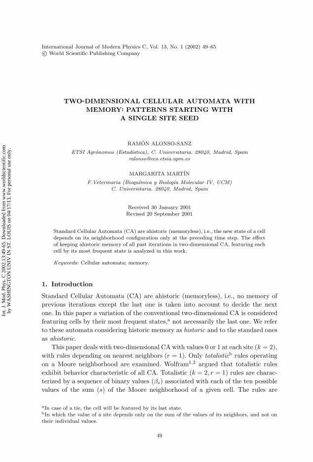
Rule 1022 (1111111110) assigns a live state to any cell whose neighborhood wouldhave at least one live cell. In the ahistoric model, a single site live cell would growas fast as it can (i.e., at the speed of light) generating squares of live cells with theirsize side increasing two units in every time step. Things happen much more slowlyin the historic model (see Table 1): the outer live cells, the perimeter of every squareof live cells, are not featured as live cells until the number of times they “live” is

Table 1. Rule 1022 (1111111110) starting with a single site live cell tillT = 16. Historic model. Live cells: last, most frequent.In

t. J.

Mod

. Phy

s. C

200

2.13

:49-

65. D

ownl

oade

d fr

om w

ww

.wor

ldsc

ient

ific

.com

by W

ASH

ING

TO

N U

NIV

IN

ST

. LO

UIS

on

04/1

7/13

. For

per

sona

l use

onl

y.


Two-Dimensional Cellular Automata with Memory 51

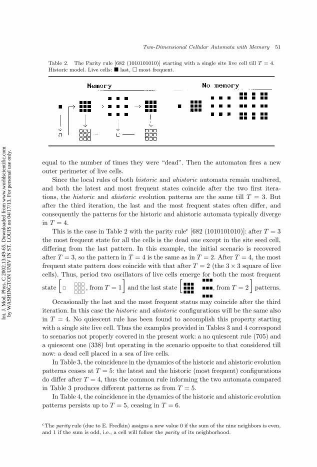
Table 2. The Parity rule [682 (1010101010)] starting with a single site live cell till T = 4.Historic model. Live cells: last, most frequent.

equal to the number of times they were “dead”. Then the automaton fires a newouter perimeter of live cells.

Since the local rules of both historic and ahistoric automata remain unaltered,and both the latest and most frequent states coincide after the two first itera-tions, the historic and ahistoric evolution patterns are the same till T = 3. Butafter the third iteration, the last and the most frequent states often differ, andconsequently the patterns for the historic and ahistoric automata typically divergein T = 4.

This is the case in Table 2 with the parity rulec [682 (1010101010)]: after T = 3the most frequent state for all the cells is the dead one except in the site seed cell,differing from the last pattern. In this example, the initial scenario is recoveredafter T = 3, so the pattern in T = 4 is the same as in T = 2. After T = 4, the mostfrequent state pattern does coincide with that after T = 2 (the 3× 3 square of livecells). Thus, period two oscillators of live cells emerge for both the most frequent

state [

, from T = 1] and the last state [

, from T = 2 ] patterns.

Occasionally the last and the most frequent status may coincide after the thirditeration. In this case the historic and ahistoric configurations will be the same alsoin T = 4. No quiescent rule has been found to accomplish this property startingwith a single site live cell. Thus the examples provided in Tables 3 and 4 correspondto scenarios not properly covered in the present work: a no quiescent rule (705) anda quiescent one (338) but operating in the scenario opposite to that considered tillnow: a dead cell placed in a sea of live cells.

In Table 3, the coincidence in the dynamics of the historic and ahistoric evolutionpatterns ceases at T = 5: the latest and the historic (most frequent) configurationsdo differ after T = 4, thus the common rule informing the two automata comparedin Table 3 produces different patterns as from T = 5.

In Table 4, the coincidence in the dynamics of the historic and ahistoric evolutionpatterns persists up to T = 5, ceasing in T = 6.

cThe parity rule (due to E. Fredkin) assigns a new value 0 if the sum of the nine neighbors is even,and 1 if the sum is odd, i.e., a cell will follow the parity of its neighborhood.

Int.

J. M

od. P

hys.

C 2

002.

13:4

9-65

. Dow

nloa

ded

from

ww

w.w

orld

scie

ntif

ic.c

omby

WA

SHIN

GT

ON

UN

IV I

N S

T. L

OU

IS o

n 04

/17/

13. F

or p

erso

nal u

se o

nly.



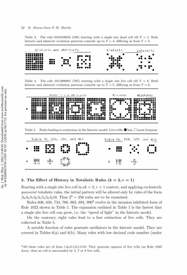
Table 3. The rule 0101010010 (338) starting with a single site dead cell till T = 5. Bothhistoric and ahistoric evolution patterns coincide up to T = 4, differing as from T = 5.

Table 4. The rule 1011000001 (705) starting with a single site live cell till T = 6. Bothhistoric and ahistoric evolution patterns coincide up to T = 5, differing as from T = 6.

Table 5. Rules leading to extinction in the historic model. Live cells: last,most frequent.

3. The Effect of History in Totalistic Rules (k = 2, r = 1)

Starting with a single site live cell in ak = 2, r = 1 context, and applying exclusivelyquiescent totalistic rules, the initial pattern will be altered only by rules of the formβ9β8β7β6β5β4β3β210. Thus 28 = 256 rules are to be examined.

Rules 606, 638, 734, 766, 862, 894, 990d evolve in the invasion inhibited form ofRule 1022 shown in Table 1. The expansion outlined in Table 1 is the fastest thata single site live cell can grow, i.e. the “speed of light” in the historic model.

On the contrary, eight rules lead to a fast extinction of live cells. They arecollected in Table 5.

A notable fraction of rules generate oscillators in the historic model. They arecovered in Tables 6(a) and 6(b). Many rules with low decimal code number (under

dAll these rules are of form 1β8β71β511110. They generate squares of live cells (as Rule 1022does), thus no cell is surrounded by 5, 7 or 8 live cells.

Int.

J. M

od. P

hys.

C 2

002.

13:4

9-65

. Dow

nloa

ded

from

ww

w.w

orld

scie

ntif

ic.c

omby

WA

SHIN

GT

ON

UN

IV I

N S

T. L

OU

IS o

n 04

/17/

13. F

or p

erso

nal u

se o

nly.



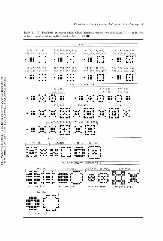
Table 6. (a) Totalistic quiescent rules, which generate period-two oscillators (` − a) in thehistoric model starting with a single site live cell ().

Int.

J. M

od. P

hys.

C 2

002.

13:4

9-65

. Dow

nloa

ded

from

ww

w.w

orld

scie

ntif

ic.c

omby

WA

SHIN

GT

ON

UN

IV I

N S

T. L

OU

IS o

n 04

/17/

13. F

or p

erso

nal u

se o

nly.



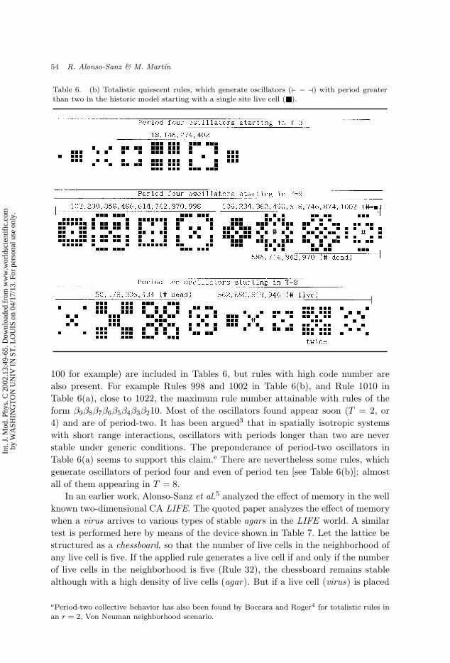
Table 6. (b) Totalistic quiescent rules, which generate oscillators (` − a) with period greaterthan two in the historic model starting with a single site live cell ().

100 for example) are included in Tables 6, but rules with high code number arealso present. For example Rules 998 and 1002 in Table 6(b), and Rule 1010 inTable 6(a), close to 1022, the maximum rule number attainable with rules of theform β9β8β7β6β5β4β3β210. Most of the oscillators found appear soon (T = 2, or4) and are of period-two. It has been argued3 that in spatially isotropic systemswith short range interactions, oscillators with periods longer than two are neverstable under generic conditions. The preponderance of period-two oscillators inTable 6(a) seems to support this claim.e There are nevertheless some rules, whichgenerate oscillators of period four and even of period ten [see Table 6(b)]; almostall of them appearing in T = 8.

In an earlier work, Alonso-Sanz et al.5 analyzed the effect of memory in the wellknown two-dimensional CA LIFE. The quoted paper analyzes the effect of memorywhen a virus arrives to various types of stable agars in the LIFE world. A similartest is performed here by means of the device shown in Table 7. Let the lattice bestructured as a chessboard, so that the number of live cells in the neighborhood ofany live cell is five. If the applied rule generates a live cell if and only if the numberof live cells in the neighborhood is five (Rule 32), the chessboard remains stablealthough with a high density of live cells (agar). But if a live cell (virus) is placed

ePeriod-two collective behavior has also been found by Boccara and Roger4 for totalistic rules inan r = 2, Von Neuman neighborhood scenario.

Int.

J. M

od. P

hys.

C 2

002.

13:4

9-65

. Dow

nloa

ded

from

ww

w.w

orld

scie

ntif

ic.c

omby

WA

SHIN

GT

ON

UN

IV I

N S

T. L

OU

IS o

n 04

/17/

13. F

or p

erso

nal u

se o

nly.



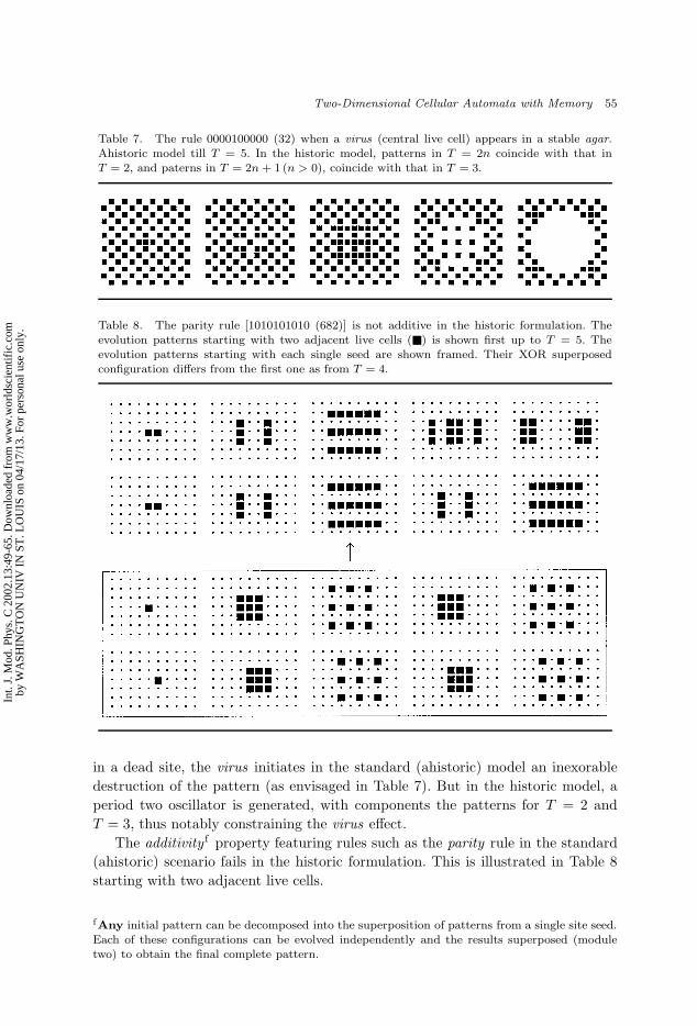
Table 7. The rule 0000100000 (32) when a virus (central live cell) appears in a stable agar.Ahistoric model till T = 5. In the historic model, patterns in T = 2n coincide with that inT = 2, and paterns in T = 2n+ 1 (n > 0), coincide with that in T = 3.

Table 8. The parity rule [1010101010 (682)] is not additive in the historic formulation. Theevolution patterns starting with two adjacent live cells () is shown first up to T = 5. Theevolution patterns starting with each single seed are shown framed. Their XOR superposedconfiguration differs from the first one as from T = 4.

in a dead site, the virus initiates in the standard (ahistoric) model an inexorabledestruction of the pattern (as envisaged in Table 7). But in the historic model, aperiod two oscillator is generated, with components the patterns for T = 2 andT = 3, thus notably constraining the virus effect.

The additivity f property featuring rules such as the parity rule in the standard(ahistoric) scenario fails in the historic formulation. This is illustrated in Table 8starting with two adjacent live cells.

fAny initial pattern can be decomposed into the superposition of patterns from a single site seed.Each of these configurations can be evolved independently and the results superposed (moduletwo) to obtain the final complete pattern.

Int.

J. M

od. P

hys.

C 2

002.

13:4

9-65

. Dow

nloa

ded

from

ww

w.w

orld

scie

ntif

ic.c

omby

WA

SHIN

GT

ON

UN

IV I

N S

T. L

OU

IS o

n 04

/17/

13. F

or p

erso

nal u

se o

nly.



4. Discounting

This section studies the effect of applying a geometric discounting process in whichthe status a obtained τ time steps before the last round is actualized to the value:ατa (α being the memory factor). A given cell will be featured by the roundedweighted mean of all its past states. This well known mechanism fully ponders thelast round (α0 = 1), and tends to forget the older rounds.

Provided that states a are coded as 0 (dead) and 1 (live), after the iteration T ,the weighted mean of the states of a given cell will be:

δ(a1, a2, . . . , aT ) =∑Ti=1 α

T−iai∑Ti=1 α

T−i.

The most frequent state (f) will be obtained comparing its weighted mean to0.5, so that:

fT =

1 if m > 0.5

aT if m = 0.5

0 if m < 0.5

.

This is equivalent to studying the sign of g:

∂(a1, a2, . . . , aT ) = 2T∑i=1

αT−iai −T∑i=1

αT−i =T∑i=1

(2ai − 1)αT−i ,

fT =

1 if ∂ > 0

aT if ∂ = 0

0 if ∂ < 0

.

After T = 3:

∂(a1, a2, a3) = α2(2a1 − 1) + α(2a2 − 1) + 2a3 − 1 .

Of course, whether a1 = a2 = a3 = 1 or a1 = a2 = a3 = 0, history does notalter the series and will be f3 = 1 and f3 = 0, respectively.h This is the case ofthe live seed cell in Tables 1 and 2. Neither does history take effect till T = 3 ifa2 = a3,i nor if a1 = a3.j Thus, in Table 1, the cells surrounding the seed, live inT = 2 and T = 3 but dead in T = 1, are featured as alive. But the scenario maychange if a1 = a2 6= a3:

∂(0, 0, 1) = −∂(1, 1, 0) = −α2 − α+ 1⇒ ∂ = 0⇔ α =−1 +

√5

2= 0.61805 .

gComputationally it is a saving if instead of calculating ∂ for every cell, we calculate ω =∑Ti=1 α

T−iai all across the lattice and compare the ω figures to the factor Ω = (1/2)∑Ti=1 α

T−i =(1/2)(αT − 1)/(α − 1).h∂(1, 1, 1) = −∂(0, 0, 0) = α2 + α+ 1 > 0.i∂(0, 1, 1) = −∂(1, 0, 0) = −α2 + α+ 1 ≥ 1 as α ≥ α2.j∂(1, 0, 1) = −∂(0, 1, 0) = α2 − α+ 1 ≥ 0.75 as max(α− α2) = 0.25 for α = 0.5.

Int.

J. M

od. P

hys.

C 2

002.

13:4

9-65

. Dow

nloa

ded

from

ww

w.w

orld

scie

ntif

ic.c

omby

WA

SHIN

GT

ON

UN

IV I

N S

T. L

OU

IS o

n 04

/17/

13. F

or p

erso

nal u

se o

nly.



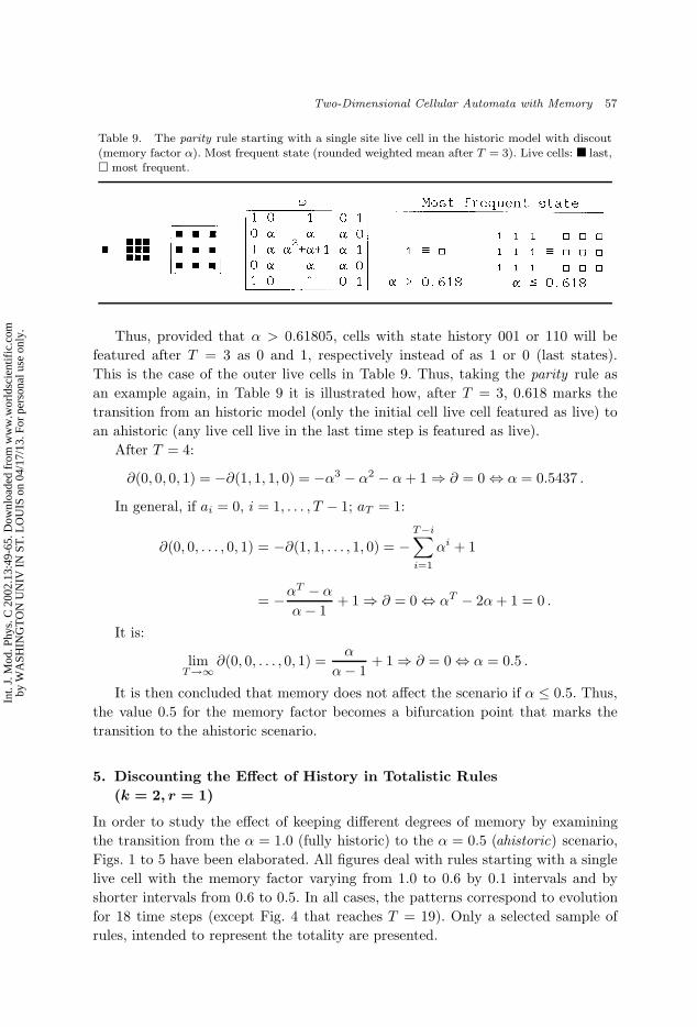
Table 9. The parity rule starting with a single site live cell in the historic model with discout

(memory factor α). Most frequent state (rounded weighted mean after T = 3). Live cells: last, most frequent.

Thus, provided that α > 0.61805, cells with state history 001 or 110 will befeatured after T = 3 as 0 and 1, respectively instead of as 1 or 0 (last states).This is the case of the outer live cells in Table 9. Thus, taking the parity rule asan example again, in Table 9 it is illustrated how, after T = 3, 0.618 marks thetransition from an historic model (only the initial cell live cell featured as live) toan ahistoric (any live cell live in the last time step is featured as live).

After T = 4:

∂(0, 0, 0, 1) = −∂(1, 1, 1, 0) = −α3 − α2 − α+ 1⇒ ∂ = 0⇔ α = 0.5437 .

In general, if ai = 0, i = 1, . . . , T − 1; aT = 1:

∂(0, 0, . . . , 0, 1) = −∂(1, 1, . . . , 1, 0) = −T−i∑i=1

αi + 1

= −αT − αα− 1

+ 1⇒ ∂ = 0⇔ αT − 2α+ 1 = 0 .

It is:

limT→∞

∂(0, 0, . . . , 0, 1) =α

α− 1+ 1⇒ ∂ = 0⇔ α = 0.5 .

It is then concluded that memory does not affect the scenario if α ≤ 0.5. Thus,the value 0.5 for the memory factor becomes a bifurcation point that marks thetransition to the ahistoric scenario.

5. Discounting the Effect of History in Totalistic Rules(k = 2, r = 1)

In order to study the effect of keeping different degrees of memory by examiningthe transition from the α = 1.0 (fully historic) to the α = 0.5 (ahistoric) scenario,Figs. 1 to 5 have been elaborated. All figures deal with rules starting with a singlelive cell with the memory factor varying from 1.0 to 0.6 by 0.1 intervals and byshorter intervals from 0.6 to 0.5. In all cases, the patterns correspond to evolutionfor 18 time steps (except Fig. 4 that reaches T = 19). Only a selected sample ofrules, intended to represent the totality are presented.

Int.

J. M

od. P

hys.

C 2

002.

13:4

9-65

. Dow

nloa

ded

from

ww

w.w

orld

scie

ntif

ic.c

omby

WA

SHIN

GT

ON

UN

IV I

N S

T. L

OU

IS o

n 04

/17/

13. F

or p

erso

nal u

se o

nly.



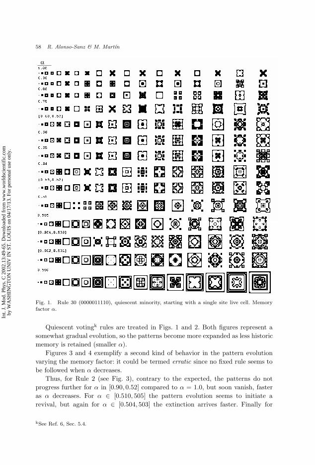
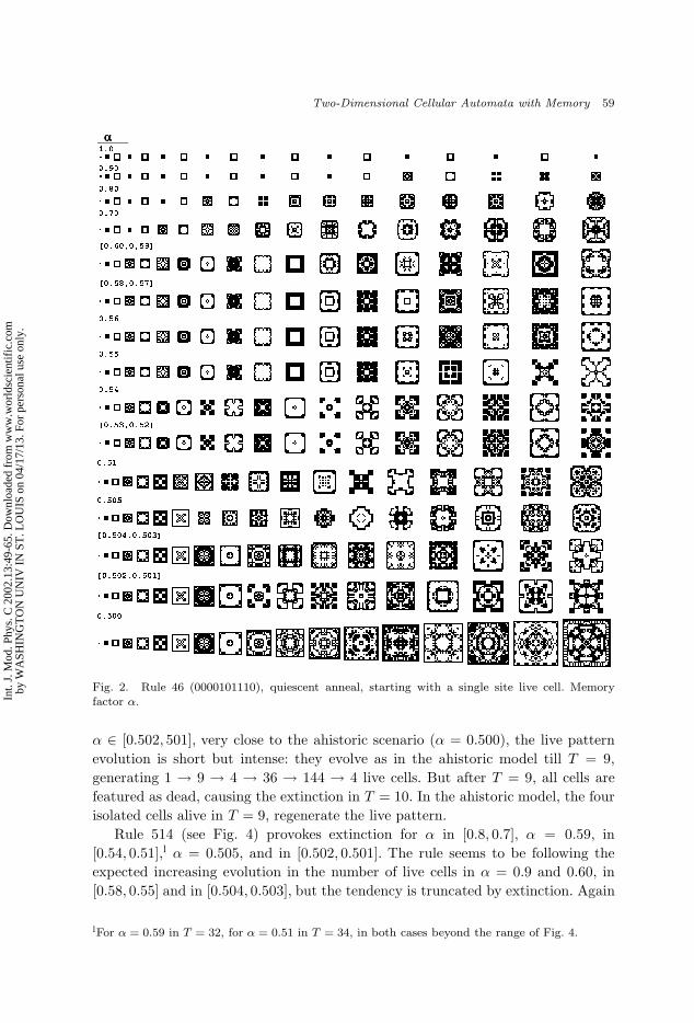
Fig. 1. Rule 30 (0000011110), quiescent minority, starting with a single site live cell. Memoryfactor α.

Quiescent votingk rules are treated in Figs. 1 and 2. Both figures represent asomewhat gradual evolution, so the patterns become more expanded as less historicmemory is retained (smaller α).

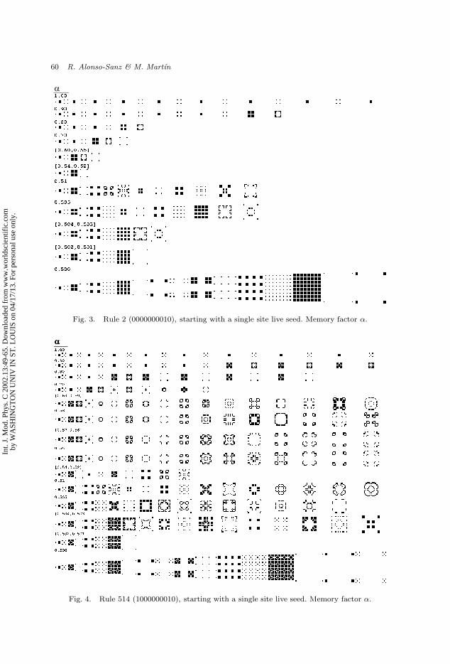
Figures 3 and 4 exemplify a second kind of behavior in the pattern evolutionvarying the memory factor: it could be termed erratic since no fixed rule seems tobe followed when α decreases.

Thus, for Rule 2 (see Fig. 3), contrary to the expected, the patterns do notprogress further for α in [0.90, 0.52] compared to α = 1.0, but soon vanish, fasteras α decreases. For α ∈ [0.510, 505] the pattern evolution seems to initiate arevival, but again for α ∈ [0.504, 503] the extinction arrives faster. Finally for

kSee Ref. 6, Sec. 5.4.

Int.

J. M

od. P

hys.

C 2

002.

13:4

9-65

. Dow

nloa

ded

from

ww

w.w

orld

scie

ntif

ic.c

omby

WA

SHIN

GT

ON

UN

IV I

N S

T. L

OU

IS o

n 04

/17/

13. F

or p

erso

nal u

se o

nly.



Fig. 2. Rule 46 (0000101110), quiescent anneal, starting with a single site live cell. Memoryfactor α.

α ∈ [0.502, 501], very close to the ahistoric scenario (α = 0.500), the live patternevolution is short but intense: they evolve as in the ahistoric model till T = 9,generating 1 → 9 → 4 → 36 → 144 → 4 live cells. But after T = 9, all cells arefeatured as dead, causing the extinction in T = 10. In the ahistoric model, the fourisolated cells alive in T = 9, regenerate the live pattern.

Rule 514 (see Fig. 4) provokes extinction for α in [0.8, 0.7], α = 0.59, in[0.54, 0.51],l α = 0.505, and in [0.502, 0.501]. The rule seems to be following theexpected increasing evolution in the number of live cells in α = 0.9 and 0.60, in[0.58, 0.55] and in [0.504, 0.503], but the tendency is truncated by extinction. Again

lFor α = 0.59 in T = 32, for α = 0.51 in T = 34, in both cases beyond the range of Fig. 4.

Int.

J. M

od. P

hys.

C 2

002.

13:4

9-65

. Dow

nloa

ded

from

ww

w.w

orld

scie

ntif

ic.c

omby

WA

SHIN

GT

ON

UN

IV I

N S

T. L

OU

IS o

n 04

/17/

13. F

or p

erso

nal u

se o

nly.



Fig. 3. Rule 2 (0000000010), starting with a single site live seed. Memory factor α.

Fig. 4. Rule 514 (1000000010), starting with a single site live seed. Memory factor α.

Int.

J. M

od. P

hys.

C 2

002.

13:4

9-65

. Dow

nloa

ded

from

ww

w.w

orld

scie

ntif

ic.c

omby

WA

SHIN

GT

ON

UN

IV I

N S

T. L

OU

IS o

n 04

/17/

13. F

or p

erso

nal u

se o

nly.



close to the ahistoric scenario (0.502 ≤ α ≤ 501), a peak of 148 live cells in T = 8is followed by only four in T = 9 (as in the ahistoric scenario) and by extinction inT = 10.

The erratic kind of behavior has been found to affect only rules that generateoscillators in the fully historic model, such as Rules 2 and 514.

All the rules that generate the same period-two oscillator as Rule 2 (see Table 5)behave erratically: Rules 130, 258 and 386 exactly as Rule 2; for Rules 34 and 290extinction is found for α in [0.9, 0.6], [0.54, 0.52] and [0.502, 0.501]; Rules 162 and418 provoke extinction for the same α values as 34 and 29 except for α = 0.7.

Rule 642 evolves as 514 (except with no extinction in α = 0.51], Rule 770 inducesextinction for α = 0.7, α = 0.59 and in [0.54, 0.52); Rule 898 only for α = 0.7 andα = 0.59. Rules 546, 674, 802 and 930 do not evolve erratically.

The other rules that generate period-two oscillators in the fully historic modeland behave erratically to some extent (at least with one unexpected extinction)are: Rules 6, 38, 134, 166, 262, 294, 390, 422; 10, 42, 138, 170, 266, 394; 82, 210;198, 454; 530, 658, 786, 914; 70 and 326.

Rules 18, 146, 274 and 402 are the only rules generating period four oscillatorsin the fully historic model that lead to extinction for some memory factor values(0.7, [0.9, 0.7], 0.7 and 0.9, respectively).

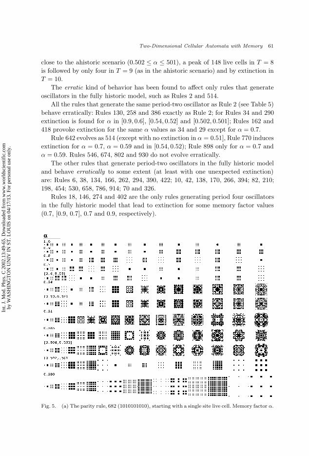
Fig. 5. (a) The parity rule, 682 (1010101010), starting with a single site live cell. Memory factor α.

Int.

J. M

od. P

hys.

C 2

002.

13:4

9-65

. Dow

nloa

ded

from

ww

w.w

orld

scie

ntif

ic.c

omby

WA

SHIN

GT

ON

UN

IV I

N S

T. L

OU

IS o

n 04

/17/

13. F

or p

erso

nal u

se o

nly.



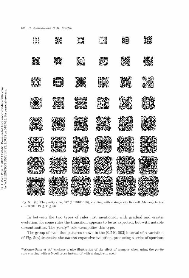
Fig. 5. (b) The parity rule, 682 (1010101010), starting with a single site live cell. Memory factorα = 0.501. 19 ≤ T ≤ 56.

In between the two types of rules just mentioned, with gradual and erraticevolution, for some rules the transition appears to be as expected, but with notablediscontinuities. The paritym rule exemplifies this type.

The group of evolution patterns shown in the (0.540, 503] interval of α variationof Fig. 5(a) truncates the natural expansive evolution, producing a series of spurious

mAlonso-Sanz et al.5 encloses a nice illustration of the effect of memory when using the parityrule starting with a 5-cell cross instead of with a single-site seed.

Int.

J. M

od. P

hys.

C 2

002.

13:4

9-65

. Dow

nloa

ded

from

ww

w.w

orld

scie

ntif

ic.c

omby

WA

SHIN

GT

ON

UN

IV I

N S

T. L

OU

IS o

n 04

/17/

13. F

or p

erso

nal u

se o

nly.



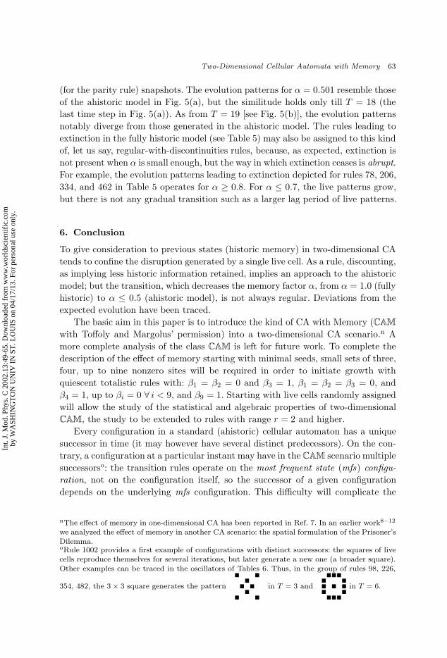
(for the parity rule) snapshots. The evolution patterns for α = 0.501 resemble thoseof the ahistoric model in Fig. 5(a), but the similitude holds only till T = 18 (thelast time step in Fig. 5(a)). As from T = 19 [see Fig. 5(b)], the evolution patternsnotably diverge from those generated in the ahistoric model. The rules leading toextinction in the fully historic model (see Table 5) may also be assigned to this kindof, let us say, regular-with-discontinuities rules, because, as expected, extinction isnot present when α is small enough, but the way in which extinction ceases is abrupt.For example, the evolution patterns leading to extinction depicted for rules 78, 206,334, and 462 in Table 5 operates for α ≥ 0.8. For α ≤ 0.7, the live patterns grow,but there is not any gradual transition such as a larger lag period of live patterns.

6. Conclusion

To give consideration to previous states (historic memory) in two-dimensional CAtends to confine the disruption generated by a single live cell. As a rule, discounting,as implying less historic information retained, implies an approach to the ahistoricmodel; but the transition, which decreases the memory factor α, from α = 1.0 (fullyhistoric) to α ≤ 0.5 (ahistoric model), is not always regular. Deviations from theexpected evolution have been traced.

The basic aim in this paper is to introduce the kind of CA with Memory (CAMwith Toffoly and Margolus’ permission) into a two-dimensional CA scenario.n Amore complete analysis of the class CAM is left for future work. To complete thedescription of the effect of memory starting with minimal seeds, small sets of three,four, up to nine nonzero sites will be required in order to initiate growth withquiescent totalistic rules with: β1 = β2 = 0 and β3 = 1, β1 = β2 = β3 = 0, andβ4 = 1, up to βi = 0 ∀ i < 9, and β9 = 1. Starting with live cells randomly assignedwill allow the study of the statistical and algebraic properties of two-dimensionalCAM, the study to be extended to rules with range r = 2 and higher.

Every configuration in a standard (ahistoric) cellular automaton has a uniquesuccessor in time (it may however have several distinct predecessors). On the con-trary, a configuration at a particular instant may have in the CAM scenario multiplesuccessorso: the transition rules operate on the most frequent state (mfs) configu-ration, not on the configuration itself, so the successor of a given configurationdepends on the underlying mfs configuration. This difficulty will complicate the

nThe effect of memory in one-dimensional CA has been reported in Ref. 7. In an earlier work8–12

we analyzed the effect of memory in another CA scenario: the spatial formulation of the Prisoner’sDilemma.oRule 1002 provides a first example of configurations with distinct successors: the squares of livecells reproduce themselves for several iterations, but later generate a new one (a broader square).Other examples can be traced in the oscillators of Tables 6. Thus, in the group of rules 98, 226,

354, 482, the 3× 3 square generates the pattern

in T = 3 and

in T = 6.

Int.

J. M

od. P

hys.

C 2

002.

13:4

9-65

. Dow

nloa

ded

from

ww

w.w

orld

scie

ntif

ic.c

omby

WA

SHIN

GT

ON

UN

IV I

N S

T. L

OU

IS o

n 04

/17/

13. F

or p

erso

nal u

se o

nly.



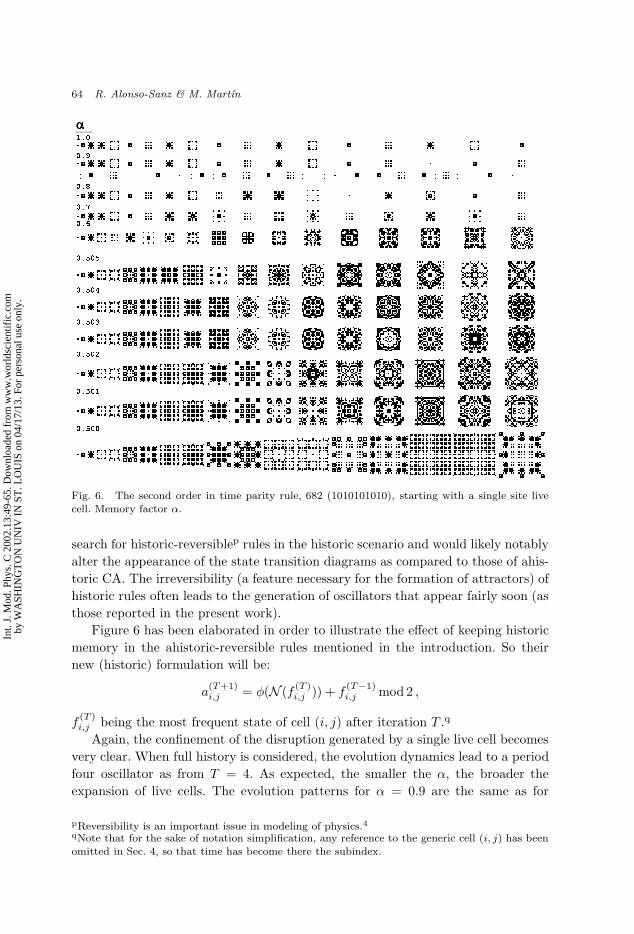
Fig. 6. The second order in time parity rule, 682 (1010101010), starting with a single site livecell. Memory factor α.

search for historic-reversiblep rules in the historic scenario and would likely notablyalter the appearance of the state transition diagrams as compared to those of ahis-toric CA. The irreversibility (a feature necessary for the formation of attractors) ofhistoric rules often leads to the generation of oscillators that appear fairly soon (asthose reported in the present work).

Figure 6 has been elaborated in order to illustrate the effect of keeping historicmemory in the ahistoric-reversible rules mentioned in the introduction. So theirnew (historic) formulation will be:

a(T+1)i,j = φ(N (f (T )

i,j )) + f(T−1)i,j mod 2 ,

f(T )i,j being the most frequent state of cell (i, j) after iteration T .q

Again, the confinement of the disruption generated by a single live cell becomesvery clear. When full history is considered, the evolution dynamics lead to a periodfour oscillator as from T = 4. As expected, the smaller the α, the broader theexpansion of live cells. The evolution patterns for α = 0.9 are the same as for

pReversibility is an important issue in modeling of physics.4qNote that for the sake of notation simplification, any reference to the generic cell (i, j) has beenomitted in Sec. 4, so that time has become there the subindex.

Int.

J. M

od. P

hys.

C 2

002.

13:4

9-65

. Dow

nloa

ded

from

ww

w.w

orld

scie

ntif

ic.c

omby

WA

SHIN

GT

ON

UN

IV I

N S

T. L

OU

IS o

n 04

/17/

13. F

or p

erso

nal u

se o

nly.



α = 1.0 up to T = 15, but in T = 16, unlike those in the fully historic model,only the initial live cell is alive. In T = 21, no cell is alive; but this does not meanextinction: in T = 22, eight cells are alive. This odd cataleptic phenomenon is fairlyfrequent in the α = 0.9 context of Fig. 6, which shows two more cases of it.

Acknowledgment

Computing was performed using the computing facilities of the Department ofMathematics and Statistics, University of Edinburgh. Dr. M. Ibanez-Ruiz (ETSIAgronomos (Estadıstica)) has contributed to the computer implementation of thiswork.

References

1. S. Wolfram, Physica D 10, 1 (1984).2. S. Wolfram, J. Stat. Phys. 38, 901 (1985).3. G. Grinstein, J. Stat. Phys. A 5, 803 (1988).4. N. Margolus, Physica D 10, 81 (1984).5. R. Alonso-Sanz, M. C. Martin, and M. Martin, Int. J. Bifurcation and Chaos 11, 1665

(2001).6. T. Toffoli and N. Margolus, Cellular Automata Machines (MIT Press, 1987).7. R. Alonso-Sanz and M. Martin, Int. J. Bifurcation and Chaos 12 (2002).8. R. Alonso-Sanz, Int. J. Bifurcation and Chaos 9, 1197 (1999).9. R. Alonso-Sanz, M. C. Martin, and M. Martin, Int. J. Bifurcation and Chaos 10, 87

(2000).10. R. Alonso-Sanz, M. C. Martin, and M. Martin, Int. J. Bifurcation and Chaos 11, 943

(2001).11. R. Alonso-Sanz, M. C. Martin, and M. Martin, Int. J. Bifurcation and Chaos 11, 2037

(2001).12. R. Alonso-Sanz, M. C. Martin, and M. Martin, Int. J. Bifurcation and Chaos 11

(2001).13. N. Boccara and M. Roger, Int. J. Mod. Phys. C 10, 1 (1999).

Int.

J. M

od. P

hys.

C 2

002.

13:4

9-65

. Dow

nloa

ded

from

ww

w.w

orld

scie

ntif

ic.c

omby

WA

SHIN

GT

ON

UN

IV I

N S

T. L

OU

IS o

n 04

/17/

13. F

or p

erso

nal u

se o

nly.

Documents

TWO-DIMENSIONAL CELLULAR AUTOMATA WITH MEMORY: PATTERNS STARTING WITH A SINGLE SITE SEED