arX

iv:1

608.

0016

0v1

[m

ath.

AP]

30

Jul 2

016

Twists and shear maps in nonlinear

elasticity: explicit solutions and vanishing

Jacobians

Jonathan J. Bevan∗ and Sandra Kabisch∗

August 2, 2016

Abstract

In this paper we study constrained variational problems that are principally mo-tivated by nonlinear elasticity theory. We examine in particular the relationshipbetween the positivity of the Jacobian det∇u and the uniqueness and regularityof energy minimizers u that are either twist maps or shear maps. We exhibit ex-plicit twist maps, defined on two-dimensional annuli, that are stationary points ofan appropriate energy functional and whose Jacobian vanishes on a set of positivemeasure in the annulus. Within the class of shear maps we precisely characterize theunique global energy minimizer uσ : Ω → R

2 in a model, two-dimensional case. Theshear map minimizer has the properties that (i) det∇uσ is strictly positive on onepart of the domain Ω, (ii) det∇uσ = 0 necessarily holds on the rest of Ω, and (iii)properties (i) and (ii) combine to ensure that ∇uσ is not continuous on the wholedomain.

1 Introduction

In this paper we consider minimizers of variational problems that are motivated bynonlinear elasticity theory. The functionals we wish to minimize are of the form

I(u) =

ˆ

ΩW (∇u(x)) dx,

where Ω ⊂ R2 is a domain representing the reference configuration of an elastic material,

W : R2×2 → [0,+∞] its stored energy function and u : Ω → R2 a deformation. One

of the tenets of the theory is that the noninterpenetrability of matter is encoded byrequiring that det∇u > 0 a.e.in Ω. This is typically imposed by setting W (F ) = +∞whenever the 2 × 2 matrix F satisfies detF ≤ 0, so that any deformation having finiteenergy necesssarily satisfies det∇u > 0 a.e. The main purpose of this paper is to

∗Department of Mathematics, University of Surrey, Guildford, UK. e: j.bevan@surrey.ac.uk

1

examine in particular the relationship between the positivity of the Jacobian det∇u andthe uniqueness and regularity of two different kinds of stationary point associated withthe energy functional I(·).

The first kind of stationarity results in the so-called Energy-Momentum (EM) equa-tions

div (∇uTDW (∇u)−W (∇u)1) = 0 (1)

formally obtained from I(·) by setting ∂ǫ|ǫ=0I(uǫ) = 0 in the case that uǫ(x) = u(x +

ǫϕ(x)) and ϕ is a smooth, compactly supported test function. Conditions guaranteeingthat (1) holds in a rigorous sense can be found in [1, 2]. The second type of stationarityresults formally in the Euler-Lagrange (EL) equations,

divDW (∇u) = 0, (2)

whose derivation from ∂ǫ|ǫ=0I(u+ ǫϕ) = 0, when the latter exists, is well known.The sorts of stationary point we consider fall into two broad classes: twists and shears.

Twist maps operate on an annulus A = x ∈ R2 : a < |x| < b and act as the identity

on ∂A. Shear maps are of the form u(x) = x + σ(x)e, where e is a fixed unit vectorand σ a scalar field defined on some domain, which in this paper will typically be asquare Q := [−1, 1]2. We study two types of functional in each of the twist and shearmap classes: both are of the form I(u) =

´

ΩW (∇u(x)) dx where the set Ω is either theannulus, A, or the square, Q, and W is of the form

W (F ) =1

2|F |2 + h(detF ) (3)

defined on 2 × 2 matrices F . The function h is either (i) of the kind that penalizesdetF → 0 in the sense that h = h0 and h0(s) → +∞ as s → 0+, h0(s) = +∞ for s ≤ 0and h0 is convex where it is finite1, or (ii) of the form

h∞(s) =

0 if s ≥ 0+∞ if s < 0.

Type (i) functions h0 penalize compression to zero area, while type (ii) functions h∞ensure that maps u with finite energy obey det∇u ≥ 0 almost everywhere in Ω.

Thus there are effectively four permutations, and together they generate the range ofbehaviours summarised in the table below.

1See Section 2.2 for details of additional hypotheses imposed on h0

2

W (F ) = 12 |F |

2 + h0(detF ) W (F ) = 12 |F |

2 + h∞(detF )

TwistMaps

• infinitely many solutions of (EL)(see [13])• Jacobian bounded away from 0 onA• solutions belong to the class C3(A)(see [13])

• infinitely many solutions of (EM)• Jacobian vanishes on set of positivemeasure• solutions are explicit and of classC1(A)

ShearMaps

• solution of (EL) unique 2

• Singularities at boundary canform 3

• solution of (EL) unique• Jacobian vanishes on set of positivemeasure• solution cannot be of class C1(Q) forappropriate boundary data

The non-uniqueness of solutions to the Euler-Lagrange equations of elasticity problemswith mixed boundary conditions is a well known phenomenon, such as in the buckling of arod or beam. However, for pure displacement boundary conditions things are not so clear.Indeed, it is still an open question whether sufficiently smooth equilibrium solutionsto pure displacement boundary-value problems for homogeneous bodies with strictlypolyconvex stored energy function W are unique if the domain Ω is homeomorphicto a ball (see Problem 8, [2]). Much work has been done in this area: see [14, 6,15, 11, 16] and [10]. F. John showed in [10] that a twice continuously differentiableequilibrium of sufficiently small strain is unique. In the same paper, the author formallysuggested that multiple solutions to the Euler-Lagrange equations might be found amongthe twist maps of a two-dimensional annulus (cf. Problem 8, [2]). Solutions of thiskind were subsequently found by Post and Sivaloganathan4 in [13] in the case thath = h0, in the notation introduced above, and led to Francfort and Sivaloganathan’sexploration of the case h = h∞ in [7]. When h = h0, our contribution is to improve theregularity of the twist maps they found and to deduce that the Jacobian of each solutionof the Euler-Lagrange equations is bounded away from zero, in contrast to the situationencountered when compression to zero area is not penalized, that is when h = h∞. Thisis done by using techniques of Baumann, Owen and Phillips [4, 5] to show that auxiliaryfunctions d = det∇u and z = 1

2 |∇u|2 + f(det∇u), where f(d) = h′0(d)d − h0(d), are,

respectively, monotonically increasing and decreasing along the radius of the annulus. Asan additional property, we also present a maximum principle for the function ρ

r:= |u(x)|

|x| ,

where r = |x|. It remains an open question whether the global energy minimizers in thiscase are necessarily rotationally symmetric.

4These authors also extended their arguments to the torus in 3 dimensions.

3

In the case that h = h∞, we obtain infinitely many explicit5 rotationally symmetricsolutions to the Energy-Momentum equations, which are parametrized by the numberof times N , say, that the outer boundary Sb := x ∈ R

2 : |x| = b of the annulus A istwisted around the inner boundary Sa (using similar notation). All these solutions sharethe property that an annular region x ∈ R

2 : a ≤ |x| ≤ k around the inner boundarySa of A is mapped onto Sa, thereby compressing that region to ‘zero area’. This region,which we call the ‘hedgehog region’ for reasons explained later in the paper, is wheremost of the twisting happens: at most one quarter of the twist is performed outside thehedgehog region, regardless of the size of N . See Section 2.2 for details. It is interestingto note that our explicit solutions do not solve the Euler-Lagrange equations6, the proofof which relies on an observation of [7]. We also show that our equilibrium solutionsare local minimizers in suitably restricted classes of twist maps: see Proposition 6 andCorollary 7.

In the context of shear maps, the results of Section 3 focus on the relationship betweenthe regularity of global energy minimizers and the positivity of the Jacobian, among otherthings. Minimizing shear maps uσ are unique because the map σ 7→ I(uσ) is strictlyconvex as a functional and, as is explained in Section 3, the class of admissible functionsis convex as a set. The former is obvious when h = h∞ and surprising when h = h0:see Lemma 18 for details. Using the same notation as above, we find a condition thatcharacterizes the shear map minimizer of I∞ and which, in conjunction with a carefullychosen type of boundary condition, provides conditions under which the global shearmap minimizer, uσ,∞, say, is not of class C1. The boundary condition, which can easilybe generalized, ensures that det∇uσ,∞ = 0 on a set of positive measure in Q, somethingit has in common with the twist solutions of Section 2.1.

In the final part of the paper we prove that, under certain mixed boundary condi-tions, which again can be generalized, the shear map minimizer uσ,0, say, of I0 is suchthat ∇uσ,0 is not continuous at the ‘corners’ of Q. This happens under the additionalassumption that det∇uσ,0 ≥ c > 0 a.e., which would normally be thought of as a reg-ularizing condition, but which here seems to focus discontinuities in ∇uσ,0 at points on∂Q where the character of the boundary condition changes from mixed to traction-free.The analysis relies on results from elliptic regularity theory that are applicable preciselybecause σ 7→W (∇uσ) is strongly convex.

1.1 Notation

We denote the 2 × 2 real matrices by R2×2, and unless stated otherwise we sum over

repeated indices. The tensor product of two vectors a ∈ R2 and b ∈ R

2 is written a⊗ b;it is the 2 × 2 matrix whose (i, j) entry is aibj. The inner product of two matricesX,Y ∈ R

2×2 is X · Y = tr(XTY ). This obviously holds for vectors too. For pointsx = (r, θ) in plane polar coordinates and belonging to a domain Ω ⊂ R

2, the gradient of

5These examples seem to be very rare in the literature.6To be precise, these take the form of a variational inequality.

4

ϕ : Ω → R2 is

∇ϕ = ϕ,r ⊗ er(θ) +1

rϕ,θ ⊗ eτ (θ),

where er(θ) = (cos θ, sin θ)T and eτ (θ) = (− sin θ, cos θ)T . Throughout the paper wewrite ϕ,r = ∂rϕ, ϕ,θ = ∂θϕ and ϕ,τ = 1

r∂θϕ. In this notation the formula

det∇ϕ = Jϕ,r · ϕ,τ

holds, where J is the 2× 2 matrix corresponding to a rotation of π2 radians in the plane,

i.e.,

J =

(0 −11 0

).

The two most useful properties of J are that (i) JT = −J , so that in particular a · Jb =−Ja · b for any two a, b ∈ R

2, and (ii) cof A = JTAJ for any 2× 2 matrix A. We denotethe identity matrix by 1. Derivatives with respect to cartesian coordinates xi for i = 1, 2will be usually be written ϕ,xi

, and occasionally ∂xiϕ.

A function f : R2×2 → R ∪ +∞ is said to be polyconvex if there exists a convexfunction φ : R2×2 ×R → R ∪ +∞ such that

f(A) = φ(A,detA)

for all 2× 2 real matrices A. The function space setting for all the problems we considerwill be W 1,2(Ω;R2), which we will abbreviate to W 1,2(Ω) whenever it is unambiguousto do so. As usual, represents weak convergence in both the Sobolev space W 1,2(Ω)and the Lebesgue space L2(Ω). Since Ω ⊂ R

2, the appropriate notion of boundarymeasure, as generated by the boundary integrals in Green’s theorem, for example, isone-dimensional Hausdorff measure, which we write either as dH1 or, in the case of acircular boundary, dS.

Other, standard notation includes B(a, r) for the ball in R2 centred at a with radius

r and Sr for the circle centred at 0 of radius r. We write A(p, q) for the annulusB(0, q) \B(0, p), where p < q, and when it causes no confusion, we abbreviate A(a, b) toA.

2 Minimizers in the class of twist maps

We begin by recalling the technical setting of twist maps first proposed in [13]. LetA = x ∈ R

2 : a < |x| < b and set

A = u ∈W 1,2(A) : u = id on ∂A. (4)

Following [13, Section 2], one now selects subclasses of A by means of the windingnumber. Formally, for each integer N we restrict attention to maps u : A → R

2 whichrotate the outer boundary x ∈ R

2 : |x| = b N times relative to the inner boundary

5

x ∈ R2 : |x| = a. More precisely, changing to polar coordinates and applying the

ACL property of Sobolev functions, it is the case that for a.e. θ ∈ [0, 2π] the curve

γθ :=

u(r, θ)

|u(r, θ)|: a ≤ r ≤ b

is closed and continuous. The winding number for such curves is defined by approxi-mation using C1 curves in the plane. We recall that the winding number of a closedC1 curve in the plane, i.e. γ : [a, b] → R

2 with γ(a) = γ(b) and γ(r) = (x(r), y(r)), isdefined by

wind#γ =1

2π

ˆ b

a

x(r)y′(r)− x′(r)y(r)

x2(r) + y2(r)r.. (5)

For each integer N let

AN = u ∈ A : wind#γθ = N for a.e. θ ∈ [0, 2π]. (6)

By [13, Lemma 2.7] each class AN is closed with respect to weak convergence inW 1,2(A).The existence of a minimizer of I(u) =

´

AW (∇u) dx then follows easily by applying the

direct method of the calculus of variations. We will apply this procedure both in the casethat compression to zero area is penalized and when it is not, corresponding respectivelyto the choice h = h0 and h = h∞ in the stored-energy function W . We turn first to thecase h = h∞.

2.1 The case h = h∞: twist minimizers without area compression energy

The problem we consider here was raised in Francfort and Sivaloganathan [7] and is illus-trative of the case where the Euler-Lagrange equations are not satisfied by minimizers:see Remark 2 below. Using the framework of [13], our approach is to seek solutions ofthe Energy-Momentum equations for the functional

I∞(u) =

ˆ

A

1

2|∇u|2 + h∞(det∇u) dx

in the class

AN = u ∈ A : wind#γθ = N for a.e. θ ∈ [0, 2π], (7)

where the class A is given by (4). This is clearly equivalent to minimizing a Dirichletenergy

D(u) :=

ˆ

A

|∇u|2 dx (8)

on the set

AN = u ∈ A : wind#γθ = N for a.e. θ ∈ [0, 2π], (9)

where

A = u ∈W 1,2(A) : u = id on ∂A and det∇u ≥ 0 a.e. in A. (10)

6

Proposition 1. Let I∞ and AN be as above. Then there is a minimizer of I∞ in AN .

Proof. We apply the direct method of the calculus of variations to the formulation ofthe problem in terms of the Dirichlet integral D(u). Note that AN contains the map

U(x) = r

(cos

(θ + 2Nπ

(r − a

b− a

)), sin

(θ + 2Nπ

(r − a

b− a

))),

where x = r(cos θ, sin θ), so that AN is in particular nonempty. To show that it isweakly closed we appeal first to [13, Lemma 2.7] to ensure that the weak limit u, say, inW 1,2(A) of any sequence u(j) in AN obeys the winding number constraint and boundaryconditions. Moreover, from [12, Corollary 1.2], it follows that det∇u ≥ 0 a.e. in Awhen det∇u(j) ≥ 0 a.e. holds for all j and ∇u(j) ∇u in L2(A). Hence AN is weaklyclosed. A straightforward argument using the convexity of the Dirichlet energy impliesthat D(·) is sequentially weakly lower semicontinuous, from which the existence of aminimizer follows.

Remark 2. We expect that the minimizer uN of I∞ in AN for N 6= 0 to be degeneratein the sense that det∇uN cannot be bounded away from 0. This is because if thereexists c > 0 such that det∇uN ≥ c in A then the Euler-Lagrange equations for I∞ areequivalent to

∆u = 0 in A

u = id on ∂A,(11)

which, by standard theory, has the unique solution u = id, and which does not obey thewinding number condition (u = id clearly has winding number zero). One way in whichdet∇uN could fail to be a.e. bounded away from 0 is for it to vanish on a set of positivemeasure in A: this is certainly the case for the symmetric minimizers of which we givedetails later.

It is straightforward to check that the energy momentum equations associated withI∞ are, in a distributional sense,

div

(1

2|∇u|21−∇uT∇u

)= 0 in A

u = id on ∂A.

(12)

We seek a rotationally symmetric solution of this system, i.e. a solution from the set

AN, sym = u ∈ AN : u(x) = QTu(Qx) for all Q ∈ SO(2). (13)

That such a solution exists follows from the same argument used in the proof of Propo-sition 1. Rotationally symmetric solutions can be represented in polar coordinates as

u(r, θ) = ρ(r)er(θ + ψ(r)) (14)

7

where er(θ) = (cos θ, sin θ). For brevity we shall henceforth write er for er(θ) and er forer(θ + ψ(r)). Similarly, we define eθ(θ) = (− sin θ, cos θ) and use the abbreviations eθand eθ analogously. We call ρ the radial map and ψ the angular map. In this notation,we have the following result.

Lemma 3. Let N ∈ N. Then the radial map ρ of a minimizer of I∞ in AN, sym isdifferentiable and satisfies the ODE

ρ =1

r

√ρ2 −

ω2

ρ2− a2 +

ω2

a2(15)

ρ(a) = a, ρ(b) = b. (16)

for some ω ∈ (0,+∞). Furthermore, the angular map ψ is differentiable with

ψ =ω

Rρ2(17)

and ψ(a) = 0 and ψ(b) = 2πN .

Proof. To prove this we test the weak form of (12) with a rotationally symmetric testfunction φ. We can express φ as

φ(r, θ) = ρ(r)er + q(r)eθ. (18)

with ρ, q ∈ C∞c ((a, b)). Furthermore

∇u = ρer ⊗ er + ρψeθ ⊗ er +ρ

reθ ⊗ eθ, (19)

∇φ = ˙ρer ⊗ er + ˙qeθ ⊗ er +1

r[ρeθ ⊗ eθ − qer ⊗ eθ] , (20)

and

|∇u|2 = ρ2 + ρ2ψ2 +ρ2

r2. (21)

Therefore,

1

2|∇u|2I −∇uT∇u =

1

2

(ρ2 + ρ2ψ2 +

ρ2

r2

)I −

((ρ2 + ρ2ψ2)er ⊗ er

+ρ2ψ

r(er ⊗ eθ + eθ ⊗ er) +

ρ2

r2eθ ⊗ eθ

), (22)

8

so that

0 =

ˆ

A

[1

2|∇u|2I −∇uT∇u

]· ∇φdx

= 2π

ˆ b

a

r

2

(ρ2 + ρ2ψ2 +

ρ2

r2

)(˙ρ+

ρ

r

)

− r

((ρ2 + ρ2ψ2) ˙ρ+

ρ2ψ

r

(˙q −

q

r

)+ρ2

r2ρ

r

)dr

= 2π

ˆ b

a

r

2

(ρ2 + ρ2ψ2 −

ρ2

r2

)(ρ

r− ˙ρ

)+ r

ρ2ψ

r

(q

r− ˙q

)dr

= −2π

ˆ b

a

r2

2

(ρ2 + ρ2ψ2 −

ρ2

r2

)(ρ

r

)·+ rρ2ψ

(q

r

)·dr. (23)

Since ρ and q are arbitrary this implies that there exist constants c and ω s.t.

r2(ρ2 + ρ2ψ2 −

ρ2

r2

)= c in (a, b) (24)

and

rρ2ψ = ω in (a, b). (25)

Furthermore, since´

A|∇u|2 dx < ∞, it follows that ρ ∈ W 1,2((a, b)), which in turn

yields ρ ∈ C([a, b]). Therefore ψ = ωrρ2

∈ C([a, b]) as well. That ω > 0 simply follows

from the fact that, by (25), ψ is a monotonic function and we want to achieve a positivewinding number, i.e. ψ(b) = 2πN > 0 and ψ(a) = 0. Substituting ψ back into (24) weobtain

r2ρ2 +ω2

ρ2− ρ2 = c (26)

which also implies that the weak derivative ρ is continuous and is therefore the classicalderivative. Since det∇u = ρρ

r≥ 0, we find that ρ2 is monotonically increasing. Therefore

ρ ≥ a > 0 which in turn implies ρ ≥ 0. Hence we can solve for ρ in (26) to obtain (16).

Now we want to prove that c = −a2+ ω2

a2. In view of (26), this is equivalent to showing

that ρ(a) has to be zero. This is done in two steps: first we show that if ρ vanishes thenit can only do so at r = a, and then we prove that ρ(a) > 0 is impossible, which, sinceρ is nonnegative, leaves only the possibility that ρ(a) = 0.

Assume for a contradiction that there is a point r ∈ (a, b] s.t. ρ(r) = 0 and ρ(r) > 0 forr ∈ (r−δ,r) for some δ > 0, meaning that we suppose ρ has a zero at the rightmost point

of an interval where it is strictly positive. Let z(r) = f(ρ(r)) where f(ρ) = ρ2 − ω2

ρ2+ c

and note that, by (26), z(r) > 0 if r − δ < r < r and z(r) = 0. On the other hand, ashort calculation shows that z(r) > 0 on (r− δ,r), and hence that z(r) < 0 on the sameinterval, a contradiction. Thus the only possibility is that ρ(a) = 0 if ρ vanishes at all.

9

Now assume for a contradiction that ρ(a) > 0. Then, since ρ ∈ C([a, b]) and by thereasoning above, it is bounded away from zero on the whole of [a, b], i.e. ρ ≥ ǫ > 0 forsome ǫ > 0. But in this case, by Remark 2, u solves the Euler-Lagrange equations

∆u = 0 in A

u = id on ∂A,(27)

which admit only the identity as a solution, corresponding to N = 0. This contradictsthe winding number condition in force on AN . Hence ρ(a) = 0.

In short, the preceding lemma implies that we can reduce the energy-momentumequations for ρ and ψ to an ODE in ρ with the initial condition ρ(a) = a. It mightseem strange that there is only one parameter ω left to fit both the boundary conditionρ(b) = b and to ensure that ψ(b) = 2πN . However, the lack of Lipschitz continuityof the right hand side of (2) means that there are infinitely many solutions for each ωthat differ qualitatively only by the point k ∈ (a, b) where ρ first departs from zero, andwhich is therefore an additional, hidden parameter. A rather unusual result is that thissystem of ODEs, and therefore the Energy-Momentum equations from which they arederived, has an explicit solution.

Theorem 4. Let N ∈ N. Then there exist ω > 0 and k ∈ [a, b) s.t.

ρ(r) =

a, r ∈ [a, k]

12

((a2 + ω2

a2

)r2

k2+(a2 + ω2

a2

)k2

r2+ 2

(a2 − ω2

a2

)) 12, r ∈ (k, b]

(28)

is a solution to the ODE

r2ρ2 +ω2

ρ2− ρ2 = −a2 +

ω2

a2

derived in Lemma 3. Furthermore, ω and k ∈ (a, b) are uniquely determined. Thecorresponding angular map is

ψ(r) =

ωa2

ln(ra

), r ∈ [a, k]

ωa2

ln(ka

)+ arctan

(12ω

[(a2 + ω2

a2

)r2

k2+ a2 − ω2

a2

])− arctan

(a2

ω

), r ∈ (k, b].

(29)

Proof. It is easy to directly verify that the map ρ given above solves the ODE. Theexistence of ω and k is ensured by the existence of the minimizer. It remains to checkthat the boundary conditions ρ(b) = b and ψ(b) = 2πN are met. Now, the conditionρ(b) = b fixes ω > 0 as a function of k:

ω2 =4b4k2a2 − a4(b2 + k2)2

(b2 − k2)2. (30)

10

Inserting this into (29), we find that ψ(b) is then a continuous function of k. Let us brieflywrite ψ(b; k) to make the dependence on the parameter k explicit. We seek k ∈ (a, b)such that ψ(b; k) = 2πN . It can easily be checked that k 7→ ψ(b; k) has a pole at k = b,i.e. ψ(b; k) → ∞ as k → b, and that ψ(b; k) is monotonically increasing in k for k < b.Hence there is a unique k in (a, b) such that ψ(b, k) = 2πN . We also note that since

1

2ω

[(a2 +

ω2

a2

)b2

k2+ a2 −

ω2

a2

]>a2

ω> 0,

less than a quarter of a twist is performed in the image of the annulus A(k, b), that isψ(b)− ψ(k) < π

2 .

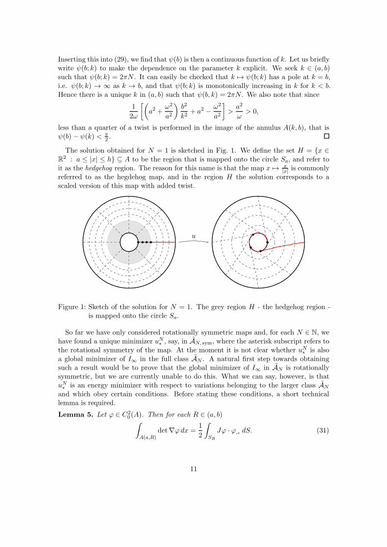
The solution obtained for N = 1 is sketched in Fig. 1. We define the set H = x ∈R2 : a ≤ |x| ≤ h ⊆ A to be the region that is mapped onto the circle Sa, and refer to

it as the hedgehog region. The reason for this name is that the map x 7→ x|x| is commonly

referred to as the hegdehog map, and in the region H the solution corresponds to ascaled version of this map with added twist.

u

Figure 1: Sketch of the solution for N = 1. The grey region H - the hedgehog region -is mapped onto the circle Sa.

So far we have only considered rotationally symmetric maps and, for each N ∈ N, wehave found a unique minimizer uN∗ , say, in AN, sym, where the asterisk subscript refers tothe rotational symmetry of the map. At the moment it is not clear whether uN∗ is alsoa global minimizer of I∞ in the full class AN . A natural first step towards obtainingsuch a result would be to prove that the global minimizer of I∞ in AN is rotationallysymmetric, but we are currently unable to do this. What we can say, however, is thatuN∗ is an energy minimizer with respect to variations belonging to the larger class AN

and which obey certain conditions. Before stating these conditions, a short technicallemma is required.

Lemma 5. Let ϕ ∈ C20 (A). Then for each R ∈ (a, b)ˆ

A(a,R)det∇ϕdx =

1

2

ˆ

SR

Jϕ · ϕ,τ dS. (31)

11

Proof. In the following we make use of the identity det∇ϕ = Jϕ,r ·ϕ,τ , where φ,τ = 1r∂ϕ∂θ

and (r, θ) are standard polar coordinates in two dimensions. It may also help to recallat this point that the 2× 2 matrix J is antisymmetric. For any R in the interval (a, b)

ˆ

A(a,R)det∇ϕdx =

ˆ R

a

ˆ 2π

0Jϕ,r · ϕ,θ dθ dr

= −

ˆ R

a

ˆ 2π

0(Jϕ,r),θ · ϕdθ dr

= −

ˆ 2π

0

ˆ R

a

(Jϕ,θ ),r · ϕdr dθ

= −

ˆ 2π

0Jϕ,θ (R, θ) · ϕ(R, θ) dθ +

ˆ 2π

0

ˆ R

a

Jϕ,θ · ϕ,r dr dθ

= −

ˆ

SR

Jϕ,τ · ϕdS −

ˆ

A(a,R)ϕ,τ · Jϕ,r dx.

We recognise the integrand of the rightmost term in the final line as det∇ϕ, whereupon(31) follows by rearranging the terms and observing that −Jϕ,τ · ϕ = ϕ,τ · Jϕ.

Proposition 6. Let N ∈ N and let uN∗ minimize I∞ in AN, sym.

(i) Let T+AN = ϕ ∈ W 1,20 (A) : uN∗ + ǫϕ ∈ AN for all sufficiently small ǫ > 0.

Then for each ϕ in T+AN

I∞(uN∗ + ǫϕ) ≥ I∞(uN∗ ) (32)

for all sufficiently small and positive ǫ.

(ii) Let v ∈ AN be such that ϕ := v − uN∗ satisfies

ˆ

H

|∇ϕ|2 + 2

(1 +

ω2

a2

)(1

k−

1

r

)det∇ϕdx ≥ 0.

ThenI∞(v) ≥ I∞(uN∗ ).

Proof. For brevity, let uN∗ = u in the following, and recall that D(u) =´

A|∇u|2 dx.

The proof of parts (i) and (ii) have a common beginning which relate the quantity´

A∇u · ∇ϕdx to terms involving cof ∇u · ∇ϕ. The former term is clearly of importance

when one considers the expansion

D(u+ ϕ) = D(u) + 2〈∇u,∇ϕ〉 +D(ϕ) (33)

and where one looks for conditions guaranteeing that (at least) one of 〈∇u,∇ϕ〉 andD(ϕ) + 〈∇u,∇ϕ〉 is nonnegative. Here 〈·, ·〉 is the L2(A) inner product.

12

First observe that since u is smooth on H and A \ H and its first derivatives arecontinuous across the boundary Sh, Green’s theorem implies that

ˆ

A

∇u · ∇ϕdx = −

ˆ

H

∆u · ϕdx (34)

Notice that, since u is harmonic on A\H, the domain of integration of the right-hand side

is the set H. Next, the specific form of the solution u implies that ∆u = − ar2

(ω2

a2+ 1)er,

so thatˆ

A

∇u · ∇ϕdx = a

(ω2

a2+ 1

)ˆ

H

1

r2er · ϕdx. (35)

Now, using the same notation as in the previous lemma, we can integrate cof ∇u · ∇ϕon A(a,R) for each fixed R ∈ (a, b) to obtain

ˆ

A(a,R)cof ∇u · ∇ϕdx =

ˆ

SR

(cof ∇u)n · ϕdS = a

ˆ

SR

er · ϕdS. (36)

Here, the specific form of the solution u has been used again: to be precise, one uses(19) to calculate cof ∇u = ρ

rer, which together with Piola’s identity div (cof ∇u) = 0 and

Green’s theorem yields the stated expression. The point we exploit below is that thequantity er ·ϕ appears in both (35) and (36), enabling us to control the term 〈∇u,∇ϕ〉using information about cof ∇u · ∇ϕ.

Proof of (i) Let ϕ belong to T+AN . Then for all sufficiently small ǫ > 0

det∇u+ ǫ cof ∇u · ∇ϕ+ ǫ2 det∇ϕ ≥ 0

a.e. in A, and since det∇u = 0 on H it is in particular true that

ǫ cof ∇u · ∇ϕ+ ǫ2 det∇ϕ ≥ 0

on H. Dividing by ǫ > 0 and letting ǫ → 0 yields cof ∇u · ∇ϕ ≥ 0 pointwise a.e. in H.From this and (36) it follows that

a

ˆ

SR

er · ϕdS ≥ 0

for R ∈ (a, h). Replacing R by r, multiplying the latter inequality by

ζ(r) :=

(ω2

a2+ 1

)1

r2

and integrating with respect to r over (a, k) implies, by (35), that 〈∇u,∇ϕ〉 ≥ 0. Hence,by replacing ϕ with ǫϕ in (33), we must have D(u+ ǫϕ) ≥ D(u) for all sufficiently smallǫ > 0. It follows that (32) must hold, which concludes the proof of part (i).

13

Proof of (ii) Let v ∈ AN be admissible and let ϕ = v − u. Since v is admissible anddet∇u = 0 a.e. on H, we can argue as above that

cof ∇u · ∇ϕ+ det∇ϕ ≥ 0

a.e. on H. Inserting this into (36) yields for each R ∈ (a, k) that

a

ˆ

SR

er · ϕdS ≥ −

ˆ

A(a,R)det∇ϕdx.

By a straightforward density argument we can suppose that ϕ is of class C20 (A). In

particular, we can apply Lemma 5 to deduce that

a

ˆ

SR

er · ϕdS ≥ −1

2

ˆ

SR

Jϕ · ϕ,τ dS.

Changing R to r, mutiplying both sides by ζ(r) , integrating with respect to r over (a, k)and recalling (35), it follows that

2〈∇u,∇ϕ〉 ≥ −

ˆ

H

ζ(r)Jϕ · ϕ,τ dx. (37)

The function ζ is a constant multiple of 1/r2, so we focus now on proving thatˆ

H

−1

r2Jϕ · ϕ,τ dx = 2

ˆ

H

(1

k−

1

r

)det∇ϕdx.

This can be seen as follows:ˆ

H

−1

r2Jϕ · ϕ,τ dx =

ˆ 2π

0

ˆ k

a

(1

r

)

,r

Jϕ · ϕ,θ dr dθ

=1

k

ˆ

Sk

Jϕ · ϕ,τ dS −

ˆ

H

1

rJϕ,r · ϕ,τ dx−

ˆ k

a

ˆ 2π

0

1

rJϕ · (ϕ,r),θ dθ dr

=2

k

ˆ

H

det∇ϕdx−

ˆ

H

1

rdet∇ϕdx+

ˆ

H

1

rJϕ,τ · ϕ,r dx

= 2

ˆ

H

(1

k−

1

r

)det∇ϕdx.

Hence

−

ˆ

H

ζ(r)Jϕ · ϕ,τ dx ≥ 2

(1 +

ω2

a2

)ˆ

H

(1

k−

1

r

)det∇ϕdx,

so that, by (37),

2〈∇u,∇ϕ〉 ≥ 2

(1 +

ω2

a2

)ˆ

H

(1

k−

1

r

)det∇ϕdx.

Inserting this into (33) gives

D(v) ≥ D(u) +

ˆ

H

|∇ϕ|2 + 2

(1 +

ω2

a2

)(1

k−

1

r

)det∇ϕdx+

ˆ

A\H|∇ϕ|2 dx,

from which the proof of part (ii) of the Proposition can easily be concluded.

14

This leads naturally to the following result that uN∗ is a minimizer of I∞ with respectto perturbations with suitably located support.

Corollary 7. Let N ∈ N and let uN∗ minimize I∞ in AN, sym. Let v ∈ AN be such thatϕ := v − uN∗ has support in the annulus A(r∗, b) ⊂ A, where

1

r∗=

1

k+

a2

a2 + ω2.

Then I∞(v) ≥ I∞(uN∗ ).

Proof. If sptϕ lies in A(r∗, b) as defined then a simple calculation shows that

∣∣∣∣(1 +

ω2

a2

)(1

k−

1

r

)∣∣∣∣ ≤ 1

for any r ≤ k such that Sr meets sptϕ. Hence, by Hadamard’s inequality, which in the2× 2 case is 2|detF | ≤ |F |2, the quantity

|∇ϕ|2 + 2

(1 +

ω2

a2

)(1

k−

1

r

)det∇ϕ

is pointwise nonnegative, and hence part (ii) of Proposition 6 implies that I∞(uN∗ +ϕ) ≥I(uN∗ ).

2.2 The case h = h0: twist minimizers with area compression energy

We now return to the case also considered by Post and Sivaloganathan [13]. We seek aminimizer of the functional

I0(u) =

ˆ

A

1

2|∇u|2 + h0(det∇u) dx (38)

for each N ∈ N, but where this time the local invertibility condition det∇u > 0 a.e. isencoded in the function h0 via the properties

(H1) h0 is convex with h0 ≥ 0

(H2) h0 ∈ C3((0,+∞)) and for some positive constants s, c1, c2 and d0, c1d−s−k ≤

(−1)kh(k)0 (d) ≤ c2d

−s−k for 0 < d < d0 and k = 0, 1, 2

(H3) h0(d) = +∞ for d ≤ 0

(H4) For some real number τ and positive constants c3, c4 and d1 c3dτ ≤ h′′0(d) ≤ c4d

τ

for d ≥ d1.

Again, instead of looking at the whole of AN , we focus on those functions in AN thatare rotationally symmetric, i.e. we minimize I0 on the set AN, sym defined in (13). Usingthe same notation as in the previous section, and by following [13], we conclude that the

15

rotationally symmetric minimizer uN∗ of I0 in AN, sym has radial and angular parts ρ, ψof class C2(a, b) and, moreover, that uN∗ solves the Euler-Lagrange equations, which forrotationally symmetric maps simplify to

[rρ+ ρh′0(d)

]′=ρ

r+ rρψ2 + ρh′0(d)

and

rρ2ψ = ω. (39)

In fact, since we assume slightly stronger conditions on h0 than Post and Sivaloganathando, we actually obtain that ρ ∈ C([a, b])∩C3(a, b). Since I0(u

N∗ ) < +∞, it is impossible

for det∇uN∗ to vanish on a set of positive measure. However, it may still be possible forρ(r) = 0 for some r (where r = a+ is understood on the inner boundary and r = b− onthe outer), which would correspond to det∇uN∗ (x) = 0 on the circle Sr. This was thecase for each r ∈ [a, h], for example, in the previous section of the paper. The followinglemma is motivated by the well-known works [4, 5].

Lemma 8. Let N ∈ N, let uN∗ minimize I0 in AN, sym and define the function f :(0,∞) → R by f(s) := sh′0(s) − h0(s). Define the functions d := det∇uN∗ and z :=12 |∇u

N∗ |2 + f(d) on the annulus A. Then d and z depend only on the radial variable

r, and d is strictly monotonically increasing on (a, b) while z is strictly monotonicallydecreasing on (a, b).

Proof. A direct calculation using the form of the solution uN∗ shows that d = ρρr, which

is clearly independent of the angular variable θ. The same us true of z, as is shown in(42) below. From the remarks above (concerning the regularity of ρ, essentially applying[13]) the quantities d and z are differentiable. Now assume for a contradiction that d ≤ 0.Then

ρ ≤1

ρ

(d− ρ2

). (40)

The Euler-Lagrange equations (39) are equivalent to

ρ

(r +

ρ2

rh′′0(d)

)=

1

r

(ρ+

ω2

ρ3

)− ρ+

ρ

r

(d− ρ2

)h′′0(d). (41)

The factor r + ρ2

rh′′0(d) is always positive, so we can use (40) on the left-hand side to

obtain

ρ+r

ρ

(d− ρ2

)≥

1

r

(ρ+

ω2

ρ3

)

Multiplying this through by ρrwe deduce that

−(ρ−

ρ

r

)2≥

ω2

r2ρ2,

16

which is impossible since ω 6= 0.For z we have, by direct calculation,

z =1

2

(ρ2 + ρ2ψ2 +

ρ2

r2

)+ f(d) =

1

2

(ρ2 +

ω2

r2ρ2−ρ2

r2

)+ f(d) +

ρ2

r2(42)

Differentiating and using (39) we find

z = −1

r

(ρ2 +

ω2

r2ρ2−ρ2

r2

)+ 2

ρρ

r2− 2

ρ2

r3

= −1

r

(ρ2 +

ω2

r2ρ2+ρ2

r2− 2

ρρ

r

)= −

1

r

((ρ−

ρ

r

)2+

ω2

r2ρ2

)< 0.

Now we are in the position to prove the following result, which asserts that det∇uN∗is bounded strictly away from 0 on A.

Lemma 9. Let N ∈ N and let uN∗ minimize I0 in AN, sym. Then if uN∗ is expressed inthe form

uN∗ (r, θ) = ρ(r)er(θ + ψ(r))

it holds that ρ ∈ C([a, b]) with ρ(a) > 0 and ρ(b) <∞.

Proof. Since d is monotonic on (a, b), the limits limr→a+ d(r) and limr→b− d(r) exist(possibly +∞ for r → b−). Therefore, the limits limr→a+ ρ(r) and limr→b− ρ(r) alsoexist, with the same qualification for the case r → b−. If ρ(r) were to vanish as r → a+then we would have d → 0+ as r → a+, and hence f(d) = dh′0(d) − h0(d) would tendto −∞ as r → a+. Recalling (42), it follows that z(r) → −∞ as r → a+. On theother hand, z(r) is decreasing on (a, b) and certainly finite on that interval, implying inparticular that limr→a+ z(r) is not −∞, which is a contradiction. Hence ρ(a+) is strictlypositive. The argument needed to show that ρ(b−) <∞ is similar.

We remark, in passing, that we are able to derive the following maximum principle.

Theorem 10. Let uN∗ satisfy the hypotheses of Lemma 9. Then the function ρrattains

no interior local maximum. In particular,(ρr

)·· changes sign only once and ab≤ ρ

r< 1

in (a, b) with ρr= 1 at a, b.

Proof. Assume there exists an r ∈ (a, b) s.t.(ρr

)· = 0 and(ρr

)·· ≤ 0. Then

0 ≥(ρr

)··= −

2

r

(ρr

)·+

1

rρ =

1

rρ. (43)

However, by Theorem 8 we have

0 < d =1

r

(ρ2 + ρρ− d

)=ρ

rρ+ ρ

(ρr

)·=ρ

rρ (44)

which contradicts (43).

17

3 Shear maps

In this section we focus on so-called shear maps and their properties. In brief, for anygiven domain D ⊂ R

n a shear map uσ : D → Rn takes the form

uσ(x) = x+ σ(x)e,

where e is a fixed unit vector in Rn and the function σ is real-valued. We echo some

of the constructions of Section 2 by posing and then solving variational problems firstin the case that the weak constraint det∇uσ ≥ 0 is required to hold, that is whenh = h∞, and then in the case that compression to zero ‘area’ is energetically penalized,corresponding to h = h0. In the former case, and still in a two dimensional setting, wefind conditions which imply that the unique minimizer of a Dirichlet energy among shearmaps necessarily satisfies det∇uσ = 0 on a specified subdomain. (Cf. Section 2.1 andthe ‘hedgehog map’.) Moreover, we establish conditions under which the global energyminimizer fails to be C1 at interior points of the domain. The conditions are based oneasily verifiable boundary behaviours of functions harmonic on certain subdomains of D.See Section 3.1 for details.

Where the stronger constraint det∇uσ > 0 a.e. is required to hold, via I0(uσ) < +∞,we find that even if compression is strongly energetically penalized7, circumstances arisein which the unique energy minimizing shear map fails to be C1. In this case the gradientis discontinuous ‘at’ certain boundary points. See Section 3.2 for details.

Our chief ally in proving these assertions is the fact that the Jacobian of any shearmap uσ is linear in ∇σ, viz.

det∇uσ = 1 + e · ∇σ.

Consequently, the Jacobian of a convex combination of any two shear maps uσ1 and uσ2

satisfiesdet∇uλσ1+(1−λ)σ2

= λdet∇uσ1 + (1− λ) det∇uσ2 ,

where 0 ≤ λ ≤ 1. In particular, it follows that if the maps uσiobey the constraint

det∇uσi≥ 0 for i = 1, 2 then any convex combination must also obey that constraint.

Moreover, inserting F = ∇uσ into the general form stored-energy function W (F ) =12 |F |

2 + h0(detF ), we find that

W (∇uσ) =1

2|1+ e⊗∇σ|2 + h0(1 + e · ∇σ)

is in fact convex in ∇σ. This convexity turns out to be useful in both the weak andstrong constraint cases (corresponding, respectively to the choice h = h∞ and h = h0).When the weaker constraint det∇σ ≥ 0 a.e. holds, it means that all we need do toestablish that a given admissible map is a minimizer is to prove that it is a solution ofa variational inequality associated with the energy functional

Iw(σ) :=

ˆ

Ω|∇uσ|

2 dx, (45)

7This is achieved by requiring in addition that det∇uσ ≥ c > 0 a.e. in the domain.

18

whereas when the strong constraint det∇uσ > 0 is in force the convexity of W (∇uσ) in∇σ allows us to apply elliptic regularity theory under certain conditions, an importantintermediate step in determining the behaviour of ∇uσ near the boundary.

3.1 The case h = h∞: shear minimizers without area compression energy

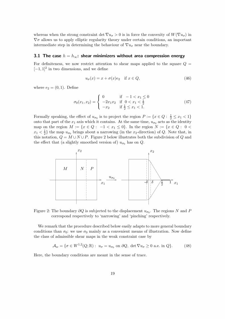
For definiteness, we now restrict attention to shear maps applied to the square Q =[−1, 1]2 in two dimensions, and we define

uσ(x) = x+ σ(x)e2 if x ∈ Q, (46)

where e2 = (0, 1). Define

σ0(x1, x2) =

0 if − 1 < x1 ≤ 0−2x1x2 if 0 < x1 <

12

−x2 if 12 ≤ x1 < 1.

(47)

Formally speaking, the effect of uσ0 is to project the region P := x ∈ Q : 12 ≤ x1 < 1

onto that part of the x1 axis which it contains. At the same time, uσ0 acts as the identitymap on the region M := x ∈ Q : −1 < x1 ≤ 0. In the region N := x ∈ Q : 0 <x1 <

12 the map uσ0 brings about a narrowing (in the x2-direction) of Q. Note that, in

this notation, Q =M ∪N ∪P . Figure 2 below illustrates both the subdivision of Q andthe effect that (a slightly smoothed version of) uσ0 has on Q.

x1x1

x2x2

M N P

uσ0

12

1δ-δ

Figure 2: The boundary ∂Q is subjected to the displacement uσ0 . The regions N and Pcorrespond respectively to ‘narrowing’ and ‘pinching’ respectively.

We remark that the procedure described below easily adapts to more general boundaryconditions than σ0: we use σ0 mainly as a convenient means of illustration. Now definethe class of admissible shear maps in the weak constraint case by

Aw = σ ∈W 1,2(Q;R) : uσ = uσ0 on ∂Q, det∇uσ ≥ 0 a.e. in Q. (48)

Here, the boundary conditions are meant in the sense of trace.

19

Lemma 11. Let Iw and Aw be defined by (45), (48) respectively. Then Iw has a uniqueglobal minimizer in Aw. In particular, the global minimizer σw of Iw in Aw satisfies theinequality

ˆ

Q

∇σ · ∇η dx ≥ 0 (49)

for all η ∈W 1,2(Q;R) such that σ + η belongs to Aw.

Proof. To prove the first assertions of the lemma it suffices to show that Aw is nonemptyand closed under weak convergence in W 1,2(Q,R) and then to apply the direct methodof the calculus of variations.

A short calculation shows that

det∇uσ0(x) =

1 if x ∈M1− 2x1 if x ∈ N0 if x ∈ P,

where M , N and P are as defined above. Since 0 ≤ det∇uσ0 = 1 + σ0,2 a.e., it followsfrom standard properties of mollifiers that 1+σ0,2 ≥ 0 a.e. in Q. Therefore det∇σ0 ≥ 0a.e. in Q, and so σ0 is admissible. In particular, Aw is nonempty.

Now let σ(j) be a sequence in Aw converging weakly to σ. Properties of the trace implythat σ satisfies the same boundary conditions as all the σ(j), and since det∇uσ(j) =1+σ(j),2

≥ 0 a.e. in Q for all j, it easily follows that det∇uσ ≥ 0 a.e. in Q also. Thus Aw

is weakly closed. The convexity of Iw with respect to σ coupled with the direct methodthen yields the existence of σw minimizing Iw in Aw. The minimizer is unique becausethe functional Iw is strictly convex and the class Aw is convex.

We now prove that (49) is necessary and sufficient for σ to minimize Iw in Aw. Letη ∈W 1,2(Q;R) be such that σ+ η ∈ Aw, and let σ minimize Iw in Aw. Then by writing

σ + ǫη = ǫ(σ + η) + (1− ǫ)σ

and noting that the right-hand side clearly belongs to Aw provided 0 ≤ ǫ ≤ 1, it followsby minimality that I(σ + ǫη) ≥ Iw(σ) for all such ǫ. Now,

Iw(σ) =

ˆ

Q

|1+ e2 ⊗ (∇σ)|2 dx,

so that∂ǫ|ǫ=0Iw(σ + ǫη) ≥ 0

yields the inequalityˆ

Q

η,2 +∇σ · ∇η dx ≥ 0 (50)

for all such η. Applying the boundary condition η|∂Q = 0 to this gives (49). Note that(49) is a sufficient condition for the minimality of σ in Aw. This follows immediatelyfrom the identity

Iw(σ + η) = Iw(σ) +

ˆ

Q

|∇η|2 + 2η,2 + 2∇σ · ∇η dx.

20

The next result shows that any element σ of Aw satisfies det∇uσ(x) = 0 a.e. on P ,which is in accordance with physical intuition where the region is severely ‘pinched’.

Lemma 12. Let σ belong to Aw. Then

σ0(x1,−1)− 1− x2 ≤ σ(x) ≤ σ0(x1, 1) + 1− x2 (51)

for a.e. x in Q. In particular, σ(x) = −x2 for a.e. x in P , so that det∇uσ = 0 a.e. onP .

Proof. For a.e. x1 in (−1, 1) it holds that

σ(x1, 1)− σ(x1, x2) =

ˆ 1

x2

σ,2(x1, t) dt

for a.e. x2 in (−1, 1). Applying the constraint σ,2 ≥ −1 and the boundary conditiongives

σ(x) ≤ σ0(x1, 1) + 1− x2

a.e. x in Q. Arguing similarly, using the boundary condition at points of the form(x1,−1), we obtain the left-hand inequality in (51). The last assertion of the lemmafollows by observing that σ0(x1,±1) = ∓1 when x1 ∈ (12 , 1).

There is an interesting and quite subtle interaction between the solution σ(x) = −x2on the region P with its possible behaviour elsewhere on the domain. This yields a testfor whether the constraint 1+σ,2 ≥ 0 a.e. becomes an equality on a set of positive measurein the subdomain Q\P . In other words, it is possible to test whether det∇uσ = 0 holdson a set of positive measure away from the pinched part P of the domain Q, where, byLemma 12, the vanishing of the Jacobian is automatic for all competitors σ in Aw.

Lemma 13. Let σ minimize Iw in Aw and define

Ω := Q \ P. (52)

Then at most one of

(i) ess inf1 + σ,2(x) : x ∈ U > 0 for all U ⊂ Ω with measU > 0, and

(ii)´ 1−1 φ(x2)σ,1(1/2, x2) dx2 = 0 for all φ ∈ C1

c ((−1, 1)).

is true.

Proof. Suppose for a contradiction that both (i) and (ii) hold. Let B(y, δ) ⊂ Ω and takeϕ ∈ C1

c (B(y, δ),R). Then, since by hypothesis there is c > 0 such that 1 + σ,2(x) ≥ cfor a.e. x in B(y, δ), it is the case that σ + ǫϕ belongs to Aw for all sufficiently small ǫ.Arguing as in the prelude to (49), it follows that

ˆ

Ω∇ϕ · ∇σ dx = 0, (53)

21

and hence by standard theory, that σ is harmonic on the open set Ω.Next, let Φ ∈ C1

c (Q,R) and note that, since the set K := ∂P ∩ ∂Ω has (two-dimensional) Lebesgue measure zero, it follows from (53), the final assertion of Lemma12 (which implies that σ = −x2 on P ) and Green’s theorem that

ˆ

Q

∇Φ · ∇σ dx =

ˆ

K

Φ (1/2, x2) σ,1 (1/2, x2) dx2 −

ˆ

P

Φ,2 dx.

Since Φ has compact support in Q, the second integral on the right-hand side vanishes.Therefore, since we are assuming that (ii) holds, the previous line implies that

´

Q∇Φ ·

∇σ dx = 0 for all Φ ∈ C1c (Q), and hence that σ is harmonic on Q. But σ = −x2 on P

by Lemma 12 and hence, since σ is harmonic on Q ⊃ P and P has a nontrivial interior,it follows that σ = −x2 on all of Q. This requirement violates the boundary conditions,which is a contradiction.

Proposition 14. Let σ0 be as defined in (47) and let Σ be the unique harmonic functionagreeing with σ0 on ∂Ω, where Ω = Q \ P is defined in (52). Then

σ(x) =

Σ(x) if x ∈ Ω−x2 if x ∈ P

is the unique global minimizer of Iw in Aw and det∇uσ > 0 everywhere in Ω. It alsoholds that σ,1 cannot vanish H1-a.e. along the set K = y ∈ Q : y1 = 1/2. In particular,the global minimizer does not belong to the class C1(Q).

Proof. The first part of the proof consists in showing that σ is admissible and thatdet∇uσ > 0 in Ω: this is done in Steps 1− 3. Steps 4 and 5 deal respectively with thelast two sentences in the statement of the Proposition.

Step 1 By standard results in the theory of harmonic functions, σ agrees with σ0 inthe sense of trace on ∂Q, so it only remains to prove that 1 + σ,2 ≥ 0 a.e. in Ω, thisfact being immediate in P . Consider z1(x) = 1 − x2 and note that Σ(x) ≤ z1(x) for allx ∈ ∂Ω. Since z1 is harmonic and both functions belong toW 1,2(Ω), the weak maximumprinciple implies that Σ(x) ≤ z1(x) for all x ∈ Ω. In particular, Σ(x1, 1 + h) ≤ −h for−1 < h < 0 and −1 ≤ x1 ≤ 0. Therefore, since Σ(x1, 0) for −1 ≤ x1 < 0, we have

Σ(x1, 1 + h)− Σ(x1, 1)

h≥ −1

for this range of x1 and h, so that letting h → 0 gives Σ,2(x1, 1) ≥ −1. A similarargument using the harmonic function −1− x2, which satisfies z2(x) ≤ Σ(x) for x ∈ ∂Ω,implies that Σ,2(x1,−1) ≥ −1 for −1 ≤ x ≤ 0. The derivatives Σ,2(x1, 1) and Σ,2(x1,−1)for 0 ≤ x1 ≤ 1/2 can be bounded below by −1 in a similar fashion, the only differencesbeing that the comparison function z1 should be replaced by z1(x)−2x1 in the first caseand z2(x) by z2(x) − 2x1 in the second. It is immediate from the boundary conditionthat 1 + Σ,2(±1, x2) ≥ 0, so that, in summary, 1 + Σ,2 ≥ 0 on all of ∂Ω.

Step 2 Now note that 1+Σ,2 is harmonic in Ω, so that if Σ,2 were to belong to W 1,2(Ω)then the weak maximum principle would apply. This, together with the previously

22

established fact that 1 + Σ,2 ≥ 0 on ∂Ω would then imply 1 + Σ,2 ≥ 0 on Ω, and hencethat σ belongs to Aw as desired. By [9, Theorem 8.12], Σ belongs to W 2,2(Ω′), whereΩ′ is any subset of Ω whose closure does not contain the corners (−1,±1), (1/2,±1) orthe points (0,±1). The reason is that away from these points the boundary conditionΣ = σ0 is smooth and the (flat) boundary is sufficiently regular. In particular, it followsthat Σ,2 belongs to W 1,2(Ω′) for such Ω′ and the weak maximum principle will apply.We have already established that 1 + Σ,2 ≥ 0 on ∂Ω, but it could still be that, for somec > 0, 1 + Σ,2 < −c occurs in Ω and persists ‘up to the corners’: the argument we givebelow rules this out.

To fix ideas, let ǫ > 0, let C = (−1,±1), (1/2,±1), (0,±1) and define Ωǫ = Ω \∪a∈CB(a, ǫ). Thus Ωǫ is a version of Ω with small neighbourhoods of the set C removed.Each point a in C has now given rise to two distinct corners a1 and a2, say, on ∂Ω, butit is easy to smoothen ∂Ωǫ near the newly created corners, thereby producing a newsubset Ω′

ǫ, say, of Ωǫ with the properties that (i) ∂Ω′ǫ is smooth and (ii) ∂Ω′

ǫ agrees with∂Ω except possibly in sets of the form B(a, 2ǫ), where a lies in C. Thus

∂Ω \ ∂Ω′ǫ =

⋃

a∈C

Γǫa

where each Γǫa is a smooth curve whose maximum distance from ∂Ω is of order 2ǫ.

Claim: for each a in C it is the case that

lim infǫ→0

infΓǫa

(1 + Σ,2) ≥ 0.

Proof of claim: in the notation of Lemma 20, let E = x ∈ Ω : Σ,2(x) + 1 < 0.Without loss of generality let a = (−1, 1) and let z ∈ Γǫ

a. Suppose that Σ,2(z) + 1 < 0and for any y in Ω let Py = (y1, 1), that is, Py is the projection of y onto the upperboundary of Ω. Since Σ is smooth on compact subsets of Ω, for any y in Ω there existsa first point y1(y) on the line [y, Py] where F := Σ,2 + 1 satisfies F (y1(y)) ≥ 0. Inparticular, [y, y1(y)) ⊂ E. Note that |y−y1(y)| ≤ d(y) := dist(y, ∂Ω). Then we estimateF (y) from below as follows:

F (y) =

ˆ 1

0∇F ((1− t)y + ty1(y)) · (y1(y)− y) dt

≥ −d(y)

ˆ 1

0|∇F ((1− t)y + ty1(y))| dt.

Now let 0 < r < 12d(z) and integrate over B(z, r) ⊂ Ω. Note that the bounds d(z)/2 <

d(y) < 3d(z)/2 are immediate for y ∈ B(z, r). Since F is harmonic, the mean valuetheorem applies, so that

F (z) ≥ −3d(z)

2πr2

ˆ

B(z,r)

ˆ 1

0|∇F ((1− t)y + ty1(y))| dt dy

≥ −Cd(z)

r

(ˆ

T

|∇F |2 dy

) 12

23

using Holder’s inequality, where C is a positive constant that does not depend on thequantities elsewhere in the estimate. Here, the set T ⊂ E is formed from the unionof lines [y, y1(y)] where y ∈ B(z, r) and, by inspection, its measure is at most of orderrd(z). Now suppose we fix r = d(z)/2: then the measure of T is bounded above by aquantity of order d(z)2 ≤ 4ǫ2. Hence the estimate above gives

F (z) ≥ −2C

(ˆ

T

|∇F |2 dy

) 12

.

Since T ⊂ E, Lemma 20 applies and ensures that the integral on the right tends to 0 asǫ→ 0. This proves the claim.

To conclude Step 2 we apply the weak maximum principle to the domain Ω′ǫ defined

above, giving for each a ∈ C

Σ,2(x) + 1 ≥ min

0, inf

Γǫa

1 + Σ,2

∀x ∈ Ω′

ǫ.

Letting ǫ→ 0 and applying the claim above, we see that Σ,2(x) + 1 ≥ 0 for any x ∈ Ω.

Step 3 We apply the strong maximum principle to establish that Σ,2(x) + 1 > 0 in Ω.Suppose for a contradiction that there is x∗ in Ω such that Σ,2(x

∗) + 1 = 0. Pick a

subdomain Ω = (−1, 1/2) × (1− s,−1 + s) containing x∗ and where s > 0. Notice thatΣ,2(1/2, x2)+1 = 0 for |x2| < 1, so that x∗ would be an interior minimum for Σ,2+1 and

Σ lies in W 2,2(Ω). By the strong maximum principle, this is only possible if Σ,2 + 1 = 0throughout Ω. But this violates the boundary condition Σ(−1, x2) = 0 for |x2| < 1.

Step 4 Next, we show that σ as defined satisfies inequality (49), which, by Lemma 11,is both necessary and sufficient for Ω to minimize Iw in Aw. Let η ∈ W 1,2

0 (Q) be suchthat σ + η ∈ Aw. Let η(j) approximate η in W 1,2 norm, where η(j) ∈ C∞

c (Q) for all j.By construction, σ is harmonic on each of the subsets Ω and P , so that, arguing as inthe proof of Lemma 13,

ˆ

Q

∇η(j) · ∇σ dx =

ˆ

K

η(j)σ,1 dH1 −

ˆ

P

η(j),2dx

The second integral on the right-hand side vanishes trivially. To deal with the integralalong K = ∂Ω ∩ ∂Ω we note that, by Lemma 12, we must have η|Lx1

= 0 on almostevery part line Lx1 = x1 × [−1, 1] in P . Therefore, without loss of generality, we mayassume that η|K = 0. Moreover, since η(j) → η in particular in W 1,2(Ω), properties ofthe trace imply that η(j) → 0 in L2(K). By construction, σ,1 is bounded on Q, so itfollows that

´

Kη(j)σ,1 dH

1 → 0 as j → ∞. Hence inequality (49) holds as an equality,and it follows from Lemma 11 that σ as constructed is the global minimizer of Iw in Aw.

Step 5 The final assertion of the proposition follows by applying Lemma 13. Indeed,alternative (i) of that lemma holds because, as we have seen, det∇uσ is strictly positiveand continuous on Ω. Therefore alternative (ii) cannot hold, meaning that σ,1 is notzero when viewed as the trace of σ,1 |Ω along K. Since σ,1 clearly vanishes in P , it cannotbe that ∇σ is continuous across K. This concludes the proof.

24

Remark 15. The last line of the statement of the proposition could be anticipated bynoting that σ maps the set K to a point. Therefore in any left-neighbourhood of K, withobvious notation, the derivative σ,1 could not possibly agree with the same derivative inthe region P .

3.2 The case h = h0: shear minimizers with area compression energy

In this section we examine the effect of imposing the constraint det∇uσ > 0 a.e. in Q.We focus in particular on a problem where a displacement boundary condition is appliedacross a strict subset

∂Q1 = x ∈ ∂Q : x = (±1, x2), |x2| ≤ 1 (54)

of ∂Q. On the ‘free boundary’ ∂Q\∂Q1 a natural so-called traction-free condition shouldarise, but this is not straightforward since it involves the first derivatives of σ and theseare not necessarily defined even in the sense of trace on ∂Q. We make sense of this byimposing on the minimizing σ the additional condition 1 + ∂2σ ≥ c > 0 a.e. in Q forsome constant c, that is we strengthen det∇uσ > 0 a.e. in Q to det∇uσ ≥ c > 0 a.e. inQ. The convexity of W (∇uσ) in ∇σ then allows us to apply a bootstrapping argumentto improve the regularity of σ to W 2,2(Q), so that the natural boundary condition iswell-defined via the trace theorems for Sobolev functions.

One outcome of this is that σ satisfying these assumptions cannot be C1(Q): the‘corner’ of the domain together with the natural and imposed boundary conditions com-bine to form a discontinuity in the gradient ‘at’ the corner. On closer inspection thesame phenomenon could be induced by considering a suitable Neumann problem for theDirichlet energy on the same domain and with the same boundary conditions. Moreinteresting is its interpretation in the original nonlinear elasticity setting, namely thatif a minimizer is such that det∇uσ is bounded away from zero a.e. then it is not C1(Q).This seems strange because one normally thinks of the condition det∇uσ ≥ c > 0 a.e. asbeing ‘regularizing’, and indeed we shall see that it is so at interior points of the domain.We have to conclude that the free boundary ∂Q2 := ∂Q \ ∂Q1 plays a significant role inproducing the discontinuity in ∇σ ‘at’ the boundary.

We now give the details of the results alluded to above. Let

Is(σ) =

ˆ

Q

1

2|∇uσ|

2 + h0(det∇uσ) dx, (55)

where, for concreteness, we assume that h0 satisfies hypotheses (H1)-(H3). Let ∂Q± =(±1, t) : −1 ≤ t ≤ 1 denote the left (-) and right (+) sides of Q, and let σ1 be anyW 1,2(Q;R) map such that Is(σ1) < +∞. Finally, define the class of admissible maps inthe strong constraint case by

As = σ ∈W 1,2(Q;R) : uσ = uσ1 on ∂Q+ ∪ ∂Q−, Is(σ) < +∞. (56)

Note that, in the notation introduced above, ∂Q1 = ∂Q+ ∪ ∂Q−.

25

Proposition 16. Let Is and As be defined as in (55) and (56) respectively. Then thereexists a minimizer of Is in As.

Proof. By hypothesis, As contains σ1 and is thus nonempty. The integrand of the func-tional Is is polyconvex and, moreover, satisfies the hypotheses of [3, Theorem 6.1] in thetwo dimensional case. Hence I(u) :=

´

QW (∇u) dx is sequentially lower semicontinuous

with respect to weak convergence in W 1,2(Q;R2). Let uσ(j) be a minimizing sequencewhich without loss of generality we can suppose to be weakly convergent to u, say. Itis straightforward to show that u = uσ for some σ, i.e. u is a shear map, and, by thesequential weak lower semicontinuity of I(·), that σ minimizes Is in As.

For concreteness we fix σ1 = 0, so that σ = 0 (in the sense of trace) on ∂Q1 for any σin As. This corresponds to applying the boundary condition uσ = id on ∂Q1. It is clearthat σ1 is such that I(σ1) < +∞.

We also impose a further condition on the convex function h0: namely, that theupper bound in condition (H4) defined in Section 2.2 holds with the parameter τ0 = 0.Alternatively, we can (and do) impose the following condition:

∀µ > 0 ∃Cµ > 0 ∀s ∈ [µ,+∞) |h′′0(s)| ≤ Cµ. (57)

This, together with the next lemma, will allow us to apply some elliptic regularity theorytechniques.

Lemma 17. Let the C2 function h0 satisfy hypothesis (57). Then for each µ > 0 thereis C ′

µ > 0 such that |h′0(s)| ≤ C ′µs for all s ≥ µ.

Proof. Using hypothesis (57) and the assumption that h0 is C2, it is straightforward tocheck that

|h′0(s)| ≤ |h′0(µ)|+ Cµ|s− s0|

provided s ≥ µ. Therefore

|h′0(s)| ≤

(2Cµ +

|h′0(µ)|

µ

)s

for all s ≥ µ, and the lemma follows.

We are now in a position to improve the regularity of the minimizing map σ. In therest of this section it will be convenient to switch notation, writing ∂1σ in place of σ,1 ,and so on.

Lemma 18. Let W be given by (3) with h = h0 and assume that h0 is strongly convex,C2 where it is finite, and that it satisfies (H1) - (H3) and (57). Then the function

∇σ 7→ W (∇uσ)

is strongly convex and the minimizer σ of Is in As is unique. Moreover, if there existsc > 0 such that

1 + ∂2σ(x) ≥ c a.e. x ∈ Q (58)

then σ belongs to W 2,2(Q \ V ) where V is any compact set whose interior contains thecorners (±1,±1) of Q.

26

Proof. The first assertion of the lemma is straightforward when we see that the convexityof

W (∇uσ) =1

2|1+ e2 ⊗∇σ|2 + h0(1 + ∂2σ)

with respect to ∇uσ is equivalent to the strong ellipticity of the system (59) introducedbelow, so in anticipation of that result we do not prove strong convexity here.

If there were two distinct minimizers of Is in As, σ and σ, say, with Is(σ) = Is(σ) = m,then the strict convexity of W (∇uσ) in ∇σ coupled with the convexity of the class As

clearly implies thatIs(σ/2 + σ/2) < m,

a contradiction. Thus σ is unique.Now suppose that condition (58) holds. Then if η is any smooth function with compact

support in Q it follows that σ + ǫη is admissible provided ǫ is sufficiently small. Hence,on using a suitable dominated convergence theorem, it can be checked that ∂ǫIs(σ+ ǫη)vanishes at ǫ = 0, leading to

ˆ

Q

L(∇σ) · ∇η dx = 0, (59)

whereL(p) = (p1, 1 + p2 + h′(1 + p2)) ∀p ∈ R

2.

The hypotheses on h together with assumption (58) imply that (59) is an elliptic systemsatisfying controllable growth conditions. To see this, note that by the convexity of h0and (58),

ξTDL(p)ξ = ξ21 + (1 + h′′0(1 + p2))ξ22 ≥ λ|ξ|2

for some λ > 0 and all ξ ∈ R2. Moreover, by (58) and Lemma 17, |L(p)| ≤ C|p| for all p

such that 1+p2 ≥ c. A differencing argument, such as the one given in the course of theproof of [8, Theorem 1.1, Chapter II], can now be employed to prove that D2σ ∈ L2

loc.In fact, the argument leading to [8, Proposition 3.1, Chapter VI] shows that σ belongsto W 2,q(Q,R) for some q > 2 (this makes use of reverse Holder inequalities derived fromthe elliptic system (59)). In particular, ∇σ is Holder continuous on any compact subsetof Q. Moreover, (59) can now be written as

∂21σ + (1 + h′′0(1 + ∂2σ))∂22σ = 0 a.e. in Q. (60)

It will be useful below to note that the strong convexity of h together with Lemma17 and assumption (58) imply that there are positive constants c1 and c2 such thatc1 ≤ h′′0(1 + ∂2σ(x)) ≤ c2 holds on Q.

The regularity asserted in the lemma is W 2,2(Q \ V ), where V is described above, sowe must consider the behaviour near boundary points. Let x0 ∈ ∂Q be such that x0 /∈ V .If x0 ∈ ∂Q1 where the boundary condition σ = 0 is applied, then one can proceed asin the proof of [9, Theorem 8.12]. Specifically, differencing shows that both ∂2∂1σ and∂22σ belong to L2(B(x0, r) ∩ Q) for all sufficiently small r. Equation (60) then impliesthat ∂21σ also belongs to L2(B(x0, r) ∩ Q). The argument needed when x0 belongs to

27

∂Q2 = ∂Q \ ∂Q1 is similar. A covering argument now implies that D2σ belongs toL2(Q \ V ), as required.

Proposition 19. Let W be given by (3) satisfy all the assumptions of Lemma 18, andin addition suppose that 1 + h′0(1) 6= 0. Let σ be the unique minimizer of Is in As andsuppose there is a constant c > 0 such that 1 + ∂2σ(x) ≥ 0 for a.e. x in Q. Then ∇σ isnot continuous at the corners of Q.

Before giving the proof we remark that the condition 1 + h′0(1) 6= 0 is tailored to thechoice of Dirichlet boundary condition σ = 0 on ∂Q1. In general, one could easily adaptthe condition on h′0, which is not especially restrictive, to reflect a different choice ofboundary condition.

Proof. By Lemma 18 and properties of the trace for Sobolev functions, the trace of ∇σbelongs to L2(A) where A is any measurable subset of ∂Q whose closure does not containthe corners of Q. Green’s theorem can now be applied to (59), yielding

ˆ

∂Q2

L(∇σ) · ν η dH1 = 0

for any η whose compact support does not meet ∂Q1, where ν is ±e2 are the only twopossible outward pointing normals. In particular, it follows that

L2(∇σ) = 0 a.e. on ∂Q2,

that is1 + ∂2σ(x1,±1) + h′0(∂2σ(x1,±1) + 1) = 0 a.e. x1 ∈ (−1, 1). (61)

On the other hand, the boundary condition on ∂Q1 implies

1 + ∂2σ(±1, x2) + h′0(∂2σ(±1, x2) + 1) = 1 + h′0(1) a.e. x2 ∈ (−1, 1). (62)

Therefore if ∇σ were continuous at the corner (1, 1), say, then

limx1→1

1 + ∂2σ(x1, 1) + h′0(∂2σ(x1, 1) + 1) = limx2→1

1 + ∂2σ(1, x2) + h′0(∂2σ(1, x2) + 1)

would necessarily hold, which is impossible because the left-hand side is 0 by (61) andthe right-hand side is 1 + h′0(1) 6= 0 by (62) and the hypothesis on h′0(1).

Appendix

The following result is needed in the proof of Proposition 14.

Lemma 20. Let Ω = (−1, 1/2)× (−1, 1) and define σ0 as per (47). Let Σ be the uniqueharmonic function agreeing with σ0 on ∂Ω, and let E = y ∈ Ω : 1 + Σ,2(y) < 0.Then ∇Σ,2 belongs to L2(B(a, γ)∩E), where 0 < 2γ < 1/4 and a is any point in the setC := (−1,±1), (1/2,±1), (0,±1).

28

Proof. We deal first with the case that a is a corner of Ω, and without loss of generalitytake a = (−1, 1). Since Σ(x) = 0 for x ∈ B(a, 2γ)∩∂Ω, we may extend Σ by zero outsideΩ. Let η ∈ C1

c (B(a, 2γ)) and define the test function

ϕ(x) = η2(x)min∆2,hΣ(x) + 1, 0 (A.1)

for x ∈ Ω and h ∈ (−h0, h0), where h0 is suitably small. Here,

∆2,hΣ(x1, x2) =Σ(x1, x2 + h)− Σ(x1, x2)

h

is the difference quotient in the e2 = (0, 1) direction. According to the proof of Proposi-tion 14, Σ(x1, 1+h)−Σ(x1, 1) ≤ −h for h < 0, so that in particular ∆2,hΣ(x1, 1)+1 ≥ 0.For positive h the difference quotient is zero, so it follows that ∆2,hΣ(x1, 1) + 1 ≥ 0for −h0 < h < h0 and hence that ϕ(x) = 0 for x ∈ B(0, 2γ) ∩ ∂Ω. Thus ϕ ∈W 1,2

0 (B(0, 2γ) ∩ Ω) and since Σ is harmonic in this set we must have 〈∇Σ,∇ϕ〉 = 0,where 〈·, ·〉 is the L2(Ω) inner product. The standard procedure is now to ‘difference’this inner product, which leads to

ˆ

Ω∆2,h(∇Σ) · ∇ϕdx = 0.

Inserting ϕ and applying standard inequalities (see, for example, the proof of [9, Theorem8.12]), we obtain

ˆ

Ωη2|∆2,h(∇Σ)|2χ2

Eh dx ≤ C

ˆ

Ω|∇η|2|∆2,hΣ+ 1|2χ2

Eh dx (A.2)

for some constant C that is independent of Ω, h and Σ, and where Eh = y ∈ Ω :∆2,hΣ(y) + 1 < 0 and χEh its characteristic function.

Now let y ∈ E. Since Σ is harmonic it is smooth in Ω, so it follows that there is ρy > 0and hy > 0 such that B(y, ρy) ⊂ Eh for all h ∈ (−hy, hy). In particular, χEh → χE

pointwise almost everywhere in B(0, 2γ) ∩ Ω. Take η to be a cut-off function satisfyingη(z) = 1 if z ∈ B(a, γ) and |∇η| ≤ c/γ for some fixed constant c. Using this andNirenberg’s Lemma (see [9, Lemma 7.24], for example), we obtain from (A.2) that

ˆ

E

η2|∇Σ,2 |2 dx ≤

C ′

γ2

ˆ

B(a,2γ)\B(a,γ)1 + |∇Σ|2 dx.

This proves the lemma in the case that a is a corner of Ω.Now suppose a = (0, 1), let η be as above and extend Σ by zero outside Ω in the

region x ∈ R2 : x1 < 0 and by −2x1 in the region x ∈ Ω : x1 > 0, that is we let

Σ(x1, x2) = σ0(x1, 1) if x2 > 1. Using the same test function as defined in (A.1) togetherwith the fact established in Proposition 14 that Σ(x1, 1 + h)− σ0(x1, 1) ≤ −h for h < 0,it again follows that ∇Σ,2 ∈ L2(B(a, γ)∩E). This concludes the proof of the lemma.

29

References

[1] J. Ball. Minimizers and the Euler-Lagrange equations. In P. Ciarlet and M. Roseau,editors, Trends and Applications of Pure Mathematics to Mechanics, volume 195 ofLecture Notes in Physics, pages 1–4. Springer Berlin Heidelberg, 1984.

[2] J. M. Ball. Some open problems in elasticity. In P. Newton, P. Holmes, andA. Weinstein, editors, Geometry, Mechanics, and Dynamics, pages 3–59. SpringerNew York, 2002.

[3] J. M. Ball and F. Murat. w1,p−quasiconvexity and variational problems for multipleintegrals. Journal of Functional Analysis, 58(3):225–253, 1984.

[4] P. Bauman, N. C. Owen, and D. Phillips. Maximum principles and a priori estimatesfor a class of problems from nonlinear elasticity. Annales de l’institut Henri Poincare(C) Analyse non lineaire, 8(2):119–157, 1991.

[5] P. Bauman, D. Phillips, and N. C. Owen. Maximal smoothness of solutions tocertain euler–lagrange equations from nonlinear elasticity. Proceedings of the RoyalSociety of Edinburgh: Section A Mathematics, 119:241–263, 1991.

[6] J. J. Bevan. Extending the knops-stuart-taheri technique to c1 weak local minimizersin nonlinear elasticity. Proc. AMS, 139(5):1667–1679, 2011.

[7] G. Francfort and J. Sivaloganathan. On conservation laws and necessary conditionsin the calculus of variations. Proceedings of the Royal Society of Edinburgh, Section:A Mathematics, 132(06):1361–1371, 2002.

[8] M. Giaquinta. Multiple integrals in the calculus of variations and nonlinear ellipticsystems. Annals of Mathematics Studies. Princeton University Press, 1 edition,1983.

[9] D. Gilbarg and N. Trudinger. Elliptic Partial Differential Equations of Second Order.Grundlehren der Mathematischen Wissenschaften. Springer, 2 edition, 1998.

[10] F. John. Uniqueness of non-linear elastic equilibrium for prescribed boundary dis-placements and sufficiently small strains. Communications on Pure and AppliedMathematics, 25(5):617–634, 1972.

[11] R. J. Knops and C. A. Stuart. Quasiconvexity and uniqueness of equilibrium solu-tions in non-linear elasticity. Arch. Rational Mech. Anal., 86(3):233–249, 1984.

[12] S. Muller. Higher integrability of determinants and weak convergence in l1. J. ReineAngew. Math., 412:20–34, 1990.

[13] K. D. E. Post and J. Sivaloganathan. On homotopy conditions and the existence ofmultiple equilibria in finite elasticity. Proceedings of the Royal Society of Edinburgh,Section: A Mathematics, 127(03):595–614, 1997.

30

[14] J. Sivaloganathan and S. J. Spector. On the uniqueness of energy minimizers infinite elasticity. Preprint, 2016.

[15] A. Taheri. Quasiconvexity and uniqueness of stationary points in the multi-dimensional calculus of variations. Proceedings of the American Mathematical Soci-ety, 131(10):pp. 3101–3107, 2003.

[16] K. Zhang. Energy minimizers in nonlinear elastostatics and the implicit functiontheorem. Arch. Rat. Mech. Anal., 114(2):95–117, 1991.

31