Centre de recherchesur l’emploi et lesfluctuations economiques(CREFE)Center for Research on EconomicFluctuations and Employment (CREFE)

Universite du Quebeca Montr eal

Cahier de recherche/Working Paper No. 118

Twin Enginesof Growth�

Huw Lloyd-EllisQueen’sUniversityandCREFE

JoanneRobertsUniversityof Toronto

June2000

————————————————————–Lloyd Ellis: Departmentof Economics,Queen’sUniversity, Kingston,Ontario,CanadaK7L 3N6;email: lloydell@qed.econ.queensu.caRoberts:Departmentof Economics,Universityof Toronto,Toronto,Ontario,Canada,M5S 3G7;email: jorob@chass.utoronto.ca

�

This paperhasbenefittedfrom the commentsandsuggestionsof seminarparticipantsat Mon-treal,Queen’s,Tilburg, Toronto,the1999NBER SummerInstituteandthe1999CIAR meetingsin Montreal.Fundingfrom theSocialSciencesandHumanitiesResearchCouncilof CanadaandtheCanadianInstitutefor AdvancedResearchis gratefullyacknowledged.

Resume:Nous developponsun modele de croissanceendogenedanslequel la nouvelletechnologieet les nouvellescompetencessontdescomplementslimites— ellesse complemententjusqu’a un certainpoint, au dela duquell’impact de chaquefacteurestcontraintpar le niveaude l’autre. Alors, le progrestechnologiqueetl’accumulationde capitalhumainsontnecessairesles deuxpour unecroissancesoutenuede la productivite, mais aucunn’est suffisant seul. Un progres tech-nologiquerapidegeneredesrendementscroissantsde l’ educationet encouragechaquegenerationa consacrerplusdetempsa l’ ecole.Uneaccumulationrapidedecapitalhumainaccroıt la faisabiliteet la profitabilitedel’innovationetencour-agele secteurprive a allouerplus de ressourcesen rechercheet developpement.Notre modele a des implications importantespour la relation empiriqueentrecroissanceet education,et pour la relation entre croissanceet dispersionin-tergenerationnelledessalaires.

Abstract:Wedevelopanendogenousgrowth modelin whichnew technologyandnew skillsareboundedcomplements— they complementeachotherto a point, but beyondthis theimpactof eachfactoris constrainedby thelevel of theother. As a result,both technologicalprogressand humancapital accumulationare necessaryforsustainedproductivity growth, but neitheraloneis sufficient. Rapidtechnologicalprogressgeneratesincreasedreturnsto educationand encourageseachgenera-tion to spendmoretime at school. Rapidhumancapitalaccumulationincreasesthefeasabilityandprofitability of innovationandencouragestheprivatebusinesssectorto allocatemore resourcestowardsR&D. Our model hasimportant im-plicationsfor the effectivenessof alternative growth-promotingpolicies, for theinterpretationof theempiricalrelationshipbetweengrowth andschooling,andfortherelationshipbetweengrowth andintergenerationalwagedispersion.

Keywords:Endogenoustechnologicalchange,endogenoushumancapitalaccumulation,min-imumskill requirements,boundedcomplementarity.

JELclassification:E0,O1,O4

1. Introduction

Technological progress is driven by individuals’ self interested attempts to profit from their inge-

nuity. These innovations do not materialize from thin air; they are the result of costly investments,

often requiring extensive specialized technical knowledge and much accumulated skill. However,

the desire to push forward the knowledge frontier is not the primary motivation for household invest-

ments in human capital. In fact, people typically acquire skills to enable themselves to implement

technologies that already exist. New technologies expand the set of what can be feasibly produced

and generate incentives for people to acquire new skills. Similarly, skill acquisition reduces the

costs of implementing existing technologies and generates incentives for new technologies to be

developed.

Although both innovation and skills are widely recognized as being important factors in the

growth process, the recent growth literature leaves two important questions largely unanswered.

First, what is the relative importance of technological progress versus human capital formation in

driving sustained productivity growth? Second, how do these two forms of knowledge accumu-

lation endogenously interact in driving productivity growth? Early endogenous growth theories

focussed on either innovation or human capital as the primary engine of growth. More recently,

growing evidence of strong complementarity between new technology and skill (e.g. Bartel and

Lichtenberg, 1987, Goldin and Katz, 1998) has motivated a greater emphasis on the interaction be-

tween technological change and human capital accumulation. However, in most cases, only one of

these forces can be thought of as the primary engine of endogenously sustainable growth. The other

is either exogenous or is driven by direct ‘‘spillovers’’ from the primary engine.1

Although technology and skills are complementary, it is clear that there are limits to this relation-

ship. In particular, that simply combining an increasingly educated labor force with a fixed set of

technologies could enhance labor productivity without bound seems implausible. In this paper, we

construct a model in which skills and technologies arebounded complementsat the aggregate level

— they are complements up to a point, but the marginal productivity of each factor is ultimately

constrained by the level of the other. Complementarity generates endogenous interactions between

technology, skills and growth that we argue are broadly consistent with the evidence. The fact that

� We discuss the associated literature in more detail below.

1

this complementarity is bounded implies that growth cannot proceed without technical progressand

aggregate human capital accumulation. Moreover, in contrast to previous analyses, our approach

allows us to accommodate the observed complementarity between technology and skills in a model

in which both engines of growth are truly endogenous.2

Our model features continuously overlapping generations of agents whomust acquire skills to

both implement and invent technologies. Skills can be acquired in two ways: by investing in edu-

cation and training, and by learning while on the job.3 Because knowledge learned on–the–job is

specialized and cannot be transferred costlessly to new generations (even between members of the

same household), there is an endogenous demand for education as a vehicle for transferring skills

between generations. A dynamic externality arises because educational investments transform pre-

viously specialized knowledge into general knowledge that can be costlessly transferred to future

generations. However, education is not primarily a source ofnew knowledge. New technologies

arise as a result of profit–seeking innovative activities by agents whose productivity in the intro-

duction of new ideas and technologies requires high levels of specialized skill some of which is

acquired through work experience.4 Thus, we distinguish between frontier knowledge, generated

by the innovation sector, and the knowledge embodied in humans, acquired through education and

experience.

The endogenous growth process that arises has several key predictions for the interactions be-

tween technological progress, human capital accumulations and productivity growth:

� Technological change is necessary for sustained growth in per capita income— In models of

endogenous growth based solely on human capital accumulation (e.g.. Lucas, 1988), human capital

raises the productivity of the available fixed technology and grows without bound. In our model,

human capital accumulation may raise aggregate productivity to a limited extent, by relaxing skill

constraints on the efficient use of technologies, but growth cannot be sustained without the intro-

duction of new technologies.

In an influential article, Mankiw, Romer and Weil (1992) claim that most (around 80%) of the

international variation in per capita incomes can indeed be explained by differences in physical and

� That is, where both are driven by private incentives to allocate labor effort away from production.� The absorption of knowledge is privately and publicly costly (see Jovanovic, 1997). Mincer (1994) estimates that schooling costs are over 10%of US GNP, whereas job training and learning costs are approximately 3%.� As Jovanovic (1997, p. 329) notes, ‘‘ ... it is by now clear that more educated and more skilled workers have a comparative advantage inimplementing new technology.’’

2

human capital alone. However, more recent evidence suggests that this claim is exaggerated. For

example, Klenow and Rodriguez–Clare (1997) show that the result is sensitive to the definition of

the human capital variable. Moreover, Howitt (2000) shows that the assumption that productivity

differences are uncorrelated with investment rates is generally invalid and leads them to overesti-

mate the impact of physical and human capital. Another kind of evidence casting doubt on the view

that productivity differences are determined by human capital alone is that workers with apparently

similar human capital levels have widely different productivities in different countries (see Trefler,

1995 and Hendricks, 1999).5

� Growth in the aggregate stock of human capital is necessary for sustained growth in per capita

income— In models of endogenous growth based solely on innovation (e.g. Romer, 1990, Gross-

man and Helpman, 1991 and Aghion and Howitt, 1992), new technologies raise the productivity

of a given stock of human capital and do so without bound. In our model, the frontier knowledge

generated by the R&D sector is not immediately and costlessly implementable, and only sufficiently

skilled workers are productive in R&D. As a result, the aggregate stock of human capital must grow

in order to sustain the profitable introduction of new technologies in the long run.

Early empirical studies (e.g. Benhabib and Spiegel, 1994), using average years of schooling

in the working population as a measure of the stock of human capital, seem to support the view

that the initial level of human capital and not its growth determines productivity growth. However,

more recently, several authors (e.g. Bils and Klenow 1999, Jones 1996) have argued that it is more

reasonable to interpret years of schooling as a measure of the investment in human capital rather

than the stock itself. Moreover, recent empirical work (e.g. Krueger and Lindahl, 2000) has found

modelling the relationship between human capital and schooling along the lines of Mincerian wage

regressions results in a preferable specification. Our model of human capital formation mirrors that

of Bils and Klenow (1999) — an individual’s human capital depends on the time spent in school

and acquiring experience, as in the Mincerian model.

� Rapid technological change generates high net returns to skill which in turn generates invest-

ment in education and training— Complementarity between skills and new technologies implies

that more rapid innovation drives up anticipated future earnings relative to the current opportunity

� Although this prediction would also arise in human capital based models that include an aggregate externality, recent evidence (e.g. Acemogluand Angrist, 1999 and Heckman and Klenow 1997), suggests that such an externality is unlikely to be large.

3

costs of labor effort in education. It is this disparity which stimulates the increased investment in

education necessary to support greater technological progress in the long run.

Nelson and Phelps (1966) argue that when human capital lags technology growth this will gen-

erate a ‘‘catch up’’ process whereby human capital grows more rapidly.6 In our model, this ‘‘catch

up’’ effect arises endogenously in response to the incentives generated by increased wage disper-

sion. The feedback effect from technical progress to human capital accumulation is consistent with

numerous pieces of evidence. First, the feature that more rapid technical change generates rising

returns to skill is consistent with recent experience in the U.S. (see Berman, Bound and Griliches

1994) and other countries (e.g. Foster and Rosenzweig 1996, Bartel and Lichtenberg 1987). Second,

there is also evidence that agents do respond to such incentives, although there are often ‘‘bottle-

necks’’. At the micro level, Mincer (1994) argues that ‘‘in both analyses of school education and of

job training, the evidence shows that investments in human capital respond positively to profitabil-

ity.’’ 7 At the macro level, Heckman and Klenow (1997) argue that countries that have high levels

of schooling do sobecauseof high levels of technology.8

� Rapid skill accumulation generates high net returns to innovation which in turn generates in-

vestment in R&D— Complementarity also implies that faster human capital growth lowers future

production costs relative to current production costs, thereby raising the future returns to innova-

tion relative to the current opportunity cost of the labor effort used in R&D. It is this disparity that

stimulates the increase in innovation necessary to make human capital accumulation valuable in the

long run.

Goldin and Katz (1999) document that the slowdown in the growth rate of skilled relative to

unskilled labor in the US between the 1970s and 1980s was a key contributor to the increase in

the skill premium.9 Relatedly, Lloyd–Ellis (1999) argues that the slowdown in the growth rate of

average educational attainment experienced in the US after 1970 was responsible for the rise in the

returns to unobserved skill, and that this led to a slowdown in the rate of innovation. Through this

� In a similar reduced form way, Jones (1996) exhibits this catch up feature.� He adds ‘‘Yet the supply of the accumulated stock has not as yet (1991) begun to reduce current profitabilities which are high by historicalstandards. Lags in the educational pipeline, growing costs, and perverse demographics represent delays and impediments to timely supply effects.It is also very likely that the poor performance of elementary and high school students represents a major bottleneck for the supply adjustment.’’Mincer (1994, p. 5)� When they include lifespan in a macro–Mincer regression, as a proxy for future income, they find that it accounts for much of the impact onoutput — that is, macro regressions attribute too large an output affect to schooling. They argue that technological change has been skill biased throughout this century and find no evidence that it has accelerated in recent decades.

4

channel, technological progress is intimately related to the extent to which the knowledge dissem-

inated by the education system lags behind the frontier knowledge generated by the R&D sector.

Rosenberg (2000), for example, argues that the post–war growth success of the U.S. relative to other

countries was related to the responsiveness of its universities to the technological frontier in both

subject matter and curriculum.10

Our model also has several other implications which we discuss in the paper. First, while the

existence of two engines of growth expands the menu of growth–enhancing policy instruments, the

effectiveness of each instrument is reduced. Second, our model suggests an alternative interpretation

of the findings of Bils and Klenow (1999) regarding the causal relationship between schooling and

per capita GDP growth. Our model also endogenizes the so called ‘‘catch–up’’ effect posited by

Nelson and Phelps (1966) and Jones (1999), provides a simple interpretation of the relationship

between growth and intergenerational wage dispersion, and highlights the various roles of lifespan

in determining schooling decisions.

The remainder of the paper is structured as follows. We conclude this section with a summary of

the related literature, distinguishing our contribution from others. In Section 2, we develop a model

of production with minimum skill–requirements and an endogenous skill distribution. In Section

3, we embed this production structure in a dynamic general equilibrium model and characterize

the resulting steady–state growth paths. In Section 4, we detail the implications of the model for

the effectiveness of growth policy and the interpretation of the results of recent empirical work on

cross–country growth. In Section 5, we show how the model can be generalized to allow for rising

intermediate quality, positive population growth and a capacity to absorb new ideas that declines

with age. Section 6 contains some concluding remarks.

1.1 Related Literature

Using a similar structure of minimum skill requirements to ours, Stokey (1991) develops a model

of technology adoption driven by the endogenous accumulation of human capital. Lucas (1993)

and Parente (1994) develop related adoption models which emphasize the role of experience with

existing technologies as an adoption cost. Parente and Prescott (1994) demonstrate the potential role

� He argues (p. 46) that ‘‘... intellectual innovations were introduced into US universities with remarkable speed, where they were further system-ized and entered into the teaching curriculum as soon as their potential utility become apparent.’’

5

of adoption costs in accounting for cross-country growth experiences. However, these models as-

sume an exogenous menu of existing productive technologies, and have no role for an independent

sector that generates these technologies.11 In a model featuring endogenous technological change,

Young (1995) also emphasizes the importance of skill accumulation in implementing new technolo-

gies. However, because he assumes that labor learns serendipitously about technologies, neither the

private incentives for human capital accumulation, nor the costs of absorption can be explored.

Grossman and Helpman (1991, ch. 5) extend Romer’s (1990) model by endogenizing the level

of human capital. However, in their framework the schooling decision is independent of the rate

of innovation. The idea that the rate of technical change affects the incentives to acquire skills is

emphasized by Chari and Hopenhayn (1991), Greenwood and Yorukoglu (1997), Violante (1998),

and Caselli (1999). However, in these models, technological change is exogenous. Eicher (1996),

Galor and Tsiddon (1998) and Galor and Moav (1998) develop two–period OLG models in which

technological change is a pure spillover from human capital accumulation by previous generations.

However, in these models private incentives to invent do not matter. Aghion and Howitt (1998)

develop a model in which the accumulation of physical/human capital and innovation can be inter-

preted as twin engines of growth.12 However, their formulation requires a human capital production

technology identical to that of other goods (as in Mankiw, Romer and Weil, 1992). In contrast, we

follow the recent growth literature (e.g. Jones 1996, Bils and Klenow 1999) by modeling human

capital formation in a way that is consistent with the Mincerian model.

In response to Jones’ (1995) critique that there is no ‘‘scale effect’’, several authors (e.g. Smul-

ders and van de Klundert 1995, Young 1998, Howitt 1999, Segerstrom 1999) have now developed

new variants of the ideas–based growth models in which the rate of technological change depends

on the growth rate rather than the level of human capital (i.e. population). However, in these

models this growth rate of human capital is exogenous. An exception is that of Arnold (1999)

who extends Sergestrom’s (1999) model, by introducing a Lucas–type human capital accumulation

process. However, his model does not feature any of the interactions between technological change

and human capital emphasized here.

�� Moreover, the rate of adoption does not respond to changes in therate of technological change.�� They assume that new technologies are increasingly capital intensive and that innovation becomes increasingly costly over time.

6

2. Technological Change and Skill Acquisition as Bounded Complements

In this section, we develop a model of production with minimum skill requirements and an endoge-

nous skill distribution. We characterize the resulting labor market equilibrium taking the allocations

of labor effort to education and R&D as exogenously given. We show that the interaction between

skills and technology at the aggregate level exhibits bounded complementarity and detail the impli-

cations of this for growth. In Section 3, we endogenize both labor allocations and characterize the

self–sustaining balanced growth path.

2.1 Production and the Demand for Skills

Time, indexed by�, is continuous. A single final good is produced by a continuum of industries,

indexed by� � ��� ��. For each industry�� there is a continuum of actual and potential ideas and

technologies indexed by���� � �����. All technologies���� � ��� ����� are actual technologies

that can be used in production in industry�. In industry�, competitive firms use intermediate goods

and services, each of which uses one of the actual technologies currently available. Intermediates

are used within each industry according to the constant elasticity of substitution (CES) production

function

� ��� �

�� ����

�

���� ����

� ��

� (1)

where � ��� �� and���� �� is the quantity of the intermediate used in industry� whose production

requires technology�. Intermediate input producers specialize in goods and services sold to industry

�. They have infinitely–lived patents over their intermediate good and are monopolists in output

markets. However, they must compete against intermediate producers supplying other industries

for labor with the same skill requirement. One unit of labor with skill�� � �, can produce one unit

of intermediate��� ��.13

Profit maximization by final goods producers yields constant elasticity demand functions for

intermediate goods and services:

���� �� � ���� ����

���� ���� (2)

�� The simplifying assumption, implicit in (1), that intermediate productivity does not rise with skill, can be dropped without changing the qualitativenature of the results (see Section 5).

7

Whatever the quantity of labor hired, intermediate producers earn monopoly profits by setting prices

at a mark–up over the competitive wage:

���� �� � ���

� (3)

It follows that the derived demand for labor from the production of intermediates that require at

least skill level� is

����� �

� �

�

���� ��� �

�

���

� ����

�� (4)

where� �� �

�� ����.

Following Romer (1990) and Grossman and Helpman (1991), we assume that the introduction

of new productive technologies per unit time in industry�, �����, is equal to������������, where

� is a productivity parameter,����� is the measure of labor employed in R&D, and����� is the

cumulative stock of industry–specific knowledge in the innovative activity. The latter is assumed

to equal����, so that����� � ������������ In equilibrium, all industries are identical, so we simplify

the notation by dropping the argument�� Thus, we can denote the rate of technical change as

� ���

������ (5)

where�� �� �

�������. As in Lloyd–Ellis (1999), we assume that only those workers who have

acquired the skills necessary to implementat least the most recently introduced technology����

are productive in the R&D sector. We let � denote the wage paid to agents working in the R&D

sector.

2.2 Households and the Supply of Skills

The economy is populated by a measure� continuum of infinitely–lived households. Each house-

hold is composed of an infinite stream of continuously overlapping generations. Each generation is

the same size, and each individual lives for� units of time. Hence, the size and demographic com-

position of the population are constant over time and size of the population is�� .14 Workers are

distinguished by the range of technologies that they are capable of implementing. This capability

is cumulative: to acquire the skills needed to implement technology�����, a worker must be able to

implement all technologies���� � �����. We therefore index a worker’s skill by the most recently

�� The model can be adapted to allow for population growth without changing any of the results (see Section 5).

8

learned technology.

2.2.1 Education and Intergenerational Knowledge Transfer

As in Stokey (1991) and Bils and Klenow (1999) the skills acquired through schooling are a function

of the time spent in school and a positive externality from the investments in knowledge made by

previous generations. Specifically, we assume that an agent who spends� periods in school and

graduates at time� acquires a skill level given by

���� � ����������� (6)

where

���� �����

�� �(7)

and������ denotes the skill level of the generation that graduated� periods earlier. In effect we

assume that teachers are� periods older than their students. The function���� is the same as that

discussed by Bils and Klenow (1999), and the parameters�, � and� reflect the ease with which

knowledge is transferred between generations.15

If schooling is constant for all cohorts, the minimum skill level in the labor force (i.e. that of the

most recent graduates) then grows at the constant rate

� ������

���������

�� (8)

2.2.2 On–the–Job Learning and Specialization

Upon graduation, workers have the capacity to implement technologies requiring a level of skill

���� � �. However, higher level skills���� � ���� represent industry–specific knowledge that

must be acquired on the job.16 We assume that the measure of industry–specific skills that can be

acquired per period on–the–job is limited by the worker’s range of skills at time�:

����� �� � ����� ��� (9)

Thus workers’ absorptive capacities — the rate at which they can absorb new ideas — are assumed

�� In Section 3, we derive restrictions on these parameters that ensure the existence of a unique optimal schooling choice.�� The learning we emphasize here is learning about new technologies, not learning to become more productive with a given technology as empha-sized by Lucas (1993), Parente (1994) and Young (1995).

9

to be identical across industries. These specialized skills are not transferrable to future generations

except through the education system. As a consequence,� is not exogenously driving growth.

Indeed, the fact that agents learn and acquire skills while working does not, on its own, result in a

positive aggregate growth rate — the skills being learned are already known by others. However,

on–the–job learning does play a key role in determining the incentives to acquire human capital and

is crucial for the existence of an equilibrium balanced growth path.17

2.2.3 The Distribution of Skills

Consider a growth path along which the rates of change of frontier knowledge,�, and of transferrable

knowledge,�, are constant and have been for some time. The time� skill level of a worker with

experience�� � is

��� �� �� � ��������� � � �� � ��������������� (10)

where���� is the human capital of the cohort who graduate at time�. It follows that the time�

distribution of skills has support������ ������ ��������. A change of variable yields that the skill

distribution is given by

��� �� ��

��� ���� � ����

��

����

�� (11)

and has density,

!��� ��

��� ���� � ��

�

�� (12)

The fact that the density is declining in skill reflects the fact that more specialized skills are rela-

tively scarce. Since skills accumulate exponentially, more experienced cohorts become more finely

divided across tasks or more specialized within their industries.18

2.3 Labor Market Equilibrium

Households allocate their labor effort to the market that offers the highest wage for their range of

skills. At time� the population is allocated between three activities: education, R&D and production

so that

��

� �

�

������ � ��� � �� � "� (13)

�� In Section 5, we discuss how the model can be generalized to allow for learning to slow with age.�� With rising intermediate productivity, more experienced workers would become more productive as well as more specialized (see Section 5).

10

where" denotes the total labor force. The restriction that only those workers with skill levels greater

than� can be used in the R&D sector implies that the rate of innovation is bounded from above by

the proportion of such agents:

�� � �� � "��� ����� (14)

where ��� is the distribution of skills in the labor force at time�� The equilibrium wage of these

research workers must be no less than the maximum wage in production, ���:

� � � ���� (15)

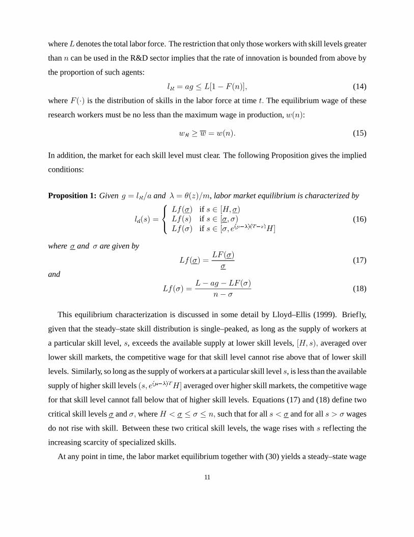
In addition, the market for each skill level must clear. The following Proposition gives the implied

conditions:

Proposition 1: Given � � ���� and � � ������, labor market equilibrium is characterized by

����� �

��

"!�#� if � � ���#�"!��� if � � �#� #�"!�#� if � � �#� ������ �����

(16)

where# and # are given by

"!�#� �" �#�

#(17)

and

"!�#� �"� �� � " �#�

�� #(18)

This equilibrium characterization is discussed in some detail by Lloyd–Ellis (1999). Briefly,

given that the steady–state skill distribution is single–peaked, as long as the supply of workers at

a particular skill level,�, exceeds the available supply at lower skill levels,��� ��� averaged over

lower skill markets, the competitive wage for that skill level cannot rise above that of lower skill

levels. Similarly, so long as the supply of workers at a particular skill level�, is less than the available

supply of higher skill levels��� ����� �� averaged over higher skill markets, the competitive wage

for that skill level cannot fall below that of higher skill levels. Equations (17) and (18) define two

critical skill levels# and#� where� � # � # � �� such that for all� � # and for all� � # wages

do not rise with skill. Between these two critical skill levels, the wage rises with� reflecting the

increasing scarcity of specialized skills.

At any point in time, the labor market equilibrium together with (30) yields a steady–state wage

11

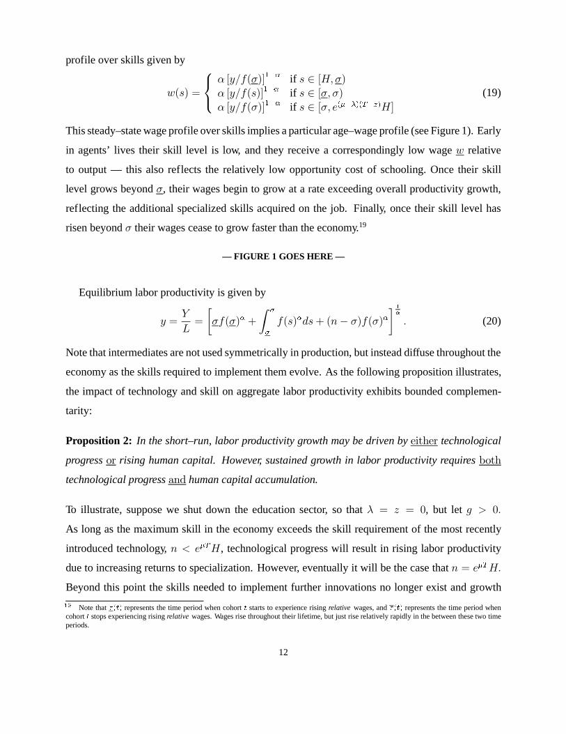
profile over skills given by

��� �

��

�$�!�#����� if � � ���#�

�$�!������� if � � �#� #�

�$�!�#����� if � � �#� ������ �����

(19)

This steady–state wage profile over skills implies a particular age–wage profile (see Figure 1). Early

in agents’ lives their skill level is low, and they receive a correspondingly low wage relative

to output — this also reflects the relatively low opportunity cost of schooling. Once their skill

level grows beyond#, their wages begin to grow at a rate exceeding overall productivity growth,

reflecting the additional specialized skills acquired on the job. Finally, once their skill level has

risen beyond# their wages cease to grow faster than the economy.19

— FIGURE 1 GOES HERE —

Equilibrium labor productivity is given by

$ ��

"�

#!�#��

� �

�

!����� ��� #�!�#��� ��

� (20)

Note that intermediates are not used symmetrically in production, but instead diffuse throughout the

economy as the skills required to implement them evolve. As the following proposition illustrates,

the impact of technology and skill on aggregate labor productivity exhibits bounded complemen-

tarity:

Proposition 2: In the short–run, labor productivity growth may be driven by������ technological

progress�� rising human capital. However, sustained growth in labor productivity requires����

technological progress� human capital accumulation.

To illustrate, suppose we shut down the education sector, so that� � � � �, but let � � ��

As long as the maximum skill in the economy exceeds the skill requirement of the most recently

introduced technology,� � � �, technological progress will result in rising labor productivity

due to increasing returns to specialization. However, eventually it will be the case that� � � ��

Beyond this point the skills needed to implement further innovations no longer exist and growth

� Note that���� represents the time period when cohort� starts to experience risingrelative wages, and���� represents the time period whencohort� stops experiencing risingrelative wages. Wages rise throughout their lifetime, but just rise relatively rapidly in the between these two timeperiods.

12

must cease. Conversely, suppose we shut down the R&D sector so that� � �, but let� � �. In this

case, skill accumulation may raise labor productivity by allowing a more efficient usage of existing

intermediate technologies in final production. However, as� grows relative to�� it will eventually

be the case that the skill–constraints on the use of intermediates in final production no longer bind,

and their marginal products are equalized.20 Beyond this point, production efficiency cannot be

improved any further and growth must cease.

3. Endogenous Growth

In this section, we embed the production structure described in Section 2 in a dynamic general

equilibrium model of endogenous growth. In particular, we characterize the balanced growth paths

that arise when labour is allocated optimally across activities. In Section 4, we illustrate the impli-

cations of this model for the effectiveness of growth–promoting policies and the interpretation of

recent empirical analyses of growth.

3.1 Intertemporal Optimization

We consider a closed economy in which households have identical preferences over a single final

good given by the discounted flow

%��� �

��

�

�������� � � &�'�'� (21)

where( � ��� �� is the rate of pure time preference and&�'� is their time' consumption. The

final good is the numeraire. As described above, each household is composed of an infinite stream

of continuously overlapping generations. Households can borrow or lend freely at the equilibrium

instantaneous interest rate)�'�, there is no utility of leisure and children do not inherit the human

capital of their parents. It follows that although consumption and schooling decisions are made by

the household, we can break the optimization problem down into two steps.

First, household member* chooses the length of time in school,�, so as to maximize his/her

contribution to household wealth. The resulting lifetime wealth of the*th successor of the current

� With rising intermediate productivity, the efficient allocation of intermediates requires that price differences reflect only productivity differences(see Section 5).

13

household member is given by

+ �*� � ����

� �����

���

���������� ��� �*� '�' (22)

where,�'� �� �

�)�-�- represents the discount factor, �*� '� is the time' wage rate of the current

household member’s*th successor. A second–order condition must also hold (see below).

Second, a household whose current member was born at time� � �maximizes utility (21) subject

to the intertemporal budget constraint:��

�

�������������&�'�' �

�

�

������������� ��� '�' �����

���� ��+ �*� .��� (23)

where.��� is the current value of the household’s assets and������ ����.��� � ��

Household assets consist of claims to the profits streams of intermediate firms. The value of

claims to the profits of intermediate producers in industry� using technology�, �/��� �� '�����, is

0 ��� �� �� �

��

�

�������������/��� �� '�'� (24)

The reward to investment in R&D is a claim, with value0 ��� ��, to the profits of intermediate firms

that use the technology. From (32), the labor used to produce one new technology (����� � �) is

������ and each unit of labor costs �. With free entry into the sector, the equilibrium value of this

claim must equal the cost of innovation:

0 ��� � ��

�� (25)

3.2 General Equilibrium

Given initial stocks of transferrable skill,����, and frontier knowledge,����, acompetitive equi-

librium for this economy satisfies the following conditions:

� Final goods producers choose intermediates to maximize profits, (2).

� Intermediate producers set prices and hire labor so as to maximize profits, (3) and (4).

� Workers allocate themselves to the labor market which offers the highest wage for their skill.

� Households choose the optimal amount of schooling for each cohort, (22).

� Households allocate consumption over time so as to maximize (21), subject to (22) and (23).

With time separable log–utility and perfect capital markets, the consumption of each household,

14

and therefore aggregate consumption,1, optimally grows at the instantaneous rate:

�1

1�

�&

&� ) � (� (26)

� Firms in the R&D sector earn zero profits, (25).

� The final goods market clears. Since the final good is the numeraire and the economy is closed,

this implies that

1��� � � ���� (27)

� The asset market clears. Differentiating (24) with respect to time yields the no arbitrage condition,

which requires that the rate of return on all firm shares must equal the rate of interest (see Grossman

and Helpman, 1991). In particular, for the most recently introduced intermediate,

/���

0 ���

�0 ���

0 ���� )� (28)

where/��� is the total profit of intermediate firms using the most recently introduced technology,

�.21

� The labor market clears: (13), (14) and (15) hold, and the market for each skill–level clears.

3.3 Stationary Growth Paths

We now characterize the stationary competitive growth paths for this economy. Along such a path

the distribution of skills is given by (11), and the individual labor market clearing conditions are

given by (16), (17) and (18).22 A key variable in our analysis is an index of ‘‘labor market tightness’’

given by

2 ��

�

�

��� �����

�#

#

���

�

�

��� �����

�

� ����

� (29)

The variable2 measures the impact of the steady–state labor market equilibrium on the incentives

both to invest in education and to invest in R&D. The first term is the portion of time each cohort

spends in school and the second term reflects the growth rate in the wages during a worker’s lifetime.

The larger is2 the greater is the incentive for individual households to invest in education. This

is because (a) the more time individuals spend in school the fewer low-skilled workers in the labor

�� Note that it must be the case in equilibrium that���� � ������������������ This distribution of skills and the associated labor market equilibrium conditions are correctonly along a stationary growth path.

15

force and the greater the returns to scarce skills, and (b) the greater is the growth in wages the higher

are the net returns from education. In contrast, the larger is2 the less incentive firms have to invest

in R&D. This is because (a) the more time individuals spend in school, the smaller is the labor force

and, hence, the lower is the size of the market, and (b) the greater is the relative cost of skilled labor,

the lower are the net profits from innovation. Note that increased on the job learning� raises the

opportunity costs of schooling, but slackens the constraints associated with skill, thereby reducing

the opportunity cost of research.

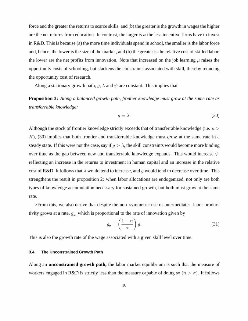
Along a stationary growth path,�, � and2 are constant. This implies that

Proposition 3: Along a balanced growth path, frontier knowledge must grow at the same rate as

transferrable knowledge:

� � �� (30)

Although the stock of frontier knowledge strictly exceeds that of transferrable knowledge (i.e.� �

�), (30) implies that both frontier and transferrable knowledge mustgrow at the same rate in a

steady state. If this were not the case, say if� � �, the skill constraints would become more binding

over time as the gap between new and transferrable knowledge expands. This would increase2,

reflecting an increase in the returns to investment in human capital and an increase in the relative

cost of R&D. It follows that�would tend to increase, and� would tend to decrease over time. This

strengthens the result in proposition 2: when labor allocations are endogenized, not only are both

types of knowledge accumulation necessary for sustained growth, but both must grow at the same

rate.

>From this, we also derive that despite the non–symmetric use of intermediates, labor produc-

tivity grows at a rate,��, which is proportional to the rate of innovation given by

�� �

���

��� (31)

This is also the growth rate of the wage associated with a given skill level over time.

3.4 The Unconstrained Growth Path

Along anunconstrained growth path, the labor market equilibrium is such that the measure of

workers engaged in R&D is strictly less than the measure capable of doing so�� � #�. It follows

16

that (15) holds with a strict inequality. This also implies that the wage in research will be exactly

equal to the highest wage in production ( � � �#��. The unshaded area34� in Figure 2

illustrates the combinations of� and2 that are consistent with such a labor market equilibrium.

Correspondingly, the boundary4� represents combinations of� and2 which yield a labor market

equilibria in which all workers who are capable of working in the R&D sector are doing so (� � #).

This boundary is described by

2 � ����

���

�

��� ���� (32)

Along this4� boundary, high growth is associated with low values of2 because high rates of

innovation can only be sustained by high levels of education that serve to compress the dispersion

of skills.

Combining (4), (13), (25), (26), (27), (28) and (31) yields the stationary combinations of� and

2 such that the expected benefits from the marginal innovation are just equal to the labor costs of

R&D, and equilibrium in the labor market obtains. This is given by

2 � ����

���

��( ��

��� ���� (33)

and is depicted as the,5 curve in Figure 2. One can interpret the,5 curve as being analogous

to a relative demand curve forgrowth in new skills. The schedule is downward sloping reflecting

the fact that, in equilibrium, investment in R&D,�, depends negatively on the cost of skilled labor

relative to that used in production, which is reflected by2. Given2� the rate of innovation depends

positively on the productivity of R&D labor,���, and the size of the population,���23 An increase

in either of these variables will cause the,5 schedule to shift up and to the right. Note that if

2 � �, implying no wage dispersion in production and no education sector, this equation would be

identical to that in Grossman and Helpman (1991, p. 61).

Solving (22), and using (26) and (31), yields the household’s optimal schooling condition in

steady state:

� � 2� ��

(� ��� ���� ����

���� � �

��� � �� ��

���

�

���� ��� ��

��� (34)

�� Note however that the model can easily be adapted to allow for population growth (see Section 5).

17

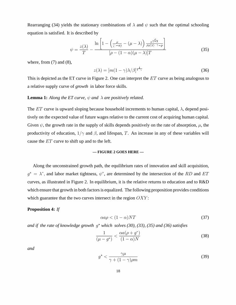
Rearranging (34) yields the stationary combinations of� and2 such that the optimal schooling

equation is satisfied. It is described by

2 �����

��

��

��

��

������ ��� ��

��

����

��������

��(� ��� ���� ����

(35)

where, from (7) and (8),

���� � ����� �������

��� (36)

This is depicted as the ET curve in Figure 2. One can interpret the6� curve as being analogous to

a relative supply curve ofgrowth in labor force skills.

Lemma 1: Along the ET curve,2 and � are positively related.

The6� curve is upward sloping because household increments to human capital,�, depend posi-

tively on the expected value of future wages relative to the current cost of acquiring human capital.

Given2, the growth rate in the supply of skills depends positively on the rate of absorption,�, the

productivity of education,��� and�, and lifespan,� . An increase in any of these variables will

cause the6� curve to shift up and to the left.

— FIGURE 2 GOES HERE —

Along the unconstrained growth path, the equilibrium rates of innovation and skill acquisition,

�� � ��� and labor market tightness,2�, are determined by the intersection of the,5 and6�

curves, as illustrated in Figure 2. In equilibrium, it is the relative returns to education and to R&D

which ensure that growth in both factors is equalized. The following proposition provides conditions

which guarantee that the two curves intersect in the region34� :

Proposition 4: If

�( � ��� ��� (37)

and if the rate of knowledge growth�� which solves (30), (33), (35) and (36) satisfies

�

��� ������( ���

��� ��(38)

and

�� ���

� ��� ��(�(39)

18

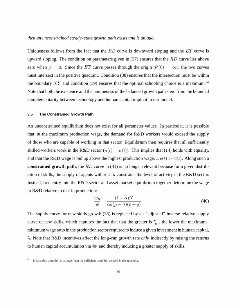
then an unconstrained steady–state growth path exists and is unique.

Uniqueness follows from the fact that the,5 curve is downward sloping and the6� curve is

upward sloping. The condition on parameters given in (37) ensures that the,5 curve lies above

zero when� � �. Since the6� curve passes through the origin (����� � �), the two curves

must intersect in the positive quadrant. Condition (38) ensures that the intersection must be within

the boundary4� and condition (39) ensures that the optimal schooling choice is a maximum.24

Note that both the existence and the uniqueness of the balanced growth path stem from the bounded

complementarity between technology and human capital implicit in our model.

3.5 The Constrained Growth Path

An unconstrained equilibrium does not exist for all parameter values. In particular, it is possible

that, at the maximum production wage, the demand for R&D workers would exceed the supply

of those who are capable of working in that sector. Equilibrium then requires that all sufficiently

skilled workers work in the R&D sector (���� � #���). This implies that (14) holds with equality,

and that the R&D wage is bid up above the highest production wage, ���� � ���. Along such a

constrained growth path, the,5 curve in (33) is no longer relevant because for a given distrib-

ution of skills, the supply of agents with� � � constrains the level of activity in the R&D sector.

Instead, free entry into the R&D sector and asset market equilibrium together determine the wage

in R&D relative to that in production:

�

�

��� ��

���� ���( ��� (40)

The supply curve for new skills growth (35) is replaced by an ‘‘adjusted’’ inverse relative supply

curve of new skills, which captures the fact that that the greater is��

�, the lower the maximum–

minimum wage ratio in the production sector required to induce a given investment in human capital,

�. Note that R&D incentives affect the long–run growth rateonly indirectly by raising the returns

to human capital accumulation via���

and thereby inducing a greater supply of skills.

�� In fact, this condition is stronger than the sufficient condition derived in the appendix.

19

4. Implications

In this section, we highlight some of the implications of our model. Since our growth process nests

those implied by other models, many standard results in the growth literature also apply here, at least

qualitatively. Consequently, we focus only on implications that are specific to our framework. Not

surprisingly, in contrast to models with a single primary engine of growth, factors that affect both

R&D and human capital accumulation have effects on growth. However, the nature of these growth

effects reflect the crucial role of bounded complementarity within our model. In order for a factor

to increase growth, it must not only increase the rate of accumulation of one type of knowledge, but

also induce an accompanying increase in the accumulation of the other type of knowledge. Without

this induced response, higher growth could not be sustained. If, however, that were this comple-

mentarity not bounded, growth would be explosive. More precisely, factors which directly stimulate

innovation (e.g. R&D productivity,���) raise the returns to investment in education, which induces

the necessary supporting increase in education. Similarly, factors which directly stimulate increased

investment in education (e.g. the quality of education,�) raise the returns to investment in R&D,

thereby inducing the expansion of technology that gives the additional human capital value.

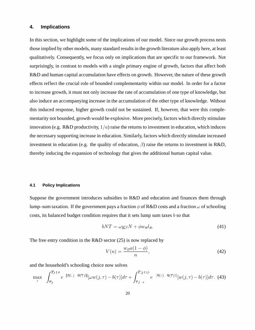
4.1 Policy Implications

Suppose the government introduces subsidies to R&D and education and finances them through

lump–sum taxation. If the government pays a fraction7 of R&D costs and a fraction8 of schooling

costs, its balanced budget condition requires that it sets lump sum taxes9 so that

9�� � 8 �� 7 ���� (41)

The free entry condition in the R&D sector (25) is now replaced by

0 ��� � ����� 7�

�� (42)

and the household’s schooling choice now solves

����

� ���

�

���������� ����8 �*� '�� 9�'��'

� �����

���

���������� ���� �*� '�� 9�'��' � (43)

20

Proceeding as before yields the following equilibrium relationships:

2 � ����

���

����� 7��( ��

��� ���

�(44)

2 �����

��

�����

��

������ ��� ��

�����

��������

��

�

���

��(� ��� ���� ����

(45)

Growth responds positively to both types of subsidy. However, the fact that both technological

change and human capital accumulation are necessary for growth means that, although the menu

of possible policy instruments is expanded, the effectiveness of any individual instrument used in

isolation is diminished:

Proposition 5:

(a) The long–run effectiveness of R&D subsidies is constrained by the responsiveness of education

to the growth in demand for skills.

(b) The long–run effectiveness of education subsidies is constrained by the responsiveness of R&D

to the growth in supply of skills.

These implications can be understood using Figure 3. In the left panel, an R&D subsidy causes

the,5 curve to shift to the right. In the standard innovation–based growth model, the6� curve

would be horizontal, reflecting the perfect technological mobility of labor. The effect of the subsidy

on growth would be to increase it from�� to ��. However, in our model, absorptive capacity on the

job is bounded, so that a long–run increase in growth can only be supported if human capital growth

also rises. This is accomplished by the endogenous rise in the relative returns to schooling, but since

this also raises the relative costs of R&D, the increase in growth is partially offset and the actual

long–run growth rate increases only as far as��.

Conversely, in the right panel, a subsidy to education causes the ET curve to shift to the right.

In a human capital–based growth model, the,5 curve would be horizontal, reflecting the costless

introduction of technology. The effect of the subsidy would be to increase growth from��� to ���.

However, in our model the increase in productivity that can be obtained by increasing human capital

on a given set of technologies is bounded, so that a long–run increase in growth can only be sustained

if new technologies are developed and adopted. This is accomplished by the endogenous increase in

21

the relative return to R&D, but since this also reduces the relative returns to schooling, the increase

in growth is partially offset and the growth rate increase only as far as���.

— FIGURE 3 GOES HERE —

4.2 The Empirical Link between Schooling and Growth

The expression for optimal schooling (34) is similar to that derived by Bils and Klenow (1999,

equation 16). This should not be surprising given that they are both based on the same Mincerian

model of schooling. However, there are some important differences. Theirs is a partial equilibrium

analysis, with a fixed interest rate, in which expected productivity growth enters through its effect on

discounting. In our general equilibrium analysis, under the assumption of log preferences, this effect

is not present because the interest rate fully adjusts in response to high consumption growth:) �

�� � (. As a consequence, productivity growth affects schooling through its equilibrium impact on

incentives via labor market tightness,2. Technological change affects schooling decisions not only

through the valuation of future wages via discounting, but also through affecting wages and returns

to education directly.25 This more direct effect of technological change on educational investments

is a consequence of bounded complementarity between education and technology.

The relationship between schooling and growth in our model also differs from that discussed by

Bils and Klenow for other reasons. First, in our basic model, wages rise with skill only because

higher skills are increasingly scarce.26 This implies an obsolescence effect whereby an individual’s

wage growth depends on the rate at which he/she learnsrelative to the growth in the human capital

of the most recent graduates�� � ��. Second, firms have monopoly power so that households do

not appropriate the full static returns from their investments ( � �). Finally, individuals’ wages

grow relative to GDP for only a portion of an individual’s lifetime (2 � �).

4.3 The Catch–Up Effect

Nelson and Phelps (1966) posit that human capital accumulates faster, the further it is behind the

technological frontier. Jones (1999) captures this idea in a reduced form way in accounting for

�� In our model, we could allow for both effects by assuming CES preferences, in which case� � � � �� ��� �� � .�� When intermediate productivity rises with skill, wages also depend on own human capital.

22

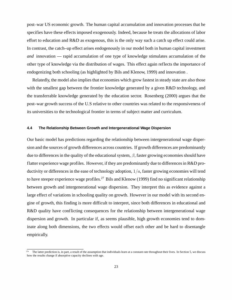
post–war US economic growth. The human capital accumulation and innovation processes that he

specifies have these effects imposed exogenously. Indeed, because he treats the allocations of labor

effort to education and R&D as exogenous, this is the only way such a catch up effect could arise.

In contrast, the catch–up effect arises endogenously in our model both in human capital investment

and innovation — rapid accumulation of one type of knowledge stimulates accumulation of the

other type of knowledge via the distribution of wages. This effect again reflects the importance of

endogenizing both schooling (as highlighted by Bils and Klenow, 1999) and innovation .

Relatedly, the model also implies that economies which grow fastest in steady state are also those

with the smallest gap between the frontier knowledge generated by a given R&D technology, and

the transferrable knowledge generated by the education sector. Rosenberg (2000) argues that the

post–war growth success of the U.S relative to other countries was related to the responsiveness of

its universities to the technological frontier in terms of subject matter and curriculum.

4.4 The Relationship Between Growth and Intergenerational Wage Dispersion

Our basic model has predictions regarding the relationship between intergenerational wage disper-

sion and the sources of growth differences across countries. If growth differences are predominantly

due to differences in the quality of the educational system,�, faster growing economies should have

flatter experience wage profiles. However, if they are predominantly due to differences in R&D pro-

ductivity or differences in the ease of technology adoption,���, faster growing economies will tend

to have steeper experience wage profiles.27 Bils and Klenow (1999) find no significant relationship

between growth and intergenerational wage dispersion. They interpret this as evidence against a

large effect of variations in schooling quality on growth. However in our model with its second en-

gine of growth, this finding is more difficult to interpret, since both differences in educational and

R&D quality have conflicting consequences for the relationship between intergenerational wage

dispersion and growth. In particular if, as seems plausible, high growth economies tend to dom-

inate along both dimensions, the two effects would offset each other and be hard to disentangle

empirically.

�� The latter prediction is, in part, a result of the assumption that individuals learn at a constant rate throughout their lives. In Section 5, we discusshow the results change if absorptive capacity declines with age.

23

4.5 The Role of Lifespan

Heckman and Klenow (1997) and Bils and Klenow (1999) argue that longer lifespan stimulates

educational investment because it implies a longer time over which to reap the benefits. In our

model, lifespan also has another general equilibrium effect — it generates a scale effect, raising the

innovation rate and the returns to education. Increased lifespan increases the amount of knowledge

that can be learned on the job. This additional skill accumulation increases the supply of skilled

workers, depresses the cost of innovation, and ultimately speeds up growth. Although, with zero

population growth, the effect of lifespan cannot be distinguished from the overall scale effect, when

we adapt the model so as to mitigate the scale effect and allow for population growth, the distinct

effect of lifespan becomes clear (see Section 5).

5. Extensions to the Basic Model

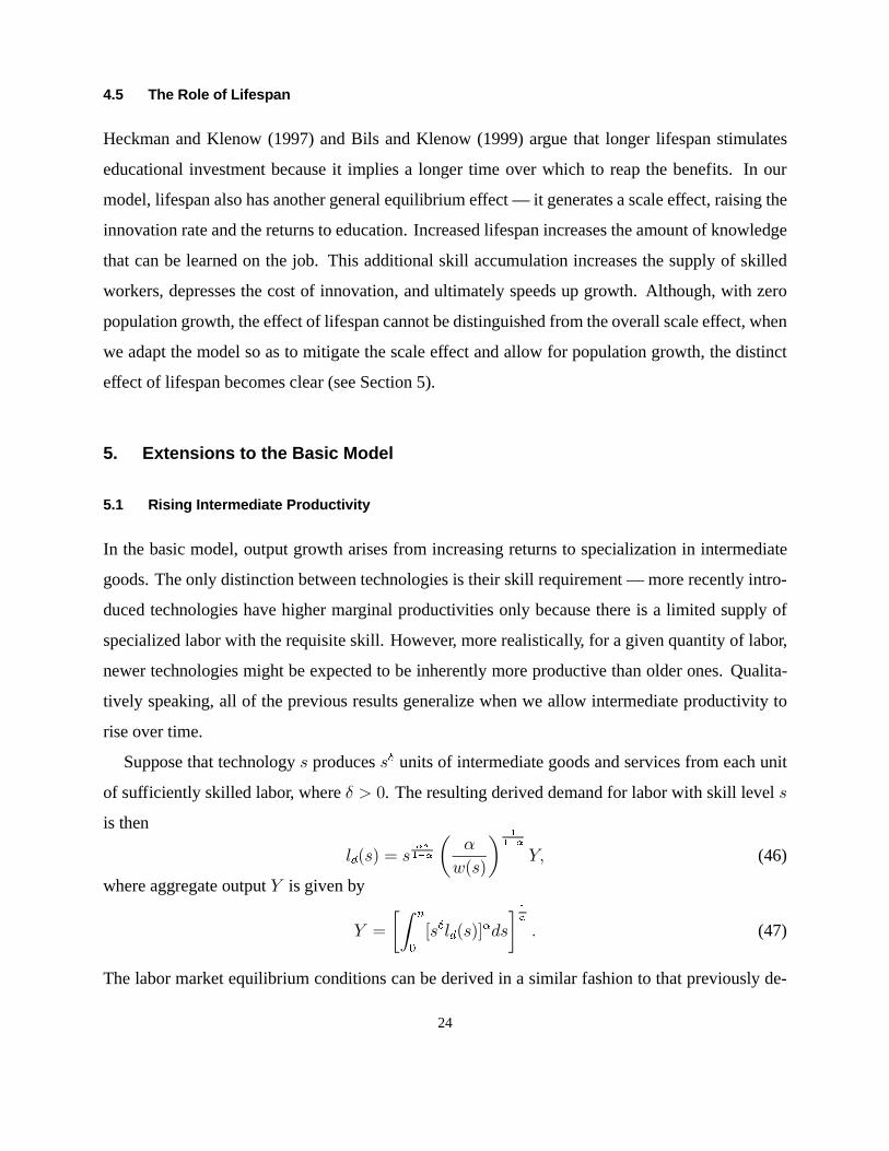
5.1 Rising Intermediate Productivity

In the basic model, output growth arises from increasing returns to specialization in intermediate

goods. The only distinction between technologies is their skill requirement — more recently intro-

duced technologies have higher marginal productivities only because there is a limited supply of

specialized labor with the requisite skill. However, more realistically, for a given quantity of labor,

newer technologies might be expected to be inherently more productive than older ones. Qualita-

tively speaking, all of the previous results generalize when we allow intermediate productivity to

rise over time.

Suppose that technology� produces�� units of intermediate goods and services from each unit

of sufficiently skilled labor, where: � �. The resulting derived demand for labor with skill level�

is then

����� � �����

�

���

� ����

�� (46)

where aggregate output� is given by

� �

� �

�

�����������

� ��

� (47)

The labor market equilibrium conditions can be derived in a similar fashion to that previously de-

24

scribed, by simply re–formulating the arguments in terms of ‘‘productivity–adjusted’’ demand for

labor with skill�:

����� ������

�����

�

�

���

� ����

�� (48)

For low skill levels, the demand for labor from intermediates using the associated technology, com-

pletely exhausts the available supply without driving the wage above that earned by higher–skilled

workers. However, there exists a skill level# above which the productivity adjusted supply of labor

with skill index�, !��������� is less than the productivity–adjusted supply of labor with skills��� ;�

divided equally across technologies,�#� ��. It follows that, in equilibrium, an equal productivity–

adjusted quantity of labor is allocated to each technology� � �#� ��, and that the actual quantity

of labor using technology� must be� ���

����!�#�. Since this exceeds!���, the remainder is drawn

from the pool of workers with skills greater than� that are not being used in the R&D sector,

�� ���� ���". Labor market equilibrium is therefore characterized by

����� �

����

" �

�

� ����!�#�� if � � ���#�

"!���� if � � �#� #�

" �

�

� ����!�#�� if � � �#� ������ �����

(49)

where � �

�

��

#

����� !�#�

�� � �#�� (50)

and � �

�

�� �#

�����!�#�

��

��

"� �� �#�� (51)

The associated wage profile is qualitatively similar to (13), except that the elasticity of the wage

with respect to skills� � �#� #� is now��� � :.

The balanced growth path with rising intermediate productivity satisfies (30) the following sys-

tem of equations

2 � ����

���

��( ��

��� :���(52)

2 �����

��

��

�� �

����� ���

��� � �������

�

�

������� ��� ��

���(� ��� :���� ����

(53)

25

�� �

���

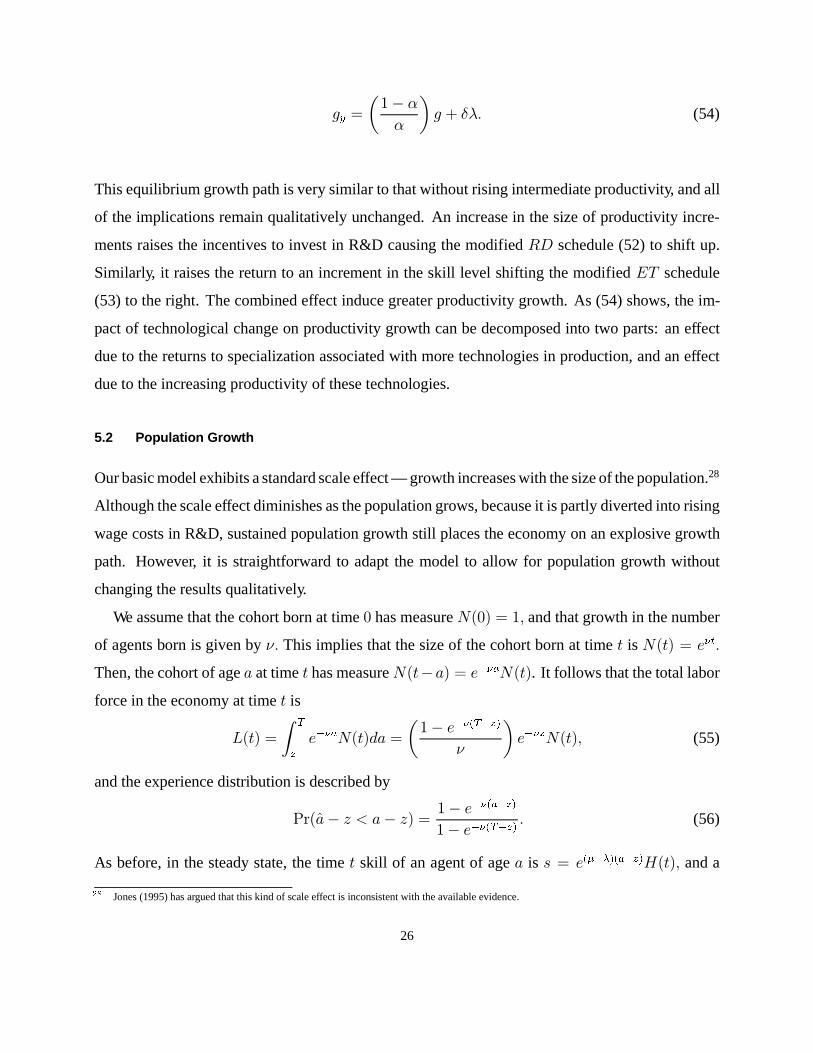
�� :�� (54)

This equilibrium growth path is very similar to that without rising intermediate productivity, and all

of the implications remain qualitatively unchanged. An increase in the size of productivity incre-

ments raises the incentives to invest in R&D causing the modified,5 schedule (52) to shift up.

Similarly, it raises the return to an increment in the skill level shifting the modified6� schedule

(53) to the right. The combined effect induce greater productivity growth. As (54) shows, the im-

pact of technological change on productivity growth can be decomposed into two parts: an effect

due to the returns to specialization associated with more technologies in production, and an effect

due to the increasing productivity of these technologies.

5.2 Population Growth

Our basic model exhibits a standard scale effect — growth increases with the size of the population.28

Although the scale effect diminishes as the population grows, because it is partly diverted into rising

wage costs in R&D, sustained population growth still places the economy on an explosive growth

path. However, it is straightforward to adapt the model to allow for population growth without

changing the results qualitatively.

We assume that the cohort born at time� has measure���� � �� and that growth in the number

of agents born is given by-� This implies that the size of the cohort born at time� is���� � ����

Then, the cohort of age� at time� has measure������ � ��������. It follows that the total labor

force in the economy at time� is

"��� �

�

�

��������� �

��� ���� ���

-

���������� (55)

and the experience distribution is described by

������ � � �� �� ��� ��������

�� ���� ���� (56)

As before, in the steady state, the time� skill of an agent of age� is � � ��������������� and a

�� Jones (1995) has argued that this kind of scale effect is inconsistent with the available evidence.

26

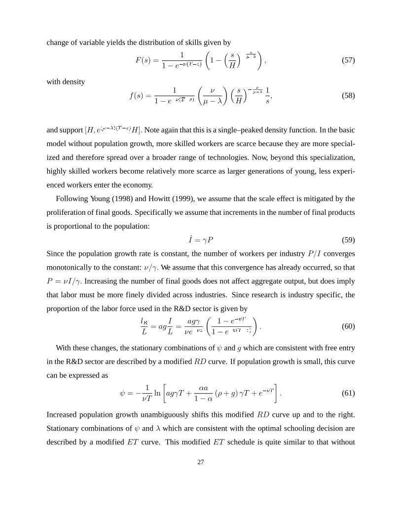
change of variable yields the distribution of skills given by

��� ��

�� ���� ���

���

� ��

��

����

�� (57)

with density

!��� ��

�� ���� ���

�-

�� �

�� ��

��

���� �

�� (58)

and support��� ������ ������Note again that this is a single–peaked density function. In the basic

model without population growth, more skilled workers are scarce because they are more special-

ized and therefore spread over a broader range of technologies. Now, beyond this specialization,

highly skilled workers become relatively more scarce as larger generations of young, less experi-

enced workers enter the economy.

Following Young (1998) and Howitt (1999), we assume that the scale effect is mitigated by the

proliferation of final goods. Specifically we assume that increments in the number of final products

is proportional to the population:

�� � �< (59)

Since the population growth rate is constant, the number of workers per industry<�� converges

monotonically to the constant:-��� We assume that this convergence has already occurred, so that

< � -���� Increasing the number of final goods does not affect aggregate output, but does imply

that labor must be more finely divided across industries. Since research is industry specific, the

proportion of the labor force used in the R&D sector is given by

��"

� ���

"�

���

-����

��� ��

�� �� � ���

�� (60)

With these changes, the stationary combinations of2 and� which are consistent with free entry

in the R&D sector are described by a modified,5 curve. If population growth is small, this curve

can be expressed as

2 � ��

-���

����

�

�� �( �� �� ���

�� (61)

Increased population growth unambiguously shifts this modified,5 curve up and to the right.

Stationary combinations of2 and� which are consistent with the optimal schooling decision are

described by a modified6� curve. This modified6� schedule is quite similar to that without

27

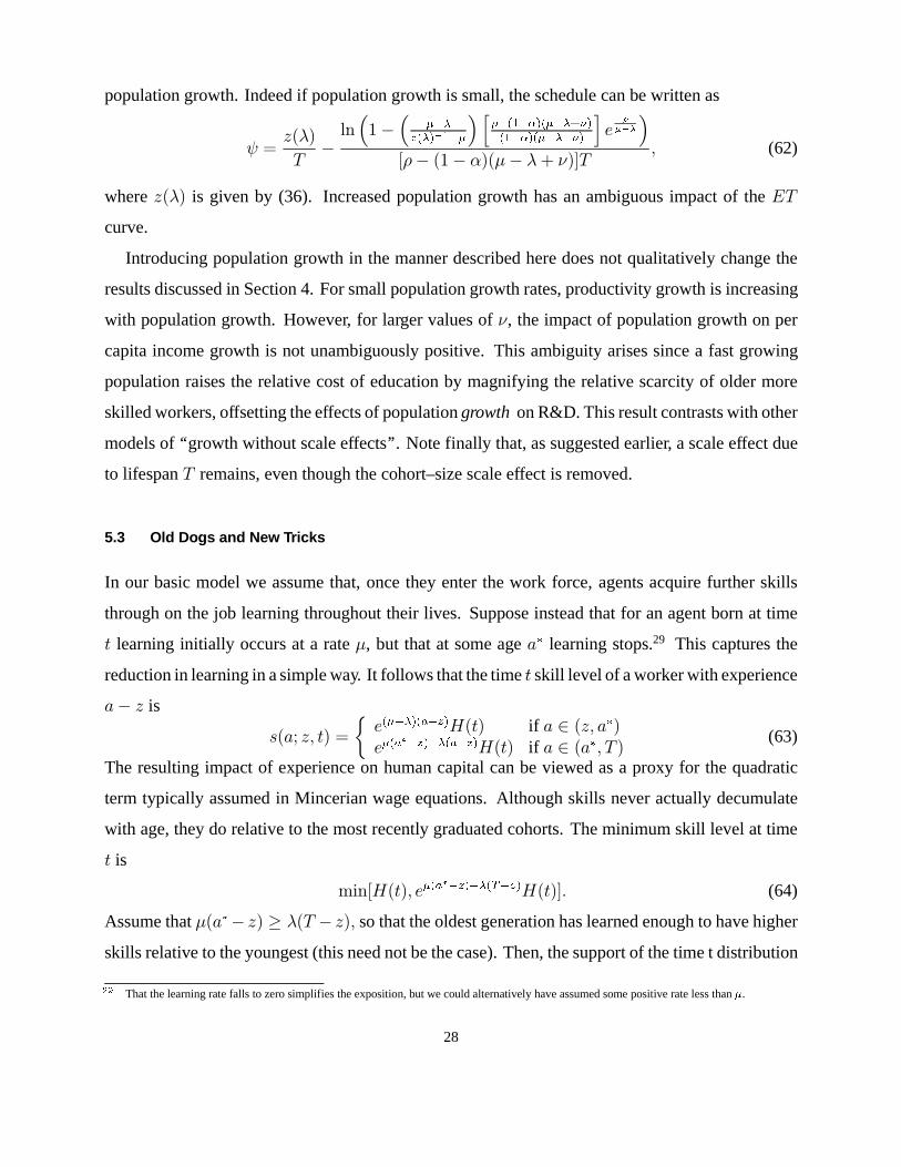
population growth. Indeed if population growth is small, the schedule can be written as

2 �����

��

�����

���

�������

� ��������������

�����������

��

�

���

��(� ��� ���� � -���

� (62)

where���� is given by (36). Increased population growth has an ambiguous impact of the6�

curve.

Introducing population growth in the manner described here does not qualitatively change the

results discussed in Section 4. For small population growth rates, productivity growth is increasing

with population growth. However, for larger values of-, the impact of population growth on per

capita income growth is not unambiguously positive. This ambiguity arises since a fast growing

population raises the relative cost of education by magnifying the relative scarcity of older more

skilled workers, offsetting the effects of populationgrowth on R&D. This result contrasts with other

models of ‘‘growth without scale effects’’. Note finally that, as suggested earlier, a scale effect due

to lifespan� remains, even though the cohort–size scale effect is removed.

5.3 Old Dogs and New Tricks

In our basic model we assume that, once they enter the work force, agents acquire further skills

through on the job learning throughout their lives. Suppose instead that for an agent born at time

� learning initially occurs at a rate�, but that at some age�� learning stops.29 This captures the

reduction in learning in a simple way. It follows that the time� skill level of a worker with experience

�� � is

��� �� �� �

��������������� if � � ��� ������

��������������� if � � ���� � �

(63)

The resulting impact of experience on human capital can be viewed as a proxy for the quadratic

term typically assumed in Mincerian wage equations. Although skills never actually decumulate

with age, they do relative to the most recently graduated cohorts. The minimum skill level at time

� is

��������� ���������� ��������� (64)

Assume that����� �� � ��� � ��� so that the oldest generation has learned enough to have higher

skills relative to the youngest (this need not be the case). Then, the support of the time t distribution

� That the learning rate falls to zero simplifies the exposition, but we could alternatively have assumed some positive rate less than.

28

of skills is ������ ���������������� and the distribution of skills is

��� �

��

�

����� ������

�

����

�if � � ���

������� �������

������ ������

�����

� �� ������

�� ���otherwise

(65)

with density

!��� �

��

����� ���

�

�if � � ���

������� �������

������ ���

�

�otherwise

(66)

Note that the distribution of skills remains single–peaked, so that Proposition 1 is still applicable.

In equilibrium, if we looked at a cross–section of ages in a given time period, wages would initially

rise relative to GDP, and then fall with age. In this modified version of the model, R&D investment

incentives are not much altered. Moreover, although an agent’s lifetime wage profile is somewhat

different, so long as on–the–job learning continues for a sufficient time period after graduation,

their basic incentives are not that much altered either.30 Consequently, one can show (see Appendix

B) that an equilibrium growth path which is qualitatively similar to that characterized in Section 3

continues to exist.

6. Concluding Remarks

In this paper, we have constructed a model in which technologies and skills are bounded com-

plements in the determination of the growth process. As a result, growth cannot proceed without

both types of knowledge accumulation, andboth innovation and skill acquisition depend on pri-

vate incentives to make costly investments. Our model captures two important intuitions: that both

the distribution of skills and wages are endogenous, generated by the response of individuals to

the incentives generated by technological change, and that the amount of innovation depends on the

relative scarcity and hence the cost of skill. In addition, to providing a general framework for under-

standing the interactions between technological progress, human capital formation and productivity

growth, our model has unique implications for the effectiveness of growth–enhancing policies, for

the interpretation of the link between growth and schooling, and for other features of the growth

process.

� The analysis is somewhat tedious, but follows the same steps as before. The experience wage profile now consists of 5 parts. Relative to GDP,wages are constant initialy, then grow plateauing at a maximum. After learning stops, the wage then falls relative to GDP, before becoming constantagain.

29

In its most limited sense, our model might be interpreted as a model of a leading–edge devel-

oped economy. Less developed economies do not engage in much frontier R&D, but rather acquire

existing technologies from abroad. Jovanovic (1997) argues that a model of adoption (e.g. Parente,

1994) is a more appropriate characterization for LDCs than innovation–based models of growth.

However, the initial adoption of new technologies is costly.31 That LDC governments are aware

of this is evidenced by the significant allocation of resources towards research extension services

(see Hoff, Braverman and Stiglitz, 1990). In a more general model with international technology

spillovers (along the lines of Howitt, 2000), one could re–interpret our R&D sector as an initial

adoption sector which procures technologies internationally and engages in their costly adoption.

Once the initial adoption costs have been incurred, it becomes possible for the knowledge to dis-

seminate throughout the economy, and eventually to find its way into the education system. This

process exactly parallels the evolution of knowledge explored in this paper.

�� Grossman and Helpman (1991) emphasize that the costs of immitation may often be almost as high as those of innovation.

30

Appendix

Proof of Proposition 3: Substituting for the stationary distribution function into (17) yields

�

��� ��

�

#�

�

#

�

��� ����� #�

��(A1)

# � �� (A2)

Substituting for the stationary distribution function in (18)

�

��� ��

�

#���� � ��� �� � !

������ ��

��� #

(A3)

�

#� � ��� ���� � � � ������ ��

� #�

�(A4)

Combining (A2) and (A4) yields:

�

#� ��� ���� � ���� � ��� ��

�#

#

�(A5)

�

#� ��� ���� � ���� � �2� (A6)

Since in a steady state,� � ���� is constant, and it follows from (A2) that�#�# � �. Along the

steady state growth path the r.h.s. of (A6) is constant so that�#�# � �� From (29), if2 is constant

in the steady state it must be the case that�#�# � �#�# and so� � ��

Growth in Labor Productivity:Integrating over labor demands as follows yields the following ex-

pression for labor productivity

$ ��

"

#

��

��� ��

�

#

��

� �

�

��

��� ��

�

�

��

� ��� #�

��

��� ��

�

#

��� ��

(A7)

$ �#

����

��� ���� � ��

�� �

#�

�

��

��##

����� ��

(A8)

Since along the steady–state growth path both��# and#�# are constant and��� �, it follows that

�� � ���

�

��.

The4� Boundary:If all agents that are available for R&D are being used in that sector, then# � �

and

�� � ��� � ����� ���� � ��� � ����

��� ����� ��

�(A9)

31

Now from (29), noting that# � �and that# � ��, we have

2 ��

�

�

��� ������ �

��

���

�

�

��� ������ ��

��

�

��� ���(A10)

Substituting out �

������ ��

�between (A9) and (A10) and rearranging yields (32).

The,5 Schedule:The maximum wage in production is given by � �#� � �$��� ���� � ��#����.

Hence, it grows at the rate

�

� ��� �

���

�#

#

�� ��� �

����

�� �

��

���

�� � ��� (A11)

Differentiating (25) w.r.t. time therefore yields

�0

0�

�

� � � �� � �� (A12)

The total profit of the most recently introduced intermediate is

/��� �

���

� �

��� ��#� (A13)

Noting that � � and dividing (A13) by (25) yields

/���

0 ����

���� ��

���� ��

��

#� (A14)

Substituting (A12) and (A14) into the no–arbitrage condition (28) then yields���� ��

���� ��

��

#� � � (� (A15)

Substituting for��# using (A6) and rearranging yields (33).

The6� Schedule:The time' equilibrium wage of an agent born at time� is given by

�' � �� �

��

��$�'�#�'����� if ' � �� �� � '�

��$�'���������������

����if ' � �� ' � � '�

��$�'�#�'����� if ' � �� ' � � � �

(A16)

where� � �� � ���� � ��, � � ��� � ��� denotes the dynamic spillover, and' and' are

defined by

������������ � #�� '� � ���#��� (A17)

������������ � #�� '� � ���#��� (A18)

32

The present value of the lifetime steady–state earnings of an agent born at time� is thus given by

+ ��� �� �

�������

�������� �#�'�� '�'

�������

�������� ���'�� '�'

�� ����

�������� �#�'�� '�' (A19)

Substituting using (A16) and differentiating with respect to�, yields

+ ���� �� � ����� �#�� ��� (A20)

��� � ������� ��

�������

���������$�'����������������

����'

� �#����

������� ��� � ������� ��

���������

#���

���� �������

�������������������'

��(A21)

But along the steady–state growth path������ � ��� �� � �������. Hence, the first–order

condition can be written as

��� � ������� ��

�����

#���

����

������������

�������

�������������������' � ����� (A22)

Substituting for#��� using (A2) and integrating yields

��� � ������� �� �������������������������������� � ���������������

���� ���� ��� (

� ����� (A23)

From (A17) we have that, along the steady–state growth path,���������� � �������#��� � ������������.

It follows that

' ��

�� � �� (A24)

From (A18) we have������������� � ���#��� � ���������" ���#��� � ���������" ��������.

Hence,

' ��

�� � 2� (A25)

Substituting (A24) and (A25) into (A23) yields

��� � ������� ������������������

����

�" � � ����������������

������

���� ���� ��� (

� �������������������

(A26)

33

Dividing both sides by������

��� and rearranging yields

��������������" � ��������������� �

���� ���� ��� (

��� � ������� ��

�����������������

�

��� (A27)

Rearranging yields (35).

The Second–order Condition for Optimal Schooling: Differentiating (A21) w.r.t.� yields

+��

�� �� � �#����(���� �#������� ����

���

���������

#���

���� �������

�������������������' (A28)

�#������� �� ������� ���

���������

#���

���� �������

�������������������'

�#������� � ������� ��

���������

#���

���� ���������������

'

�� ���������������

'

�

�

Now from (A17) and (A18) we have����

� ��

��� �������

��� Also we know that��������������� �

��������������� � �����������(��������

�������������������'� It follows that we can write (A28)

as

+��

�� �� � �#����(���� �#������� �

���������

#���

���� �������

�������������������' (A29)

���

��� ��� � ������� ���� ������� ��

������� �

�� �

����� ���� ��� (�

�

Substitution using (A22), allows us to express this as

+��

�� �� � �#��������

�(

���

���

������ � ��� � ������� ���

������� �

�� �

����� ���� ��� (�

�

� �#��������

����

���

������ � (

������� �

�� �

��

� �#����������������

��� � � (

���� � �

�� �

��(A30)

Thus, a sufficient condition for a maximum is

(

���� � �

�� �

��

������

��� � �(A31)

34

This condition will certainly hold if

(

����

�� �

��

������

���(A32)

(

�� ��

�

�����

�

��� ����(A33)

where the last equality follows from (36). Rearranging yields (39).

Proof of Lemma 1:

Case 1:Suppose�� � � �

���. Then, we can write (35) as

2 �����

�

�

��� ���.��� �� ��� .���=����(A34)

where.��� � �

���� � � � � and=��� �

����

�������

��

�

��� � �. Note that.���� � � and

=���� � �. Also observe that existence requires that.���=��� � �. Let

7 � .��� �� ��� .���=���� (A35)

Then7

��

�� ��� .=��

.=

��.=

�.�����

.�

��.==���� � � (A36)

since�� ���.=� � �. Since����� � �, it follows that along the ET curve2�� � ��

Case 2:Suppose�� � � �

���. Then the original expression can be written

2 ����� �.���=���

���� ��� �.���

����

�(A37)

where �.��� � �� �� �

���� �. Note that �.���� � �� Differentiating yields

2

�

����#

��

��� ��

���.=

� �.=� ��

�� �.=

�� �.�����.�

=����

�� �.=�

������

�(A38)

Since����� � � and=���� � �, a sufficient condition for�"��� � is that the term in square brackets

is non–positive. Let� � �.= � �. Then�"

��� � if

� � �� �� ���� �� � � � �� (A39)

Observe first that this holds with equality if� � �. Let� � ���� ������. The ���$

� � ����

�� � � and ���

�$�� �

��$� �. It follows that (A39) must hold with strict inequality for all� � ��

35

Hence, in this case as well2�� � ��

References

Acemoglu, Daron and Joshua Angrist, ‘‘How Large are the Social Returns to Education? Evidence

from Compulsory Schooling Laws,’’NBER Macroeconomic Annual 2000, forthcoming.

Aghion, Philippe and Peter Howitt ‘‘A Model of Growth through Creative Destruction,’’

Econometrica, March 1992, vol. 60 (1), pp. 323–51.

Aghion, Philippe and Peter Howitt,Endogenous Growth Theory,Cambridge, MA: MIT Press,

1998.

Aghion, Philippe and Peter Howitt, ‘‘ ,’’Journal of Economic Growth, 1998.

Arnold, Lutz, ‘‘Endogenous Growth Without Scale Effects: A Comment’’, mimeo, University of

Dortmund, 1999.

Bartel, Ann P and Frank R. Lichtenberg, ‘‘The Comparative Advantage of Educated Workers in

Implementing New Technology,’’Review of Economics and Statistics, 1987, vol. 69, no. 1, pp.

1-11.

Benhabib, Jess and Mark Spiegel, ‘‘The Role of Human Capital in Economic Development:

Evidence from Aggregate Cross Country Date,’’Journal of Monetary Economics,vol. 34, pp.

143-73.

Berman, Eli, John Bound and Zvi Griliches, ‘‘Changes in the Demand for Skilled Labor within

U.S. Manufacturing: Evidence from the Annual Survey of Manufactures,’’Quarterly Journal

of Economics, 1994, vol. 109, no. 2, pp. 367-97.

Bils, Mark and Peter J. Klenow, ‘‘Does Schooling Cause Growth or the Other Way Around?’’

NBER Working Paper No. 6393, 1998.

Caselli, Francesco, ‘‘Technological Revolutions’’,American Economic Review, March 1999, vol.

89, pp. 78–102.

Chari, V. V. and Hugo Hopenhayn, ‘‘Vintage Human Capital, Growth and the Diffusion of New

Technology’’,Journal of Political Economy, 1991, vol. 99, pp. 1142–66.

Eicher, Theo S., ‘‘Interaction between Endogenous Human Capital and Technological Change,’’

The Review of Economic Studies, January 1996, vol. 63 (1), pp. 127–144.

Foster, A.D. and M. Rosenzweig, ‘‘Technical Change and Human Capital Returns and Investments:

Evidence from the Green Revolution,’’ 1996,American Economic Review, 86(4), pp. 931-953.

Galor, Oded and Tsiddon, Daniel, ‘‘Technological Progress, Mobility, and Growth’’,American

Economic Review, June 1997, vol. 87 (3), pp. 363–82.

Galor, Oded and Omer Maov, ‘‘Ability Biased Technological Transition, Wage Inequality and

36

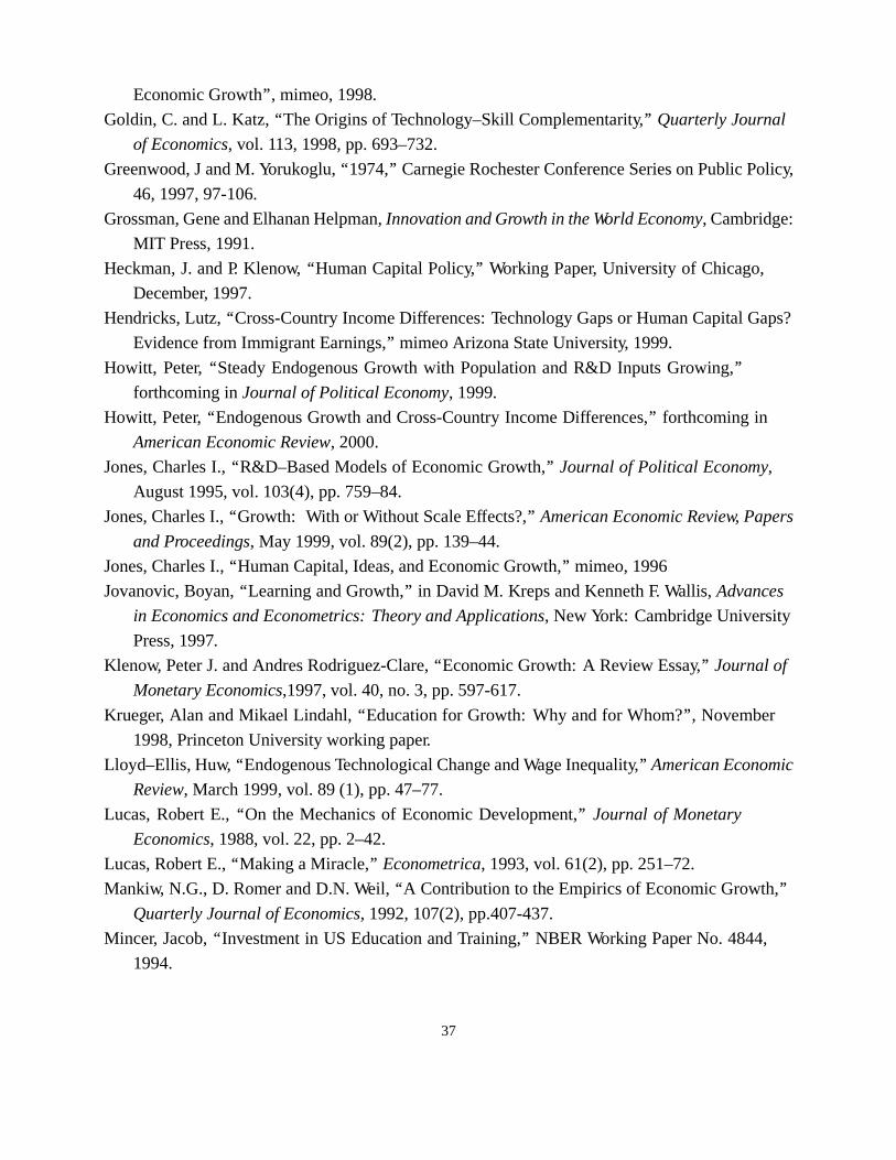
Economic Growth’’, mimeo, 1998.

Goldin, C. and L. Katz, ‘‘The Origins of Technology–Skill Complementarity,’’Quarterly Journal

of Economics, vol. 113, 1998, pp. 693–732.

Greenwood, J and M. Yorukoglu, ‘‘1974,’’ Carnegie Rochester Conference Series on Public Policy,

46, 1997, 97-106.

Grossman, Gene and Elhanan Helpman,Innovation and Growth in the World Economy, Cambridge:

MIT Press, 1991.

Heckman, J. and P. Klenow, ‘‘Human Capital Policy,’’ Working Paper, University of Chicago,

December, 1997.

Hendricks, Lutz, ‘‘Cross-Country Income Differences: Technology Gaps or Human Capital Gaps?

Evidence from Immigrant Earnings,’’ mimeo Arizona State University, 1999.

Howitt, Peter, ‘‘Steady Endogenous Growth with Population and R&D Inputs Growing,’’

forthcoming inJournal of Political Economy, 1999.

Howitt, Peter, ‘‘Endogenous Growth and Cross-Country Income Differences,’’ forthcoming in

American Economic Review, 2000.

Jones, Charles I., ‘‘R&D–Based Models of Economic Growth,’’Journal of Political Economy,

August 1995, vol. 103(4), pp. 759–84.

Jones, Charles I., ‘‘Growth: With or Without Scale Effects?,’’American Economic Review, Papers

and Proceedings, May 1999, vol. 89(2), pp. 139–44.

Jones, Charles I., ‘‘Human Capital, Ideas, and Economic Growth,’’ mimeo, 1996

Jovanovic, Boyan, ‘‘Learning and Growth,’’ in David M. Kreps and Kenneth F. Wallis,Advances

in Economics and Econometrics: Theory and Applications, New York: Cambridge University

Press, 1997.

Klenow, Peter J. and Andres Rodriguez-Clare, ‘‘Economic Growth: A Review Essay,’’Journal of

Monetary Economics,1997, vol. 40, no. 3, pp. 597-617.

Krueger, Alan and Mikael Lindahl, ‘‘Education for Growth: Why and for Whom?’’, November

1998, Princeton University working paper.

Lloyd–Ellis, Huw, ‘‘Endogenous Technological Change and Wage Inequality,’’American Economic

Review, March 1999, vol. 89 (1), pp. 47–77.

Lucas, Robert E., ‘‘On the Mechanics of Economic Development,’’Journal of Monetary

Economics, 1988, vol. 22, pp. 2–42.

Lucas, Robert E., ‘‘Making a Miracle,’’Econometrica, 1993, vol. 61(2), pp. 251–72.

Mankiw, N.G., D. Romer and D.N. Weil, ‘‘A Contribution to the Empirics of Economic Growth,’’

Quarterly Journal of Economics, 1992, 107(2), pp.407-437.

Mincer, Jacob, ‘‘Investment in US Education and Training,’’ NBER Working Paper No. 4844,

1994.

37

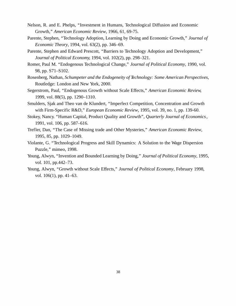
Nelson, R. and E. Phelps, ‘‘Investment in Humans, Technological Diffusion and Economic

Growth,’’ American Economic Review, 1966, 61, 69-75.

Parente, Stephen, ‘‘Technology Adoption, Learning by Doing and Economic Growth,’’Journal of

Economic Theory, 1994, vol. 63(2), pp. 346–69.

Parente, Stephen and Edward Prescott, ‘‘Barriers to Technology Adoption and Development,’’

Journal of Political Economy,1994, vol. 102(2), pp. 298–321.

Romer, Paul M. ‘‘Endogenous Technological Change,’’Journal of Political Economy, 1990, vol.

98, pp. S71–S102.

Rosenberg, Nathan,Schumpeter and the Endogeneity of Technology: Some American Perspectives,

Routledge: London and New York, 2000.

Segerstrom, Paul, ‘‘Endogenous Growth without Scale Effects,’’American Economic Review,

1999, vol. 88(5), pp. 1290–1310.

Smulders, Sjak and Theo van de Klundert, ‘‘Imperfect Competition, Concentration and Growth

with Firm-Specific R&D,’’ European Economic Review, 1995, vol. 39, no. 1, pp. 139-60.

Stokey, Nancy. ‘‘Human Capital, Product Quality and Growth’’,Quarterly Journal of Economics,

1991, vol. 106, pp. 587–616.

Trefler, Dan, ‘‘The Case of Missing trade and Other Mysteries,’’American Economic Review,

1995, 85, pp. 1029–1049.

Violante, G. ‘‘Technological Progress and Skill Dynamics: A Solution to the Wage Dispersion

Puzzle,’’ mimeo, 1998.

Young, Alwyn, ‘‘Invention and Bounded Learning by Doing,’’Journal of Political Economy, 1995,

vol. 101, pp.442–73.

Young, Alwyn, ‘‘Growth without Scale Effects,’’Journal of Political Economy, February 1998,

vol. 106(1), pp. 41–63.

38

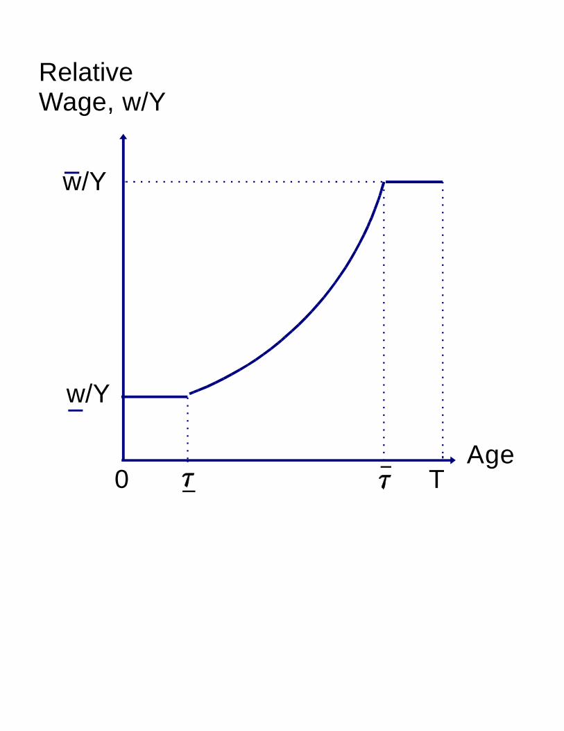
RelativeWage, w/Y

w/Y

w/Y

0 TAge

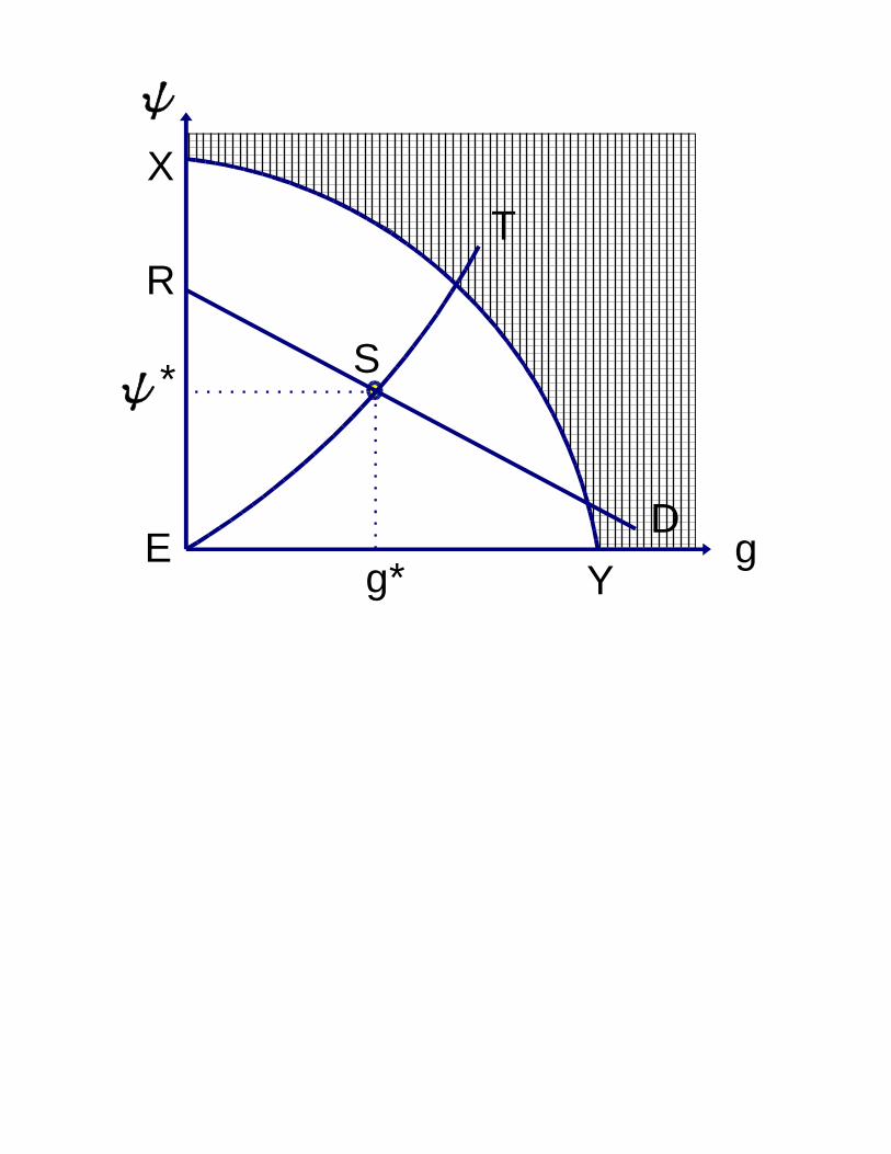
g

S

g*

*

R

DE

T

X

Y

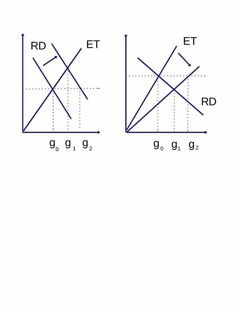
RD ET ET

RD

g g g g g g0 1 2 0 1 2