Twin Deficits: Squaring Theory, Evidence and Common Sense1

Giancarlo Corsetti

European University Institute, University of Rome III and CEPR

and

Gernot J. Müller

Goethe University Frankfurt

This version: March 2006

First Draft: November 2005

Abstract

Appealing to the twin deficit hypothesis, according to which shocks to the government budget move the current account in the same direction, many observers call for fiscal consolidation in the US as a necessary measure to reduce the large external imbalance of this country. We reconsider the international transmission mechanism in a standard two-country two-good business cycle model, and find that fiscal expansions have no effect on the trade balance and thus on the current account i) if the economy is not very open to trade and ii) if fiscal shocks are not too persistent. Under these conditions, the crowding out effect of fiscal shocks on private investment is stronger than conventionally believed. We take this insight to the data and investigate the transmission of fiscal shocks in a VAR model estimated for Australia, Canada, the UK and the US. For the US and Australia, which are less open to trade than Canada and the UK, we find that the external impact of shocks to either government spending or budget deficits is limited, while private investment responds significantly – in line with our theoretical prediction. The reverse is true for Canada and the UK. These results suggest that a fiscal retrenchment in the US may have a limited impact on its current external deficit. However, our results do not weaken the case for fiscal consolidation: by crowding in investment, a fiscal correction will strengthen the ability of the US to generate resources required to service future external liabilities. Keywords: twin deficits, budget deficits, trade deficits, home-bias, openness, crowding out, international transmission of fiscal policy, current account adjustment. JEL classification: E62, E63, F32, F42, H30

1Preliminary version of a paper prepared for the 43rd Panel Meeting of Economic Policy in Vienna. We thank Giuseppe Bertola, four anonymous referees, Keith Küster, Rick van der Ploeg, Morten Ravn, and seminar participants at the European University Institute and Goethe University Frankfurt for helpful comments as well as Larry Schembri for help with the Canadian data. Zeno Enders provided excellent research assistance, Lucia Vigna invaluable help with the text. Corsetti’s work on this project is part of the Pierre Werner Chair Programme on Monetary Union of the Robert Schuman Centre at the European University Institute. Financial support by the programme is gratefully acknowledged. The usual disclaimer applies.

1

1. Introduction

The fiscal deterioration in the US during the first George W. Bush administration,

coupled with persistent US trade deficits, focused renewed attention on the twin deficit

hypothesis. According to this hypothesis, fiscal shocks which cause a deterioration of the

government’s budget also worsen a country’s current account balance. Over time the hypothesis

has found empirical support in informed analyses of specific episodes of fiscal reforms, such as

the Reagan tax cuts, which were associated with a sharp decline in the current account. Currently,

policy circles and institutions strongly advocate domestic fiscal consolidation as a necessary

measure to correct the US current account deficit, and as a crucial contribution to managing

global imbalances (e.g. IMF WEO (2004, 2005), The Economist (2005)). How strong is the

evidence for the twin deficit hypothesis, and the theoretical case for it? While fiscal consolidation

may be desirable in the US regardless of its external implications, recent work has strengthened

doubts about the quantitative relevance of fiscal policy for the current account, at least in the

short run, e.g. Kim and Roubini (2003), Erceg, Guerrieri and Gust (2005), Bussière, Fratzscher

and Müller (2005). To some extent, these results are consistent with a larger body of evidence,

suggesting a weakening of the overall macroeconomic effects of fiscal policy in the last two

decades (Perotti (2005)).

By national accounting a fall in national saving due to a government deficit translates -

other things equal - into a fall in the current account balance. However, there are different

mechanisms through which the private sector may partially offset the consequences of a loose

fiscal policy on the external account. First, private savings will typically increase in response to

fiscal shocks raising public debt, as a higher debt generates expectations of higher taxes in the

future. The strength of this mechanism depends on the extent to which households internalize the

government’s intertemporal budget constraint (a point stressed by proponents of Ricardian

Equivalence). Second, to the extent that a loosening of fiscal policy raises interest rates, a fall in

public saving may crowd out investment. However, it is usually thought that these mechanisms

cannot ‘undo’ the negative impact of budget deficit on the external account.

In this paper, we argue that the response of private investment to fiscal shocks may

actually be stronger than conventionally believed. Our argument focuses on the implications of

fiscal shocks for the real return to capital and for the cross-border differentials in real interest

rates, via movements in international relative prices (terms of trade). We find that, because of

these differentials, fiscal expansions need not lead to external deficits: they can even induce a

trade surplus. Specifically, we show that a fiscal deficit resulting from a temporary increase in

2

government spending is likely to be accompanied by no external trade deterioration if i) the

economy is sufficiently closed and if ii) the increase in government spending is not too persistent.

Conversely, twin deficits are likely to be observed if the economy is relatively open, i.e. highly

integrated into world markets, and if the increase in government spending is expected to last for

an extended period of time.

We derive these results in a standard general equilibrium model, drawing on two distinct

ways of thinking about the link between fiscal policy and the current account. According to the

Mundell-Fleming model, with flexible exchange rates, fiscal deficits appreciate the currency: a

higher relative price of domestic goods crowds out net export. If fiscal deficits also raise the

interest rate, the resulting external imbalance may be mitigated because of a simultaneous fall in

domestic investment. This model stresses changes in terms of trade and interest rates, but

abstracts from intertemporal consumption smoothing and treats the rate of return to investment as

exogenous. Conversely, the so-called intertemporal approach to the current account emphasizes

consumption smoothing and optimal intertemporal investment decisions, but typically assumes a

high degree of world market integration. Most models in this area either assume only one

homogenous tradable good or disregard the equilibrium implications of relative price changes for

the return to investment and the real interest rate. This is where our general equilibrium analysis

brings in most novel insights.

These insights concern the international transmission of fiscal policy to private

investment and, through this, to the trade balance. It is well understood that government spending

may crowd out private investment. However, if goods are not homogenous and government

spending falls mostly on domestically produced goods, a government spending shock raises the

price of these goods relative to foreign goods. For a given marginal product of capital in physical

terms, then, the return to domestic investment rises with the appreciation of the domestic goods,

which makes the output of domestic capital more valuable in terms of consumption. This effect

on the rates of return counteracts crowding out effects of fiscal policy on investment via higher

interest rates.

Shock persistence is a key factor for the transmission process, because the longer the

shock is expected to last, the more persistent the improvement of the terms of trade. Openness is

the other key factor, because in relatively closed economies, the terms of trade are of little

importance for investment decisions. At the same time, the domestic interest rate increases

substantially relative to the rest of the world in response to a domestic fiscal expansion.

Therefore, for a given shock persistence, private investment is crowded out to a large extent in

3

relatively closed economies, leaving the external balance unaffected. The reverse is true for

relatively open economies.

By emphasizing the role of openness in the international transmission of fiscal shocks, we

share the view of the international economy that many authors --- most notably Obstfeld and

Rogoff (2001) --- place at the heart of policy analysis in general equilibrium. These authors argue

that, despite globalization, national economies remain quite ‘insular’, in the sense that

international real and financial markets remain segmented along national borders for a variety of

reasons. These include trade costs, distribution, price discrimination, and preferences generating a

substantial degree of home bias in consumption and portfolio decisions. As a result, production,

consumption and investment decisions respond to a set of prices that may be quite different from

the set of prices abroad --- although the two are related in general equilibrium at the world level.

While presenting an articulated analysis of insularity is beyond the scope of this paper, one way

to interpret our results is that the degree of ‘insularity’ (reflected in low openness) has significant

effects on the international spillovers from fiscal policy. Policy analysts must place this

dimension at the heart of their models.

To assess our theoretical findings, we reconsider a recent VAR study by Kim and

Roubini on the US, which identifies spending and budget shocks by restricting their short-run

effects on output (see Kim and Roubini 2003). Since in our view the response to fiscal shocks

depends on structural features of the economy, we revisit the main findings of these authors in a

comparative perspective. Thus, in addition to the US, which is a large and relatively closed

economy, we include in our sample three medium-sized OECD economies --- the UK, Canada

and Australia --- which differ with respect to their degree of openness. For the US we corroborate

earlier findings that a typical fiscal expansion has a negligible or even positive effect on the

external balance. We thus do not find twin deficits. At the same time spending shocks

substantially depress investment. Conversely, for Canada and the UK, economies which are

considerably more open than the US, we find that the effects of fiscal shocks on investment are

contained, while the external balance declines substantially. For these relatively open economies

we thus do find twin deficits. The evidence for Australia, which is less open than Canada and the

UK, is instead similar to the US. We also compute different measures for the persistence of the

fiscal shocks identified in the estimated VAR models. Our estimates suggest that a typical

government spending shock is relatively persistent in Canada and much less so in Australia. Our

empirical results thus underscore our theoretical argument, that the presence and magnitude of

twin deficits induced by fiscal shocks depend crucially on the degree of openness and the

persistence of the fiscal shock.

4

These findings provide a way to reconcile the existing empirical evidence with the

received wisdom and common sense in policy making, according to which prudent budget

policies are desirable when the external deficit is excessive. Even for the US, where we find that

fiscal shocks have small contemporaneous quantitative effect on the external balance on average,

a fiscal correction is likely to crowd in domestic capital. By raising the stock of capital, a fiscal

correction will increase the ability of the US to generate the resources required to meet its

external obligations in the future.

This paper is organized as follows. In Section 2 we start with a short discussion of the

joint behaviour of the budget balance and the trade balance for the four countries in our sample.

In Section 3, we develop our theoretical argument for why openness and shock persistence are

key determinants for the response of private investment. We also state conditions under which

twin deficits are likely to result from temporary increases in government spending. In Section 4,

we investigate to what extent fiscal shocks drive trade movements in our sample of OECD

countries. We specify and estimate a VAR model where spending shocks are identified following

the approach suggested by Blanchard and Perotti (2002), and deficit shocks are identified

following Kim and Roubini (2003). In Section 5 we discuss the policy implications of our result.

Section 6 concludes. Two boxes provide analytical and technical details on our quantitative and

empirical models.

2. A first look at the evidence

2.1 Basic accounting

Virtually all analyses of the twin deficit hypothesis begin with a review of a basic national

accounting identity. We stick to this well-established tradition, and begin by relating the external

deficit to the difference between national investment and national saving, which in turn is the sum

of private and public saving. By definition, the current account balance, hereafter CA, is equal to

the value of net exports, NX, plus the interest payments earned on net foreign assets.

Equivalently, the CA balance equals private disposable income (the sum of GDP, Y, plus income

on net foreign assets, less taxes net of transfers, T) minus private consumption and investment

expenditures (denoted C and I, respectively), plus taxes net of transfers T, less government

spending denoted G:

5

CA = NX + rB = (Y+rB–T) – C – I + (T-G),

where B denotes the stock of net foreign assets and r denotes the average interest rate earned on

them. Now, define private saving as disposable income net of consumption expenditure, i.e.

(Y+rB–T) – C; by the same token define government saving as T-G, in practice, the negative of

the budget deficit. After changing sign, we can rewrite the basic identity above as:

Current Account Deficit = Investment – Private Saving + Budget Deficit.

From an accounting perspective, holding investment and private saving constant, a deterioration

of the fiscal position (an increase in the budget deficit) worsens the external balance. From an

economic perspective, however, private saving and investment will also adjust in response to

changes in the fiscal stance.

The twin deficit hypothesis is formulated with reference to policy innovations whereby a

government changes its fiscal stance; say, by reforming the tax code and/or by altering spending

policies which generate an increase in the budget deficit. The fiscal initiatives by the George W.

Bush administration upon coming to power in 2000 provide a good example of the kind of shocks

proponents of the hypothesis have in mind. Naturally, fiscal policy innovations are likely to affect

households’ consumption and firms’ investment behaviour. Tax cuts may stimulate domestic

demand via their effects on disposable income, or the price of consumption (e.g. the government

implements a temporary reduction in indirect taxes), or via their effects on investment. However,

forward-looking households may also react to temporary tax reduction by increasing private

saving, as they forecast higher tax liabilities in the future. The literature has long made clear that,

if there are no financial frictions, if taxes are not distortionary, and if higher future taxes entirely

fall on those who benefit from the current tax cuts (in other words, if Ricardian equivalence

holds), private saving will completely offset any change in public saving resulting from changes

in tax policies. Similarly, an unexpected increase in government spending may raise households’

disposable income in the short run, but lower their permanent income in proportion to the present

discounted value of the additional spending. Government spending also affects relative prices,

including the real interest rate, and the price of domestic goods in terms of foreign goods (the real

exchange rate and the terms of trade). In a nutshell, the twin deficit hypothesis stipulates that,

whatever the fiscal transmission channel, the endogenous response of the private sector to fiscal

shocks will not completely offset the effect of public dissaving on the external balance: the

current account ends up deteriorating together with the government budget.

6

Before proceeding, we state upfront that, in our theoretical and empirical analysis below,

we will use the trade balance (or net exports), instead of the current account, as a measure of a

country’s external position. Using the definitions reported above, net exports (NX) differ from the

current account because they do not include interest payments on national debt (rB). Early

literature, e.g. Baxter (1995), argues that, at business cycle frequencies, the two measures tend to

move closely together since the stock of debt adjusts very slowly. Hence, unless interest rates are

very volatile, the difference between net exports and the current account can be observed mostly

in the low-frequency components of the data.2 For the purpose of this paper, focusing on the trade

balance rather than the current account has the advantage that net exports always have a well

defined counterpart in theoretical models, independently of specific assumptions regarding the

structure of international financial markets. Consequently, in our analysis below we will exclude

interest payments also from our measure of a country’s fiscal position. In other words, we will

use the primary budget balance.3

2.2 A systematic co-movement of budget and trade deficits?

In specific episodes of fiscal loosening, notably in the US, budget policies have been

accompanied by substantial external trade deterioration. These episodes are often taken as

evidence in support of the twin deficit hypothesis. Figure 1 displays the primary budget balance

and the trade balance for the US, the UK, Australia and Canada.4

< Figure 1 about here >

The reason why the twin deficit hypothesis gained popularity at certain times, and less so

in others, is apparent. The US budget balance and trade balance move closely together in the mid-

2 With the rapid growth of the stock of foreign assets and liabilities in countries’ portfolios, capital gains and losses on these assets, including those attributable to exchange rate movements, can be quite sizeable. Hence, the effective return on net foreign assets may be quite volatile, even when the official balance of payment statistics, which record only payments of dividends and coupons, are not. A reconsideration of twin deficits using a dataset allowing for capital gains and losses is an interesting direction of research that we intend to pursue in the future. For the time being, however, data availability on a cross-country basis limits our ability to do so. 3 We normalize both the primary budget balance and net exports by GDP to allow cross-country comparisons. To the extent that fiscal shocks raise the risk premium on sovereign debt, twin deficits may emerge from rising cost of internal and external borrowing. 4 While the joint evolution of the budget and the trade deficit in the US has traditionally been the focus of the policy debate, we analyze the time series of three additional countries. Here, our sample choice is largely determined by considerations regarding the feasibility of the VAR analysis in section 4 below.

7

1980s and after the year 2000. As both periods are characterized by considerable fiscal

expansions, many observers have pointed to these policies as an important factor driving the US

trade deficit. However, there is also a remarkable divergence of the two time series during the late

1990s. The pattern is even less clear-cut for the UK and Australia, for which one can spot several

periods of twin divergence. In Canada the two time series appear to move closely together since

the early 1990s.

The main lesson from Figure 1 is that the correlation between the budget balance and the

trade balance is not necessarily positive. To explore this issue further, we isolate the short-run

fluctuations at business cycle frequency from long-run movements by applying the Hodrick-

Prescott-filter to the series displayed in Figure 2. We then compute the correlation of budget and

trade balances using their cyclical components. The correlation coefficient turns out to be

negative in all four countries: -0.24 in the US, -0.26 in the UK, -0.16 in Canada and -0.37 in

Australia --- meaning that budget deficits are systematically associated with trade surpluses, i.e.

the opposite of twin deficits.

This statistical result is sometimes used as the basis for a crude argument, stating that

‘twin deficits do not exist in the data.’ Such argument is faulty, since it fails to recognize the

obvious cyclical nature of the fiscal stance and the trade balance. Typically, an economic boom

will improve the budget balance: for given fiscal rules, tax revenues rise with income and some

categories of spending fall with the level of economic activity. At the same time the external

position deteriorates as the trade balance is generally found to be countercyclical. This argument

applies whether the expansion is associated with a supply (technological) shock or a nominal

shock. To the extent that these shocks (other than of a fiscal nature) can account for most

macroeconomic fluctuations,5 a negative correlation between government budgets and external

trade at business cycle frequencies may not tell us much about the response of these two

aggregates to spending and tax shocks --- which is the essence of twin deficits.

To explore further the joint cyclical behaviour of the trade and the budget balance, we

also compute the correlation between the budget balance and future realizations of the trade

balance as a synthetic representation of the joint dynamic of these two variables.

< Figure 2 about here >

5 This interpretation is also supported by results in Kollmann (1998) and Freund (2000), which suggest that the trade balance is mostly driven by technology shocks or, more generally, moves with the business cycle.

8

The results are shown in Figure 2. For each country, we plot the correlation between the

current value of the primary government balance, bb, and current and future realizations of the

trade balance, nx, for up to two years. All countries display a broadly similar pattern: the

contemporaneous correlation is negative, but the correlation between future realizations of the

trade balance and the current budget balance becomes positive at some point. The pattern turns

out to be quite robust to changes in the sample size, to the filter applied to the raw data, or to the

inclusion of more countries in the analysis.6

The correlation patterns displayed in Figure 2 provide a summary of the joint dynamics

of the budget balance and the trade balance over the business cycle, in response to the many

factors, which drive a typical business cycle movement. This is novel evidence that we explore

further in related work (Corsetti and Müller (2005)). For the purpose of this paper, the main

conclusion from Figure 2 is that evidence in support of the twin deficit hypothesis is not easy to

detect. It requires identifying fiscal shocks, isolating these from other shocks which generate

cyclical movements of the economy, and testing whether these shocks move the two deficits in

the same direction, thus overturning the typical correlation pattern detected at business cycle

frequencies.

A large body of empirical literature has addressed this problem by using single equation

techniques, see e.g. Summers (1986), Bernheim (1988) or Roubini (1988). Within this strand of

the literature there is considerable disagreement on the quantitative effect of fiscal deficits on

trade deficits. Nonetheless, some studies have succeeded in establishing the notion that about a

third of the increase in the budget deficit is reflected in the trade deficit, e.g. Chinn and Prasad

(2003). More recent studies have reported somewhat lower estimates for the twin deficit

relationship. Bussière et al. (2005), Gruber and Kamin (2005) and Chinn and Ito (2005) find that

only some 1 to 20 percent of the increase in the public deficit is reflected in the trade deficit,

whereas the effect is statistically significant only according to the last study.

These results suggest that the response of private saving and investment to changes in

fiscal stance are substantial, motivating a careful re-consideration of the different channels

through which fiscal policy affects the private sector’s consumption and investment decisions.

This is the task we pursue in the next section.

6 When applying the HP-filter, we use a smoothing parameter of 1600. We also applied the Band Pass Filter suggested by Christiano and Fitzgerald (2003) instead of the HP filter, and extended our analysis by using data from the earliest available data point, 1964Q1, without significant effect on the shapes of the cross-correlation functions. By the same token, using the current account instead of net exports does not affect the results.

9

3. A new perspective on fiscal policy transmission in open economies: the role of openness

The twin deficit hypothesis raises fundamental issues regarding the transmission of fiscal

policy in the open economy: how do saving and investment rates respond to a domestic fiscal

shock in the domestic economy and abroad? In this section we reconsider this question in detail,

taking a specific angle. Namely, starting from the empirical evidence on the import content of

national expenditure, we explore the implications of varying the degree of a country’s openness

and fiscal shock persistence for the international transmission of fiscal policy. We proceed as

follows. First, we review the traditional debate on fiscal transmission and on twin deficits,

highlighting an area where we find traditional analyses insufficiently developed; second, we

provide some evidence on the import content of GDP, motivating our assumption of home bias in

spending; third, we develop our main theoretical argument shedding light on how home bias

affects the international transmission mechanism via investment decisions, and support our

analytical results with quantitative experiments. We close this section with an extension of our

results to the case of tax shocks and a summary.

3.1 The traditional focus of the debate

The traditional debate on fiscal transmission and twin deficits emphasizes two distinct

transmission mechanisms. One stresses relative price movements, the other intertemporal

(borrowing and lending) decisions. The first transmission mechanism is central to the Mundell-

Fleming model. Here, an expansionary fiscal shock raises disposable income and internal

demand. Part of the higher consumption demand ‘leaks abroad’ in the form of higher imports,

deteriorating the trade balance. Moreover, with flexible exchange rates a stronger domestic

demand also appreciates the exchange rate, crowding out foreign demand. Because of differences

in the multiplier, the impact is stronger for spending hikes than for tax cuts. The increase in the

external deficit is somewhat mitigated to the extent that the upsurge in domestic demand raises

the domestic interest rate, and thus crowds out domestic investment. Overall, however, the

emphasis is on the static transmission mechanism, linking fiscal deficits to excess demand and

relative price movements.

In contrast, the so-called intertemporal approach to the current account emphasizes that

shocks to government spending cause external deficits depending on their persistence. In the

baseline dynamic small open-economy model, the interest rate is assumed to be constant and

labour supply is fixed. In the extreme case in which the level of government spending increases

10

permanently, households lower their consumption by the same amount. Here the basic principle is

that, irrespectively of the timing of the tax incidence, households will have to carry the burden of

the increase in public spending. When the increase in government spending is initially financed

through debt, private saving rises enough to offset entirely the government’s budget deficit: there

is no impact on the current account. In the other extreme case in which the increase in

government spending is transitory, permanent income and thus consumption plans of domestic

households are hardly affected. When the upsurge in spending is financed through debt, domestic

private savings will not rise much, and the current account will fall almost one-for-one with the

increase in the government budget deficit: transitory increases in government spending thus

induce twin deficits. For later reference, we note that allowing for elastic labour supply

strengthens the external effects of fiscal shocks: in response to a lasting government spending

shock (which eventually lowers household wealth), or an unexpected temporary tax cut,

households supply more labour, affecting total private saving but also raising the marginal

product of capital (under standard assumptions about the production function). A higher return on

capital drives up investment and therefore tends to lower the trade balance. This mechanism runs

counter to possible changes in the real interest rate, which tend to discourage investment.7

The static and intertemporal considerations identified by the traditional debate on the

transmission of fiscal policy are essential building blocks for an analysis of twin deficits. We will

draw extensively on them below. However, traditional explanations miss an important element,

insofar as they disregard the interaction between relative price movements and intertemporal

investment and saving decisions. This interaction, in turn, depends on the degree of openness, i.e.

the degree to which good markets are integrated across national borders.

3.2 Globalization and insularity of national economies

In a well-known contribution, Obstfeld and Rogoff (2001) present a host of theoretical

and empirical arguments showing that, despite ongoing ‘globalization,’ there are many

dimensions in which markets remain quite ‘insular’ along national borders. For instance, the

literature has provided ample evidence on persistent cross-border price differentials for identical

goods, suggesting barriers to trade and frictions of different nature. Perhaps thanks to The

7 See Ahmed (1986) for an exploration of government spending shocks in the baseline intertemporal small open-economy model and Baxter (1995) and Kollmann (1998) for an extensive numerical analysis within the one-good two-country model.

11

Economist’s regular reporting on the price of the Big Mac in different markets, there is wide

awareness of the importance and pervasiveness of such price differentials.

Barriers and frictions in international trade may be expected to play an important role in

explaining why the import content of consumption and investment expenditure remains quite

limited. Table 1 shows the import content of GDP and its components for the four countries in

our sample. In the more open of our countries, such as the UK, imports account for over 30

percent of investment and more than 40 percent of the change in inventories, but the import

content in private consumption is only 20 percent.8 In the least open of our economies, the US,

the import content of different categories of spending is approximately one half of the

corresponding figures for the UK.

< Table 1 about here >

As a way to capture the economic factors determining a low import content in domestic

expenditure in an analytically tractable way, the literature often refers to the idea that domestic

spending is ‘biased towards home goods.’ Other things equal, households and firms have a

preference for domestically produced goods. As home bias is reflected in the import content of

private expenditures and thus in the share of imports in total GDP, it is closely related to the

degree of openness of an economy. In our standard model of the global economy outlined in Box

1 below, home bias is just the negative of openness (measured by the import-GDP ratio): the

same parameter determines both. In what follows we will use either term to refer to the same

phenomenon: that the typical consumption and investment basket contains more domestically

produced than imported goods.

In the presence of home bias, the price of national consumption baskets typically differs

across countries (the purchasing power parity condition does not hold), even if the law of one

price holds for all individual goods. This is because the consumer price index (CPI) in each

country gives a large weight to the prices of domestically produced goods. Because of home bias,

inflation rates are not necessarily the same, and the domestic real interest rate (which by

definition is the price of consumption at different dates) needs not be equal across borders.

While the evidence in table 1 shows that domestically produced goods clearly dominate

imports in investment and consumption expenditure, it also suggests that the strongest home bias

8 Erceg, Guerrieri and Gust (2005b) argue that the high import content in investment relative to private consumption should be taken into account in assessing different scenarios of trade adjustment. Our analysis, in contrast, focuses on the fact that the import content of government spending is particularly low and that the import content in overall private absorption remains limited.

12

is in government spending, which to a large extent consists of the wage bill of government

employees. The question as of whether and to which extent government demand falls on foreign

produced goods, rather than domestic goods, is important for understanding twin deficits. To the

extent that government spending falls on foreign goods, a positive fiscal shock would have a

direct and immediate effect on imports. For instance, if the import content of public spending

were as high as 20 percent, other things equal, a 1 dollar increase in spending would deteriorate

the trade balance by 20 cents. However, in light of our evidence, this direct transmission channel

is not very strong: the import content ranges between 6 and 12 percent. As a way to focus on the

transmission of fiscal shocks to net exports via changes in consumption and investment, we

abstract from the import content in government spending and assume that government demand

falls entirely on domestically produced goods.9

Home bias in public and private spending and the resulting differentials of CPI-inflation

and the real interest rates, are two characteristics of the world economy which are crucial when it

comes to understanding the effects of fiscal expansion on the trade deficits. We will explain the

reason why in the next subsection.

3.3 Fiscal policy, terms of trade, and the return on investment in partially integrated

economies

We are now ready to reconsider the international transmission of fiscal shocks,

specifically focusing on the consequences of fiscal expansions for the trade balance. Taking a

new perspective relative to models assuming an idealized one-good world, we place limited good

markets integration at the heart of our argument: because of home bias, fiscal shocks drive a

wedge between the return on domestic investment and the return earned on investment in the rest

of the world, as well as between domestic and foreign interest rates. These wedges govern the

domestic investment decisions relative to those abroad and eventually drive the response of the

domestic trade balance.

To illustrate how this works, recall that government spending mostly falls on

domestically produced goods (or domestic labour services). A sustained increase in public

demand thus has a lasting, positive effect on the price of these goods relative to foreign goods,

9 Backus, Kehoe and Kydland (1994) analyze the transmission of fiscal shocks in a two-country model where the import content is assumed to be 15 percent. Therefore, this model provides a suitable starting point for our analysis of how goods market fragmentation affects the private sector’s response to government spending shocks. More recently, Erceg, Guerrieri and Gust (2005a) analyze fiscal transmission in a two-good model which also features nominal frictions and non-Ricardian households.

13

leading to a lasting terms of trade appreciation. In the tradition of the Mundell-Fleming analysis

reviewed above, a terms of trade appreciation crowds out net exports via a static, relative-price

effect: consumers switch away from domestic goods which are now more expensive. However,

the Mundell-Fleming model ignores the repercussions of this relative price change on the rate of

return to capital.

These repercussions are at the core of general equilibrium dynamics. A lasting terms of

trade appreciation means that, other things equal, the revenues earned from domestic investment

projects are more valuable in terms of domestic consumption. In other words, the fiscal expansion

raises the expected return to domestic investment in real terms. At the same time, a fiscal

expansion is also likely to raise the domestic real interest rate. The overall effects on capital

accumulation will depend on the relative strength of these two effects.10

The effect of the terms of trade on the return to capital is decreasing in the degree of

home bias (i.e. the effect is stronger in more open economies). Intuitively, holding the price of

imports constant, an increase in domestic good prices which appreciates the terms of trade, also

raises the CPI. But with a strong home bias, the price of domestically produced goods in terms of

domestic consumption does not change much. If home bias is pervasive, for a given marginal

product of capital in units of domestically produced goods, a lasting appreciation of the terms of

trade has a limited effect on the marginal revenue of capital in units of consumption goods, i.e. a

limited effect on the real return to domestic projects.

To see this, consider a simple definition relating the real return to investment to the price

of domestically produced goods (denoted Pd, as opposed to import prices Pf), the consumer price

index (CPI) and the marginal product of capital. Ignoring depreciation for simplicity, we can

write:

Real return to investment = dPCPI

(marginal product of capital in physical units).

The CPI is a weighted average of domestic good prices Pd and import prices Pf. Denote the

corresponding weights with ω and 1 ω− , respectively, so that ω is the measure of home bias

and 1 ω− provides a measure for openness, i.e. the share of spending that falls on imported 10 In our analysis we calculate the return to capital from the perspective of domestic household, thus implicitly assuming that a country’s capital stock is not owned by foreigners. This simplifies the analysis and is consistent with the idea that market segmentation matters in financial markets as well as in good markets. Evidence on the strong positive correlation between home bias in consumption and equity portfolios, and a model rationalizing this correlation, is provided by Heathcote and Perri (2004). Our argument would go through, however, also in an economy with some diversification of equity portfolios.

14

goods. Then, any change in the Pd-CPI ratio can be approximated by the following expression

involving only changes in the terms of trade:

Change in dPCPI

= ( )1 ω− Change in d

f

PP

For a given marginal product of capital in physical units, an appreciation of the terms of trade (Pd

increases relative to Pf) improves the rate of return on domestic investment by ( )1 ω− : the more

open an economy, the stronger the improvement of the real return on investment. Put differently,

the larger the home bias (ω going to 1), the weaker the improvement of the real return on

investment. Clearly, the degree of home bias will also influence the magnitude of the terms of

trade response to shocks. In our analysis, however, we find that the overall return on capital

systematically falls with ω .

Together with home bias, the second crucial element is the degree of persistence of fiscal

shocks. A persistent increase in spending raises the tax burden of the private sector. For our

argument, however, there is another effect which is relevant. If the shock to government spending

is persistent the public demand for domestic goods remains relatively high in the future and so

will the relative price of domestic goods, raising the expected return on domestic capital. Thus the

improvement of the domestic terms of trade tends to be stronger, the longer the spending shock

lasts. Consequently, all else equal, domestic investment increases in the degree of persistence of

the fiscal shock.

The above arguments apply to foreign investment demand as well, but with the opposite

sign. A fiscal expansion in the domestic country worsens the terms of trade abroad and reduces

the return to foreign capital in terms of foreign consumption, thus discouraging capital

accumulation abroad.

In equilibrium the rate of return on investment must be equal to the real interest rate. In

each country, the real interest rate measures the relative price of consumption in the future

relative to consumption today. With no home bias and no deviation from the law of one price, the

price of consumption and therefore the real interest rate is equalized across countries: via the

interest rate channel, a fiscal shock would affect investment symmetrically in all countries. With

home bias, instead, an appreciation of the terms of trade will drive the domestic and foreign real

interest rate apart. Fiscal shocks thus generate positive differentials in the real rate of interest,

which discourages investment in the domestic economy more than abroad.

15

Given a domestic fiscal expansion, home bias is therefore key to understanding the

response of domestic investment relative to investment in the rest of the world. A stronger home

bias tends to reduce the equilibrium impact of terms of trade movements on the return to capital,

but increases the differentials in the real rate of interest. Crowding out effects of fiscal shocks are

therefore larger in economies which are less integrated in the world markets. In more open

economies, instead, fiscal shocks improve the return to capital, while having a contained effect on

real interest differentials. In the next section, we show that investment differentials are

quantitatively relevant in driving the response of the external balance to fiscal shocks.

3.4 Openness and shock persistence: some quantitative results

In this section, we use a general equilibrium model to quantify the insights on the

transmission channel discussed above. Our quantitative assessment is based on the two-country,

two-good model described in detail in Box 1. Note that, following our discussion in section 3.2,

we assume that government spending falls entirely on domestic goods.

< Box 1 about here >

To start with, reconsider the definition of the current account (given in Section 2). In a

world economy consisting of two countries, the deficit in the home country is equal to the current

account surplus by the other country. Denoting the latter ROW, standing for ‘rest of the world’

we can write:

Current account deficit = .5*[(Investment – InvestmentROW) –

(Private Saving – Private SavingROW) +

(Budget Deficit – Budget DeficitROW)]

The home current account deficit results from a difference between home and foreign in (a)

investment, (b) private saving, and (c) the government budget deficit. To quantify the interaction

of openness and the degree of shock persistence in shaping the international transmission of fiscal

shocks, we focus on the differential between home investment and investment in the rest of the

world, the first term on the right hand side of the above identity.

16

Figure 3 plots the combinations of openness (measured by the import content of GDP)

and shock persistence which would generate no change in domestic investment relative to foreign

investment, i.e. such that I - IROW = 0. The different lines in figure 3 correspond to different

assumptions about international financial markets and the elasticity of labour supply. In the

baseline case we assume that international financial markets are complete and labour supply is

inelastic (solid line); in the two other cases we assume that international financial markets are

incomplete: the dashed line corresponds to the case of inelastic labor supply; the dotted line

corresponds to the case of elastic labour supply.11 For each of these lines, the area above the line

is one of relative crowding in of domestic investment, the area below the line one of relative

crowding out. 12

< Figure 3 about here >

Consider first the line drawn for the baseline case of complete markets and inelastic

labour supply. Start from a point on the solid line: raising shock persistence for a given degree of

openness leads to relative crowding in; conversely, lowering the degree of openness, i.e.

increasing home bias, for a given degree of shock persistence, leads to a fall in domestic

investment relative to foreign investment.

In order to gain further insight in the logic of the argument, consider the extreme case of

fiscal shocks with no persistence at all --- government spending is raised exclusively in the

current period. Without home bias in private consumption and investment (imports account for 50

percent of private spending but for only 40 percent of GDP since government spending falls

11 Formally, the assumption that international financial markets are complete can be implemented by assuming that there exists a complete set of state-contingent securities which are traded across countries. As a consequence, country-specific shocks such as a shock to government spending are fully insured and their financial burden is equally shared between domestic households and the households in the rest of the world. Under incomplete international financial markets, in contrast, only trade in non-contingent bonds is assumed to take place across countries. 12 We omit from the main text an analysis of consumption and saving. In our model the overall tax burden from the expanded government spending (irrespectively of when lump-sum taxes are levied) lowers current consumption. For given taxes, this raises private saving, offsetting in part the fall in public saving. The magnitude of the impact on private wealth and thus on consumption depends on the degree to which households share idiosyncratic risk across countries. Under complete international financial markets, households in the home and foreign country would equally share the burden of the domestic fiscal expansion. However, we should observe here that, even in the absence of efficient portfolio diversification, a terms of trade improvement in response to government spending shocks would tend to transfer some of the burden from the domestic fiscal shock onto foreign households. This is because a home appreciation reduces the value of foreign output relative to the domestic one, depressing foreign consumption. Overall, consumption falls in both countries.

17

entirely on domestic goods and services), there will be no change in relative investment. This is

so because a temporary shock has no lasting sizeable effects on the terms of trade, so that there is

little or no impact on expected return to capital. The interest rate will increase. However, with no

home bias in private spending, the interest rate will be identical at home and abroad. As a result,

investment will respond negatively, but symmetrically, in the two countries. If, with temporary

shocks, we allow for some home bias in private spending (the import share in GDP less is than 40

percent), we are located somewhere in the area below the solid line. The real interest rate

increases more in the domestic economy than abroad: investment thus falls more at home than

abroad (corresponding to relative crowding out).

Now, start again from the extreme case of no home bias, and consider a lasting spending

shock. As argued above, without home bias, the real interest rate increases identically in both

countries. However, the expected return on domestic investment is now higher, because a lasting

fiscal shock at home induces a lasting terms of trade appreciation which raises the return to

domestic capital. This is why domestic investment increases relative to foreign, i.e. there is

relative crowding in.

Figure 3 suggests that the degree of risk-sharing does not impinge on the main

transmission mechanism discussed above (dashed line). The locus of ‘no-relative investment

changes’ is almost identical in the cases of complete and incomplete markets. This result should

not come as a surprise, as the core of our analysis consists of relative price changes reflecting the

elasticity of substitution across goods, and relative preferences for a class of goods. These

changes occur to a large extent independently of the degree of consumption insurance in the

economy.13

Relative to the baseline scenario (inelastic labour supply), the results obtained under the

assumption of endogenous labour supply are particularly interesting. As shown in the graph

(dotted line), allowing for elastic labour supply raises the area of relative crowding in of domestic

investment: the locus corresponding to ‘no-relative investment changes’ shifts inwards. We have

already discussed the reason for such a result in section 3.1. A lasting government spending shock

corresponds to a negative wealth shock to households: facing a higher tax burden, they reduce

their consumption of goods and leisure (thus work more). Insofar as labour and capital are

complements in production, a higher labour supply raises the marginal return to capital and hence

the incentive to invest. To capture this consideration, we amend our formulation of the return to

13 See however Corsetti, Dedola and Leduc (2004), for an analysis of the model with low price elasticities of import demand, which induce large differences in allocations with complete and incomplete markets.

18

capital above by writing the marginal product of capital in physical units, MPC, explicitly as a

function of employment:

Real return to investment = dPCPI

(MPC[employment])

A positive labour supply response to fiscal shocks tends to work in favour of twin deficits, as it

raises the incentive to invest in domestic capital and thus partially offsets the increase in the

domestic interest rate.

We close this subsection by emphasizing that relative crowding in of investment (which

is the relevant variable to assess the transmission of fiscal shocks to the external trade) does not

necessarily translate into an increase in the level of investment in the home country. Figure 4

shows impulse responses to a government spending shock, generated by our model under the

assumption of incomplete markets and elastic labour supply. The figure presents two sets of

impulse responses, one for an economy with a relatively small import content of spending where

imports account for only 10 percent of GDP, the other for a more open economy where imports

account for 30 percent of GDP. In response to a shock to domestic government spending (panel

a), the stock of domestic capital falls in either simulation (panel b), but the fall is much more

marked in the case of pronounced home bias (imports 10 percent of GDP). In this case, domestic

investment falls also relative to foreign investment (panel d). As a consequence, net exports are

hardly affected by the fiscal expansion (panel f). This is not true for the relatively more open

economy: here domestic investment increases relative to foreign, and a trade deficit results.14

Figure 4 thus illustrates that (the sign of) the response of the external balance is largely

determined by the sign of the investment response in relative terms.

< Figure 4 about here >

14 In addition to their effects on the demand level, terms of trade movements will also determine the composition of spending. A domestic appreciation temporarily raises the import content of domestic consumption and investment, while the reverse occurs in the foreign country. This composition effect tends to lower the domestic trade balance, depending on the price elasticity of imports. At the same time, there is a ‘valuation effect’: the domestic appreciation will tend to improve the trade balance, by raising the value of exports relative to imports. In our numerical analysis, the substitution effect dominates the valuation effect: ceteris paribus an appreciation (of the terms of trade) will reduce the trade balance as the equivalent of the Marshall-Lerner-Robinson (MLR) conditions is assumed to hold in general equilibrium, see Tille (2001) and Müller (2004) for further analysis.

19

3.5 An extension of the argument to tax cuts

Would the same transmission mechanism generalize to the case of a tax cut? To answer

this question, we distinguish between the wealth effects of a cut, and the effects of altering tax

rates on labour and capital income, which may directly affect agents’ incentive to work and save.

To analyze the former, consider an economy similar to the one in our model (Box 1), but in which

infinite-horizon households are replaced with overlapping generations of finite-horizon agents

with no inter-generational altruism, so that Ricardian equivalence does not hold. Although we do

not perform a formal analysis of this case, in what follows we sketch an answer by drawing on

the main building blocks of our argument: a reduction of lump-sum taxes increases the permanent

income of currently active households (at the expense of future generations) and thus raises

domestic consumption. This has a direct negative implication for the trade balance proportional to

the import content in private spending. For instance, if the import content of consumption is 20

percent, other things equal, a tax cut would worsen the trade balance by 20 percent of the change

in consumption. In equilibrium, however, the external balance will also reflect the indirect effects

of the reduction of lump-sum taxes, via adjustment in saving and investment rates. In particular,

the degree of home bias in domestic spending and the persistence of the shock would still

determine the strength and dynamics of the terms of trade appreciation induced by the increase in

domestic consumption expenditure, and thus the return to domestic capital. By the same token,

they will determine the movements in real interest rates at home and abroad. The transmission

mechanism is identical to the one discussed in the previous section. Hence, we expect openness to

be an important feature also for the international transmission of a reduction of domestic lump-

sum taxes: the stronger the home bias in private spending, the smaller the deterioration of the

trade balance.

The mechanism underlying the international transmission of a tax cut via a reduction of

distortionary tax rates is somewhat different. Using the model in Box 1 appropriately amended,

we nonetheless find that openness matters also in this case. For simplicity, we consider a

temporary reduction in income taxes, financed through Ricardian debt, i.e. debt that will be repaid

by an increase in (future) lump-sum taxes.15 A temporary reduction in the domestic tax rate on

income from labour and capital directly raises the incentives for households and firms to work 15 Specifically, we assume that steady state government spending is financed through taxing a fixed proportion of labour and capital income or, equivalently, intermediate goods. Shocks to government spending or temporary changes in the tax rate induce an increase (fall) in tax revenues relative to government spending. To balance the budget, the government adjusts lump-sum transfers (taxes) accordingly. Following Baxter (1995), these lump-sum transfers (taxes) can be interpreted as a surplus (deficit) of the government budget.

20

and invest. But the resulting increase in domestic output over time depreciates the terms of trade

of the country: this reduces the incentive to invest. This effect is relatively stronger, the smaller

the home bias. In our quantitative experiments, however, we find that the terms of trade response

to a temporary cut in tax rates is quite contained relative to their response (with an opposite sign)

to an increase in government spending (driving up demand for domestic goods). What drives the

relative investment change is mainly the short-run real rate differential, whose size is a function

of home bias. Higher domestic interest rates counteract the positive effect of a country-specific

tax rate cut on investment decisions: domestic investment increases less in economies where

home bias is pervasive than in very open economies.

3.6 Summing up

In this section, we have analyzed in detail a mechanism through which fiscal shocks

which reduce public savings translate into changes in private investment and saving and thus

ultimately affect the external balance (see the accounting identity in section 2.1). A useful way to

synthesize this mechanism consists of emphasizing the trade offs between borrowing from

abroad, involving some degree of substitution away from domestic goods into foreign goods, and

reducing the rate of capital accumulation. Intuitively, borrowing from abroad is attractive when

there is no strong preference for the home good, so that the economy is relatively open to trade.

By raising their demand for foreign goods, domestic households can prevent a fall in

consumption below their permanent income, as well as a fall in the domestic capital stock. If the

government spending shock is persistent enough, it is efficient to raise the domestic capital stock,

against higher future demand for domestic output, as well as to service foreign debt incurred in

response to the shock. This is clearly the scenario underlying twin deficits.

When there is a strong preference for the home goods, instead, the economy is relatively

closed: in response to fiscal shocks which reduce the amount of domestic goods available for

private use, borrowing from abroad is less attractive, as it implies consuming foreign goods

instead of the much preferred domestic goods. A temporary contraction of investment is an

efficient strategy to prevent a fall in consumption. This is true as long as the fiscal shock is not

too persistent. If the shock is persistent, however, running down domestic capital may not be

efficient vis-à-vis the need to sustain high future government claims on domestic output.

These insights are useful in addressing differing results in the literature. The net effect of

a fiscal expansion on the external trade of a country depends on several factors, many of which

oppose each other. Among these we have singled out home bias and shock persistence, driving

21

crowding out vs. crowding in of investment. These factors shape not only the size, but even the

sign of the trade response to shocks. In contrast to the conventional wisdom, it cannot be ruled

out that fiscal expansions temporarily improve the external balance.

4. Twin deficits and the transmission of fiscal shocks: time series evidence

As discussed above, the idea of twin deficits is traditionally illustrated by pointing to

historical episodes of fiscal easing. The question we address in this section is whether one can

find any statistical evidence in support of the hypothesis that fiscal innovations systematically

move the budget deficit and the trade deficit in the same direction. To address this question, we

employ structural vector autoregression (VAR) techniques. These techniques are well established

in the analysis of monetary policy and have been recently extended to analyze the dynamic

effects of fiscal policy, see e.g. Blanchard and Perotti (2002) and Fatás and Mihov (2001). Within

this literature, a few studies have focused on the effects of fiscal policy on foreign trade,

including Clarida and Prendergast (1999), who analyze the effects of budget deficits on the real

exchange rate, Canzoneri, Cumby and Diba (2003), who focus on output spillovers of US fiscal

policies on foreign GDP and Giuliodori and Beetsma (2004), who use European data to

investigate of the effects of government spending on imports, and especially Kim and Roubini

(2003).

Kim and Roubini (2003) is the first study to address the twin deficit issue explicitly

within a VAR framework. Using US data they find that a negative innovation to the budget

balance increases the current account. That is, they find ‘twin divergence’ instead of twin deficits.

This finding is shown to be qualitatively similar in response to tax and spending shocks, in

addition to budget shocks (i.e. when they identify tax and spending innovations, instead of

innovations to the budget balance). Twin divergence is also obtained by Müller (2004), who

identifies spending innovations in US time series. In what follows, we will build on the same

approach.

Different from Kim and Roubini we will analyze possible cross-country variations in the

external effects of fiscal policy by extending the analysis to a sample of four countries, Australia,

Canada, the UK and the US. The composition of this sample is the same as in Perotti (2005), who

22

applies the VAR approach to fiscal policy of Blanchard and Perotti (2002) to closed-economy

issues.16

We proceed as follows. We first outline the basic ideas underlying the application of

VAR techniques. Second, we motivate our comparative study on four countries in light of the

main results from our theoretical analysis. Next, we focus on innovations to government spending

as possible sources of budget deficits and their transmission through the global economy via

investment and net exports. Finally, we also consider the international transmission of deficit

shocks, i.e. the effects of negative innovations on the budget balance.

4.1 Structural Vector Autoregressions

Adopting a structural VAR model allows us to capture the dynamic interdependence of

macroeconomic aggregates within a linear model, where the value of each variable is expressed

in terms of its own past values, past values of all the other variables in the VAR and an error

term. While serially uncorrelated, the error terms associated with each variable are likely to be

mutually correlated, as long as contemporaneous relationships between variables are not taken

into account. Structural VAR models therefore are explicit about contemporaneous relationships

between variables in order to ensure identification.

In light of the transmission mechanism analyzed in the previous section, we proceed by

identifying government spending shocks. Following Blanchard and Perotti (2002), we assume

that government spending does not contemporaneously respond to changes in the other variables.

These other variables, however, can be immediately affected by government spending. In a later

subsection, we will also consider the fiscal transmission mechanism focusing on deficit shocks

directly. As in Kim and Roubini (2003), we will then assume that the budget balance responds

contemporaneously to changes in output, but not to changes in the other variables; at the same

time we will posit that changes in the budget balance possibly affect output only after one quarter.

Once we have identified a typical fiscal innovation (either to spending or directly to the

deficit), we track the dynamic effects of such an innovation on the other variables in the VAR

controlling for other changes in the economic environment which may also induce co-movements

between fiscal and other macroeconomic variables. Like all statistical techniques, the quality of

our results depends on their correct application. An important issue in identification is that fiscal

16 Different from Perotti (2005), we focus on external trade, rather than pursuing a complete and exhaustive characterization of the macroeconomic effects of fiscal policy. We should note here that Perotti also considers time series for West Germany for up to 1989.

23

policy changes are usually announced before effective implementation and therefore may affect

behaviour through expectations before the fiscal shock shows up in fiscal data --- one of the

points stressed by Mountford and Uhlig (2004). Perotti (2005) takes up this and other possible

complications, providing arguments to support the application of structural VAR models to

identify the effects of fiscal policy. We discuss technical aspects of our approach in Box 2.

< Box 2 about here >

4.2 From theory to data

Before turning to our estimated VAR model, we emphasize the benefits of carrying out

our empirical analysis of twin deficits in a comparative perspective, focusing on four countries

which differ in the degree of openness. In light of our theoretical analysis in the previous section,

we bring to the data a refined twin deficit prediction: the extent to which a temporary increase in

government spending reduces the trade balance depends on the degree of i) openness of the

economy and ii) persistence of fiscal shocks. Provided that shocks are persistent enough, and/or

the economy is quite open, a temporary increase in government spending will have a limited

effect on investment, but a relatively strong effect on net exports. On the other hand, when shocks

are not very persistent, and/or the economy is rather closed, investment will fall strongly and

mute the effects of the fiscal expansion on the trade balance.

The empirical counterpart of openness can be easily computed from the data and is

displayed in the first row of table 1 above. We observe a considerable degree of heterogeneity:

while Canada and the UK are characterized by a high degree of openness (the ratio of imports to

output is 0.30 and 0.27, respectively), the weight of US imports in output is only 0.11. Australia,

with a value of 0.19, is characterized by an intermediate degree of openness.

The degree of persistence of fiscal shocks cannot be observed directly. However, as we

identify fiscal shocks using our VAR model, we can use the same model to compute a measure of

their persistence. Specifically, we approximate the response of government spending to a one-

time impulse to government spending by an AR(1) process.17 We find that a typical government

17 Letting ρ denote the degree of autocorrelation of government spending following an exogenous AR(1) process, we proceed by computing ρ for each horizon k using the following formula (the shock occurring

at horizon zero): kρ = (response of government spending at horizon k)^(1/k). Finally, we compute ρ as

the average over kρ for k=1…10.

24

spending shock displays the highest persistence in Canada (0.93) and the lowest persistence in

Australia (0.69). For the U.S. (0.85) and the U.K. (0.77) we find intermediate values.18

Overall, Canada and the UK are the countries with the highest degree of openness in our

sample; Canada is also the country where we find the highest degree of fiscal shock persistence.

In light of our theory, for these countries we expect that a typical expansionary fiscal shock

would have a relatively large negative impact on external trade, and a relatively low crowding out

effect on domestic investment. Conversely, Australia and the US are relatively closed, and,

according to our estimates, have a low or intermediate degree of fiscal shock persistence. In the

case of these countries, we expect a relatively strong negative effect on investment, and only a

mild effect on the trade balance.

4.3 The international transmission of spending shocks

We begin our empirical study by analyzing the dynamic effects of a government

spending innovation equal to one percent of GDP. We thus rely on the first specification of the

VAR model discussed in Box 2. Specifically, we focus on the dynamic adjustment process, i.e.

the impulse responses of the variables of interest triggered by these shocks. Figure 4 displays the

responses of the budget balance and the trade balance together with the response of investment in

the four countries in our sample. In this figure, impulse responses are measured in percentage

points of trend output (vertical axis), while the horizontal axis gives the time horizon in quarters.

Each straight line displays the point estimate, while the shaded areas display the two symmetric

one standard error bands, computed by bootstrapping based on 1000 replications.

The first row of Figure 5 shows the response of the budget balance to a spending

innovation. Spending innovations lead to a budget deficit in all countries: to a considerable extent

government spending innovations are thus debt financed everywhere in our sample. However, the

magnitude of the effect differs across countries. The effect of the spending shock on the budget

deficit is particularly strong for Canada and the UK and quite limited for Australia, in line with

the results reported by Perotti (2005) for a post-1980s sample.19

18 Other measures of persistence lead to a similar ordering, e.g. adding up the coefficients on the coefficients on the lagged values of government spending obtained from estimating the first equation of our VAR model also gives the highest persistence for Canada and the lowest for Australia. 19 In the theoretical analysis we focused on the transmission mechanism via the effect of terms of trade movements on the return to investment, abstracting from the consequences of failures of Ricardian equivalence, i.e. from specific macroeconomic implications of debt financing. Of course, in a non-Ricardian world the extent of debt financing also matters. However, Erceg et al. (2005a) calibrate a DSGE

25

< Figure 5 about here >

The second row of Figure 5 displays the response of the trade balance. The figure shows

significant effects of fiscal loosening on the trade balance for the UK and Canada: in the UK the

impact effect is about -0.5 percent of trend output and a maximum effect of -0.8 is reached after

five quarters; in Canada the impact effect is about -0.17 and the trade balance remains depressed

for an extended period (reaching 1 percent of trend output). Given that the spending innovation is

one percent of trend output, these effects are quantitatively substantial if compared with results

reported in the empirical literature adopting a single equation approach (see section 2.2).

Turning to the response of the trade balance in the US and Australia, there are, in fact, no

significant effects. While for the US the point estimates are negative between the third and the

eight quarter after the shock, in both countries the trade response is mildly positive at some point

over time. This confirms earlier findings by Kim and Roubini (2003) and Müller (2004) for the

US. Relative to these studies, we find a somewhat weaker response of the trade balance.20

The last row of Figure 5 shows the response of investment. In our sample, the economies

with a relatively high degree of openness are Canada and the UK. Consistent with our hypothesis,

the capital stock of these countries is hardly affected by fiscal expansion: investment does not fall

significantly. In fact, investment is found to increase for an extended period in Canada, the

country where we find the highest degree of fiscal shock persistence. In contrast, the US, which is

less open to international trade, experiences less persistent shocks. As suggested by our

hypothesis we see a substantial decline in US investment: it falls by about 0.8 percent of trend

output. In the case of Australia, on the other hand, we find neither a decline in investment nor a

decline in the trade balance. Note that also the budget balance seems to be hardly affected by the

spending shock.

The three rows of Figure 5 together suggest that, consistent with our ‘refined twin deficit

prediction’, spending shocks generate twin deficits in countries which are quite open to trade,

especially when spending shocks are relatively persistent. In more closed economies, instead,

there is no systematic evidence in favour of twin deficits. Actually, one may even observe twin

divergence. model with non-Ricardian households to the US and find that the effects of government spending shocks are only mildly affected by the share of non-Ricardian households in the population. 20 Further experiments (not reported) suggest that these differences are likely to result from different sample periods, notably, from changing the starting date. Kim and Roubini start in 1975, Müller in 1973. Perotti (2005) suggests a break date in fiscal policy transmission around 1980. Consistently, we use 1980Q1 as the first observation for the dependent variable.

26

We complete our analysis by briefly discussing the responses of the other variables

included in our VAR model. To give a concise summary of our results, we compute cumulated

impulse responses for the first year and for three years after the spending shock. Table 2 displays

the results for all nine variables included subsequently in our VAR model.

< Table 2 about here>

The first line reports the cumulative response of government spending to an innovation in

government spending. It therefore provides yet another measure of how long a fiscal expansion

lasts in each country; again, we find the highest persistence for Canada and the lowest for

Australia. The second line reports the response of output: hardly any significant effect is observed

- broadly in line with the results by Perotti (2005), who argues that the overall macroeconomic

effect of fiscal policy tends to fall in the post-1980 period relative to a pre-1980s sample.

As shown in the fourth and fifth line the responses of inflation and interest rates are either

positive or negative depending on the horizon. This has been noted by several authors, e.g.

Mountford and Uhlig (2004) and Perotti (2005), and is yet to be fully understood. In light of

theory, we would generally expect a positive response of inflation and interest rates.21

The sixth line of the table shows that the terms of trade generally tend to increase, i.e. to

depreciate, following a fiscal shock, although they initially appreciate in the case of the US and

three years after the shock in the case of Canada. The response of the terms of trade does not

square well with our theoretical model, according to which an appreciation of the terms of trade is

an important component of the international transmission of fiscal shocks. However, we should

note here that the terms of trade response is not very robust across various specifications of our

empirical VAR analysis.22 In this sense, our empirical analysis of the international transmission of

fiscal shocks adds a new dimension to the list of open issues in related analyses of fiscal

transmission in closed economies. Further analysis is needed to understand not only the response

of inflation and the interest rate, but also the behaviour of the terms of trade. Finally, the last row

of Table 2 gives the cumulative response of private consumption. In none of the countries we find

a strong or significant response to the spending shock. This finding confirms the importance of

21 Regarding the effects of fiscal policy on interest rates, a large literature has documented difficulties in detecting a positive effect of fiscal innovations on interest rates. A recent counterexample is Laubach (2005) who finds a substantial and significant effect of the debt-to-GDP ratio on interest rates using data on expectations of future long-term interest rates as well as on debt and deficit projections. 22 Müller (2004) finds an appreciation of the terms of trade in the US using data from 1973-2003 and a similar identification scheme than the one employed in the present paper.

27

focusing on investment in understanding the heterogeneity in the response of net exports to a

shock to government spending in the four countries.

4.4 The international transmission of deficit shocks

In the subsection above, we have analyzed expansionary government spending shocks as

a cause of twin deficits/twin divergence. Clearly, tax cuts are likely to also play an important role

in determining the joint dynamics of the budget balance and the external balance. However,

identifying tax shocks raises technical difficulties, in particular with respect to the estimation of

the elasticity of tax revenues to output, see Blanchard and Perotti (2002). Leaving the analysis of

tax shocks to future research, and for the sake of comparison with the results reported by Kim and

Roubini (2003), we prefer to conclude our empirical investigation by looking at shocks to budget

deficits. This corresponds to the second specification of the VAR model discussed in Box 2.

Specifically, we consider deficit shocks, defined as an unanticipated fall in the budget

balance by one percent of GDP. Different from the analysis above, we follow Kim and Roubini

and analyze the current account balance rather than the trade balance.23 Figure 6 displays the

results for the variables of interest (in percentage points of trend output). As in Figure 5, straight

lines correspond to point estimates, while the shaded area gives the two symmetric one-standard

error bands, computed by bootstrapping based on 1000 replications.

< Figure 6 about here >

The first row of figure 6 shows the response of the budget deficit, which displays a similar shape

and persistence in all countries. In contrast, the response of the current account (second row) is

markedly different across our countries. On impact, the current account improves in the US and

Australia, which are the least open economies in our sample; it deteriorates in Canada and the

UK, which are the most open economies in our sample. In line with our theoretical discussion we

find that investment falls markedly in the case of the US and Australia (third row). It falls much

less, or insignificantly, in the case of Canada and the UK.

Figure 6 also reports the response of household saving (fourth row), which follow a

remarkably similar pattern across countries: household savings increase on impact. While the

response is not negligible, it is, however, insufficient to offset the negative shock to public

23 Using the trade balance instead of the current account gives very similar results.

28

savings.24 A summary of the dynamic effects of a deficit shock for our second VAR specification

is given by table 3. Overall, the results in this subsection suggest that the transmission mechanism

identified in the case of a government spending shock is also at work in the case of direct shocks

to the budget deficit.

< Table 3 about here >

5. Fiscal and global imbalances

For relatively closed economies such as the US, our study confirms an important policy-

related finding of the literature, namely, that the effects of fiscal shocks on external trade are quite

contained. Does it follow that fiscal policy would not play any significant role in correcting the

unprecedented stream of large current account deficits run by the US in recent years? In other

words, can the US fiscal authorities be relieved from the responsibility of contributing to

rebalancing the US external account, simply because fiscal instruments would not have a strong

effect on net exports? We believe that such a conclusion would be a severe misreading of our

results.

Both theoretical analysis and the empirical evidence show that the fiscal transmission

channel has either an external or an internal intertemporal component. Facing an increasing claim

by the government on domestic resources, households can choose to sustain their consumption

plans at their optimal level by either borrowing from abroad, or by reducing investment. The

second option is more attractive, the more domestic households prefer domestic goods over

foreign goods and the more persistent the fiscal shock. In this case, the contemporaneous impact

of fiscal shocks on the current account is limited.

Hence, even if the external balance does not deteriorate on impact, fiscal expansions are

by no means irrelevant for external solvency, because of their crowding out effects on investment.

Everything else equal, a lower capital stock in the future means that the US is pledging future

resources at the expense of future consumption. Unless the differential in the rate of growth of

productivity between the US and the rest of the world is bound to remain large, delaying a fiscal

correction may create macroeconomic and political risk.

24 In the analysis we use gross investment. Thus the response shown in the graph abstracts from changes in the depreciation rate. Household savings, on the other hand, are net savings, i.e. disposable income less consumption expenditure. As a result, we are not in a position to analyze the proper components of the current account in isolation.

29

In addition, there may be reasons for a large fiscal correction in the US to have stronger

effects than we find in our study. One cannot exclude that the average macroeconomic impact of

fiscal shocks picked up by VAR analysis be magnified when fiscal authorities takes drastic

measures.25

In conclusion, our analysis suggests that a US fiscal correction is called for in light of

sustained global imbalances. According to our results, however, the transmission mechanism is

mainly intertemporal via investment, rather than intratemporal through foreign trade.

6. Conclusions

The budget balance and the trade balance have a very strong cyclical component, which

induces a negative correlation between the two variables over the business cycle: economic

expansions tend to improve the budget balance, but worsen the trade balance. However,

according to the twin deficit hypothesis, fiscal innovations which are not systematically related to

the cyclical conditions of the economy reverse the sign of this correlation. Namely, fiscal shocks

generating budget deficits also worsen external trade.

In this paper we reconsider the twin deficit hypothesis both from a theoretical point of

view and by analyzing data for Australia, Canada, the UK and the US. At theoretical level, we

show why openness and the persistence of fiscal shocks are major determinants of the magnitude

(or even the sign) of the response of the trade balance to fiscal shocks. Our emphasis is on

international relative price movements, and their repercussion on the rate of return and real rate of

interest across borders. We have shown that, for a given persistence of the fiscal shock, the

crowding out effect on investment is stronger in a relatively closed economy. In this case, the

deterioration of the trade balance is contained. Given openness, crowding out of investment is

stronger when the fiscal shock is persistent. We can thus qualify the twin deficit hypothesis by

relating the effects of fiscal shocks on the external balance to i) openness and ii) shock

persistence. The mechanism underlying our result highlights a macroeconomic trade-off of great

policy relevance – we find that fiscal expansions either reduce domestic capital or the external

balance.

At an empirical level, we assess our analytical and quantitative insights by investigating

the transmission of fiscal shocks in a VAR framework in the four OECD countries, differing in

25 Would this argument rescue a strong version of the twin deficit hypothesis for large spending corrections? An element raising doubts regarding this possibility is that previous studies analyzing substantial current account adjustments fail to find any significant impact of fiscal policy, see e.g. Freund (2000).

30

their degree of openness. Our empirical findings support our argument. In the US and Australia,

which are relatively less open than Canada and the UK, and where government spending shocks

are less persistent, we find that the external impact of fiscal policy is rather limited. Instead,

private investment responds substantially. The reverse is true for Canada and the UK. These

findings confirm and put into perspective earlier results, whereby fiscal expansions in the US

have on average a negligible effect on the country’s trade balance.

We emphasize that our main result, that twin deficit effects may be small in relatively

closed economies, are by no means a critique of the call for a US fiscal retrenchment to address

global imbalances. Our main point is that the impact of budget cuts on the current US external

balance is going to be muted by their positive effects on domestic investment. Building a higher

capital stock cannot but strengthen the ability of the US to generate the resources required to

service this country’s external liabilities in the future.

31

Appendix

Data Definitions

Except for table 1, all data are obtained from the OECD Economic Outlook database. OECD

mnemonics are given in capital letters. Our sample is based on quarterly data for Australia,

Canada, the UK and the US, starting in the first quarter of 1979 and ranging up to the third

quarter of 2005 for the US, to the second quarter of 2005 for Canada and the UK, and to the

second quarter of 2004 for Australia.

While the budget balance is already scaled by GDP (NLGXQ: Primary government balance,

percent of GDP), we calculate the net export-GDP ratio by scaling FBGS (Net exports of goods

and services, value) by GDP (Gross Domestic Product, market prices, value). Also the current

account is available as percentage of GDP (CBGDPR: current account, as percentage of GDP).

Real government spending is CGV (Government final consumption expenditure, volume) plus

IGV (Government fixed capital formation, volume). Real private investment is IPV (private total

fixed capital formation, volume). Real private consumption expenditures is CPV (private final

consumption expenditure, volume).

The savings ratio is SRATIO (Household savings ratio, percent). The interest rate is IRL (long-

term interest rate on government bonds, percent). To compute inflation rates, we compute the

GDP deflator, dividing GDP by GDPV (Gross Domestic product, volume) and take four times the

log difference of the GDP deflator (to obtained annualized inflation rates). To compute the terms

of trade we take the log of the ratio of the deflator for imports to the deflator for exports, i.e.

PMGS (Imports of goods and services, deflator) and PXGS (Exports of goods and services,

deflator), respectively. In the VAR model we scale quantity variables by POPT (population, total

between 15&64 years old).

Table 1:

The data used to calculate the import content of GDP and its components reported in table 1 are

drawn from various sources. For all four countries we compute the import content of GDP on the

basis of OECD data by taking the mean of the ratio of imports (MGSV: imports of goods and

services, national accounts basis, value) to GDP. To compute the import content of GDP

components we use different sources.

For the US: computations are based on the assumption that the import content of a particular

(intermediate and final) commodity for all final uses is equal to the economy wide average for

this commodity. Direct imports are added from the supplementary 1997 Benchmark NAICS

32

Import Matrix (Source: 'Survey of Current Business Bureau of Economic Analysis’, December

2002. Table 2 on p. 107). Government spending consists of consumption and investment of the

federal and state governments.

For the UK: Import content in GDP components is taken directly from Herzberg, Sebastia-Barriel

and Whitaker (2002), p. 204. The data refer to the year 1995.

For Canada: Import content in GDP components is taken directly from Dion, Laurence and

Zheng. (2005), table 7, p. 13. The data refer to the year 2000.

For Australia: Own calculations based on Australian Bureau of Statistics, cat. no. 5209.0.55.001

Australian National Accounts: Input-Output Tables - Electronic Publication, Table 18. The data

refer to 1998-1999.

We conclude by noting that, in table 1, government spending is public consumption and

investment, except for UK and Canada where it is only government consumption.

33

References

Ahmed, Shaghil (1986), Temporary and Permanent Government Spending in an Open Economy,

Journal of Monetary Economics, 17, 197-224.

Backus, David K., Patrick J. Kehoe, Finn E. Kydland (1994), Dynamics of the Terms of Trade

and the Trade Balance: The J-Curve?, American Economic Review, 84(1), 84-103.

Blanchard, Olivier and Roberto Perotti (2002), An Empirical Characterization of the Dynamic

Effects of Changes in Government Spending and Taxes on Output, Quarterly Journal of

Economics, 117(4), 1329-1368.

Baxter, Marianne (1995), International Trade and Business Cycles. In: Grossmann, G. and K.

Rogoff (eds.), Handbook of International Economics, vol. 3, North-Holland Elsevier, Amsterdam,

pp.1801-1864.

Bussière, Matthieu, Marcel Fratzscher and Gernot J. Müller (2005), Productivity Shocks, Budget

Deficits and the Current Account, ECB Working Paper 509.

Canzoneri, Matthew B., Robert E. Cumby and Behzad T. Diba (2003), New Views on the

Transatlantic Transmission of Fiscal Policy and Macroeconomic Policy Coordination. In Buti, M.

(Ed.), Monetary and Fiscal Policies in EMU: interactions and coordination. Cambridge University

Press, Cambridge, pp. 283-314.

Chinn, Menzie D. and Eswar S. Prasad (2003), Medium-term determinants of current accounts in

industrial and developing countries: an empirical exploration, Journal of International Economics,

59 (1), 47-76.

Chinn, Menzie D. and Hiro Ito (2005), Current Account Balances, Financial Development and

Institutions: Assaying the World “Savings Glut,” mimeo.

Christiano, Lawrence J. and Terry J. Fitzgerald (2003), The Band Pass Filter, International

Economic Review, 2003, 44(2), 435-465.

34

Clarida, Richard and Joe Prendergast (1999), Fiscal Stance and the Real Exchange Rate: Some

Empirical Estimates, NBER Working Paper 7077.

Corsetti, Giancarlo and Gernot J. Müller (2005), Dynamics of the Fiscal Balance and the Trade

Balance: Twins?, mimeo.

Corsetti, Giancarlo, Luca Dedola and Sylvain Leduc (2004), International Risk Sharing and the

Transmission of Productivity Shocks, European Central Bank, working paper 308.

Dion, Richard, Michel Laurence and Yi Zheng (2005), Exports, Imports, and the Appreciation of

the Canadian Dollar, Bank of Canada Review, Autumn.

Erceg, Christopher J., Guerrieri, Luca and Chistopher Gust (2005a), Expansionary Fiscal Shocks

and the Trade Deficit, Board of Governors of the Federal Reserve System, International Finance

Discussion Paper No. 825.

Erceg, Christopher J., Guerrieri, Luca and Chistopher Gust (2005b), Trade Adjustment and the

Composition of Trade, Board of Governors of the Federal Reserve System, mimeo.

Fatás, Antonio and Illian Mihov (2001), The Effects of Fiscal Policy on Consumption and

Employment: Theory and Evidence, INSEAD mimeo.

Freund, Caroline L. (2000), Current Account Adjustment in Industrialized Countries, Board of

Governors of the Federal Reserve System, International Finance Discussion Paper No. 692.

Giuliodori, Massimo and Roel Beetsma (2004), What are the Spill-Overs from Fiscal Shocks in

Europe? An Empirical Analysis. ECB Working Paper 325.

Gruber, Joseph W. and Steven B. Kamin (2005), Explaining the Global Pattern of Current

Account Imbalances, Board of Governors of the Federal Reserve System, International Finance

Discussion Papers No. 846.

Heathcote, Jonathan and Fabrizio Perri (2002), Financial Autarky and International Business

Cycles, Journal of Monetary Economics, 49, 601-627.

35

Heathcote, Jonathan and Fabrizio Perri (2004), The International Diversification Puzzle is not as

Bad as You Think, mimeo.

Herzberg, Valerie, Maria Sebastia-Barriel and Simon Whitaker (2002), Why are UK imports so

cyclical?. Quarterly Bulletin Bank of England, 42 (2).

International Monetary Fund (2004), World Economic Outlook, April

International Monetary Fund (2005), World Economic Outlook, September

Kim, Soyoung and Nouriel Roubini (2003), Twin Deficits or Twin Divergence? Fiscal Policy,

Current Account, and Real Exchange Rate in the US, NYU Stern mimeo.

Kollmann, Robert (1998), US Trade Balance Dynamics: the Role of Fiscal Policy and

Productivity Shocks and of Financial Market Linkages, Journal of International Money and

Finance, 17 (4), 637-669.

Laubach, Thomas (2005), New Evidence on the Interest Rate Effects of Budget Deficits and

Debt, Board of Governors of the Federal Reserve System, mimeo.

Mountford, Andrew and Harald Uhlig (2004), What are the effects of Fiscal Policy Shocks,

Humboldt University mimeo.

Müller, Gernot J. (2004), Understanding the Dynamic Effects of Government Spending on

Foreign Trade, EUI Working Paper 2004/27.

Obstfeld, Maurice, and Kenneth Rogoff (2001), The Six Major Puzzles in International

Macroeconomics: Is There a Common Cause?, in Ben Bernanke and Kenneth Rogoff (eds.),

NBER Macroeconomics Annual 2000, Cambridge, MA: MIT Press.

Perotti, Roberto (2005), Estimating the Effects of Fiscal Policy in OEDC countries, CEPR

Discussion Paper 4842.

36

Stock, James H. and Mark W. Watson (2001), Vector Autoregressions, Journal of Economic

Perspectives, 15(4), 101-115.

Summers, Lawrence H. (1986), Debt Problems and Macroeconomic Policies”, NBER Working

Paper 2061.

Tille, Cédric (2001), The Role of Consumption Substitutability in the International Transmission

of Monetary Shocks, Journal of International Economics, 53(2), 421-444.

The Economist (2005), various issues

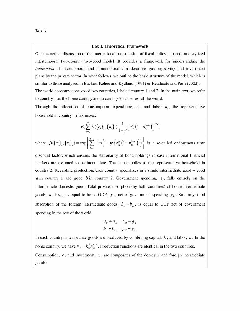
Boxes

Box 1. Theoretical Framework

Our theoretical discussion of the international transmission of fiscal policy is based on a stylized

intertemporal two-country two-good model. It provides a framework for understanding the

interaction of intertemporal and intratemporal considerations guiding saving and investment

plans by the private sector. In what follows, we outline the basic structure of the model, which is

similar to those analyzed in Backus, Kehoe and Kydland (1994) or Heathcote and Perri (2002).

The world economy consists of two countries, labeled country 1 and 2. In the main text, we refer

to country 1 as the home country and to country 2 as the rest of the world.

Through the allocation of consumption expenditure, 1c , and labor 1n , the representative

household in country 1 maximizes:

{ } { } ( ) 11

0 1 1 1, 1,0

1( , ) 1

1 t tt tt

E c n c nγµ µβ

γ

∞ −−

=

� �−� �−� ,

where { } { } ( ){ }( )11

1 1 1 10

( , ) exp ln 1 1t

t tc n c nµ µ

τ ττ

β ψ−

−

=

� �= − + −� �� �� is a so-called endogenous time

discount factor, which ensures the stationarity of bond holdings in case international financial

markets are assumed to be incomplete. The same applies to the representative household in

country 2. Regarding production, each country specializes in a single intermediate good – good

a in country 1 and good b in country 2. Government spending, g , falls entirely on the

intermediate domestic good. Total private absorption (by both countries) of home intermediate

goods, 1 2t ta a+ , is equal to home GDP, 1ty , net of government spending 1tg . Similarly, total

absorption of the foreign intermediate goods, 1 2t tb b+ , is equal to GDP net of government

spending in the rest of the world:

1 2 1 1

1 2 2 2

t t t t

t t t t

a a y g

b b y g

+ = −+ = −

In each country, intermediate goods are produced by combining capital, k , and labor, n . In the

home country, we have 11 1 2t t ty k nθ θ−= . Production functions are identical in the two countries.

Consumption, c , and investment, x , are composites of the domestic and foreign intermediate

goods:

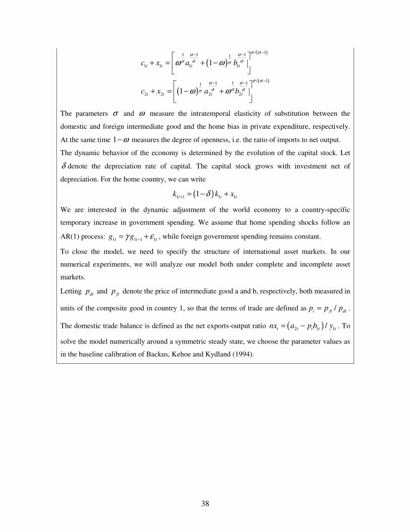
38

( )( )

( )( )

/ 11 1 11

1 1 1 1

/ 11 1 11

2 2 2 2

1

1

t t t t

t t t t

c x a b

c x a b

σ σσ σσ σ σσ

σ σσ σσ σ σσ

ω ω

ω ω

−− −

−− −

� �+ = + −� �

� �

� �+ = − +� �

� �

The parameters σ and ω measure the intratemporal elasticity of substitution between the

domestic and foreign intermediate good and the home bias in private expenditure, respectively.

At the same time 1 ω− measures the degree of openness, i.e. the ratio of imports to net output.

The dynamic behavior of the economy is determined by the evolution of the capital stock. Let

δ denote the depreciation rate of capital. The capital stock grows with investment net of

depreciation. For the home country, we can write

( )1 1 1 11t t tk k xδ+ = − +

We are interested in the dynamic adjustment of the world economy to a country-specific

temporary increase in government spending. We assume that home spending shocks follow an

AR(1) process: 1 1 1 1t t tg gγ ε−= + , while foreign government spending remains constant.

To close the model, we need to specify the structure of international asset markets. In our

numerical experiments, we will analyze our model both under complete and incomplete asset

markets.

Letting dtp and ftp denote the price of intermediate good a and b, respectively, both measured in

units of the composite good in country 1, so that the terms of trade are defined as /t ft dtp p p= .

The domestic trade balance is defined as the net exports-output ratio ( )2 1 1/t t t t tnx a p b y= − . To

solve the model numerically around a symmetric steady state, we choose the parameter values as

in the baseline calibration of Backus, Kehoe and Kydland (1994).

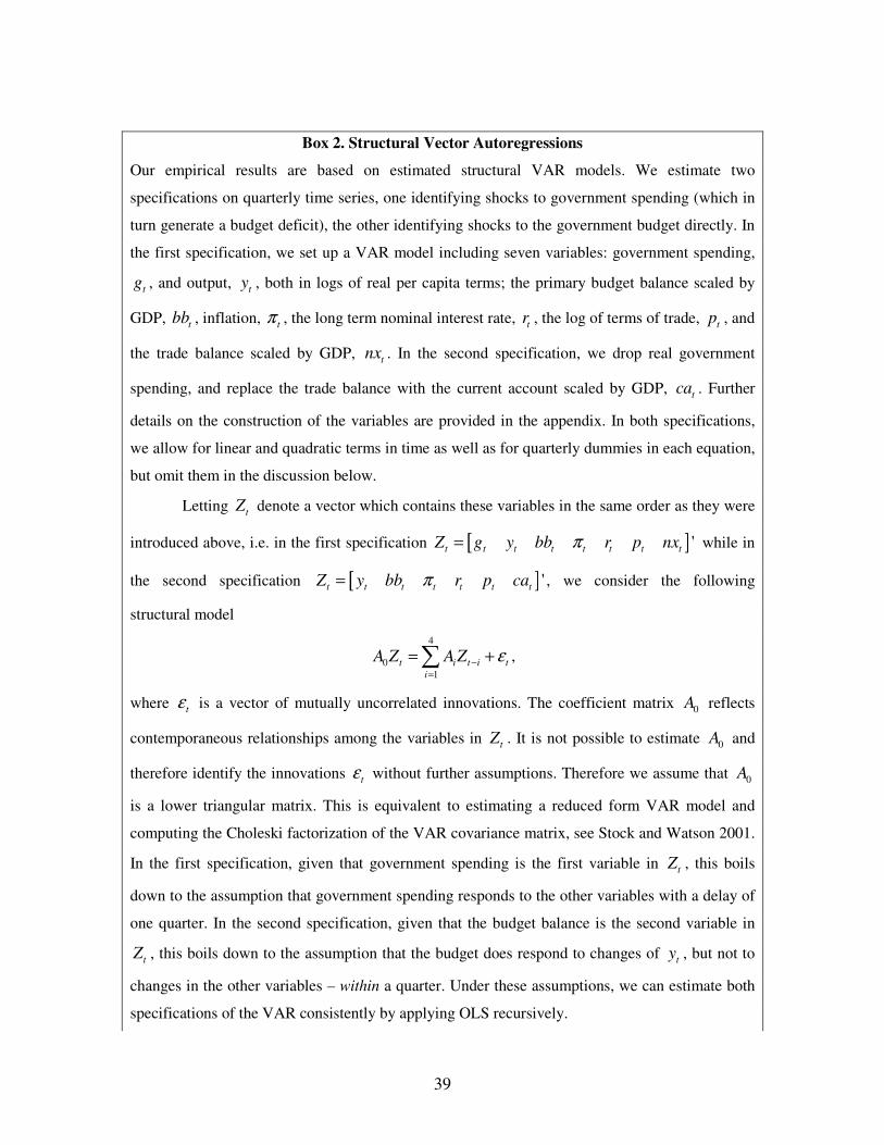
39

Box 2. Structural Vector Autoregressions

Our empirical results are based on estimated structural VAR models. We estimate two

specifications on quarterly time series, one identifying shocks to government spending (which in

turn generate a budget deficit), the other identifying shocks to the government budget directly. In

the first specification, we set up a VAR model including seven variables: government spending,

tg , and output, ty , both in logs of real per capita terms; the primary budget balance scaled by

GDP, tbb , inflation, tπ , the long term nominal interest rate, tr , the log of terms of trade, tp , and

the trade balance scaled by GDP, tnx . In the second specification, we drop real government

spending, and replace the trade balance with the current account scaled by GDP, tca . Further

details on the construction of the variables are provided in the appendix. In both specifications,

we allow for linear and quadratic terms in time as well as for quarterly dummies in each equation,

but omit them in the discussion below.

Letting tZ denote a vector which contains these variables in the same order as they were

introduced above, i.e. in the first specification [ ]'t t t t t t t tZ g y bb r p nxπ= while in

the second specification [ ]'t t t t t t tZ y bb r p caπ= , we consider the following

structural model

4

01

t i t i ti

A Z A Z ε−=

= +� ,

where tε is a vector of mutually uncorrelated innovations. The coefficient matrix 0A reflects

contemporaneous relationships among the variables in tZ . It is not possible to estimate 0A and

therefore identify the innovations tε without further assumptions. Therefore we assume that 0A

is a lower triangular matrix. This is equivalent to estimating a reduced form VAR model and

computing the Choleski factorization of the VAR covariance matrix, see Stock and Watson 2001.

In the first specification, given that government spending is the first variable in tZ , this boils

down to the assumption that government spending responds to the other variables with a delay of

one quarter. In the second specification, given that the budget balance is the second variable in

tZ , this boils down to the assumption that the budget does respond to changes of ty , but not to

changes in the other variables – within a quarter. Under these assumptions, we can estimate both

specifications of the VAR consistently by applying OLS recursively.

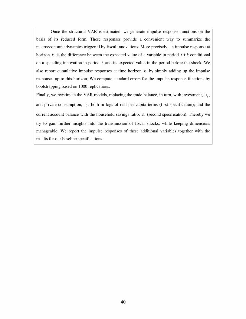
40

Once the structural VAR is estimated, we generate impulse response functions on the

basis of its reduced form. These responses provide a convenient way to summarize the

macroeconomic dynamics triggered by fiscal innovations. More precisely, an impulse response at

horizon k is the difference between the expected value of a variable in period t k+ conditional

on a spending innovation in period t and its expected value in the period before the shock. We

also report cumulative impulse responses at time horizon k by simply adding up the impulse

responses up to this horizon. We compute standard errors for the impulse response functions by

bootstrapping based on 1000 replications.

Finally, we reestimate the VAR models, replacing the trade balance, in turn, with investment, tx ,

and private consumption, tc , both in logs of real per capita terms (first specification); and the

current account balance with the household savings ratio, ts (second specification). Thereby we

try to gain further insights into the transmission of fiscal shocks, while keeping dimensions

manageable. We report the impulse responses of these additional variables together with the

results for our baseline specifications.

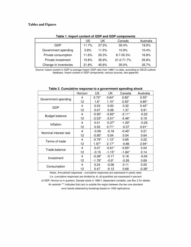
Tables and Figures

Table 1. Import content of GDP and GDP components US UK Canada Australia

GDP 11.7% 27.3% 30.4% 19.0%

Government spending 5.8% 11.5% 10.9% 10.4%

Private consumption 11.6% 20.3% 8.7-20.3% 16.8%

Private investment 15.8% 35.9% 21.0-71.7% 25.8%

Change in inventories 21.8% 45.6% 35.0% 35.7% Source: import content in GDP is average import–GDP ratio from 1980:1 to date, according to OECD outlook

database. Import content in GDP components: various sources, see appendix

Table 2. Cumulative response to a government spending shock Horizon US UK Canada Australia

4 0.72* 0.64* 0.82* 0.55* Government spending 12 1.6* 1.15* 2.55* 0.85* 4 0.53 0.00 0.32 0.42* GDP 12 0.07 0.08 1.37 0.91 4 -0.95* -0.83* -2.11* -0.22 Budget balance 12 -2.53* -3.51* -5.46* 0.19 4 0.01 -0.37* -1.29* -0.29 Inflation 12 0.50 0.71* -0.37 0.91* 4 -0.09 -0.18 -0.45* 0.21 Nominal interest rate 12 -0.95* 0.04 0.04 0.64 4 -0.79* 1.13* 0.85 0.22 Terms of trade 12 1.97* 2.17* -0.86 2.94* 4 0.07 -0.61* -0.65* 0.04 Trade balance 12 -0.15 -1.15* -1.84* 0.14 4 -0.28* -0.17 0.18 -0.04 Investment 12 -1.78* -0.9* -0.26 0.69 4 0.24 -0.06 0.11 0.00 Consumption 12 0.47 -0.12 0.68 -0.38*

Notes. Annualized responses - cumulative responses are expressed in yearly rates

(i.e. cumulative responses are divided by 4); all quantities are expressed in percent

of GDP; Horizon is in quarters. Sample starts in 1980:1 (dependent variable), see Box 2 for details.

An asterisk "*" indicates that zero is outside the region between the two one-standard

error bands obtained by bootstrap based on 1000 replications.

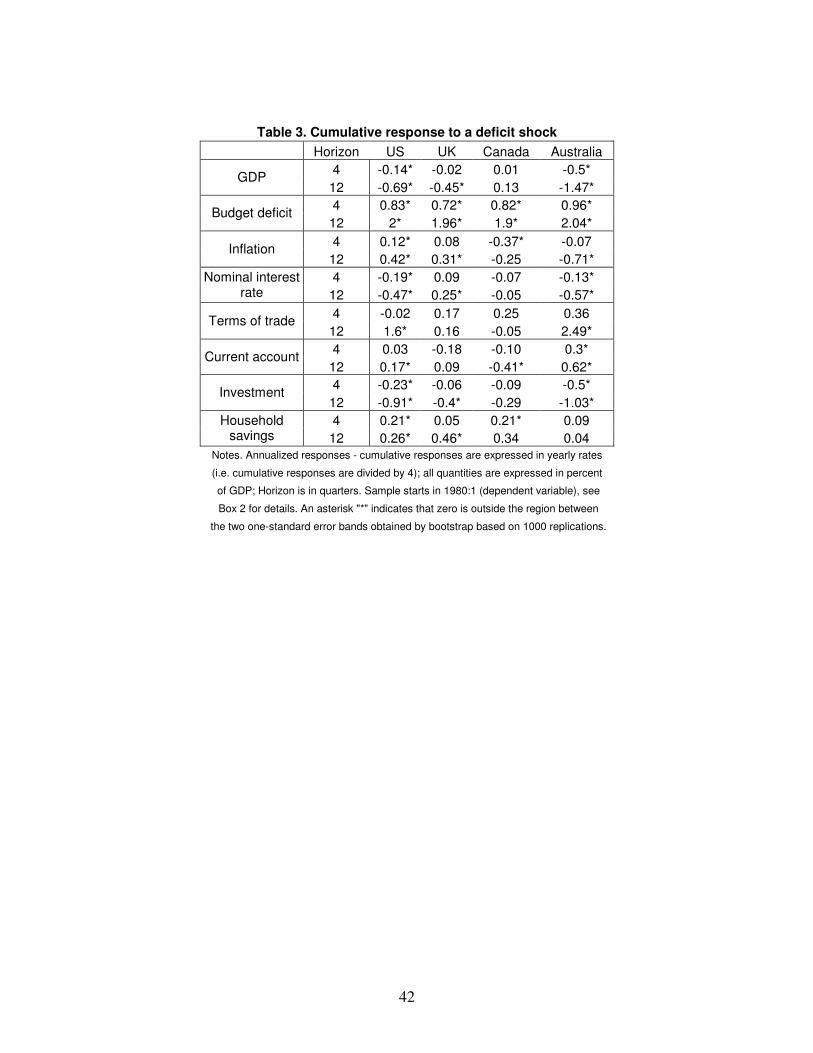
42

Table 3. Cumulative response to a deficit shock Horizon US UK Canada Australia

4 -0.14* -0.02 0.01 -0.5* GDP 12 -0.69* -0.45* 0.13 -1.47* 4 0.83* 0.72* 0.82* 0.96* Budget deficit 12 2* 1.96* 1.9* 2.04* 4 0.12* 0.08 -0.37* -0.07 Inflation 12 0.42* 0.31* -0.25 -0.71* 4 -0.19* 0.09 -0.07 -0.13* Nominal interest

rate 12 -0.47* 0.25* -0.05 -0.57* 4 -0.02 0.17 0.25 0.36 Terms of trade 12 1.6* 0.16 -0.05 2.49* 4 0.03 -0.18 -0.10 0.3* Current account 12 0.17* 0.09 -0.41* 0.62* 4 -0.23* -0.06 -0.09 -0.5* Investment 12 -0.91* -0.4* -0.29 -1.03* 4 0.21* 0.05 0.21* 0.09 Household

savings 12 0.26* 0.46* 0.34 0.04 Notes. Annualized responses - cumulative responses are expressed in yearly rates

(i.e. cumulative responses are divided by 4); all quantities are expressed in percent

of GDP; Horizon is in quarters. Sample starts in 1980:1 (dependent variable), see

Box 2 for details. An asterisk "*" indicates that zero is outside the region between

the two one-standard error bands obtained by bootstrap based on 1000 replications.

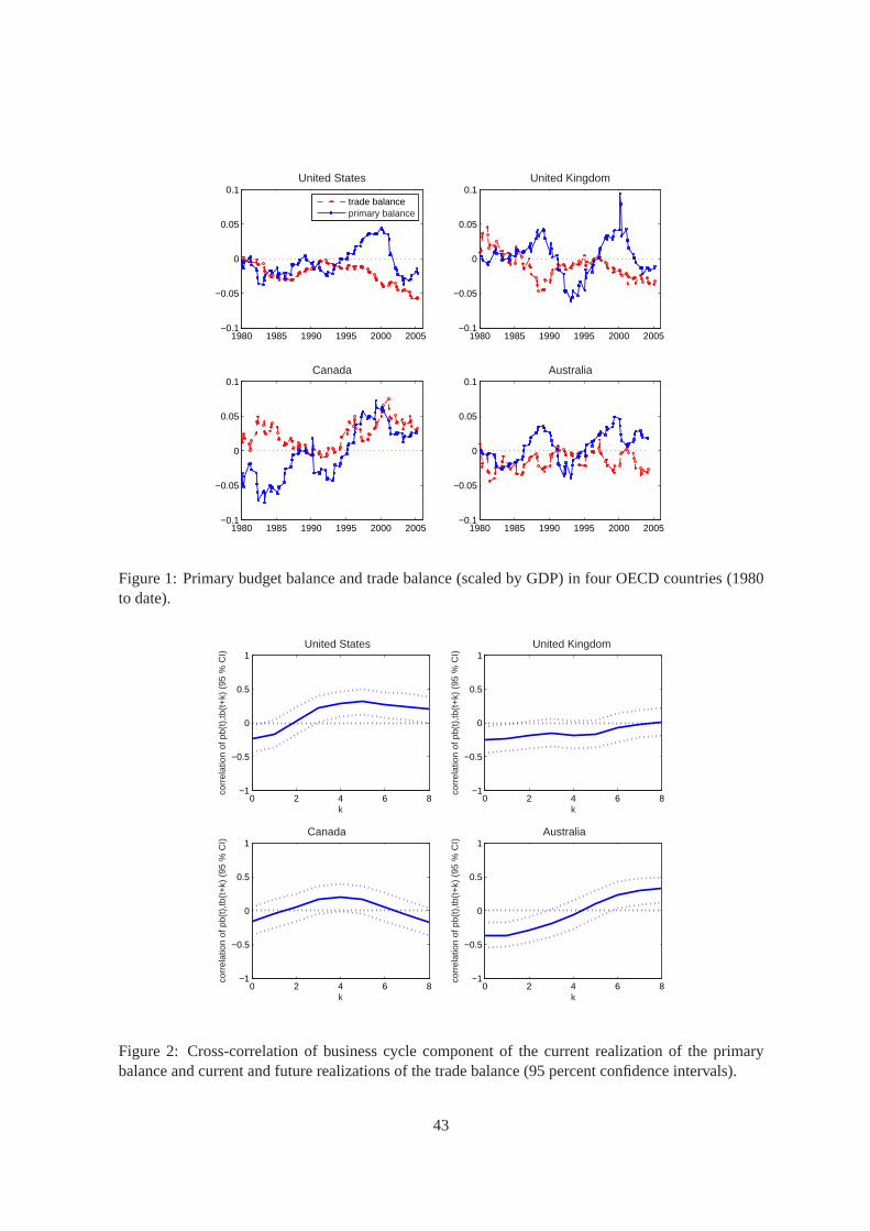
1980 1985 1990 1995 2000 2005−0.1

−0.05

0

0.05

0.1United States

trade balanceprimary balance

1980 1985 1990 1995 2000 2005−0.1

−0.05

0

0.05

0.1United Kingdom

1980 1985 1990 1995 2000 2005−0.1

−0.05

0

0.05

0.1Canada

1980 1985 1990 1995 2000 2005−0.1

−0.05

0

0.05

0.1Australia

Figure 1: Primary budget balance and trade balance (scaled by GDP) in four OECD countries (1980to date).

0 2 4 6 8−1

−0.5

0

0.5

1United States

corr

elat

ion

of p

b(t)

,tb(t

+k)

(95

% C

I)

k0 2 4 6 8

−1

−0.5

0

0.5

1United Kingdom

corr

elat

ion

of p

b(t)

,tb(t

+k)

(95

% C

I)

k

0 2 4 6 8−1

−0.5

0

0.5

1Canada

corr

elat

ion

of p

b(t)

,tb(t

+k)

(95

% C

I)

k0 2 4 6 8

−1

−0.5

0

0.5

1Australia

corr

elat

ion

of p

b(t)

,tb(t

+k)

(95

% C

I)

k

Figure 2: Cross-correlation of business cycle component of the current realization of the primarybalance and current and future realizations of the trade balance (95 percent confidence intervals).

43

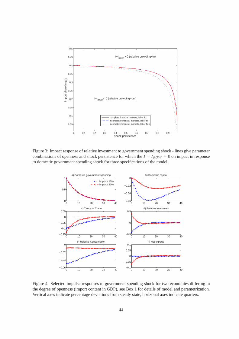
shock persistence

impo

rt s

hare

in g

dp

I−IROW

> 0 (relative crowding−in)

I−IROW

< 0 (relative crowding−out)

0 0.1 0.2 0.3 0.4 0.5 0.6 0.7 0.8 0.9

0.05

0.1

0.15

0.2

0.25

0.3

0.35

0.4

0.45

0.5

complete financial markets, labor fixincomplete financial markets, labor fixincomplete financial markets, labor flex

Figure 3: Impact response of relative investment to government spending shock - lines give parametercombinations of openness and shock persistence for which theI − IROW = 0 on impact in responseto domestic government spending shock for three specifications of the model.

0 10 20 30 400

0.5

1a) Domestic government spending

Imports 10%Imports 30%

0 10 20 30 40−0.06

−0.04

−0.02

0b) Domestic capital

0 10 20 30 40−0.15

−0.1

−0.05

0

0.05c) Terms of Trade

0 10 20 30 40−0.5

0

0.5d) Relative Investment

0 10 20 30 40−0.06

−0.04

−0.02

0e) Relative Consumption

0 10 20 30 40−0.1

−0.05

0

0.05

0.1f) Net exports

Figure 4: Selected impulse responses to government spending shock for two economies differing inthe degree of openness (import content in GDP), see Box 1 for details of model and parametrization.Vertical axes indicate percentage deviations from steady state, horizonal axes indicate quarters.

44

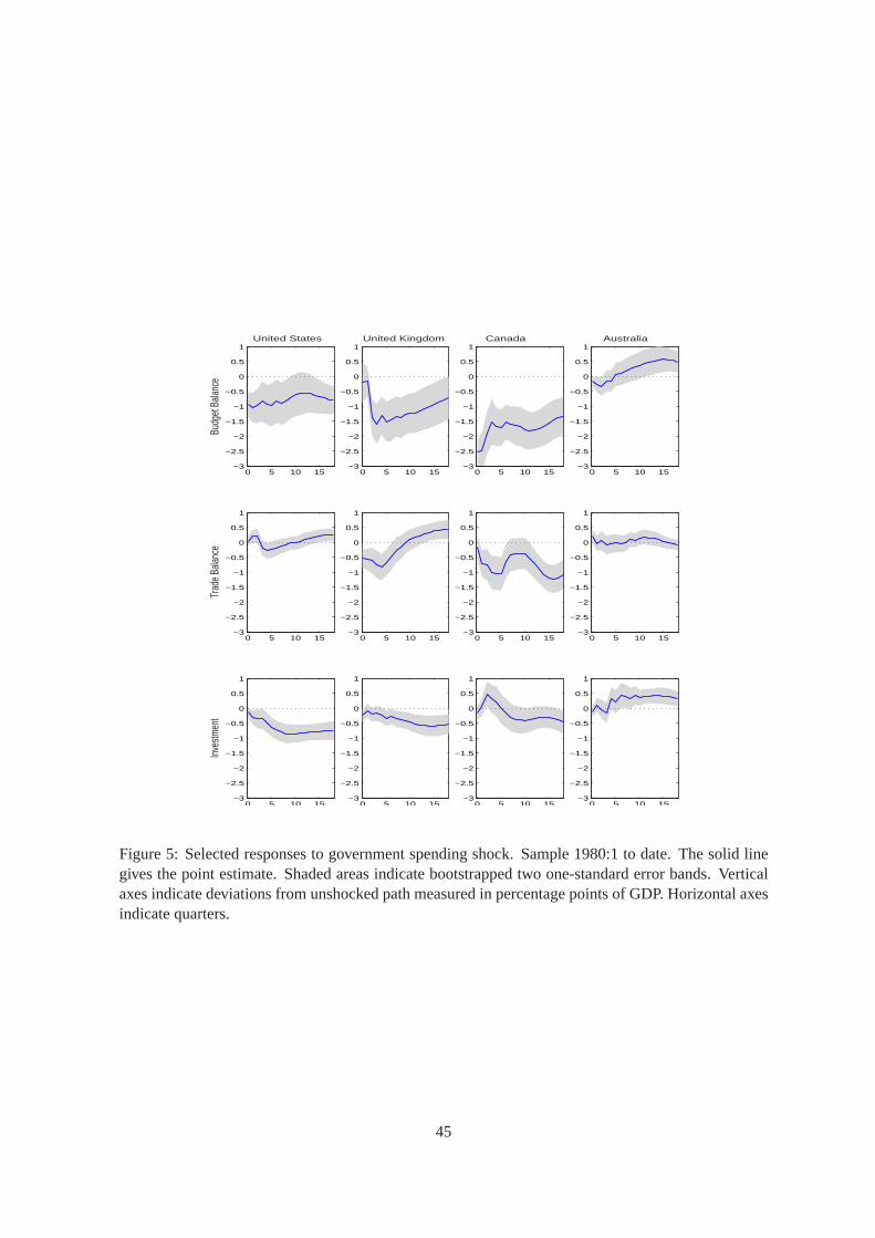
0 5 10 15−3

−2.5

−2

−1.5

−1

−0.5

0

0.5

1United States

Budg

et B

alanc

e

0 5 10 15−3

−2.5

−2

−1.5

−1

−0.5

0

0.5

1United Kingdom

0 5 10 15−3

−2.5

−2

−1.5

−1

−0.5

0

0.5

1Canada

0 5 10 15−3

−2.5

−2

−1.5

−1

−0.5

0

0.5

1Australia

0 5 10 15−3

−2.5

−2

−1.5

−1

−0.5

0

0.5

1

Trad

e Ba

lance

0 5 10 15−3

−2.5

−2

−1.5

−1

−0.5

0

0.5

1

0 5 10 15−3

−2.5

−2

−1.5

−1

−0.5

0

0.5

1

0 5 10 15−3

−2.5

−2

−1.5

−1

−0.5

0

0.5

1

0 5 10 15−3

−2.5

−2

−1.5

−1

−0.5

0

0.5

1

Inve

stmen

t

0 5 10 15−3

−2.5

−2

−1.5

−1

−0.5

0

0.5

1

0 5 10 15−3

−2.5

−2

−1.5

−1

−0.5

0

0.5

1

0 5 10 15−3

−2.5

−2

−1.5

−1

−0.5

0

0.5

1

Figure 5: Selected responses to government spending shock. Sample 1980:1 to date. The solid linegives the point estimate. Shaded areas indicate bootstrapped two one-standard error bands. Verticalaxes indicate deviations from unshocked path measured in percentage points of GDP. Horizontal axesindicate quarters.

45

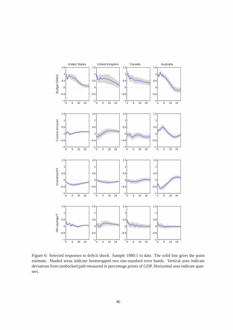
0 5 10 15−1

−0.5

0

0.5

1

1.5United States

Bud

get D

efic

it

0 5 10 15−1

−0.5

0

0.5

1

1.5United Kingdom

0 5 10 15−1

−0.5

0

0.5

1

1.5Canada

0 5 10 15−1

−0.5

0

0.5

1

1.5Australia

0 5 10 15−1

−0.5

0

0.5

1

1.5

Cur

rent

Acc

ount

0 5 10 15−1

−0.5

0

0.5

1

1.5

0 5 10 15−1

−0.5

0

0.5

1

1.5

0 5 10 15−1

−0.5

0

0.5

1

1.5

0 5 10 15−1

−0.5

0

0.5

1

1.5

Inve

stm

ent/Y

0 5 10 15−1

−0.5

0

0.5

1

1.5

0 5 10 15−1

−0.5

0

0.5

1

1.5

0 5 10 15−1

−0.5

0

0.5

1

1.5

0 5 10 15−1

−0.5

0

0.5

1

1.5

HH

sav

ings

/Y

0 5 10 15−1

−0.5

0

0.5

1

1.5

0 5 10 15−1

−0.5

0

0.5

1

1.5

0 5 10 15−1

−0.5

0

0.5

1

1.5

Figure 6: Selected responses to deficit shock. Sample 1980:1 to date. The solid line gives the pointestimate. Shaded areas indicate bootstrapped two one-standard error bands. Vertical axes indicatedeviations from unshocked path measured in percentage points of GDP. Horizontal axes indicate quar-ters.

46