St. Cloud State UniversitytheRepository at St. Cloud State

Economics Faculty Working Papers Department of Economics

2011

Twin Deficits or Distant Cousins? Evidence fromIndiaArtatrana RathaSt. Cloud State University, aratha@stcloudstate.edu

Follow this and additional works at: https://repository.stcloudstate.edu/econ_wps

Part of the Economics Commons

This Working Paper is brought to you for free and open access by the Department of Economics at theRepository at St. Cloud State. It has beenaccepted for inclusion in Economics Faculty Working Papers by an authorized administrator of theRepository at St. Cloud State. For more information,please contact rswexelbaum@stcloudstate.edu.

Recommended CitationRatha, Artatrana, "Twin Deficits or Distant Cousins? Evidence from India" (2011). Economics Faculty Working Papers. 5.https://repository.stcloudstate.edu/econ_wps/5

1

Twin Deficits or Distant Cousins? Evidence from India*

Artatrana Ratha Associate Professor

Department of Economics St. Cloud State University

St. Cloud, MN 56301 aratha@stcloudstate.edu

Abstract: The twin-deficits theory has intrigued economists and policy-makers alike for

the past few decades. In a Keynesian economy, budget deficit increases the absorption of the

economy, causes import expansions, and thereby, worsens the trade deficit. It also causes

domestic interest rates to rise, domestic currency to appreciate, and thereby, contributes to trade

deficits. However, according to the Ricardian Equivalence Hypothesis (REH), rising budget

deficits implies higher future tax-liabilities so people would save more and consume less. As a

result, an inter-temporal shift between taxes and budget deficits would have no impact on the real

interest, or the trade deficit. Thus, the issue of whether the twin-deficits phenomenon holds

becomes more of an empirical question, and the recent fiscal expansions to curb recession makes

it timely to revisit the phenomenon, especially for the developing countries confronting both the

deficits on a chronic basis. To this end, we make a case study of India, using the bounds-testing

approach to cointegration and error-correction modeling on monthly and quarterly data over

1998-2009. Our results suggest that the twin-deficits theory holds for India in the short-run

(validating the Keynesian channel) but not in the long run (validating the REH).

Key Word: Bounds-Testing, Budget Deficit, Fiscal Stimulus, India, Trade Deficit, Twin Deficits

JEL Classification: F 32, H 62

* The title of the paper was inspired by Enders and Lee (1990). The author thankfully acknowledges valuable comments from an anonymous referee. The usual disclaimer applies.

2

Twin Deficits or Distant Cousins? Evidence from India

I. Introduction

Fiscal stimulus is a buzz word today. In trying to catapult their flailing economies,

Governments world over have resorted to fiscal stimuli and embraced escalations in budget

deficits. Despite the slowdown in economy activity, current account deficits have not subsided

either, especially in India, where inflation has accelerated to 10.7% and the Government is under

pressure to rein in the budget deficit from a 16-year high of 6.8% to a more reasonable level.1

Moreover, will a reduction in budget deficit help improve her trade deficit which has been

trending up since the mid-90s? While a growing trade deficit may not necessarily be a cause of

concern for a growing economy, trade deficit coupled with increasing budget deficit and the

resultant inflation could lower the country’s sovereign ratings and trigger a capital flight,

reminiscent of the Asian crisis, or the recent chaos in the euro-area. Deficit reductions, while

difficult, need to be the guiding principle in the forthcoming budget.

Interestingly budget deficit and trade deficit, commonly known as the twin-deficits, tend

to go hand in hand, and, if they indeed do, establishing their causality will go a long way in

formulating public policy. Accordingly, a vast body of literature has come up trying to establish

the nexus between the two deficits. In terms of theory, the literature has evolved along two broad

strands, viz. the conventional (or Keynesian) approach and the neoclassical (or Ricardian)

approach: the conventional approach establishes a link between budget deficit and trade deficit;

the neoclassical approach finds no such relationships. Given this theoretical ambiguity and its

policy-implications, it is no surprise that the empirical literature examining the twin-deficits

phenomenon is quite rich.

3

For example, the Keynesian absorption theory asserts that budget deficits increase

domestic absorption which leads to import expansion and worsens the trade deficit. Also budget

deficits imply greater spending on domestic as well as foreign goods, the former pushing the

exports down and the latter pulling the imports up, especially in an economy with supply

bottlenecks. In a Mundell-Fleming model, budget deficits cause interest rates to rise (Cebula,

1988, 2003; Cebula and Rhodd, 1993; Modeste, 2000), surge in capital inflows, and currency

appreciation (Feldstein, 1986; Rosensweig and Tallman, 1993). Currency appreciation implies

imports get cheaper and exports dearer so trade deficit deteriorates (Bahmani-Oskooee and

Ratha, 2004; Bundt and Solocha, 1988; Piersanti, 2000). However, according to the Ricardian

Equivalence Hypothesis (REH), foreseeing higher tax-liabilities (due to current fiscal

expansions), people would save more and consume less. As a result, an intertemporal shift

between taxes and budget deficits would have no impact on the real interest, or the trade deficit

(Barro, 1974; Enders and Lee, 1990; Evans, 1988). Thus, if REH holds for a country, the

explanation for a persistent trade deficit must be found somewhere else such as international

competitiveness, capital mobility, etc. (Ahmed and Ansari, 1994). However, if it does not, i.e.

the twin-deficits phenomenon holds, then taming one deficit (depending on causality) will also

tame the other! While the results are mixed, it appears that the twin-deficits hypothesis generally

holds for the developed countries: budget deficits tend to worsen to trade deficits. See for

example, Bernheim (1988), Rosensweig and Tallman (1993), and for a recent literature survey,

Saleh and Harvie (2005).

For developing countries, however, the literature is rather sparse and the results mixed

(Kouassi, et. al, 2004). Some recent studies supporting the Keynsean channel (i.e., budget

deficit causing trade deficit) include Somadi (2006) for Egypt, Kulkarni and Ericsson (2001) for

4

India, Saleh and Nair (2006) for Philippines, Saleh, et al (2005) for Sri Lanka, Akbostanci and

Tunc (2006) for Turkey, although the models, methodology, and the sample period, vary quite a

bit.2 This paper contributes to this literature by reexamining the twin-deficits theory for India,

especially during the post-reforms era. Interestingly, almost all of the India-specific studies that

we came across are based on data from the pre-liberalization era.3 Ghatak and Ghatak (1996), for

example, employed multi-cointegration analysis on data over 1950-1986 and found no evidence

in favor of the REH, i.e., it is possible that the India’s budget and trade deficits could be related.

Indeed, using data over the 1965-1993 time-periods, Anuruo and Ramchander (1997, 1998)

found that trade deficit Granger causes budget deficit in India. Kulkarni and Ericsson (2001), on

the other hand, employed data over comparable time-period (viz. 1969-1996) but found the

contrary, i.e., budget deficit Granger causes trade deficit in India. Another study we came across

was by Kouassi, et al (2004) who found no casual relationship between the two on Indian data

over the 1975-97 time-period and suggested including additional macro-variables in the model.

Accordingly, in this paper, we employ a model involving more macro-variables, viz. domestic

and foreign incomes, real effective exchange rate, besides the two deficits. Moreover, we

improve on the previous approaches on three fronts: (i) we define the variables in non-negative,

real, and unit-free terms such that biases stemming from using different units are reduced and

also the model can be estimated in log form;4 (ii) we employ the bounds-testing approach,

proposed by Pesaran, et al (2001) – a relatively recent cointegration technique requiring no pre-

unit testing and is also deemed appropriate for small samples; and (iii) our sample comprises of

recent high frequency data, viz. monthly as well as quarterly data over 1998-2009 – a period

reflecting an advanced stage of economic reforms in India. The rest of the paper is organized as

follows: Section II provides an outline of the model and methodology, Section III discusses the

5

empirical results, and Section IV concludes. Data, definitions, and sources are cited in an

appendix.

II. Outline of the Model and Methodology

The national income identity for an open economy is:

Total income = Total expenditure,

i.e., C+S+T = C+I+G+(X-M) … (1)

where C=consumption, S=savings, T=taxes, I=investment, G=government expenditure,

X=exports, and M=imports. Rearranging terms yields:

(M-X)=(I-S) + (G-T),

i.e., 𝑀𝑋

= �1 + 𝐼−𝑆−𝑇𝑋

� + 𝑇𝑋

. 𝐺𝑇 … (2)

Equations (2) holds by definition. While it establishes a direct link between the budget and

current account deficits, it does not necessarily imply that they are twins, unless S and I are

strongly correlated. However, it provides the basis for a reduced form model such as:

ln TBt = α + β ln BDt +εt …(3)

which, in line with previous literature, is further augmented to include domestic and foreign

incomes, real effective exchange rate (Y, YF, RER, respectively) 1:

ln TBt = a + b ln Yt+ c ln YFt + d ln RERt + f ln BDt +εt …(4)

where the variables TBt is trade deficit defined as the ratio of imports to exports such that an

increase implies a deterioration of the trade balance; Yt and YFt are domestic and foreign incomes

respectively; RERt is the real effective exchange rate such that an increase implies an

appreciation of domestic currency; BDt is budget deficit measured by the ratio of expenditures to

receipts ratio of the government so that an increase implies an escalation of budget deficit. All

1 See for example Rose and Yellen (1989), Bahmani-Oskooee (2007).

6

variables are real. In fact, defining the trade deficit and the budget deficit in ratio-form is helpful

on two grounds: (i) there is no need to find a suitable price-index to deflate the nominal

variables to arrive at their real counterparts as the ratio is already real, and (ii) since they are

necessarily non-negative, they allow running the model in log form such that the coefficients are

actually the elasticities of trade deficit with respect to the corresponding variables (Rose and

Yellen, 1989).

The coefficients of the model are theoretically ambiguous, however. While presence of

income effects would imply positive coefficients for the income variables (i.e. Yt and YFt), it is

possible that the increase in the latter stems mostly from expansion of import competing

industries in which case they can take on negative coefficients. Likewise, unless the sum of

exports and imports demand elasticities add up to more than one, currency depreciation may or

may not boost the trade balance so d the coefficient of RERt can be positive as well as negative. 5

The same is true of f, the coefficient of budget deficit: if the Keynesian channel is dominant, it

will be positive; otherwise it would be negative and/or insignificant. Thus, the signs of the

coefficients are best determined empirically. Given the coexistence of high unemployment and

wage-price rigidities and the consequent adjustment lags, however, it appears that the Keynesian

model better characterizes the Indian economy.

The sample is comprised of monthly data over the past 11 years (viz. 1998:M1-2009:M3;

1998:Q1-2009:Q1), partly dictated by availability of data but deemed appropriate as: (i) the

period also reflects an advanced stage of the economic reforms that India launched in 1991, and

also (ii) the deficits seem to be escalating during this period. In the absence of monthly GDP

data for India, industrial production index is used as proxy. For an investigation of the twin-

deficits theory, cointegration and error correction modeling seems quite appropriate as the

7

technique helps decipher both the long run as well as the short-run dynamics. To avoid spurious

relations problem, it is necessary to pre-test the stationarity of the variables although tests tend to

lack robustness. Since the bounds-testing approach,6 proposed by Pesaran, et al (2001), requires

no pre unit-root testing and is also deemed appropriate for small sample sizes (Narayan, 2005) ,

we employ the technique to estimate equation (4). The error-correction mechanism for the long-

run equation (4) is specified as:

vtBDtRERtYFtY t

TBtri BD itbiq

i RERf i it

pi YFdi it

ni Yci it

mi TB itbiaTBt

+−+−+−+−+−+∑ = ∆ −+∑ = ∆ −+

∑ = ∆ −+∑ = ∆ −+∑ = ∆ −+=∆

15ln 14ln 13ln 12

ln 111 ln1 ln1 ln1 ln1 lnln

δδδδ

δ … (5)

where a linear combination of the lagged-level variables approximates the error-correction term.

The estimation procedure consists of three-steps:

(i) An F-Test where the null of no cointegration (i.e., 054321 ===== δδδδδ ) is

tested against its alternative (i.e., 054321 ≠≠≠≠≠ δδδδδ ). Pesaran, Shin, and Smith

(2001) provide a method of estimating the new critical values comprising of a lower

bound and an upper bound for large samples: If the calculated F-statistic falls above the

upper bound, the null hypothesis is rejected; if it falls below the lower bound the null

hypothesis cannot be rejected; if it falls in-between the results are inconclusive. Finally, a

negative and significant error-correction term would indicate cointegration among the

underlying variables. See for example, Kremers, et. al (1992).

(ii) A Choice of Optimal Lag-Structure is necessary because the F-test results are

sensitive to the lag-structure of the error-correction model. The Schwartz-Bayesian

Criterion (SBC) as well as the Akaike Information Criterion (AIC) are used to determine

the optimal lag structure.

8

(iii) The Long-run Model is estimated by normalizing the coefficients of the lagged

dependent variables in (5).

Finally, stability of the estimated coefficients is examined using the CUSUM and

CUSUMSQ test proposed by Brown, Durbin and Evans (1975).

III. Empirical Results

A glance at Figure 1(a) suggests that India’s budget deficit and trade deficit, both

expressed as a % of her GDP, have opposing trends, indicating no long run comovement

between the two. More precisely, budget deficits have been trending down since the early 90s

and trade deficits trending up since the mid-90s. However, both have their own short run spikes,

and are particularly surging up the past couple of years. Figure 1(b) presents the detrended values

of the deficits. Interestingly, it appears that the detrended values comoved during the 1980s but

have been countering each other since the early 1990s. Overall, they exhibit a meager correlation

of 0.13. However, this is only a preliminary observation calling for a more robust investigation

of the twin-deficits phenomenon. Accordingly, we proceed to estimate equation (2) by imposing

a maximum of 18 lags in case of monthly data and 4 lags in case of quarterly data (the maximum

that the data permitted) but the optimal lag-structure(s) are determined using the SBC as well as

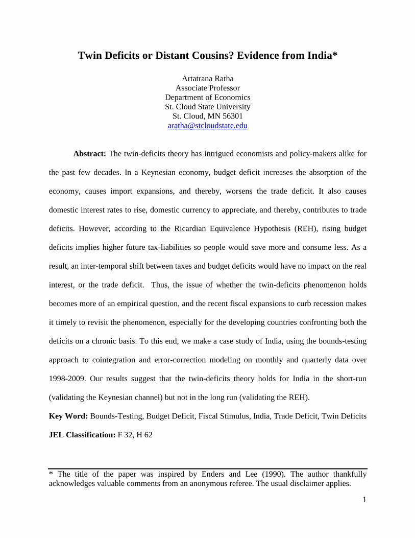
the AIC. The F-statistics corresponding to the optimum lag-structures are reported in Table 1,

panels A and B.

[Figure 1(a) and 1(b) go about here]

[Table 1 goes about here]

Given the lower and upper bounds of 2.645 and 4.805 (at 5% levels), respectively, the null

hypothesis of non-cointegration may be rejected for the SBC model but cannot be rejected for

the AIC model. However, according to Kremers, et. al (1992), if the lagged-error correction term

9

carries a significant, negative coefficient - as is the case here in Table 2 under both SBC and

AIC - there exists a long run relation among the variables. In fact the size of the coefficients

indicates relatively fast convergence to the long-run equilibrium in each case. Table 2 also

contains the coefficients of ∆ ln BDt-i, the variable of interest.7 In case of monthly data (Panel

A), it appears that budget deficits have no short run impact on trade deficit in the SBC model.

However, the AIC model points to the contrary: budget deficits contribute to the trade deficits in

the short-run! In case of quarterly data (Panel B), ∆ ln BDt is significant at the 10% level under

both SBC and AIC.8 These findings may suggest prevalence of the Keynesian channel in the

short-run.

[Table 2 goes about here]

Table 3 summarizes the long run relations. As may be noted, except for domestic income,

all of the variables are insignificant under both SBC and AIC, regardless of the frequency of

data. Of particular interest is the budget deficit carrying an insignificant coefficient in both cases,

providing evidence in favor of the REH in the long run. These findings are consistent with those

of Kouassi, et al (2004) for India.

[Table 2 goes about here]

Thus, it appears that the Keynesian channels explain the Indian data in the short-run but

fall through in the long run. This finding is consistent with those of Bachman (1992) for US

(1974-1988) and Kearney and Monadjemi (1990) for Australia, UK, Canada, France, Germany,

Ireland, Italy and the US (1972-1987).

How stable are our estimates? For this, CUSUM and CUSUMSQ statistics are plotted

against their break points in Figure 2 for the SBC model, and Figure 3 for the AIC model.

10

Interestingly, the coefficients estimates are stable in most cases, except for some instability under

CUSUMSQ in case of monthly data (Panel A in Figures 2 and 3).

[Figures 2 and 3 go about here]

IV. Summary and Concluding Remarks

The twin-deficits theory has intrigued economists and policy-makers alike for the past

few decades. In a Keynesian economy, budget deficit increases the absorption of the economy,

causes import expansions, and thereby, worsens the trade deficit. It also causes domestic interest

rates to rise, domestic currency to appreciate, and thereby, contributes to trade deficits. Using

monthly and quarterly data over 1998-2009 and the bounds testing approach to cointegration, we

find evidence that the twin-deficits theory holds for India in the short-run. Thus, by exercising

fiscal restraint, the Government of India should be able to rein in on the country’s trade deficit in

the short run. In the long run, fiscal discipline as such a policy tool loses its significance. The

latter finding is supportive of the Ricardian Equivalence Hypothesis (REH) that negates any

relationship between two deficits. Therefore, apart from the foregoing policy-implication, this

finding may help reconcile the two dominant views in the literature: the Keynesian views prevail

in the short run, and the neo-classical in the long run.

However, how long is the long run? Also, going by Keynes’ famous quote ‘in the long

run we all are dead!’, it only seems prudent to reduce the budget deficit, although it is easier said

than done. More so for a for a developing country like India whose growth trajectory calls for

ever increasing spending on power generation, infrastructure building (see, for example, Mallick,

2001) , not to mention the anti-poverty measures including provision of basic necessities to a

booming population. Thus, of necessity, fiscal discipline has to come mostly from the revenue

side where there is room for growth: tax-reforms targeted at broadening the tax-base (by taxing

11

hitherto untaxed or under-taxed sectors including the parallel economy), cutting tax-loopholes,

and minimizing tax-evasion. It appears that mitigating corruption will go a long way in boosting

the tax revenue as well as achieving both internal and external balance.

12

References

Ahmed, S. M. and Ansari, M. I., 1994. A Tale of Two Deficits: An Empirical Investigation for

Canada. The International Trade Journal, VIII, No. 4, Winter, 483-503.

Akbostanci, E. and Tunc, G. I, 2002. Turkish Twin Deficits: An Error Correction Model of

Trade Balance, ERC Working Papers in Economics, 01/06.

Anuruo, E. and Ramchander, S. 1997. Current Account and Fiscal Deficts: Evidence from India,

Indian Economic Journal, 45(3), 66-80.

Anuruo, E. and Ramchander, S. 1998. Current Account and Fiscal Deficts: Evidence from Five

Developing Economies of Asia, Journal of Asian Economics, 9(3), 487-501.

Akbostanci, E. and Tunc, G. I, 2002. Turkish Twin Deficits: An Error Correction Model of

Trade Balance, ERC Working Papers in Economics, 01/06.

Bahmani-Oskooee, M. 2007. Do budget deficits contribute to trade deficits in Spain?,

Informacion Comercial Espanola. Revista de Economia, 835, March-April, 7-23.

Bahmani-Oskooee, M., and Ratha, A. 2004. The J-Curve: A Literature Review, Applied

Economics, 36, 1377-1398.

Barro, R. J. , 1974. Are government bonds net wealth?, Journal of Political Economy, 82, 1095–1117.

Brown, R.L., Durbin, J., Evans, J.M., 1975. Techniques for Testing the Constancy of Regression

Relationships over Time, Journal of the Royal Statistical Society, Series B 37, 149–192.

Bachman, D., 1992. Why is the US Current Account Deficit so Large? Southern Economic

Journal, 59, 232-240.

Bernheim, D. B. 1988. Budget Deficits and the Balance of Trade, Tax Policy and the Economy,

Cambridge: MIT Press, 1-31.

Bundt, T. and Soloch, A., 1988. Debt, Deficits, and Dollar, Journal of Policy Modelling, 10(4),

581-600.

Cebula, R. 1988. Federal Government Deficits and interests in the US: A Brief Note. Southern

Economic Journal, 55(1), 206-210

Cebula, R. 1988. and Rhodd, R. (1993). A Note on Budget Deficits, Debt Service Payments,

and Interest Rates, The Quarterly Review of Economics and Finance, 33, 439-445.

Cebula, R. 2003. Budget Deficits and Interest Rates in Germany, International Advances in

Economic Research, 9(1), 64-68.

13

Enders, W. and Lee, B. S., 1990. Current Account and Budget Deficits: Twins or Distant

Cousins? The Review of Economics and Statistics, 72, 373-381.

Evans, P., 1988. Are Consumers Ricardian? Evidence from United States. Journal of Political

Economy, 96, 983-1004.

Fedstein, M. 1986. The Budget Deficit and the Dollar, NBER Macroeconomics Annual, edited

by Stanley Fischer, Cambridge, MIT Press, 355-92.

Ghatak, A., and Ghatak, S., 1996. Budgetary deficits and Ricardian equivalence: The case of

India, 1950-1986, Journal of Public Economics, 60 (2): 267-282.

Kearney, C. and Monadjemi, M., 1990. Fiscal and Current Account Performance: International

Evidence on Twin Deficits, Journal of Macroeconomics, 12, 197-220.

Kouassi, E., Mougoué, M. and Kymn, K.O., 2004. Causality tests of the relationship between

the twin deficits, Empirical Economics, 29 (3): 503-525

Kremers, J. J. M., Ericsson, N. R., and Dolado, J. J. 1992. The Power of Cointegration Tests,

Oxford Bulletin of Economics and Statistics, 54, 325-348.

Kulkarni, K. G. and Erickson, E. L, 2001. Twin Deficit Revisited: Evidence from India,

Pakistan, and Mexico, The Journal of Applied Business Research, 17 (2), 97-103.

Mallick, S. K., 2001. Dynamics of Macroeconomic Adjustment with Growth: Some Simulation

Results, International Economic Journal, 15(1), Spring, 115-139.

Modeste, N. C., 2000. The Impact of Budget Deficits on Long-Term Interest Rate in Jamaica,

1964-1996: An Application of the Eroor Correction Methodology, International Review of

Economics and Business, 47(4), 667-678.

Narayan, P. K., 2005. The Saving and Investment Nexus for China: Evidence from Cointegration

Tests, Applied Economics, 37, 1979-90.

Pesaran, M. H, Shin, Y, and Smith, R. J. 2001. Bounds Testing Approaches to the Analysis of

Level Relationships, Journal of Applied Econometrics, 16, 289-326.

Piersanti, G., 2000. Current Account Dynamics and Expected Future Budget Deficits: Some

International Evidence, Journal of International Money and Finance, 19(2), 2555-2571.

Rose, A. K.. and Yellen, J. L. 1989, ‘Is there a J-Curve?’ Journal of Monetary Economics, 24,

July, 53-68.

Rosensweig, J. A. and Tallman, E. W. 1993. Fiscal Policy and Trade Adjustment: Are the

Deficits Really Twins?, Economic Inquiry, XXXI, October, 580-594.

14

Samadi, A. H. 2006. The Twin Deficits Phenomenon in some MENA Countries, Iranian

Economic Review, 10(16), Spring, 129-139.

Saleh, A. S., Nair, M., and Agalewatte, T., 2005. The Twin Deficits Problem in Sri Lanka: An

Econometric Analysis, South Asia Economic Journal, 2(6), 221-239.

Saleh, A. S. and Harvie, C., 2005. The Budget Deficit and Economic Performance: A Survey,

The Singapore Economic Review, 50(2), 211-243.

Saleh, A. S. and Nair, M., 2006. The Twin deficits Phenomena in Philippines: An Empirical

Investigation, International Journal of Economic Research, 3(2), 165-179.

15

Appendix I

Data, Definitions, and Sources

Monthly data over 1998:1-2009:9 and quarterly data over 1998Q1-2009Q1 are collected

from various sources:

TB= India’s trade balance, defined as imports over exports of goods and services; an increase in

TB implies a deterioration of her trade balance. Exports and imports data are collected from the

International Financial Statistics of the IMF.

Y = GDP index (volume). In the absence of monthly data on GDP, India’s industrial production

index was used as a proxy for her real GDP; Collected from the International Financial Statistics

of the IMF.

YF = Industrial production index of the advanced economies, used as a proxy for the real income

of the rest of the world; Collected from the International Financial Statistics of the IMF.

RER = Real effective exchange rate of the Indian National Rupee, collected from the Bank of

International Settlement website.

BD = India’s budget deficit, defined as total government expenditures over total receipts such

that an increase implies an increase in budget deficit. Expendires and receipts data are from the

CGA of India website (Controller General of Accounts, Department of Expenditure, Ministry of

Finance, Government of India). Quarterly data were based on monthly data from the above

source.

16

Table 1. Cointegration Test Results

Panel A: Monthly Data (January, 1998 – September, 2009)

Criterion Lag-Structure Calculated Value of the F-Statistic

Schwartz Bayesian Criterion (SBC) (1, 1, 3, 0, 0) 7.92*

Akaike Information Criterion (AIC) (18, 17, 15, 1, 16) 2.19

Notes: For the lag-structure (i, j, k, l, m) implies i lags for the first variable, j lags for the second, and so on; an * denotes significance at 5% levels; the corresponding critical value is 3.805.

Panel B: Quarterly Data (1998Q1-2009Q1)

Criterion Lag-Structure Calculated Value of the F-Statistic

Schwartz Bayesian Criterion (SBC) (4, 0, 3, 1, 1) 4.13*

Akaike Information Criterion (AIC) (4, 3, 3, 3, 1) 2.46

Notes: For the lag-structure (i, j, k, l, m) implies i lags for the first variable, j lags for the second, and so on; an * denotes significance at 5% levels; the corresponding critical value is 4.123.

17

Table 2. Short Run Model

Panel A: Monthly Data (January, 1998 – September, 2009)

Dependent Variable is ∆LTBt

Coefficient of Chosen by SBC Chosen by AIC

∆LBDt -0.05 (1.38)

0.04 (0.92)

∆LBDt-1 - 0.24 (1.63)

∆LBDt-2 - 0.24 (1.72)

∆LBDt-3 - 0.27* (1.92)

∆LBDt-4 - 0.28* (2.10)

∆LBDt-5 - 0.26* (2.03)

∆LBDt-6 - 0.29* (2.41)

∆LBDt-7 - 0.32* (2.79)

∆LBDt-8 - 0.31* (2.89)

∆LBDt-9 - 0.32* (3.19)

∆LBDt-10 - 0.28* (2.96)

∆LBDt-11 - 0.24* (2.79)

∆LBDt-12 - 0.17* (2.29)

∆LBDt-13 - 0.11** (1.75)

∆LBDt-14 - 0.04 (0.92)

∆LBDt-15 - 0.05 (1.43)

ECMt-1 -0.58* (6.61)

-0.72* (6.48)

Note: LBDt = ln BDt; Only coefficients of ∆LBDt-i , i=0, 1, 2, … and the lagged error-correction term, ECMt-1 are reported. Figures in parentheses are absolute values of the t-statistic; Asterisks * and ** denote significance at the 5% and 10% levels, respectively; a dash (-) indicates the corresponding variable does not appear in the model; ∆LBDt. = LBDt-LBDt-1, ∆LBDt-1=LBDt-1-LBDt-2, and so on.

18

Panel B: Quarterly Data (1998Q1-2009Q1)

Dependent Variable is ∆LTBt Coefficient of Chosen by SBC Chosen by AIC

∆LBDt 0.04** (1.87)

0.05** (1.89)

ECMt-1 -0.41* (2.88)

-0.34* (2.34)

Note: LBDt = ln BDt; ∆LBDt = LBDt-LBDt-1 . Only coefficients of ∆LBDt-i , i=0, 1, 2, … and the lagged error-correction term, ECMt-1 are reported. Figures in parentheses are absolute values of the t-statistic; Asterisks * and ** denote significance at the 5% and 10% levels, respectively.

Table 3. Long Run Model

Panel A: Monthly Data (January, 1998 – September, 2009)

Dependent Variable is ∆LTBt Coefficient of Chosen by SBC Chosen by AIC

Constant -4.31** (1.87)

0.41 (0.09)

LYt 0.45* (3.44)

0.76** (1.91)

LYFt 0.63

(0.96) -0.24 (0.14)

LRERt -0.07 (0.11)

-0.52 (0.85)

LBDt -0.05 (1.38)

-0.24 (1.25)

Note: LYt = ln Yt, LYFt = ln YFt, etc.; figures in parentheses are the absolute value of the t-statistics.

Panel B: Quarterly Data (1998Q1-2009Q1)

Dependent Variable is ∆LTBt Coefficient of Chosen by SBC Chosen by AIC

Constant -0.85 (0.27)

-5.65 (1.10)

LYt 1.11* (2.71)

1.12* (2.21)

LYFt 0.30

(0.22) 0.26

(0.15)

LRERt -1.16 (1.11)

-0.08 (0.05)

LBDt 0.12

(1.17) 0.14

(1.03) Note: LYt = ln Yt, LYFt = ln YFt, etc.; figures in parentheses are the absolute value of the t-statistics.

19

Figure 1(a). India’s Budget Deficit and Trade Balance relative to GDP, 1980-2009 %

Note: The trend is computed using the Hodrick-Prescott filter (HPF)

20

Figure 1(b). India’s Budget Deficit and Trade Balance relative to GDP, 1980-2009: Detrended from HPF

%

21

Figure 2. Stability of Model based on SBC

Panel A: Monthly Data (January, 1998 – September, 2009)

Panel A: Monthly Data (January, 1998 – September, 2009)

-0.2

0.0

0.2

0.4

0.6

0.8

1.0

1.2

1998M4 2001M1 2003M10 2006M7 2009M3

The straight lines represent critical bounds at 5% significance level

Plot of Cumulative Sum of Squares of Recursive Residuals

-40 -30 -20 -10

0 10 20 30 40

1998M4 2001M1 2003M10 2006M7 2009M3 The straight lines represent critical bounds at 5% significance level

Plot of Cumulative Sum of Recursive Residuals

22

Panel B: Quarterly Data (1998Q1-2009Q1)

Panel B: Quarterly Data (1998Q1-2009Q1)

Plot of Cumulative Sum of RecursiveResiduals

The straight lines represent critical bounds at 5% significance level

-5-10-15-20

05

101520

1999Q1 2001Q3 2004Q1 2006Q3 2009Q12009Q1

Plot of Cumulative Sum of Squaresof Recursive Residuals

The straight lines represent critical bounds at 5% significance level

-0.5

0.0

0.5

1.0

1.5

1999Q1 2001Q3 2004Q1 2006Q3 2009Q12009Q1

23

Figure 3. Stability of Model based on AIC

Panel A: Monthly Data (January, 1998 - September, 2009)

Panel A: Monthly Data (January, 1998 - September, 2009)

-20

-10

0

10

20

1999M7 2001M12 2004M5 2006M10 2009M3

The straight lines represent critical bounds at 5% significance level

Plot of Cumulative Sum of Recursive Residuals

-0.4

-0.2

0.0

0.2

0.4

0.6

0.8

1.0

1.2

1.4

1999M7 2001M12 2004M5 2006M10 2009M3

The straight lines represent critical bounds at 5% significance level

Plot of Cumulative Sum of Squares of Recursive Residuals

24

Panel B: Quarterly Data (1998Q1-2009Q1)

Panel B: Quarterly Data (1998Q1-2009Q1)

Plot of Cumulative Sum of RecursiveResiduals

The straight lines represent critical bounds at 5% significance level

-5-10-15

05

1015

1999Q1 2001Q3 2004Q1 2006Q3 2009Q12009Q1

Plot of Cumulative Sum of Squaresof Recursive Residuals

The straight lines represent critical bounds at 5% significance level

-0.5

0.0

0.5

1.0

1.5

1999Q1 2001Q3 2004Q1 2006Q3 2009Q12009Q1

25

End Notes

1 Given the staggering deficits of the provincial governments, it amounts to a consolidated budget deficits of about

13% of India’s GDP.

2 As would be expected, there are also evidence in favor of the reverse causality flowing from trade deficit to budget

deficit (Islam, 1998; Anuruo and Ramchander , 1997, 1998; Khalid and Teo, 1999), as well as a bidirectional

causality (Arize and Maliendretos, 2008).

3 The Keynes-Ramsey rule states that in an efficient dynamic setting consumption would grow at a rate equal to the

difference between the real interest rate and the rate of time preference. In the absence of full capital account

convertibility, the risk-adjusted return on capital at home is likely to be lower than in rest of the world (ROW). This

will induce households to save more and postpone consumption (more than in ROW). Lower domestic interest rates

would lower the likelihood of currency appreciation, and the associated deterioration in current account. Thus

budget deficit likely will have no impact on trade deficit (i.e., stronger support for REH). However, we may still see

the impact based on the Keynesian absorption approach.

4 This allows interpretation of the slope coefficients as elasticitities.

5 This is the famous Marshall-Lerner condition. Also presence of trade barriers would further weaken the income

effects.

6 Also known as the auto-regressive distributed lag (ARDL) approach to cointegration and error-correction

modeling. 7 The coefficients of other variables, available on request, are dropped for brevity’s sake.

8 Since no lagged values of ∆ ln BDt-i was chosen by AIC (i.e., i=0), Panel B (Table 2) includes only ∆ ln BDt.