Twenty-ﬁve years of sprawl in the Seattle region: growth ...urbansustainability.snre.umich.edu/wp-content/uploads/...Landscape and Urban Planning 71 (2005) 51–72 Twenty-ﬁve years

Landscape and Urban Planning 71 (2005) 51–72

Twenty-five years of sprawl in the Seattle region: growthmanagement responses and implications for conservation

Lin Robinsona,∗, Joshua P. Newellb, John M. Marzluffaa College of Forest Resources, Anderson Hall, P.O. Box 352100, University of Washington, Seattle, WA 98195-2100, USA

b Department of Geography, University of Washington, Seattle, WA 98195, USA

Received 26 November 2002; received in revised form 7 September 2003; accepted 16 February 2004

Abstract

To study the effects of growth management efforts on urban fringe areas in Washington State’s Puget Sound region, USA, thisstudy documents and quantifies transformations in land cover and land-use from 1974 to 1998 for a 474 km2 study area east ofSeattle. Geo-referenced aerial photographs (orthophotos) were digitized, then classified, to compare patch patterns (clusteredversus dispersed vegetation, remnant versus planted vegetation), size, development type (single-family housing, multi-familyhousing, commercial) and percent vegetative cover between 1974 and 1998 images. Changes in interior forest habitat andamount of edge were also calculated. The study showed that suburban and exurban landscapes increased dramatically between1974 and 1998 at the expense of rural and wildland areas. Settled lands became more contiguous while rural and wildlandareas became more fragmented. Interior forest habitat in wildland areas decreased by 41%. Single-family housing was theprimary cause of land conversion. Current growth management efforts prioritize increasing housing density within urbangrowth boundaries (UGBs), while limiting densities outside these boundaries. The study demonstrated that housing densityhas indeed increased within these boundaries, but at the same time, sprawling low-density housing in rural and wildland areasconstituted 72% of total land developed within the study area. Therefore, policies to reduce the density of settlement outsideurban centers, in part to protect ecological systems, may have unintended environmental consequences. This has implicationsfor those urban areas, both in the United States and in other countries, considering growth management strategies.© 2004 Elsevier B.V. All rights reserved.

Keywords:Edge; Forest conversion; Growth management policy; Habitat fragmentation; Landscape patterns; Low-density housing; Sprawl;Urban growth boundaries

1. Introduction

“Sprawl” is a relatively new pattern of human set-tlement characterized by a haphazard patchwork oflow-density housing and commercial strip develop-ment created by and dependent on extensive auto-mobile use (Ewing, 1997; Gillham, 2002). Sprawltypically moves away from existing settlement in a

∗ Corresponding author. Tel.:+1-206-362-1293.E-mail address:[email protected] (L. Robinson).

“leap-frog” pattern, as widely spaced developmentsinitially occur several kilometers from the centralbusiness district and later become connected by in-fill development. In the early 20th century, urbanpopulations in the United States were concentratedwithin cities, but by the 1960s, this pattern beganto change. During the 1970s and 1980s, more than95% of US population growth took place in subur-ban areas outside cities (Gillham, 2002). Today, inthe US, more people live and work in suburbs thanin cities. As a result, sprawl has emerged as the

0169-2046/$20.00 © 2004 Elsevier B.V. All rights reserved.doi:10.1016/j.landurbplan.2004.02.005

52 L. Robinson et al. / Landscape and Urban Planning 71 (2005) 51–72

dominant development pattern throughout much ofthe US.

The scattered, low-density development char-acteristic of sprawl occupies far more land thandoes multi-storied and higher-density urban centers(Bullard et al., 2000), and has significant effects onthe land and its resources. Consequently, the area cov-ered by urban and suburban growth often increasesfaster than population growth. For example, in theChicago metropolitan area, while the population grewby 38% from 1950 to 1990, developed land increased124% (O’Meara, 1999). Sprawl has also been shownto have significantly higher economic and social coststhan more compact developments, particularly withregard to transportation and other infrastructure costs(Benfield et al., 1999).

In the US, sprawl is converting forests, agriculturalland, and wetlands into built environments beyond theedges of urbanizing areas (the “urban fringe”) at analarming and increasing pace (Gillham, 2002). Sprawlaffects water supply, wildlife, habitat availability,and overall habitat quality (Matlack, 1993; Zuidemaet al., 1996; McDonnell et al., 1997; McKinney,2002). Sprawl, for example, is responsible for 51%of all wetland loss in the US (US Fish and WildlifeService, 2000). Sprawl not only consumes naturalhabitats but also fragments, degrades, and isolatesremaining natural areas (Marzluff and Restani, 1999;Marzluff, 2001). The sprawl landscape is unlike theoriginal and is often dominated by non-native plant-ings. As a result, natural vegetation or protected areasin and adjacent to sprawl settlement may be moresusceptible to invasion by non-native species and mayquickly become dominated by such species (Zuidemaet al., 1996; Cadenasso and Pickett, 2001; Marzluff,2001).

The impacts of increased urbanization and sprawldevelopment are also apparent in many regionsworldwide (Vitousek et al., 1997; Marzluff, 2001;Alberti et al., 2003). Loss of agricultural land dueto urban sprawl has been an issue for decades inThe Netherlands, caused largely by construction ofindustrial and commercial facilities in urban fringeareas, as well as the desire for more living space(Valk, 2002)—ostensibly fueled by pursuit of theDutch version of the “American dream” (Tjallingii,2000). Urban sprawl is also the dominant feature ofurbanization in Japan, particularly within commuting

distance of major cities such as Tokyo, Osaka, andNagoya (Sorensen, 1999). Sprawl is becoming anissue in Russia, although Moscow appears to be theonly major metropolitan area affected thus far (Ioffeand Nefedova, 2001, 1998). Residential and recre-ational use of land around Moscow, primarily due tothe construction of second summer homes (“dachas”)and cottages, is leading to loss of commercial agri-cultural lands (Ioffe and Nefedova, 2001, 1998). Theloss of forests, agricultural lands, and open space tourban sprawl is also an issue in Canada (Rothblatt,1994), the United Kingdom (Breheny, 1995), andIsrael (Razin, 1998).

Although there are many areas affected by sprawl,we selected King County, Washington, home to Seat-tle, as our study area. The population in King Countyis growing rapidly and is becoming more urban. Injust 30 years (1970–2000), the county’s population in-creased 44%, from 1.2 to 1.7 million, while the num-ber of households increased by 72% (from 400,000to 680,000;KCORPP, 2000a). This trend is expectedto continue. For example, between 1995 and 2015,planners forecast an additional 150,000 households forthe region, with a significant proportion of new con-struction expected along the urban fringe (KCORPP,2000a). King County is therefore an appropriate siteto study the extent and impacts of land conversion atan urban fringe.

Recognition of the costs of sprawl has promptedpolicy makers throughout the world to create var-ious regulations and incentives to reduce it, in-cluding regulatory controls on pattern and densityof development, establishing urban growth bound-aries (UGBs), restricting new residential develop-ment in agricultural areas, establishing greenbelts,pacing new development to match development ofnew infrastructure, restricting the numbers of newresidential permits issued, land preservation pro-grams, and tax incentives (Porter, 1997; Razin,1998; Tjallingii, 2000; Gillham, 2002). Manage-ment programs that attempt to balance growthwhile fulfilling economic, social, and environmen-tal needs are often termed “smart growth” pro-grams. Such programs may include a combinationof the programs listed above or may focus on a sin-gle approach (Porter, 1997; Benfield et al., 1999;Gillham, 2002). Washington State, for example, hasattempted to deal with the issue of sprawl through

L. Robinson et al. / Landscape and Urban Planning 71 (2005) 51–72 53

the use of urban growth boundaries established on acounty-wide basis (KCORPP, 2000a).

Growth management efforts in King County, Wash-ington, were first initiated by its 1964 comprehensiveplan, however, serious efforts to deal with growthmanagement issues began with the 1985 comprehen-sive plan (KCDPCD, 1985). The 1985 plan attemptedto manage new growth while meeting economicneeds and providing affordable housing, public fa-cilities, and other services. The 1985 plan called formost new growth to occur in designated “urban”and “transitional” areas. Residential development in“rural” areas was still allowed, but at lower densities.For example, the density of residential developmentin rural areas was reduced from one dwelling unitper acre (0.4 ha) to 1 dwelling unit per 2.5–10 acres(1–4 ha) by the 1985 comprehensive plan (KCDPCD,1985; Reitenbach, personal communication). The1985 plan also established permanent forest and agri-cultural production districts where very little newresidential development was allowed.

In 1990, Washington State promulgated the GrowthManagement Act (GMA; Chapter 36.70A RCW),which has a primary goal of minimizing land con-version and environmental impacts by concentratinggrowth in urban areas. Local jurisdictions, such ascity and county governments, were required to worktogether to prepare comprehensive plans that balancedgrowth, economics, and land-use while providingaffordable housing and other public services. Localjurisdictions were also required to designate specificlong-term urban growth boundaries, based on popu-lation and economic growth projections through theyear 2012. In 1992, King County and elected officialsfrom cities within the county collaborated to producecounty-wide planning policies, which provided theframework for implementing the goals of the GMA(KCORPP, 2002). That document also establishedUGBs throughout the county. In 1994, city and countyofficials produced a new comprehensive plan, whichprovided the legal framework for making land-usedecisions in unincorporated sections of the countyand adopted the UGBs set forth in the planning poli-cies (KCORPP, 2001). In compliance with the GMA,local governments within the county also preparednew or revised existing subarea plans to implementcounty-wide growth management policies at the locallevel.

Washington’s GMA, as well as King County’s plan-ning documents, all have specific goals and/or poli-cies related to growth management such as encourag-ing development in urban areas, reducing the “inap-propriate conversion of undeveloped land into sprawl-ing, low-density development,” conserving fish andwildlife habitat, and protecting and enhancing the en-vironment (KCDPCD, 1985; KCORPP, 2001). It isnot the intent of these plans to prohibit growth out-side of urban areas, but instead to direct most newgrowth to the areas inside the UGBs (KCORPP, 2002).In King County, this was accomplished primarily byzoning. Urban areas were zoned for higher residen-tial densities (at least 1–12 dwelling units per acre[0.4 ha]), while areas designated as “rural” were zonedfor lower residential densities (generally 1 dwellingunit per 2.5–10 acres [1–4 ha];KCORPP, 2001). In ad-dition, the permanent forest and agriculture productiondistricts established by the 1985 comprehensive planwere continued virtually unchanged in the 1994 planand were also zoned for very low residential densities(1 dwelling unit per 10–80 acres [4–32 ha];KCORPP,2001). Thus, growth management in King County fea-tured a two-pronged approach: urban growth bound-aries were used to define the areas where most newgrowth was desired over a 20 year planning period, anda combination of low-density residential zoning andlong-term designation of resource production landswere used to decrease the potential for new growthoutside the UGBs.

The landscape-level effects of these growth man-agement programs can be seen onFig. 1. Morethan half of the county consists of natural or sec-ond growth forests, “protected” from unmanagedgrowth by designation as forest production areas,parks, open space, or wilderness. The Westernmostsection of the county is highly urbanized. Designatedrural areas provide a slower-developing transition orbuffer zone between the UGBs and protected forestlands.

While these planning measures and others attemptto address the problem of sprawl, scientific researchto quantify the specific patterns of sprawl over timehas been limited. Truly basic questions are not onlyunanswered, but unasked. For example, what is thepattern of land conversion? How, specifically, did thelandscape change? What are the patch patterns of de-velopment and remaining vegetation?

54L

.R

ob

inso

ne

ta

l./La

nd

scap

ea

nd

Urb

an

Pla

nn

ing

71

(20

05

)5

1–

72

Fig. 1. Land-use and zoning in the study area and vicinity. The Interstate 90 highway runs West–east through the middle of the study area, which is about15 km East ofSeattle. Source:King County, 2002.


Seeking answers to these questions and others, anexploratory study was conducted to document andquantify transformations in land cover and land-usefrom 1974 to 1998 in a 474 km2 section of the ur-ban fringe in the Seattle, WA area (Fig. 1). The ob-jectives of the study were to determine how sprawlhas changed landscape composition, vegetative patternand type of vegetation, primarily from a wildlife con-servation perspective. The proximate causes of thesechanges such as growth management policies and theeffects of housing density on wildlife habitat, werealso explored.

2. Methods

2.1. Selection of study area

King County is geographically diverse, ranging inelevation from sea level in the west along Puget Sound,to about 2400 m in the Cascade mountains to the East.Urban development dominates the Western third ofthe county, but becomes less dense as one moves Eastfrom the Puget lowlands into the foothills of the Cas-cades. An area east of Seattle (Fig. 1) that spanned agradient of landscape types, from suburban centers andless-developed rural/exurban lands to forested wild-lands, was selected for study. The 474 km2 study areaextends 42 km from the Southeastern shores of LakeSammamish to the town of North Bend. Northern andSouthern boundaries are approximately 5 km Northand South of interstate 90 (I-90). The study area en-compasses cities that have designated UGBs as wellas unincorporated land. However, because it includesI-90, the major East–West arterial, more developmenthas occurred within the study area than is typical formost other portions of Eastern King County.

2.2. Development of geographic database

Aerial photography can document the built en-vironment and its temporal changes (Wu and Yeh,1997). For this study, geo-referenced black and white,summer-scene, aerial photographs (orthophotos) sup-plied by the Washington Department of Natural Re-sources (DNR) for 1974 and 1998 were analyzed todevelop a digital record of land cover and land-use inthe study area. The year 1998 was selected because it

was the most recent data available when the projectbegan. The year 1974 was the earliest year available atthe same scale as the 1998 photos. Comparable scalephotos were essential for precise comparison. How-ever, the 1974 photos, unlike those for 1998, were onlyavailable in paper format. Thus, the 1974 orthophotoshad to be scanned, then geo-referenced using ERDASsoftware (ERDAS, 2002), before analysis.

Using ESRI arc view 3.2 geographic informationsystem (GIS) software, a five-member team manu-ally digitized then classified homogenous patches (i.e.polygons) on each set of orthophotos. To aid in consis-tency, all polygons were classified based on the char-acteristics detectable at a scale of 1:14,000. Given theresolution of the orthophotos, 2 ha was considered thesmallest consistently mappable unit. Arcview’s patchanalyst was used to aggregate polygons with similarclassifications into patch types for analysis of patchsize and calculation of other landscape metrics. GISdata layers provided by King County (King County,2002)were used to investigate land-uses and growthmanagement policies in the study area.

2.3. Classification of digitized polygons

Digitized polygons were coded for specific landcover and land-use characteristics, and for types andpatterns of vegetation, using a classification systemdeveloped to meet the specific needs of this study. Thisinformation was then used to quantify land conversionand to analyze specific patterns (e.g. clustered versusdispersed vegetation, remnant versus planted vegeta-tion), patch size, development type (e.g. single-familyor multi-family housing, commercial/industrial), andhabitat type (forested versus non-forested vegeta-tion).

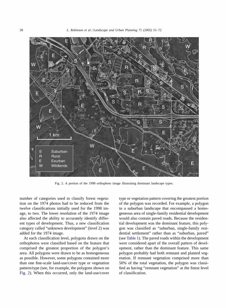
Each polygon was classified based on a hierarchi-cal system (Table 1). First, polygons were viewed ina 1 km2 setting to determine the landscape-level con-text for each polygon. Five categories were used to de-scribe the dominant landscape: urban, suburban, rural,exurban, and wildland. Because of confusion in theliterature over their exact meanings (McIntyre et al.,2000; Marzluff et al., 2001), they were explicitly de-fined for this study (Table 2). A photographic exam-ple of the dominant landscapes defined inTable 2isshown onFig. 2. Note that no areas within the studyarea met the definition of “urban” as defined for this


Table 1Hierarchical land classification system

Dominant landscape (level1)Suburban, rural, or exurban Wildland

Dominant land cover or land-use (level 2)Bare soil

Unpaved gravel roads, or unpaved gravel lots Unpaved gravel roads, or Unpaved gravel lots

PavedMulti-lane/interstate road, or paved road, or

paved lotMulti-lane/interstate road, or paved road, or paved lot

Unknown development(1974 only. No subcategories) (1974 only. No subcategories)

Single-family residential, or multi-familyresidential, or commercial/industrial

<25% vegetation coverage, or 25–75%vegetation coverage, or >75% vegetationcoverage.

Majority clustered vegetation, ormajority dispersed vegetation.

Majority remnant vegetation, ormajority planted vegetation

(Single-family, multi-family, andcommercial/industrial designations notapplicable to wildland areas. See “settlement.”)

Settlement

(“Settlement” used only for wildland areas) Residential only, or Residential/agriculture

Forested vegetation, or forest production area1998 subcategories 1974 subcategories 1998 subcategories 1974 subcategories

Clearcut, or shrub growth/clearcut,or treed vegetation

Treed vegetation,or clearcut/shrubs

Clearcut, or shrubgrowth/clearcut, or treedvegetation

Treed vegetation, orclearcut/shrubs

Non-forest vegetation1998 subcategories 1974 subcategories 1998 subcategories 1974 subcategories

Grasses, or shrubs, or mixed grass/shrub/power corridor

Agriculture, orother non-forestedvegetation

grasses, or shrubs, ormixed grass/shrub/ powercorridor

Agriculture, or othernon-forested vegetation

-or- -or-Lawns: recreational lawns, or golfcourse, or other lawns

Lawns: recreational lawnsgolf course other lawns

-or- -or-Agriculture: croplands, or orchards,or uncultivated fields/pastures

Agriculture: croplands, ororchards, or uncultivatedfields/pastures

Water-related featuresRiver, or lake, or possible wetlands River, or lake, or possible wetlands

Resource use/extraction(“Resource use/extraction” usedonly for wildland areas.)

Logging, or mining, or energy

Polygons were classified by “dominant landscape”, then by “dominant land cover or land-use”. Polygons were further described usingthe categories below to each level 2 designation. For example, an area of single-family homes in a suburban area might be classified as:suburban, single-family residential,<25% vegetation coverage, majority dispersed vegetation, majority planted vegetation. An agriculturalarea might be classified as: rural, non-forest vegetation, agriculture, croplands.


Table 2Definitions of dominant landscape categories

1. Urban: Buildings cover the majority of land. Building density is high and includes multi-family housing, multi-storied buildings,commerce, and industry. High-density single-family housing on relatively small lots (<0.2 ha) is also common. No urban areas wereobserved in the study

2. Suburban: Building density is moderate and lawns and other vegetation are often readily apparent. Lawns and gardens are generallymore extensive than within urban areas. Single-family housing predominates on small to moderately-sized lots (0.1–1.0 ha).Multi-family housing, basic services, and light industry are scattered throughout. Structures over two stories tall are uncommon

3. Rural: Building density is relatively low and surrounded by agricultural lands. Settlement is sparse, primarily single-family housing onmoderate to large lots (0.5–20 ha). For rural lands, we used 30% rather than 50% as the dominant landscape minimum because rural areastend to be long and narrow in shape. Note that the above definition of rural differs from that of King County’s, which define rural landsas any area outside of the urban growth boundaries (UGBs) that are not designated as agriculture or forest production zones (seeFig. 1)

4. Exurban: Building density is relatively low and surrounded by natural vegetation (forests). Average lot sizes are often smaller thanrural (0.2–20 ha). Limited amounts of commercial agriculture may be present, but it does not dominate the matrix. Exurbandevelopment is largely single-family housing carved out of a forest matrix

5. Wildlands: Unsettled, primarily forested, lands that may occasionally include isolated dwellings

To determine dominant landscapes, buildings in each polygon were viewed within a 1 km2 context and assigned to one of the fivecategories listed below. At least 50% of the 1 km2 area was required for a polygon to be labeled a particular dominant landscape. Modifiedfrom Marzluff et al., 2001.

study. Also note that “wildland” is not used in the tra-ditional sense in this study, but is used to denote largetracts (>0.5 km2) of forest lands, with or without ex-tremely light settlement. In this case, wildlands includeprivately-owned managed or unmanaged forests andgovernment-owned parks, forest reserves, and wilder-ness.

Once the dominant landscape was determined, apolygon was then evaluated to determine the dominantland cover at the patch scale (level 2). The level 2 clas-sifications functionally quantify land cover, but some-times used differences in land-use to do so. For exam-ple, polygons were classified by different types of de-velopment (single-family or multi-family residentialdevelopment or commercial development) rather thanby simply defining land cover as “developed,” (i.e.a mixture of impervious surfaces and anthropogenicstructures). These distinctions permitted the quantifi-cation of a fine level of conservation-relevant changesin land cover.

Each polygon was further evaluated to determinethe specific characteristics of land cover (level 3).For example, areas with residential or commer-cial/industrial development, were classified by theamount of vegetative cover (e.g., single-family res-idential settlement with<25% vegetation coverage25–75% coverage, or >75% coverage). These metricsare important when assessing the value of the area as

wildlife habitat. Undeveloped areas with forested andnon-forested vegetation were classified by vegetationtype (e.g., clearcut/shrubs, treed vegetation, or grass).Undeveloped areas in non-vegetated patches that wereobviously not clearcuts (e.g., bare soil, paved) wereclassified by the nature of the land surface (e.g. pavedor unpaved roads or lots;Table 1).

When possible, the specifics of land cover such asvegetation type and pattern were further describedfor each polygon. For example, polygons dominatedby residential and commercial/industrial developmentwere further classified as having clustered or dis-persed vegetation and remnant or planted vegetation(Table 1). Remnant vegetation consists of the natu-ral vegetation left after development while plantedvegetation consists mainly of lawns and landscapeplantings.Classification of the 1974 orthophotos dif-fered slightly from classifications used for 1998. Theclassification system was initially developed based onthe detail we believed could be accurately identifiedon the 1998 orthophotos. For example, at the onsetof the project we believed that we could accuratelydistinguish between different types (coniferous, de-ciduous or mixed forest), ages (young versus mature),and complexity (simple versus complex) of forestvegetation on the 1998 orthophotos. However, theresolution was lower for the 1974 photos and differ-ences between forest types less clear. As a result, the


Fig. 2. A portion of the 1998 orthophoto image illustrating dominant landscape types.

number of categories used to classify forest vegeta-tion on the 1974 photos had to be reduced from thetwelve classifications initially used for the 1998 im-age, to two. The lower resolution of the 1974 imagealso affected the ability to accurately identify differ-ent types of development. Thus, a new classificationcategory called “unknown development” (level 2) wasadded for the 1974 image.

At each classification level, polygons drawn on theorthophotos were classified based on the feature thatcomprised the greatest proportion of the polygon’sarea. All polygons were drawn to be as homogeneousas possible. However, some polygons contained morethan one fine-scale land-use/cover type or vegetationpattern/type (see, for example, the polygons shown onFig. 2). When this occurred, only the land-use/cover

type or vegetation pattern covering the greatest portionof the polygon was recorded. For example, a polygonin a suburban landscape that encompassed a homo-geneous area of single-family residential developmentwould also contain paved roads. Because the residen-tial development was the dominant feature, this poly-gon was classified as “suburban, single-family resi-dential settlement” rather than as “suburban, paved”(seeTable 1). The paved roads within the developmentwere considered apart of the overall pattern of devel-opment, rather than the dominant feature. This samepolygon probably had both remnant and planted veg-etation. If remnant vegetation comprised more than50% of the total vegetation, the polygon was classi-fied as having “remnant vegetation” at the finest levelof classification.


At the start of this project, rules for digitizingand classifying polygons were established to ensureconsistency in classification, such as when to includeroads within a polygon versus when to make roadstheir own polygon, or how to distinguish “bare soil”from a recent “clearcut.” To ensure accuracy andconsistency in interpreting the orthophotos, a trainingsession was held in the study area to jointly practicethe assignment of classification codes.

Periodic ground-truthing was used to verify the ac-curacy of assigned classification codes (for the 1998image) and to resolve questions and concerns thatarose during the digitizing process. When inconsisten-cies were discovered, classification codes were mod-ified to reflect actual conditions. Approximately 25%of the study area was ground-truthed during the clas-sification process.

Questions and concerns regarding the 1974 or-thophotos were more difficult to deal with. Ques-tionable areas were compared to the 1998 imagefor clarification. For example, a fuzzy area on the1974 orthophoto that appeared to be devoid of veg-etation and possibly developed might show up as awell-established forest stand on the 1998 image, in-dicating that it was most likely a clearcut in 1974.Where questions could not be resolved, the polygonwas classified as unknown development.

The consistency of codes assigned during the clas-sification process was tested partway through thedigitizing process. Three of the five digitizers did 40sample trials to assess the team’s consistency. Therewere some inconsistencies. For example, dominantlandscape (level 1) was inconsistently classified 18%of the time and land-use/cover (level 2) was incon-sistently classified 5% of the time. To correct this,the entire team reviewed the definitions for dominantlandscape (Table 2) and rules for digitizing. Each per-son then reviewed their portion of the study area andmade changes as needed. In sections of the orthopho-tos where classification was difficult, team membersworked together. Polygons on the 1998 image thatwere difficult to classify were later ground-truthed.

Consistency tests also showed that fine-scale dis-tinctions for forest vegetation (e.g., deciduous versusconiferous forest, various forest ages) were incon-sistently classified 23% of the time. Ground-truthingalso showed that forest vegetation was inaccuratelyclassified much of the time. As a result, the fine-scale

distinctions for forests initially used for the 1998 pe-riod were combined into a few classifications (e.g.treed vegetation) prior to analysis (Table 1).

2.4. Calculating interior forest habitat and edge

Interior forest area and edge density were calcu-lated for wildland landscapes using patch analyst(Rempel et al., 1999), assuming a buffer of 200 mto account for edge effects (Kremsater and Bunnell,1999). Edge density, a measure of edge in relation tototal area, was calculated by dividing total edge bytotal area. Interior forest area was also calculated forfragments of clustered/remnant forest in areas dom-inated by single-family housing in suburban, rural,and exurban landscapes. Using 200 m for the extentof edge effects, each patch of vegetation classifiedas clustered/remnant (>75% vegetative cover) in apolygon dominated by single-family housing wasmeasured using arc view’s measurement tool to de-termine if the fragment had any area that was >200 mfrom settlement.

2.5. Patch analysis

The distribution of single-family housing and veg-etative cover between the two study years was com-pared using a chi-square (χ2) goodness-of-fit test. Thenumber of patches of single-family housing or vege-tative cover class (>25, 25–75, and >75%) were com-pared among dominant landscape classes (suburban,rural, exurban), also using the chi-square test. Meanpatch size for each class of dominant landscape wasalso compared between study years using an indepen-dent samplest-test. Because the variance increasedwith the mean, all patch data was log-transformedprior to analysis (Zar, 1999).

2.6. Assessing the effects of changing policies

Growth management policies governing land-useand development in the study area changed signifi-cantly during the study period. Such policy changescan result in a noticeable change in housing devel-opment patterns around the time the new programsare implemented. Changes in patterns often start be-fore new policies are enacted. For example, in the


years just prior to adoption of the King County’s1985 comprehensive plan, there was a rush to subdi-vide larger parcels to “grandfather in” smaller parcelsbefore lot sizes for buildable parcels increased (Re-itenbach, Personal Communication). The effects of“grandfathering” could continue for up to several yearsafter a new policy is enacted.

While the analysis of intermediate orthophotos (be-tween 1974 and 1998) could reveal changes in landdevelopment patterns resulting from policy changes,it was unclear which years should be investigated. Inaddition, orthophotos were not available for many ofthe intervening years. Thus, external data sources weredeemed superior than additional photo interpretationfor determining the effects of these changes on thedistribution of housing within the study area. Resi-dential housing parcel data fromKing County (2002),which provides information about permits issued forconstruction of single-family residences county-wide,was analyzed for number of permits and amount ofland developed on a year-by-year basis to look forchanges in the pattern of residential land development,both inside and outside UGBs.

3. Results

3.1. Amount and pattern of change

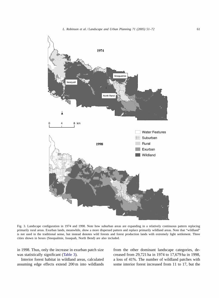
Suburban and exurban landscapes increased be-tween 1974 and 1998 (Fig. 3). In 1974, suburban

Table 3Patch size of dominant landscape categories

Category Number of patches Total area (ha) Mean patch size (ha)

1974 1998 1974 1998 Percentchange(%)

1974 Standarderror(1974)

1998 Standarderror(1998)

Percentchange(%)

t P

Suburban 9 14 668 5720+756 74 43 409 319 +453 −1.121 0.275Rural 74 34 6181 2176 −65 84 45 64 21 −24 −1.543 0.126Exurban 77 62 3102 9090 193 40 19 147 74 +268 −2.835 0.005Wildland 42 48 35437 28687 −19 844 711 598 405 −29 0.574 0.568Water – – 1995 1730 – – – – – – – –

Total 47383 47403

A patch is defined as a contiguous area of homogeneous classification. Total patch size is the total area of a given landscape category andaverage patch size is the average based on total area divided by the total number of patches for a given landscape category for a givenyear. Percent change is based on the percent increase or decrease in area from 1974 to 1998. Tests of change in mean patch size are basedon log-transformed data. Note that total areas of water features vary for each study year due to differences in digitizing their boundaries.

and exurban lands together comprised just 8% of thestudy area, but by 1998 they covered almost a third.Suburban land increased by 756% and exurban landby 193% (Table 3). At the same time, rural landsdecreased by 65% and wildlands by about 19%. Con-sidering that in 1974 wildlands accounted for about75% of the study area, this 19% decrease represents asubstantial area (about 68 km2). Together, the reduc-tion of rural and wildland areas represent the conver-sion of 23% of the study area (about 108 km2) fromnatural resource and agricultural production lands toresidential and commercial development. Land thatwas suburban in 1974 generally remained suburban in1998 (Table 4). However, only 19% of lands classifiedas rural in 1974 remained rural in 1998. Sixty-onepercent of rural lands in 1974 became suburban by1998, and 18% became exurban. Similarly, 19% ofsuburban lands and 17% of wildlands became exurbanby 1998.

Settled lands became more contiguous during the24-year study period, while fragmentation increasedelsewhere (Fig. 4, Table 3). Mean patch size of subur-ban and exurban lands increased by 453% and 268%,respectively. This constitutes infilling between Seat-tle and the once-isolated fringe communities of Is-saquah, Snoqualmie, and North Bend (Fig. 3). At thesame time, mean patch size for rural and wildlandsdecreased, indicating increased fragmentation (Figs. 4and 5). In addition to large differences in mean patchsize between 1974 and 1998 for all landscape cate-gories, there was also a large variance in patch size


Fig. 3. Landscape configuration in 1974 and 1998. Note how suburban areas are expanding in a relatively continuous pattern replacingprimarily rural areas. Exurban lands, meanwhile, show a more dispersed pattern and replace primarily wildland areas. Note that “wildland”is not used in the traditional sense, but instead denotes wild forests and forest production lands with extremely light settlement. Threecities shown in boxes (Snoqualmie, Issaquah, North Bend) are also included.

in 1998. Thus, only the increase in exurban patch sizewas statistically significant (Table 3).

Interior forest habitat in wildland areas, calculatedassuming edge effects extend 200 m into wildlands

from the other dominant landscape categories, de-creased from 29,721 ha in 1974 to 17,679 ha in 1998,a loss of 41%. The number of wildland patches withsome interior forest increased from 11 to 17, but the


Table 4Percent change in dominant landscape from 1974 to 1998

Dominant landscape 1974 Dominant landscape 1998 Land area changed (ha) Percent change from 1974 to 1998

Suburban Suburban 661a 92Suburban Rural 4 1Suburban Exurban 47 7Suburban Wildlands 5 1

Rural Suburban 3304 54Rural Rural 1780a 29Rural Exurban 880 14Rural Wildlands 1873

Exurban Suburban 688 22Exurban Rural 16 1Exurban Exurban 2373a 77Exurban Wildlands 21 1

Wildlands Suburban 1054 3Wildlands Rural 240 1Wildlands Exurban 5733 16Wildlands Wildlands 28340a 80

Total 45282

a Note that each category shows the amount of land that did not change. Note also that water features are excluded from this analysis.

average size of these areas declined by 61%, from2701 to 1040 ha. Total edge (measured as the lengthof interface between wildland and other dominantlandscape categories) decreased by 29%, from 913to 644 km. This decrease in edge reflects the overalldecrease in size of core areas. Edge density, a mea-sure of edge in relation to total area, increased from30 m/ha in 1974 to 36 m/ha in 1998.

In 1998, the amount of vegetative cover withinsingle-family residential areas varied significantly(χ2 = 45.3, d.f . = 4, P < 0.05). Not surprisingly, theamount of vegetative cover within single-family hous-ing developments was higher in rural and exurbanareas than in suburban areas (Table 5). Eighty percent

Table 5Vegetation cover in single-family housing developments, 1998

Category <25% 25–75% >75%

Area (ha) % Area (ha) % Area (ha) %

Suburban 678.9 24 1090.7 39 1012.2 36Rural 15.5 4 66.7 16 332.5 80Exurban 15.5 <1 341.9 7 4422.5 92Total 709.9 9 1499.3 19 5767.2 72

Single-family housing in rural and exurban areas are highly veg-etated (>75%), while those in surburban areas have a mix of low(<25%), medium (25–75%) and high (>75%) levels of vegetation.

of the area covered by rural single-family housingand 92% in exurban single-family housing areas had>75% vegetative cover, but only 36% of suburbansingle-family residential areas had that much vegeta-tion. In contrast, less than 5% of rural and exurbansingle-family residential areas had<25% vegetativecover, compared to 24% of suburban residential areas(Table 5).

Vegetation in single-family housing developmentswas highly fragmented and the remaining fragmentswere frequently isolated with little connectivity(Fig. 5). In general, vegetation across all patches dom-inated by single-family development was dispersed(76%) rather than clustered (24%). In suburban andrural lands, much of the vegetation was planted (42and 57%, respectively), not remnant. However, inexurban lands, remnant vegetation was dominant in94% of all housing developments. Some develop-ments had substantial fragments of clustered/remnantvegetation (Table 6). However, these fragments weremostly elongated (rather than compact), with a highedge/interior ratio. Even when adjacent fragmentsin areas dominated by single-family housing couldbe combined to form large patches, no patches hadany area >200 m from the edge, and only one patchcontained any area at a distance >100 m from an edge.

L.

Ro

bin

son

et

al./L

an

dsca

pe

an

dU

rba

nP

lan

nin

g7

1(2

00

5)

51

–7

263

Fig. 4. Changes within each category of dominant landscape, 1974–1998. Each map shows change in dominant landscape (suburban, exurban, rural, and wildland) from1974–1998. Note that suburban and exurban areas are increasing over time while rural and wildland (wild forests and forest production lands with light settlement) aredecreasing. These are the same data contained inFig. 2, but presented here to clearly show changes within each type of landscape.

64L

.R

ob

inso

ne

ta

l./La

nd

scap

ea

nd

Urb

an

Pla

nn

ing

71

(20

05

)5

1–

72

Fig. 5. Distribution of vegetation, 1974 and 1998; (a) and (b) show changes in vegetative cover; (c) shows vegetation patterns in single-family housing for 1998. No parksare shown for 1974.


Table 6Total area with clustered/remnant vegetation

Category <25% vegetation 25–75% vegetation >75% vegetation Total

Suburban area (ha) 70.2 (1) 214.1 (5) 173.3 (8) 457.6 (14)Percent of total (%) 4 12 10 26

Rural area (ha) 0 30.1 (1) 18.3 (1) 48.4 (2)Percent of total (%) 0 2 1 3

Exurban area (ha) 0 109.6 (3) 1137.4 (17) 1247.0 (20)Percent of total (%) 0 6 65 71

Total Area (ha) 70.2 (1) 353.8 (9) 1329.0 (26) 1753 (36)Percent of total (%) 4 20 76 100

Areas are totals by dominant landscape categories. Numbers in parentheses are number of patches.

There were approximately 271 more hectare ofsurface water in the study area in 1974 than in 1998.About 112 ha of the difference are due to the loss ofsurface water bodies to filling and development alongshorelines. For example, three areas east of Sno-qualmie that total about 60 ha were ponds in 1974,but agricultural fields in 1998 (Fig. 5). The pres-ence of these agricultural fields in 1998 was verifiedby ground-truthing. The remainder of the difference(159 ha; 0.3% of the study area) appeared to be due toslight differences in digitizing rivers and lakes in thetwo study years. Because the 1998 image had a muchhigher resolution than the 1974 image, the shorelinesof rivers and lakes were digitized much more tightlyand accurately than for 1974. In general, polygonsdrawn for rivers and lakes were broader for 1974 thanfor 1998.

3.2. Expansion of low-density, single-family housing

Single-family housing was a primary cause ofland conversion. Expansion of single-family housing(Fig. 6) closely resembles the overall pattern of landconversion (Figs. 3 and 4). There were significantlymore patches of single-family housing in suburbanand exurban areas in 1998 than in 1974 (χ2 = 44.72,d.f . = 3, P < 0.001), while the number of patches ofsingle-family housing in areas now classified as ruraland wildland remained relatively constant. However,most single-family development since 1974 has takenplace in former wildland areas that are now classifiedas exurban. Conversion to commercial developmentwas more frequent in already settled areas.

Total land developed for residential housing andcommercial uses within the study area increased by134%, from 3842 ha in 1974 to 8994 ha in 1998. Ineach study year, about 88% (3380 and 7976 ha, respec-tively) of developed land consisted of single-familyhousing. The percent of land devoted to commer-cial development also stayed relatively constant(12 and 10%, or 463 and 895 ha, respectively). Nomulti-family housing was observed in 1974, and only1.4% (123 ha) of all developed land in the study areawas classified as multi-family in 1998. It is importantto note, however, that 1108 ha of developed areaswere classified as “unknown development” in 1974due to poor image resolution (Fig. 6). Comparison ofthese unknown areas to the same locations in 1998showed that they were most likely to have been ei-ther single-family housing in 1974 or clearcuts laterdeveloped for single-family housing. As a result, theywere grouped with single-family housing during anal-ysis of 1974 data. Because of this uncertainty, how-ever, the amount of single-family housing is likelyoverstated in 1974 and multi-family and commercialdevelopment may be understated.

3.3. Relationship between development patternsand policy changes

There was considerable expansion of low-densitysingle-family housing outside the UGBs between1974 and 1998 (Fig. 6). Although some of the de-velopment outside the UGBs occurred before theUGBs were established in 1994, residential housingparcel data fromKing County (2002)showed that


Fig. 6. Expansion of single-family housing within rural, exurban, and suburban landscapes, 1974–1998. For data analysis, unknowndevelopment is grouped with single-family housing in 1974.

a substantial portion occurred after the UGBs wereestablished (Fig. 7; Table 7). However, based on ayear-by-year analysis of residential building permitsissued for the study area between 1974 and 2001,there was no clear pattern of development of rural

areas related to implementation of either the 1985 or1994 King County comprehensive plans. The correla-tion between study year and the number of residentialbuilding permits issued was weak (Spearman’s rankcorrelation,r = 0.13, n = 28, P = 0.51).


Fig. 7. Expansion, in land area, of residential housing outside of the urban growth boundaries (UGBs). Growth derived from King Countyresidential parcel data, 1994–2001.

County parcel data showed that most of the resi-dential building permits (77%) issued from 1995 to1998 (following implementation of the 1994 compre-hensive plan) were for parcels inside the UGBs, indi-cating that building density increased within existingurban areas. However, the increase in the percent ofresidential building permits issued within urban ar-eas since establishment of the UGBs (1994) is ratherslight (Table 7). From 1995 to 1998, 60% of landpermitted for new residential development withinthe study area occurred outside the UGBs (Table 7).Thus, the total land area newly devoted to housingis much greater outside the urban growth bound-aries, despite the relatively low number of residentialbuilding permits issued for those areas. These sametrends continued through 2001 and are consistentwith residential housing development county-wide.For example, parcel data for 1997 to 2001 show thatcounty-wide, 14% of new residential building per-mits (5494) were issued for parcels outside UGBs,yet total land area developed for residential housingoutside the UGBs was 61%. County-wide, a total of14343 ha (61%) were committed to new residentialconstruction outside UGBs, while 9084 ha (39%) of

land was developed within UGBs from 1995 to 2001(King County, 2002).

4. Discussion

4.1. Ecological effects of low-density development inKing County

King County’s growth management policies havetargeted rural and wildland areas outside designatedurban growth boundaries for low-density residen-tial development, ostensibly to maintain rural char-acter and protect the natural environment of theseareas while still allowing some development to oc-cur (KCORPP, 2000b). King County is not alone inusing low-density development as a means to limitimpacts to rural areas. Decreasing the density of res-idential housing, also known as “downzoning,” hasbeen used by many local governments, in an effortto maintain community character, create open space,and protect the environment (Gillham, 2002). How-ever, asGillham (2002)points out, downzoning is notnecessarily an effective method for preserving rural


Tabl

e7

Dis

trib

utio

nof

build

ing

perm

itsan

dla

ndco

mm

itted

toco

nstr

uctio

nof

resi

dent

ial

hous

ing

with

inst

udy

area

1974

–198

419

85–1

994

1995

–199

819

99–2

001

Land

com

mitt

edB

uild

ing

perm

itsLa

ndco

mm

itted

Bui

ldin

gpe

rmits

Land

com

mitt

edB

uild

ing

perm

itsLa

ndco

mm

itted

Bui

ldin

gpe

rmits

Loca

tion

Are

a(h

a)%

Tota

l%

Are

a(h

a)%

Tota

l%

Are

a(h

a)%

Tota

l%

Are

a(h

a)%

Tota

l%

Insi

deU

GB

1357

3530

0062

1638

2849

0172

1108

4021

5277

323

1517

7679

Out

side

UG

B25

5665

1874

3842

6872

1836

2817

3660

651

2318

2585

474

21

Tota

l39

1348

7459

0667

3728

8428

0321

4822

50

Tim

epe

riods

rela

teto

maj

orch

ange

sin

grow

thm

anag

emen

tpo

licie

s(e

.g.

the

1985

and

1994

Kin

gC

ount

yC

ompr

ehen

sive

Pla

ns),

exce

ptfo

r19

98–2

000,

wh

ich

refe

rsto

the

chan

ges

sinc

eth

e19

98or

thop

hoto

.D

ata

fromKin

gC

ount

y(2

002).

character or protecting the environment; additionalhouses are still constructed and undeveloped landis still subdivided into smaller parcels, all of whichresult in adverse environmental impacts, loss of openspace, and increased traffic and infrastructure costs.

As shown by this study, the policy of low-densityzoning has had unintended consequences. Despitethe apparent increase in density of existing urban ar-eas, this zoning policy has resulted in wide-spread,low-density single-family residential developmentoutside the UGBs in the study area, resulting in sub-stantial loss of rural areas and wildlands to suburbanand exurban development. This has clearly had a ma-jor impact on landcover in the study area—converting,fragmenting, and isolating forest and rural lands. Na-tive forest understories have been replaced with exotic,planted landscapes. The pattern of housing seen inexurban portions of the study area, dispersed through-out what were formerly rural areas and wildland, hasnoticeably reduced interior forest habitat. The fewfragments of clustered/remnant vegetation present inpatches dominated by single-family housing were toosmall to include interior habitat; just one patch hadforest >100 m from its interface with developed land.Some patches without interior habitat were adjacentto parklands and working forests (Fig. 5), increasingthe possibility of interior conditions. However, manyof these working forests are themselves fragmentedby roads and logging activities, which increase thepotential for human impacts (Rochelle et al., 1999).For example, in his study of suburban forest frag-ments in Delaware,Matlack (1993)showed that sitesadjacent to roads were significantly more affectedby human activities than those away from vehicleaccess.

Fragmentation of once contiguous forests can po-tentially affect many sensitive species that requireinterior forest conditions. Species that would be neg-atively affected by this change in our area includethe federally threatened Northern Spotted Owl (Strixoccidentalis) and Marbled Murrelet (Brachyram-phus marmoratus), neotropical migrant birds such asthe Wilson’s Warbler (Wilsonia pusilla), and sensi-tive resident species like Winter Wrens (Troglodytestroglodytes), spotted frogs (Rana pretiosa), Pacificgiant salamanders (Dicamptodon tenebrus), duskyand Trowbridge shrews (Sorex monticolusand S.trowbridgii), and shrew-moles (Neurotrichus gibbsii).


Broadly applied low-density zoning policies need tobe refined to reduce sprawl, fragmentation, and habi-tat loss. Rather than zoning all areas outside of UGBsfor low-density residential development, King Countyand other local governments should consider zoning atleast some of these areas at a variety of higher densi-ties while limiting the overall number of dwelling unitsthat could be constructed in a given area. In addition,some areas should also be zoned for clustered devel-opment. Clustering allows some land to be set aside asopen space, helping to preserve rural character whilereducing habitat loss, environmental impacts and in-frastructure costs (Gillham, 2002). Within a given area,some parcels should be zoned for clustered develop-ment while others should be zoned for no develop-ment. In this model, the overall number of residentialstructures would remain the same, but much less landwould be consumed. As an example, if rural residen-tial lot sizes were reduced from 2–8 ha (5–20 acres) to1 ha (2.5 acres; still a relatively large lot), and if theseresidential parcels were clustered, then a substantialamount of land would remain undeveloped and possi-bly even able to provide interior forest conditions. Ifthis had been done in the study area, the amount ofland consumed by the 1125 residential structures con-structed outside UGBs between 1994 and 2001 wouldhave been reduced from 8905 to 2813 acres, a reduc-tion of 68%. This would have greatly decreased thefragmentation of forests and losses of interior forestdocumented by this study.

King County has taken some steps to encourage pro-tection of significant habitats and other critical areasin rural and exurban areas, including buffering sen-sitive watercourses, creating interior forest reserves,protecting rare habitat elements (dead and downedtrees, native understory, seeps, etc.), and maintain-ing key ecosystem processes (decay, natural distur-bance regimes including fire, etc.). However, designa-tion of long-term forest and agriculture production ar-eas has had the most beneficial impact in terms of thebroader landscape-level conservation of environmen-tal resources in the county. As shown inFig. 1, morethan half the county has received these long-term des-ignations; this has strongly limited the spatial extentof future growth. In these production areas, land hasto remain in large parcels, the priority land-use is foragriculture or forest production, and there are stronglimitations on development (King County, 1994). With

these designations, the county has effectively createdthree development zones: urban growth areas, lowerdensity rural areas, and forest and agriculture produc-tion areas (seeFig. 1). Thus, while we see sprawloccurring within the study area, the future extent ofsprawl has been effectively limited by designation ofthe forest and agriculture production areas as well asthe proximity of large state and federal land holdings.

This foresight by King County should not be un-derestimated. At present, more than 250,000 acresof King County’s forest production lands are in pri-vate ownership (KCORPP, 2001), with the remain-der consisting of large blocks of federal, state, orcounty-owned land. Most of the privately held landsare adjacent to the rural areas slated for low-densitydevelopment. Given the amount of privately-ownedforest production land, it is likely that some of theseareas would have already been developed withoutthese long-term designations, thereby increasing theextent of sprawl. Although little new residential con-struction is supposed to occur in these areas, they arealready under pressure for a greater level of develop-ment (The Seattle Times, 2000).

4.2. Applicability and generalizability

The results from this study indicate that aerialphotographs (orthophotos) are an accurate means todocument and analyze land-use/land cover changesand patterns in urbanizing areas. When used withcomputer-based GIS programs, high-quality orthopho-tos provide a level of landscape detail not achievablewith remote sensing. Aside from the scale resolutionlimit of about 7000:1, the primary limiting factor isthe ability of classifiers to accurately and consistentlyidentify the details shown on the photo. This can beovercome through the use of strict rules for digitizingand classifying, and training sessions. The classifica-tion system used to describe land cover/land-use inthe study area can also be a limiting factor if the needsand objectives of the study are not well thought outbefore beginning the digitizing process. The need forconstant communication between classifiers and theneed for ground-truthing throughout the classificationprocess became readily apparent during the courseof this study. Periodic tests of consistency betweenclassifiers are also necessary to ensure that the datagenerated are reliable.


With these measures in place, use of orthophotos,the classification system, and method are recommendfor those researching the heterogeneous, dynamiclandscapes found in urbanizing areas in other geo-graphic regions. For example, using high-resolutionorthophotos coupled with an appropriate classificationsystem would add valuable ground-level detail to ananalysis of land cover/land-use changes, such as theon-going studies being conducted in Russia using acombination of satellite imagery and historical maps(Milanova et al., 1999). Similarly, an orthophotostudy could add detail to an analysis of the pattern ofresidential construction found in areas where govern-ment policies limit construction, such as in the “GreenHeart” area of the Netherlands (Tjallingii, 2000).

The habitat fragmentation and loss of interior habi-tats documented by this study are generalizable togeographic areas throughout the world experiencingrapid growth and sprawling, low-density development.This is wide-spread throughout the Western US, whereexurban and rural settlement is common throughoutprivately held lands (Hansen et al., 2002). Fragmen-tation of forests, open space, and agricultural lands isalso a frequently-discussed impact in other countriesincluding The Netherlands (Valk, 2002) and Japan(Sorensen, 1999). The spatial extent of low-densitysettlement is likely unique to each region and setby a combination of settlement policies. WashingtonState, for example, has strong growth managementpolicies that have slowed moderate- to high-densitysettlement beyond county-defined UGBs. However,even such legally-mandated growth management ap-pears unable to truly limit lower density settlementin privately-owned agricultural and forested landsbeyond urban growth boundaries. For example, thisstudy showed in that in King County, 61% of landcommitted for residential construction between 1995and 2001 took place outside designated urban growthboundaries. Similarly, “compact city” policies thatencourage construction of new residential develop-ment within existing urban centers, coupled with re-strictive land development policies for the rural greenheart area of The Netherlands, have not been entirelysuccessful.Tjallingii (2000) noted that a substantialportion of new residential construction is still occur-ring within the restricted green heart area, including43% of new housing between 1989 and 1994. In KingCounty, local geology, land ownership, and zoning

interact to stop settlement in high-elevation federaland state lands that are currently zoned for resourceproduction and recreation. In other settings, lands re-served from settlement may not exist in proximity tosprawling urban centers and therefore more extensivelow- to high-density settlement is likely depending onthe existence of local growth management policies.

5. Conclusions

Policies encouraging dispersed, low-density devel-opment in rural and wildland areas have clear impli-cations for planners and biologists. This paper showedthat scattered, low-density housing consumes naturalhabitat, in much greater quantities than if housingwere predominantly constructed at higher densitiesin more compact developments (Gillham, 2002). Theunintended consequence—the increasing loss, frag-mentation, and isolation of natural habitats—is theopposite of what these policies were intended to ac-complish: conserve fish and wildlife habitat, protectand enhance the environment, while still allowingsome residential development to take place (KCORPP,2000b). The power of designating long-term naturalresource and agriculture production areas, in combi-nation with policies that encourage increased densityof urban areas and limit growth in more rural areas,is also clearly indicated. Without these long-termdesignations, sprawling, low-density developmentwould likely become more wide-spread throughoutthe county, increasing habitat fragmentation whiledecreasing the amount of interior habitat available towildlife species. The designated forest and agricultureproductions lands act as a barrier, effectively limitingthe spread of new residential development away fromurban areas.

As human populations become increasingly urban,without policy changes to control it, sprawl will be-come even more wide-spread than at present. In theyear 2000, about 3 billion people (50% of the world’spopulation) lived in urban areas and this figure is ex-pected to reach 5 billion by 2025 (UNU/IAS, 2003).Countries enacting growth management policies tocontrol sprawl should be wary of using low-densityzoning to limit development in the more rural areasoutside urban centers. As this study showed, usinglow-density zoning to restrict development may have


unintended consequences and may in fact encouragesprawl.

Acknowledgements

This project was developed as part of the interdis-ciplinary Urban Ecology Program at the University ofWashington. Graduate Students, Undergraduates, andFaculty from the College of Forest Resources, Ge-ography Department, School of International Studies,and Urban Design and Planning Department workedtogether to define a problem related to land conver-sion at the urban fringe, then to develop a researchprogram to address it. Cathy Lander, Colleen Srull,and Sasha Sajovic helped develop the project and theLand Classification System, and put in long hoursdigitizing orthophotos. Tina Rohila, Alex Cohen, andDana Morawitz worked on the remote sensing portionof this project and provided valuable input and as-sistance. Eric Shulenberger, Clare Ryan, Craig Zum-Brunnen, Gordon Bradley, and Marina Alberti pro-vided guidance and critically reviewed all aspects ofthe project. Phil Hurvitz taught us the basics of GIS.We also wish to thank Washington Department of Nat-ural Resources for providing the aerial orthophotos,and King County for the use of their GIS database.Funding was provided by the US National ScienceFoundation (IGERT-0114351) and the University ofWashington’s Tools for Transformation program ad-ministered by Debra Freidman. We also wish to thankthe anonymous reviewers of our manuscript, whosecomments greatly improved our paper.

References

Alberti, M., Marzluff, J.M., Shulenberger, E., Bradley, G., Ryan,C., Zumbrunnen, C., 2003. Integrating humans into ecology:opportunities and challenges for studying urban ecosystems.Bioscience 52 (12), 1169–1179.

Benfield, F.K., Raimi, M.D., Chen, D.D.T., 1999. Once therewere greenfields: how urban sprawl is undermining America’senvironment, economy, and social fabric. Natural ResourcesDefense Council, Washington, DC.

Breheny, M., 1995. Counter-urbanisation and sustainable urbanforms, 1995. In: Brotchie, J., Batty, M., Blakely, E. et al. (Eds.),Cities in competition: productive and sustainable cities for the21st century. Melbourne, Longman, Australia.

Bullard, R.D., Johnson, G.S., Torres, A.O., 2000. Sprawl city: race,politics, and planning in Atlanta. Island Press, Washington, DC.

Cadenasso, M.L., Pickett, S.T.A., 2001. Effect of edge structureon the flux of species into forest interiors. Conservation Biol.15, 91–97.

Ewing, R., 1997. Is Los Angeles-style sprawl desirable? J. Am.Plan. Assoc. 63, 107–127.

ERDAS, 2002. ERDAS Macro Language Reference Manual.ERDAS IMAGINE V8.6. Inc. Atlanta, Georgia.

Gillham, O., 2002. The Limitless City: A Primer on the UrbanSprawl Debate. Island Press, Washington, DC.

Hansen, A.J., Rasker, R., Maxwell, B., Rotella, J.J., Wright, A.,Langner, U., Cohen, W., Lawrence, R., Johnson, J., 2002.Ecology and socioeconomics in the New West: a case studyfrom greater yellowstone. BioScience 52, 151–168.

Ioffe, G., Nefedova, T., 1998. Environs of Russian cities: a casestudy of Moscow. Europe-Asia Studies 50, 1325–1356.

Ioffe, G., Nefedova, T., 2001. Land-use changes in the environsof Moscow. Area 33, 273–286.

KCDPCD (King County Department of Planning and CommunityDevelopment), 1985. King County Comprehensive Plan. KingCounty, Washington.

King County, 1994. King County Comprehensive Plan. KingCounty Department of Development and EnvironmentalServices, King County, Washington.

King County, 2002. King County Spatial Data Catalog: Zoning.King County GIS Center, King County, Washington.

KCORPP (King County Office of Regional Policy and Planning),2000a. The Annual Growth Report 2000. King County,Washington.

KCORPP (King County Office of Regional and Policy Planning),2000b. King County County-Wide Planning Policies. KingCounty, Washington.

KCORPP (King County Office of Regional Policy and Planning),2001. King County Comprehensive Plan 2000. Adopted 12February 2001. King County, Washington.

KCORPP (King County Office of Regional Policy and Planning),2002. King County County-wide Planning Policies. UpdatedNovember 2002. King County, Washington.

Kremsater, L., Bunnell, F.L., 1999. Edge effects: theory, evidenceand Implicaitions to management of Western North Americanforests. In: Rochelle, J.A., Lehmann, L.A., Wisniewski,J. (Eds.), Forest Fragmentation: Wildlife and ManagementImplications. Koninklijke Brill NV, Leiden, The Netherlands.

Marzluff, J.M., 2001. Worldwide urbanization and its effect onbirds. In: Marzluff, J., Bowman, M., Donnelly, R., (Eds.), AvianEcology and Conservation in an Urbanizing World. KluwerAcademic Publishers, Boston, Massachusetts.

Marzluff, J.M., Restani, M., 1999. The effects of forestfragmentation on avian nest predation. In: Rochelle, J.A.,Lehmann, L.A., Wisniewski, J. (Eds.), Forest Fragmentation:Wildlife and Management Implications. Koninklijke Brill NV,Leiden, The Netherlands.

Marzluff, J.M., Bowman, M., Donnelly, R., 2001. A historicalperspective on urban bird research: trends, terms, andapproaches. In: Marzluff, J.M., Bowman, M., Donnelly R.(Eds.), 2001. Avian Ecology and Conservation in an UrbanizingWorld. Kluwer Academic Publishers, Boston, Massachusetts.


Matlack, G.R., 1993. Sociological edge effects: spatial distributionof human impact in suburban forest fragments. Environ. Manag.17, 829–835.

McDonnell, M.J., Pickett, S.T.A., Groffman, P., Bohlen, P., Pouyat,R.V., Zipperer, W.C., Parmelee, R.W., Carreiro, M.M., Medley,K., 1997. Ecosystem processes along an urban-to-rural gradient.Urban Ecosystems 1, 21–36.

McIntyre, N.E., Knowles-Yanez, K., Hope, D., 2000. Urbanecology as an interdisciplinary field: differences in the useof “urban” between the social and natural sciences. UrbanEcosystems 4, 5–24.

McKinney, M.L., 2002. Urbanization, biodiversity, and conserva-tion. BioScience 52, 883–890.

Milanova, E.V., Lioubimtseva, P.A., Tcherkashin, P.A., Yanvareva,L.F., 1999. Land-use/cover change in Russia: mapping and GIS.Land-use Policy 16, 153–159.

O’Meara, M., 1999. Reinventing cities for people and the planet.Worldwatch Paper 147. Worldwatch Institute, Washington, DC.

Porter, D., 1997. Managing Growth in America’s Communities.Island Press, Washington, DC.

Razin, R., 1998. Policies to control urban sprawl: planningregulations or changes in the ‘rules of the game’? Urban Stud.35, 312–340.

Rempel, R.S., Carr, A., Elkie, P., 1999. Patch analyst andpatch analyst (grid) function reference. (http://www.lakeheadu.ca/∼rrempel/patch/). Centre for Northern Forest EcosystemResearch, Ontario Ministry of Natural Resources, LakeheadUniversity, Thunder Bay, Ontario, Canada.

Rochelle, J.A., Lehmann, L.A., Wisniewski, J. (Eds.), 1999.Forest Fragmentation: Wildlife and Management Implications.Koninklijke Brill NV, Leiden, The Netherlands.

Rothblatt, D.N., 1994. North American metropolitan planning,Canadian and US perspectives. J. Am. Plan. Assoc. 60, 501–520.

Sorensen, A., 1999. Land readjustment, urban planning, and urbansprawl in the Tokyo metropolitan area. Urban Stud. 36, 2333–2360.

The Seattle Times, 2000. County tries to slow sprawl into ruralareas. 19 January 2000.

Tjallingii, S.P., 2000. Ecology on the edge: landscape and ecologybetween town and country. Landscape Urban Plan. 48, 103–119.

UNU/IAS (United Nations University/Institute of AdvancedStudies, 2003. Urban Ecosystem Analysis: Identifying Toolsand Methods. Jingumae, Shibuya-ku, Tokyo.

US Fish and Wildlife Service, 2000. Status and Trends of Wetlandsin the Conterminous United States 1986 to 1997. Washington,DC.

Valk, van der A., 2002. The Dutch planning experience. LandscapeUrban Plan. 58, 201–210.

Vitousek, P.M., Mooney, H.A., Lubchenco, J., Melillo, J.M., 1997.Human domination of Earth’s ecosystems. Science 277, 494–499.

Wu, F.L., Yeh, A., 1997. Changing spatial distribution anddeterminants of land development in Chinese cities in thetransition from a centrally planned economy to a socialistmarket economy: a case study of Guangzhou. Urban Stud. 34,1851–1879.

Zar, J.H., 1999. Biostatistical Analysis, Fourth ed. Prentice Hall,Upper Saddle River, New Jersey.

Zuidema, P.A., Sayer, J.A., Dijkman, W., 1996. Forestfragmentation and biodiversity: the case for intermediate-sizedconservation areas. Environ. Conservation 23, 290–297.

http://www.lakeheadu.ca/~rrempel/patch/

http://www.lakeheadu.ca/~rrempel/patch/

Documents

Twenty-ﬁve years of sprawl in the Seattle region: growth ...urbansustainability.snre.umich.edu/wp-content/uploads/...Landscape and Urban Planning 71 (2005) 51–72 Twenty-ﬁve years