TVL1 Shape Approximation from Scattered 3D Data

E. Funk1,2, L. S. Dooley1 and A. Boerner2

1 Department of Computing and Communications, The Open University, Milton Keynes, United Kingdom2Department of Information Processing for Optical Systems, Institute of Optical Sensor Systems, German Aerospace

Center, Berlin, Germanyl.s.dooley@open.ac.uk, {eugen.funk, anko.boerner}@dlr.de

Keywords: Shape Reconstruction, Radial Basis Function Interpolation, L1 Total Variation Minimization, Iterative LargeScale Optimization

Abstract: With the emergence in 3D sensors such as laser scanners and 3D reconstruction from cameras, large 3D pointclouds can now be sampled from physical objects within a scene. The raw 3D samples delivered by thesesensors however, contain only a limite d degree of information about the environment the objects exist in,which means that further geometrical high-level modelling is essential. In addition, issues like sparse datameasurements, noise, missing samples due to occlusion, and the inherently huge datasets involved in suchrepresentations makes this task extremely challenging. This paper addresses these issues by presenting a new3D shape modelling framework for samples acquired from 3D sensor. Motivated by the success of nonlinearkernel-based approximation techniques in the statistics domain, existing methods using radial basis functionsare applied to 3D object shape approximation. The task is framed as an optimization problem and is extendedusing non-smooth L1 total variation regularization. Appropriate convex energy functionals are constructed andsolved by applying the Alternating Direction Method of Multipliers approach, which is then extended usingGauss-Seidel iterations. This significantly lowers the computational complexity involved in generating 3Dshape from 3D samples, while both numerical and qualitative analysis confirms the superior shape modellingperformance of this new framework compared with existing 3D shape reconstruction techniques.

1 INTRODUCTION

The analysis and perception of environments fromstatic or mobile 3D sensors is widely envisioned asa major technological breakthrough and is expectedto herald a significant impact upon both society andthe economy in the future. As identified by theGerman Federal Ministry of Education and Research(Hagele, 2011), spatial perception plays a pivotal rolein robotics, having an impact in many vital technolo-gies in the fields of navigation, automotive, safety, se-curity and human-robot-interaction. The key task inspatial perception is the reconstruction of the shapeof the observed environment. Improvements in shapereconstruction have direct impact on three fundamen-tal research disciplines: self localization from cam-era images (Canelhas et al., 2013), inspection in re-mote sensing (Hirschmuller, 2011) and object recog-nition (Canelhas, 2012). Applying 3D sensors in un-controlled practical environments, however, leads tostrong noise and many data outliers. Homogeneoussurface colours and variable illumination conditionslead to outliers and make it a difficult task to obtain

3D samples from over-exposed areas. Figure 1 showsan example 3D point cloud obtained from a stereocamera traversing a building. Many 3D points such asmarked by 1 suffer from strong noise. Occlusions

frequently occur in realistic scenes 2 and makeautomated shape reconstruction even more challeng-ing.

1 2

a) b)Figure 1: a) The acquired 3D samples shown as a pointcloud. b) The scanned staircase as a photograph.

Dealing with noise and outliers inevitably in-volves applying statistical techniques. In the lastdecade, so-called kernel-based methods have becomewell-accepted in statistical processing. Successful

techniques like deep learning or support vector ma-chines exploit kernel-based methods in the fields ofmachine learning and robotics for interpolation andextrapolation (Scholkopf and Smola, 2001). Since in-terpolation and extrapolation are required when deal-ing with error-prone 3D samples, the application ofkernel-based approximation techniques for shape ap-proximation is especially relevant to this domain. Theinitial aim was the investigation and development of asuitable kernel for geometrical shape modelling fromnoisy 3D samples.

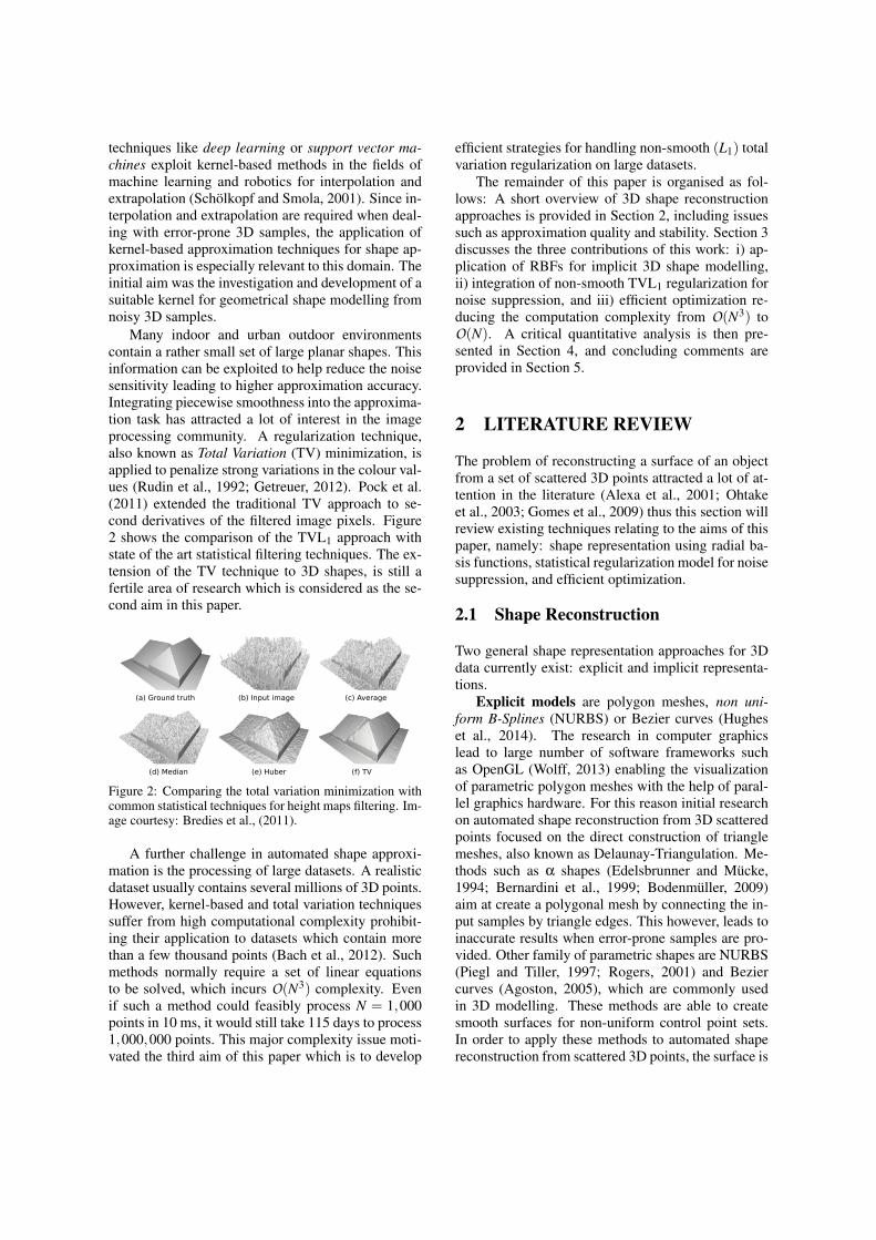
Many indoor and urban outdoor environmentscontain a rather small set of large planar shapes. Thisinformation can be exploited to help reduce the noisesensitivity leading to higher approximation accuracy.Integrating piecewise smoothness into the approxima-tion task has attracted a lot of interest in the imageprocessing community. A regularization technique,also known as Total Variation (TV) minimization, isapplied to penalize strong variations in the colour val-ues (Rudin et al., 1992; Getreuer, 2012). Pock et al.(2011) extended the traditional TV approach to se-cond derivatives of the filtered image pixels. Figure2 shows the comparison of the TVL1 approach withstate of the art statistical filtering techniques. The ex-tension of the TV technique to 3D shapes, is still afertile area of research which is considered as the se-cond aim in this paper.

(a) Ground truth (b) Input image (c) Average

(d) Median (e) Huber (f) TV

Figure 2: Comparing the total variation minimization withcommon statistical techniques for height maps filtering. Im-age courtesy: Bredies et al., (2011).

A further challenge in automated shape approxi-mation is the processing of large datasets. A realisticdataset usually contains several millions of 3D points.However, kernel-based and total variation techniquessuffer from high computational complexity prohibit-ing their application to datasets which contain morethan a few thousand points (Bach et al., 2012). Suchmethods normally require a set of linear equationsto be solved, which incurs O(N3) complexity. Evenif such a method could feasibly process N = 1,000points in 10 ms, it would still take 115 days to process1,000,000 points. This major complexity issue moti-vated the third aim of this paper which is to develop

efficient strategies for handling non-smooth (L1) totalvariation regularization on large datasets.

The remainder of this paper is organised as fol-lows: A short overview of 3D shape reconstructionapproaches is provided in Section 2, including issuessuch as approximation quality and stability. Section 3discusses the three contributions of this work: i) ap-plication of RBFs for implicit 3D shape modelling,ii) integration of non-smooth TVL1 regularization fornoise suppression, and iii) efficient optimization re-ducing the computation complexity from O(N3) toO(N). A critical quantitative analysis is then pre-sented in Section 4, and concluding comments areprovided in Section 5.

2 LITERATURE REVIEW

The problem of reconstructing a surface of an objectfrom a set of scattered 3D points attracted a lot of at-tention in the literature (Alexa et al., 2001; Ohtakeet al., 2003; Gomes et al., 2009) thus this section willreview existing techniques relating to the aims of thispaper, namely: shape representation using radial ba-sis functions, statistical regularization model for noisesuppression, and efficient optimization.

2.1 Shape Reconstruction

Two general shape representation approaches for 3Ddata currently exist: explicit and implicit representa-tions.

Explicit models are polygon meshes, non uni-form B-Splines (NURBS) or Bezier curves (Hugheset al., 2014). The research in computer graphicslead to large number of software frameworks suchas OpenGL (Wolff, 2013) enabling the visualizationof parametric polygon meshes with the help of paral-lel graphics hardware. For this reason initial researchon automated shape reconstruction from 3D scatteredpoints focused on the direct construction of trianglemeshes, also known as Delaunay-Triangulation. Me-thods such as α shapes (Edelsbrunner and Mucke,1994; Bernardini et al., 1999; Bodenmuller, 2009)aim at create a polygonal mesh by connecting the in-put samples by triangle edges. This however, leads toinaccurate results when error-prone samples are pro-vided. Other family of parametric shapes are NURBS(Piegl and Tiller, 1997; Rogers, 2001) and Beziercurves (Agoston, 2005), which are commonly usedin 3D modelling. These methods are able to createsmooth surfaces for non-uniform control point sets.In order to apply these methods to automated shapereconstruction from scattered 3D points, the surface is

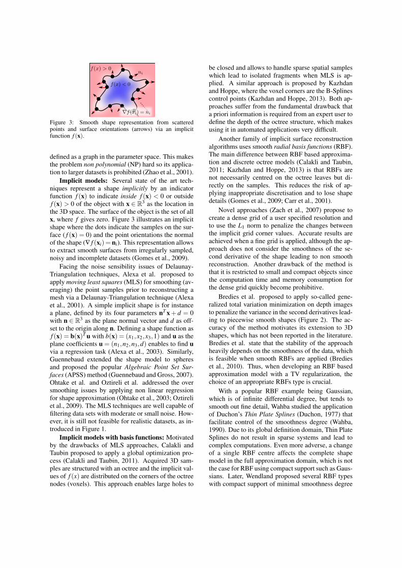
Figure 3: Smooth shape representation from scatteredpoints and surface orientations (arrows) via an implicitfunction f (x).

defined as a graph in the parameter space. This makesthe problem non polynomial (NP) hard so its applica-tion to larger datasets is prohibited (Zhao et al., 2001).

Implicit models: Several state of the art tech-niques represent a shape implicitly by an indicatorfunction f (x) to indicate inside f (x) < 0 or outsidef (x) > 0 of the object with x ∈ R3 as the location inthe 3D space. The surface of the object is the set of allx, where f gives zero. Figure 3 illustrates an implicitshape where the dots indicate the samples on the sur-face ( f (x) = 0) and the point orientations the normalof the shape (∇ f (xi) = ni). This representation allowsto extract smooth surfaces from irregularly sampled,noisy and incomplete datasets (Gomes et al., 2009).

Facing the noise sensibility issues of Delaunay-Triangulation techniques, Alexa et al. proposed toapply moving least squares (MLS) for smoothing (av-eraging) the point samples prior to reconstructing amesh via a Delaunay-Triangulation technique (Alexaet al., 2001). A simple implicit shape is for instancea plane, defined by its four parameters nT x+ d = 0with n ∈ R3 as the plane normal vector and d as off-set to the origin along n. Defining a shape function asf (x) = b(x)T u with b(x) = (x1,x2,x3,1) and u as theplane coefficients u = (n1,n2,n3,d) enables to find uvia a regression task (Alexa et al., 2003). Similarly,Guennebaud extended the shape model to spheresand proposed the popular Algebraic Point Set Sur-faces (APSS) method (Guennebaud and Gross, 2007).Ohtake et al. and Oztireli et al. addressed the oversmoothing issues by applying non linear regressionfor shape approximation (Ohtake et al., 2003; Oztireliet al., 2009). The MLS techniques are well capable offiltering data sets with moderate or small noise. How-ever, it is still not feasible for realistic datasets, as in-troduced in Figure 1.

Implicit models with basis functions: Motivatedby the drawbacks of MLS approaches, Calakli andTaubin proposed to apply a global optimization pro-cess (Calakli and Taubin, 2011). Acquired 3D sam-ples are structured with an octree and the implicit val-ues of f (x) are distributed on the corners of the octreenodes (voxels). This approach enables large holes to

be closed and allows to handle sparse spatial sampleswhich lead to isolated fragments when MLS is ap-plied. A similar approach is proposed by Kazhdanand Hoppe, where the voxel corners are the B-Splinescontrol points (Kazhdan and Hoppe, 2013). Both ap-proaches suffer from the fundamental drawback thata priori information is required from an expert user todefine the depth of the octree structure, which makesusing it in automated applications very difficult.

Another family of implicit surface reconstructionalgorithms uses smooth radial basis functions (RBF).The main difference between RBF based approxima-tion and discrete octree models (Calakli and Taubin,2011; Kazhdan and Hoppe, 2013) is that RBFs arenot necessarily centred on the octree leaves but di-rectly on the samples. This reduces the risk of ap-plying inappropriate discretisation and to lose shapedetails (Gomes et al., 2009; Carr et al., 2001).

Novel approaches (Zach et al., 2007) propose tocreate a dense grid of a user specified resolution andto use the L1 norm to penalize the changes betweenthe implicit grid corner values. Accurate results areachieved when a fine grid is applied, although the ap-proach does not consider the smoothness of the se-cond derivative of the shape leading to non smoothreconstruction. Another drawback of the method isthat it is restricted to small and compact objects sincethe computation time and memory consumption forthe dense grid quickly become prohibitive.

Bredies et al. proposed to apply so-called gene-ralized total variation minimization on depth imagesto penalize the variance in the second derivatives lead-ing to piecewise smooth shapes (Figure 2). The ac-curacy of the method motivates its extension to 3Dshapes, which has not been reported in the literature.Bredies et al. state that the stability of the approachheavily depends on the smoothness of the data, whichis feasible when smooth RBFs are applied (Bredieset al., 2010). Thus, when developing an RBF basedapproximation model with a TV regularization, thechoice of an appropriate RBFs type is crucial.

With a popular RBF example being Gaussian,which is of infinite differential degree, but tends tosmooth out fine detail, Wahba studied the applicationof Duchon’s Thin Plate Splines (Duchon, 1977) thatfacilitate control of the smoothness degree (Wahba,1990). Due to its global definition domain, Thin PlateSplines do not result in sparse systems and lead tocomplex computations. Even more adverse, a changeof a single RBF centre affects the complete shapemodel in the full approximation domain, which is notthe case for RBF using compact support such as Gaus-sians. Later, Wendland proposed several RBF typeswith compact support of minimal smoothness degree

(Wendland, 1995). Wendland’s RBFs also controlthe smoothness of the approximated function and stilllead to sparse and efficient linear regression systems.Moreover, as presented in Section 3, the smaller thesmoothness degree the more stable is the regressionprocess. The Thin Plate RBFs, however, have beenshown to achieve superior approximation quality inthe presence of noise (Tennakoon et al., 2013). Impor-tant aspects when selecting an appropriate RBF typeare presented in Section 3.1.

2.2 Efficient L1 Optimization

Extending the shape approximation with a L1 penaltyrequires more advanced techniques to solve the opti-mization task. This issue has been discussed for sometime in the statistics and numerical optimization com-munity. However, efficient techniques being capableof dealing with thousands or millions of data samplesare in the current research focus.

Tibshirani proposed the Least Absolute Shrink-age and Selection (Lasso) technique to minimize costfunctions such as

‖ y−Kα ‖22 + ‖ α ‖1 (1)

with ‖ α ‖1= ∑Nj |αi| enabling its application on

images with several hundreds of thousands entries inα (Tibshirani, 1994). This form is common for regres-sion problems, where the signal y is approximated lin-early by the model matrix K. The additional ‖ · ‖1penalty term enforces only a small amount of non ze-ros entries in α. This behaviour is suitable for prob-lems where the vector α is expected to have many zeroentries. A common application is for example signalapproximation by only a small set of frequencies rep-resented by α.When representing a shape with N RBFs

f (x) =N

∑i

ϕ(x,xi)αi = kTα (2)

with ki = ϕ(x,xi) its second derivatives are penalizedby ‖Dα ‖1 with D j,i = ∂2

xxϕ(x j,xi). This way ‖Dα ‖1penalizes the amount of non smooth regions in theextracted model. However, since the entries in Dα

are not separated as it is the case in (1), such prob-lems are more difficult to solve and using the Lassotechnique is not possible. Initially, interior active setsmethods have been applied to solve the TVL1 objec-tive (Alizadeh et al., 2003). Chen et al. additionallydemonstrated that the efficiency of primal-dual me-thods is of magnitudes higher than of the interior me-thods (Chen et al., 2010). Also Goldstein et al. pro-posed a primal-dual approach known as the BregmanSplit (Bregman, 1967) to separate the smooth data

term fd =‖ y−Kα ‖22 from the non smooth regulariza-

tion term fr =‖ Dα ‖1 and to optimize each of themindependently (Goldstein and Osher, 2009). Boyd etal. extended the Bregman Split approach by Dykstra’salternating projections technique (Dykstra, 1982) andproposed the Alternating Direction Method of Mul-tipliers (ADMM) (Boyd et al., 2011), which furtherimproves the convergence. Discussions related to ap-plications of ADMM are reported by Parikh and Boyd(2014).

The bottleneck of ADMM is the minimizationof the smooth part fd =‖ y−Kα ‖2

2. Solving thisfor α with efficient Cholesky factorization suffersfrom a complexity of O(N3). However, an iterativelinear solver such as Jacobian or Gauss-Seidel mayreduce the complexity to O(N) as discussed by Saador Friedman et al. relating to L1 regularization (Saad,2003; Friedman et al., 2010). Nevertheless, furtherinvestigations on the applicability of iterative linearsolvers and ADMM on 3D shape modelling do notexist.

2.3 Summary

The presented state of the art in robust shape approxi-mation and optimization methods covers several ap-propriate options for investigation. Table 1 showsthe seminal methods summarizing the benefits anddrawbacks of each technique. The TVL1 approach(Bredies et al., 2010) delivers high quality with arte-facts such as missing data, noise, outliers, or sharpedges in the image domain. This technique, how-ever, suffers from high computational complexity andneeds to be extended to 3D shape approximation.Section 2.2 states that the ADMM technique is ex-pected to outperform the efficiency of existing TVL1algorithms when extended with an iterative solver.

The next Section investigates the impact of dif-ferent RBFs applied for signal and shape approxima-tion from scattered 3D points before the new ADMMtechnique for TVL1 optimization on large datasets ispresented.

3 THE METHOD

The first part of this section pursues the first researchobjective and discusses the fundamentals of RBFbased approximation and compares different types ofRBFs with respect to quality and stability when leastsquares optimization is performed. Section 3.2 ap-plies the proposed RBFs and defines the convex opti-mization task to perform shape reconstruction from

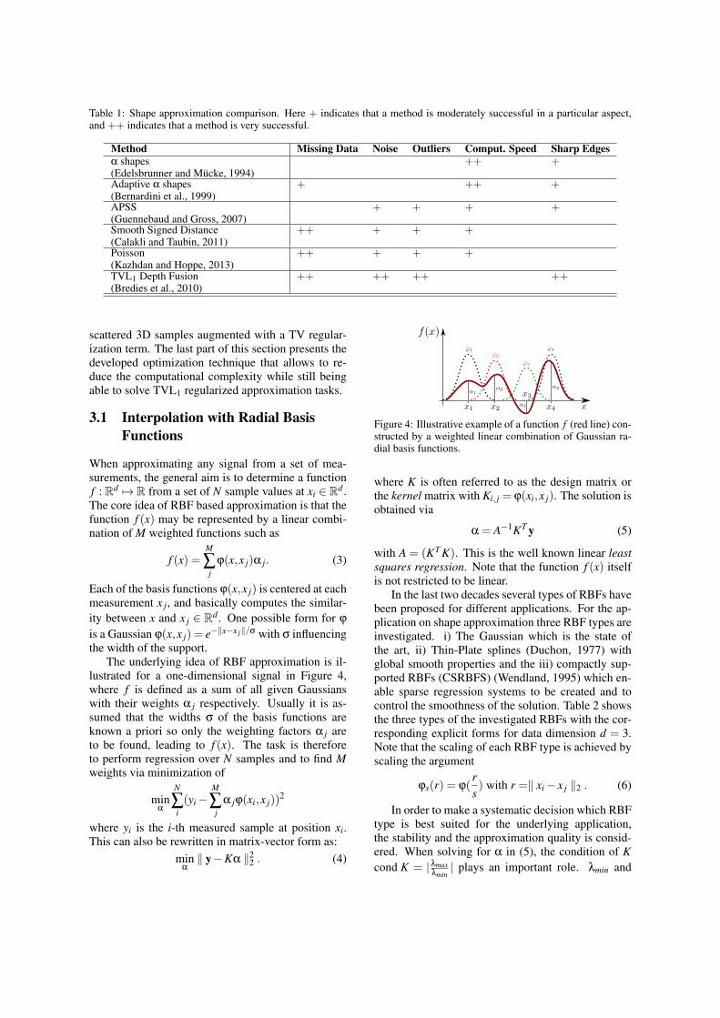
Table 1: Shape approximation comparison. Here + indicates that a method is moderately successful in a particular aspect,and ++ indicates that a method is very successful.

Method Missing Data Noise Outliers Comput. Speed Sharp Edgesα shapes(Edelsbrunner and Mucke, 1994)

++ +

Adaptive α shapes(Bernardini et al., 1999)

+ ++ +

APSS(Guennebaud and Gross, 2007)

+ + + +

Smooth Signed Distance(Calakli and Taubin, 2011)

++ + + +

Poisson(Kazhdan and Hoppe, 2013)

++ + + +

TVL1 Depth Fusion(Bredies et al., 2010)

++ ++ ++ ++

scattered 3D samples augmented with a TV regular-ization term. The last part of this section presents thedeveloped optimization technique that allows to re-duce the computational complexity while still beingable to solve TVL1 regularized approximation tasks.

3.1 Interpolation with Radial BasisFunctions

When approximating any signal from a set of mea-surements, the general aim is to determine a functionf : Rd 7→ R from a set of N sample values at xi ∈ Rd .The core idea of RBF based approximation is that thefunction f (x) may be represented by a linear combi-nation of M weighted functions such as

f (x) =M

∑j

ϕ(x,x j)α j. (3)

Each of the basis functions ϕ(x,x j) is centered at eachmeasurement x j, and basically computes the similar-ity between x and x j ∈ Rd . One possible form for ϕ

is a Gaussian ϕ(x,x j) = e−‖x−x j‖/σ with σ influencingthe width of the support.

The underlying idea of RBF approximation is il-lustrated for a one-dimensional signal in Figure 4,where f is defined as a sum of all given Gaussianswith their weights α j respectively. Usually it is as-sumed that the widths σ of the basis functions areknown a priori so only the weighting factors α j areto be found, leading to f (x). The task is thereforeto perform regression over N samples and to find Mweights via minimization of

minα

N

∑i(yi−

M

∑j

α jϕ(xi,x j))2

where yi is the i-th measured sample at position xi.This can also be rewritten in matrix-vector form as:

minα‖ y−Kα ‖2

2 . (4)

Figure 4: Illustrative example of a function f (red line) con-structed by a weighted linear combination of Gaussian ra-dial basis functions.

where K is often referred to as the design matrix orthe kernel matrix with Ki, j = ϕ(xi,x j). The solution isobtained via

α = A−1KT y (5)

with A = (KT K). This is the well known linear leastsquares regression. Note that the function f (x) itselfis not restricted to be linear.

In the last two decades several types of RBFs havebeen proposed for different applications. For the ap-plication on shape approximation three RBF types areinvestigated. i) The Gaussian which is the state ofthe art, ii) Thin-Plate splines (Duchon, 1977) withglobal smooth properties and the iii) compactly sup-ported RBFs (CSRBFS) (Wendland, 1995) which en-able sparse regression systems to be created and tocontrol the smoothness of the solution. Table 2 showsthe three types of the investigated RBFs with the cor-responding explicit forms for data dimension d = 3.Note that the scaling of each RBF type is achieved byscaling the argument

ϕs(r) = ϕ(rs) with r =‖ xi− x j ‖2 . (6)

In order to make a systematic decision which RBFtype is best suited for the underlying application,the stability and the approximation quality is consid-ered. When solving for α in (5), the condition of Kcond K = |λmax

λmin| plays an important role. λmin and

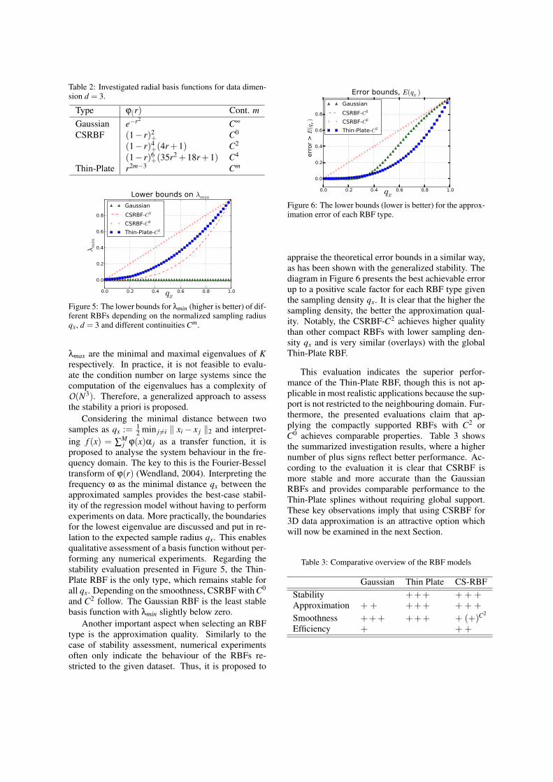
Table 2: Investigated radial basis functions for data dimen-sion d = 3.

Type ϕ(r) Cont. mGaussian e−r2

C∞

CSRBF (1− r)2+ C0

(1− r)4+(4r+1) C2

(1− r)6+(35r2 +18r+1) C4

Thin-Plate r2m−3 Cm

Figure 5: The lower bounds for λmin (higher is better) of dif-ferent RBFs depending on the normalized sampling radiusqx, d = 3 and different continuities Cm.

λmax are the minimal and maximal eigenvalues of Krespectively. In practice, it is not feasible to evalu-ate the condition number on large systems since thecomputation of the eigenvalues has a complexity ofO(N3). Therefore, a generalized approach to assessthe stability a priori is proposed.

Considering the minimal distance between twosamples as qx := 1

2 min j 6=i ‖ xi− x j ‖2 and interpret-ing f (x) = ∑

Mj ϕ(x)α j as a transfer function, it is

proposed to analyse the system behaviour in the fre-quency domain. The key to this is the Fourier-Besseltransform of ϕ(r) (Wendland, 2004). Interpreting thefrequency ω as the minimal distance qx between theapproximated samples provides the best-case stabil-ity of the regression model without having to performexperiments on data. More practically, the boundariesfor the lowest eigenvalue are discussed and put in re-lation to the expected sample radius qx. This enablesqualitative assessment of a basis function without per-forming any numerical experiments. Regarding thestability evaluation presented in Figure 5, the Thin-Plate RBF is the only type, which remains stable forall qx. Depending on the smoothness, CSRBF with C0

and C2 follow. The Gaussian RBF is the least stablebasis function with λmin slightly below zero.

Another important aspect when selecting an RBFtype is the approximation quality. Similarly to thecase of stability assessment, numerical experimentsoften only indicate the behaviour of the RBFs re-stricted to the given dataset. Thus, it is proposed to

Figure 6: The lower bounds (lower is better) for the approx-imation error of each RBF type.

appraise the theoretical error bounds in a similar way,as has been shown with the generalized stability. Thediagram in Figure 6 presents the best achievable errorup to a positive scale factor for each RBF type giventhe sampling density qx. It is clear that the higher thesampling density, the better the approximation qual-ity. Notably, the CSRBF-C2 achieves higher qualitythan other compact RBFs with lower sampling den-sity qx and is very similar (overlays) with the globalThin-Plate RBF.

This evaluation indicates the superior perfor-mance of the Thin-Plate RBF, though this is not ap-plicable in most realistic applications because the sup-port is not restricted to the neighbouring domain. Fur-thermore, the presented evaluations claim that ap-plying the compactly supported RBFs with C2 orC0 achieves comparable properties. Table 3 showsthe summarized investigation results, where a highernumber of plus signs reflect better performance. Ac-cording to the evaluation it is clear that CSRBF ismore stable and more accurate than the GaussianRBFs and provides comparable performance to theThin-Plate splines without requiring global support.These key observations imply that using CSRBF for3D data approximation is an attractive option whichwill now be examined in the next Section.

Table 3: Comparative overview of the RBF models

Gaussian Thin Plate CS-RBFStability +++ + + +Approximation + + +++ + + +

Smoothness +++ +++ + (+)C2

Efficiency + + +

3.2 Shape Reconstruction fromScattered Points

The principal idea of shape modelling with RBF isto extract an implicit function which represents theshape by its zero value as introduced in Figure 3.More formally, an algebraic function f (x), f :R3 7→Rneeds to be constructed by regression. Given a set ofmeasured 3D points, the task is further to find a func-tion f (x) which returns zero on every i-th sample xiand interpolates well between the samples. Since thezero level alone does not provide information aboutthe orientation of the surface, the surface normals niat every sample are used as constraints for the gradi-ent ∇ f (x) wrt. x. The task is now to find f (xi) = 0giving zero at every sample position and ∇ f (xi) = ni.Integrating all this information, a convex cost func-tional is defined.

minα

N

∑i‖ f (xi) ‖2

2 + ‖ ni−∇ f (xi) ‖22 (7)

To simplify the optimization problem the normaliza-tion term ‖∇ f (xi) ‖2= 1 is omitted. In order to obtainthe gradient ∇ f , only the gradient of ϕ needs to becomputed, which is precomputed analytically. Putting(7) into matrix notation leads to the short form of thecost function

minααα‖ Kααα ‖2

2 + ‖ n−K∇α ‖22 . (8)

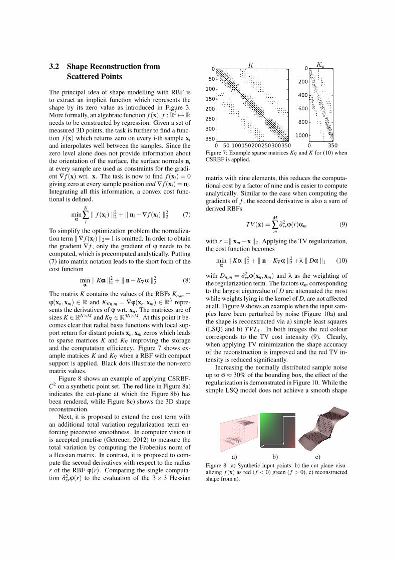
The matrix K contains the values of the RBFs Kn,m =

ϕ(xn,xm) ∈ R and K∇n,m = ∇ϕ(xn,xm) ∈ R3 repre-sents the derivatives of ϕ wrt. xn. The matrices are ofsizes K ∈RN×M and K∇ ∈R3N×M . At this point it be-comes clear that radial basis functions with local sup-port return for distant points xn,xm zeros which leadsto sparse matrices K and K∇ improving the storageand the computation efficiency. Figure 7 shows ex-ample matrices K and K∇ when a RBF with compactsupport is applied. Black dots illustrate the non-zeromatrix values.

Figure 8 shows an example of applying CSRBF-C2 on a synthetic point set. The red line in Figure 8a)indicates the cut-plane at which the Figure 8b) hasbeen rendered, while Figure 8c) shows the 3D shapereconstruction.

Next, it is proposed to extend the cost term withan additional total variation regularization term en-forcing piecewise smoothness. In computer vision itis accepted practise (Getreuer, 2012) to measure thetotal variation by computing the Frobenius norm ofa Hessian matrix. In contrast, it is proposed to com-pute the second derivatives with respect to the radiusr of the RBF ϕ(r). Comparing the single computa-tion ∂2

rrϕ(r) to the evaluation of the 3× 3 Hessian

Figure 7: Example sparse matrices K∇ and K for (10) whenCSRBF is applied.

matrix with nine elements, this reduces the computa-tional cost by a factor of nine and is easier to computeanalytically. Similar to the case when computing thegradients of f , the second derivative is also a sum ofderived RBFs

TV (x) =M

∑m

∂2rrϕ(r)αm (9)

with r =‖ xm−x ‖2. Applying the TV regularization,the cost function becomes

minα‖ Kα ‖2

2 + ‖ n−K∇α ‖22 +λ ‖ Dα ‖1 (10)

with Dn,m = ∂2rrϕ(xn,xm) and λ as the weighting of

the regularization term. The factors αm correspondingto the largest eigenvalue of D are attenuated the mostwhile weights lying in the kernel of D, are not affectedat all. Figure 9 shows an example when the input sam-ples have been perturbed by noise (Figure 10a) andthe shape is reconstructed via a) simple least squares(LSQ) and b) TV L1. In both images the red colourcorresponds to the TV cost intensity (9). Clearly,when applying TV minimization the shape accuracyof the reconstruction is improved and the red TV in-tensity is reduced significantly.

Increasing the normally distributed sample noiseup to σ ≈ 30% of the bounding box, the effect of theregularization is demonstrated in Figure 10. While thesimple LSQ model does not achieve a smooth shape

a) b) c)Figure 8: a) Synthetic input points, b) the cut plane visu-alizing f (x) as red ( f < 0) green ( f > 0), c) reconstructedshape from a).

(Figure 10b) the new regularized approach in Figure10c) shows considerable perceptual improvement interms of the quality of the shape reconstruction.

In the next section, the proposed numerical tech-nique to efficiently solve the TVL1 task is presented.

a) b)Figure 9: a) The TV cost (red) overlaid with the unregular-ized shape obtained via LSQ. b) The reduced TV cost (lessred colour) after performing regularized approximation fol-lowing (10).

3.3 TVL1 Solver

To minimize the task (10) it is proposed to apply theLagrangian approach from the Alternating DirectionMethod of Multipliers (ADMM) (Boyd et al., 2011).Formally, (10) is restated to

minα,z

L(α,z) = f1(α)+ f2(z)+

bT (Dα− z)+ρ

2‖ Dα− z ‖2

2

(11)

where f1(α) is the data part from (10) depending onα, and f2(z) = λ ‖ z ‖1 is the non-smooth regular-ization part weighted by λ. The basic approach isto minimize for α, then for z iteratively. The termsbT (Dα− z) and ‖ Dα− z ‖2 make sure that Dα isclose to z after an iteration finishes reducing the du-ality gap. This restriction is controlled by ρ which isusually a large scalar. The iterative optimization pro-cess between α and z is summarized in Algorithm 1.The minimization for z involves a sub gradient over‖ · ‖1 and its solution is known as the shrinkage oper-ator (Efron et al., 2004) being applied on each elementzi independently:

zi = shrink(a,b)= a−b · sign(b−a)+

where a =bi

ρ+(Dα)i, b =

λ

ρ

(12)

with (Dα)i as the i-th element of the vector Dα andsign(b−a)+ gives 1 if b > a and zero otherwise.

Algorithm 1: ADMM for L1 approximation1. Solve for α:

(KT∇

K∇ +KT K +ρDT D)α = KT∇

n+DT (ρz−b).

2. Evaluate: zk+1i = shrink( bi

ρ+(Dα)i,λ/ρ)

3. Evaluate: bk+1 := bk +(Dαk+1− zk+1)ρ

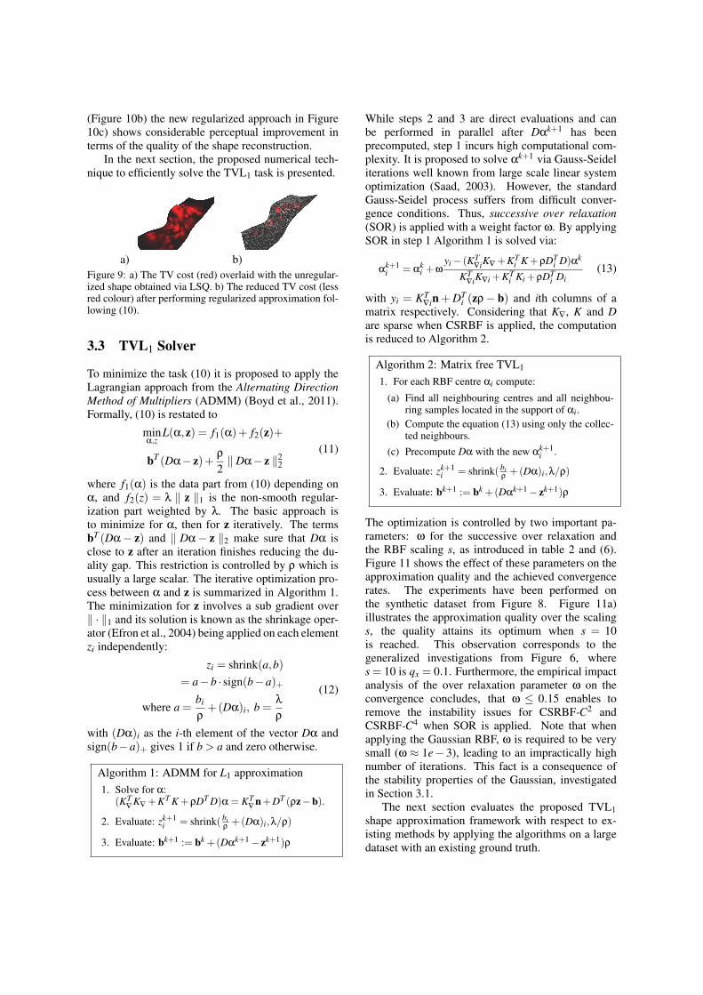
While steps 2 and 3 are direct evaluations and canbe performed in parallel after Dαk+1 has beenprecomputed, step 1 incurs high computational com-plexity. It is proposed to solve αk+1 via Gauss-Seideliterations well known from large scale linear systemoptimization (Saad, 2003). However, the standardGauss-Seidel process suffers from difficult conver-gence conditions. Thus, successive over relaxation(SOR) is applied with a weight factor ω. By applyingSOR in step 1 Algorithm 1 is solved via:

αk+1i = α

ki +ω

yi− (KT∇iK∇ +KT

i K +ρDTi D)αk

KT∇iK∇i +KT

i Ki +ρDTi Di

(13)

with yi = KT∇in + DT

i (zρ− b) and ith columns of amatrix respectively. Considering that K∇, K and Dare sparse when CSRBF is applied, the computationis reduced to Algorithm 2.

Algorithm 2: Matrix free TVL1

1. For each RBF centre αi compute:

(a) Find all neighbouring centres and all neighbou-ring samples located in the support of αi.

(b) Compute the equation (13) using only the collec-ted neighbours.

(c) Precompute Dα with the new αk+1i .

2. Evaluate: zk+1i = shrink( bi

ρ+(Dα)i,λ/ρ)

3. Evaluate: bk+1 := bk +(Dαk+1− zk+1)ρ

The optimization is controlled by two important pa-rameters: ω for the successive over relaxation andthe RBF scaling s, as introduced in table 2 and (6).Figure 11 shows the effect of these parameters on theapproximation quality and the achieved convergencerates. The experiments have been performed onthe synthetic dataset from Figure 8. Figure 11a)illustrates the approximation quality over the scalings, the quality attains its optimum when s = 10is reached. This observation corresponds to thegeneralized investigations from Figure 6, wheres = 10 is qx = 0.1. Furthermore, the empirical impactanalysis of the over relaxation parameter ω on theconvergence concludes, that ω ≤ 0.15 enables toremove the instability issues for CSRBF-C2 andCSRBF-C4 when SOR is applied. Note that whenapplying the Gaussian RBF, ω is required to be verysmall (ω ≈ 1e− 3), leading to an impractically highnumber of iterations. This fact is a consequence ofthe stability properties of the Gaussian, investigatedin Section 3.1.

The next section evaluates the proposed TVL1shape approximation framework with respect to ex-isting methods by applying the algorithms on a largedataset with an existing ground truth.

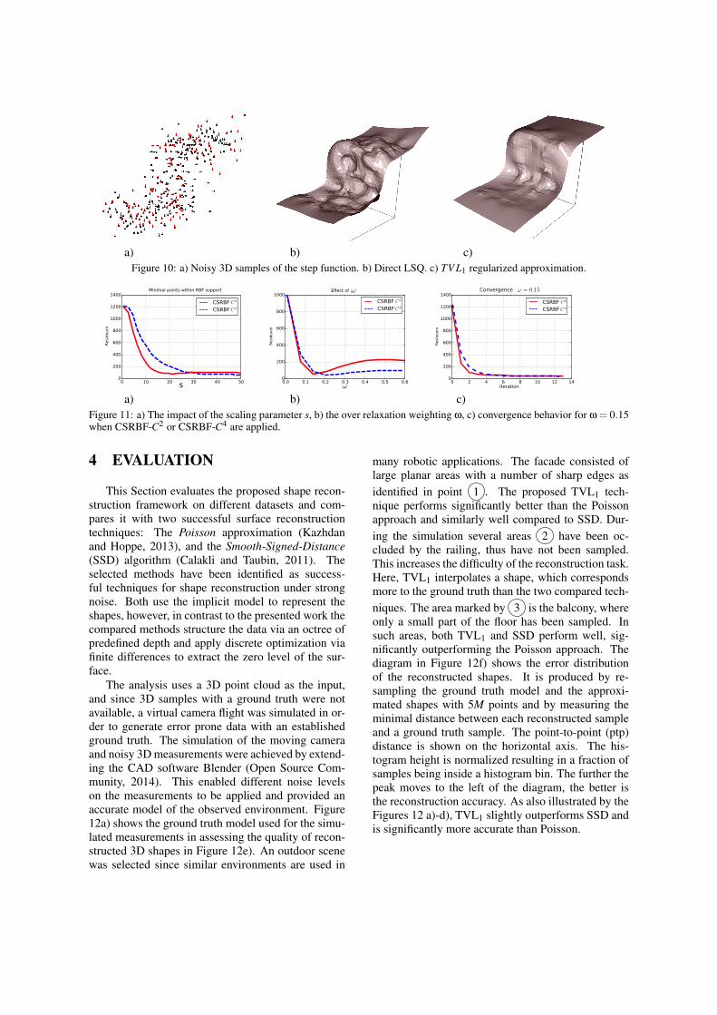
a) b) c)Figure 10: a) Noisy 3D samples of the step function. b) Direct LSQ. c) TV L1 regularized approximation.

Minimal points within RBF support

Resi

duum

s

Resi

duum

Effect of

Iteration

Resi

duum

Convergence

a) b) c)Figure 11: a) The impact of the scaling parameter s, b) the over relaxation weighting ω, c) convergence behavior for ω = 0.15when CSRBF-C2 or CSRBF-C4 are applied.

4 EVALUATION

This Section evaluates the proposed shape recon-struction framework on different datasets and com-pares it with two successful surface reconstructiontechniques: The Poisson approximation (Kazhdanand Hoppe, 2013), and the Smooth-Signed-Distance(SSD) algorithm (Calakli and Taubin, 2011). Theselected methods have been identified as success-ful techniques for shape reconstruction under strongnoise. Both use the implicit model to represent theshapes, however, in contrast to the presented work thecompared methods structure the data via an octree ofpredefined depth and apply discrete optimization viafinite differences to extract the zero level of the sur-face.

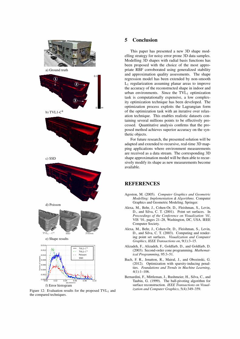
The analysis uses a 3D point cloud as the input,and since 3D samples with a ground truth were notavailable, a virtual camera flight was simulated in or-der to generate error prone data with an establishedground truth. The simulation of the moving cameraand noisy 3D measurements were achieved by extend-ing the CAD software Blender (Open Source Com-munity, 2014). This enabled different noise levelson the measurements to be applied and provided anaccurate model of the observed environment. Figure12a) shows the ground truth model used for the simu-lated measurements in assessing the quality of recon-structed 3D shapes in Figure 12e). An outdoor scenewas selected since similar environments are used in

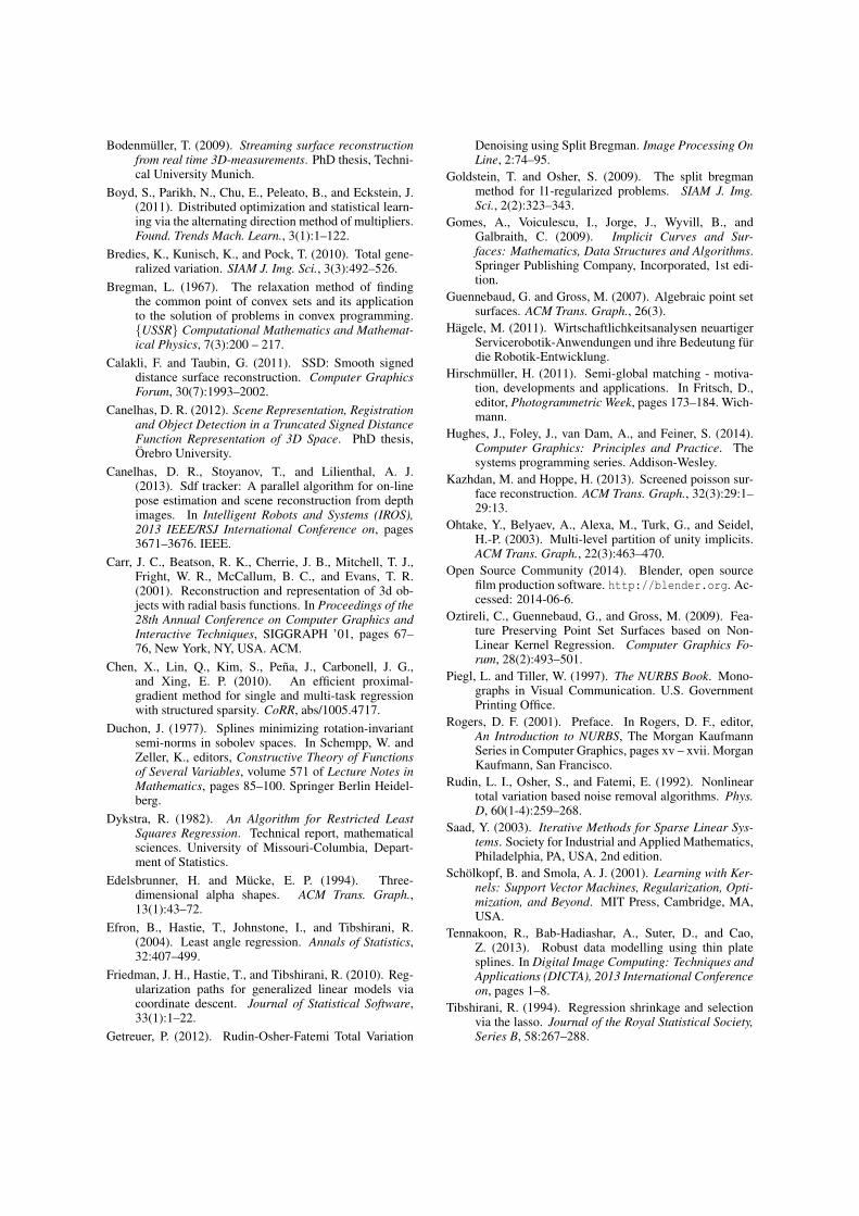
many robotic applications. The facade consisted oflarge planar areas with a number of sharp edges asidentified in point 1 . The proposed TVL1 tech-nique performs significantly better than the Poissonapproach and similarly well compared to SSD. Dur-ing the simulation several areas 2 have been oc-cluded by the railing, thus have not been sampled.This increases the difficulty of the reconstruction task.Here, TVL1 interpolates a shape, which correspondsmore to the ground truth than the two compared tech-niques. The area marked by 3 is the balcony, whereonly a small part of the floor has been sampled. Insuch areas, both TVL1 and SSD perform well, sig-nificantly outperforming the Poisson approach. Thediagram in Figure 12f) shows the error distributionof the reconstructed shapes. It is produced by re-sampling the ground truth model and the approxi-mated shapes with 5M points and by measuring theminimal distance between each reconstructed sampleand a ground truth sample. The point-to-point (ptp)distance is shown on the horizontal axis. The his-togram height is normalized resulting in a fraction ofsamples being inside a histogram bin. The further thepeak moves to the left of the diagram, the better isthe reconstruction accuracy. As also illustrated by theFigures 12 a)-d), TVL1 slightly outperforms SSD andis significantly more accurate than Poisson.

a) Ground truth

1

2

3

0.1

0 m

b) TVL1-C4

c) SSD

d) Poisson

e) Shape results

ptp-distance

fract

ion o

f sa

mple

s

TVL1-

TVL1-

Poisson

SSD

f) Error histogramFigure 12: Evaluation results for the proposed TVL1 andthe compared techniques.

5 Conclusion

This paper has presented a new 3D shape mod-elling strategy for noisy error prone 3D data samples.Modelling 3D shapes with radial basis functions hasbeen proposed with the choice of the most appro-priate RBF corroborated using generalized stabilityand approximation quality assessments. The shaperegression model has been extended by non-smoothL1 regularization assuming planar areas to improvethe accuracy of the reconstructed shape in indoor andurban environments. Since the TVL1 optimizationtask is computationally expensive, a low complex-ity optimization technique has been developed. Theoptimization process exploits the Lagrangian formof the optimization task with an iterative over relax-ation technique. This enables realistic datasets con-taining several millions points to be effectively pro-cessed. Quantitative analysis confirms that the pro-posed method achieves superior accuracy on the syn-thetic objects.

For future research, the presented solution will beadapted and extended to recursive, real-time 3D map-ping applications where environment measurementsare received as a data stream. The corresponding 3Dshape approximation model will be then able to recur-sively modify its shape as new measurements becomeavailable.

REFERENCES

Agoston, M. (2005). Computer Graphics and GeometricModelling: Implementation & Algorithms. ComputerGraphics and Geometric Modeling. Springer.

Alexa, M., Behr, J., Cohen-Or, D., Fleishman, S., Levin,D., and Silva, C. T. (2001). Point set surfaces. InProceedings of the Conference on Visualization ’01,VIS ’01, pages 21–28, Washington, DC, USA. IEEEComputer Society.

Alexa, M., Behr, J., Cohen-Or, D., Fleishman, S., Levin,D., and Silva, C. T. (2003). Computing and render-ing point set surfaces. Visualization and ComputerGraphics, IEEE Transactions on, 9(1):3–15.

Alizadeh, F., Alizadeh, F., Goldfarb, D., and Goldfarb, D.(2003). Second-order cone programming. Mathemat-ical Programming, 95:3–51.

Bach, F. R., Jenatton, R., Mairal, J., and Obozinski, G.(2012). Optimization with sparsity-inducing penal-ties. Foundations and Trends in Machine Learning,4(1):1–106.

Bernardini, F., Mittleman, J., Rushmeier, H., Silva, C., andTaubin, G. (1999). The ball-pivoting algorithm forsurface reconstruction. IEEE Transactions on Visual-ization and Computer Graphics, 5(4):349–359.

Bodenmuller, T. (2009). Streaming surface reconstructionfrom real time 3D-measurements. PhD thesis, Techni-cal University Munich.

Boyd, S., Parikh, N., Chu, E., Peleato, B., and Eckstein, J.(2011). Distributed optimization and statistical learn-ing via the alternating direction method of multipliers.Found. Trends Mach. Learn., 3(1):1–122.

Bredies, K., Kunisch, K., and Pock, T. (2010). Total gene-ralized variation. SIAM J. Img. Sci., 3(3):492–526.

Bregman, L. (1967). The relaxation method of findingthe common point of convex sets and its applicationto the solution of problems in convex programming.{USSR} Computational Mathematics and Mathemat-ical Physics, 7(3):200 – 217.

Calakli, F. and Taubin, G. (2011). SSD: Smooth signeddistance surface reconstruction. Computer GraphicsForum, 30(7):1993–2002.

Canelhas, D. R. (2012). Scene Representation, Registrationand Object Detection in a Truncated Signed DistanceFunction Representation of 3D Space. PhD thesis,Orebro University.

Canelhas, D. R., Stoyanov, T., and Lilienthal, A. J.(2013). Sdf tracker: A parallel algorithm for on-linepose estimation and scene reconstruction from depthimages. In Intelligent Robots and Systems (IROS),2013 IEEE/RSJ International Conference on, pages3671–3676. IEEE.

Carr, J. C., Beatson, R. K., Cherrie, J. B., Mitchell, T. J.,Fright, W. R., McCallum, B. C., and Evans, T. R.(2001). Reconstruction and representation of 3d ob-jects with radial basis functions. In Proceedings of the28th Annual Conference on Computer Graphics andInteractive Techniques, SIGGRAPH ’01, pages 67–76, New York, NY, USA. ACM.

Chen, X., Lin, Q., Kim, S., Pena, J., Carbonell, J. G.,and Xing, E. P. (2010). An efficient proximal-gradient method for single and multi-task regressionwith structured sparsity. CoRR, abs/1005.4717.

Duchon, J. (1977). Splines minimizing rotation-invariantsemi-norms in sobolev spaces. In Schempp, W. andZeller, K., editors, Constructive Theory of Functionsof Several Variables, volume 571 of Lecture Notes inMathematics, pages 85–100. Springer Berlin Heidel-berg.

Dykstra, R. (1982). An Algorithm for Restricted LeastSquares Regression. Technical report, mathematicalsciences. University of Missouri-Columbia, Depart-ment of Statistics.

Edelsbrunner, H. and Mucke, E. P. (1994). Three-dimensional alpha shapes. ACM Trans. Graph.,13(1):43–72.

Efron, B., Hastie, T., Johnstone, I., and Tibshirani, R.(2004). Least angle regression. Annals of Statistics,32:407–499.

Friedman, J. H., Hastie, T., and Tibshirani, R. (2010). Reg-ularization paths for generalized linear models viacoordinate descent. Journal of Statistical Software,33(1):1–22.

Getreuer, P. (2012). Rudin-Osher-Fatemi Total Variation

Denoising using Split Bregman. Image Processing OnLine, 2:74–95.

Goldstein, T. and Osher, S. (2009). The split bregmanmethod for l1-regularized problems. SIAM J. Img.Sci., 2(2):323–343.

Gomes, A., Voiculescu, I., Jorge, J., Wyvill, B., andGalbraith, C. (2009). Implicit Curves and Sur-faces: Mathematics, Data Structures and Algorithms.Springer Publishing Company, Incorporated, 1st edi-tion.

Guennebaud, G. and Gross, M. (2007). Algebraic point setsurfaces. ACM Trans. Graph., 26(3).

Hagele, M. (2011). Wirtschaftlichkeitsanalysen neuartigerServicerobotik-Anwendungen und ihre Bedeutung furdie Robotik-Entwicklung.

Hirschmuller, H. (2011). Semi-global matching - motiva-tion, developments and applications. In Fritsch, D.,editor, Photogrammetric Week, pages 173–184. Wich-mann.

Hughes, J., Foley, J., van Dam, A., and Feiner, S. (2014).Computer Graphics: Principles and Practice. Thesystems programming series. Addison-Wesley.

Kazhdan, M. and Hoppe, H. (2013). Screened poisson sur-face reconstruction. ACM Trans. Graph., 32(3):29:1–29:13.

Ohtake, Y., Belyaev, A., Alexa, M., Turk, G., and Seidel,H.-P. (2003). Multi-level partition of unity implicits.ACM Trans. Graph., 22(3):463–470.

Open Source Community (2014). Blender, open sourcefilm production software. http://blender.org. Ac-cessed: 2014-06-6.

Oztireli, C., Guennebaud, G., and Gross, M. (2009). Fea-ture Preserving Point Set Surfaces based on Non-Linear Kernel Regression. Computer Graphics Fo-rum, 28(2):493–501.

Piegl, L. and Tiller, W. (1997). The NURBS Book. Mono-graphs in Visual Communication. U.S. GovernmentPrinting Office.

Rogers, D. F. (2001). Preface. In Rogers, D. F., editor,An Introduction to NURBS, The Morgan KaufmannSeries in Computer Graphics, pages xv – xvii. MorganKaufmann, San Francisco.

Rudin, L. I., Osher, S., and Fatemi, E. (1992). Nonlineartotal variation based noise removal algorithms. Phys.D, 60(1-4):259–268.

Saad, Y. (2003). Iterative Methods for Sparse Linear Sys-tems. Society for Industrial and Applied Mathematics,Philadelphia, PA, USA, 2nd edition.

Scholkopf, B. and Smola, A. J. (2001). Learning with Ker-nels: Support Vector Machines, Regularization, Opti-mization, and Beyond. MIT Press, Cambridge, MA,USA.

Tennakoon, R., Bab-Hadiashar, A., Suter, D., and Cao,Z. (2013). Robust data modelling using thin platesplines. In Digital Image Computing: Techniques andApplications (DICTA), 2013 International Conferenceon, pages 1–8.

Tibshirani, R. (1994). Regression shrinkage and selectionvia the lasso. Journal of the Royal Statistical Society,Series B, 58:267–288.

Wahba, G. (1990). Spline models for observational data,volume 59 of CBMS-NSF Regional Conference Seriesin Applied Mathematics. Society for Industrial andApplied Mathematics (SIAM), Philadelphia, PA.

Wendland, H. (1995). Piecewise polynomial, positive defi-nite and compactly supported radial functions of mini-mal degree. Advances in Computational Mathematics,4(1):389–396.

Wendland, H. (2004). Scattered Data Approximation. Cam-bridge University Press.

Wolff, D. (2013). OpenGL 4 Shading Language Cookbook,Second Edition. EBL-Schweitzer. Packt Publishing.

Zach, C., Pock, T., and Bischof, H. (2007). A globally opti-mal algorithm for robust tv-l1 range image integration.In Computer Vision, 2007. ICCV 2007. IEEE 11th In-ternational Conference on, pages 1–8.

Zhao, H., Oshery, S., and Fedkiwz, R. (2001). Fast surfacereconstruction using the level set method. In In VLSM01: Proceedings of the IEEE Workshop on Variationaland Level Set Methods.