“R” Programming Language Tutorial

ECE 313 – Section B

University of Illinois at Urbana - Champaign

Outline

• Why R, and R Paradigm • References, Tutorials and links • R Overview • R Interface • R Workspace • Help • R Packages • Input/Output • Reusing Results

Why R?

• It's free! • It runs on a variety of platforms including Windows, Unix and

MacOS. • It provides an unparalleled platform for programming new

statistical methods in an easy and straightforward manner. • It contains advanced statistical routines not yet available in

other packages. • It has state-of-the-art graphics capabilities.

Installing R

• How to download R: – http://www.r-project.org/ – Google: “R” – Windows, Linux, Mac OS X, source – On mindhive:

• user@ba1:~$> R [terminal only] • user@ba1:~$> R –g Tk & [application window]

• Files for this tutorial: – http://web.mit.edu/tkp/www/R/R_Tutorial_Data.txt – http://web.mit.edu/tkp/www/R/R_Tutorial_Inputs.txt

Tutorials

• Each of the following tutorials are in PDF format. • P. Kuhnert & B. Venables, An Introduction to R: Software for

Statistical Modeling & Computing • J.H. Maindonald, Using R for Data Analysis and Graphics • B. Muenchen, R for SAS and SPSS Users • W.J. Owen, The R Guide • D. Rossiter, Introduction to the R Project for Statistical Computing

for Use at the ITC • W.N. Venebles & D. M. Smith, An Introduction to R

Where to find R help and resources on the web

• R wiki: http://rwiki.sciviews.org/doku.php

• R graph gallery: http://addictedtor.free.fr/graphiques/thumbs.php

• Kickstarting R: http://cran.r-project.org/doc/contrib/Lemon-kickstart/

ISBN

: 978

0596

8017

00

More Links

• R time series tutorial • R Concepts and Data Types presentation by Deepayan Sarkar • Interpreting Output From lm() • The R Wiki • An Introduction to R • Import / Export Manual • R Reference Cards

Introduction • R is “GNU S” — A language and environment for data

manipula-tion, calculation and graphical display. – R is similar to the award-winning S system, which was developed at Bell

Laboratories by John Chambers et al. – a suite of operators for calculations on arrays, in particular matrices, – a large, coherent, integrated collection of intermediate tools for interactive

data analysis, – graphical facilities for data analysis and display either directly at the computer

or on hardcopy – a well developed programming language which includes conditionals, loops,

user defined recursive functions and input and output facilities.

Introduction

• The core of R is an interpreted computer language. – It allows branching and looping as well as modular programming using functions. – Most of the user-visible functions in R are written in R, calling upon a smaller set

of internal primitives. – It is possible for the user to interface to procedures written in C, C++ or

FORTRAN languages for efficiency, and also to write additional primitives.

What R does and does not odata handling and storage:

numeric, textual omatrix algebra ohash tables and regular

expressions ohigh-level data analytic and

statistical functions oclasses (“OO”) ographics oprogramming language:

loops, branching, subroutines

o is not a database, but connects to DBMSs

ohas no graphical user interfaces, but connects to Java, TclTk

o language interpreter can be very slow, but allows to call own C/C++ code

ono spreadsheet view of data, but connects to Excel/MsOffice

ono professional / commercial support

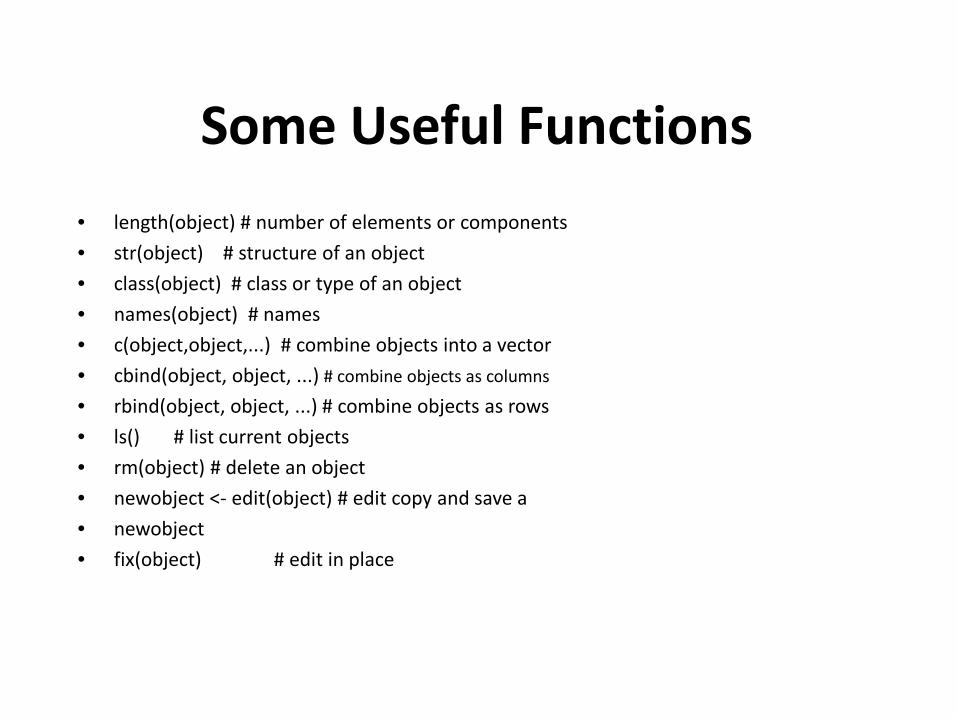
Some Useful Functions • length(object) # number of elements or components • str(object) # structure of an object • class(object) # class or type of an object • names(object) # names • c(object,object,...) # combine objects into a vector • cbind(object, object, ...) # combine objects as columns

• rbind(object, object, ...) # combine objects as rows • ls() # list current objects • rm(object) # delete an object • newobject <- edit(object) # edit copy and save a • newobject • fix(object) # edit in place

R Warning !

R is a case sensitive language. FOO, Foo, and foo are three different objects

Getting Help

> help(t.test) > help.search("standard deviation")

Workspace

R Workspace – Objects that you create during an R session

are hold in memory, the collection of objects that you currently have is called the workspace. This workspace is not saved on disk unless you tell R to do so. This means that your objects are lost when you close R and not save the objects, or worse when R or your system crashes on you during a session.

R Workspace • When you close the RGui or the R console window,

the system will ask if you want to save the workspace image.

• If you select to save the workspace image then all the objects in your current R session are saved in a file .RData.

• This is a binary file located in the working directory of R, which is by default the installation directory of R.

R Workspace • During your R session you can also explicitly save

the workspace image. Go to the `File‘ menu and then select `Save Workspace...', or use the save.image function.

• ## save to the current working directory • save.image() • ## just checking what the current working directory is • getwd() • ## save to a specific file and location • save.image("C:\\Program Files\\R\\R-2.5.0\\bin\\.RData")

R Workspace

• If you have saved a workspace image and you start R the next time, it will restore the workspace. So all your previously saved objects are available again. You can also explicitly load a saved workspace le, that could be the workspace image of someone else. Go the `File' menu and select `Load workspace...'.

R Workspace

# save your command history savehistory(file="myfile") # default is ".Rhistory"

# recall your command history loadhistory(file="myfile") # default is ".Rhistory“

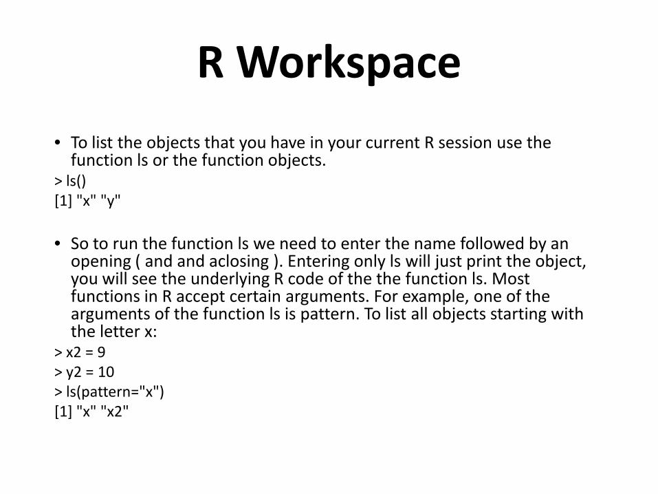
R Workspace • To list the objects that you have in your current R session use the

function ls or the function objects. > ls() [1] "x" "y"

• So to run the function ls we need to enter the name followed by an

opening ( and and aclosing ). Entering only ls will just print the object, you will see the underlying R code of the the function ls. Most functions in R accept certain arguments. For example, one of the arguments of the function ls is pattern. To list all objects starting with the letter x:

> x2 = 9 > y2 = 10 > ls(pattern="x") [1] "x" "x2"

Data Input

Importing From A Comma Delimited Text File

• first row contains variable names, comma is separator • assign the variable id to row names • note the / instead of \ on mswindows systems

mydata <- read.table("c:/mydata.csv", header=TRUE, sep=",", row.names="id")

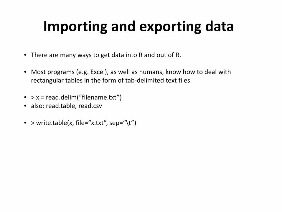
Importing and exporting data

• There are many ways to get data into R and out of R.

• Most programs (e.g. Excel), as well as humans, know how to deal with rectangular tables in the form of tab-delimited text files.

• > x = read.delim(“filename.txt”) • also: read.table, read.csv

• > write.table(x, file=“x.txt”, sep=“\t”)

Reading Data from Files

> myData <- read.table("R_Tutorial_Data.txt", + header=TRUE, sep="\t") > myData Condition Group Pre1 Pre2 Pre3 Pre4 Learning 1 Low A 0.77 0.91 0.24 0.72 0.90 2 Low A 0.82 0.91 0.62 0.90 0.87 3 Low A 0.81 0.70 0.43 0.46 0.90 . . . 61 High B 0.44 0.41 0.84 0.82 0.29 62 High B 0.48 0.56 0.83 0.85 0.48 63 High B 0.61 0.82 0.88 0.95 0.28

Importing data: caveats Type conversions: by default, the read functions try to guess and autoconvert

the data types of the different columns (e.g. number, factor, character). There are options as.is and colClasses to control this – read the online

help Special characters: the delimiter character (space, comma, tabulator) and the

end-of-line character cannot be part of a data field. To circumvent this, text may be “quoted”. However, if this option is used (the default), then the quote characters

themselves cannot be part of a data field. Except if they themselves are within quotes…

Understand the conventions your input files use and set the quote options accordingly.

Keyboard Input

• You can also use R's built in spreadsheet to enter the data interactively, as in the following example.

• # enter data using editor mydata <- data.frame(age=numeric(0), gender=character(0), weight=numeric(0)) mydata <- edit(mydata) # note that without the assignment in the line above, # the edits are not saved!

Keyboard Input

• Usually you will obtain a dataframe by importing it from SAS, SPSS, Excel, Stata, a database, or an ASCII file. To create it interactively, you can do something like the following.

• create a dataframe from scratch age <- c(25, 30, 56) gender <- c("male", "female", "male") weight <- c(160, 110, 220) mydata <- data.frame(age,gender,weight)

Exporting Data

There are numerous methods for exporting R objects into other formats . For SPSS, SAS and Stata. you will need to load the foreign packages. For Excel, you will need the xlsReadWrite package.

Exporting Data

To A Tab Delimited Text File write.table(mydata, "c:/mydata.txt", sep="\t") To an Excel Spreadsheet library(xlsReadWrite)

write.xls(mydata, "c:/mydata.xls") To SAS library(foreign)

write.foreign(mydata, "c:/mydata.txt", "c:/mydata.sas", package="SAS")

Viewing Data There are a number of functions for listing the contents of an object or

dataset. # list objects in the working environment

ls() # list the variables in mydata

names(mydata) # list the structure of mydata

str(mydata) # list levels of factor v1 in mydata

levels(mydata$v1) # dimensions of an object

dim(object)

Viewing Data There are a number of functions for listing the contents of an object or

dataset. # class of an object (numeric, matrix, dataframe, etc)

class(object) # print mydata

mydata # print first 10 rows of mydata

head(mydata, n=10) # print last 5 rows of mydata

tail(mydata, n=5)

Examining datasets

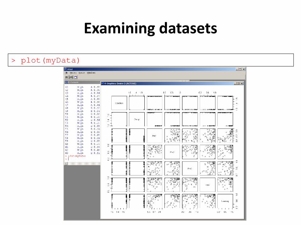
> plot(myData)

Changing the Look of Graphics (I) • The most likely change: orientation and size of labels of x and y axes: > plot(xvalues,yvalues, ylab = "Label for y axis", xlab =

"Label for x axis", las = 1, cex.lab = 1.5)

• ylab, xlab : changes the annotation of the axis labels;

• las : numeric in {0,1,2,3} change orientation of the axis labels; • cex.lab : magnification to be used for x and y labels; • To get full range of changes about graphical parameters: >?par

Working with Data

Selecting Subsets of Data

> myData$Learning [1] 0.90 0.87 0.90 0.85 0.93 0.93 0.89 0.80 0.98 [10] 0.88 0.88 0.94 0.99 0.92 0.83 0.65 0.57 0.55 [19] 0.94 0.68 0.89 0.60 0.63 0.84 0.92 0.56 0.78 [28] 0.54 0.47 0.45 0.59 0.91 0.98 0.82 0.93 0.81 [37] 0.97 0.95 0.70 1.00 0.90 0.99 0.95 0.95 0.97 [46] 1.00 0.99 0.18 0.33 0.88 0.23 0.75 0.21 0.35 [55] 0.70 0.34 0.43 0.75 0.44 0.44 0.29 0.48 0.28 > myData$Learning[myData$Group=="A"] [1] 0.90 0.87 0.90 0.85 0.93 0.93 0.89 0.80 0.98 [10] 0.88 0.88 0.94 0.99 0.92 0.83 0.65 0.98 0.82 [19] 0.93 0.81 0.97 0.95 0.70 1.00 0.90 0.99 0.95 [28] 0.95 0.97 1.00 0.99

Selecting Subsets of Data

> myData$Learning [1] 0.90 0.87 0.90 0.85 0.93 0.93 0.89 0.80 0.98 [10] 0.88 0.88 0.94 0.99 0.92 0.83 0.65 0.57 0.55 [19] 0.94 0.68 0.89 0.60 0.63 0.84 0.92 0.56 0.78 [28] 0.54 0.47 0.45 0.59 0.91 0.98 0.82 0.93 0.81 [37] 0.97 0.95 0.70 1.00 0.90 0.99 0.95 0.95 0.97 [46] 1.00 0.99 0.18 0.33 0.88 0.23 0.75 0.21 0.35 [55] 0.70 0.34 0.43 0.75 0.44 0.44 0.29 0.48 0.28 > attach(myData) > Learning [1] 0.90 0.87 0.90 0.85 0.93 0.93 0.89 0.80 0.98 [10] 0.88 0.88 0.94 0.99 0.92 0.83 0.65 0.57 0.55 [19] 0.94 0.68 0.89 0.60 0.63 0.84 0.92 0.56 0.78 [28] 0.54 0.47 0.45 0.59 0.91 0.98 0.82 0.93 0.81 [37] 0.97 0.95 0.70 1.00 0.90 0.99 0.95 0.95 0.97 [46] 1.00 0.99 0.18 0.33 0.88 0.23 0.75 0.21 0.35 [55] 0.70 0.34 0.43 0.75 0.44 0.44 0.29 0.48 0.28

> Learning[Group=="A"] [1] 0.90 0.87 0.90 0.85 0.93 0.93 0.89 0.80 0.98 [10] 0.88 0.88 0.94 0.99 0.92 0.83 0.65 0.98 0.82 [19] 0.93 0.81 0.97 0.95 0.70 1.00 0.90 0.99 0.95 [28] 0.95 0.97 1.00 0.99 > Learning[Group!="A"] [1] 0.57 0.55 0.94 0.68 0.89 0.60 0.63 0.84 0.92 [10] 0.56 0.78 0.54 0.47 0.45 0.59 0.91 0.18 0.33 [19] 0.88 0.23 0.75 0.21 0.35 0.70 0.34 0.43 0.75 [28] 0.44 0.44 0.29 0.48 0.28 > Condition[Group=="B"&Learning<0.5] [1] Low Low High High High High High High High [10] High High High High High Levels: High Low

Selecting Subsets of Data

Storing data • Every R object can be stored into and restored from a file with the commands

“save” and “load”. • This uses the XDR (external data representation) standard of Sun Microsystems

and others, and is portable between MS-Windows, Unix, Mac. > save(x, file=“x.Rdata”) > load(“x.Rdata”)

Dataframes • R handles data in objects known as dataframes;

– rows: different observations; – columns: values of the different variables (numbers,

text, calendar dates or logical variables (T or F);

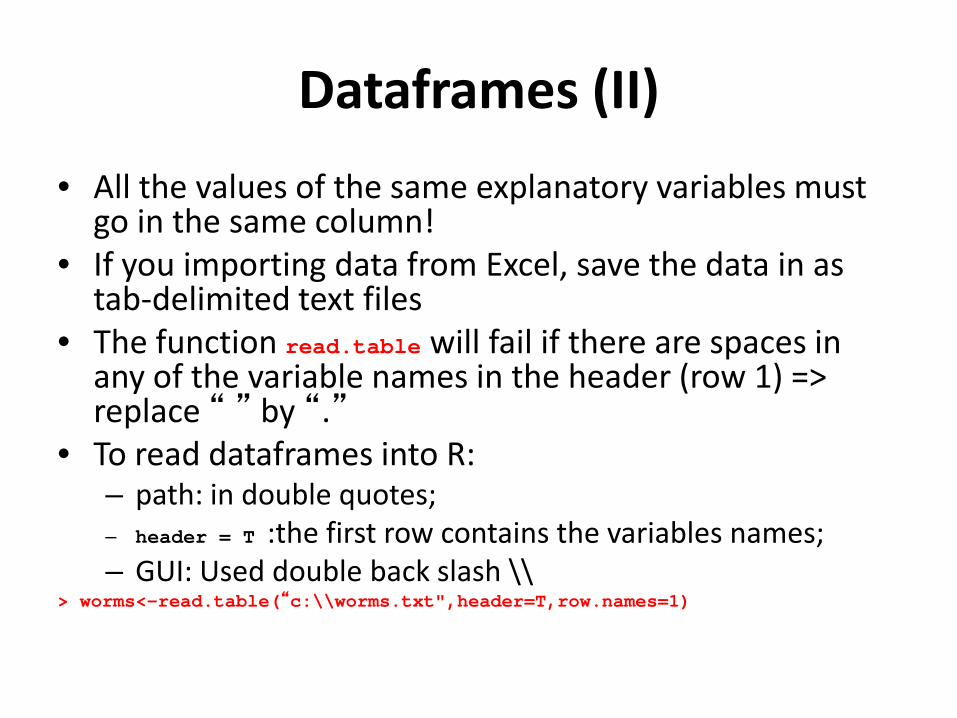
Dataframes (II) • All the values of the same explanatory variables must

go in the same column! • If you importing data from Excel, save the data in as

tab-delimited text files • The function read.table will fail if there are spaces in

any of the variable names in the header (row 1) => replace “ ” by “.”

• To read dataframes into R: – path: in double quotes; – header = T :the first row contains the variables names; – GUI: Used double back slash \\

> worms<-read.table(“c:\\worms.txt",header=T,row.names=1)

Dataframes (III)

• Use attach to make the variables accessible by name:

> attach(worms)

• Use names to get a list of variable names: > names(worms) [1] "Area" "Slope" "Vegetation"

"Soil.pH" "Damp" [6] "Worm.density“

• To see the content of the dataframe (object) just type ist name:

> worms

Dataframes (III) • Summary(worms)

Area Slope Vegetation Soil.pH Damp Worm.density

Min. :0.800 Min. : 0.00 Arable :3 Min. :3.500 Mode :logical Min. :0.00 1st Qu.:2.175 1st Qu.: 0.75 Grassland:9 1st Qu.:4.100 FALSE:14 1st Qu.:2.00 Median :3.000 Median : 2.00 Meadow :3 Median :4.600 TRUE :6 Median :4.00 Mean :2.990 Mean : 3.50 Orchard :1 Mean :4.555 Mean :4.35 3rd Qu.:3.725 3rd Qu.: 5.25 Scrub :4 3rd Qu.:5.000 3rd Qu.:6.25 Max. :5.100 Max. :11.00 Max. :5.700 Max. :9.00

• Values of the continuous variables: – arithmetic mean; – maximum, minimum, median, 25 and 75 percentiles

(first and third quartile); • Levels of categorical variables are counted

Selecting Parts of a Dataframe: Subscripts

• Subscripts within square brackets: to select part of a dataframe

• [, means “all the rows” and ,] means “all the columns”

• To select the first three column of the dataframe worms:

> worms[,1:3]

Area Slope Vegetation Nashs.Field 3.6 11 Grassland Silwood.Bottom 5.1 2 Arable Nursery.Field 2.8 3 Grassland Rush.Meadow 2.4 5 Meadow Gunness.Thicket 3.8 0 Scrub (…)

Selecting Parts of a Dataframe: Subscripts (II)

• To select certain rows based on logical tests on the values of one or more variables:

> worms[Area>3&Slope<3,]

Area Slope Vegetation Soil.pH Damp Worm.density Silwood.Bottom 5.1 2 Arable 5.2 FALSE 7 Gunness.Thicket 3.8 0 Scrub 4.2 FALSE 6 Oak.Mead 3.1 2 Grassland 3.9 FALSE 2 North.Gravel 3.3 1 Grassland 4.1 FALSE 1 South.Gravel 3.7 2 Grassland 4.0 FALSE 2 Pond.Field 4.1 0 Meadow 5.0 TRUE 6 Water.Meadow 3.9 0 Meadow 4.9 TRUE 8 Pound.Hill 4.4 2 Arable 4.5 FALSE 5

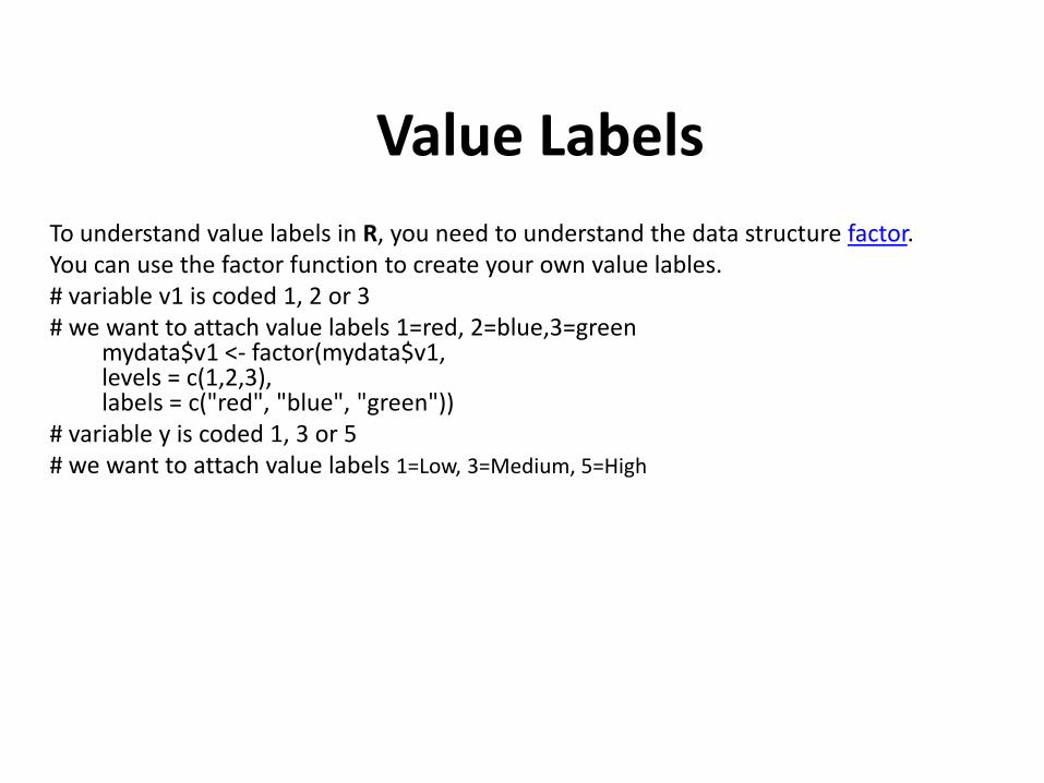
Value Labels To understand value labels in R, you need to understand the data structure factor. You can use the factor function to create your own value lables. # variable v1 is coded 1, 2 or 3 # we want to attach value labels 1=red, 2=blue,3=green

mydata$v1 <- factor(mydata$v1, levels = c(1,2,3), labels = c("red", "blue", "green"))

# variable y is coded 1, 3 or 5 # we want to attach value labels 1=Low, 3=Medium, 5=High

Value Labels mydata$v1 <- ordered(mydata$y,

levels = c(1,3, 5), labels = c("Low", "Medium", "High"))

Use the factor() function for nominal data and the ordered() function for ordinal data. R statistical and graphic functions will then treat the data appropriately.

Note: factor and ordered are used the same way, with the same arguments. The former creates factors and the later creates ordered factors.

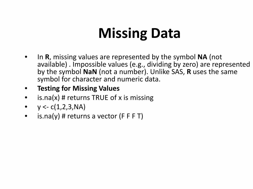
Missing Data • In R, missing values are represented by the symbol NA (not

available) . Impossible values (e.g., dividing by zero) are represented by the symbol NaN (not a number). Unlike SAS, R uses the same symbol for character and numeric data.

• Testing for Missing Values • is.na(x) # returns TRUE of x is missing • y <- c(1,2,3,NA) • is.na(y) # returns a vector (F F F T)

Missing Data • Recoding Values to Missing

– # recode 99 to missing for variable v1 – # select rows where v1 is 99 and recode column v1 – mydata[mydata$v1==99,"v1"] <- NA

• Excluding Missing Values from Analyses – Arithmetic functions on missing values yield missing values. – x <- c(1,2,NA,3) – mean(x) # returns NA – mean(x, na.rm=TRUE) # returns 2

Missing Data • The function complete.cases() returns a logical vector

indicating which cases are complete. – list rows of data that have missing values

mydata[!complete.cases(mydata),] • The function na.omit() returns the object with listwise

deletion of missing values. – create new dataset without missing data

newdata <- na.omit(mydata)

Date Values Dates are represented as the number of days since 1970-01-01, with

negative values for earlier dates. # use as.Date( ) to convert strings to dates mydates <- as.Date(c("2007-06-22", "2004-02-13")) # number of days between 6/22/07 and 2/13/04

days <- mydates[1] - mydates[2] Sys.Date( ) returns today's date. Date() returns the current date and time.

Date Values The following symbols can be used with the format( )

function to print dates. Symbol Meaning Example

%d day as a number (0-31) 01-31

%a %A

abbreviated weekday unabbreviated weekday

Mon Monday

%m month (00-12) 00-12

%b %B

abbreviated month unabbreviated month

Jan January

%y %Y

2-digit year 4-digit year

07 2007

Date Values # print today's date today <- Sys.Date() format(today, format="%B %d %Y")

"June 20 2007"

Variables, Lists, and Arrays

Object orientation

primitive (or: atomic) data types in R are:

• numeric (integer, double, complex) • character • logical • function

out of these, vectors, arrays, lists can be built.

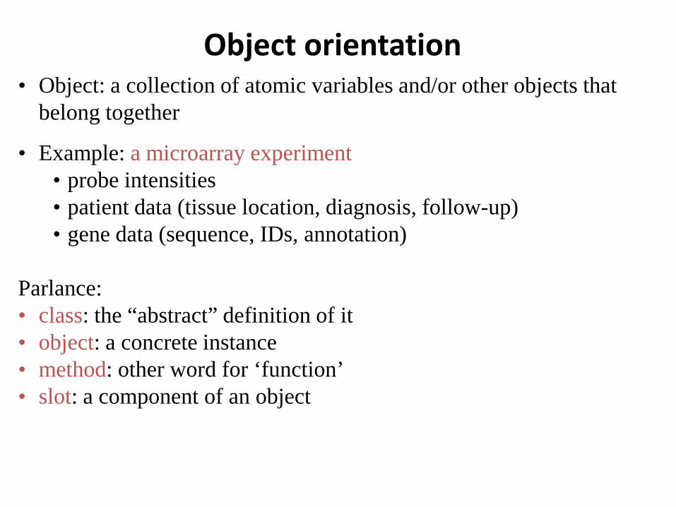
Object orientation • Object: a collection of atomic variables and/or other objects that

belong together

• Example: a microarray experiment • probe intensities • patient data (tissue location, diagnosis, follow-up) • gene data (sequence, IDs, annotation)

Parlance: • class: the “abstract” definition of it • object: a concrete instance • method: other word for ‘function’ • slot: a component of an object

Object orientation Advantages:

Encapsulation (can use the objects and methods someone else has written without having to care about the internals)

Generic functions (e.g. plot, print)

Inheritance (hierarchical organization of complexity)

Caveat: Overcomplicated, baroque program architecture…

Variables > a = 49 > sqrt(a) [1] 7

> a = "The dog ate my homework" > sub("dog","cat",a) [1] "The cat ate my homework“ > a = (1+1==3) > a [1] FALSE

numeric

character string

logical

Variable Labels R's ability to handle variable labels is somewhat

unsatisfying. If you use the Hmisc package, you can take advantage of

some labeling features. library(Hmisc)

label(mydata$myvar) <- "Variable label for variable myvar" describe(mydata)

Variable Labels Unfortunately the label is only in effect for functions provided by

the Hmisc package, such as describe(). Your other option is to use the variable label as the variable name and then refer to the variable by position index.

names(mydata)[3] <- "This is the label for variable 3" mydata[3] # list the variable

Vectors, matrices and arrays • vector: an ordered collection of data of the same type > a = c(1,2,3) > a*2 [1] 2 4 6 • Example: the mean spot intensities of all 15488 spots on a chip: a vector of 15488

numbers • In R, a single number is the special case of a vector with 1 element.

• Other vector types: character strings, logical

Vectors, matrices and arrays

• matrix: a rectangular table of data of the same type • example: the expression values for 10000 genes for 30 tissue biopsies: a matrix with

10000 rows and 30 columns. • array: 3-,4-,..dimensional matrix

• example: the red and green foreground and background values for 20000 spots on 120 chips: a 4 x 20000 x 120 (3D) array.

Subscripts: Obtaining Parts of Vectors

• Elements of vectors by subscripts in []: > y[3]

• The third to the seventh elements of y: > y[3:7]

• The third, fifth, sixth and ninth elements: > y[c(3,5,6,7)]

• To drop an element from the array, use negative subscripts:

> y[-1]

• To drop the last element of the array without knowing its length:

> y[-length(y)]

Subscripts as Logical Variables

• Logical condition to find a subset of the values in a vector:

> y[y>6]

• To know the values for z for wich y>6: > z[y>6]

• Element of y not multiples of three: > y[y%%3!=0]

Subscripts with Arrays (I) • Three-dimensional array containing the numbers 1 to 30, with five rows and three

columns in each two tables: > A<-array(1:30,c(5,3,2)) > A , , 1 [,1] [,2] [,3] The numbers enter each table [1,] 1 6 11 column-wise, from left to right [2,] 2 7 12 (rows, then columns then tables) [3,] 3 8 13 [4,] 4 9 14 [5,] 5 10 15

, , 2

[,1] [,2] [,3] [1,] 16 21 26 [2,] 17 22 27 [3,] 18 23 28 [4,] 19 24 29 [5,] 20 25 30

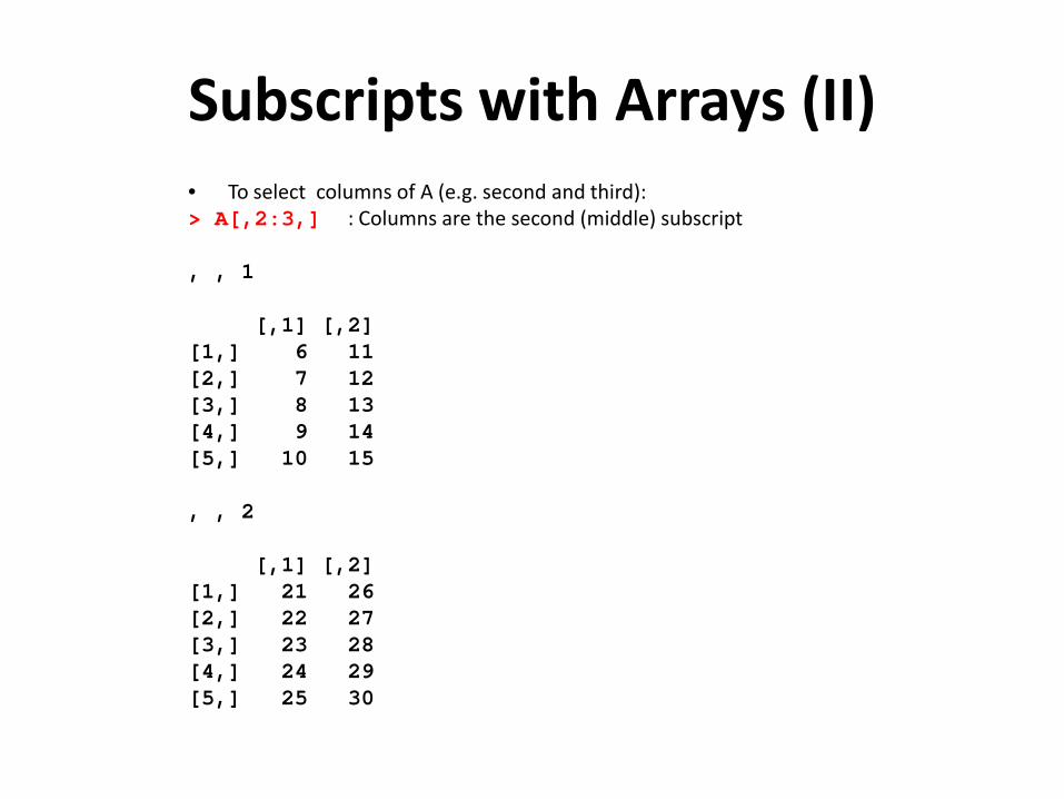
Subscripts with Arrays (II) • To select columns of A (e.g. second and third): > A[,2:3,] : Columns are the second (middle) subscript , , 1 [,1] [,2] [1,] 6 11 [2,] 7 12 [3,] 8 13 [4,] 9 14 [5,] 10 15

, , 2

[,1] [,2] [1,] 21 26 [2,] 22 27 [3,] 23 28 [4,] 24 29 [5,] 25 30

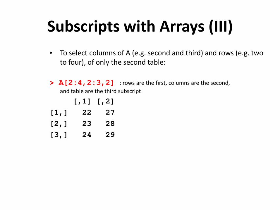
Subscripts with Arrays (III) • To select columns of A (e.g. second and third) and rows (e.g. two

to four), of only the second table:

> A[2:4,2:3,2] : rows are the first, columns are the second, and table are the third subscript

[,1] [,2] [1,] 22 27 [2,] 23 28 [3,] 24 29

Lists • vector: an ordered collection of data of the same type. > a = c(7,5,1) > a[2] [1] 5 • list: an ordered collection of data of arbitrary types. > doe = list(name="john",age=28,married=F) > doe$name [1] "john“ > doe$age [1] 28 • Typically, vector elements are accessed by their index (an integer), list elements by their

name (a character string). But both types support both access methods.

Installing, Running, and Interacting with R

> 1 + 1 [1] 2 > 1 + 1 * 7 [1] 8 > (1 + 1) * 7 [1] 14

> x <- 1 > x [1] 1 > y = 2 > y [1] 2 > 3 -> z > z [1] 3 > (x + y) * z [1] 9

Math: Variables:

Installing, Running, and Interacting with R

> x <- c(0,1,2,3,4) > x [1] 0 1 2 3 4 > y <- 1:5 > y [1] 1 2 3 4 5 > z <- 1:50 > z [1] 1 2 3 4 5 6 7 8 9 10 11 12 13 14 15 [16] 16 17 18 19 20 21 22 23 24 25 26 27 28 29 30 [31] 31 32 33 34 35 36 37 38 39 40 41 42 43 44 45 [46] 46 47 48 49 50

Arrays:

Installing, Running, and Interacting with R

> x <- c(0,1,2,3,4) > y <- 1:5 > z <- 1:50 > x + y [1] 1 3 5 7 9 > x * y [1] 0 2 6 12 20 > x * z [1] 0 2 6 12 20 0 7 16 27 40 0 [12] 12 26 42 60 0 17 36 57 80 0 22 [23] 46 72 100 0 27 56 87 120 0 32 66 [34] 102 140 0 37 76 117 160 0 42 86 132 [45] 180 0 47 96 147 200

Math on arrays:

Functions

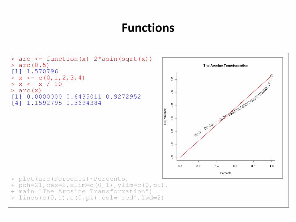
> arc <- function(x) 2*asin(sqrt(x)) > arc(0.5) [1] 1.570796 > x <- c(0,1,2,3,4) > x <- x / 10 > arc(x) [1] 0.0000000 0.6435011 0.9272952 [4] 1.1592795 1.3694384 > plot(arc(Percents)~Percents, + pch=21,cex=2,xlim=c(0,1),ylim=c(0,pi), + main="The Arcsine Transformation") > lines(c(0,1),c(0,pi),col="red",lwd=2)

R Packages

– One of the strengths of R is that the system can easily be extended. The system allows you to write new functions and package those functions in a so called `R package' (or `R library'). The R package may also contain other R objects, for example data sets or documentation. There is a lively R user community and many R packages have been written and made available on CRAN for other users. Just a few examples, there are packages for portfolio optimization, drawing maps, exporting objects to html, time series analysis, spatial statistics and the list goes on and on.

R Packages

– To attach another package to the system you can use the menu or the library function. Via the menu: Select the `Packages' menu and select `Load package...', a list of available packages on your system will be displayed. Select one and click `OK', the package is now attached to your current R session. Via the library function: > library(MASS) > shoes $A [1] 13.2 8.2 10.9 14.3 10.7 6.6 9.5 10.8 8.8 13.3 $B [1] 14.0 8.8 11.2 14.2 11.8 6.4 9.8 11.3 9.3 13.6

Data Manipulation

Outline • Creating New Variable • Operators • Built-in functions • Control Structures • User Defined Functions • Sorting Data • Merging Data • Aggregating Data • Reshaping Data • Sub-setting Data • Data Type Conversions

Introduction

Once you have access to your data, you will want to massage it into useful form. This includes creating new variables (including recoding and renaming existing variables), sorting and merging datasets, aggregating data, reshaping data, and subsetting datasets (including selecting observations that meet criteria, randomly sampling observation, and dropping or keeping variables).

Introduction

Each of these activities usually involve the use of R's built-in operators (arithmetic and logical) and functions (numeric, character, and statistical). Additionally, you may need to use control structures (if-then, for, while, switch) in your programs and/or create your own functions. Finally you may need to convert variables or datasets from one type to another (e.g. numeric to character or matrix to dataframe).

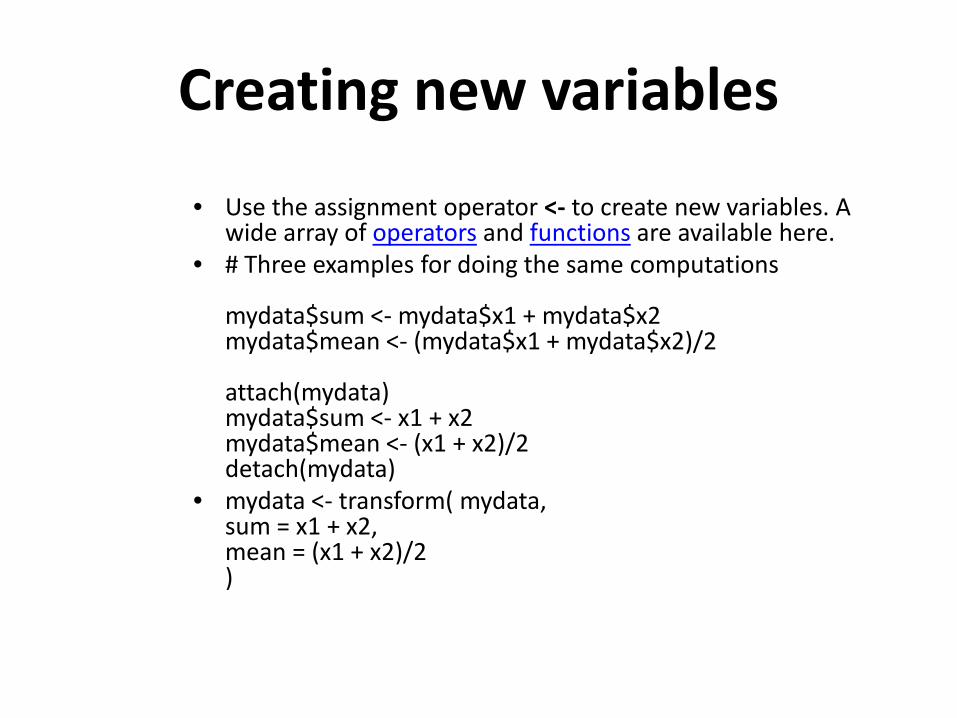
Creating new variables

• Use the assignment operator <- to create new variables. A wide array of operators and functions are available here.

• # Three examples for doing the same computations mydata$sum <- mydata$x1 + mydata$x2 mydata$mean <- (mydata$x1 + mydata$x2)/2 attach(mydata) mydata$sum <- x1 + x2 mydata$mean <- (x1 + x2)/2 detach(mydata)

• mydata <- transform( mydata, sum = x1 + x2, mean = (x1 + x2)/2 )

Creating new variables

Recoding variables • In order to recode data, you will probably use one or

more of R's control structures. • # create 2 age categories

mydata$agecat <- ifelse(mydata$age > 70, c("older"), c("younger")) # another example: create 3 age categories attach(mydata) mydata$agecat[age > 75] <- "Elder" mydata$agecat[age > 45 & age <= 75] <- "Middle Aged" mydata$agecat[age <= 45] <- "Young" detach(mydata)

Creating new variables

Recoding variables • In order to recode data, you will probably use one or more of

R's control structures. • # create 2 age categories

mydata$agecat <- ifelse(mydata$age > 70, c("older"), c("younger")) # another example: create 3 age categories attach(mydata) mydata$agecat[age > 75] <- "Elder" mydata$agecat[age > 45 & age <= 75] <- "Middle Aged" mydata$agecat[age <= 45] <- "Young" detach(mydata)

Creating new variables

Renaming variables • You can rename variables programmatically or interactively. • # rename interactively

fix(mydata) # results are saved on close # rename programmatically library(reshape) mydata <- rename(mydata, c(oldname="newname")) # you can re-enter all the variable names in order # changing the ones you need to change.the limitation # is that you need to enter all of them! names(mydata) <- c("x1","age","y", "ses")

Arithmetic Operators

Operator Description + addition - subtraction * multiplication / division ^ or ** exponentiation x %% y modulus (x mod y) 5%%2 is 1 x %/% y integer division 5%/%2 is 2

Logical Operators

Operator Description < less than <= less than or equal to > greater than >= greater than or equal to == exactly equal to != not equal to !x Not x x | y x OR y x & y x AND y isTRUE(x) test if x is TRUE

Control Structures

• R has the standard control structures you would expect. expr can be multiple (compound) statements by enclosing them in braces { }. It is more efficient to use built-in functions rather than control structures whenever possible.

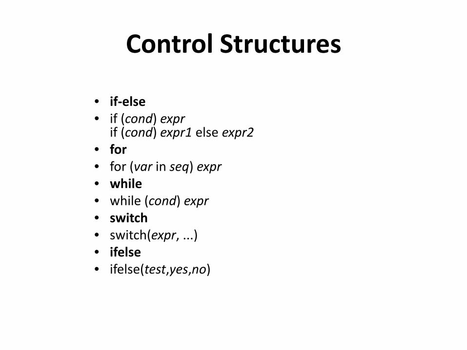
Control Structures

• if-else • if (cond) expr

if (cond) expr1 else expr2 • for • for (var in seq) expr • while • while (cond) expr • switch • switch(expr, ...) • ifelse • ifelse(test,yes,no)

Control Structures

• # transpose of a matrix # a poor alternative to built-in t() function mytrans <- function(x) { if (!is.matrix(x)) { warning("argument is not a matrix: returning NA") return(NA_real_) } y <- matrix(1, nrow=ncol(x), ncol=nrow(x)) for (i in 1:nrow(x)) { for (j in 1:ncol(x)) { y[j,i] <- x[i,j] } } return(y) }

Control Structures

• # try it z <- matrix(1:10, nrow=5, ncol=2) tz <- mytrans(z)

R built-in functions

Almost everything in R is done through functions. Here I'm only referring to numeric and character functions that are commonly used in creating or recoding variables. Note that while the examples on this page apply functions to individual variables, many can be applied to vectors and matrices as well.

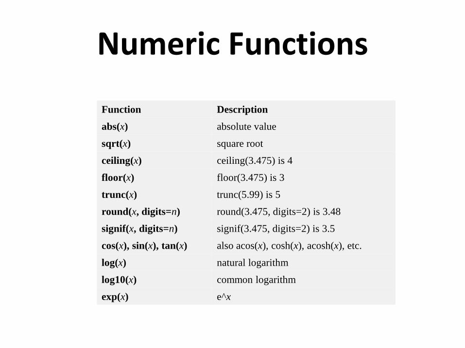
Numeric Functions

Function Description abs(x) absolute value sqrt(x) square root ceiling(x) ceiling(3.475) is 4 floor(x) floor(3.475) is 3 trunc(x) trunc(5.99) is 5 round(x, digits=n) round(3.475, digits=2) is 3.48 signif(x, digits=n) signif(3.475, digits=2) is 3.5 cos(x), sin(x), tan(x) also acos(x), cosh(x), acosh(x), etc. log(x) natural logarithm log10(x) common logarithm exp(x) e^x

Character Functions

Function Description

substr(x, start=n1, stop=n2) Extract or replace substrings in a character vector. x <- "abcdef" substr(x, 2, 4) is "bcd" substr(x, 2, 4) <- "22222" is "a222ef"

grep(pattern, x , ignore.case=FALSE, fixed=FALSE)

Search for pattern in x. If fixed =FALSE then pattern is a regular expression. If fixed=TRUE then pattern is a text string. Returns matching indices. grep("A", c("b","A","c"), fixed=TRUE) returns 2

sub(pattern, replacement, x, ignore.case =FALSE, fixed=FALSE)

Find pattern in x and replace with replacement text. If fixed=FALSE then pattern is a regular expression. If fixed = T then pattern is a text string. sub("\\s",".","Hello There") returns "Hello.There"

strsplit(x, split) Split the elements of character vector x at split. strsplit("abc", "") returns 3 element vector "a","b","c"

paste(..., sep="") Concatenate strings after using sep string to seperate them. paste("x",1:3,sep="") returns c("x1","x2" "x3") paste("x",1:3,sep="M") returns c("xM1","xM2" "xM3") paste("Today is", date())

toupper(x) Uppercase

tolower(x) Lowercase

Stat/Prob Functions • The following table describes functions related to

probaility distributions. For random number generators below, you can use set.seed(1234) or some other integer to create reproducible pseudo-random numbers.

Function Description

dnorm(x) normal density function (by default m=0 sd=1) # plot standard normal curve x <- pretty(c(-3,3), 30) y <- dnorm(x) plot(x, y, type='l', xlab="Normal Deviate", ylab="Density", yaxs="i")

pnorm(q) cumulative normal probability for q (area under the normal curve to the right of q) pnorm(1.96) is 0.975

qnorm(p) normal quantile. value at the p percentile of normal distribution qnorm(.9) is 1.28 # 90th percentile

rnorm(n, m=0,sd=1) n random normal deviates with mean m and standard deviation sd. #50 random normal variates with mean=50, sd=10 x <- rnorm(50, m=50, sd=10)

dbinom(x, size, prob) pbinom(q, size, prob) qbinom(p, size, prob) rbinom(n, size, prob)

binomial distribution where size is the sample size and prob is the probability of a heads (pi) # prob of 0 to 5 heads of fair coin out of 10 flips dbinom(0:5, 10, .5) # prob of 5 or less heads of fair coin out of 10 flips pbinom(5, 10, .5)

dpois(x, lamda) ppois(q, lamda) qpois(p, lamda) rpois(n, lamda)

poisson distribution with m=std=lamda #probability of 0,1, or 2 events with lamda=4 dpois(0:2, 4) # probability of at least 3 events with lamda=4 1- ppois(2,4)

dunif(x, min=0, max=1) punif(q, min=0, max=1) qunif(p, min=0, max=1) runif(n, min=0, max=1)

uniform distribution, follows the same pattern as the normal distribution above. #10 uniform random variates x <- runif(10)

Function Description

mean(x, trim=0, na.rm=FALSE)

mean of object x # trimmed mean, removing any missing values and # 5 percent of highest and lowest scores mx <- mean(x,trim=.05,na.rm=TRUE)

sd(x) standard deviation of object(x). also look at var(x) for variance and mad(x) for median absolute deviation.

median(x) median

quantile(x, probs) quantiles where x is the numeric vector whose quantiles are desired and probs is a numeric vector with probabilities in [0,1]. # 30th and 84th percentiles of x y <- quantile(x, c(.3,.84))

range(x) range

sum(x) sum

diff(x, lag=1) lagged differences, with lag indicating which lag to use

min(x) minimum

max(x) maximum

scale(x, center=TRUE, scale=TRUE)

column center or standardize a matrix.

Other Useful Functions

Function Description

seq(from , to, by) generate a sequence indices <- seq(1,10,2) #indices is c(1, 3, 5, 7, 9)

rep(x, ntimes) repeat x n times y <- rep(1:3, 2) # y is c(1, 2, 3, 1, 2, 3)

cut(x, n) divide continuous variable in factor with n levels y <- cut(x, 5)

Sorting • To sort a dataframe in R, use the order( ) function. By default,

sorting is ASCENDING. Prepend the sorting variable by a minus sign to indicate DESCENDING order. Here are some examples.

• # sorting examples using the mtcars dataset data(mtcars) # sort by mpg newdata = mtcars[order(mtcars$mpg),] # sort by mpg and cyl newdata <- mtcars[order(mtcars$mpg, mtcars$cyl),] #sort by mpg (ascending) and cyl (descending) newdata <- mtcars[order(mtcars$mpg, -mtcars$cyl),]

Merging To merge two dataframes (datasets) horizontally, use the merge

function. In most cases, you join two dataframes by one or more common key variables (i.e., an inner join).

# merge two dataframes by ID total <- merge(dataframeA,dataframeB,by="ID")

# merge two dataframes by ID and Country total <- merge(dataframeA,dataframeB,by=c("ID","Country"))

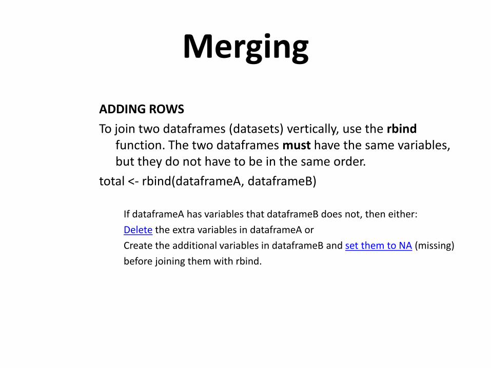
Merging ADDING ROWS To join two dataframes (datasets) vertically, use the rbind

function. The two dataframes must have the same variables, but they do not have to be in the same order.

total <- rbind(dataframeA, dataframeB) If dataframeA has variables that dataframeB does not, then either: Delete the extra variables in dataframeA or Create the additional variables in dataframeB and set them to NA (missing) before joining them with rbind.

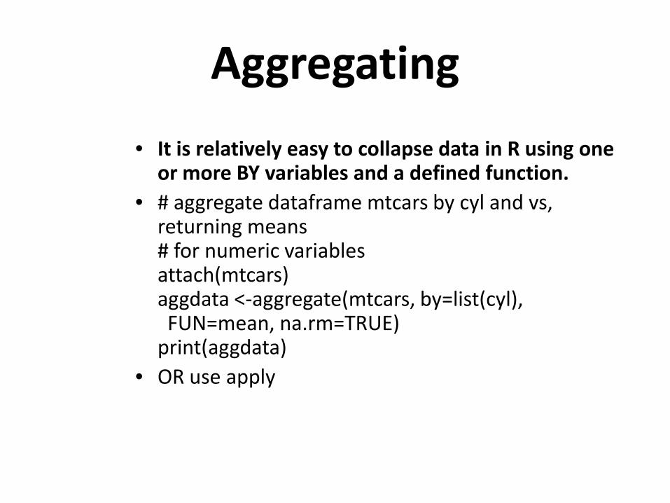
Aggregating • It is relatively easy to collapse data in R using one

or more BY variables and a defined function. • # aggregate dataframe mtcars by cyl and vs,

returning means # for numeric variables attach(mtcars) aggdata <-aggregate(mtcars, by=list(cyl), FUN=mean, na.rm=TRUE) print(aggdata)

• OR use apply

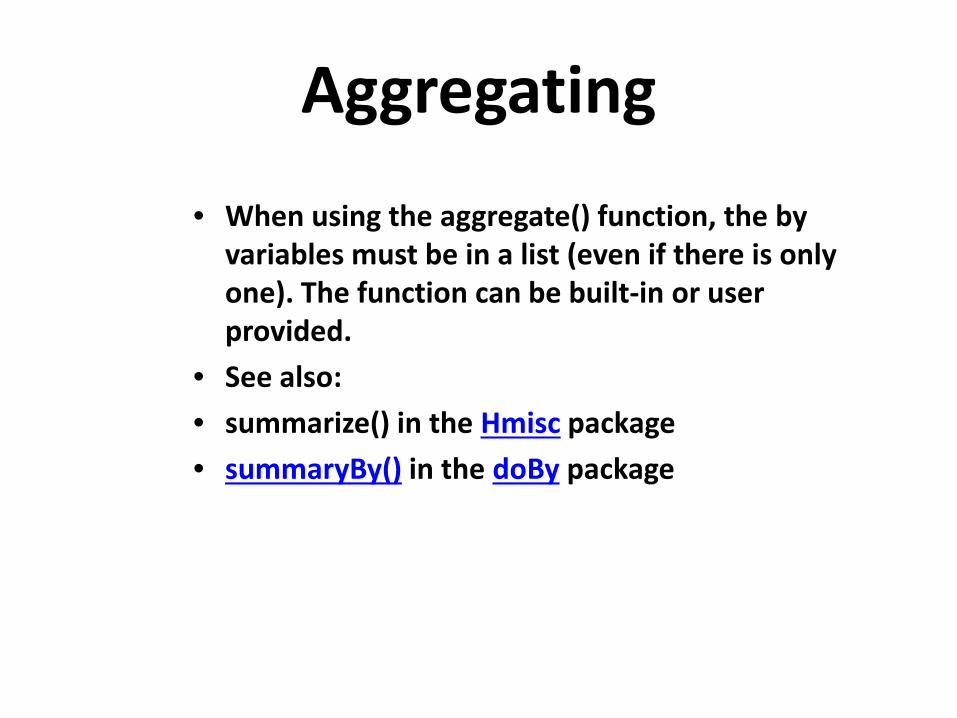
Aggregating • When using the aggregate() function, the by

variables must be in a list (even if there is only one). The function can be built-in or user provided.

• See also: • summarize() in the Hmisc package • summaryBy() in the doBy package

Data Type Conversion

• Type conversions in R work as you would expect. For example, adding a character string to a numeric vector converts all the elements in the vector to character.

• Use is.foo to test for data type foo. Returns TRUE or FALSE Use as.foo to explicitly convert it.

• is.numeric(), is.character(), is.vector(), is.matrix(), is.data.frame() as.numeric(), as.character(), as.vector(), as.matrix(), as.data.frame)