Embed Size (px)
Citation preview

A Tutorial on MIMO
Craig WilsonEE381K-11: Wireless Communications
Spring 2009
May 9, 2009

Contents
1 Introduction 1
2 Benefits of MIMO 1
2.1 Diversity . . . . . . . . . . . . . . . . . . . . . . . . . . . . . . . . . . . . . . . . 2
2.1.1 Union Bound on Probability of Error . . . . . . . . . . . . . . . . . . . . 3
2.1.2 Outage Probability . . . . . . . . . . . . . . . . . . . . . . . . . . . . . . 4
2.2 Spatial Multiplexing . . . . . . . . . . . . . . . . . . . . . . . . . . . . . . . . . 5
3 Basic Schemes for Multiple Antennas 5
3.1 Channel Models . . . . . . . . . . . . . . . . . . . . . . . . . . . . . . . . . . . . 5
3.2 Scalar Rayleigh Channel . . . . . . . . . . . . . . . . . . . . . . . . . . . . . . . 6
3.3 Maximal Ratio Combining . . . . . . . . . . . . . . . . . . . . . . . . . . . . . . 6
3.4 Selection Combining . . . . . . . . . . . . . . . . . . . . . . . . . . . . . . . . . 7
3.5 Equal Gain Combining . . . . . . . . . . . . . . . . . . . . . . . . . . . . . . . . 8
3.6 Transmit Maximal Ratio Combining . . . . . . . . . . . . . . . . . . . . . . . . 8
3.7 Alamouti Code . . . . . . . . . . . . . . . . . . . . . . . . . . . . . . . . . . . . 9
4 MIMO Channel Modeling and Capacity 10
4.1 Narrowband MIMO Channel . . . . . . . . . . . . . . . . . . . . . . . . . . . . . 11
4.1.1 Narrowband MIMO Channel Capacity . . . . . . . . . . . . . . . . . . . 11
4.1.2 Rank and Condition Number . . . . . . . . . . . . . . . . . . . . . . . . 12
4.2 Physical Modeling of MIMO Channels . . . . . . . . . . . . . . . . . . . . . . . 12
4.2.1 LOS SIMO and MISO Channel . . . . . . . . . . . . . . . . . . . . . . . 13
4.2.2 LOS MIMO . . . . . . . . . . . . . . . . . . . . . . . . . . . . . . . . . . 15
4.2.3 Geographically Separated MIMO . . . . . . . . . . . . . . . . . . . . . . 15
4.2.4 Two-Ray MIMO . . . . . . . . . . . . . . . . . . . . . . . . . . . . . . . 16
4.3 Statistical Modeling of MIMO Channels . . . . . . . . . . . . . . . . . . . . . . 17
4.3.1 Frequency Selective MIMO Channel . . . . . . . . . . . . . . . . . . . . . 19
i

5 Diversity-Multiplexing Tradeoff 20
5.1 Scalar Rayleigh Channel . . . . . . . . . . . . . . . . . . . . . . . . . . . . . . . 20
5.1.1 QAM over the Scalar Rayleigh Channel . . . . . . . . . . . . . . . . . . . 21
5.2 MISO Rayleigh Channel . . . . . . . . . . . . . . . . . . . . . . . . . . . . . . . 21
5.3 MIMO Rayleigh Channel . . . . . . . . . . . . . . . . . . . . . . . . . . . . . . . 21
6 Space-Time Coding over Narrowband Channels 23
6.1 Error Motivated Design . . . . . . . . . . . . . . . . . . . . . . . . . . . . . . . 24
6.2 Space-Time Block Codes . . . . . . . . . . . . . . . . . . . . . . . . . . . . . . . 25
6.2.1 Linear STBCs . . . . . . . . . . . . . . . . . . . . . . . . . . . . . . . . . 26
6.3 Bell Labs Space Time Architectures . . . . . . . . . . . . . . . . . . . . . . . . . 30
6.3.1 V-BLAST . . . . . . . . . . . . . . . . . . . . . . . . . . . . . . . . . . . 31
6.3.2 D-BLAST . . . . . . . . . . . . . . . . . . . . . . . . . . . . . . . . . . . 38
6.4 Space-Time Trellis Codes . . . . . . . . . . . . . . . . . . . . . . . . . . . . . . . 39
6.4.1 Trellis Representation . . . . . . . . . . . . . . . . . . . . . . . . . . . . 39
6.4.2 Delay-Diversity Scheme . . . . . . . . . . . . . . . . . . . . . . . . . . . . 40
7 Space-Time Coding for Frequency Selective Channels 40
7.1 Single Carrier . . . . . . . . . . . . . . . . . . . . . . . . . . . . . . . . . . . . . 40
7.2 MIMO-OFDM . . . . . . . . . . . . . . . . . . . . . . . . . . . . . . . . . . . . . 41
7.2.1 OFDM . . . . . . . . . . . . . . . . . . . . . . . . . . . . . . . . . . . . . 41
7.2.2 Extension to MIMO-OFDM . . . . . . . . . . . . . . . . . . . . . . . . . 42
7.2.3 Space-Frequency Coded MIMO-OFDM . . . . . . . . . . . . . . . . . . . 43
7.2.4 Space-Time Coded MIMO-OFDM . . . . . . . . . . . . . . . . . . . . . . 43
7.2.5 Space-Time Frequency Coded MIMO-OFDM . . . . . . . . . . . . . . . . 44
8 Multiuser MIMO 44
8.1 Precoding . . . . . . . . . . . . . . . . . . . . . . . . . . . . . . . . . . . . . . . 45
8.1.1 Linear Precoding . . . . . . . . . . . . . . . . . . . . . . . . . . . . . . . 45
8.1.2 Nonlinear Precoding . . . . . . . . . . . . . . . . . . . . . . . . . . . . . 45
ii
8.2 Scheduling . . . . . . . . . . . . . . . . . . . . . . . . . . . . . . . . . . . . . . . 46
8.3 Working with Partial CSIT . . . . . . . . . . . . . . . . . . . . . . . . . . . . . 46
9 MIMO in Wireless Standards 46
9.1 3GPP LTE . . . . . . . . . . . . . . . . . . . . . . . . . . . . . . . . . . . . . . 46
9.2 WiMAX . . . . . . . . . . . . . . . . . . . . . . . . . . . . . . . . . . . . . . . . 47
9.3 802.11n . . . . . . . . . . . . . . . . . . . . . . . . . . . . . . . . . . . . . . . . 48
10 Conclusion 49
A Math Review 50
A.1 Rank . . . . . . . . . . . . . . . . . . . . . . . . . . . . . . . . . . . . . . . . . . 50
A.2 Eigenvalues and Eigenvectors . . . . . . . . . . . . . . . . . . . . . . . . . . . . 50
A.2.1 Diagonalization . . . . . . . . . . . . . . . . . . . . . . . . . . . . . . . . 51
A.2.2 Connection To The Determinant and Trace . . . . . . . . . . . . . . . . . 51
A.3 Inner Product Space . . . . . . . . . . . . . . . . . . . . . . . . . . . . . . . . . 51
A.4 Singular Value Decomposition . . . . . . . . . . . . . . . . . . . . . . . . . . . . 51
A.4.1 Pseudoinverse . . . . . . . . . . . . . . . . . . . . . . . . . . . . . . . . . 52
A.4.2 Condition Number . . . . . . . . . . . . . . . . . . . . . . . . . . . . . . 53
A.5 Lagrange Multipliers . . . . . . . . . . . . . . . . . . . . . . . . . . . . . . . . . 53
References 53
iii
1 Introduction
Wireless systems face several challenges including demands for higher data rates, better qualityof service, and increased network capacity while working with limited amounts of spectrum.Multiple Input and Multiple Output (MIMO) wireless communication systems have becomea hot research topic because they promise to deal with all of these issues by providing bothincreased resilience to fading and increased capacity without using more bandwidth or power.
Methods to take advantage of multiple antennas at the receiver or the transmitter were knownfrom the 1950’s onward. Early methods provided for spatial diversity to improve error per-formance and beamforming to increase SNR by focusing the energy from an antenna into adesired direction. In the 1990’s MIMO systems with multiple antennas at both the transmitterand receiver were proposed. Instead of just using diversity to combat fading MIMO systemsactively take advantage of multipath to work. One of the early seminal works in MIMO wasTelatar’s paper, which demonstrated the potential for improved capacity with no extra spectrum[Tel95]. Around the same time Bell Labs developed the BLAST architectures, which achievedhigh spectral efficiency on the order of 10-20 bits/s/Hz [Fos96]. Also around the same time thefirst space-time coding methods were proposed [TSC98]. In the 2000’s MIMO has continued tobe developed and there are now plans to implement MIMO in several new wireless standardssuch as 802.11n, WiMAX, and LTE.
This tutorial paper focuses on the following major topics in MIMO:
1. MIMO Channel Modeling and Capacity
2. Diversity-Multiplexing Tradeoff
3. Space-Time Coding and Architectures
4. Space-Time Coding in Frequency Selective Channels
5. Multi-User MIMO and Applications
6. MIMO in Wireless Standards
2 Benefits of MIMO
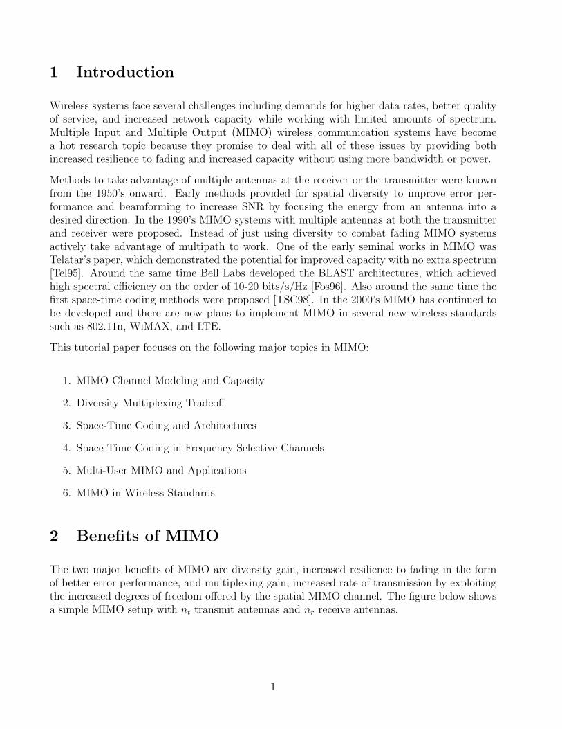
The two major benefits of MIMO are diversity gain, increased resilience to fading in the formof better error performance, and multiplexing gain, increased rate of transmission by exploitingthe increased degrees of freedom offered by the spatial MIMO channel. The figure below showsa simple MIMO setup with nt transmit antennas and nr receive antennas.
1

Figure 1: MIMO System Concept [Gold05]
2.1 Diversity
Diversity is an attempt to exploit redundancies in the way information is sent to achieve bet-ter error performance by cleverly using multiple copies of the same signal. Three fundamentaltypes of diversity are time, frequency, and antenna diversity. Time diversity involves averagingthe fading effects of the channel over time. The simplest example is the repetition code, whichtransmits the same symbol multiple times with the transmissions separated by more than the co-herence time of the channel. The receiver decodes each symbol independently and estimates thetransmitted symbol by majority rule. Frequency diversity exploits the variations in a frequencyselective channel. For example, orthogonal frequency division multiplexing(OFDM) can applymodulation order adaption to each subcarrier depending on the quality of a given subchannel.
Finally, there are several different types of antenna diversity. The most obvious type is to simplyuse multiple antennas. This type of antenna diversity is one of the main focuses of this paper.The second type of antenna diversity is to use multiple antennas with different polarizations.The third type of antenna diversity is to use multiple antennas with different non-overlappingbeam patterns.
It is generally of interest to quantify exactly how much diversity a given scheme provides. Thiscan be done through calculating either the average probability of error or the outage probability.Both of these expressions can generally be approximated as
SNR−L (1)
at high SNR. L is the diversity gain. This diversity gain can be more rigorously defined as
L = − limSNR→∞
log(Pe)
log(SNR)
This is just a formalization of the intuition above that replaces “at high SNR” with a limit. Forthe case of nt × nr narrowband MIMO the maximum possible diversity gain is ntnr, which isthe maximum number of independent copies of the same signal that the receiver sees.
2
2.1.1 Union Bound on Probability of Error
It can be difficult to calculate an exact expression for the probability of error for an arbitrarymodulation, so it is useful to calculate an upper bound on the probability of error. Consider anarbitrary constellation C containing M points. Write the constellation as
C = c1, c2, . . . , cM (2)
Let Pe be the probability of symbol error. Let Pe|cibe the probability of symbol error given
ci ∈ C was sent. Assuming all symbols are equally likely then
Pe =1
M
M∑m=1
Pe|cm (3)
The conditional probability of symbol of error can be expanded as
Pe|cm = P [cm is detected incorrectly | cm was transmitted]
=M∑l=1l 6=m
P [cm is estimated as cl | cm was transmitted]
Computing each of these probabilities is difficult and requires integration over a possibly com-plicated Voronoi region specific to each type of modulation. A simplifying approximation is thepairwise error probability(PEP) in which it is assumed for the purposes of calculation that onlycm and cl are in the constellation. This is denoted P [cm → cl]. For complex AWGN
P [cm → cl] = Q
√Ex
No
||cm − cl||22
(4)
PEP overestimates the probability of decoding cm as cl, so
Pe|cm ≤M∑l=1l 6=m
Q
√ P
No
||cm − cl||22
(5)
3
Then let d2min be the square of the minimum distance between points in the constellation C.
Then
Pe ≤ 1
M
M∑m=1
M∑l=1l 6=m
Q
√ P
No
||cm − cl||22
≤ 1
M
M∑m=1
M∑l=1l 6=m
Q
√ P
No
d2min
2
=1
M
M∑m=1
(M − 1)Q
√ P
No
d2min
2
= (M − 1)Q
√ P
No
d2min
2
(6)
The Chernoff bound on the Q-function is
Q(x) ≤ 1
2e−x2/2 (7)
So then the probability of error can be approximated as
Pe ≤M − 1
2e−
PNo
d2min4 (8)
This bound is very useful in calculating the diversity gain for simple multiple antenna systems.
2.1.2 Outage Probability
Formally the channel is in outage if the rate of transmission exceeds the channel capacity. Theoutage probability is the probability that this situation occurs: P [C < R]. From expressionsfor outage probability one can also find the diversity gain in a manner similar to the averageprobability of error method. For the typical Gaussian memoryless channel the channel capacityis C = B log2 (1 + SNR). Thus
P [B log2 (1 + SNR) < R] = P[SNR < 2R/B − 1
]Generally for other channels the outage condition reduces to the SNR being below a certainthreshold. Thus the diversity gain can generally be found from the probability:
P [SNR < γ]
4
2.2 Spatial Multiplexing
Besides providing diversity gain and improved error performance MIMO can also provide in-creased data rates and spectral efficiency through spatial multiplexing. To see how MIMOachieves this first consider QAM. The transmitted signal can be expressed as
xn(t) = an(t)cos(2πfct)− bn(t)sin(2πfct) (9)
assuming the appropriate normalizations have been made. This system has two real degrees offreedom (1 complex degree of freedom) because independent streams of bits could be transmittedon the cosine and sine terms. In practice, however, the two independent streams usually comefrom one original stream, which is demultiplexed by the symbol mapping operation into twostreams, which are placed on the cosine and sine terms.
Fundamentally MIMO provides increased rates in a similar way by providing even more degreesof freedom. The degrees of freedom in MIMO come from the multiple antennas transmittingindependent streams. In the 4 × 4 MIMO case, for example, each transmit antenna can sendan independent stream, which will be received by all four antennas simultaneously, so thereare four degrees of freedom. The maximum possible complex degrees of freedom for MIMO isminnt, nr.
3 Basic Schemes for Multiple Antennas
Now consider a few basic multiple antennas schemes that can provide diversity. The majorassumptions underlying these schemes are whether the receiver has channel information(CSIR)or the transmitter has channel information(CSIT). CSIR is a pretty common assumption andcan be achieved through several estimation methods. CSIT is trickier to achieve as the receivermust estimate the channel and feed the estimate back to the transmitter through a feedbackchannel in FDD or the transmitter must assume that it sees the same channel as the receiver inTDD. Feedback entails a cost in terms of lost capacity and bandwidth.
3.1 Channel Models
The channel model for these basic MIMO schemes is a simple extension of the scalar Rayleighchannel. The channels are now modeled as complex Gaussian vectors with CN (0, I) distribution.This channel model is justified in terms of physical propagation models in the next section.
5
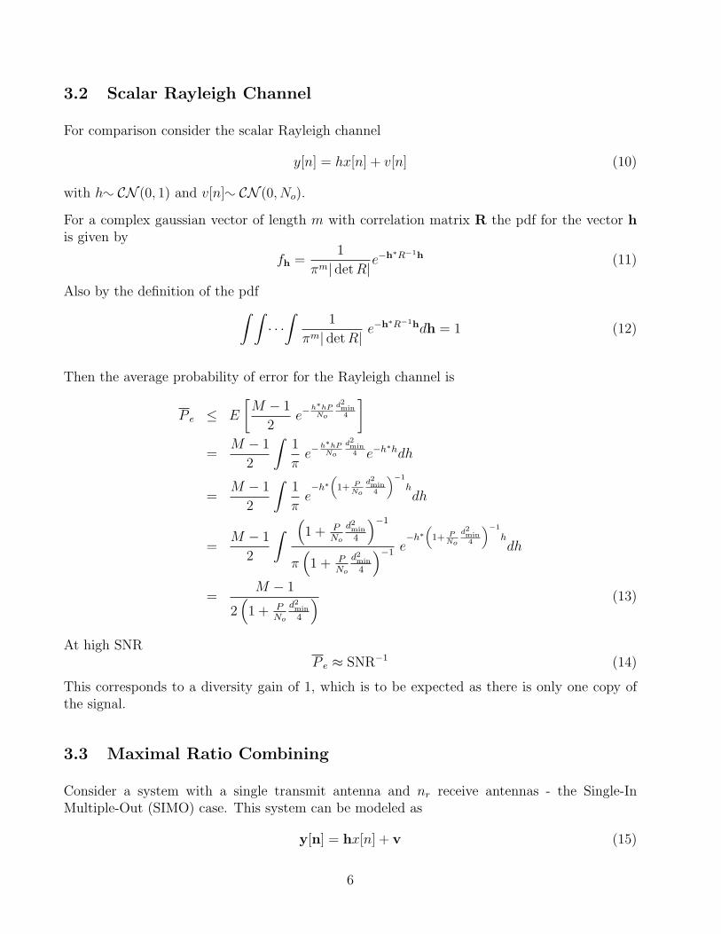
3.2 Scalar Rayleigh Channel
For comparison consider the scalar Rayleigh channel
y[n] = hx[n] + v[n] (10)
with h: CN (0, 1) and v[n]: CN (0, No).
For a complex gaussian vector of length m with correlation matrix R the pdf for the vector his given by
fh =1
πm| det R|e−h∗R−1h (11)
Also by the definition of the pdf∫ ∫· · ·∫
1
πm| det R|e−h∗R−1hdh = 1 (12)
Then the average probability of error for the Rayleigh channel is
P e ≤ E
[M − 1
2e−
h∗hPNo
d2min4
]=
M − 1
2
∫1
πe−
h∗hPNo
d2min4 e−h∗hdh
=M − 1
2
∫1
πe−h∗
„1+ P
No
d2min4
«−1
hdh
=M − 1
2
∫ (1 + P
No
d2min
4
)−1
π(1 + P
No
d2min
4
)−1 e−h∗
„1+ P
No
d2min4
«−1
hdh
=M − 1
2(1 + P
No
d2min
4
) (13)
At high SNRP e ≈ SNR−1 (14)
This corresponds to a diversity gain of 1, which is to be expected as there is only one copy ofthe signal.
3.3 Maximal Ratio Combining
Consider a system with a single transmit antenna and nr receive antennas - the Single-InMultiple-Out (SIMO) case. This system can be modeled as
y[n] = hx[n] + v (15)
6
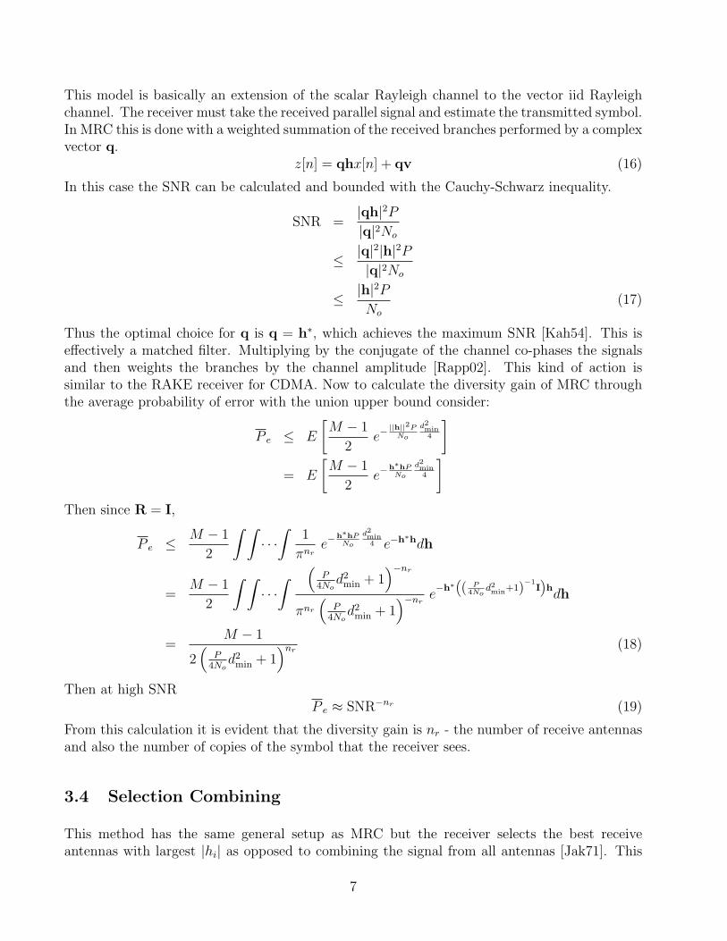
This model is basically an extension of the scalar Rayleigh channel to the vector iid Rayleighchannel. The receiver must take the received parallel signal and estimate the transmitted symbol.In MRC this is done with a weighted summation of the received branches performed by a complexvector q.
z[n] = qhx[n] + qv (16)
In this case the SNR can be calculated and bounded with the Cauchy-Schwarz inequality.
SNR =|qh|2P|q|2No
≤ |q|2|h|2P|q|2No
≤ |h|2PNo
(17)
Thus the optimal choice for q is q = h∗, which achieves the maximum SNR [Kah54]. This iseffectively a matched filter. Multiplying by the conjugate of the channel co-phases the signalsand then weights the branches by the channel amplitude [Rapp02]. This kind of action issimilar to the RAKE receiver for CDMA. Now to calculate the diversity gain of MRC throughthe average probability of error with the union upper bound consider:
P e ≤ E
[M − 1
2e−
||h||2PNo
d2min4
]= E
[M − 1
2e−
h∗hPNo
d2min4
]Then since R = I,
P e ≤ M − 1
2
∫ ∫· · ·∫
1
πnre−
h∗hPNo
d2min4 e−h∗hdh
=M − 1
2
∫ ∫· · ·∫ (
P4No
d2min + 1
)−nr
πnr
(P
4Nod2
min + 1)−nr
e−h∗
“( P
4Nod2min+1)
−1I”hdh
=M − 1
2(
P4No
d2min + 1
)nr(18)
Then at high SNRP e ≈ SNR−nr (19)
From this calculation it is evident that the diversity gain is nr - the number of receive antennasand also the number of copies of the symbol that the receiver sees.
3.4 Selection Combining
This method has the same general setup as MRC but the receiver selects the best receiveantennas with largest |hi| as opposed to combining the signal from all antennas [Jak71]. This
7
method can achieve the same diversity gain as MRC - nr. Assuming each branch has amplitudesk, then as outlined in [SA00]
P [maxs1, s2, . . . , snr < S] =(1− e−S2
)nr
(20)
So the pdf of smax is given by
psmax(S) = nr2Se−S2(1− e−S2
)nr−1
(21)
Then the average received SNR is
SNR = Pnr∑i=1
1
i(22)
It is obvious from this equation that increasing the number of receive antennas provides adiminishing return. Most of the gain comes from going from one receive antenna to two andthree receive antennas.
3.5 Equal Gain Combining
The branches from each antenna are first co-phased to cancel out the effects of the channel andthen they are simply added together to produce the output. If the channel tap hi = αie
jθi , thenthe co-phasing operation is simply a multiplication of each branch by e−jθi . Equal gain combiningproduces performance similar to MRC and achieves the full diversity gain as demonstrated in[Yac93], but with a 1-3 dB penalty depending on the exact setup and number of antennas.
3.6 Transmit Maximal Ratio Combining
We have considered the SIMO case and now it is time to consider the Multiple-In Single-Out(MISO) case with nt transmit antennas. With multiple transmit antennas it is important tokeep the total transmit power P constant to allow a fair comparison to the cases with only onetransmit antenna. The question now is if any diversity gain can be achieved and if so how? Afirst attempt to achieve diversity gain with multiple transmit antennas is to simply transmit thesame symbol on each branch. However, this method does not achieve any diversity gain. To getan intuitive explanation for this one can consider the effective channel that the receiver sees tobe
h1 + h2 + · · ·+ hnt√nt
: CN (0, 1) (23)
The 1√nt
normalizes the transmit power. This effective channel behaves like a scalar Rayleigh
channel, which provides no diversity gain beyond the scalar Rayleigh channel.
An approach that does work is Transmit Maximal Ratio Combining (TMRC), which requiresCSIT and is a close analog of MRC. The system can be modeled as
y = hx + v (24)
8
A weighting vector q sends a weighted version of the current symbol x to each antenna. So then
y = hqx + v (25)
Then by a derivation similar to MRC it can be shown that the optimal choice for q is q = h∗
[God97]. The diversity gain for this scheme is nt.
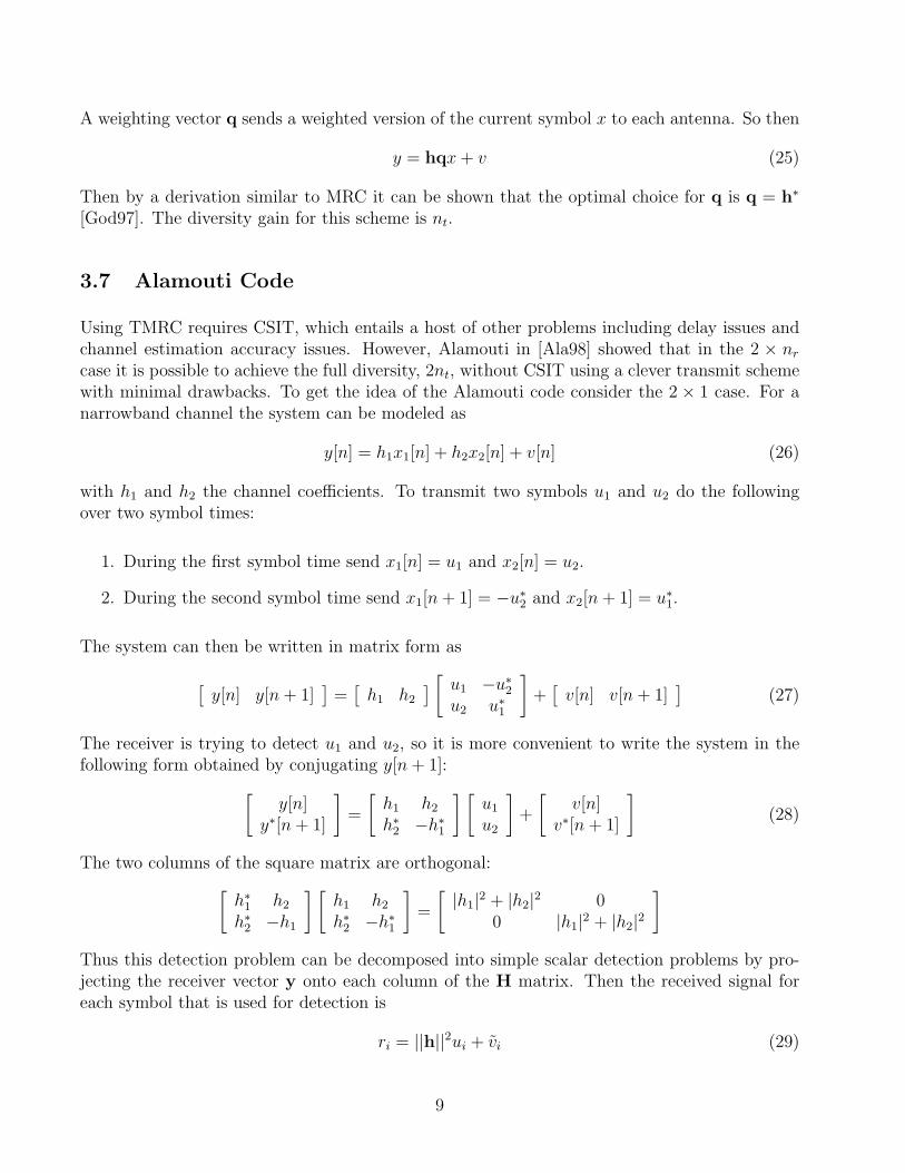
3.7 Alamouti Code
Using TMRC requires CSIT, which entails a host of other problems including delay issues andchannel estimation accuracy issues. However, Alamouti in [Ala98] showed that in the 2 × nr
case it is possible to achieve the full diversity, 2nt, without CSIT using a clever transmit schemewith minimal drawbacks. To get the idea of the Alamouti code consider the 2 × 1 case. For anarrowband channel the system can be modeled as
y[n] = h1x1[n] + h2x2[n] + v[n] (26)
with h1 and h2 the channel coefficients. To transmit two symbols u1 and u2 do the followingover two symbol times:
1. During the first symbol time send x1[n] = u1 and x2[n] = u2.
2. During the second symbol time send x1[n + 1] = −u∗2 and x2[n + 1] = u∗1.
The system can then be written in matrix form as
[y[n] y[n + 1]
]=[
h1 h2
] [ u1 −u∗2u2 u∗1
]+[
v[n] v[n + 1]]
(27)
The receiver is trying to detect u1 and u2, so it is more convenient to write the system in thefollowing form obtained by conjugating y[n + 1]:[
y[n]y∗[n + 1]
]=
[h1 h2
h∗2 −h∗1
] [u1
u2
]+
[v[n]
v∗[n + 1]
](28)
The two columns of the square matrix are orthogonal:[h∗1 h2
h∗2 −h1
] [h1 h2
h∗2 −h∗1
]=
[|h1|2 + |h2|2 0
0 |h1|2 + |h2|2]
Thus this detection problem can be decomposed into simple scalar detection problems by pro-jecting the receiver vector y onto each column of the H matrix. Then the received signal foreach symbol that is used for detection is
ri = ||h||2ui + vi (29)
9

with vi: CN (0, No). In detection the vector channel is decomposed into a scalar Rayleighchannel for each symbol. The Alamouti code is representative of a larger class of codes callorthogonal space-time block codes (O-STBCs) that also have easy detection due to orthogonality.
It can be shown that the diversity gain is 2. Since each symbol is transmitted twice, thetransmit power of each antenna must be reduced by 3 dB compared to the single antenna caseto normalize the total power. This power loss hurts detection but no so much as to make theAlamouti code useless. In fact, there are some advantages to using antennas transmitting withlower power. At lower power it is easier to find cheap amplifiers that can operate in the linearregion. Also the Alamouti code transmits two symbols over two symbol periods, so its effectiverate of transmission is the same as the original symbol rate.
Finally, the Alamouti code can be extended to the full 2×nr case by using the same transmissionscheme as the 2× 1 case and MRC. This method provides the full 2nr diversity gain.
Figure 2: Comparison of Alamouti and MRC Error Performance [OC06]
4 MIMO Channel Modeling and Capacity
In this section we will consider several MIMO channels and the physical meaning behind thesechannels. Of particular interest is how the structure of a MIMO channel suggests the gains ofMIMO. For all MIMO channels we will assume the rate of transmission is high enough that thechannel will be slow fading, which is a reasonable assumption in any modern high speed wirelesssystem.
10
4.1 Narrowband MIMO Channel
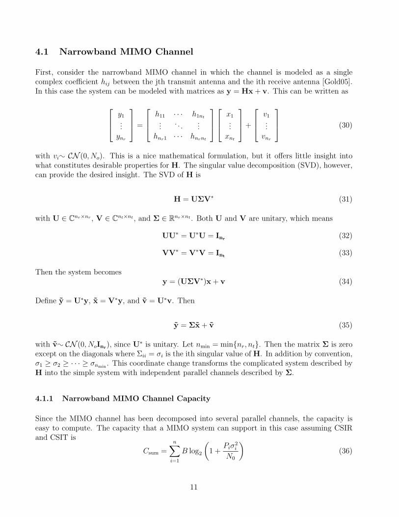
First, consider the narrowband MIMO channel in which the channel is modeled as a singlecomplex coefficient hij between the jth transmit antenna and the ith receive antenna [Gold05].In this case the system can be modeled with matrices as y = Hx + v. This can be written as
y1...
ynr
=
h11 · · · h1nt
.... . .
...hnr1 · · · hnrnt
x1
...xnt
+
v1...
vnr
(30)
with vi: CN (0, No). This is a nice mathematical formulation, but it offers little insight intowhat constitutes desirable properties for H. The singular value decomposition (SVD), however,can provide the desired insight. The SVD of H is
H = UΣV∗ (31)
with U ∈ Cnr×nr , V ∈ Cnt×nt , and Σ ∈ Rnr×nt . Both U and V are unitary, which means
UU∗ = U∗U = Inr (32)
VV∗ = V∗V = Int (33)
Then the system becomesy = (UΣV∗)x + v (34)
Define y = U∗y, x = V∗y, and v = U∗v. Then
y = Σx + v (35)
with v: CN (0, NoInr), since U∗ is unitary. Let nmin = minnr, nt. Then the matrix Σ is zeroexcept on the diagonals where Σii = σi is the ith singular value of H. In addition by convention,σ1 ≥ σ2 ≥ · · · ≥ σnmin
. This coordinate change transforms the complicated system described byH into the simple system with independent parallel channels described by Σ.
4.1.1 Narrowband MIMO Channel Capacity
Since the MIMO channel has been decomposed into several parallel channels, the capacity iseasy to compute. The capacity that a MIMO system can support in this case assuming CSIRand CSIT is
Csum =n∑
i=1
B log2
(1 +
Piσ2i
N0
)(36)
11
as demonstrated in [CT91, CKT98, Tel95]. The power allocation Pi can be chosen by tryingto maximize Csum subject to the constraint
∑nmin
i=1 Pi = P . Lagrange multipliers can be used inthis case to compute the optimal power allocation.
∂
∂Pi
(nmin∑i=1
B log2
(1 +
Piσ2i
N0
))= λ
∂
∂Pi
(nmin∑i=1
Pi
)Bσ2
i
(Piσ2i + No) log(2)
= λ
Pi =B
λ log(2)− No
σ2i
(37)
with λ chosen such that∑nmin
i=1 Pi = P . This power allocation method is known as the waterfillingpower allocation. The term B
λ log(2)represents the surface of the water and the No
σ2i
term represents
the depth of the water for any singular value.
4.1.2 Rank and Condition Number
Let k be the number of nonzero singular values of H, which is also the rank of H. At high SNRthe waterfilling allocation is close to the uniform power allocation, so
C ≈k∑
i=1
B log2
(1 +
Pσ2i
kNo
)≈ k log2(SNR) +
k∑i=1
log2
(σ2
i
k
)(38)
k is thus the parameter that controls the number of spatial degrees of freedom and hence thenumber of independent streams that can be multiplexed [TV05]. So obviously we want k aslarge as possible, which is nmin at most in the case that H has full rank. That the channelcapacity increases linearly in nmin at high SNR is one of the most attractive features of MIMO.
Jensen’s inequality can give more information about behavior of the capacity with respect toH.
k∑i=1
B log2
(1 +
Pσ2i
kNo
)≤ B log2
(1 +
P
kNo
k∑i=1
σ2i
)(39)
This suggests that the quantity∑k
i=1 σ2i should be maximized. This is achieved precisely when
all the singular values are roughly equal. In other words σmax
σmin≈ 1. In matrix theory this quantity
is the condition number, κ(H), and a matrix with κ(H) ≈ 1 is said to be well-conditioned. ThusH should be well conditioned to ensure a large capacity.
4.2 Physical Modeling of MIMO Channels
The major goal of this section is to see how MIMO’s ability to spatially multiplex depends onthe actual propagation environment. Also, this section will examine what must be true of thepropagation to ensure that the rank and condition number criteria are satisfied. All antennaarrays in this section are assumed to be linear and uniformly spaced.
12
4.2.1 LOS SIMO and MISO Channel
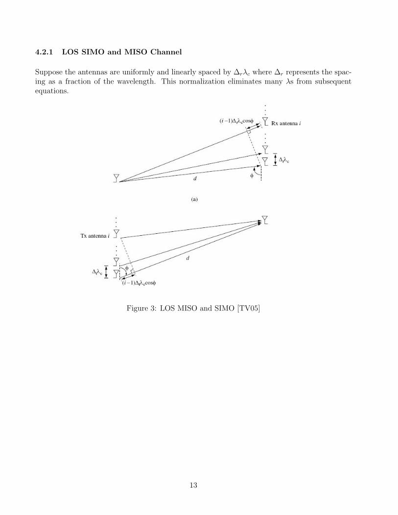
Suppose the antennas are uniformly and linearly spaced by ∆rλc where ∆r represents the spac-ing as a fraction of the wavelength. This normalization eliminates many λs from subsequentequations.
Figure 3: LOS MISO and SIMO [TV05]
13
The impulse responses between the transmit antenna and each receive antenna are
hi(τ) = aδ(τ − di/c) (40)
a models the path loss of the propagating wave and the di/c term models the time it takes for apropagating EM wave to reach the ith receive antenna [SMB01]. At baseband the channel gainis given by
hi = a e−j2πdi/λc (41)
So then the channel can be modeled with AWGN as
y = hx + n (42)
with h = [h1, h2, . . . , hnr ] and w: CN (0, NoInr). For large d
di ≈ d + (i− 1)∆rλc cos(φ) (43)
Define Ω = cos(φ). Define the following quantity from [Fle00]:
ar(Ω) =1
√nr
1
e−j2π∆rΩ
...e−j2π(nr−1)∆rΩ
(44)
Then the following important identity holds:
a∗r(Ω)ar(Ω) =1
nr
[1 ej2π∆rΩ · · · ej2π(nr−1)∆rΩ
]
1e−j2π∆rΩ
...e−j2π(nr−1)∆rΩ
=
1
nr
((1) (1) +
(ej2π∆rΩ
) (e−j2π∆rΩ
)+ · · ·+
(ej2π(nr−1)∆rΩ
) (e−j2π(nr−1)∆rΩ
))a∗r(Ω)ar(Ω) = 1 (45)
Then the channel h can be written as
h = a e−j2πd/λc√
nrar(Ω) (46)
as demonstrated in [SMB01]. The channel capacity is
C = B log2
(1 +
P ||h||2
No
)= B log2
(1 +
Pa2nr
No
)(47)
as given in [TV05]. Thus there is a power gain and increased capacity potentially but no degreeof freedom gain and so no spatial multiplexing is possible.
The MISO case is similar and involves the use of
at(Ω) =1√
nt
1
e−j2π∆tΩ
...e−j2π(nt−1)∆tΩ
(48)
14
4.2.2 LOS MIMO
Similarly to the SIMO case the baseband equivalent channel is
hij = ae−j2πdij/λc (49)
If d is large thendij ≈ d + (i− 1)∆rλc cos(φr)− (j − 1)∆tλc cos(φt) (50)
as shown in [TV05]. Define Ωr = cos(φr) and Ωt = cos(φt). Then the channel matrix is givenby
H = a√
ntnre−j2πd/λc ar(Ωr)a
∗t(Ωt) (51)
In this case H has rank 1 and the only singular value is a√
ntnr. Then the capacity is
C = B log2
(1 +
Pa2ntnr
No
)(52)
This is the same result as the SIMO/MISO case: no degree of freedom gain.
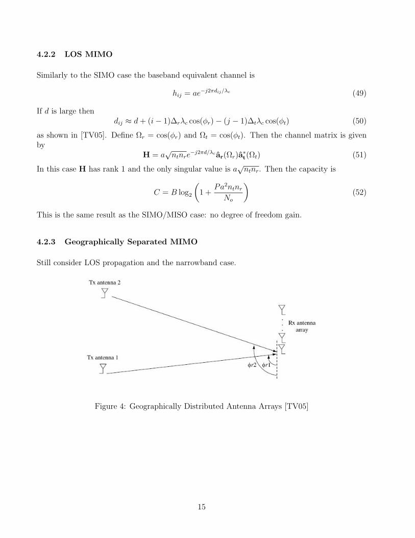
4.2.3 Geographically Separated MIMO
Still consider LOS propagation and the narrowband case.
Figure 4: Geographically Distributed Antenna Arrays [TV05]
15
Then the channel between the kth transmit antenna and all the receive antennas is
hk = ak
√nre
−j2πdk/λc ar(Ωrk) (53)
with dk the distance between the kth transmit antenna and the first receive antenna [PNG03,Her04]. ar(Ω) is periodic with period 1/∆r. Also, the function ar(Ω) doesn’t take on the samevalue twice in one period, so ar(Ωr1) and ar(Ωr2) are linearly independent as long as Ωr1−Ωr2 isnot an integer multiple of 1/∆r. In the 2× nr case as long as the two angles are not a multipleof 1/∆r the two rows of H are linearly independent and thus H has full rank. Thus in thiscase spatial multiplexing is possible. Now what remains to be considered is whether H is well-conditioned. To determine this consider the angle θ between the two columns of H associatedwith the two transmit antennas. This angle satisfies
| cos(θ)| = |a∗r(Ωr1)ar(Ωr2)| (54)
=
∣∣∣∣ sin(πLrΩr)
nr sin(πLrΩr/nr)
∣∣∣∣ (55)
with Lr = nr∆r. Then the two singular values are
λ1 =√
a2nr(1 + | cos θ|), λ2 =√
a2nr(1− | cos θ|) (56)
Thus
κ(H) =
√1 + | cos θ|1− | cos θ|
(57)
Thus the matrix is ill conditioned whenever | cos(θ)| ≈ 1, which occurs when
|Ωr −m
∆r
| <<1
Lr
(58)
for some integer m. So basically when the difference between two directional cosines of twoangular paths are within 1
Lrthe receiver can’t distinguish between the two paths. This is similar
to the case in frequency selective channels in which the bandwidth of the system controls whichmultipath delays can be resolved.
4.2.4 Two-Ray MIMO
Consider the full MIMO case with antenna arrays at both the transmitter and receiver. Let d(i)
be the distance between transmit antenna 1 and receiver antenna 1 along path i.
Definea′
i = ai
√ntnr e−j2πdi/λc (59)
Then the channel matrix can be expressed as
H = a′
1ar(Ωr1)a∗t(Ωt1) + a
′
2ar(Ωr2)a∗t(Ωt2) (60)
16

Figure 5: Two-Ray MIMO [TV05]
as in [PNG03, Her04]. This expression for the channel can be put in matrix form as
H =[
a′1ar(Ωr1) a
′2ar(Ωr2)
] [ a∗t(Ωt1)a∗t(Ωt2)
](61)
To ensure H has rank 2 the following two conditions must hold:
Ωt1 6= Ωt2 mod1
∆r
(62)
Ωr1 6= Ωr2 mod1
∆r
(63)
H has rank 2 so spatial multiplexing is possible. To ensure that H is well conditioned it isnecessary that Ωr2−Ωr1 ≥ 1
Lrand Ωt2−Ωt1 ≥ 1
Ltthat is to say there must be sufficient angular
separation at the transmitter and receiver to ensure that the paths can be resolved.
4.3 Statistical Modeling of MIMO Channels
In the case of a frequency selective channel the channel can be modeled as an FIR filter withtaps h[n]. In this case not all individual multipath components can be resolved but only mul-tipath components that differ in delay by a sufficient amount related to the system bandwidth.In modeling a MIMO channel the interest is not in time resolution of multipath but angularresolution at the transmitter and receiver [Par00].
Suppose the transmit and receive antenna lengths are Lt and Lr. Paths that have Ωs that differby less than 1
Ltat the transmitter or 1
Lrat the receiver can not be resolved. The term hij is
the aggregation of all paths of angular spacing 1Lt
about jLt
and angular spacing 1Lr
about iLr
.If there are an arbitrary number of paths then the channel is given by
H =∑
i
a′
iar(Ωri) a∗t(Ωti) (64)
The received and transmitted signals can always be expressed in terms of the follow pair of
17

basis:
Sr =
ar(0), ar(
1
Lr
), . . . , ar(nr − 1
Lr
)
(65)
St =
at(0), at(
1
Lt
), . . . , at(nt − 1
Lt
)
(66)
which represent the angular bins.
Figure 6: Angular Domain MIMO [TV05]
Each basis can be used to represent transmitted and received signals in the angular domain interms of the directional cosine Ω. Let Ut be the nt × nt matrix with columns from St. If x is avector transmitted by the antennas, then in the angular domain xa are related by
x = Utxa, xa = U∗
tx (67)
By examining the matrix Ut it can be seen that xa is the IDFT of x. Then define ya = U∗ry.
In this coordinate system
ya = U∗rHUtx
a + va
= Haxa + va (68)
Each element haij can be reasonably modeled as independent circularly symmetric complex Gaus-
sian r.v. like the Rayleigh channel. The validity of this assumption rests on two key factors
18
• Amount of scattering and reflection in the multipath environment - this model needsseveral multipath components in each angular bin
• The lengths of Lt and Lr - Short antenna arrays lump many multipath components intothe same angular bin. A longer antenna array results in better angular resolution of pathsand more non-zero entries in Ha.
Since Ut and Ur are unitary andH = UrH
aU∗t (69)
H has the same iid Gaussian distribution [CT91]. Thus in the narrowband case the MIMOchannel is basically an extension of the scalar Rayleigh channel where each coefficient of thechannel matrix is a complex Gaussian random variable. In addition, results from random matrixtheory show that H with this distribution has full rank with probability 1. Thus the channel inthis model can support spatial multiplexing.
If there is a strong line-of-sight component, then the fading is not Rayleigh but Ricean.
Antenna Spacing The assumption that the coefficients of H are independent or at leastuncorrelated depends heavily on the antenna spacing. As a rule of thumb antenna spacing ofat least λ
2is desirable and results in uncorrelated coefficients [FG98]. As the antenna spacing
increases there is still a diversity gain but it is not quite as large as if the antennas werespaced further. As the antenna spacing decreases towards λ
4the channel coefficients become
strongly correlated. The exact amount of correlation depends on the angular spread of theantennas. For antennas with small angular spread at separations on the order of λ
4or smaller
the coefficients are highly correlated. Since the coefficients are highly correlated the receiverdoes not see as many independent copies of the transmitted signal, so the achievable diversitygain is reduced. In practice the channel coefficients are never completely uncorrelated butas a simplifying assumption to make analysis tractable we assume they are uncorrelated andindependent.
4.3.1 Frequency Selective MIMO Channel
The extension of the preceding flat MIMO channel model to the frequency selective MIMOchannel model is fairly straightforward. The channel in this case can be modeled as
y[n] =N∑
l=1
Hlx[n− l] + v[n] (70)
as in [TV05]. In this model the channel between any two pairs of antennas is modeled as ascalar frequency selective channel in which the output is a convolution of the input and thechannel taps. The justification for this model is a straightforward extension of the angularmodel outlined in the previous sections.
19

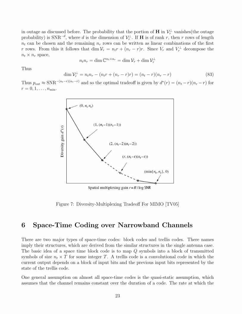
5 Diversity-Multiplexing Tradeoff
A MIMO system can transmit one symbol on all the transmit antennas and use the right pro-cessing to obtain the full diversity gain ntnr. On the other hand a MIMO system can transmitnmin independent streams to provide the maximum possible rate with the minimum error protec-tion. The diversity-multiplexing tradeoff involves investigating what happens between these twoextremes and in particular what constitutes the optimal tradeoff. In particular, transmitting ata given rate what is the maximum possible diversity gain. This kind of analysis leads to a curverelating the transmit rate and the optimal diversity gain. Of great interest is whether a givenspace-time code or modulation can achieve this frontier and thus be optimal.
This tradeoff curve is difficult to compute, but some methods have been proposed to simplifythe study of this tradeoff. Tse and Zheng proposed in [ZT03] studying this tradeoff by makingassumptions on the possible rates of transmission and letting the SNR approach infinity. Athigh SNR the MIMO capacity is
C ≈ nmin log2(SNR) (71)
for a channel with full rank. Tse and Zheng assumed that only rates R = r log(SNR) arepossible with r = 0, 1, . . . , nmin. The optimal diversity gain, d∗(r), is the exponent in the outageprobability, so
pout ≈ SNR−d∗(r) (72)
Thus it makes sense to define
d∗(r) = − limSNR→∞
log pout(r log SNR)
log SNR(73)
Alternatively d∗(r) can be defined in terms of the probability of error
d∗(r) = − limSNR→∞
log Pe(r log SNR)
log SNR(74)
Before tackling the full MIMO channel it is useful to consider the diversity-multiplexing tradeoffin scalar and SIMO/MISO channels.
5.1 Scalar Rayleigh Channel
The scalar channel is in outage if the capacity it supports falls below the rate of transmission.So pout is given by
pout = P[log(1 + |h|2SNR
)< r log SNR
]= P
[|h|2 <
SNRr − 1
SNR
]|h|2 is chi-squared distributed. For sufficiently large ε, P [|h|2 < ε] ≈ ε. Thus the outageprobability is approximately
pout ≈1
SNR1−r (75)
Thus d∗(r) = 1− r is the optimal tradeoff.
20

5.1.1 QAM over the Scalar Rayleigh Channel
It can be demonstrated that for QAM that Pe ≈ 2R
SNR. Then
d(r) = − limSNR→∞
log Pe
log SNR
= − limSNR→∞
log(2r log SNR/SNR
)log SNR
= − limSNR→∞
r log SNR− log SNR
log SNR
= 1− r (76)
Thus QAM achieves the optimal diversity-multiplexing tradeoff of the scalar Rayleigh channel.
5.2 MISO Rayleigh Channel
In this case the system can be modeled as
y[n] = hx[n] + w[n] (77)
Taking the rate R = r log SNR as usual the outage probability is
pout = P
[log
(1 + ||h||2 SNR
nt
)< r log SNR
](78)
||h||2 is χ2n distributed so the approximation P [||h||2 < ε] ≈ εnt can be used. Then the outageprobability is roughly
pout ≈ SNR−nt(1−r) (79)
So it is apparent that the optimal tradeoff d∗(r) = nt(1− r).
The Alamouti code effectively decomposes the MISO channel into parallel Rayleigh channel. Itcan be easily demonstrated that the optimal tradeoff curve for this parallel Rayleigh channel isd∗(r) = 2(1 − r). So if QAM is used on each of the scalar channels along with the Alamouticode, then the resulting system is tradeoff optimal for the MISO channel.
5.3 MIMO Rayleigh Channel
The outage probability is given by
pout = minKx:Tr[Kx]≤SNR
P [log det (Inr + HKxH∗) < r log SNR] (80)
The matrix Kx is the covariance matrix of the input and basically represents a power allocation.The power allocation at the transmitter directly affects the SNR at the receiver. This scheme
21
makes a specific assumption about the rate R at a given SNR, so the input covariance matrixmust be chosen not to exceed the limit. The worst covariance matrix Kx is approximately 1
ntInr ,
so
pout = P
[log det
(Inr +
SNR
nt
HH∗)
< r log SNR
](81)
This outage probability can be written in terms of the singular values of H as
pout = P
[nmin∑i=1
log
(1 +
SNR
nt
σ2i
)< r log SNR
](82)
There are no neat approximations to evaluate this outage probability but there is a neat geo-metric argument to evaluate the outage probability [TV05, ZT03]. First consider r close to 0.Outage occurs when H is close to 0. Close can be evaluated in terms of the Froebnius norm
||H− 0||F = ||H||F
=
nmin∑i=1
σ2i
=∑i,j
|hij|2
Thus the magnitude of each channel coefficient |hij| must be close to 0 for the channel to be inoutage.
Now if r is an integer greater than 0 the situation becomes considerably more complicated, sincethere are more ways to choose bad λi to put the channel in outage. The situation seems hopelessbut it has been shown by Tse and Zheng that although there are many ways for the channel tobe in outage the most common way is for r eigenchannels to be good and the remained to bebad. In this case H has rank r and H is in the space Vr of rank r matrices in the space Cnt×nr .So the question of whether H puts the channel in outage is the question of whether H is closeto Vr in the appropriate sense.
This question is tractable but also a little tricky, since Vr is not a linear space. The followingparagraph is very technical but the fundamental result is simple: Vr can be considered to be alinear space in a sufficiently small neighborhood. To see that Vr is not linear consider that if Vr
were a linear space, then 0 ∈ Vr. But clearly 0 has rank 0, so 0 /∈ Vr. Thus Vr is not a linearsubspace of Cnt×nr . However, although it turns out that Vr may not be a linear subspace, it is amanifold embedded in Cnt×nr . A manifold is a space with the property that small neighborhoodsof a point look like linear subspaces of Rk or Ck. For example, the surface of Earth is a manifoldsince a small neighborhood looks like a portion of R2 even though the overall space is clearlynot linear. The question of interest is what happens when H is close to Vr, so it is sufficient toconsider a small neighborhood N of a point of Vr containing H. N looks like a linear subspaceof Cnt×nr . For the remainder of this argument restrict our consideration to N .
Since Vr can be considered locally linear, the notion of orthogonality can be used. Then H canbe decomposed into a portion in Vr and a portion in the space V⊥r , which is orthogonal to Vr. Ifthe portion of H in V⊥r vanishes, then H is basically in Vr, H has rank r, and so the channel is
22
in outage as discussed before. The probability that the portion of H in V⊥r vanishes(the outageprobability) is SNR−d, where d is the dimension of V⊥r . If H is of rank r, then r rows of lengthnt can be chosen and the remaining nr rows can be written as linear combinations of the firstr rows. From this it follows that dimVr = ntr + (nr − r)r. Since Vr and V ⊥
r decompose thent × nr space,
ntnr = dim Cnt×nr = dimVr + dimV⊥rThus
dimV⊥r = ntnr − (ntr + (nr − r)r) = (nt − r)(nr − r) (83)
Thus pout ≈ SNR−(nt−r)(nr−r) and so the optimal tradeoff is given by d∗(r) = (nt− r)(nr − r) forr = 0, 1, . . . , nmin.
Figure 7: Diversity-Multiplexing Tradeoff For MIMO [TV05]
6 Space-Time Coding over Narrowband Channels
There are two major types of space-time codes: block codes and trellis codes. There namesimply their structures, which are derived from the similar structures in the single antenna case.The basic idea of a space time block code is to map Q symbols into a block of transmittedsymbols of size nt × T for some integer T . A trellis code is a convolutional code in which thecurrent output depends on a block of input bits and the previous input bits represented by thestate of the trellis code.
One general assumption on almost all space-time codes is the quasi-static assumption, whichassumes that the channel remains constant over the duration of a code. The rate at which the
23

Figure 8: Space-Time Encoder Structure
channel changes is related to the coherence time, which is in turn related to the Doppler spread.The system must be designed to ensure that the duration of a codeword is less than the coherencetime. The channel can change between codewords, but not in the middle of codewords.
6.1 Error Motivated Design
It is important and interesting to find conditions that will guarantee a good error performancefor a space-time code. One approach to finding these conditions for the slow fading MIMOchannel is to consider what factors affect ML decoding of the codewords. The optimal way todetect a codeword is with ML detection is given by
C = arg minC∈C
||Y −HC||2 (84)
The operation of this detector is limited mainly by the closest pair of codewords. If two code-words are close together, then noise can lead to incorrect estimation of a codeword as anothercodeword. Then the error probability of interest is the paired error probability(PEP) that acodeword C is incorrectly decoded as E. Conditioning on the channel matrix H the PEP is[Pro01]
P [C → E|H] = Q
√√√√SNR
2
T∑k=0
||H(ck − ek)||2F
(85)
Averaging over all channel realization gives the average PEP: P [C → E]. In a way similar tothe diversity-multiplexing tradeoff the diversity gain, dg can be defined in terms of the PEP as
dg = − limSNR→∞
log P [C → E]
log SNR(86)
Generally at high SNR the PEP is of the form (c × SNR)−dg . The quantity c improves per-formance and is called the coding gain. A good space-time code should then achieve a highdiversity gain and a high coding gain.
The relevant question now is how to achieve diversity and coding gains. The covariance of two
24
codewords C and E is the matrix E = (E−C)(E−C)∗. Then the PEP is given by [SA00, Sim01],
P [C → E] =1
π
∫ π/2
0
[det
(Int +
SNR
4 sin2 βE
)]−nr
dβ
=1
π
∫ π/2
0
rank(E)∏i=1
(1 +
SNR
4 sin2 βλi
)−nr
dβ
≤rank(E)∏
i=1
(1 +
SNR
4λi
)−nr
with the second expansion due to expressing the determinants in terms of the eigenvalues λi(E)and the last expansion valid at high SNR. This expression can be further bounded to yield
P [C → E] ≤(
SNR
4
)−nrrank(E)rank(E)∏
i=1
λi
−nr
(87)
Thus the diversity gain is nrrank(E) and the coding gain is∏rank(E)
i=1 λi. Given these two gainsthere are two criterion for a good space-time code at high SNR are as follows [TSC98]:
• Rank Criterion - Maximize the minimum rank of the codeword difference matrix toachieve a good diversity gain always:
max
minC,E∈CC 6=E
rank(E)
(88)
• Determinant Criterion - Maximize the product of the nonzero eigenvalues to achievecoding gain
dλ = minC,E∈CC 6=E
rank(E)∏i=1
λi
(89)
In the case where the codeword matrix always has full rank this becomes maximize
dλ = minC,E∈CC 6=E
det E (90)
These criteria guarantee good codes at high SNR.
6.2 Space-Time Block Codes
A space-time block code(STBC) maps a block of Q input symbols into a block of symbols ofsize nt×T to be transmitted on the antennas. A quantity of interest is the effective symbol rateof the code:
rs =Q
T(91)
25
For rs = 1 the system effectively transmits one symbol per symbol period. For rs < 1 the systemon average transmits less than one symbol per symbol period. Codes with rs < 1 effectivelyreduce the rate of transmission.
6.2.1 Linear STBCs
There are many different classes of space-time block codes, but one of the most common is thelinear block code. The codeword of the linear block matrix can be expressed as a linear functionof complex nt × T basis matrices φq and input symbols c1, c2, . . . , cQ as follows [HH01]:
C =
Q∑q=1
φq<cq+ φq+C=cq (92)
It may seem a little odd to break up the real and imaginary components of the symbols, but theadvantage of this approach is that conjugation of symbols can be used in linear STBCs. Thefollowing example with the Alamouti code shows that this is possible.
Example: Alamouti code The two complex symbols c1 and c2 are mapped into the followingmatrix, which represents the Alamouti code:[
c1 −c∗2c2 c∗1
](93)
Then the code can be represented with basis matrices as:
φ1 =
[1 00 1
]φ2 =
[0 −11 0
]φ3 =
[1 00 −1
]φ4 =
[0 11 0
](94)
Code Design Criteria for Linear STBCs As we saw in the previous section minimizingthe worst PEP is a good strategy to develop a good space-time code. In the case of linearSTBCs if the basis matrices are unitary meaning φ∗φ = Int if T ≤ nt (Tall matrix) or φφ∗ = IT
if T ≥ nt (Wide matrix), then the PEP condition is
φqφ∗p + φpφ
∗q = 0 q 6= p (Wide) (95)
φ∗qφp + φ∗pφq = 0 q 6= p (Tall) (96)
Orthogonal STBCs There are a special class of linear STBCs that have special orthogonalityproperty that leads to easy decoding [TJC99]. An orthogonal STBC has codewords C that satisfythe following key property
CC∗ =T
Qnt
(Q∑
q=1
|cq|2)
Int (97)
26
This property is very nice because it implies that easy decoding is possible due to the or-thogonality. The key example of an O-STBC is the Alamouti code, which works on complexconstellations. It is clear in the case of Alamouti that it takes two symbol times to transmittwo symbols, so the transmit rate rs = 1. However, it turns out that the Alamouti code is theonly O-STBC that works on complex symbols that achieves a transmit rate rs of one symbolper second. For more than two transmit antennas, rs < 1 always. If rs < 1
2then it is always
possible to find an O-STBC that achieves good diversity. For a purely real constellation it isalways possible to find a real O-STBC for an nt that achives rs = 1. However, this is not veryuseful as many constellations such as QAM are complex.
The diversity multiplexing tradeoff for O-STBCs is given by [OC06] as
d∗(gs) = ntnr(1−gs
rs
) gs ∈ [0, rs] (98)
for QAM constellations.
Quasi Orthogonal STBCs O-STBC achieve full diversity but at the expense of any spatialmultiplexing. Quasi Orthogonal STBCs (QO-STBCs) attempt to achieve some of the benefitsof O-STBCs while also providing for some spatial multiplexing by using smaller O-STBCs asbuilding blocks. For example a QO-STBC could be
Q(c1, . . . , C2Q) =
[O(c1, . . . , cQ) O(cQ+1, . . . , c2Q)
O(cQ+1, . . . , c2Q) O(c1, . . . , cQ)
](99)
were each O is a codeword matrix for a smaller O-STBC on only Q input symbols [TBH00]. Ifthe O represent Alamouti codewords, then the codeword matrix is
Q(c1, c2, c3, c4) =1
2
c1 −c∗2 c3 −c∗4c2 c∗1 c4 c∗3c3 −c∗4 c1 −c∗2c4 c∗3 c2 c∗1
(100)
Then during decoding the codeword matrix is multiplied by its conjugate, which yields
QQ∗ =1
4
a 0 b 00 a 0 ba 0 b 00 a 0 b
(101)
where
a =4∑
q=1
|cq|2
b = c1c∗3 + c3c
∗1 − c2c
∗4 − c4c
∗2
27
The codeword matrix doesn’t nicely decouple like in the case of O-STBC, but at least thefirst/third and second/fourth columns can be decoded separately, which greatly reduces com-plexity. Other combinations of O-STBCs have been proposed including the following Alamoutilike scheme [Jaf01]
Q(c1, . . . , C2Q) =
[O(c1, . . . , cQ) −O(cQ+1, . . . , c2Q)∗
O(cQ+1, . . . , c2Q) O(c1, . . . , cQ)∗
](102)
Decoding with this scheme has complexity similar to the previous case of QO-STBCs.
Rotated QO-STBCs Because of the way quasi orthogonal matrices are constructed if twocodewords E and C each contain one point from the constellation, then det(E) = 0, which meansthe QO-STBC fails the rank condition. This implies that in some cases QO-STBCs will havebad diversity gain. A way to improve on this is to use rotated variations of the base constellationto prevent rank deficiencies and achieve good diversity gain [SP03, SX04, WX05, XL05].
Linear Dispersion Codes The BLAST architecture achieves high multiplexing gain at theexpense of diversity gain. O-STBC in contrast achieve high diversity gain at the expense ofmultiplexing gain. Linear dispersion codes(LDC) try to achieve a little of both. LDCs arederived through numerical optimization to determine, which basis matrices are optimal relativeto some criteria that balances diversity and multiplexing gain. There have been several LDCsproposed including
1. Hassibi and Hochwald LDCs [HH01]
2. Heath and Sandhu LDCs [Hea01, San02]
Algebraic STBCs The Alamouti code works by transmitting two symbols and then theirconjugates arranged in the appropriate way. Algebraic codes also transmit a symbol twice, butinstead of transmitting a conjugate transmit a rotated version of the first set of symbols. Interms of the codeword marix this can be written as
C =
[u1 φ1/2v1
φ1/2v2 u2
](103)
with [u1
u2
]= M1
[c1
c2
] [v1
v2
]= M2
[c3
c4
](104)
M1 and M2 are unitary matrices and the constellation points come from QAM that represent therotations. Fundamentally designing an algebraic code comes down to choosing the appropriatematrices M1, M2, and φ.
28

B2,φ code In this code [DTB02]
M1 = M2 =1
2
[1 ejω
1 e−jω
](105)
and ω is chosen by numerical optimization to fit the given constellation. Finally, φ = ejω.
Threaded Algebraic Space-Time Code(TAST) This code [GD03] is similar to the B2,φ
code
M1 = M2 =1
2
[1 ejπ/4
1 e−jπ/4
](106)
Tilted QAM This code [YW03] is given by
Mi =1√2
[cos ωi sin ωi
− sin ωi cos ωi
](107)
This choice of Mi is literally a rotation matrix that rotates points about the origin by ωi radians.Optimization methods can be used to find φ.
Golden Code This code [BRV05] is given by
M1 =1√10
[α αθ
α αθ
](108)
M2 =1√10
[1 00 j
](109)
α and θ are chosen in terms of the golden ratio 1+√
52
and the constellation.
The figure below shows how these space-time codes compare to the optimal diversity-multiplexingtradeoff:
29
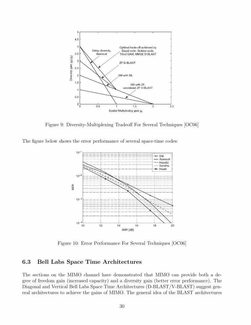
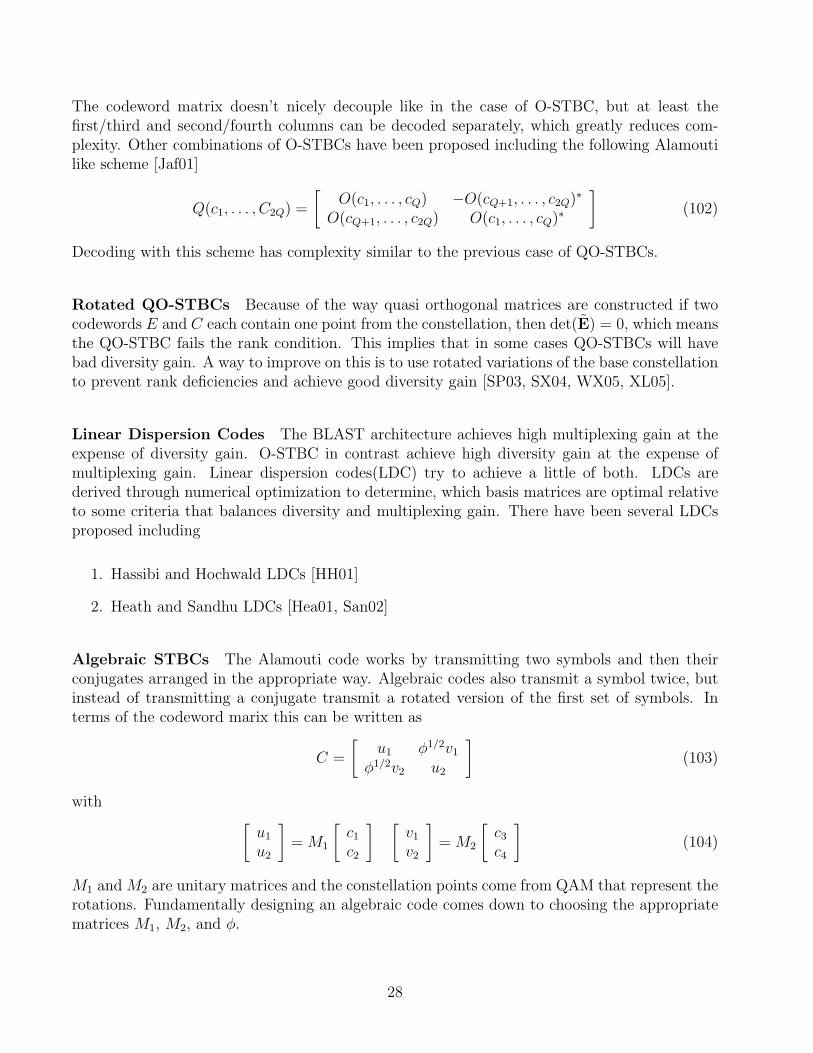
Figure 9: Diversity-Multiplexing Tradeoff For Several Techniques [OC06]
The figure below shows the error performance of several space-time codes:
Figure 10: Error Performance For Several Techniques [OC06]
6.3 Bell Labs Space Time Architectures
The sections on the MIMO channel have demonstrated that MIMO can provide both a de-gree of freedom gain (increased capacity) and a diversity gain (better error performance). TheDiagonal and Vertical Bell Labs Space Time Architectures (D-BLAST/V-BLAST) suggest gen-eral architectures to achieve the gains of MIMO. The general idea of the BLAST architectures
30

is to multiplex several streams of symbols (possibly demultiplexed from one original stream)onto the multiple antennas and then receive and decode the streams. Historically, G. Foschinisuggested the D-BLAST architecture first and then V-BLAST was developed later as a simplifi-cation. However, logically it makes more sense to present V-BLAST first and then discuss howD-BLAST is logically an extension of V-BLAST.
6.3.1 V-BLAST
The general architecture of V-BLAST is described in the figure below [GFVW99]
Figure 11: VBLAST Architecture
The independent streams are multiplexed by the matrix Q onto the transmit antennas. At thereceiver the streams are decoded jointly or individually. In V-BLAST there is a large degree offreedom in choosing the exact receiver structure. The choice of receiver structure affects errorrates, capacity, and the complexity of decoding. The design of efficient V-BLAST receivers isan active area of research.
There are two natural choices for Q depending on whether there is CSIT or not. If there isCSIT, then the matrix V from the SVD of H can be used. At the receiver the received vector yis multiplied by the matrix U from the SVD of H. These actions create an equivalent channelmodel:
y = Σx + v (110)
The complex MIMO channel is reduced to several parallel scalar channels with each subchannelcarrying one stream. The action of Q is to rotate the input streams, so that the action ofthe channel can be expressed in a simple form. Sometimes a system provides a codebook ofQ matrices that the transmitter can use. The feedback from receiver is just an index into thecodebook that tells the transmitter, which Q to use. This form of feedback massively reducesthe required bandwidth in the feedback channel.
If there is not CSIT, then the situation is considerably more complicated and interesting. In thiscase the best choice for Q is simply the identity matrix Int . In this case the choice of receiveris an interesting problem and there are many choices all with different choices.
V-BLAST Receiver Structures There are two general steps in the V-BLAST receiver. Thefirst is demodulation in which the receiver estimates what symbol was sent and hence which bitswere sent. The next step is decoding in which any codes that were applied to individual streams
31
are decoded. Basically any convolutional and block code can be applied to individual stream, sowe are primarily interested in different architectures for demodulation. The optimal V-BLASTreceiver is the ML-receiver that jointly decodes the streams. The ML receiver estimates thetransmitted streams by the rule [TV05]
s = arg mins∈C
||y −Hs||2 (111)
Practically what this method does is pick the closest point to the received vector in the lattice ofpoints formed by Hs, where s is a point in the original constellation. This problem is known asthe integer least squares problem. Although this method is optimal it is computationally complex(NP-hard) as it must be performed over all possible transmit vectors. This computationalcomplexity generally makes it infeasible to use an ML detector.
Sphere Decoding Although the ML detector is basically computationally infeasible in manypractical system there has been considerable interest in algorithms that are similar to ML-detection in methodology and performance but with considerably less complexity. In addition,these ML-like algorithms can feed soft decisions to the decoders to improve their performance.Sphere decoding is one such algorithm [VB99].
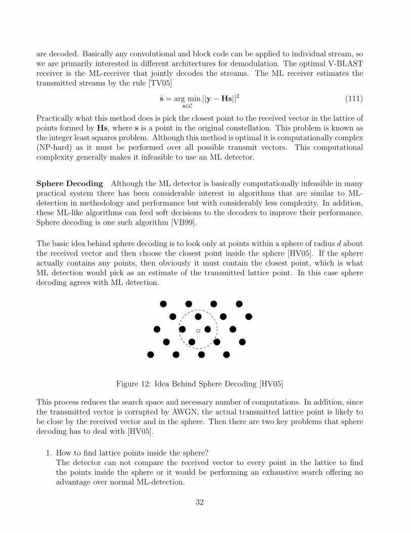
The basic idea behind sphere decoding is to look only at points within a sphere of radius d aboutthe received vector and then choose the closest point inside the sphere [HV05]. If the sphereactually contains any points, then obviously it must contain the closest point, which is whatML detection would pick as an estimate of the transmitted lattice point. In this case spheredecoding agrees with ML detection.
Figure 12: Idea Behind Sphere Decoding [HV05]
This process reduces the search space and necessary number of computations. In addition, sincethe transmitted vector is corrupted by AWGN, the actual transmitted lattice point is likely tobe close by the received vector and in the sphere. Then there are two key problems that spheredecoding has to deal with [HV05].
1. How to find lattice points inside the sphere?The detector can not compare the received vector to every point in the lattice to findthe points inside the sphere or it would be performing an exhaustive search offering noadvantage over normal ML-detection.
32
2. How to choose the sphere radius?If d is too large, then the detector considers too many points. If d is too small, then thesphere may contain no points. One way to choose the sphere radius is to compute theBabai estimate for the transmitted symbol sB. This estimate is not actually a point inthe lattice, but the least squares solution (not constrained to the lattice) given by
sB = arg mins
||y −Hs||2 (112)
Then choose d = ||y −HsB. There are other heurestic methods to choose d.
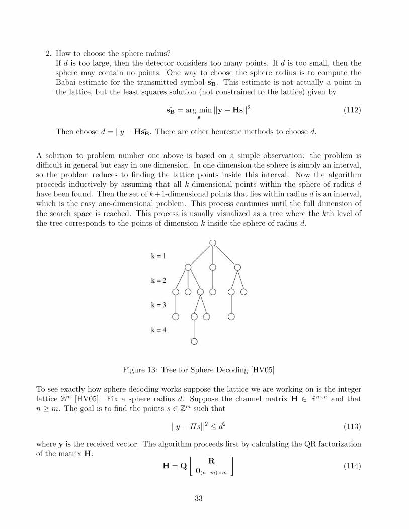
A solution to problem number one above is based on a simple observation: the problem isdifficult in general but easy in one dimension. In one dimension the sphere is simply an interval,so the problem reduces to finding the lattice points inside this interval. Now the algorithmproceeds inductively by assuming that all k-dimensional points within the sphere of radius dhave been found. Then the set of k+1-dimensional points that lies within radius d is an interval,which is the easy one-dimensional problem. This process continues until the full dimension ofthe search space is reached. This process is usually visualized as a tree where the kth level ofthe tree corresponds to the points of dimension k inside the sphere of radius d.
Figure 13: Tree for Sphere Decoding [HV05]
To see exactly how sphere decoding works suppose the lattice we are working on is the integerlattice Zm [HV05]. Fix a sphere radius d. Suppose the channel matrix H ∈ Rn×n and thatn ≥ m. The goal is to find the points s ∈ Zm such that
||y −Hs||2 ≤ d2 (113)
where y is the received vector. The algorithm proceeds first by calculating the QR factorizationof the matrix H:
H = Q
[R
0(n−m)×m
](114)
33
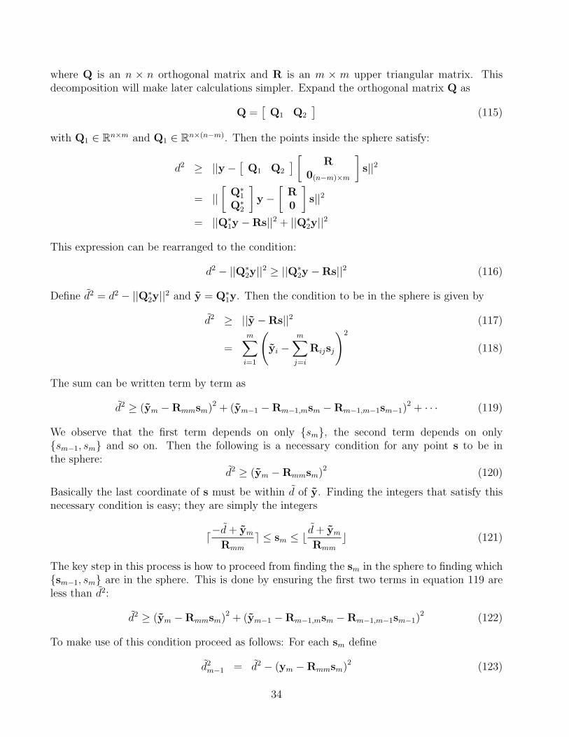
where Q is an n × n orthogonal matrix and R is an m × m upper triangular matrix. Thisdecomposition will make later calculations simpler. Expand the orthogonal matrix Q as
Q =[
Q1 Q2
](115)
with Q1 ∈ Rn×m and Q1 ∈ Rn×(n−m). Then the points inside the sphere satisfy:
d2 ≥ ||y −[
Q1 Q2
] [ R0(n−m)×m
]s||2
= ||[
Q∗1
Q∗2
]y −
[R0
]s||2
= ||Q∗1y −Rs||2 + ||Q∗
2y||2
This expression can be rearranged to the condition:
d2 − ||Q∗2y||2 ≥ ||Q∗
2y −Rs||2 (116)
Define d2 = d2 − ||Q∗2y||2 and y = Q∗
1y. Then the condition to be in the sphere is given by
d2 ≥ ||y −Rs||2 (117)
=m∑
i=1
(yi −
m∑j=i
Rijsj
)2
(118)
The sum can be written term by term as
d2 ≥ (ym −Rmmsm)2 + (ym−1 −Rm−1,msm −Rm−1,m−1sm−1)2 + · · · (119)
We observe that the first term depends on only sm, the second term depends on onlysm−1, sm and so on. Then the following is a necessary condition for any point s to be inthe sphere:
d2 ≥ (ym −Rmmsm)2 (120)
Basically the last coordinate of s must be within d of y. Finding the integers that satisfy thisnecessary condition is easy; they are simply the integers
d−d + ym
Rmm
e ≤ sm ≤ b d + ym
Rmm
c (121)
The key step in this process is how to proceed from finding the sm in the sphere to finding whichsm−1, sm are in the sphere. This is done by ensuring the first two terms in equation 119 areless than d2:
d2 ≥ (ym −Rmmsm)2 + (ym−1 −Rm−1,msm −Rm−1,m−1sm−1)2 (122)
To make use of this condition proceed as follows: For each sm define
d2m−1 = d2 − (ym −Rmmsm)2 (123)
34

Then we can obtain a condition that sm−1 must satisfy to be in the sphere:
d−dm−1 + ym−1 −Rm−1,msm
Rm−1,m−1
e ≤ sm−1 ≤ b dm−1 + ym−1 −Rm−1,msm
Rm−1,m−1
c (124)
By applying this method to each sm the points sm−1, sm inside the sphere of radius d can befound. This process can be continued until the full m-dimensional problem has been solved. Itis clear why a tree is an appropriate structure to represent the operation of sphere decoding,since each leaf gives rise to some number of children (possibly zero) in the next iteration allof whom are inside the sphere as one more dimension of the problem is solved. It is also clearthat if we choose the radius to be too small one of the conditions like equation 124 may not besatisfied by any integer and thus no points are in the sphere. If the sphere radius is too large,then too many points may satisfy equation 124 making computing the closest point tricky.
Non-Joint Detection Besides joint detection there are a wealth of detectors that work ondetecting individual streams from the received signal and don’t attempt to decode all the streamssimultaneously. Consider trying to decode one stream xk. The system in this case can bemodeled as
y[n] = hkxk[n] +∑i6=k
hixi[n] + v[n] (125)
where hi is the ith column of the channel matrix H. In this system there is a stream of interestplus several interfering streams represented by the sum terms plus a noise terms. To successfullydecode the stream of interest the receiver must deal with the interference term and the noiseterm.
Zero Forcing Nulling At high SNR performance will be interference limited not noise limited[GFVW99]. ZF-Nulling attempts to remove all the interfering terms in the sum to leave only thestream of interest. This can be done linearly with a single vector multiplication. The weightingvector qk to decode the kth stream satisfies
qTk hj = δkj (126)
where δkj is the Kronecker delta which is 1 when k = j and 0 otherwise. Then
qTk y[n] = qT
k hkxk[n] +∑i6=k
qTk hixi[n] + qT
k v[n]
= δkkxk[n] +∑i6=k
δkixi[n] + qTk v[n]
= xk[n] + qTk v[n]
This weighting vector has an obvious geometric interpretation; the weighting vector projects thereceived vector y onto a subspace orthogonal to h1, . . . ,hk−1,hk+1, . . . ,hnt .
35
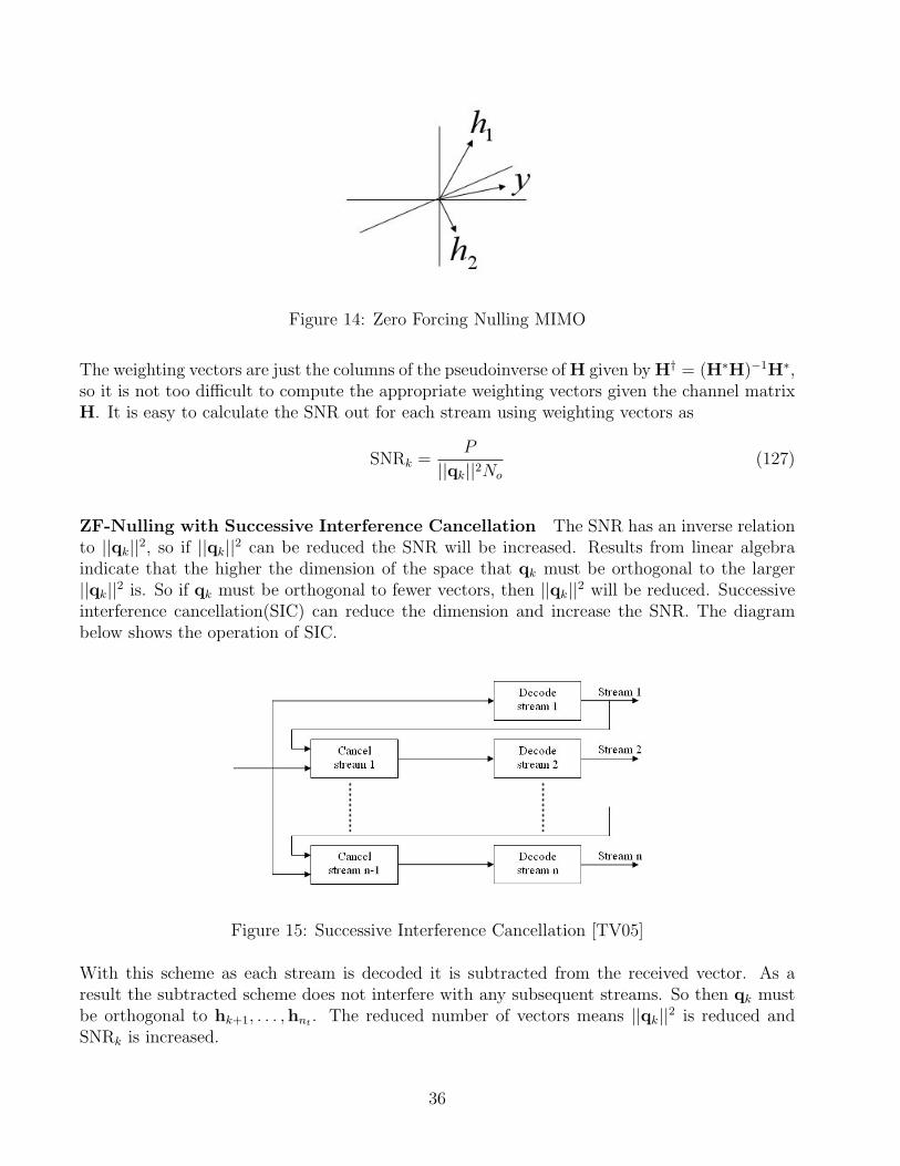
Figure 14: Zero Forcing Nulling MIMO
The weighting vectors are just the columns of the pseudoinverse of H given by H† = (H∗H)−1H∗,so it is not too difficult to compute the appropriate weighting vectors given the channel matrixH. It is easy to calculate the SNR out for each stream using weighting vectors as
SNRk =P
||qk||2No
(127)
ZF-Nulling with Successive Interference Cancellation The SNR has an inverse relationto ||qk||2, so if ||qk||2 can be reduced the SNR will be increased. Results from linear algebraindicate that the higher the dimension of the space that qk must be orthogonal to the larger||qk||2 is. So if qk must be orthogonal to fewer vectors, then ||qk||2 will be reduced. Successiveinterference cancellation(SIC) can reduce the dimension and increase the SNR. The diagrambelow shows the operation of SIC.
Figure 15: Successive Interference Cancellation [TV05]
With this scheme as each stream is decoded it is subtracted from the received vector. As aresult the subtracted scheme does not interfere with any subsequent streams. So then qk mustbe orthogonal to hk+1, . . . ,hnt . The reduced number of vectors means ||qk||2 is reduced andSNRk is increased.
36
One practical issue when implementing SIC is the order of cancellation. The last decoded streamhas the least interference and achieves the best performance. It has been demonstrated that agreedy choice of order is optimal relative to the maximin criteria [GFVW99]. This means thatthe kth stream to be decoded should be chosen from the reaming streams as the one that willachieve the highest SNR of the remaining streams if it is decoded now. The maximin criteriameans that the smallest SNRk is maximized by choosing the optimal order.
The major drawback to SIC is error propagation. Mistakes at the beginning of the decoding chaincan introduce mistakes later on. So if one stream is inaccurately decoded, then all subsequentstreams will likely be decoded inaccurately.
Matched Filter At very low SNR noise is the problem, so a matched filter can be used todeal with the noise. In the MIMO case the matched filter for each stream is simply maximumratio combining(MRC) performed on the appropriate column of H.
MMSE Receiver The matched filter performs well at low SNR and ZF-nulling performs wellat high SNR. But at high SNR the matched filter has bad performance and at low SNR ZF-nulling has bad performance. So naturally one may wonder if there is a receiver that operateswell at both low and high SNR. The MMSE receiver is such a receiver [TV05].
To understand how the MMSE receiver works consider the following SIMO system modeled as
y = hx + z (128)
with z colored noise having invertible correlation matrix Kz. The first operation is to whiten
the noise by multiplying by K− 1
2z . Then the system becomes
K− 1
2z y = K
− 12
z hx + K− 1
2z z (129)
Then apply a matched filter (K− 1
2z h)∗ to yield the system
h∗K−1z y = (h∗K−1
z h)x + h∗K−1z z (130)
Thus the receiver simply multiplies the received signal by h∗K−1z and performs normal demod-
ulation. This is the MMSE receiver, which maximizes the SNR, while minimizing the MMSEbetween the estimate of x and x itself.
For V-BLAST the corrupting non-white noise is the interference terms plus the additive noise.The covariance matrix for this noise is given by
Kzk= NoInr +
∑i6=k
Pihih∗i (131)
A similar derivation shows that the MMSE receiver in this case the weighting vector is
qk =
(NoInr +
∑i6=k
Pihih∗i
)−1
hk (132)
37
It is pretty easy to see that the MMSE receiver is a tradeoff between the matched filter andZF-Nulling. At low SNR
Kzk≈ NoInr (133)
so the receiver is given by hk, which is a matched filter. At high SNR
Kzk≈∑i6=k
Pihih∗i (134)
and it can be seen that qk is simply the kth column of the pseudoinverse of H. Thus the MMSEreceiver is like ZF-Nulling at high SNR. In addition, the MMSE receiver has good performancein the region between high and low SNR. If SIC is used in conjunction with MMSE, thenMMSE-SIC can achieve the channel capacity.
6.3.2 D-BLAST
Consider the kth stream. It is transmitted by one antenna and received by all nr receiveantennas. Thus the maximum possible diversity gain for any individual stream is nr and thereis a limit to how much MIMO diversity techniques can protect a stream [Fos96]. If a SICstructure is used with either the MMSE receiver or ZF-nulling, then if one stream is incorrectlydecoded, then subsequent streams will likely be incorrectly decoded. The main reason for thisproblem is that no coding is performed spatially across the multiple streams. Coding acrossstreams is used to ensure each stream is reliably decoded, but in order to decode the spatialcode across the streams each stream must already be decoded in V-BLAST. The solution to thisproblem is to alter the way the streams are transmitted.
Consider the case with two transmit antennas. Suppose that there are two separate streamseach consisting of two blocks. Denote this by a(i) and b(i) for i = 0, 1. Then the D-BLASTcodeword is
C =
[a(1) b(1)
a(2) b(2)
](135)
From this codeword matrix it is obvious where D-BLAST gets its name from, since the layersare now diagonal. The receiver works as follows:
1. First receive a(1) with MRC
2. Next receive a(2) with MMSE or ZF-nulling, while ignoring b(1).
3. Next decode the spatial code across the first layer [a(1) a(2)].
4. Now a(2) has been reliably decoded, so it can be cancelled out and b(1) can be received.
5. Finally, b(2) can be received with MRC. Then the second layer [b(1) b(2)] can be decoded.
Now both streams have been decoded reliably. The key observation is that for a single layerif one of the blocks for one stream is initially decoded incorrectly, there is still a chance to fix
38
the error with the code applied across the layer. The major price to pay for using D-BLASTis the lost capacity during the startup process due to the blank spots in the codeword. Forexample, during the first block the second transmit antenna transmits nothing, and so somecapacity is lost. Finally, there is also the cost in implementation complexity of applying codingand decoding across streams.
6.4 Space-Time Trellis Codes
A space-time trellis code (STTC) is an extension of normal convolutional codes to multipleantennas [TSC98]. The key idea behind a STTC is to make the output of the encoder a functionof the input bits and the state of the encoder, which is in turn a function of the previous inputs.Trellis codes provide better error performance compared to block codes and coding gain at theexpense of implementation complexity.
6.4.1 Trellis Representation
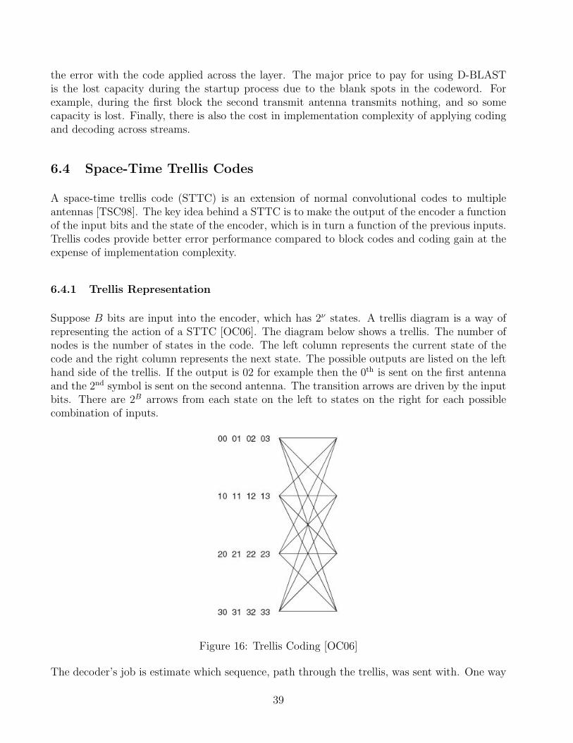
Suppose B bits are input into the encoder, which has 2ν states. A trellis diagram is a way ofrepresenting the action of a STTC [OC06]. The diagram below shows a trellis. The number ofnodes is the number of states in the code. The left column represents the current state of thecode and the right column represents the next state. The possible outputs are listed on the lefthand side of the trellis. If the output is 02 for example then the 0th is sent on the first antennaand the 2nd symbol is sent on the second antenna. The transition arrows are driven by the inputbits. There are 2B arrows from each state on the left to states on the right for each possiblecombination of inputs.
Figure 16: Trellis Coding [OC06]
The decoder’s job is estimate which sequence, path through the trellis, was sent with. One way
39
to do this is with a Maximum Likelihood Sequence Estimator (MLSE). There is a well knownalgorithm - the Viterbi algorithm - to efficiently estimate, which sequence was sent.
Trellis Complexity There is a fundamental lower bound to the complexity of a STTC. For aSTTC with B input bits and minimum rank rmin has at least 2B(rmin−1) states. Obviously as thenumber of states increases the complexity of decoding increases, so this lower bound on statesputs a lower bound on the possible complexity.
6.4.2 Delay-Diversity Scheme
This is one of the simplest trellis codes to achieve diversity [Wit93, SW94]. The codeword forT transmitted symbols is given by
C =1√2
[c1 c2 · · · cT 00 c1 · · · cT−1 cT
](136)
The trellis diagram below represents this code
The effect of this code is to convert spatial diversity to frequency diversity. Consider a 2 × 1MIMO system. When c1 is transmitted during the first symbol period, it sees the channel h1.When c1 is transmitted during the second symbol period, it sees channel h2. This is equivalentto passing c1 through a frequency selective channel with two taps in the frequency domain: h1
and h2. So spatial diversity becomes frequency diversity by applying this code.
7 Space-Time Coding for Frequency Selective Channels
There are two basic approaches to MIMO over frequency selective channels as in normal SISOfrequency selective channels:
1. Single carrier
2. Multicarrier - OFDM
Many modern wireless standards that use MIMO also use OFDM, so MIMO-OFDM is of par-ticular interest.
7.1 Single Carrier
In this case the system can be modeled as
yk =L−1∑l=0
H[l]ck−l + vk (137)
40

This complicated system involving a summation can be expressed as a simple system of the form
yk = [H[0] · · ·H[L− 1]][cT
k · · · cTk−L+1
]T+ vk (138)
which is similar to the narrowband MIMO case.
7.2 MIMO-OFDM
MIMO-OFDM is an extension of normal OFDM to the MIMO case where there are multipleantennas.
7.2.1 OFDM
OFDM uses the FFT and IFFT to decompose the wideband frequency selective channel intoseveral smaller narrowband frequency flat channels. The cyclic prefix is added to prevent ISI.
Figure 17: OFDM System Model [OC06]
The system model can be expressed in the DFT frequency domain as
Y [k] = H[k]X[k] + V [k] (139)
with V [k] the corrupting noise. H[k]X[k] results in a circular convolution in the time domain,which can be expressed in matrix form as
y[0]y[1]...
y[N − 1]
=
h[0] h[N − 1] h[N − 2] · · · h[1]h[1] h[0] h[N − 1] · · · [2]
......
.... . .
...h[N − 1] h[N − 2] h[N − 3] · · · h[1]
x[0]x[1]
...x[N − 1]
+
v[0]v[1]...
v[N − 1]
The singular value decomposition of H is DΛD∗. Where D is the matrix that performs theDFT. The matrix Λ is a diagonal matrix specific to each H
Λ =
λ1 0
λ2
. . .
0 λN
(140)
but D is not specific to each H.
41
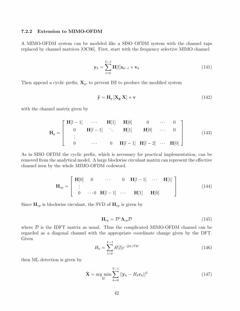
7.2.2 Extension to MIMO-OFDM
A MIMO-OFDM system can be modeled like a SISO OFDM system with the channel tapsreplaced by channel matrices [OC06]. First, start with the frequency selective MIMO channel
yk =L−1∑l=0
H[l]xk−l + vk (141)
Then append a cyclic prefix, Xg, to prevent ISI to produce the modified system
y = Hg [Xg X] + v (142)
with the channel matrix given by
Hg =
H[l − 1] · · · H[1] H[0] 0 · · · 0
0 H[l − 1]. . . H[1] H[0] · · · 0
...0 · · · 0 H[l − 1] H[l − 2] · · · H[0]
(143)
As in SISO OFDM the cyclic prefix, which is necessary for practical implementation, can beremoved from the analytical model. A large blockwise circulant matrix can represent the effectivechannel seen by the whole MIMO-OFDM codeword.
Hcp =
H[0] 0 · · · 0 H[l − 1] · · · H[1]...0 · · · 0 H[l − 1] · · · H[1] H[0]
(144)
Since Hcp is blockwise circulant, the SVD of Hcp is given by
Hcp = D∗ΛcpD (145)
where D is the IDFT matrix as usual. Thus the complicated MIMO-OFDM channel can beregarded as a diagonal channel with the appropriate coordinate change given by the DFT.Given
Hk =L−1∑l=0
H[l]e−j2π/Tkl (146)
then ML detection is given by
X = arg minC
T−1∑k=0
||yk −Hkck||2 (147)
42
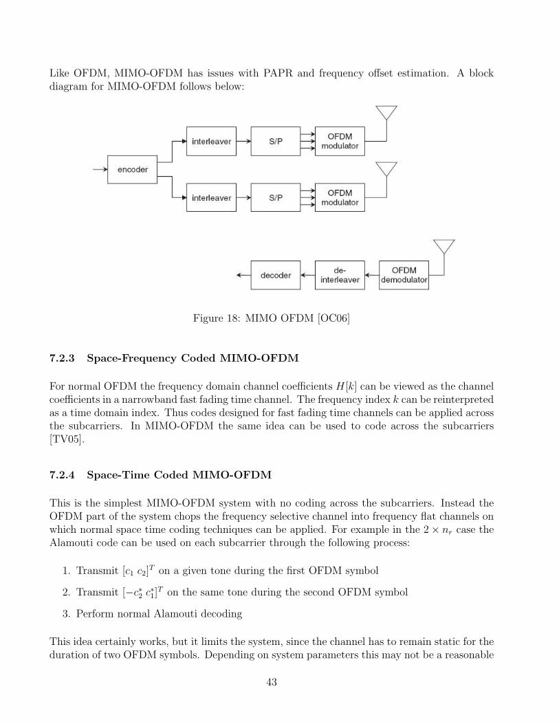
Like OFDM, MIMO-OFDM has issues with PAPR and frequency offset estimation. A blockdiagram for MIMO-OFDM follows below:
Figure 18: MIMO OFDM [OC06]
7.2.3 Space-Frequency Coded MIMO-OFDM
For normal OFDM the frequency domain channel coefficients H[k] can be viewed as the channelcoefficients in a narrowband fast fading time channel. The frequency index k can be reinterpretedas a time domain index. Thus codes designed for fast fading time channels can be applied acrossthe subcarriers. In MIMO-OFDM the same idea can be used to code across the subcarriers[TV05].
7.2.4 Space-Time Coded MIMO-OFDM
This is the simplest MIMO-OFDM system with no coding across the subcarriers. Instead theOFDM part of the system chops the frequency selective channel into frequency flat channels onwhich normal space time coding techniques can be applied. For example in the 2× nr case theAlamouti code can be used on each subcarrier through the following process:
1. Transmit [c1 c2]T on a given tone during the first OFDM symbol
2. Transmit [−c∗2 c∗1]T on the same tone during the second OFDM symbol
3. Perform normal Alamouti decoding
This idea certainly works, but it limits the system, since the channel has to remain static for theduration of two OFDM symbols. Depending on system parameters this may not be a reasonable
43
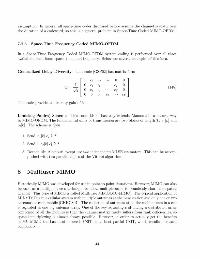
assumption. In general all space-time codes discussed before assume the channel is static overthe duration of a codeword, so this is a general problem in Space-Time Coded MIMO-OFDM.
7.2.5 Space-Time Frequency Coded MIMO-OFDM
In a Space-Time Frequency Coded MIMO-OFDM system coding is performed over all threeavailable dimensions: space, time, and frequency. Below are several examples of this idea.
Generalized Delay Diversity This code [GSP02] has matrix form
C =1√2
c1 c2 · · · cT 0 00 c1 c2 · · · cT 00 c1 c2 · · · cT 00 0 c1 c2 · · · cT
(148)
This code provides a diversity gain of 3.
Lindskog-Paulraj Scheme This code [LP00] basically extends Alamouti in a natural wayto MIMO-OFDM. The fundamental units of transmission are two blocks of length T : c1[k] andc2[k]. The scheme is then
1. Send [c1[k] c2[k]]T
2. Send [−c∗2[k] c∗1[k]]T
3. Decode like Alamouti except use two independent MLSE estimators. This can be accom-plished with two parallel copies of the Viterbi algorithm.
8 Multiuser MIMO
Historically MIMO was developed for use in point to point situations. However, MIMO can alsobe used as a multiple access technique to allow multiple users to seamlessly share the spatialchannel. This type of MIMO is called Multiuser MIMO(MU-MIMO). The typical application ofMU-MIMO is in a cellular system with multiple antennas at the base station and only one or twoantennas at each mobile [GKHCS07]. The collection of antennas at all the mobile users in a cellis regarded as one big antenna array. One of the key advantages of having a distributed arraycomprised of all the mobiles is that the channel matrix rarely suffers from rank deficiencies, sospatial multiplexing is almost always possible. However, in order to actually get the benefitsof MU-MIMO the base station needs CSIT or at least partial CSIT, which entails increasedcomplexity.
44

For a MU-MIMO system having N transmit antennas at the base station and U users each withMk antenna the downlink, broadcast channel, for each user can be modeled as
yk = hk
N∑l=1
xl + vk (149)
The uplink, MAC channel, can be modeled as
y =U∑
i=1
hkxk + v (150)
8.1 Precoding
Information theoretic results have shown that using a type of coding called dirty paper cod-ing(DPC) at the transmitter N users streams can be multiplexed and transmitted [SB07, GC80].Effectively what the coding at the transmitter does is pre-cancel out interference at the receiverslike ZF-nulling does in BLAST.
8.1.1 Linear Precoding
The downlink channel can be written in a simple for making explicit how other users’ streamsproduce interference.
yk = Hksk + Hk
N∑l=1,l 6=k
sk + vk (151)
The simplest form of precoding is to multiply the transmit symbols by a matrix, Wk, that willcancel out the interferers [SSH04].
yk = HkWksk + Hk
N∑l=1,l 6=k
Wlsk + vk (152)
In the case when each user has one receive antenna this problem is identical to canceling inter-ference in BLAST. So the proper choice for Wk is the kth column of the pseudoinverse of theeffective channel matrix H =
[h1 h1 · · · hN
].
8.1.2 Nonlinear Precoding
Nonlinear precoding is more like DPC than linear precoding and can produce better results atthe cost of increased complexity. Well known nonlinear precoding methods include perturbationmethods and Tomlinson-Harathisma codes [PHS05, HPS05].
45

8.2 Scheduling
If the number of users U is greater than the number of transmit antennas N , then the basestation can’t transmit to all the users simultaneously. So at any given time the base stationmust choose some subset of the users to transmit to [GKHCS07]. The optimal schedulingalgorithm is to simply perform an exhaustive search over all possible combinations of users.This is not computationally feasible though, so heurestic methods must be used to choose asubset of users. A simple choice is a greedy algorithm, which selects the N users with the bestchannels.
8.3 Working with Partial CSIT
To achieve CSIT each user must feedback its channel estimate to the base station, which is trickyand reduces capacity [GA04]. To combat this problem some research has been performed intoMU-MIMO systems with only partial CSIT. Basic results have demonstrated that the gains ofMU-MIMO can still be achieved with only partial CSIT, which entails less system complexity.
9 MIMO in Wireless Standards
Many emerging wireless standards provide for MIMO to provide both diversity and multiplexinggain as needed. This section examines three prominent new wireless standards that employMIMO.
9.1 3GPP LTE
The Third Generation Partnership Project Long-Term Evolution (3GPP LTE) is the emerging4G standard that is currently being implemented and tested. The major features of LTE areoutlined below [3GPP07, 3GPPRel8, 3GPPRel9]:
• High data rates - 100 Mbps in the downlink using 2× 2 MIMO and 50 Mbps in the uplinkusing no MIMO
• Mobility - Best performance for 0-15 km/hr and good performance of 15-120 km/hr.
• Spectrum - No fixed spectrum size. Allowed sizes are 1.25, 1.6, 2.5, 5, 10, 15, and 20 MHz.
• OFDM - LTE uses OFDM with a variable number of subcarriers.
• IP Network - No circuit switched domain but all IP based network.
The downlink in LTE provides several options for using MIMO. The basic option for the downlinkis two antennas at the base station and two at the mobile station. Extensions to LTE allow4× 2 and 4× 4 MIMO. If the base station has CSIT, then there are two methods it can apply:
46
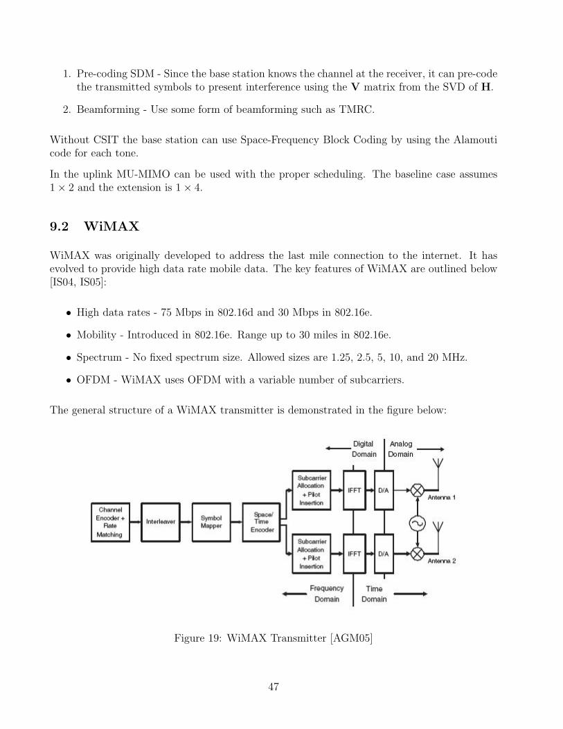
1. Pre-coding SDM - Since the base station knows the channel at the receiver, it can pre-codethe transmitted symbols to present interference using the V matrix from the SVD of H.
2. Beamforming - Use some form of beamforming such as TMRC.
Without CSIT the base station can use Space-Frequency Block Coding by using the Alamouticode for each tone.
In the uplink MU-MIMO can be used with the proper scheduling. The baseline case assumes1× 2 and the extension is 1× 4.
9.2 WiMAX
WiMAX was originally developed to address the last mile connection to the internet. It hasevolved to provide high data rate mobile data. The key features of WiMAX are outlined below[IS04, IS05]:
• High data rates - 75 Mbps in 802.16d and 30 Mbps in 802.16e.
• Mobility - Introduced in 802.16e. Range up to 30 miles in 802.16e.
• Spectrum - No fixed spectrum size. Allowed sizes are 1.25, 2.5, 5, 10, and 20 MHz.
• OFDM - WiMAX uses OFDM with a variable number of subcarriers.
The general structure of a WiMAX transmitter is demonstrated in the figure below:
Figure 19: WiMAX Transmitter [AGM05]
47

There are several different MIMO methods that can be employed in WiMAX. As we have seenbefore the methods employed depend on whether the transmitter has channel state informationor not.
Open Loop (No CSIT) The 802.16 standard defines several options for space-time codesfor 2-4 antennas. However, the two most common codes for space-time coding are:[
S1
S2
] [S1 −S∗2S2 S∗1
](153)
where S1 and S2 are OFDM symbols. 802.16 also provides for space-frequency coding called theFrequency Hopping Diversity Code (FHDC) based on the Alamouti code. The OFDM symbolsare uncoded in time and coded in the frequency domain. The figure below shows how FHDCworks:
Figure 20: WiMAX Frequency Hopping Diversity [AGM05]
Closed Loop (CSIT) With CSIT the transmitter can make better decisions. One of thecommon methods used in feedback is codebook based feedback. The codebook is basically apredetermined set of choices for the Q matrix in BLAST. The feedback is an index into thecodebook that tells the receiver, which matrix to use. Another alternative is to use a feedbackchannel and have the receiver transmit a quantized version of the channel. The transmitter canthen design the optimal precoding matrix.
9.3 802.11n
802.11n is the next generation 802.11 LAN that seeks to provide very high data rates. In 802.11a/b/g high data rates were achieved by using high order modulation like 64-QAM. However,the cost of this approach is a loss in range because higher SNR is necessary to successfullydemodulate 64-QAM. The way 802.11n seeks to overcome this problem and provide both high
48
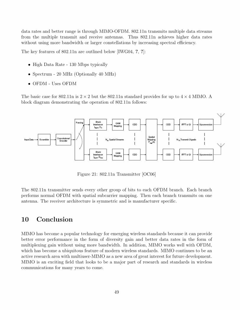
data rates and better range is through MIMO-OFDM. 802.11n transmits multiple data streamsfrom the multiple transmit and receive antennas. Thus 802.11n achieves higher data rateswithout using more bandwidth or larger constellations by increasing spectral efficiency.
The key features of 802.11n are outlined below [IWG04, ?, ?]:
• High Data Rate - 130 Mbps typically
• Spectrum - 20 MHz (Optionally 40 MHz)
• OFDM - Uses OFDM
The basic case for 802.11n is 2× 2 but the 802.11n standard provides for up to 4× 4 MIMO. Ablock diagram demonstrating the operation of 802.11n follows:
Figure 21: 802.11n Transmitter [OC06]
The 802.11n transmitter sends every other group of bits to each OFDM branch. Each branchperforms normal OFDM with spatial subcarrier mapping. Then each branch transmits on oneantenna. The receiver architecture is symmetric and is manufacturer specific.
10 Conclusion
MIMO has become a popular technology for emerging wireless standards because it can providebetter error performance in the form of diversity gain and better data rates in the form ofmultiplexing gain without using more bandwidth. In addition, MIMO works well with OFDM,which has become a ubiquitous feature of modern wireless standards. MIMO continues to be anactive research area with multiuser-MIMO as a new area of great interest for future development.MIMO is an exciting field that looks to be a major part of research and standards in wirelesscommunications for many years to come.
49

A Math Review
This section reviews a few common mathematical tools used in MIMO. In particular, this sectioncovers some important linear algebra topics and Lagrange multipliers for optimization [HJ95].
A.1 Rank
Let A ∈ Cm×n. Then A can be written in terms of column vectors as A = [a1, a2, . . . , an]. Thecolumn space of A denoted col(A) is given by
col(A) = span(a1, a2, . . . , an) (154)
Then the rank of A denoted rank(A) is defined to be dim col(A). So the rank of A is the largestnumber of columns of A that constitute a linearly independent set.
A can be written in terms of rows as [a′T1 , a′T2 , . . . , a′Tm ]T. Then the row space of A denotedrow(A) is given by
row(A) = span(a′1, a′2, . . . , a
′n) (155)
With these definitions it can be demonstrated that rank(A) = dim row(A). Listed below areseveral useful facts about rank:
1. rank(AT) = rank(A∗) = rank(A)
2. rank(A) ≤ minm,n.
3. rank(A∗A) = rank(A)
4. If A is square, then A is invertible if and only if rank(A) = n.
A.2 Eigenvalues and Eigenvectors
Let A be a n×n matrix over the complex numbers. A complex number λ and a complex vectorx 6= 0 are said to be an eigenvalue and its associated eigenvector if
Ax = λx (156)
By simple rearranging this expression can be written as
(A− λI)x = 0 (157)
This equations has non-trivial solutions (x 6= 0) only if A − λI is not invertible. This is trueprecisely when det (A− λI) = 0. When the determinant is expanded and evaluated it becomesan nth degree polynomial. By the Fundamental Theorem of Algebra this polynomial has ncomplex roots counting multiplicity. Thus A has n eigenvalues including multiplicity.
50
A.2.1 Diagonalization
Sometimes A can be related to a diagonal matrix D by A = S−1DS where S is a n × ninvertible matrix. If this is possible, then A is said to be diagonalizable. The matrix S can beinterpreted as a change of basis that allows the matrix A to be described as a diagonal matrix.This representation is particularly nice in a n× n MIMO system, since the channel becomes nindependent parallel channels. This transformation makes capacity calculation much easier.
So the main point of interest is determining when A is diagonalizable. The following twoconditions are sufficient to guarantee that a square matrix is diagonalizable:
1. A has n distinct eigenvalues
2. A has n linearly independent eigenvalues
A.2.2 Connection To The Determinant and Trace
The following formula is a useful connection between the eigenvalues of a matrix and its deter-minant and trace:
det(A) = λ1λ2 · · ·λn (158)
tr(A) =n∑
i=1
aii = λ1 + λ2 + · · ·+ λn (159)
A.3 Inner Product Space
Cn×1 is an inner product space with the inner product given by:
< x,y >= y∗x (160)
There are two important points of interest in regarding Cn×1 as an inner product space. First, itis possible to perform orthogonal projections of a vector onto a space spanned by several othervectors. This can be used in V-BLAST for the ZF-Nulling receiver. The second point is theCauchy-Schwarz inequality
| < x,y > | ≤√
< x,x >√
< y,y > (161)
with equality for y = Kx for any constant K. The Cauchy-Schwarz inequality can be used toderive the optimal receive combining vector for MRC.
A.4 Singular Value Decomposition
It is only possible to diagonalize a square matrix, but sometimes it is desirable to decompose amatrix with arbitrary dimensions into another matrix that is almost diagonal. The singular value
51
decomposition achieves this and is defined for all matrices in Cm×n. Specifically the singularvalue decomposition of a matrix A ∈ Cm×n is
A = UΣV∗ (162)
where U ∈ Cm×m and V ∈ Cn×n are unitary matrices, which means
UU∗ = U∗U = Im (163)
VV∗ = V∗V = In (164)
Σ ∈ Cm×n has non-zero entries only for the entries on the diagonal, Σii. The entries Σii arecalled the singular values of A. Then it is clear that there are nmin = minm, n singular values.Typically the matrix Σ is constructed such that
Σ11 ≥ Σ22 ≥ · · · ≥ Σnminnmin(165)
Intuitively what the SVD does is use the matrix V to rotate an input vector to a coordinatesystem in which the action of the matrix can be described by a simple matrix Σ. Then theoutput of this simple matrix is rotated back to the original coordinate system by U to producethe output of A.
The concept of the SVD can be viewed as a generalization of eigenvalues. For a column ofu ∈ Cm, a corresponding column of v ∈ Cn, and the corresponding singular value σ ∈ C
Av = σu (166)
This equation is similar to the equation that defines an eigenvalue and eigenvector, which led tou being called a left singular vector and v a right singular vector. One of the most importantproperties of the SVD is that the number of non-zero singular values is precisely the rank of thematrix A.
A.4.1 Pseudoinverse
The inverse of a matrix is only defined for square matrices, but there is a way to define a specialmatrix that is like an inverse but defined for arbitrary m× n matrices called the pseudoinverse.Let A ∈ Cm×n have a SVD UΣV∗. Then the pseudoinverse is defined to be A† = VΣ†U∗
where Σ† is the transpose of Σ with the non-zero singular values inverted. There are four keryproperties of the pseudoinverse that define its behavior:
1. AA†A = A - Note that AA† is not in general the identity matrix but the combination ofthree matrices produces the desired effect.
2. A†AA† = A†
3.(AA†)∗ = AA†
4.(A†A
)∗= A†A
52
A.4.2 Condition Number
Consider solving the linear system Ax = b. The condition number is a measure of how well thissystem behaves for small changes in b. Specifically the condition number measures how smallchanges in b change x. So for the perturbed system Ax = b + e the condition number is givenby
κ(A) =||A−1e||/||A−1b
||e||/||b||(167)
This quantity can be related to the singular values of A by
κ(A) =σmax
σmin
(168)
A.5 Lagrange Multipliers
Consider the following optimization problem:
Maximize : f(x1, x2, . . . , xn)
Subject to : g(x1, x2, . . . , xn) = C
The optimal solution can be found by solving the following system of equations given by thegradient
5f = λ5g
g = C (169)
These equations can be expressed in terms of partial derivatives as
∂f
∂xi
= λ∂g
∂xi
i = 1, 2, . . . , n
g = C (170)
Lagrange multipliers can be used to find the optimal power allocation to maximize capacity.
References
[3GPPRel8] 3GPP, “Technical Specification Group Radio Access Network Requirements forFurther Advancements for E-UTRA (LTE-Advanced) (Release 8)”
[3GPPRel9] 3GPP. “Overview of 3GPP Release 9 V.0.0.4 (2009-01)”
[3GPP07] 3GPP. “Physical Channels and Modulation (Release 8)”. September 2007.
[AG05] J. Akhtar and D. Gesbert. “Spatial Multiplexing over correlated MIMO channels witha closed-form precoder”. IEEE Trans. Wireless Commun., 4(5):2400-2409, September 2005.
53
[AGM05] J. Andrews, A. Ghosh, and R. Muhamed. Fundamentals of WiMAX
[Ala98] S.M. Alamouti. “A simple transmit diversity technique for wireless communications”.IEEE J. Select. Areas Commun., 16(10):1451-1458, October 1998.
[BRV05] J.C. Belfiore, G. Rekaya, and E.Viterbo. “The golden code: a 22 full-rate space-timecode with non-vanishing determinants”. IEEE Trans. Inform. Theory, 51(4):1432-1436, April2005.
[CKT98] C.N. Chuah, J.M. Kahn, and D. Tse. “Capacity of multi-antenna array systems inindoor wireless environment”. In Proc. Globecom 1998 - IEEE Global TelecommunicationsConf., volume 4, pages 1894-1899, Sydney, Australia, 1998.
[CT91] T. Cover and T. Thomas. Elements of Information Theory. Wiley, NewYork, NY, 1991.
[DTB02] M.O. Damen,A.Tewfik, and J.-C. Belfiore. “A construction of a space-time code basedon number theory”. IEEE Trans. Inform. Theory, 48(3):753-760, March 2002.
[Fle00] B.H. Fleury. “First- and second-order characterization of direction dispersion and spaceselectivity in the radio channel”. IEEE Trans. Inform. Theory, 46(6):2027-2044, June 2000.
[FG98] G.J. Goschini and M.J. Gans. “On Limits of Wireless Communications in a FadingEnvironment when Using Multiple Antennas,” Wireless Personal Communications. Vol 6(3),March 1998.
[Fos96] G.J. Foschini. “Layered space-time architecture for wireless communication in a fadingenvironment when using multi-element antennas”. Bell Labs Tech. J., pages 41-59, Autumn1996.
[GA04] D. Gesbert and M.-S. Alouini, “How much feedback is multi-user diversity reallyworth?”, Proc. IEEE Int. Conf. on Comm. (ICC), Paris, France, June 2004, pp. 234-238
[GC80] A. El Gamal and T.M. Cover, “Multiple user information theory”, Proc. IEEE, vol. 68,no. 12, pp. 1466-1483, Dec. 1980
[GD03] H.E. Gamal and M.O. Damen. “Universal space-time coding”. IEEE Trans. Inform.Theory, 49(5):1097-1119, May 2003.
[GKHCS07] D. Gesbert, M. Kountouris, R. W. Heath, Jr., C.-B. Chae, and T. Salzer, “Shift-ing the MIMO Paradigm: From Single User to Multiuser Communications”, IEEE SignalProcessing Magazine, vol. 24, no. 5, pp. 36-46, Oct. 2007
[Gold05] Andrea Goldsmith. Wireless Communications. Cambridge Press. 2005.
[GFVW99] G.D. Golden, G.J. Foschini, R.A.Valenzuela, and P.W.Wolniansky. “Detection al-gorithm and initial laboratory results using the V-BLAST space- time communication ar-chitecture”. Elect. Lett., 35(1):14-15, January 1999.
54
[God97] L.C. Godara. “Applications of antenna arrays to mobile communications, part II:Beamforming and direction-of-arrival considerations”. Proceedings IEEE, 85(8):1195-1245,August 1997.
[GSP02] D. Gore, S. Sandhu, and A. Paulraj. “Delay diversity codes for frequency selectivechannels”. In Proc. ICC 2002 - IEEE Int. Conf. Commun., pages 1949-1953, NewYork, May2002.
[Hea01] R. Heath. “Space-Time Signaling in Multi-Antenna Systems”. PhD thesis, StanfordUniversity, November 2001.
[Her04] M. Herdin. “Non-stationary indoor MIMO radio channels”. PhD thesis, TechnischeUniversitatWien, August 2004.
[HH01] B. Hassibi and B. Hochwald. “High-rate linear space-time codes”. In Proc. ICASSP2001 - IEEE Int. Conf. Acoust. Speech and Signal Processing, volume 4, pages 2461-2464,Salt Lake City, UT, May 2001.
[HJ95] R.A. Horn and C.R. Johnson. Topics in matrix analysis. Cambridge University Press,Cambridge, UK, 1995.
[HPS05] B. M. Hochwald, C. B. Peel, and A. L. Swindlehurst, “A vector-perturbation techniquefor near capacity multiantenna multiuser communication - part II: perturbation”, IEEETrans. Comm., vol. 53, no. 3, pp. 537-544, March 2005
[HV05] B. Hassibi and H. Vikalo, “On the sphere decoding algorithm: Part I, the expectedcomplexity”, IEEE Transactions on Signal Processing, vol. 53, pp. 2806 - 2818, Aug. 2005.
[Jaf01] H. Jafarkhani. “A quasi orthogonal space-time block code”. IEEE Trans. Commun.,49(1):1-4, January 2001.
[Jak71] W.C. Jakes. “ A Comparison of Specific Space Diversity Techniques for the Reductionof Fast Fading in UHF Mobile Radio Systems,” IEEE Trans. on Veh. Techn., Vol. VT-20,No. 4, pp. 81-93, Nov. 1971.
[Kah54] L. Kahn, “Ratio Squarer,” Proc. of IRE(Corr.), Vol. 42, pp. 1074, November 1954.
[IS04] IEEE Standard 802.16-2004
[IS05] IEEE Standard 802.16e-2005, Amendment to IEEE Standard for Local and MetropolitanArea Networks - 6 Part 16: Air Interface for Fixed Broadband Wireless Access System
[IWG04] IEEE 802.16 Working Group, Part 16: Air Interface for Fixed and Mobile BroadbandWireless Access Systems Amendment 2: Physical and Medium Access Control Layers forCombined Fixed and Mobile Operation in Licensed Bands, 2004
[IWG206] IEEE 802.16 Working Group, Part 16: Air Interface for Fixed and Mobile BroadbandWireless Access Systems Amendment 2: Physical and Medium Access Control Layers forCombined Fixed and Mobile Operation in Licensed Bands, 2006
55
[IWG1106] IEEE 802.11Working Group, IEEE P802.11n/D1.0 Draft Amendment to Stan-dard for Information Technology- Telecommunications and Information Exchange BetweenSystems-Local and Metropolitan Networks-Specific Requirements-Part 11: Wireless LANMedium Access Control (MAC) and Physical Layer (PHY) Specifications: Enhancementsfor Higher Throughput, March 2006.
[LP00] E. Lindskog and A.J. Paulraj. “A transmit diversity scheme for channels with intersym-bol interference”. In Proc. ICC 2000 - IEEE Int. Conf. Commun., volume 1, pages 307-311,New Orleans, June 2000.
[OC06] Claude Oestges and Bruno Clerckx. MIMO Wireless Communications. Artech HousePress.
[Par00] J.D. Parsons. The mobile radio propagation channel. 2nd ed., Wiley, London, UK, 2000.
[PHS05] C. B. Peel, B. M. Hochwald, and A. L. Swindlehurst, “A vector-perturbation techniquefor near capacity multiantenna multiuser communication - part I: channel inversion andregularization”, IEEE Trans. Comm., vol. 53, no. 1, pp. 195-202, Jan. 2005
[PNG03] A. Paulraj, R. Nabar, and D. Gore. Introduction to Space-Time Wireless Communi-cations. Cambridge University Press, Cambridge, UK, 2003.
[Pro01] J.G. Proakis. Digital communications. 4th ed., McGraw-Hill, NewYork, NY, 2001.
[Rapp02] T.S. Rappaport, Wireless Communications: Principles and Practices. Prentice Hall.
[SA00] M.K. Simon and M.-S. Alouini. “Digital communications over fading channels: a unifiedapproach to performance analysis”.Wiley. New York, NY, 2000.
[San02] S. Sandhu. “Signal Design for Multiple-Input Multiple-Output Wireless: A UnifiedPerspective”. PhD thesis, Stanford University, August 2002.
[SB07] M. Sharif and B. Hassibi, “A comparison of time-sharing, DPC, and beamforming forMIMO broadcast channels with many users”, IEEE Trans. Comm., vol. 55, no. 1, pp. 11-15,Jan. 2007.
[Sim01] M.K. Simon. “Evaluation of average bit error probability for space-time coding basedon a simpler exact evaluation of pairwise error probability”. Journal of Communications andNetworks, 3(3):257-264, September 2001.
[SMB01] M. Steinbauer, A.F. Molisch, and E. Bonek. “The double-directional radio channel”.IEEE Antennas Propagat. Mag., 43(4):51-63, August 2001.
[SP03] N. Sharma and C.B. Papadias. “Improved quasi-orthogonal codes through constellationrotation”. IEEE Trans. Commun., 51(3):332-335, March 2003.
[SSH04] Q. Spencer, A. L. Swindlehurst, and M. Haardt, “Zero-forcing methods for downlinkspatial multiplexing in multiuser MIMO channels”, IEEE Trans. Sig. Proc., vol. 52, no. 2,pp. 462-471, Feb. 2004.
56

[SSRS03] B.A. Sethuraman, B. Sundar Rajan, and V. Shashidhar. “Full-diversity, high-rate,space-time block codes from division algebras”. IEEE Trans. Inform. Theory, 49(10):2596-2616, October 2003.
[SW94] N. Seshadri and J.H. Winters. “Two signaling schemes for improving the error perfor-mance of frequency-division-duplex (FDD) transmission systems using transmitter antennadiversity”. Int. J. Wireless Information Networks, 1:49-60, 1994.
[SX04] W. Su and X. Xia. “Signal constellations for quasi-orthogonal space- time block codeswith full diversity”. IEEE Trans. Inform. Theory, 50(10):2331-2347, October 2004.
[TBH00] O. Tirkkonen, A. Boariu, and A. Hottinen. “Minimal non-orthogonality rate 1 space-time block code for 3+Tx antennas”. In IEEE 6th Int. Symp. on Spread-Spectrum Tech. andAppl. (ISSSTA 2000), pages 429-432, September 2000.
[Tel95] E.Telatar. “Capacity of multiantenna Gaussian channels” .Tech. Rep.,AT&T Bell Labs.1995.
[TJC99] V. Tarokh, H. Jafarkhani, and A.R. Calderbank. “Space-time block codes from orthog-onal designs”. IEEE Trans. Inform. Theory, 45(7):1456-1467, July 1999.
[TSC98] V. Tarokh, N. Seshadri, and A.R. Calderbank. “Space-time codes for high data ratewireless communication: Performance criterion and code construction”. IEEE Trans. Inform.Theory, 44(3):744-765, March 1998.
[TV05] D. Tse and P. Viswanath. Fundamentals of wireless communication. Cambridge Univer-sity Press, Cambridge, UK, 2005.
[VB99] E. Viterbo and J. Boutros. “A universal lattice code decoder for fading channels”. IEEETrans. Inform. Theory, 45(5):1639-1642, July 1999.
[Wit93] A. Wittneben. “A new bandwidth efficient transmit antenna modulation diversityscheme for linear digital modulation”. In Proc. ICC 1993 - IEEE Int. Conf. Commun.,pages 1630-1633, 1993.
[WX05] D. Wang and X.G. Xia. “Optimal diversity product rotations for quasiorthogonal STBCwith MPSK symbols”. IEEE Commun. Lett., 9(5):420- 422, May 2005.
[XL05] L. Xian and H. Liu. “Optimal rotation angles for quasi-orthogonal space- time codeswith PSK modulation”. IEEE Commun. Lett., 9(8):676-678, August 2005.
[Yac93] M.D.Yacoub. Foundation of mobile radio engineering. CRC Press, Boca Raton, FL,1993.
[YW03] H.Yao andG.W.Wornell. “Structured space-time block codes with optimal diversity-multiplexing tradeoff and minimum delay”. In Proc. Globecom 2003 - IEEE Global Telecom-munications Conf., volume 4, pages 1941-1945, San Francisco, CA, December 2003.
[ZT03] L. Zheng and D. Tse. “Diversity and multiplexing: a fundamental tradeoff in multiple-antenna channels”. IEEE Trans. Inform. Theory, 49(5):1073-1096, May 2003.
57