Tutorial on Estimation and Multivariate Gaussiansttic.uchicago.edu/~shubhendu/Slides/Estimation.pdf · Tutorial on Estimation and Multivariate Gaussians ... Maximum Likelihood Estimation

Tutorial on Estimation and MultivariateGaussians

STAT 27725/CMSC 25400: Machine Learning

Shubhendu Trivedi - [email protected]

Toyota Technological Institute

October 2015

Tutorial on Estimation and Multivariate Gaussians STAT 27725/CMSC 25400

Things we will look at today

• Maximum Likelihood Estimation• ML for Bernoulli Random Variables• Maximizing a Multinomial Likelihood: Lagrange

Multipliers• Multivariate Gaussians• Properties of Multivariate Gaussians• Maximum Likelihood for Multivariate Gaussians• (Time permitting) Mixture Models


The Principle of Maximum Likelihood

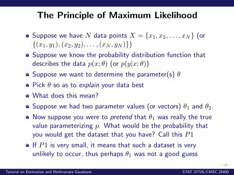
Suppose we have N data points X = x1, x2, . . . , xN (or(x1, y1), (x2, y2), . . . , (xN , yN ))Suppose we know the probability distribution function thatdescribes the data p(x; θ) (or p(y|x; θ))

Suppose we want to determine the parameter(s) θ

Pick θ so as to explain your data best

What does this mean?

Suppose we had two parameter values (or vectors) θ1 and θ2.

Now suppose you were to pretend that θ1 was really the truevalue parameterizing p. What would be the probability thatyou would get the dataset that you have? Call this P1

If P1 is very small, it means that such a dataset is veryunlikely to occur, thus perhaps θ1 was not a good guess



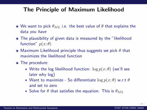
We want to pick θML i.e. the best value of θ that explains thedata you have

The plausibility of given data is measured by the ”likelihoodfunction” p(x; θ)

Maximum Likelihood principle thus suggests we pick θ thatmaximizes the likelihood function

The procedure:

• Write the log likelihood function: log p(x; θ) (we’ll seelater why log)

• Want to maximize - So differentiate log p(x; θ) w.r.t θand set to zero

• Solve for θ that satisfies the equation. This is θML



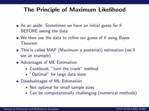
As an aside: Sometimes we have an initial guess for θBEFORE seeing the data

We then use the data to refine our guess of θ using BayesTheorem

This is called MAP (Maximum a posteriori) estimation (we’llsee an example)

Advantages of ML Estimation:

• Cookbook, ”turn the crank” method• ”Optimal” for large data sizes

Disadvantages of ML Estimation

• Not optimal for small sample sizes• Can be computationally challenging (numerical methods)


A Gentle Introduction: Coin Tossing


Problem: estimating bias in coin toss

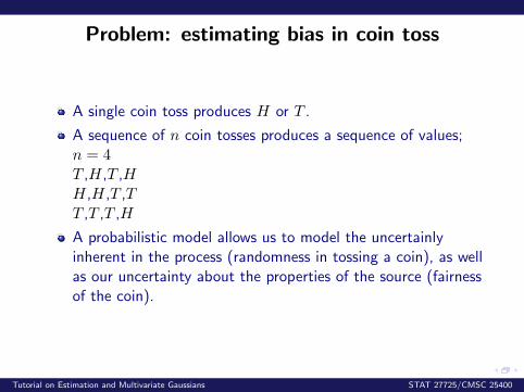
A single coin toss produces H or T .

A sequence of n coin tosses produces a sequence of values;n = 4T ,H,T ,HH,H,T ,TT ,T ,T ,H

A probabilistic model allows us to model the uncertainlyinherent in the process (randomness in tossing a coin), as wellas our uncertainty about the properties of the source (fairnessof the coin).


Probabilistic model

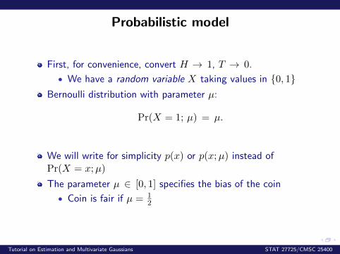
First, for convenience, convert H → 1, T → 0.

• We have a random variable X taking values in 0, 1Bernoulli distribution with parameter µ:

Pr(X = 1; µ) = µ.

We will write for simplicity p(x) or p(x;µ) instead ofPr(X = x;µ)

The parameter µ ∈ [0, 1] specifies the bias of the coin

• Coin is fair if µ = 12


Reminder: probability distributions

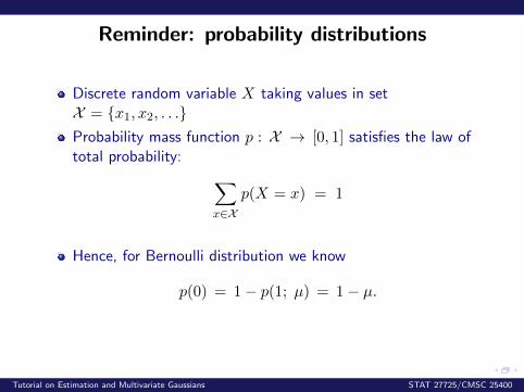
Discrete random variable X taking values in setX = x1, x2, . . .Probability mass function p : X → [0, 1] satisfies the law oftotal probability: ∑

x∈Xp(X = x) = 1

Hence, for Bernoulli distribution we know

p(0) = 1− p(1; µ) = 1− µ.


Sequence probability

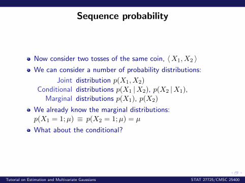
Now consider two tosses of the same coin, 〈X1, X2 〉We can consider a number of probability distributions:

Joint distribution p(X1, X2)Conditional distributions p(X1 |X2), p(X2 |X1),

Marginal distributions p(X1), p(X2)

We already know the marginal distributions:p(X1 = 1;µ) ≡ p(X2 = 1;µ) = µ

What about the conditional?


Sequence probability (contd)

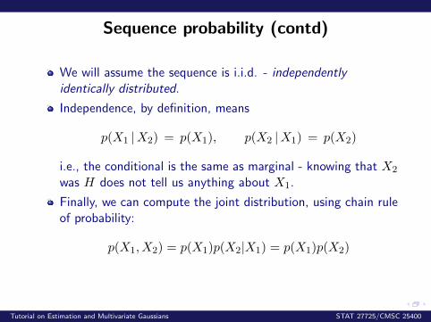
We will assume the sequence is i.i.d. - independentlyidentically distributed.

Independence, by definition, means

p(X1 |X2) = p(X1), p(X2 |X1) = p(X2)

i.e., the conditional is the same as marginal - knowing that X2

was H does not tell us anything about X1.

Finally, we can compute the joint distribution, using chain ruleof probability:

p(X1, X2) = p(X1)p(X2|X1) = p(X1)p(X2)


Sequence probability (contd)

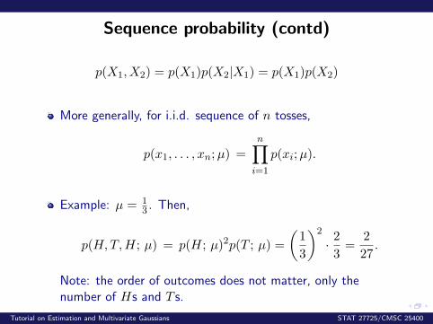
p(X1, X2) = p(X1)p(X2|X1) = p(X1)p(X2)

More generally, for i.i.d. sequence of n tosses,

p(x1, . . . , xn;µ) =

n∏i=1

p(xi;µ).

Example: µ = 13 . Then,

p(H,T,H; µ) = p(H; µ)2p(T ; µ) =

(1

3

)2

· 2

3=

2

27.

Note: the order of outcomes does not matter, only thenumber of Hs and T s.


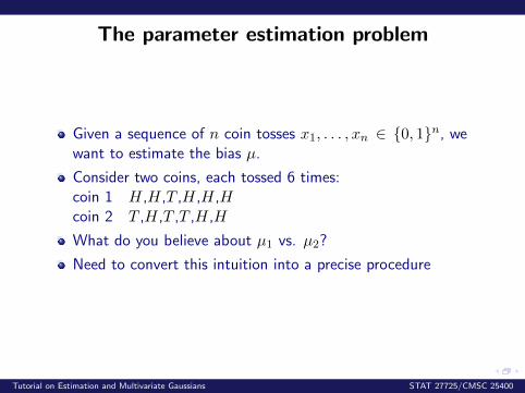
The parameter estimation problem

Given a sequence of n coin tosses x1, . . . , xn ∈ 0, 1n, wewant to estimate the bias µ.

Consider two coins, each tossed 6 times:coin 1 H,H,T ,H,H,Hcoin 2 T ,H,T ,T ,H,H

What do you believe about µ1 vs. µ2?

Need to convert this intuition into a precise procedure


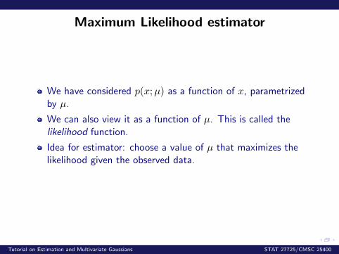
Maximum Likelihood estimator

We have considered p(x;µ) as a function of x, parametrizedby µ.

We can also view it as a function of µ. This is called thelikelihood function.

Idea for estimator: choose a value of µ that maximizes thelikelihood given the observed data.


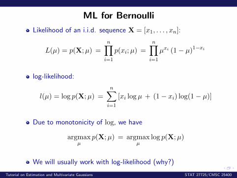
ML for Bernoulli

Likelihood of an i.i.d. sequence X = [x1, . . . , xn]:

L(µ) = p(X;µ) =

n∏i=1

p(xi;µ) =

n∏i=1

µxi (1− µ)1−xi

log-likelihood:

l(µ) = log p(X;µ) =

n∑i=1

[xi logµ + (1− xi) log(1− µ)]

Due to monotonicity of log, we have

argmaxµ

p(X;µ) = argmaxµ

log p(X;µ)

We will usually work with log-likelihood (why?)


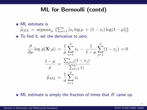
ML for Bernoulli (contd)

ML estimate isµML = argmaxµ

∑ni=1 [xi logµ + (1− xi) log(1− µ)]

To find it, set the derivative to zero:

∂

∂µlog p(X;µ) =

1

µ

n∑i=1

xi −1

1− µn∑j=1

(1− xj) = 0

1− µµ

=

∑nj=1(1− xj)∑n

i=1 xi

µML =1

n

n∑i=1

xi

ML estimate is simply the fraction of times that H came up.


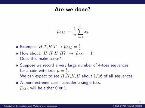
Are we done?

µML =1

n

n∑i=1

xi

Example: H,T ,H,T → µML = 12

How about: H H H H? → µML = 1Does this make sense?

Suppose we record a very large number of 4-toss sequencesfor a coin with true µ = 1

2 .We can expect to see H,H,H,H about 1/16 of all sequences!

A more extreme case: consider a single toss.µML will be either 0 or 1.


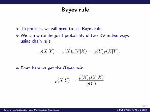
Bayes rule

To proceed, we will need to use Bayes rule

We can write the joint probability of two RV in two ways,using chain rule:

p(X,Y ) = p(X)p(Y |X) = p(Y )p(X|Y ).

From here we get the Bayes rule:

p(X|Y ) =p(X)p(Y |X)

p(Y )


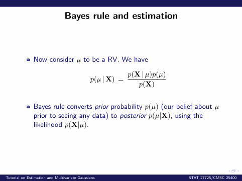
Bayes rule and estimation

Now consider µ to be a RV. We have

p(µ |X) =p(X |µ)p(µ)

p(X)

Bayes rule converts prior probability p(µ) (our belief about µprior to seeing any data) to posterior p(µ|X), using thelikelihood p(X|µ).


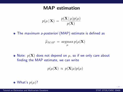
MAP estimation

p(µ |X) =p(X |µ)p(µ)

p(X)

The maximum a-posteriori (MAP) estimate is defined as

µMAP = argmaxµ

p(µ|X)

Note: p(X) does not depend on µ, so if we only care aboutfinding the MAP estimate, we can write

p(µ|X) ∝ p(X|µ)p(µ)

What’s p(µ)?


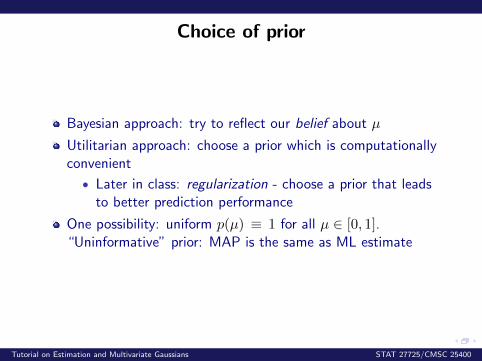
Choice of prior

Bayesian approach: try to reflect our belief about µ

Utilitarian approach: choose a prior which is computationallyconvenient

• Later in class: regularization - choose a prior that leadsto better prediction performance

One possibility: uniform p(µ) ≡ 1 for all µ ∈ [0, 1].“Uninformative” prior: MAP is the same as ML estimate


Constrained Optimization: A Multinomial Likelihood


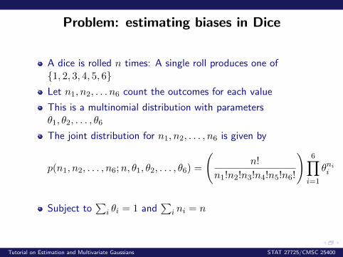
Problem: estimating biases in Dice

A dice is rolled n times: A single roll produces one of1, 2, 3, 4, 5, 6Let n1, n2, . . . n6 count the outcomes for each value

This is a multinomial distribution with parametersθ1, θ2, . . . , θ6

The joint distribution for n1, n2, . . . , n6 is given by

p(n1, n2, . . . , n6;n, θ1, θ2, . . . , θ6) =

(n!

n1!n2!n3!n4!n5!n6!

)6∏i=1

θnii

Subject to∑

i θi = 1 and∑

i ni = n


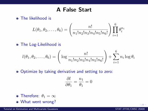
A False Start

The likelihood is

L(θ1, θ2, . . . , θ6) =

(n!

n1!n2!n3!n4!n5!n6!

)6∏i=1

θnii

The Log-Likelihood is

l(θ1, θ2, . . . , θ6) =

(log

n!

n1!n2!n3!n4!n5!n6!

)+

6∑i=1

ni log θi

Optimize by taking derivative and setting to zero:

∂l

∂θ1=n1θ1

= 0

Therefore: θ1 =∞What went wrong?


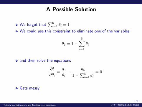
A Possible Solution

We forgot that∑6

i=1 θi = 1

We could use this constraint to eliminate one of the variables:

θ6 = 1−5∑i=1

θi

and then solve the equations

∂l

∂θi=n1θi− n6

1−∑5i=1 θi

= 0

Gets messy


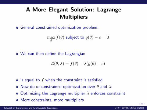
A More Elegant Solution: LagrangeMultipliers

General constrained optimization problem:

maxθf(θ) subject to g(θ)− c = 0

We can then define the Lagrangian

L(θ, λ) = f(θ)− λ(g(θ)− c)

Is equal to f when the constraint is satisfied

Now do unconstrained optimization over θ and λ:

Optimizing the Lagrange multiplier λ enforces constraint

More constraints, more multipliers


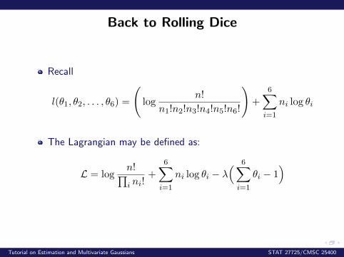
Back to Rolling Dice

Recall

l(θ1, θ2, . . . , θ6) =

(log

n!

n1!n2!n3!n4!n5!n6!

)+

6∑i=1

ni log θi

The Lagrangian may be defined as:

L = logn!∏i ni!

+

6∑i=1

ni log θi − λ( 6∑i=1

θi − 1)


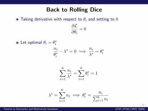
Back to Rolling Dice

Taking derivative with respect to θi and setting to 0

∂L∂θi

= 0

Let optimal θi = θ∗iniθ∗i− λ∗ = 0 =⇒ ni

λ∗= θ∗i

6∑i=1

niλ∗

=

6∑i=1

θ∗i = 1

λ∗ =6∑i=1

ni =⇒ θ∗i =ni∑6i=1 ni


Multivariate Gaussians


Quick Review: Discrete/Continuous RandomVariables

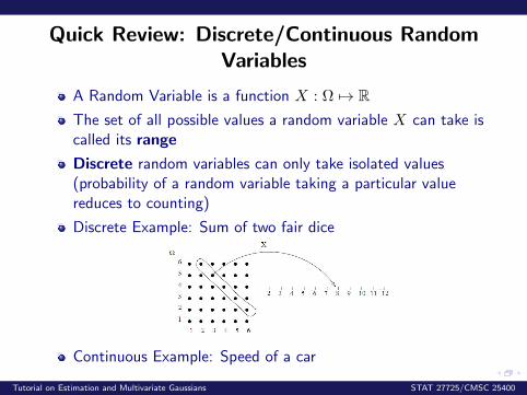
A Random Variable is a function X : Ω 7→ RThe set of all possible values a random variable X can take iscalled its range

Discrete random variables can only take isolated values(probability of a random variable taking a particular valuereduces to counting)

Discrete Example: Sum of two fair dice

Continuous Example: Speed of a car


Discrete Distributions

Assume X is a discrete random variable. We would like tospecify probabilities of events X = xIf we can specify the probabilities involving X, we can saythat we have specified the probability distribution of X

For a countable set of values x1, x2, . . . xn, we haveP(X = xi) > 0, i = 1, 2, . . . , n and

∑i P(X = xi) = 1

We can then define the probability mass function f of X byf(X) = P(X = x)

Sometimes write as fX


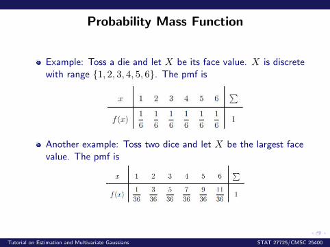
Probability Mass Function

Example: Toss a die and let X be its face value. X is discretewith range 1, 2, 3, 4, 5, 6. The pmf is

Another example: Toss two dice and let X be the largest facevalue. The pmf is


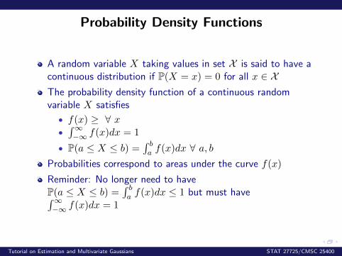
Probability Density Functions

A random variable X taking values in set X is said to have acontinuous distribution if P(X = x) = 0 for all x ∈ XThe probability density function of a continuous randomvariable X satisfies

• f(x) ≥ ∀ x•∫∞−∞ f(x)dx = 1

• P(a ≤ X ≤ b) =∫ ba f(x)dx ∀ a, b

Probabilities correspond to areas under the curve f(x)

Reminder: No longer need to haveP(a ≤ X ≤ b) =

∫ ba f(x)dx ≤ 1 but must have∫∞

−∞ f(x)dx = 1


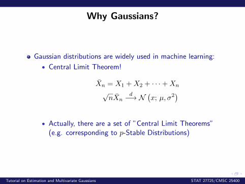
Why Gaussians?

Gaussian distributions are widely used in machine learning:

• Central Limit Theorem!

Xn = X1 +X2 + · · ·+Xn

√nXn

d−→ N(x; µ, σ2

)• Actually, there are a set of ”Central Limit Theorems”

(e.g. corresponding to p-Stable Distributions)


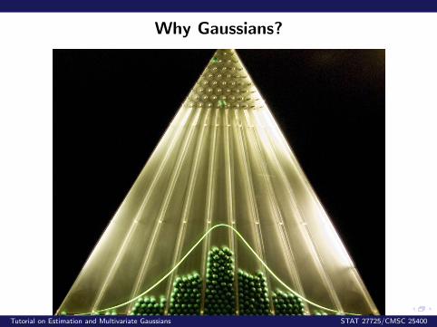
Why Gaussians?


Why Gaussians?

Gaussian distributions are widely used in machine learning:

• Central Limit Theorem!• Gaussians are convenient computationally;• Mixtures of Gaussians (just covered in class) are

sufficient to approximate a wide range of distributions;• Closely related to squared loss (have seen earlier in class),

an important error measure in statistics.


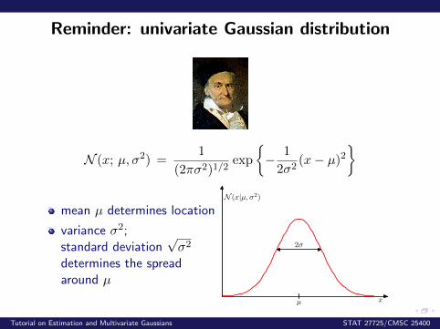
Reminder: univariate Gaussian distribution

N (x; µ, σ2) =1

(2πσ2)1/2exp

− 1

2σ2(x− µ)2

mean µ determines location

variance σ2;standard deviation

√σ2

determines the spreadaround µ

N (x|µ, σ2)

x

2σ

µ


Moments

Reminder: expectation of a RV x is E [x] ,∫xp(x)dx, so

E [x] =

∫ ∞−∞

xN (x;µ, σ2)dx = µ

Variance of x is varx , E[(x− E [x])2

], and

varx =

∫ ∞−∞

(x− µ)2N (x;µ, σ2)dx = σ2


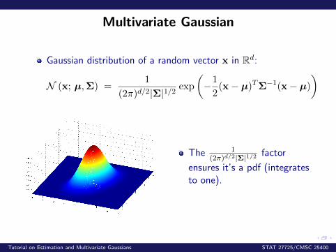
Multivariate Gaussian

Gaussian distribution of a random vector x in Rd:

N (x; µ,Σ) =1

(2π)d/2|Σ|1/2 exp

(−1

2(x− µ)TΣ−1(x− µ)

)

The 1(2π)d/2|Σ|1/2 factor

ensures it’s a pdf (integratesto one).


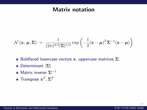
Matrix notation

N (x; µ,Σ) =1

(2π)d/2|Σ|1/2 exp

(−1

2(x− µ)TΣ−1(x− µ)

)

Boldfaced lowercase vectors x, uppercase matrices Σ.

Determinant |Σ|Matrix inverse Σ−1

Transpose xT ,ΣT


Mean of the Gaussian

By definition,

E [x] =

∫ ∞−∞

. . .

∫ ∞−∞

xN (x;µ,Σ)dx1 . . . dxd

Solving this we indeed get

E [x] = µ


Covariance

Variance of a RV x with mean µ: σ2x = E[(x− µ)2

]Generalization to two variables: covariance

Covx1,x2 , E [(x1 − µ1)(x2 − µ2)]

Measures how the two variables deviate together from theirmeans (“co-vary”).

Note: Covx,x ≡ var(x) = σ2x


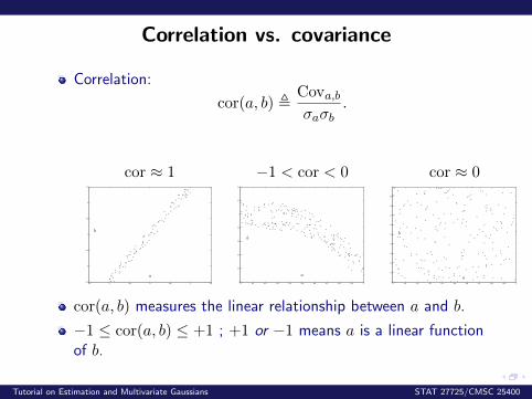
Correlation vs. covariance

Correlation:

cor(a, b) ,Cova,bσaσb

.

cor ≈ 1 −1 < cor < 0 cor ≈ 0

−1.5 −1 −0.5 0 0.5 1 1.5−1.5

−1

−0.5

0

0.5

1

1.5

a

b

0 0.1 0.2 0.3 0.4 0.5 0.6 0.7 0.8 0.9 10

0.2

0.4

0.6

0.8

1

1.2

1.4

a

b

0 0.1 0.2 0.3 0.4 0.5 0.6 0.7 0.8 0.9 10

0.1

0.2

0.3

0.4

0.5

0.6

0.7

0.8

0.9

1

a

b

cor(a, b) measures the linear relationship between a and b.

−1 ≤ cor(a, b) ≤ +1 ; +1 or −1 means a is a linear functionof b.


Covariance matrix

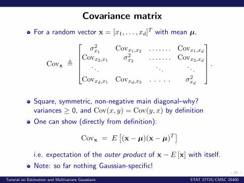
For a random vector x = [x1, . . . , xd]T with mean µ,

Covx ,

σ2x1 Covx1,x2 . . . . . . . Covx1,xd

Covx2,x1 σ2x2 . . . . . . . Covx2,xd. . .

. . .. . .

Covxd,x1 Covxd,x2 . . . . . σ2xd

.

Square, symmetric, non-negative main diagonal–why?variances ≥ 0, and Cov(x, y) = Cov(y, x) by definition

One can show (directly from definition):

Covx = E[(x− µ)(x− µ)T

]i.e. expectation of the outer product of x− E [x] with itself.

Note: so far nothing Gaussian-specific!


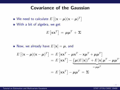
Covariance of the Gaussian

We need to calculate E[(x− µ)(x− µ)T

]With a bit of algebra, we get

E[xxT

]= µµT + Σ

Now, we already have E [x] = µ, and

E[(x− µ)(x− µ)T

]= E

[xxT − µxT − xµT + µµT

]= E

[xxT

]−µ(E [x])T + E [x]µT − µµT

︸︷︷︸=µµT

= E[xxT

]− µµT = Σ


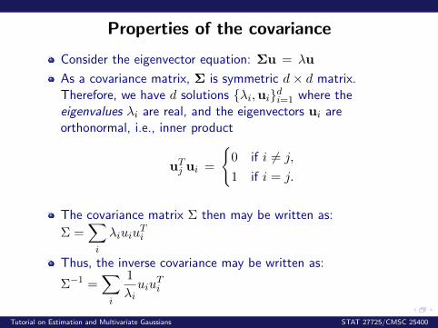
Properties of the covariance

Consider the eigenvector equation: Σu = λu

As a covariance matrix, Σ is symmetric d× d matrix.Therefore, we have d solutions λi,uidi=1 where theeigenvalues λi are real, and the eigenvectors ui areorthonormal, i.e., inner product

uTj ui =

0 if i 6= j,

1 if i = j.

The covariance matrix Σ then may be written as:

Σ =∑i

λiuiuTi

Thus, the inverse covariance may be written as:

Σ−1 =∑i

1

λiuiu

Ti


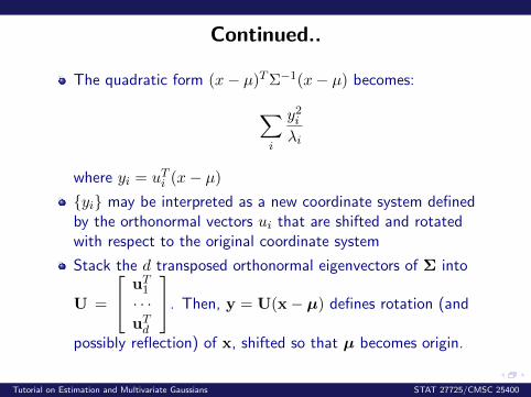
Continued..

The quadratic form (x− µ)TΣ−1(x− µ) becomes:

∑i

y2iλi

where yi = uTi (x− µ)

yi may be interpreted as a new coordinate system definedby the orthonormal vectors ui that are shifted and rotatedwith respect to the original coordinate system

Stack the d transposed orthonormal eigenvectors of Σ into

U =

uT1· · ·uTd

. Then, y = U(x− µ) defines rotation (and

possibly reflection) of x, shifted so that µ becomes origin.


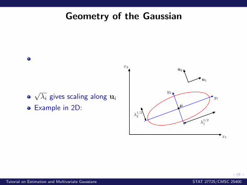
Geometry of the Gaussian

√λi gives scaling along ui

Example in 2D:

x1

x2

λ1/21

λ1/22

y1

y2

u1

u2

µ


Geometry Continued ...

The determinant of the covariance matrix may be written as

the product of its eigenvalues i.e. |Σ| 12 =∏j λ

12j

Thus, in the yi coordinate system, the Gaussian distributiontakes the form:

p(y) =∏j

1

(2πλj)12

exp

(−y2j2λj

)

which is the product of d independent univariate Gaussians

The eigenvectors thus define a new set of shifted and rotatedcoordinates w.r.t which the joint probability distributionfactorizes into a product of independent distributions


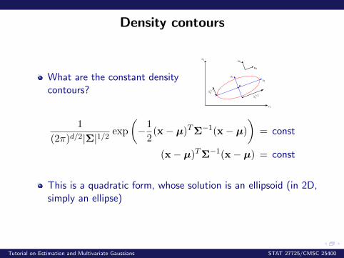
Density contours

What are the constant densitycontours?

x1

x2

λ1/21

λ1/22

y1

y2

u1

u2

µ

1

(2π)d/2|Σ|1/2 exp

(−1

2(x− µ)TΣ−1(x− µ)

)= const

(x− µ)TΣ−1(x− µ) = const

This is a quadratic form, whose solution is an ellipsoid (in 2D,simply an ellipse)


Density Contours are Ellipsoids

We saw that: (x− µ)TΣ−1(x− µ) = const2

Recall that Σ−1 =∑i

1

λiuiu

Ti

Thus we have: ∑i

y2iλi

= const2

where yi = uTi (x− µ)

Recall the expression for an ellipse in 2D:(xa

)2+(yb

)2= 1


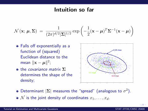
Intuition so far

N (x; µ,Σ) =1

(2π)d/2|Σ|1/2 exp

(−1

2(x− µ)TΣ−1(x− µ)

)

Falls off exponentially as afunction of (squared)Euclidean distance to themean ‖x− µ‖2;

the covariance matrix Σdetermines the shape of thedensity;

−4 −3 −2 −1 0 1 2 3 4−4

−3

−2

−1

0

1

2

3

4

0.05 max

0.5 max

0.9 max

Determinant |Σ| measures the “spread” (analogous to σ2).

N is the joint density of coordinates x1, . . . , xd.


Linear functions of a Gaussian RV

For any RV x, and for any A and b,

E [Ax + b] = AE [x]+b, Cov(Ax+b) = A Cov(x)AT .

Let x ∼ N (·; µ,Σ); then p(z) = N(z; Aµ + b, AΣAT

).

Consider a row vector aT that “selects” a single componentfrom x, i.e., ak = 1 and aj = 0 if j 6= k. Then, z = aTx issimply the coordinate xk.

We have: E [z] = aTµ = µk, and Cov(z) = var(z) = Σk,k.i.e., marginal of a Gaussian is also a Gaussian


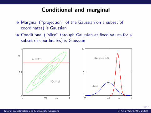
Conditional and marginal

Marginal (“projection” of the Gaussian on a subset ofcoordinates) is Gaussian

Conditional (“slice” through Gaussian at fixed values for asubset of coordinates) is Gaussian

xa

xb = 0.7

xb

p(xa, xb)

0 0.5 10

0.5

1

xa

p(xa)

p(xa|xb = 0.7)

0 0.5 10

5

10


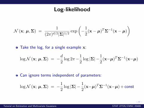
Log-likelihood

N (x; µ,Σ) =1

(2π)d/2|Σ|1/2 exp

(−1

2(x− µ)TΣ−1(x− µ)

)

Take the log, for a single example x:

logN (x; µ,Σ) = −d2

log 2π−1

2log |Σ| −1

2(x−µ)TΣ−1(x−µ)

Can ignore terms independent of parameters:

logN (x; µ,Σ) = −1

2log |Σ| − 1

2(x−µ)TΣ−1(x−µ) + const


Log-likelihood (contd)

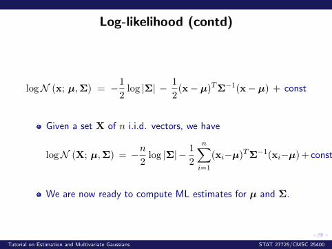
logN (x; µ,Σ) = −1

2log |Σ| − 1

2(x− µ)TΣ−1(x− µ) + const

Given a set X of n i.i.d. vectors, we have

logN (X; µ,Σ) = −n2

log |Σ| − 1

2

n∑i=1

(xi−µ)TΣ−1(xi−µ) + const

We are now ready to compute ML estimates for µ and Σ.


ML for parameters

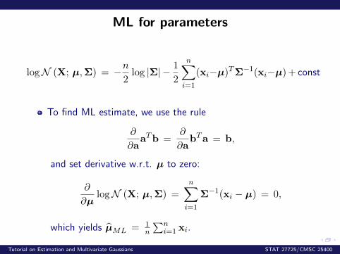
logN (X; µ,Σ) = −n2

log |Σ| − 1

2

n∑i=1

(xi−µ)TΣ−1(xi−µ) + const

To find ML estimate, we use the rule

∂

∂aaTb =

∂

∂abTa = b,

and set derivative w.r.t. µ to zero:

∂

∂µlogN (X; µ,Σ) =

n∑i=1

Σ−1(xi − µ) = 0,

which yields µML = 1n

∑ni=1 xi.


ML for parameters (contd)

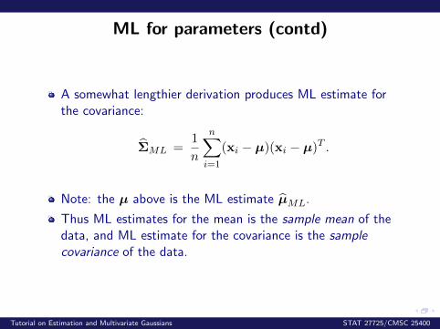
A somewhat lengthier derivation produces ML estimate forthe covariance:

ΣML =1

n

n∑i=1

(xi − µ)(xi − µ)T .

Note: the µ above is the ML estimate µML.

Thus ML estimates for the mean is the sample mean of thedata, and ML estimate for the covariance is the samplecovariance of the data.


Mixture Models and Expected Log Likelihood


Mixture Models

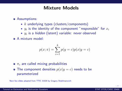
Assumptions:

• k underlying types (clusters/components)• yi is the identity of the component ”responsible” for xi• yi is a hidden (latent) variable: never observed

A mixture model:

p(x;π) =

k∑c=1

p(y = c)p(x|y = c)

πc are called mixing probabilities

The component densities p(x|y = c) needs to beparameterized

Next few slides adapted from TTIC 31020 by Gregory Shakhnarovich


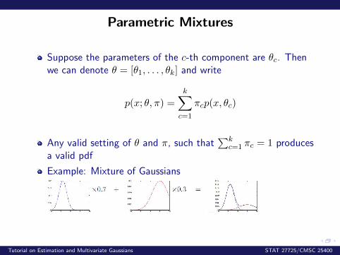
Parametric Mixtures

Suppose the parameters of the c-th component are θc. Thenwe can denote θ = [θ1, . . . , θk] and write

p(x; θ, π) =

k∑c=1

πcp(x, θc)

Any valid setting of θ and π, such that∑k

c=1 πc = 1 producesa valid pdf

Example: Mixture of Gaussians


Generative Model for a Mixture

The generative process with a k-component mixture:• The parameters θc for each component are fixed• Draw yi ∼ [π1, . . . , πk]• Given yi, draw xi ∼ p(x|yi; θyi)

The entire generative model for x and y

p(x, y; θ, π) = p(y;π)p(x|y; θy)

What does this mean? Any data point xi could have beengenerated in k ways

If the c-th component is Gaussian i.e.p(x|y = c) = N (x;µc,Σc)

p(x; θ, π) =

k∑c=1

πcN (x;µc,Σc)

where θ = [µ1, . . . , µk,Σ1, . . . ,Σk]


Likelihood of a Mixture Model

Usual Idea: Estimate set of parameters that maximizelikelihood given observed data

The log-likelihood of π, θ for X = x1, . . . , xN:

log p(X;π, θ) =

N∑i=1

log

k∑c=1

πcN (xi;µc,Σc)

No closed form solution because of sum inside log

How will we estimate parameters?


Scenario 1: Known Labels. Mixture DensityEstimation

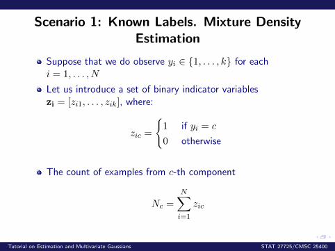
Suppose that we do observe yi ∈ 1, . . . , k for eachi = 1, . . . , N

Let us introduce a set of binary indicator variableszi = [zi1, . . . , zik], where:

zic =

1 if yi = c

0 otherwise

The count of examples from c-th component

Nc =N∑i=1

zic


Scenario 1: Known Labels. Mixture DensityEstimation

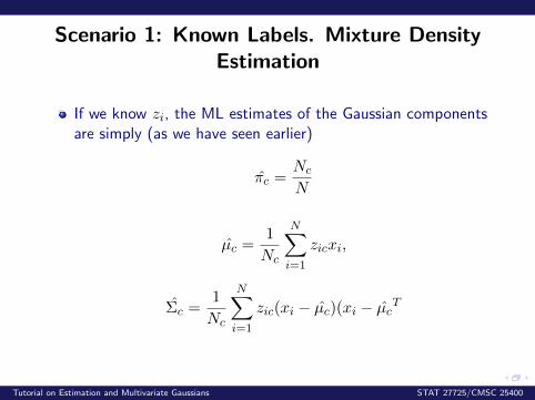
If we know zi, the ML estimates of the Gaussian componentsare simply (as we have seen earlier)

πc =Nc

N

µc =1

Nc

N∑i=1

zicxi,

Σc =1

Nc

N∑i=1

zic(xi − µc)(xi − µcT


Scenario 2: Credit Assignment

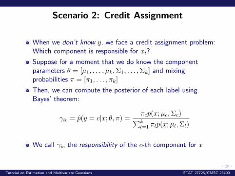
When we don’t know y, we face a credit assignment problem:Which component is responsible for xi?

Suppose for a moment that we do know the componentparameters θ = [µ1, . . . , µk,Σ1, . . . ,Σk] and mixingprobabilities π = [π1, . . . , πk]

Then, we can compute the posterior of each label usingBayes’ theorem:

γic = p(y = c|x; θ, π) =πcp(x;µc,Σc)∑kl=1 πlp(x;µl,Σl)

We call γic the responsibility of the c-th component for x


Expected Likelihood

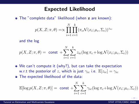
The ”complete data” likelihood (when z are known):

p(X,Z;π, θ) =∝N∏i=1

k∏c=1

(πcN (xi;µc,Σc))zic

and the log

p(X,Z;π, θ) = const +

N∑i=1

k∑c=1

zic(log πc+logN (xi;µc,Σc))

We can’t compute it (why?), but can take the expectationw.r.t the posterior of z, which is just γic i.e. E[zic] = γicThe expected likelihood of the data:

E[log p(X,Z;π, θ)] = const +

N∑i=1

k∑c=1

γic(log πc+logN (xi;µc,Σc))


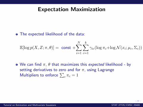
Expectation Maximization

The expected likelihood of the data:

E[log p(X,Z;π, θ)] = const +

N∑i=1

k∑c=1

γic(log πc+logN (xi;µc,Σc))

We can find π, θ that maximizes this expected likelihood - bysetting derivatives to zero and for π, using LagrangeMultipliers to enforce

∑c πc = 1


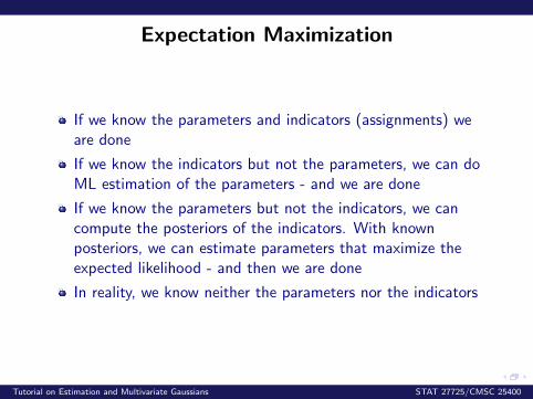
Expectation Maximization

If we know the parameters and indicators (assignments) weare done

If we know the indicators but not the parameters, we can doML estimation of the parameters - and we are done

If we know the parameters but not the indicators, we cancompute the posteriors of the indicators. With knownposteriors, we can estimate parameters that maximize theexpected likelihood - and then we are done

In reality, we know neither the parameters nor the indicators


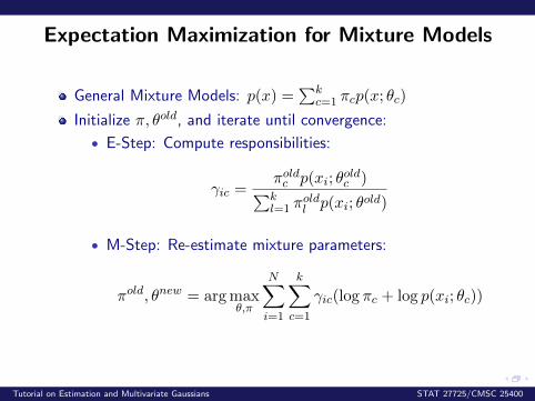
Expectation Maximization for Mixture Models

General Mixture Models: p(x) =∑k

c=1 πcp(x; θc)

Initialize π, θold, and iterate until convergence:

• E-Step: Compute responsibilities:

γic =πoldc p(xi; θ

oldc )∑k

l=1 πoldl p(xi; θold)

• M-Step: Re-estimate mixture parameters:

πold, θnew = arg maxθ,π

N∑i=1

k∑c=1

γic(log πc + log p(xi; θc))


Documents

Tutorial on Estimation and Multivariate Gaussiansttic.uchicago.edu/~shubhendu/Slides/Estimation.pdf · Tutorial on Estimation and Multivariate Gaussians ... Maximum Likelihood Estimation