TUTORIAL ON DIGITAL MODULATIONS Part 1: … communication systems.pdf · TUTORIAL ON DIGITAL MODULATIONS Part 1: Introduction to digital communication systems. Fundamental quantities

TUTORIAL ON DIGITAL MODULATIONSTUTORIAL ON DIGITAL MODULATIONS

Part 1: Introduction to digital communication Part 1: Introduction to digital communication systems. Fundamental quantities.systems. Fundamental quantities.

[[20112011--1010--26]26]

1

Roberto Roberto GarelloGarello, Politecnico di Torino, Politecnico di Torino

Free download (Free download (forfor personal personal useuse onlyonly) at: ) at: www.tlc.polito.it/www.tlc.polito.it/garellogarello

Author:

Roberto GARELLO, Ph.D.

Associate Professor in Communication Engineering

Dipartimento di Elettronica

Politecnico di Torino, Italy

R. Garello. “Tutorial on digital modulations - Part 1” 2

Politecnico di Torino, Italy

email: [email protected]

web: www.tlc.polito.it/garello

Part 1: Part 1:

Introduction to digital communication systems.Introduction to digital communication systems.

Fundamental quantities Fundamental quantities

Summary:


−Introduction to digital communication systems.

−The 5 Fundamental quantities: Bit rate, Bandwidth,

Power, Error rate, Complexity.

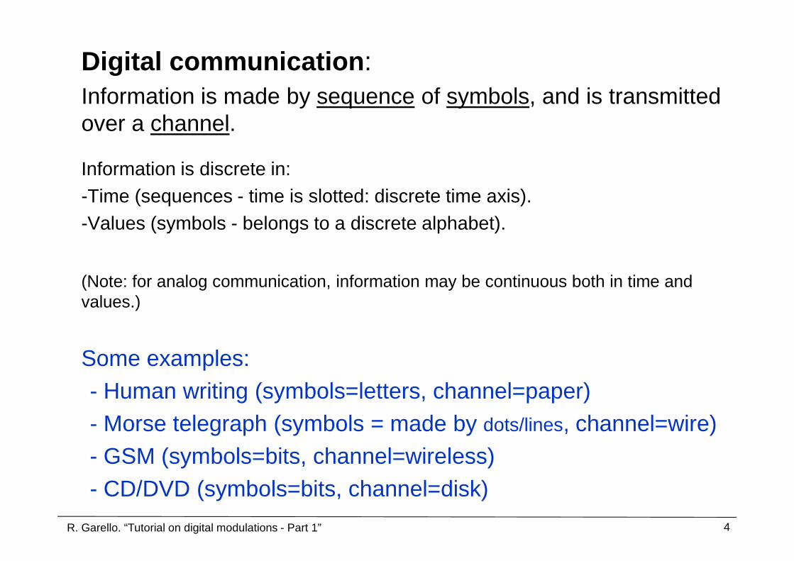
Digital communication : Information is made by sequence of symbols, and is transmitted over a channel.

Information is discrete in:-Time (sequences - time is slotted: discrete time axis).-Values (symbols - belongs to a discrete alphabet).

(Note: for analog communication, information may be continuous both in time and


(Note: for analog communication, information may be continuous both in time and values.)

Some examples:- Human writing (symbols=letters, channel=paper)- Morse telegraph (symbols = made by dots/lines, channel=wire)- GSM (symbols=bits, channel=wireless)- CD/DVD (symbols=bits, channel=disk)

Digital communication systems considered in this tutorial.

We focus on systems characterized by these two properties:

1. Symbols = bits� Discrete alphabet = Binary alphabet {0,1} � Information = binary sequences


Note: Even when analog information must be transmitted (voice, etc.), we suppose that by sampling and quantization (+source coding), it has already been converted into binary information sequences.

2. Transmission channel = wireless or wired channel (no disks or other media)

Wireless channel:

Transmitter and receiver are connected by two antennas


Transmitter and receiver are connected by two antennas

Wired channel:

Transmitter and receiver are connected by a cable

Digital communication systems considered in this tutorial.

=

binary information sequences are transmitted over a wireless or wired channel


The system (transmitter TX+receiver RX)

exists to transmit binary information sequence

over the channel

Examples of digital communication systemsExamples of digital communication systems

� Copperline modems (V90 / xDSL)

� Ethernet

� Powerline communication

� Optical Fiber modems

wired


� Optical Fiber modems

Examples of digital communication systemsExamples of digital communication systems

�Transmission from space: Space missions, satellite communication, GNSS (GPS, Galileo, Glonass, …)

� Digital Television: DVB (T,S,H)

� Cellular systems: GSM/UMTS/LTE wireless


� Long range systems: digital radio links

�Medium range systems: Wi-Fi, WiMAX

�Short range systems: Wireless sensor networks Zigbee, Bluetooth, Ultrawideband, RFID

wireless

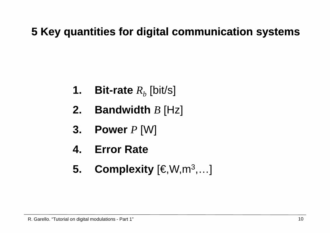
5 Key quantities for digital communication systems 5 Key quantities for digital communication systems

1. Bit-rate Rb [bit/s]

2. Bandwidth B [Hz]


3. Power P [W]

4. Error Rate

5. Complexity [€,W,m3,…]

source TX RXCHANNEL

Tu ( )s t ( )r t Ru

Transmitter Receiver


Transmitted binary information sequences

Transmitted signal (waveform)

Received signal (waveform)

Received binary information sequences

Tu

( )s t

( )r t

Ru

Binary information sequences are characterized by their “speed”

� Bit-rate = number of bits transmitted in a second [bit/s, bps]

1 1 -- BitBit--rate rate Rb [bps]


source TX RXCHANNEL

Tu ( )s t ( )r t Ru

bR bR

Examples of bitExamples of bit--rate:rate:

� xDSL: up to tens of Mbps

� Ethernet: up to 100 Gbps

� Optical Fiber modems: up to Terabps

� GSM: 9600 bps/UMTS: some Mbps/LTE: hundreds of Mbps


� GSM: 9600 bps/UMTS: some Mbps/LTE: hundreds of Mbps

� DVB (S,T): tens of Mbps

� Wi-Fi: tens/hundreds of Mbps, WiMAX: hundreds of Mbps

� GPS/Galileo: bps

A KEY ASPECT. A binary information sequences is a sequence of bits.

To be transmitted over a wireless or wired channel, it must be transformed into a physical waveform: the transmitted signal s(t)

[a voltage evolving in time]

2 2 –– Bandwidth Bandwidth B [Hz]


[a voltage evolving in time]

TX CHANNEL

Tu ( )s t

01100...u =

0 2 4 6 8

t/Tb

0 2 4 6 8

t/Tb

Simplest example of association uT � s(t) (bipolar NRZ):

V

0 t

-V

Tb

1 1 1 1Tu =( )s t

0 0 0


Bit 1: voltage +V for Tb = 1/Rb s

Bit 0: voltage –V for Tb = 1/Rb s

V

0 t

-V

Tb

s(t) is characterized by a given behavior on the frequency axis � power spectral density (spectrum) Gs(f)

[distribution of the power on the frequency axis, will be fully addressed later]

binary information sequences

transmitted signal s(t)

+∞


source TX RXCHANNEL

Tu ( )s t ( )r t Ru

( )sG f

power ( )s sP G f df+∞

−∞

= ∫

V

0 t

-V

Tb

0 0.5 1 1.5 2 2.5 3 f bT

G (f)x

-0.5-1-1.5-2-2.5-3

( )sG f

( )s t

Power spectral density (frequency behavior)

NRZ example Transmitted waveform (time behavior)


2sin( )

( )( )

bs

b

fTG f

fT

παπ

=

0 0.5 1 1.5 2 2.5 3 f bT

G (f)x

-0.5-1-1.5-2-2.5-3

source TX RXCHANNEL

Tu ( )s t ( )r t Ru

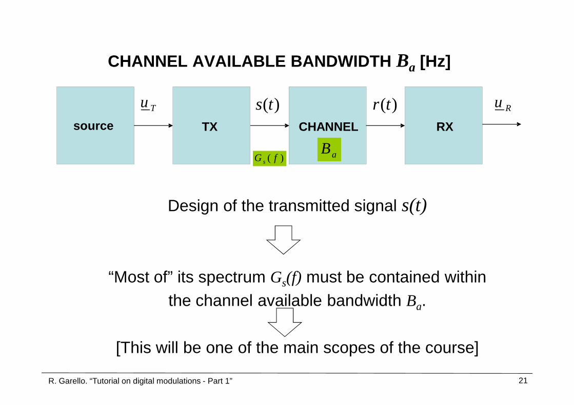
CHANNEL AVAILABLE BANDWIDTH Ba [Hz]

Any channel is characterized by an available bandwidth B :

aB( )sG f


Any channel is characterized by an available bandwidth Ba:

“most of” the spectrum Gs(f) must be contained within Ba.

Two typical reasons:

Out of Ba , channel frequency response is very bad. Typical for wired channels : the transmission medium (the cable) is completely dedicated to the communication system: in line of principle we could use all the frequencies, but we choose to limit them at a given maximum frequency because at higher frequencies the cable response is too bad (cables have a low-


frequencies the cable response is too bad (cables have a low-pass frequency response).

Out of Ba , other systems are transmitting on adjacent bands. Typical for wireless channels : many users sharing the same transmission medium (the air). Each system has a pre-assigned limited available band and it cannot disturb the systems transmitting on the other bands.

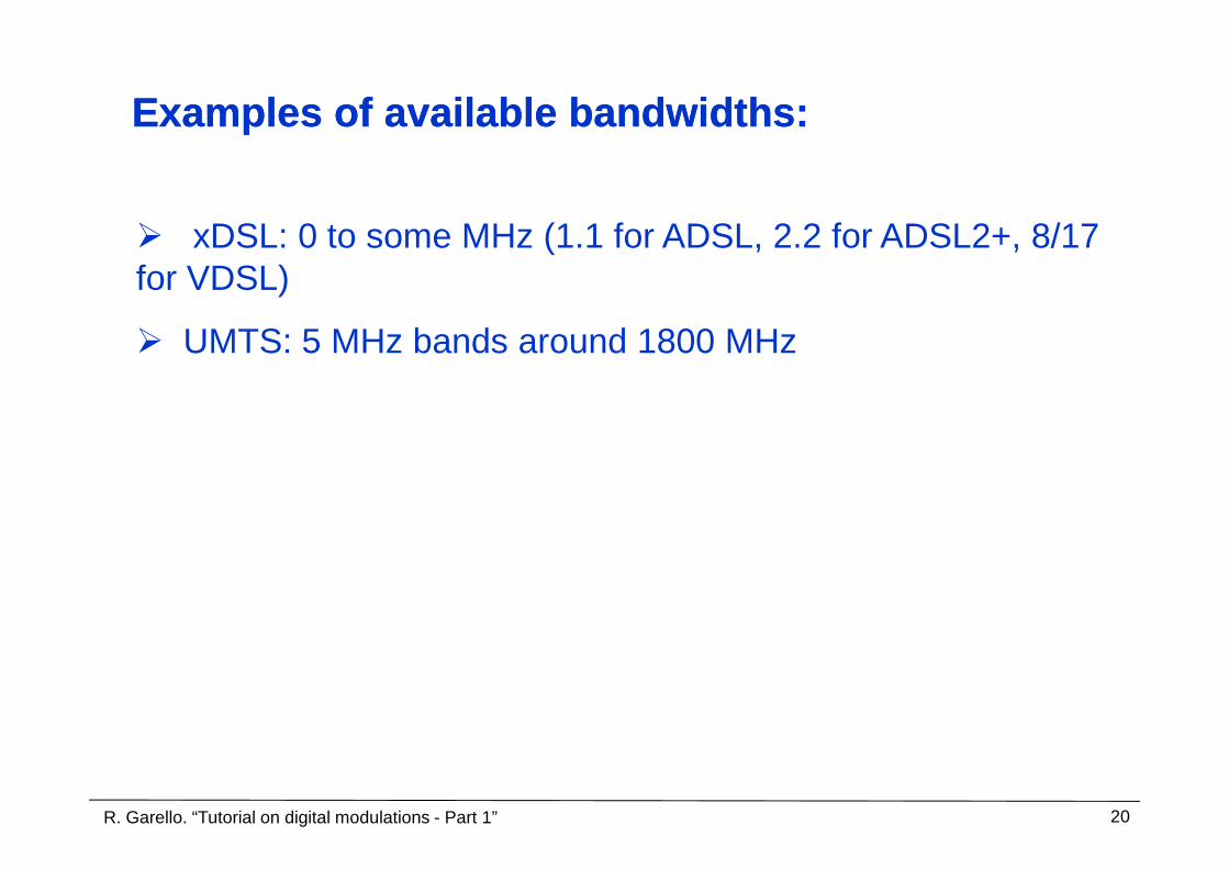
Examples of available bandwidths:Examples of available bandwidths:

� xDSL: 0 to some MHz (1.1 for ADSL, 2.2 for ADSL2+, 8/17 for VDSL)

� UMTS: 5 MHz bands around 1800 MHz


source TX RXCHANNEL

Tu ( )s t ( )r t Ru

Design of the transmitted signal s(t)

CHANNEL AVAILABLE BANDWIDTH Ba [Hz]

aB( )sG f


Design of the transmitted signal s(t)

“Most of” its spectrum Gs(f) must be contained withinthe channel available bandwidth Ba.

[This will be one of the main scopes of the course]

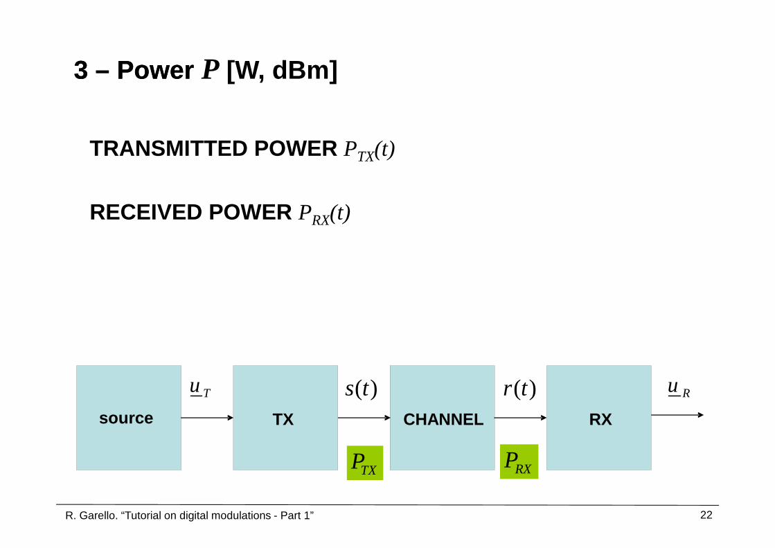
TRANSMITTED POWER PTX(t)

RECEIVED POWER PRX(t)

3 3 –– Power Power P [W, dBm]


source TX RXCHANNEL

Tu ( )s t ( )r t Ru

TXP RXP

Transmitted power is limited by a number of factorsTransmitted power is limited by a number of factors

• Avoid interference with adjacent channels

• EM compatibility


• Max power transmitted by a device working at that frequency

• Total power (battery)

• Linearity constraints

Received power is connected to transmitted power Received power is connected to transmitted power (distance, frequency, environment,system,….)(distance, frequency, environment,system,….)

Example: Line of Sight wireless link


24

T RR T

G GP P

dπλ

=

CHANNEL

( )s t ( )r t

TXP RXP

Received power is connected to transmitted power Received power is connected to transmitted power (distance, frequency, (distance, frequency, environment,systemenvironment,system,….),….)

Example: copperline frequency response

TR

PP

A=

CHANNEL

( )s t ( )r t

TXP RXP90

10020 m50 m

100 m200 m500 m


TX RX

10

20

30

40

50

60

70

80

1e+01 1e+02 1e+03 1e+04 1e+05

A [d

B]

f [kHz]

200 m500 m

1000 m2000 m5000 m

attenuation increases with

frequency and line length

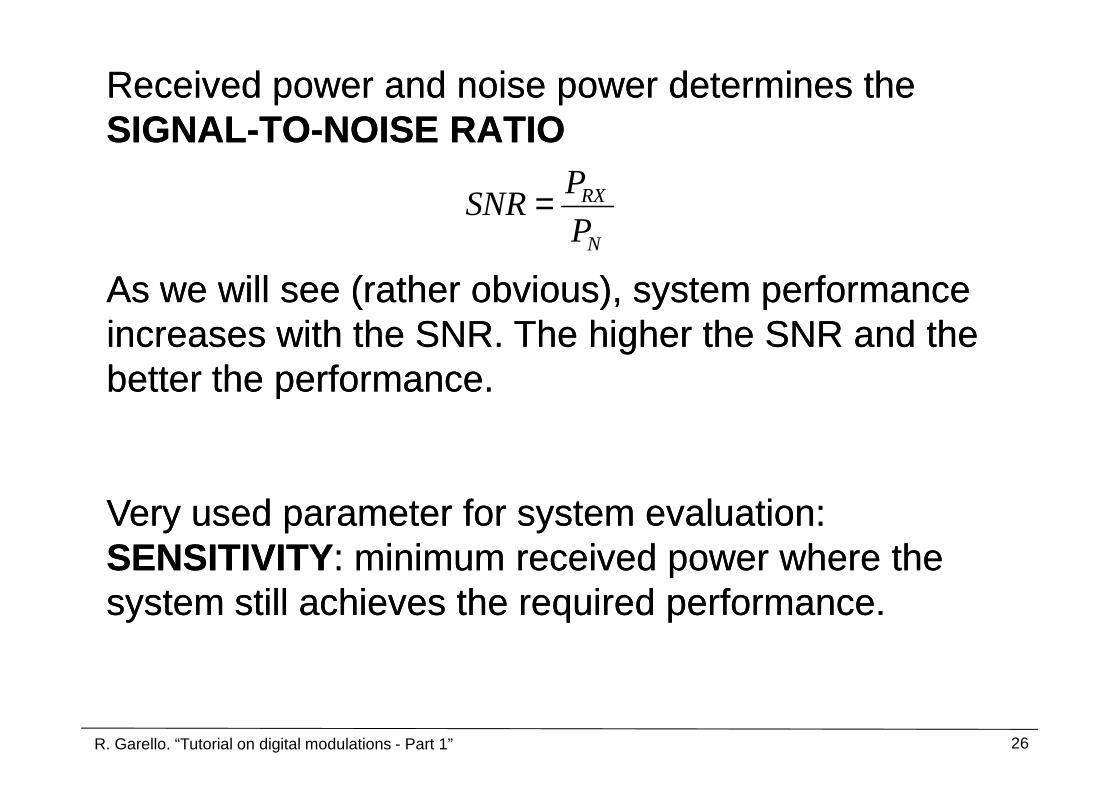
Received power and noise power determines theReceived power and noise power determines theSIGNALSIGNAL--TOTO--NOISE RATIONOISE RATIO

RX

N

PSNR

P=

As we will see (rather obvious), system performance As we will see (rather obvious), system performance increases with the SNR. The higher the increases with the SNR. The higher the SNR and SNR and the the better the performance.better the performance.


better the performance.better the performance.

Very used parameter for system evaluation:Very used parameter for system evaluation:SENSITIVITYSENSITIVITY: minimum received power where the : minimum received power where the system still achieves the required performance.system still achieves the required performance.

When transmitted over the channel, the waveform is changed. Main reasons:When transmitted over the channel, the waveform is changed. Main reasons:-- Channel frequency responseChannel frequency response-- NoiseNoise

As a consequence we may haveAs a consequence we may have

4 4 –– Error rateError rate

Tu ( )s t ( )r t Ru

R Tu u≠

( ) ( )r t s t≠


source TX RXCHANNEL

Tu ( )s t ( )r t Ru

( )[ ] [ ]R TBER P u i u i≡ ≠

Is the probability than an information bits is received wrongIs the probability than an information bits is received wrong

4 4 –– Error rateError rate

1E-5

1E-4

1E-3

0.01

0.1

1

BER

We will describe the error rate performance by curves like this one, where the We will describe the error rate performance by curves like this one, where the Bit Error rate is represented as a function of the received power:Bit Error rate is represented as a function of the received power:


-2 0 2 4 6 8 10 12 14 161E-14

1E-13

1E-12

1E-11

1E-10

1E-9

1E-8

1E-7

1E-6

1E-5

BE

R

Eb/N0 [dB] (proportional to P(proportional to PRXRX))

Modern systems require very low BER values (ex: MPEG Modern systems require very low BER values (ex: MPEG ��BERBER≅≅1010--1010))

5 5 –– ComplexityComplexity

Engineering complexity of practical implementation.(Consumed power/space in some frameworks)


source TX RXCHANNEL

Tu ( )s t ( )r t Ru

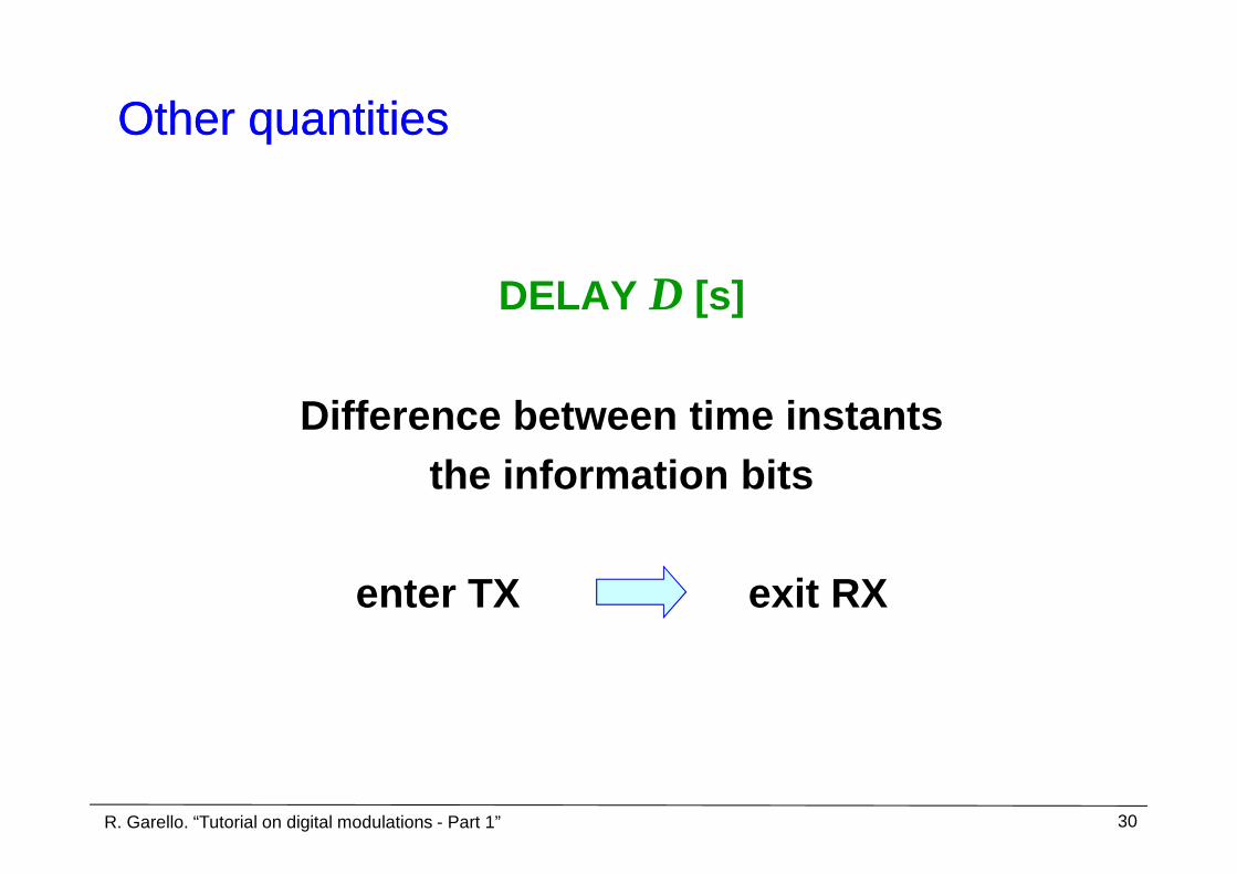
DELAY D [s]

Difference between time instants

Other quantitiesOther quantities


Difference between time instants the information bits

enter TX exit RX

AVAILABILITY [s]

Number of seconds where the system achieves the required performance

Other quantitiesOther quantities


the required performance

Given an AVAILABLE BANDWIDTH Ba=20 MHz, centered around f0=18 GHzDesign a digital transmission system which

• transmits a BIT-RATE R =34 Mbps

Practical examplePractical example


• transmits a BIT-RATE Rb=34 Mbps• guarantees at least BER = 10-7 for a received

POWER S=-40 dBm

• with maximum DELAY D=5 ms• with minimum COMPLEXITY (cost)

Documents

TUTORIAL ON DIGITAL MODULATIONS Part 1: … communication systems.pdf · TUTORIAL ON DIGITAL MODULATIONS Part 1: Introduction to digital communication systems. Fundamental quantities