Embed Size (px)
Citation preview
Tutorial on Machine Learning.
Part 1. Benchmarking of Different Machine Learning Regression Methods
Igor Baskin, Igor Tetko, Alexandre Varnek
1. Introduction
Nowadays there exist hundreds of different machine learning methods. Can one suggest
“the best” approach for QSAR/QSPR studies? The aim of this tutorial is to compare different
methods using the Experimenter mode of the Weka program. This tutorial is confined only to
regression tasks.
2. Machine Learning Methods
The following machine learning methods for performing regression are considered in the
tutorial:
1. Zero Regression (ZeroR) – pseudo-regression method that always builds models with
cross-validation coefficient Q2=0. In the framework of this method the value of a
property/activity is always predicted to be equal to its average value on the training set.
This method is usually used as a reference point for comparing with other regression
methods.
2. Multiple Linear Regression (MLR) with the M5 descriptor selection method and a fixed
small ridge parameter 0.00000001. In the M5 method, a MLR model is initially build on
all descriptors, and then descriptors with the smallest standardized regression coefficients
are step-wisely removed from the model until no improvement is observed in the estimate
of the average prediction error given by the Akaike information criterion.1
3. Partial Least Squares (PLS)2-5 with 5 latent variables.
4. Support Vector Regression (SVR)6 with the default value 1.0 of the trade-off parameter C,
the linear kernel and using the Shevade et al modification of the SMO algorithm.7
5. k Nearest Neighbors (kNN) with automatic selection of the optimal value of parameter k
through the internal cross-validation procedure and with the Euclidean distance computed
with all descriptors. Contributions of neighbors are weighted by the inverse of distance.
6. Back-Propagation Neural Network (BPNN) with one hidden layer with the default
number of sigmoid neurons trained with 500 epochs of the standard generalized delta-
rule algorithms with the learning rate 0.3 and momentum 0.2.
1
7. Regression Tree M5P (M5P) using the M5 algorithm.8
8. Regression by Discretization based on Random Forest (RD-RF). This is a regression
scheme that employs a classifier (random forest, in this case) on a copy of the data which
have the property/activity value discretized with equal width. The predicted value is the
expected value of the mean class value for each discretized interval (based on the
predicted probabilities for each interval). The random forest classification algorithm9 is
used here.
3. Datasets and Descriptors
The following structure-activity/property datasets are analyzed in the tutorial:
1. alkan-bp – the boiling points for 74 alkanes;10
2. alkan-mp – the melting points for 74 alkanes;10
3. selwood – the Selwood dataset of 33 antifilarial antimycin analogs;11
4. shapiro – the Shapiro dataset of 124 phenolic inhibitors of oral bacteria.12, 13
Evidently, alkan-bp and alkan-mp are structure-property datasets, while selwood and
shapiro are structure-activity ones. It is rather easy to build QSAR/QSPR models for alkan-bp
and alkan-mp, while alkan-mp and selwood pose a serious challenge for QSAR/QSPR modeling.
The Kier-Hall connectivity topological indexes (0χ, 1χ, 2χ, 3χp, 3χc, 4χp, 4χpc, 5χp, 5χc, 6χp)14, 15 are used as descriptors for the alkan-bp and alkan-mp datasets. Compounds from the
Selwood dataset11 are characterized by means of 52 physico-chemical descriptors.16 The Shapiro
dataset12 is characterized using 14 TLSER (Theoretical Linear Solvation Energy Relationships)
descriptors.17
4. Files
The following files are supplied for the tutorial
• alkan-bp-connect.arff – descriptor and property values for the alkan-bp dataset;
• alkan-mp-connect.arff – descriptor and property values for the alkan-mp dataset;
• selwood.arff –descriptors and activities for the selwood database;
• shapiro.arff –descriptors and activities for the shapiro database;
• compare1.exp – experiment configuration file
• compare1-results.arff – file with results
2

5. Step-by-Step Instructions
In this tutorial, the Experimenter mode of the Weka program is used. This mode allows
one to apply systematically machine learning to different datasets, to repeat this several times,
and compare relative performances of different approaches. This study includes the following
steps: (1) initialization of the Experimenter mode, (2) specification of the list of datasets to be
processed, (3) specification of the list of machine learning methods to be applied to selected
datasets, (4) running machine learning methods, (5) analysis of obtained results.
5.1. Initialization of the Experimenter mode
• Start Weka.
• Select the item Experimenter in the menu Applications.
• Press button New in order to create a new experiment configuration file.
• Enter the name of the result file: compare1-results.arff.
• Enter the number of cross-validation folds: 5.
• Choose the appropriate mode by selecting the radio-button Regression.
• Press button Save… and then specify the name of the experiment configuration file
compare1.exp
At this point, the main window of the program looks like that:
3
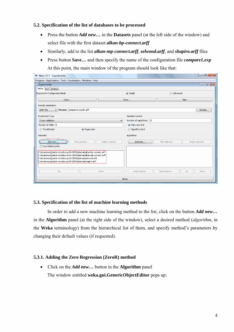
5.2. Specification of the list of databases to be processed
• Press the button Add new… in the Datasets panel (at the left side of the window) and
select file with the first dataset alkan-bp-connect.arff
• Similarly, add to the list alkan-mp-connect.arff, selwood.arff, and shapiro.arff files
• Press button Save… and then specify the name of the configuration file compare1.exp
At this point, the main window of the program should look like that:
5.3. Specification of the list of machine learning methods
In order to add a new machine learning method to the list, click on the button Add new…
in the Algorithm panel (at the right side of the window), select a desired method (algorithm, in
the Weka terminology) from the hierarchical list of them, and specify method’s parameters by
changing their default values (if requested).
5.3.1. Adding the Zero Regression (ZeroR) method
• Click on the Add new… button in the Algorithm panel
The window entitled weka.gui.GenericObjectEditor pops up:
4
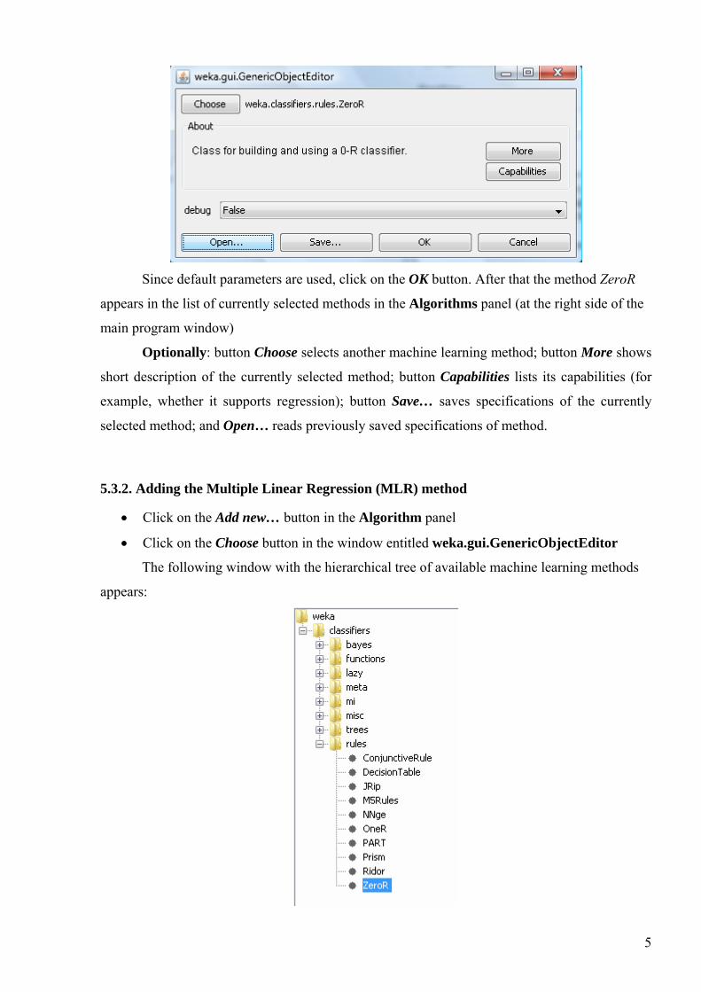
Since default parameters are used, click on the OK button. After that the method ZeroR
appears in the list of currently selected methods in the Algorithms panel (at the right side of the
main program window)
Optionally: button Choose selects another machine learning method; button More shows
short description of the currently selected method; button Capabilities lists its capabilities (for
example, whether it supports regression); button Save… saves specifications of the currently
selected method; and Open… reads previously saved specifications of method.
5.3.2. Adding the Multiple Linear Regression (MLR) method
• Click on the Add new… button in the Algorithm panel
• Click on the Choose button in the window entitled weka.gui.GenericObjectEditor
The following window with the hierarchical tree of available machine learning methods
appears:
5
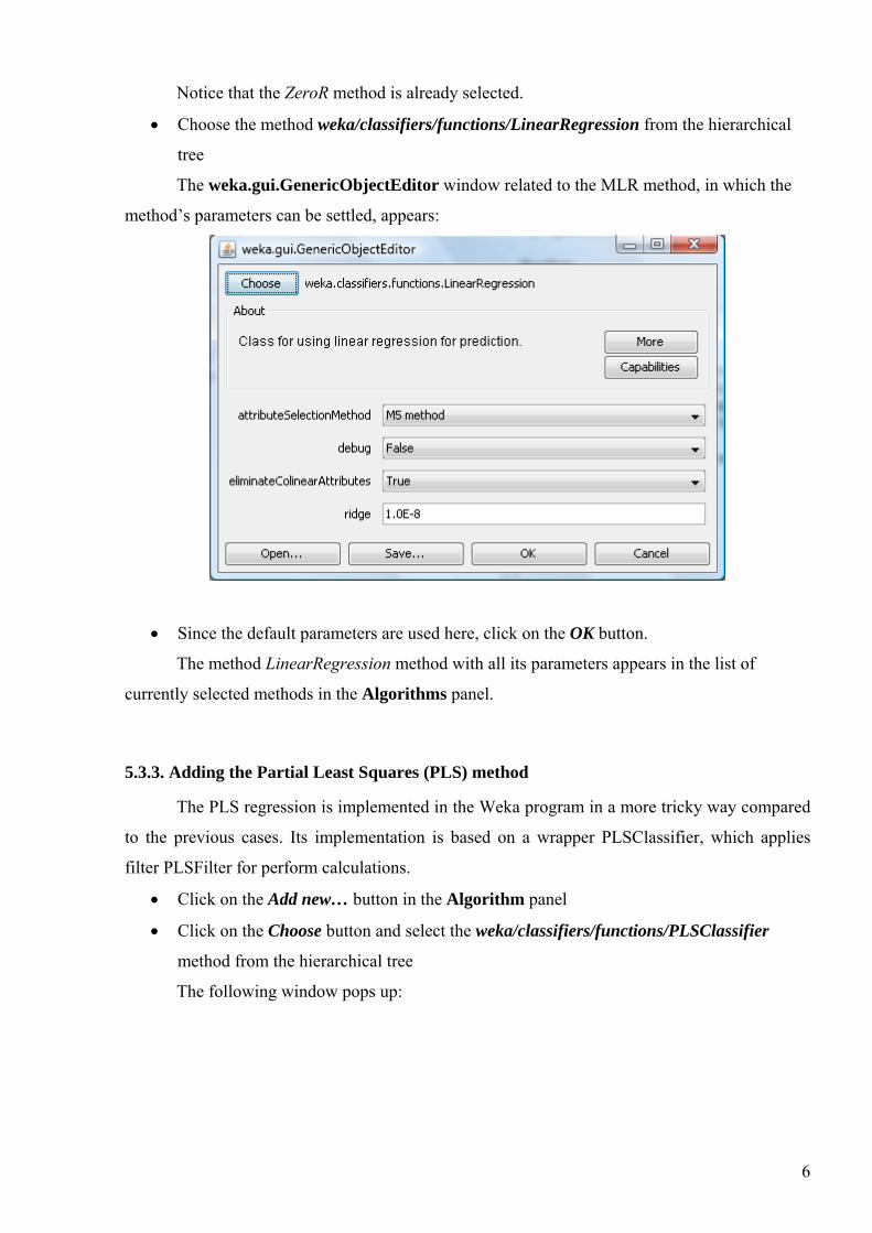
Notice that the ZeroR method is already selected.
• Choose the method weka/classifiers/functions/LinearRegression from the hierarchical
tree
The weka.gui.GenericObjectEditor window related to the MLR method, in which the
method’s parameters can be settled, appears:
• Since the default parameters are used here, click on the OK button.
The method LinearRegression method with all its parameters appears in the list of
currently selected methods in the Algorithms panel.
5.3.3. Adding the Partial Least Squares (PLS) method
The PLS regression is implemented in the Weka program in a more tricky way compared
to the previous cases. Its implementation is based on a wrapper PLSClassifier, which applies
filter PLSFilter for perform calculations.
• Click on the Add new… button in the Algorithm panel
• Click on the Choose button and select the weka/classifiers/functions/PLSClassifier
method from the hierarchical tree
The following window pops up:
6
The default settings for PLSFilters imply 20 components (latent variables) (see the key –
C 20). In this tutorial, we will set the number of components to be 5.
• Click on PLSFilter. A window containing different parameters of the PLS method
appears.
• Set the number of components to 5
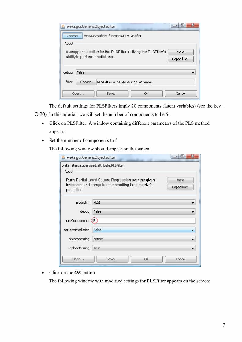
The following window should appear on the screen:
• Click on the OK button
The following window with modified settings for PLSFilter appears on the screen:
7
• Click on the OK button
After that the PLSClassifier method with all its parameters appears in the list of currently
selected methods in the Algorithms panel
Optionally, Weka allows user to find the “optimal” number of latent variables by means
of a special meta-procedure.
5.3.4. Adding the Support Vector Regression (SVR) method
• Click on the Add new… button in the Algorithm panel
• Click on the Choose button in the window entitled weka.gui.GenericObjectEditorand
choose the weka/classifiers/functions/SVMreg method from the hierarchical tree
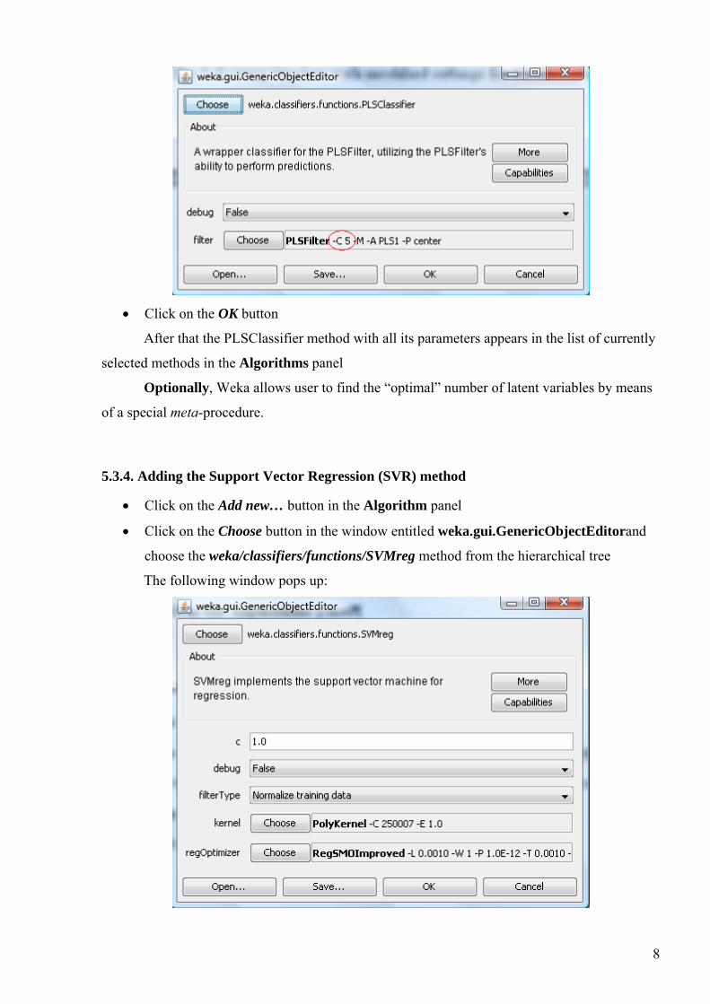
The following window pops up:
8
In this tutorial, the default values for all parameters are used: of the error-complexity
tradeoff parameter C is 1.0, the type of kernel is polynomial with degree 1 (i.e. the linear kernel),
the value of the ε parameter for the ε-insensitive loss function (key -L) is 0.0010.
• Click on the OK button
After that the SVMreg method with all its parameters appears in the list of currently
selected methods in the Algorithms panel
Optionally, one can either apply a special wrapper procedure for finding the optional
values of parameter C, ε and a kernel-specific parameter (degree for the polynomial kernel and γ
for the Gaussian [RBF – Radial Basis Function] kernel), or one can define the SVR algorithm
with a certain set of parameter values as a separate method, and run all of them sequentially.
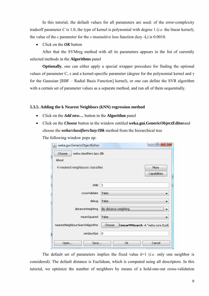
5.3.5. Adding the k Nearest Neighbors (kNN) regression method
• Click on the Add new… button in the Algorithm panel
• Click on the Choose button in the window entitled weka.gui.GenericObjectEditorand
choose the weka/classifiers/lazy/IBk method from the hierarchical tree
The following window pops up:
The default set of parameters implies the fixed value k=1 (i.e. only one neighbor is
considered). The default distance is Euclidean, which is computed using all descriptors. In this
tutorial, we optimize the number of neighbors by means of a hold-one-out cross-validation
9
procedure varying k from 1 to 10. The weighted version of the kNN regression with weights
inversely proportional to distances is suggested.
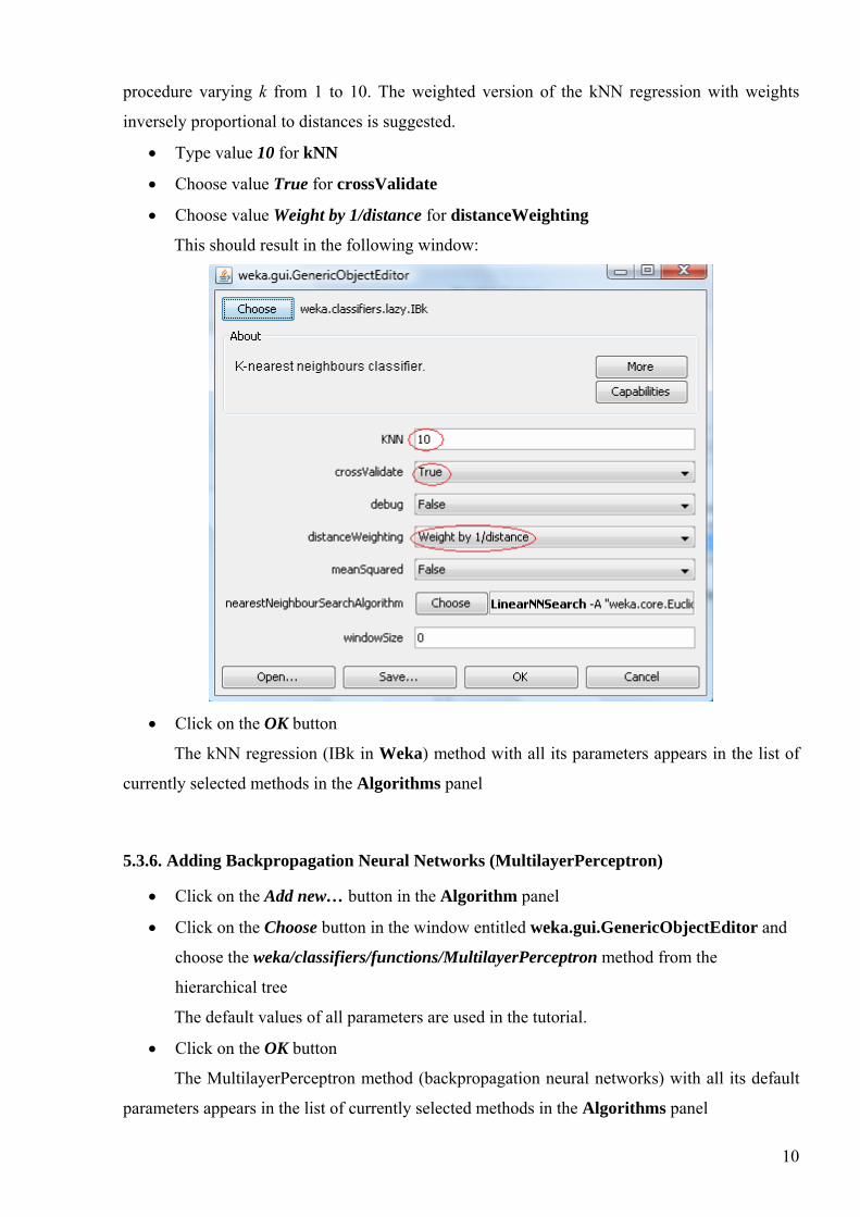
• Type value 10 for kNN
• Choose value True for crossValidate
• Choose value Weight by 1/distance for distanceWeighting
This should result in the following window:
• Click on the OK button
The kNN regression (IBk in Weka) method with all its parameters appears in the list of
currently selected methods in the Algorithms panel
5.3.6. Adding Backpropagation Neural Networks (MultilayerPerceptron)
• Click on the Add new… button in the Algorithm panel
• Click on the Choose button in the window entitled weka.gui.GenericObjectEditor and
choose the weka/classifiers/functions/MultilayerPerceptron method from the
hierarchical tree
The default values of all parameters are used in the tutorial.
• Click on the OK button
The MultilayerPerceptron method (backpropagation neural networks) with all its default
parameters appears in the list of currently selected methods in the Algorithms panel
10
5.3.7. Adding the Regression Trees method (M5P)
• Click on the Add new… button in the Algorithm panel
• Click on the Choose button in the window entitled weka.gui.GenericObjectEditor and
choose the weka/classifiers/trees/M5P method from the hierarchical tree
At this stage, a window containing numerous options for building and running regression
trees pops up. The default values are used in this tutorial.
• Click on the OK button
The M5P regression trees method with all its default parameters appears in the list of
currently selected methods in the Algorithms panel
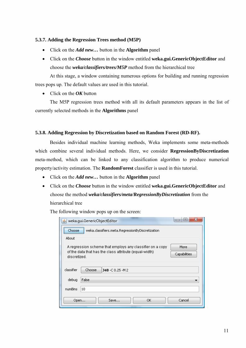
5.3.8. Adding Regression by Discretization based on Random Forest (RD-RF).
Besides individual machine learning methods, Weka implements some meta-methods
which combine several individual methods. Here, we consider RegressionByDiscretization
meta-method, which can be linked to any classification algorithm to produce numerical
property/activity estimation. The RandomForest classifier is used in this tutorial.
• Click on the Add new… button in the Algorithm panel
• Click on the Choose button in the window entitled weka.gui.GenericObjectEditor and
choose the method weka/classifiers/meta/RegressionByDiscretization from the
hierarchical tree
The following window pops up on the screen:
11
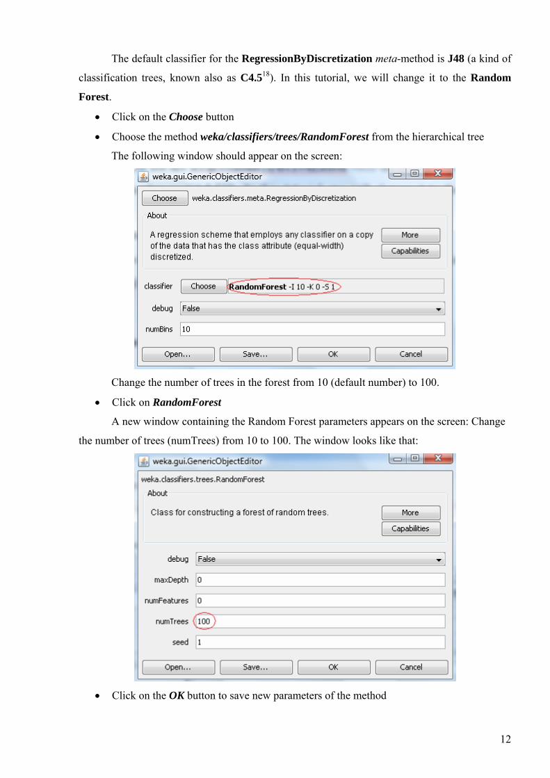
The default classifier for the RegressionByDiscretization meta-method is J48 (a kind of
classification trees, known also as C4.518). In this tutorial, we will change it to the Random
Forest.
• Click on the Choose button
• Choose the method weka/classifiers/trees/RandomForest from the hierarchical tree
The following window should appear on the screen:
Change the number of trees in the forest from 10 (default number) to 100.
• Click on RandomForest
A new window containing the Random Forest parameters appears on the screen: Change
the number of trees (numTrees) from 10 to 100. The window looks like that:
• Click on the OK button to save new parameters of the method
12
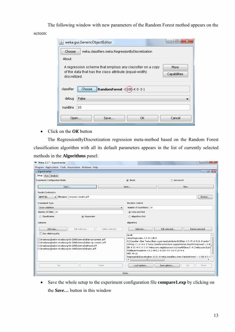
The following window with new parameters of the Random Forest method appears on the
screen:
• Click on the OK button
The RegressionByDiscretization regression meta-method based on the Random Forest
classification algorithm with all its default parameters appears in the list of currently selected
methods in the Algorithms panel:
• Save the whole setup to the experiment configuration file compare1.exp by clicking on
the Save… button in this window
13

5.4. Running machine learning methods
Since the setup for the experimenter mode has been prepared, one can apply selected
machine learning methods to the set of datasets.
• Switch to the Run mode by clicking on the Run label
• Click on the Start button
Execution of the experiment starts:
The current status of the process is indicated at the bottom side of the window. The
history is written to the central log window. The selected machine learning methods are applied
to each of the selected datasets 10 times, each time a dataset is randomized. Successful
termination of the job is indicated on the log window:
5.5. Analysis of obtained results
• Switch to the Analyse panel
• Load the result file compare1-result.arff by clicking on the File… button and selecting
the appropriate file
The current window is the following:
14

The Configure test panel (on the left) contains the options for running comparison test,
while the test output (on the right) contains the list of machine learning methods just executed
against the datasets. The Configure test panel has different options to assess relative
performance of machine learning methods. The most important ones are the following:
1. Testing with - statistical method used to compare performances of machine learning
methods. Default is Paired T-tester (corrected) based on Student’s t-criterion.
2. Comparison field - performance measure. The default value is
Root_relative_squared_error (which is related to Q2). Other options include
Relative_absolute_error and Correlation_coefficient (between predicted and
experimental values). All performance measures are computed using the cross-validation
procedure!
3. Significance - Significance value used for t-test
5.5.1. Root_relative_squared_error performance measure
• Run test by clicking on the Perform test button
• Read and analyze the content of the Test output panel
The obtained results can be represented by means of the following table (rank is in the
parenthesis, values not passing the t-test are shown in italic):
15
alkan-bp alkan-mp selwood shapiro
ZeroR 100.00 (8) 100.00 (6) 100.00 (5) 100.00 (8)
MLR 20.38 (6) 112.64 (8) 221.18 (8) 48.86 (5)
PLS 13.40 (4) 105.06 (7) 91.17 (3) 43.00 (1)
SVR 10.16 (2) 95.81 (3.5) 99.01 (4) 47.06 (3)
kNN 21.45 (7) 95.81 (3.5) 88.45 (2) 50.95 (6)
BPNN 8.79 (1) 90.76 (2) 117.95 (6) 64.26 (7)
M5P 10.29 (3) 102.24 (5) 127.48 (7) 47.69 (4)
RD-RF 19.70 (5) 89.67 (1) 77.39 (1) 45.59 (2)
The obtained results can slightly deviate for those depicted in the Table because of the
stochastic nature of randomization.
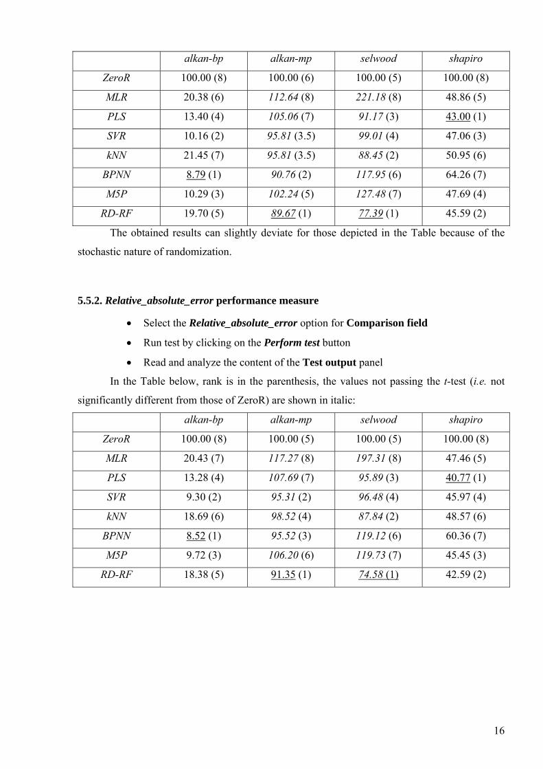
5.5.2. Relative_absolute_error performance measure
• Select the Relative_absolute_error option for Comparison field
• Run test by clicking on the Perform test button
• Read and analyze the content of the Test output panel
In the Table below, rank is in the parenthesis, the values not passing the t-test (i.e. not
significantly different from those of ZeroR) are shown in italic:
alkan-bp alkan-mp selwood shapiro
ZeroR 100.00 (8) 100.00 (5) 100.00 (5) 100.00 (8)
MLR 20.43 (7) 117.27 (8) 197.31 (8) 47.46 (5)
PLS 13.28 (4) 107.69 (7) 95.89 (3) 40.77 (1)
SVR 9.30 (2) 95.31 (2) 96.48 (4) 45.97 (4)
kNN 18.69 (6) 98.52 (4) 87.84 (2) 48.57 (6)
BPNN 8.52 (1) 95.52 (3) 119.12 (6) 60.36 (7)
M5P 9.72 (3) 106.20 (6) 119.73 (7) 45.45 (3)
RD-RF 18.38 (5) 91.35 (1) 74.58 (1) 42.59 (2)
16
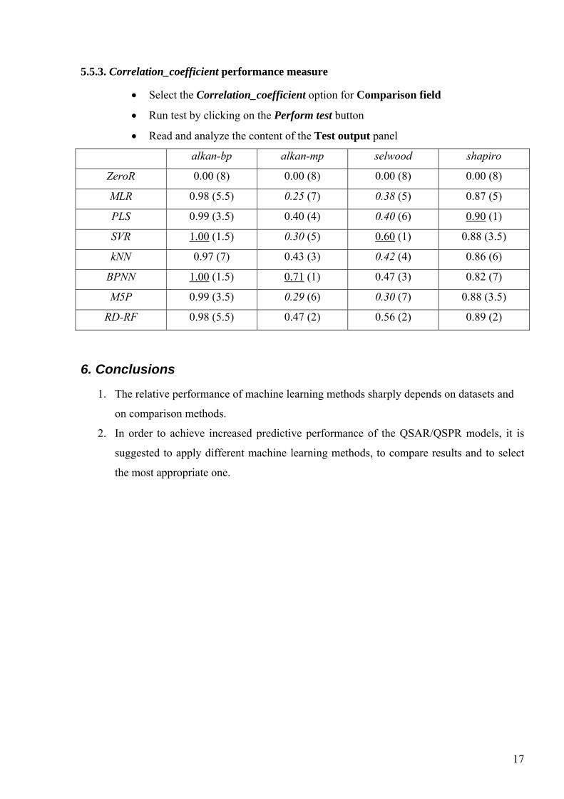
5.5.3. Correlation_coefficient performance measure
• Select the Correlation_coefficient option for Comparison field
• Run test by clicking on the Perform test button
• Read and analyze the content of the Test output panel
alkan-bp alkan-mp selwood shapiro
ZeroR 0.00 (8) 0.00 (8) 0.00 (8) 0.00 (8)
MLR 0.98 (5.5) 0.25 (7) 0.38 (5) 0.87 (5)
PLS 0.99 (3.5) 0.40 (4) 0.40 (6) 0.90 (1)
SVR 1.00 (1.5) 0.30 (5) 0.60 (1) 0.88 (3.5)
kNN 0.97 (7) 0.43 (3) 0.42 (4) 0.86 (6)
BPNN 1.00 (1.5) 0.71 (1) 0.47 (3) 0.82 (7)
M5P 0.99 (3.5) 0.29 (6) 0.30 (7) 0.88 (3.5)
RD-RF 0.98 (5.5) 0.47 (2) 0.56 (2) 0.89 (2)
6. Conclusions
1. The relative performance of machine learning methods sharply depends on datasets and
on comparison methods.
2. In order to achieve increased predictive performance of the QSAR/QSPR models, it is
suggested to apply different machine learning methods, to compare results and to select
the most appropriate one.
17
7. References
1. Akaike, H., A new look at the statistical model identification. IEEE Transactions on Automatic Control 1974, 19, (6), 716–723. 2. Wold, H., Estimation of principal components and related models by iterative least squares. In Multivariate Analysis, Krishnaiaah, P. R., Ed. Academic Press: New York, 1966; pp 391-420. 3. Geladi, P.; Kowlaski, B., Partial least square regression: A tutorial. Analytica Chemica Acta 1986, 35, 1-17. 4. Höskuldsson, A., PLS regression methods. J. Chemometrics 1988, 2, (3), 211-228. 5. Helland, I. S., PLS regression and statistical models. Scandivian Journal of Statistics 1990, 17, 97-114. 6. Smola, A. J.; Schölkopf, B., A tutorial on support vector regression. Statistics and Computing 2004, 14, (3), 199-222. 7. Shevade, S. K.; Keerthi, S. S.; Bhattacharyya, C.; Murthy, K. R. K., Improvements to the SMO algorithm for SVM regression. IEEE Transactions on Neural Networks 2000, 11, (5), 1188-1193. 8. Quinlan, J. R., Learning with continuous classes. Proceedings AI'92 1992, 343-348. 9. Breiman, L., Random forests. Machine Learning 2001, 45, (1), 5-32. 10. Needham, D. E.; Wei, I. C.; Seybold, P. G., Molecular modeling of the physical properties of alkanes. J. Am. Chem. Soc. 1988, 110, (13), 4186-4194. 11. Selwood, D. L.; Livingstone, D. J.; Comley, J. C. W.; O'Dowd, A. B.; Hudson, A. T.; Jackson, P.; Jandu, K. S.; Rose, V. S.; Stables, J. N., Structure-activity relationships of antifilarial antimycin analogs: a multivariate pattern recognition study. J. Med. Chem. 1990, 33, (1), 136-142. 12. Shapiro, S.; Guggenheim, B., Inhibition of oral bacteria by phenolic compounds. Part 1. QSAR analysis using molecular connectivity. Quantitative Structure-Activity Relationships 1998, 17, (4), 327-337. 13. Shapiro, S.; Guggenheim, B., Inhibition of oral bacteria by phenolic compounds. Part 2. Correlations with molecular descriptors. Quantitative Structure-Activity Relationships 1998, 17, (4), 338-347. 14. Kier, L. B.; Hall, L. H., Molecular Connectivity in Chemistry and Drug Research. Academic Press: New York (NY), 1976; p 257. 15. Kier, L. B.; Hall, L. H., Molecular connectivity in structure-activity analysis. Research Studies Press: Letchworth, 1986. 16. Kubinyi, H., Evolutionary variable selection in regression and PLS analyses. Journal of Chemometrics 1996, 10, (2), 119-133. 17. Famini, G. R.; Wilson, L. Y., Using theoretical descriptors in linear solvation energy relationships. In Theoretical and Computational Chemistry, Politzer, P.; Murray, J. S., Eds. Elsevier: 1994; Vol. 1, pp 213-241. 18. Quinlan, R., C4.5: Programs for Machine Learning. Morgan Kaufmann Publishers: San Mateo, CA, 1993.
18