Embed Size (px)
Citation preview

Tutorial Graph Based Image Segmentation
Jianbo Shi, David Martin, Charless Fowlkes, Eitan Sharon
Topics
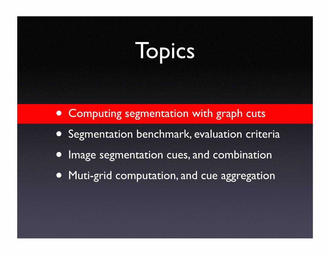
• Computing segmentation with graph cuts
• Segmentation benchmark, evaluation criteria
• Image segmentation cues, and combination
• Muti-grid computation, and cue aggregation
Wij
Wiji
j
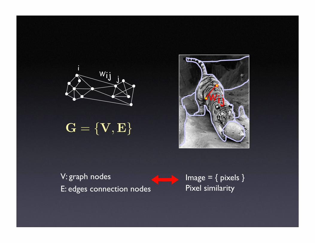
G = {V,E}
V: graph nodes
E: edges connection nodes Image = { pixels }Pixel similarity
Topics
• Computing segmentation with graph cuts
• Segmentation benchmark, evaluation criteria
• Image segmentation cues, and combination
• Muti-grid computation, and cue aggregation
Topics
• Computing segmentation with graph cuts
• Segmentation benchmark, evaluation criteria
• Image segmentation cues, and combination
• Muti-grid computation, and cue aggregation
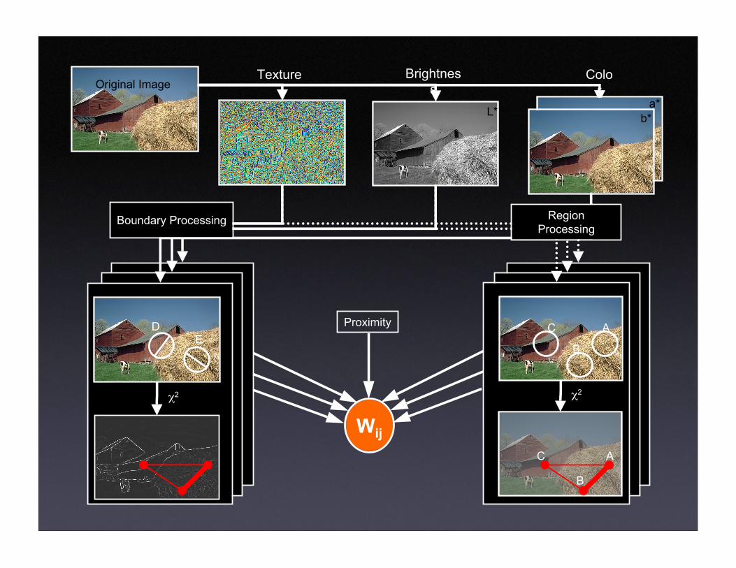
Color
a*b*
Brightness
L*
TextureOriginal Image
Wij
Proximity
ED
χ2
Boundary Processing
Textons
A
B
C
A
B
C
χ2
RegionProcessing
Topics
• Computing segmentation with graph cuts
• Segmentation benchmark, evaluation criteria
• Image segmentation cues, and combination
• Muti-grid computation, and cue aggregation

Part I: Graph and Images
Jianbo Shi
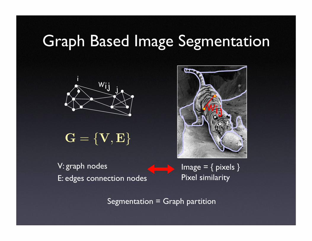
Graph Based Image Segmentation
Wij
Wiji
j
G = {V,E}
V: graph nodes
E: edges connection nodes Image = { pixels }Pixel similarity
Segmentation = Graph partition
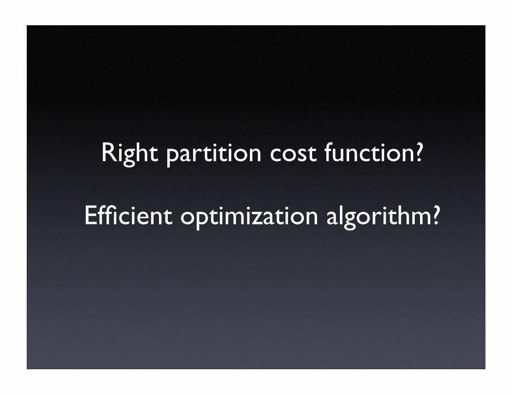
Right partition cost function?
Efficient optimization algorithm?

Graph Terminology
adjacency matrix, degree, volume,
graph cuts
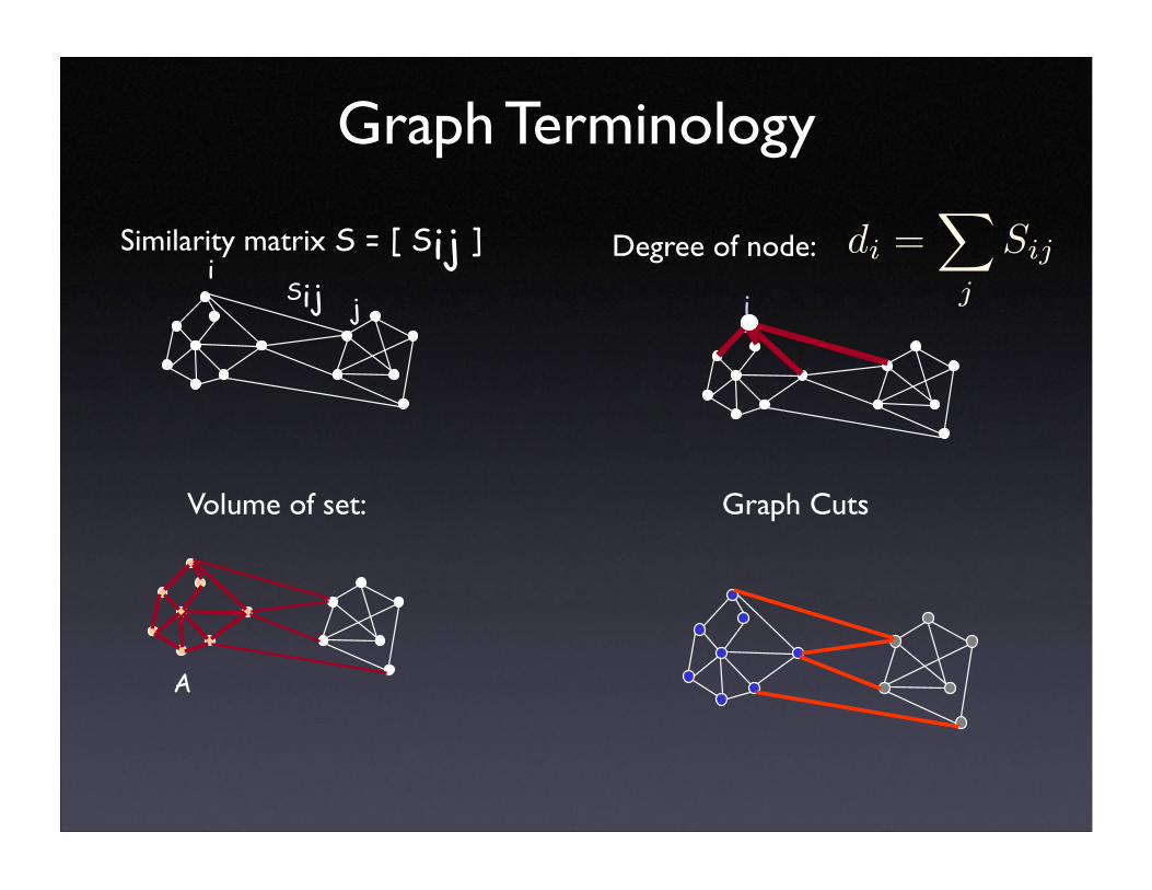
Graph Terminology
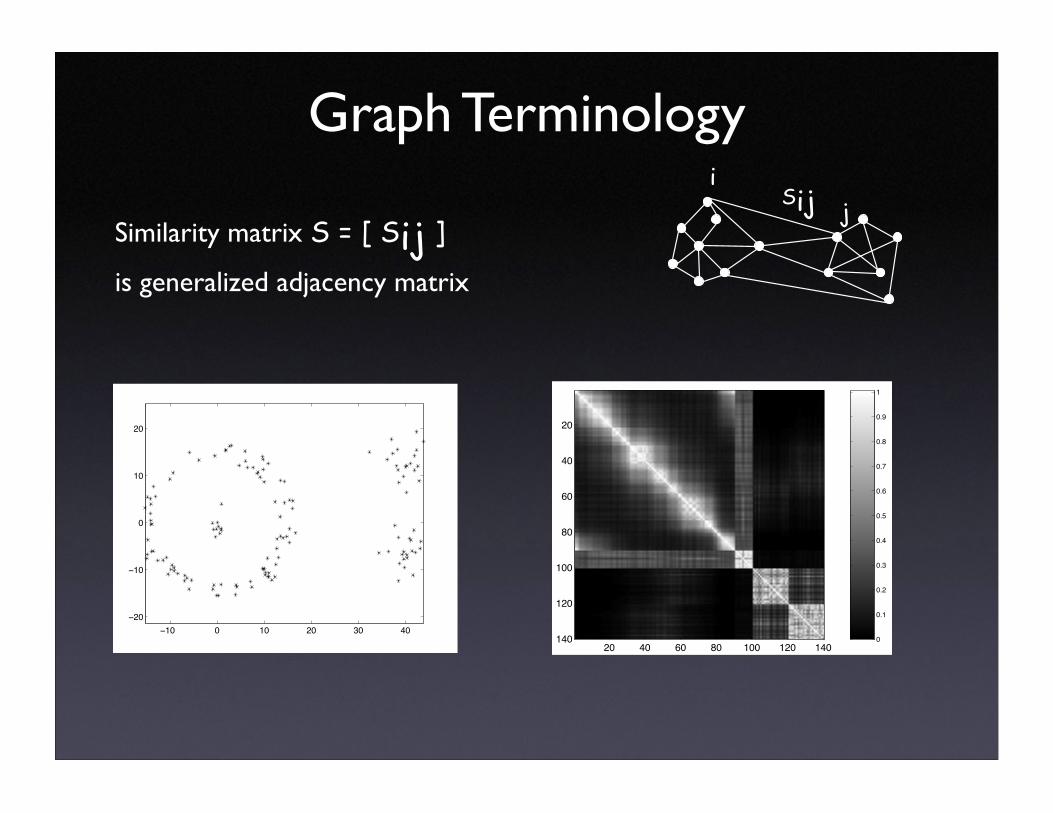
Similarity matrix S = [ Sij ]
is generalized adjacency matrix
Siji
j
!10 0 10 20 30 40
!20
!10
0
10
20
20 40 60 80 100 120 140
20
40
60
80
100
120
140 0
0.1
0.2
0.3
0.4
0.5
0.6
0.7
0.8
0.9
1
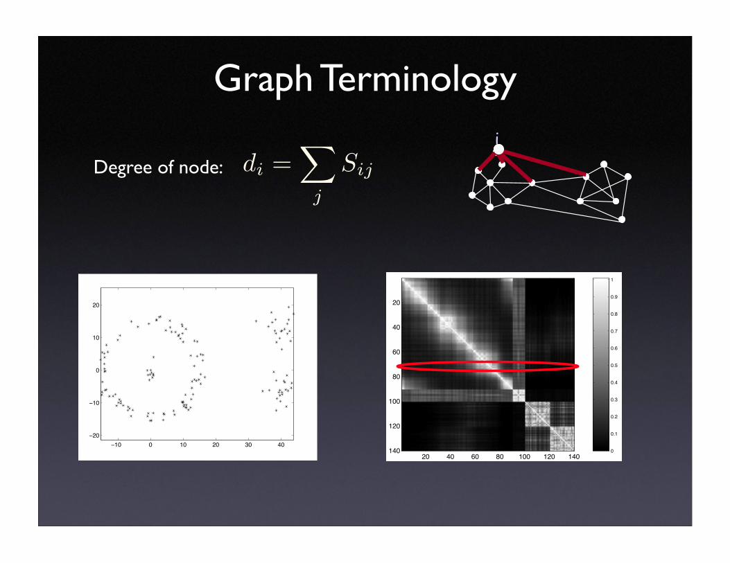
Graph Terminologyi
Degree of node: di =
∑
j
Sij
!10 0 10 20 30 40
!20
!10
0
10
20
20 40 60 80 100 120 140
20
40
60
80
100
120
140 0
0.1
0.2
0.3
0.4
0.5
0.6
0.7
0.8
0.9
1
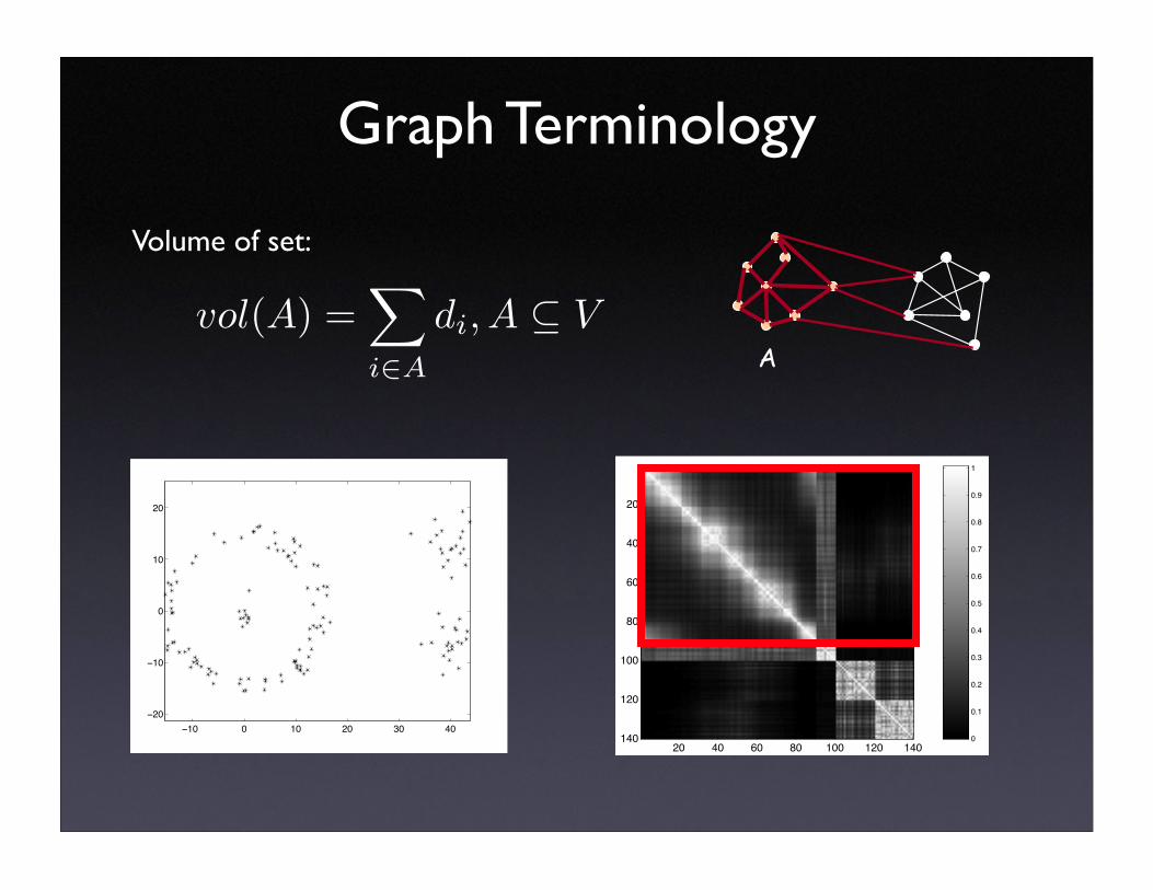
Graph Terminology
A
Volume of set:
vol(A) =∑
i∈A
di, A ⊆ V
!10 0 10 20 30 40
!20
!10
0
10
20
20 40 60 80 100 120 140
20
40
60
80
100
120
140 0
0.1
0.2
0.3
0.4
0.5
0.6
0.7
0.8
0.9
1
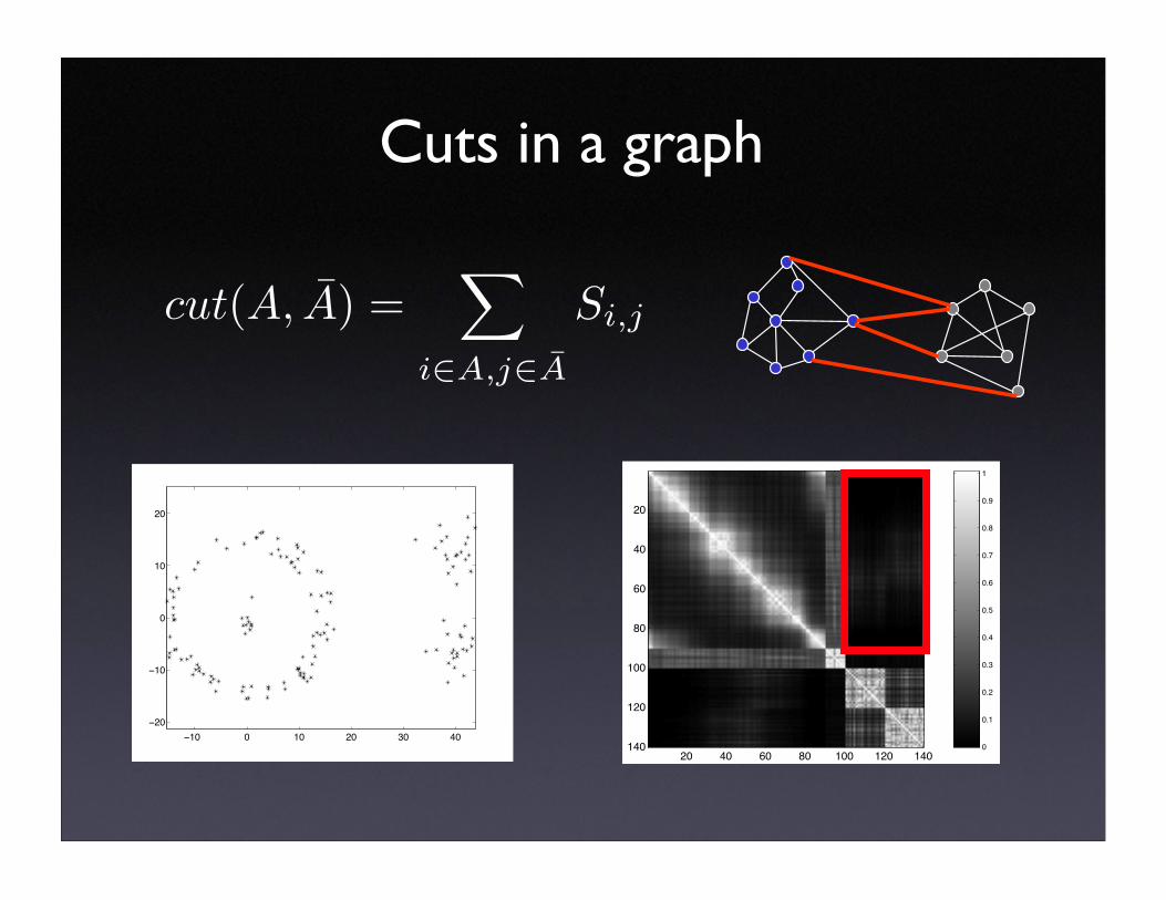
Cuts in a graph
cut(A, A) =∑
i∈A,j∈A
Si,j
!10 0 10 20 30 40
!20
!10
0
10
20
20 40 60 80 100 120 140
20
40
60
80
100
120
140 0
0.1
0.2
0.3
0.4
0.5
0.6
0.7
0.8
0.9
1
Graph Terminology
Similarity matrix S = [ Sij ]Sij
ij i
A
Volume of set:
Degree of node: di =
∑
j
Sij
Graph Cuts
Useful Graph Algorithms
• Minimal Spanning Tree
• Shortest path
• s-t Max. graph flow, Min. cut
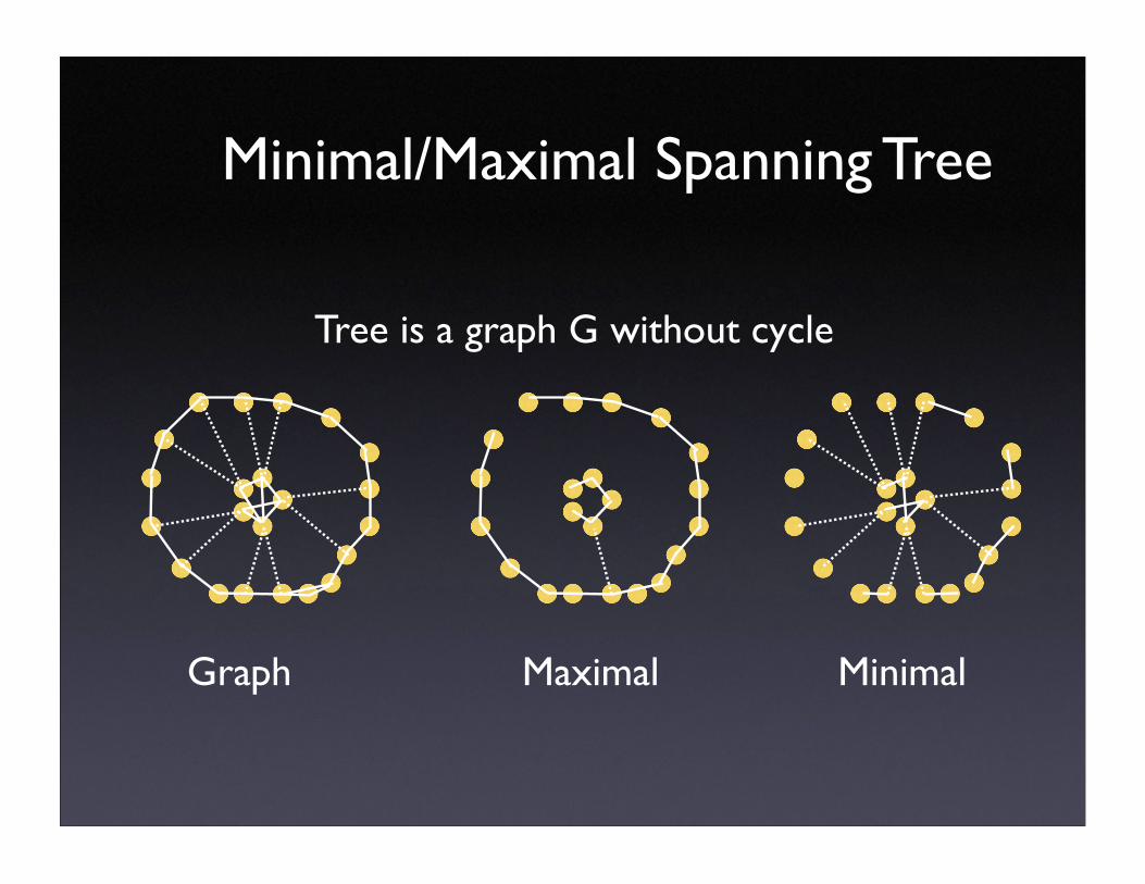
Minimal/Maximal Spanning Tree
Maximal Minimal
Tree is a graph G without cycle
Graph
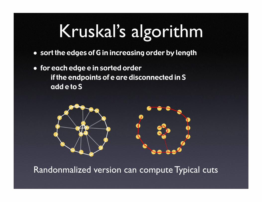
Kruskal’s algorithm• sort the edges of G in increasing order by length
• for each edge e in sorted order if the endpoints of e are disconnected in S add e to S
Randonmalized version can compute Typical cuts
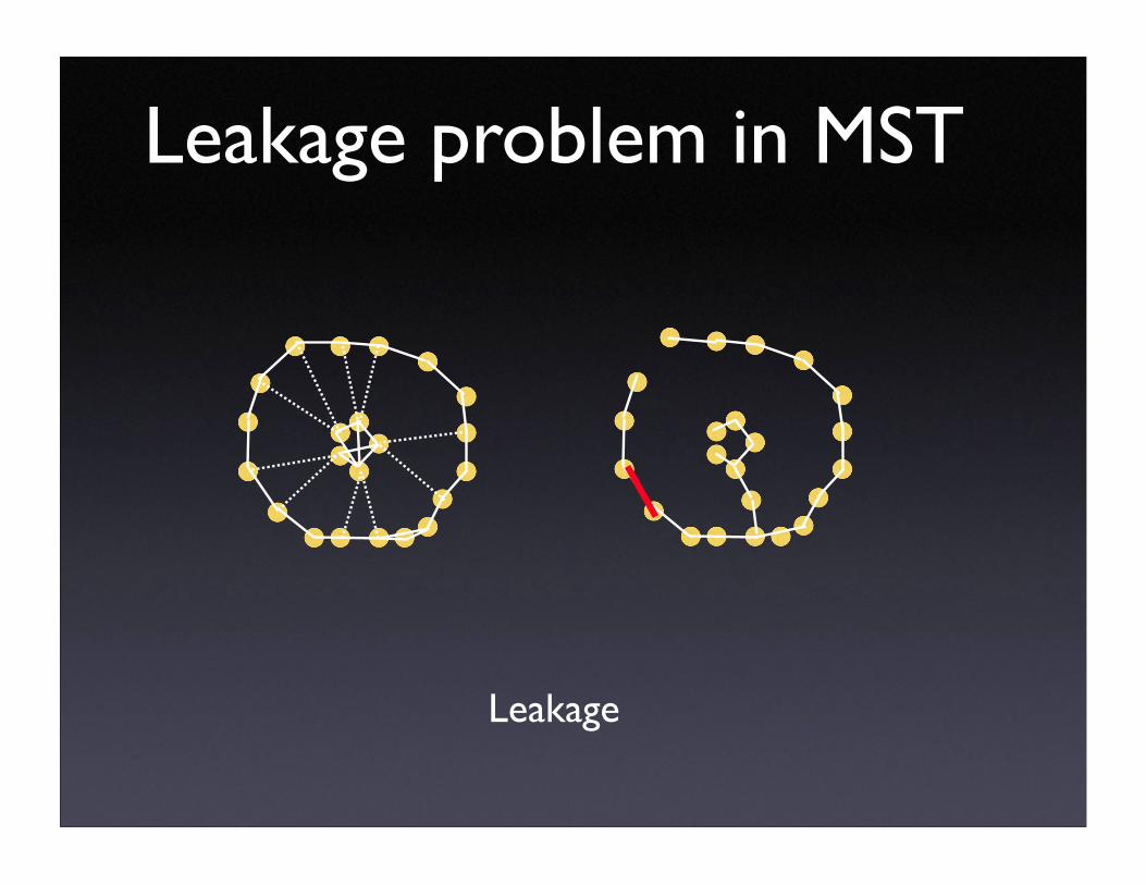
Leakage problem in MST
Leakage
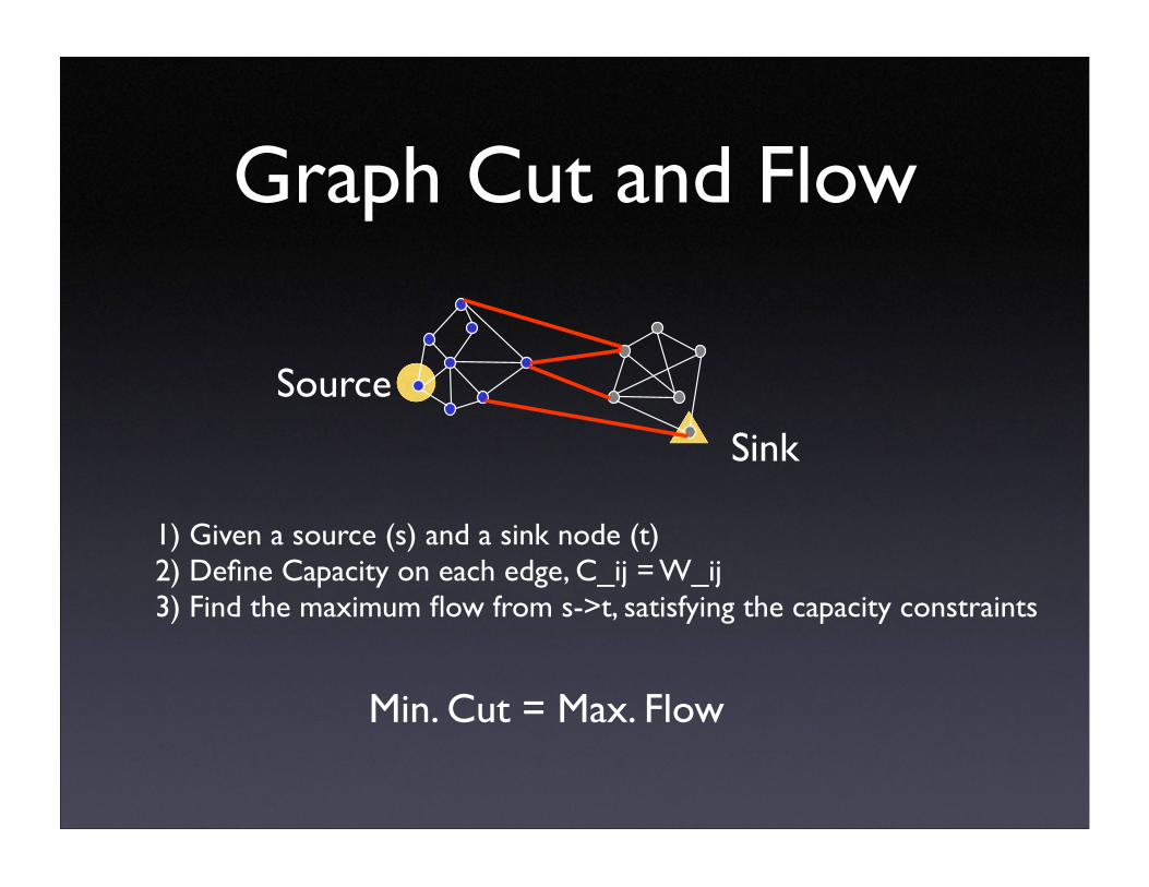
Graph Cut and Flow
Sink
Source
1) Given a source (s) and a sink node (t)2) Define Capacity on each edge, C_ij = W_ij3) Find the maximum flow from s->t, satisfying the capacity constraints
Min. Cut = Max. Flow
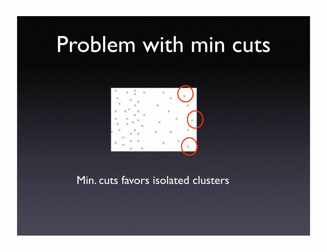
Problem with min cuts
Min. cuts favors isolated clusters
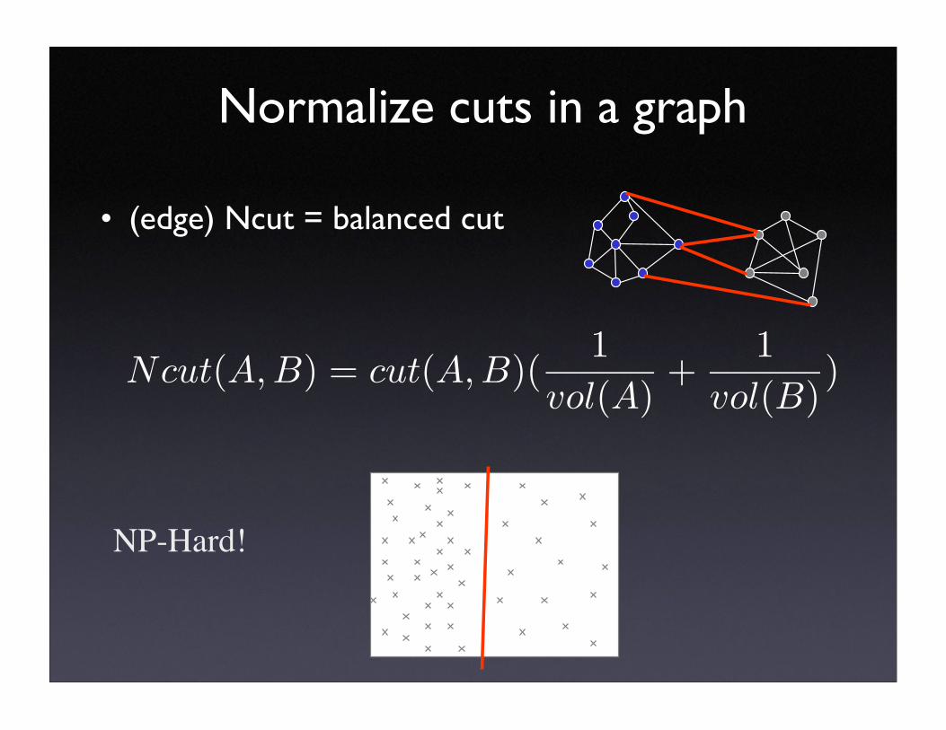
Normalize cuts in a graph
• (edge) Ncut = balanced cut
Ncut(A, B) = cut(A, B)(1
vol(A)+
1
vol(B))
NP-Hard!
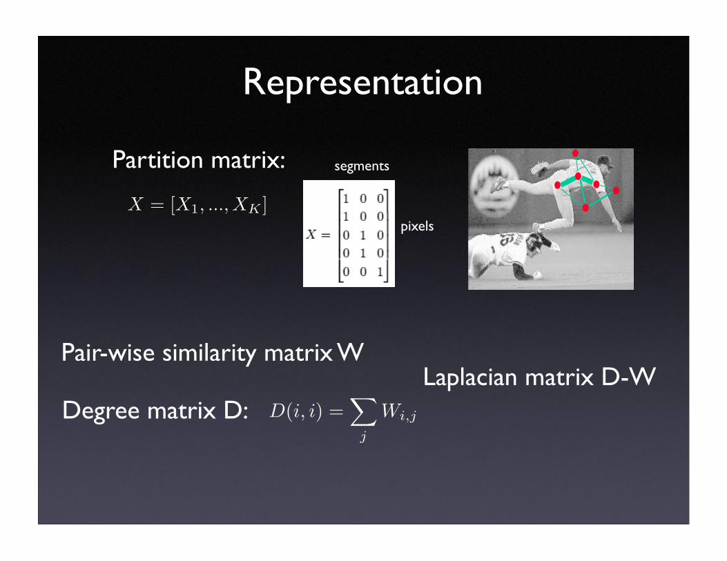
Representation
Partition matrix:
Laplacian matrix D-W
X = [X1, ..., XK ]
Pair-wise similarity matrix W
Degree matrix D: D(i, i) =∑
j
Wi,j
segments
pixels
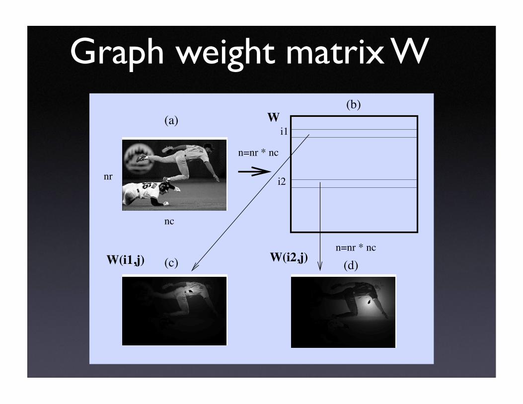
nr
W(b)
n=nr * nc
i2
i1
n=nr * nc
W(i1,j) W(i2,j)
nc
(c)
(a)
(d)
Graph weight matrix W
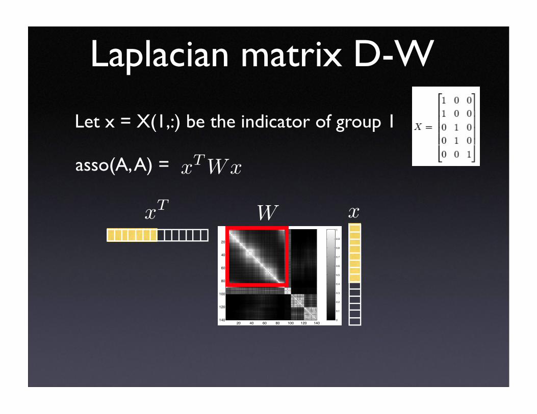
Laplacian matrix D-W
asso(A, A) =
Let x = X(1,:) be the indicator of group 1
xTWx
20 40 60 80 100 120 140
20
40
60
80
100
120
140 0
0.1
0.2
0.3
0.4
0.5
0.6
0.7
0.8
0.9
1
xT
xW
20 40 60 80 100 120 140
20
40
60
80
100
120
140 0
0.1
0.2
0.3
0.4
0.5
0.6
0.7
0.8
0.9
1
asso(A,A)x
TWx
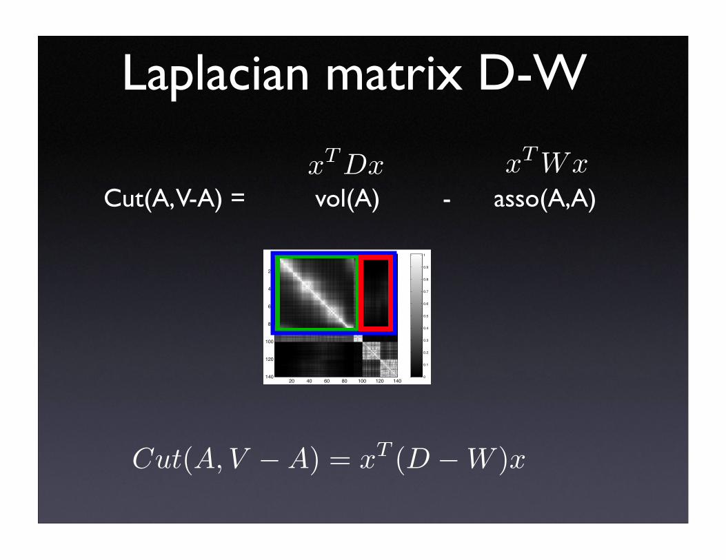
Laplacian matrix D-W
vol(A) x
TDx
Cut(A, V-A) = -
Cut(A, V − A) = xT (D − W )x
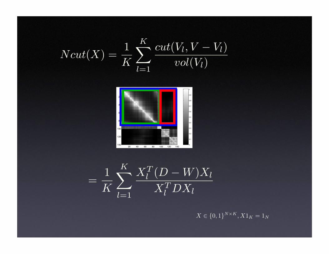
Ncut(X) =1
K
K∑
l=1
cut(Vl, V − Vl)
vol(Vl)
=1
K
K∑
l=1
XTl
(D − W )Xl
XTl
DXl
X ∈ {0, 1}N×K , X1K = 1N
20 40 60 80 100 120 140
20
40
60
80
100
120
140 0
0.1
0.2
0.3
0.4
0.5
0.6
0.7
0.8
0.9
1
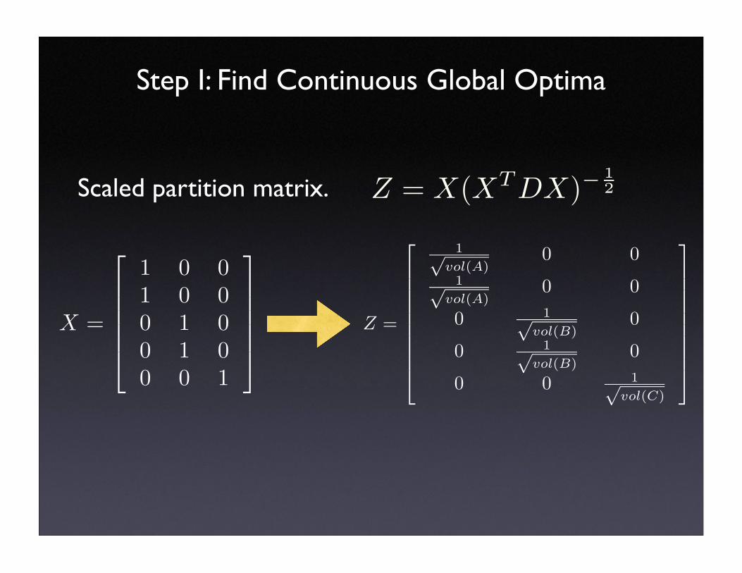
Step I: Find Continuous Global Optima
Z = X(XTDX)−
1
2Scaled partition matrix.
Z =
1√vol(A)
0 0
1√vol(A)
0 0
01√
vol(B)0
01√
vol(B)0
0 01√
vol(C)
X =
1 0 0
1 0 0
0 1 0
0 1 0
0 0 1
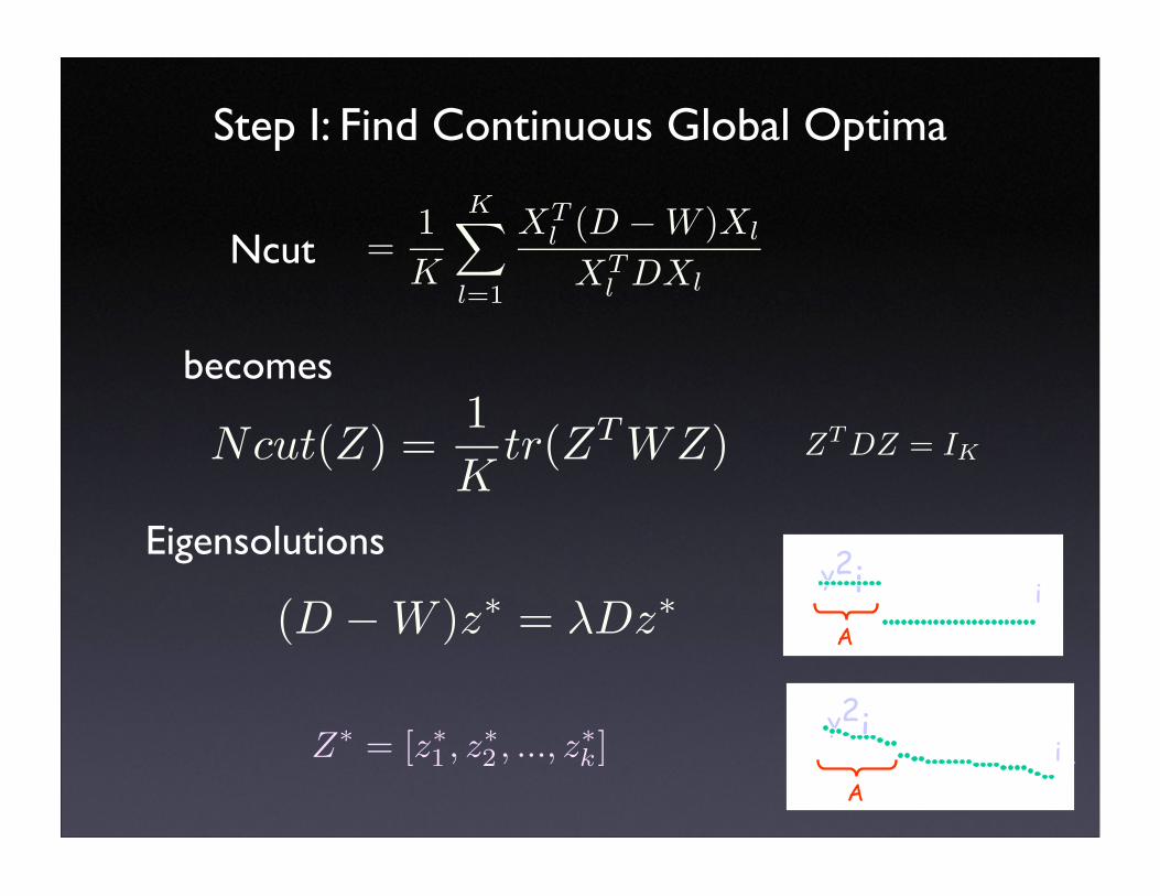
Step I: Find Continuous Global Optima
Ncut(Z) =1
Ktr(ZT
WZ) ZTDZ = IK
becomes
(D − W )z∗ = λDz∗
Eigensolutionsy2i i
A
y2ii
A
=1
K
K∑
l=1
XTl
(D − W )Xl
XTl
DXl
Ncut
Z∗ = [z∗1 , z∗2 , ..., z∗k]
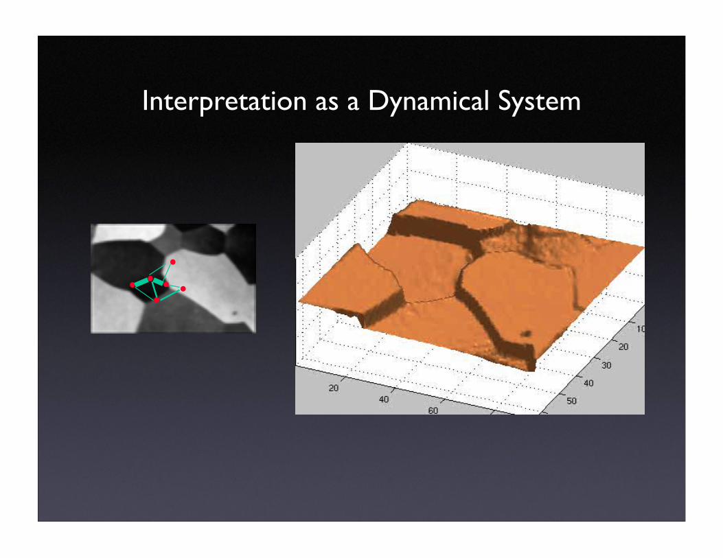
Interpretation as a Dynamical System
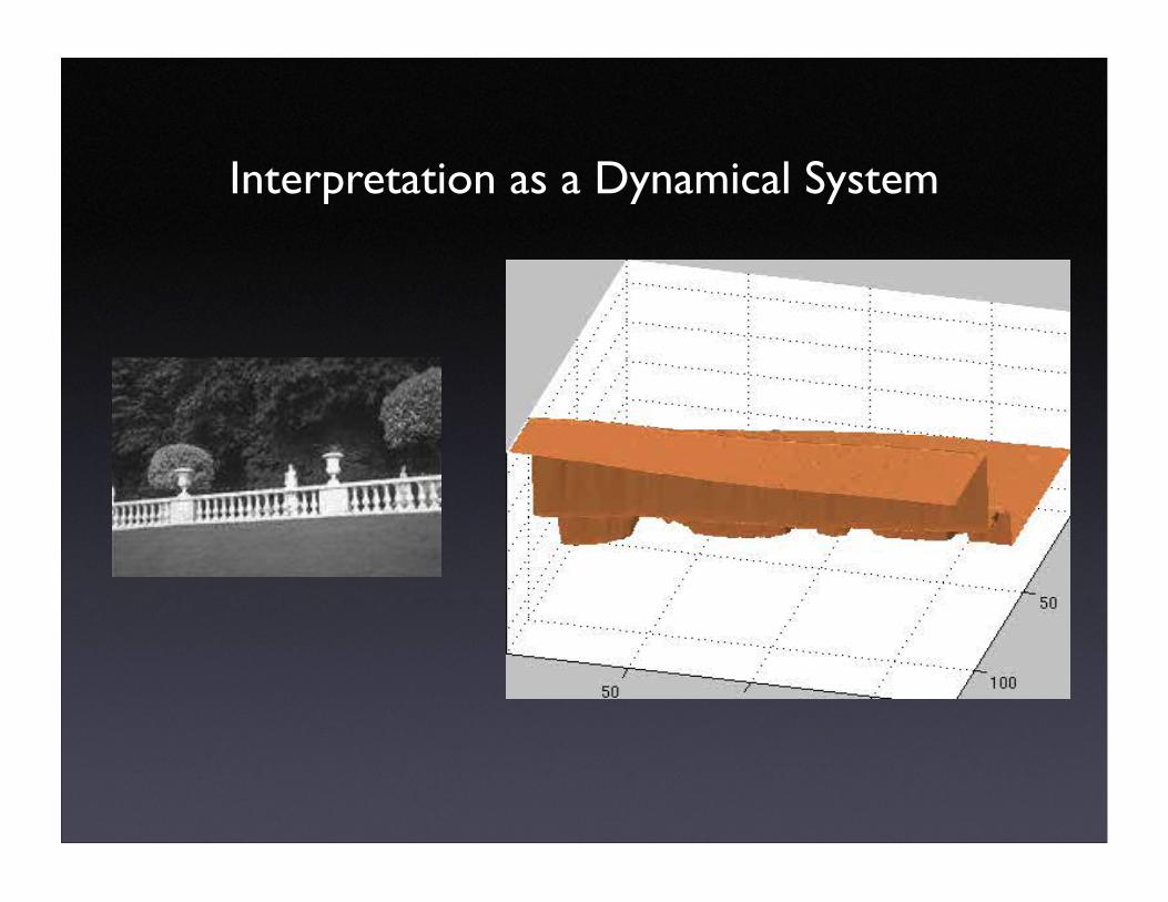
Interpretation as a Dynamical System
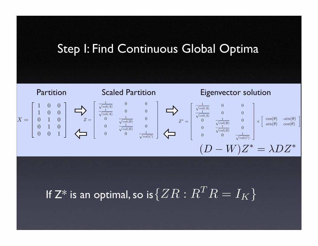
Step I: Find Continuous Global Optima
If Z* is an optimal, so is {ZR : RTR = IK}
Z∗ =
1√vol(A)
0 01√
vol(A)0 0
0 1√vol(B)
0
0 1√vol(B)
0
0 0 1√vol(C)
×
[cos(θ) -sin(θ)sin(θ) cos(θ)
].X =
1 0 0
1 0 0
0 1 0
0 1 0
0 0 1
Partition
Z =
1√vol(A)
0 0
1√vol(A)
0 0
01√
vol(B)0
01√
vol(B)0
0 01√
vol(C)
Scaled Partition Eigenvector solution
(D − W )Z∗ = λDZ∗
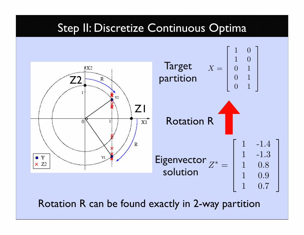
Step II: Discretize Continuous Optima
X =
1 0
1 0
0 1
0 1
0 1
Z1
Z2Target
partition
Z∗
=
1 -1.4
1 -1.3
1 0.8
1 0.9
1 0.7
Eigenvectorsolution
Rotation R
Rotation R can be found exactly in 2-way partition

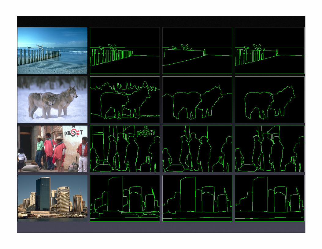
Brightness Image Segmentation
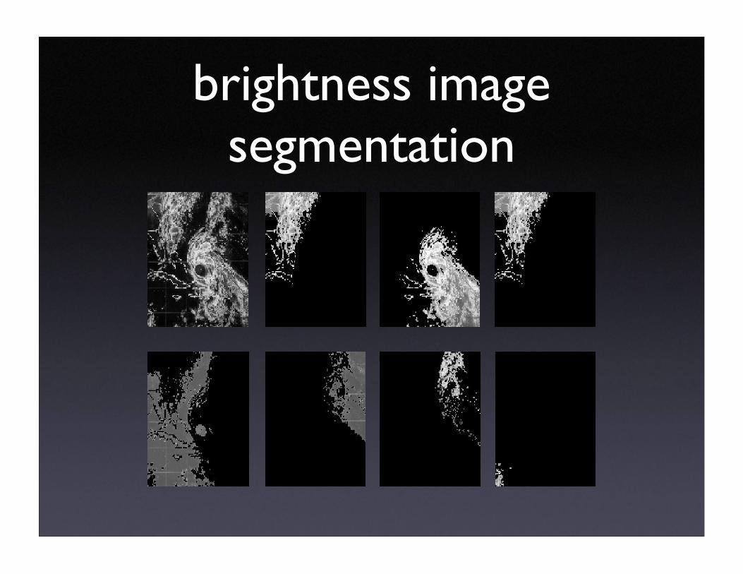
brightness image segmentation

Part II: Segmentation Measurement,
Benchmark


![A robust graph-based segmentation method for breast tumors ... Robust Graph-Based... · Region based segmentation methods based graph theory have also been proposed [21,22]. It is](https://img.pdfslide.us/doc/110x75/601d8da62474fc7d0a5941f9/a-robust-graph-based-segmentation-method-for-breast-tumors-robust-graph-based.jpg)