An Open-Source Version of the Nonpoint Source Pollution and Erosion Comparison Tool

Tutorial for OpenNSPECT, Version 1.1:Example Analyses for the

Waianae Region of Oahu, Hawaii

September 2012

National Oceanic and Atmospheric Administration (NOAA)Coastal Services Center

2234 South Hobson AvenueCharleston, South Carolina 29405-2413

(843) 740-1200www.csc.noaa.gov

Regional Offices:NOAA Pacific Services Center, NOAA Gulf Coast Services Center, andOffices in the Great Lakes, Mid-Atlantic, Northeast, and West Coast

Table of Contents Introduction ............................................................................................................................................ 1 Basic OpenNSPECT Analysis.................................................................................................................... 2

Exercise 1 – Baseline Analysis (Accumulated Effects) ........................................................................ 2 Start MapWindow .......................................................................................................................... 2 Start OpenNSPECT .......................................................................................................................... 2 Set the Analysis Parameters ........................................................................................................... 2 Choose the Analysis Outputs and Run OpenNSPECT ..................................................................... 3 View the Results ............................................................................................................................. 3

Exercise 2 – Baseline Analysis with Local Effects ............................................................................... 4 Rerun OpenNSPECT ........................................................................................................................ 4 View the Results ............................................................................................................................. 5

Advanced OpenNSPECT Analysis – Management Scenario ................................................................... 6

Overview ............................................................................................................................................. 6 Exercise 3 – Analysis with a Management Scenario (Local Effects) ................................................... 7

Select an Area of Interest ............................................................................................................... 7 Start OpenNSPECT and Open a Project .......................................................................................... 8 Run OpenNSPECT ........................................................................................................................... 8 Add a Management Data Layer ...................................................................................................... 9 Start OpenNSPECT and Open a Project ........................................................................................ 10 Apply a Management Scenario .................................................................................................... 11 Run OpenNSPECT ......................................................................................................................... 11 View the Results ........................................................................................................................... 12

Exercise 4 – Compare the Pollutant Yields at the Local Scale (Nitrogen) ......................................... 14 Advanced OpenNSPECT Analysis – Alternative Land Use .................................................................... 16

Overview ........................................................................................................................................... 16 Exercise 5 – Analysis with a New Land Use Scenario (Accumulated Effects) ................................... 16

Add a Land Use Data Layer ........................................................................................................... 17 Run Golf Course Baseline Analysis ................................................................................................ 18 Select Drainage Basins for Processing .......................................................................................... 18 Set Up OpenNSPECT ..................................................................................................................... 18 Analysis Using a Land Use Scenario ............................................................................................. 19 Set Up OpenNSPECT ..................................................................................................................... 19 Add a Land Use Scenario .............................................................................................................. 19 View the Results and Compare to Baseline Data (Nitrogen) ....................................................... 20

Conclusion ............................................................................................................................................ 22 Summary............................................................................................................................................... 22 References ............................................................................................................................................ 22 Acronym List ......................................................................................................................................... 22

1

Tutorial for OpenNSPECT 1.1: Example Analyses for Wai’anae Region of Oahu, Hawai’i

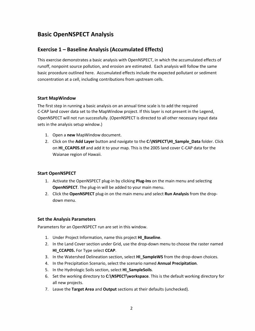
Introduction

OpenNSPECT uses spatial data to simulate the movement and accumulation of water, pollutants, and eroded sediments throughout a watershed. To do this, elevation, land cover, soils, and precipitation data sets are processed to estimate runoff volume, flow direction, and flow accumulation at both the local and watershed levels. Pollutant coefficients, representing the concentration of a pollutant from each land cover class are also applied to approximate total pollutant loads. These coefficients can be taken from published sources or can be derived from local water quality studies. OpenNSPECT output layers display estimates of runoff volume, pollutant loads, pollutant concentration, and total sediment loads. These layers can help resource managers make informed decisions about water quality and about what areas to target for improvement, as well as predict the impacts of management decisions on water quality. OpenNSPECT also provides functionality to compare water quality under current land cover conditions with water quality based on changes proposed to land use and land cover. This tutorial walks the user through a basic run of OpenNSPECT using the provided data. The output data sets from this analysis represent baseline approximations of surface water runoff, erosion caused by surface water runoff, and pollutant mobilization caused by surface water runoff against which past, present, and future land use and land management scenarios can be compared.

Overall Objective:

Run a basic analysis with OpenNSPECT and produce baseline runoff, erosion, and pollutant load data sets for an annual time scale.

Important Learning Objectives:

• Gain familiarity with the OpenNSPECT user interface. • Learn which data sets are necessary to run the model. • Understand the properties associated with the Pollutants tab. • Understand the properties associated with the Erosion tab. • Understand the function of the Local Effects Only option. • Learn to visually assess the data output.

Basic OpenNSPECT Procedure:

1. Start MapWindow. 2. Start OpenNSPECT. 3. Initialize the analysis environment. 4. Choose the analysis outputs in Pollutants and Erosion tabs. 5. Run OpenNSPECT. 6. View the results.

2

Basic OpenNSPECT Analysis

Exercise 1 – Baseline Analysis (Accumulated Effects)

This exercise demonstrates a basic analysis with OpenNSPECT, in which the accumulated effects of runoff, nonpoint source pollution, and erosion are estimated. Each analysis will follow the same basic procedure outlined here. Accumulated effects include the expected pollutant or sediment concentration at a cell, including contributions from upstream cells.

Start MapWindow The first step in running a basic analysis on an annual time scale is to add the required C-CAP land cover data set to the MapWindow project. If this layer is not present in the Legend, OpenNSPECT will not run successfully. (OpenNSPECT is directed to all other necessary input data sets in the analysis setup window.)

1. Open a new MapWindow document. 2. Click on the Add Layer button and navigate to the C:\NSPECT\HI_Sample_Data folder. Click

on HI_CCAP05.tif and add it to your map. This is the 2005 land cover C-CAP data for the Waianae region of Hawaii.

Start OpenNSPECT 1. Activate the OpenNSPECT plug-in by clicking Plug-Ins on the main menu and selecting

OpenNSPECT. The plug-in will be added to your main menu. 2. Click the OpenNSPECT plug-in on the main menu and select Run Analysis from the drop-

down menu.

Set the Analysis Parameters Parameters for an OpenNSPECT run are set in this window.

1. Under Project Information, name this project HI_Baseline. 2. In the Land Cover section under Grid, use the drop-down menu to choose the raster named

HI_CCAP05. For Type select CCAP. 3. In the Watershed Delineation section, select HI_SampleWS from the drop-down choices. 4. In the Precipitation Scenario, select the scenario named Annual Precipitation. 5. In the Hydrologic Soils section, select HI_SampleSoils. 6. Set the working directory to C:\NSPECT\workspace. This is the default working directory for

all new projects. 7. Leave the Target Area and Output sections at their defaults (unchecked).

3

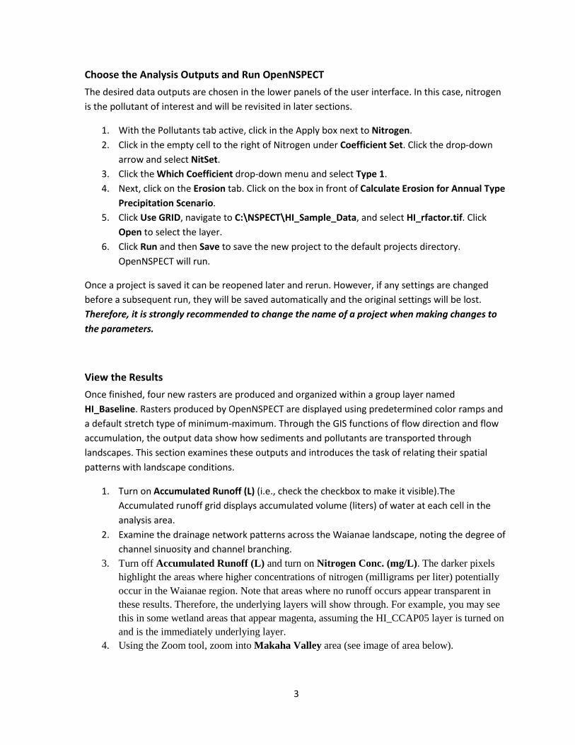
Choose the Analysis Outputs and Run OpenNSPECT The desired data outputs are chosen in the lower panels of the user interface. In this case, nitrogen is the pollutant of interest and will be revisited in later sections.

1. With the Pollutants tab active, click in the Apply box next to Nitrogen. 2. Click in the empty cell to the right of Nitrogen under Coefficient Set. Click the drop-down

arrow and select NitSet. 3. Click the Which Coefficient drop-down menu and select Type 1. 4. Next, click on the Erosion tab. Click on the box in front of Calculate Erosion for Annual Type

Precipitation Scenario. 5. Click Use GRID, navigate to C:\NSPECT\HI_Sample_Data, and select HI_rfactor.tif. Click

Open to select the layer. 6. Click Run and then Save to save the new project to the default projects directory.

OpenNSPECT will run.

Once a project is saved it can be reopened later and rerun. However, if any settings are changed before a subsequent run, they will be saved automatically and the original settings will be lost. Therefore, it is strongly recommended to change the name of a project when making changes to the parameters.

View the Results Once finished, four new rasters are produced and organized within a group layer named HI_Baseline. Rasters produced by OpenNSPECT are displayed using predetermined color ramps and a default stretch type of minimum-maximum. Through the GIS functions of flow direction and flow accumulation, the output data show how sediments and pollutants are transported through landscapes. This section examines these outputs and introduces the task of relating their spatial patterns with landscape conditions.

1. Turn on Accumulated Runoff (L) (i.e., check the checkbox to make it visible).The Accumulated runoff grid displays accumulated volume (liters) of water at each cell in the analysis area.

2. Examine the drainage network patterns across the Waianae landscape, noting the degree of channel sinuosity and channel branching.

3. Turn off Accumulated Runoff (L) and turn on Nitrogen Conc. (mg/L). The darker pixels highlight the areas where higher concentrations of nitrogen (milligrams per liter) potentially occur in the Waianae region. Note that areas where no runoff occurs appear transparent in these results. Therefore, the underlying layers will show through. For example, you may see this in some wetland areas that appear magenta, assuming the HI_CCAP05 layer is turned on and is the immediately underlying layer.

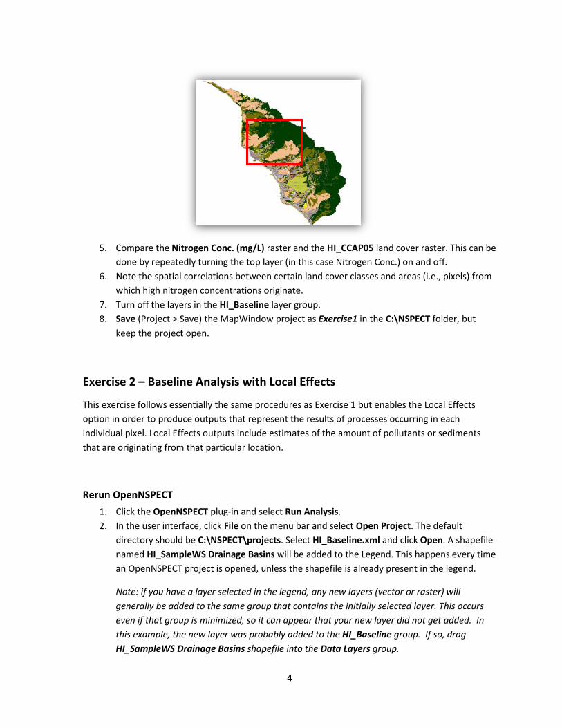
4. Using the Zoom tool, zoom into Makaha Valley area (see image of area below).

4

5. Compare the Nitrogen Conc. (mg/L) raster and the HI_CCAP05 land cover raster. This can be

done by repeatedly turning the top layer (in this case Nitrogen Conc.) on and off. 6. Note the spatial correlations between certain land cover classes and areas (i.e., pixels) from

which high nitrogen concentrations originate. 7. Turn off the layers in the HI_Baseline layer group. 8. Save (Project > Save) the MapWindow project as Exercise1 in the C:\NSPECT folder, but

keep the project open.

Exercise 2 – Baseline Analysis with Local Effects

This exercise follows essentially the same procedures as Exercise 1 but enables the Local Effects option in order to produce outputs that represent the results of processes occurring in each individual pixel. Local Effects outputs include estimates of the amount of pollutants or sediments that are originating from that particular location.

Rerun OpenNSPECT 1. Click the OpenNSPECT plug-in and select Run Analysis. 2. In the user interface, click File on the menu bar and select Open Project. The default

directory should be C:\NSPECT\projects. Select HI_Baseline.xml and click Open. A shapefile named HI_SampleWS Drainage Basins will be added to the Legend. This happens every time an OpenNSPECT project is opened, unless the shapefile is already present in the legend.

Note: if you have a layer selected in the legend, any new layers (vector or raster) will generally be added to the same group that contains the initially selected layer. This occurs even if that group is minimized, so it can appear that your new layer did not get added. In this example, the new layer was probably added to the HI_Baseline group. If so, drag HI_SampleWS Drainage Basins shapefile into the Data Layers group.

5

3. Change the name in the Project Information section to HI_Baseline_LE. 4. In the Output section, click the check box next to Include Local Effects. 5. Click Run. 6. A window will appear that notifies the user that the project name has changed. Click Yes

and save the new project file as HI_Baseline_LE. 7. Click Save. Wait while OpenNSPECT runs.

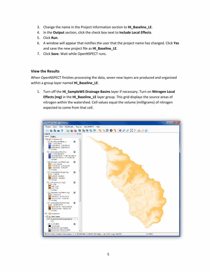
View the Results When OpenNSPECT finishes processing the data, seven new layers are produced and organized within a group layer named HI_Baseline_LE.

1. Turn off the HI_SampleWS Drainage Basins layer if necessary. Turn on Nitrogen Local Effects (mg) in the HI_Baseline_LE layer group. This grid displays the source areas of nitrogen within the watershed. Cell values equal the volume (milligrams) of nitrogen expected to come from that cell.

6

2. Click the Add Layers button, navigate to the C:\NSPECT\HI_Sample_Data folder, and add the files HI_dem_30.tif and HI_annual_prec.tif to your map Note: MapWindow may add the layers into different Data Groups when adding multiple files simultaneously. You may want to organize (drag and drop) the HI_annual_prec, HI_dem_30, and HI_SampleWS Drainage Basins layers into one Data Group to keep your map organized.

3. Zoom back in to the Makaha Valley area. Compare the areas producing high amounts of nitrogen to the land cover, precipitation, and elevation data sets.

4. Save the MapWindow project as Exercise2 (Project > Save As), but do not exit.

Advanced OpenNSPECT Analysis – Management Scenario

Overview

This section explores using the land management scenario feature to illustrate the flexibility and decision-support functionality offered by OpenNSPECT. OpenNSPECT has the capability to incorporate a polygon shapefile, representing a management area that differs from the existing land cover data, into an analysis in order to study its impacts on nonpoint-source pollution and erosion. The user will define an area that will change from its existing land cover state to a different, single land cover class in order to study the effects of an alternative land use. For this function to work, this alternate land use type must be within the predefined land cover types and be fully parameterized with pollutant coefficients, a curve number, and a cover factor.

The spatial focus of this exercise narrows from the entire Waianae region to Makaha Valley. Of all the areas within the Waianae region, the Department of Planning and Permitting attributed this watershed with a “Special Area Plan” status to devote more attention to planning and guiding development (City and County of Honolulu, 2000). One of the reasons for this designation was that several hundred acres of land were undeveloped but zoned for residential and resort uses. The valley was also recognized as an important resource area in terms of water resources, rare and endangered plants and animals, and cultural sites.

In this exercise, OpenNSPECT will help the user predict changes to runoff, erosion, and nonpoint source pollution caused by a proposed land use change by superimposing a hypothetical low-intensity development upon the existing land cover data. The outline below describes the general process the user will follow.

7

Overall Objective:

Run an analysis that incorporates a hypothetical management scenario and examines the potential changes to runoff, erosion, and pollution.

Important Learning Objectives:

• Understand the properties associated with the Management Scenarios tab. • Learn to incorporate a management scenario. • Learn to quantitatively evaluate the data output. • Understand the relative contributions of different land cover classes to nonpoint

source pollution.

Advanced OpenNSPECT Procedure:

1. Add a management scenario (polygon shapefile) to MapWindow. 2. Start OpenNSPECT and open an existing project. 3. Select the management scenario and set the new land use class. 4. Run OpenNSPECT and examine the results.

Exercise 3 – Analysis with a Management Scenario (Local Effects)

This exercise incorporates a hypothetical management scenario in the analysis of nonpoint source pollution and erosion and seeks to illustrate the local effects of such a land cover change. This exercise also illustrates the use of the Selected Polygons Only feature by constraining the OpenNSPECT analysis to the largest portion of Makaha Valley. The management scenario accumulated effects will also be analyzed and compared to the local effects results.

Select an Area of Interest 1. In your Exercise 2 project turn off all data layers except HI_SampleWS Drainage Basins.

Double-click the drainage basins layer, click the Appearance tab, locate Transparency and move it to 125 (60%). Select the More Options button, click on the Outline tab and change the color to red (double-click). Set the transparency level for the outline to 255. Click OK twice to exit the Symbology editor.

2. In the Legend place the HI_dem_30 layer directly beneath the HI_SampleWS Drainage Basins layer. You should now see the drainage basins layer draped over the hill-shaded DEM.

8

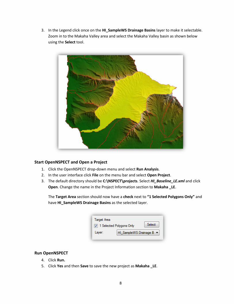
3. In the Legend click once on the HI_SampleWS Drainage Basins layer to make it selectable. Zoom in to the Makaha Valley area and select the Makaha Valley basin as shown below using the Select tool.

Start OpenNSPECT and Open a Project 1. Click the OpenNSPECT drop-down menu and select Run Analysis. 2. In the user interface click File on the menu bar and select Open Project. 3. The default directory should be C:\NSPECT\projects. Select HI_Baseline_LE.xml and click

Open. Change the name in the Project Information section to Makaha _LE.

The Target Area section should now have a check next to “1 Selected Polygons Only” and have HI_SampleWS Drainage Basins as the selected layer.

Run OpenNSPECT 4. Click Run. 5. Click Yes and then Save to save the new project as Makaha _LE.

9

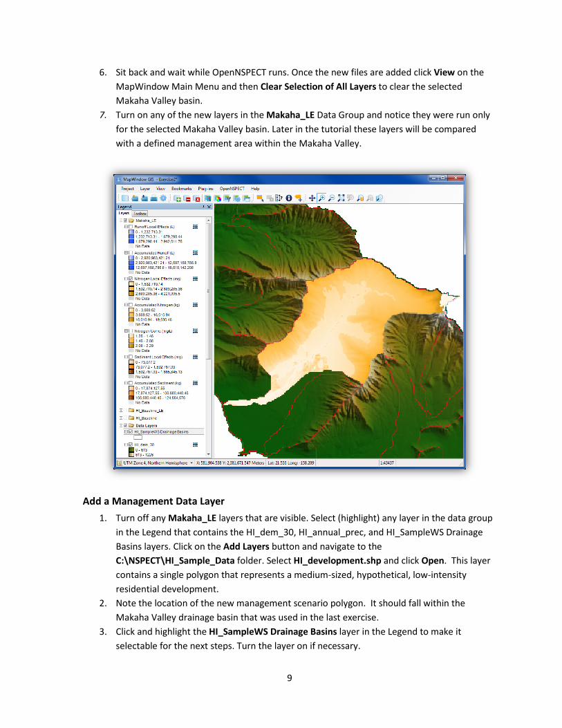
6. Sit back and wait while OpenNSPECT runs. Once the new files are added click View on the MapWindow Main Menu and then Clear Selection of All Layers to clear the selected Makaha Valley basin.

7. Turn on any of the new layers in the Makaha_LE Data Group and notice they were run only for the selected Makaha Valley basin. Later in the tutorial these layers will be compared with a defined management area within the Makaha Valley.

Add a Management Data Layer 1. Turn off any Makaha_LE layers that are visible. Select (highlight) any layer in the data group

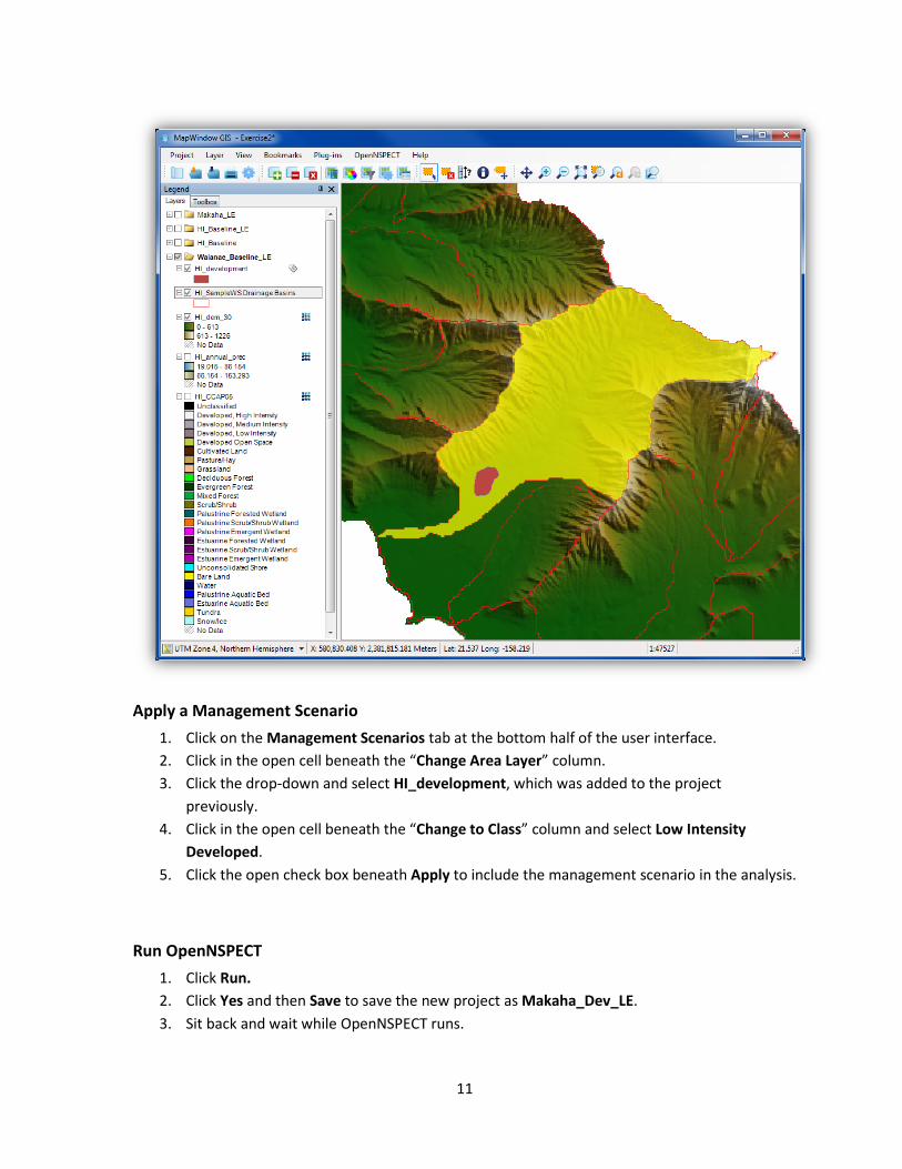
in the Legend that contains the HI_dem_30, HI_annual_prec, and HI_SampleWS Drainage Basins layers. Click on the Add Layers button and navigate to the C:\NSPECT\HI_Sample_Data folder. Select HI_development.shp and click Open. This layer contains a single polygon that represents a medium-sized, hypothetical, low-intensity residential development.

2. Note the location of the new management scenario polygon. It should fall within the Makaha Valley drainage basin that was used in the last exercise.

3. Click and highlight the HI_SampleWS Drainage Basins layer in the Legend to make it selectable for the next steps. Turn the layer on if necessary.

10

Start OpenNSPECT and Open a Project 1. Click the OpenNSPECT drop-down menu and select Run Analysis. 2. In the user interface, click File on the menu bar and select Open Project. 3. The default directory should be C:\OpenNSPECT\Projects. Select Makaha _LE.xml and click

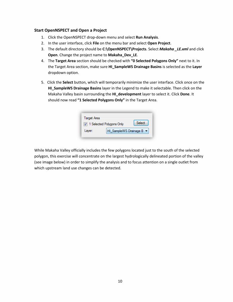
Open. Change the project name to Makaha_Dev_LE. 4. The Target Area section should be checked with “0 Selected Polygons Only” next to it. In

the Target Area section, make sure HI_SampleWS Drainage Basins is selected as the Layer dropdown option.

5. Click the Select button, which will temporarily minimize the user interface. Click once on the HI_SampleWS Drainage Basins layer in the Legend to make it selectable. Then click on the Makaha Valley basin surrounding the HI_development layer to select it. Click Done. It should now read “1 Selected Polygons Only” in the Target Area.

While Makaha Valley officially includes the few polygons located just to the south of the selected polygon, this exercise will concentrate on the largest hydrologically delineated portion of the valley (see image below) in order to simplify the analysis and to focus attention on a single outlet from which upstream land use changes can be detected.

11

Apply a Management Scenario 1. Click on the Management Scenarios tab at the bottom half of the user interface. 2. Click in the open cell beneath the “Change Area Layer” column. 3. Click the drop-down and select HI_development, which was added to the project

previously. 4. Click in the open cell beneath the “Change to Class” column and select Low Intensity

Developed. 5. Click the open check box beneath Apply to include the management scenario in the analysis.

Run OpenNSPECT 1. Click Run. 2. Click Yes and then Save to save the new project as Makaha_Dev_LE. 3. Sit back and wait while OpenNSPECT runs.

12

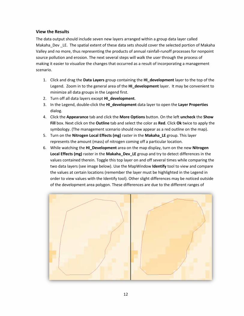
View the Results The data output should include seven new layers arranged within a group data layer called Makaha_Dev _LE. The spatial extent of these data sets should cover the selected portion of Makaha Valley and no more, thus representing the products of annual rainfall-runoff processes for nonpoint source pollution and erosion. The next several steps will walk the user through the process of making it easier to visualize the changes that occurred as a result of incorporating a management scenario.

1. Click and drag the Data Layers group containing the HI_development layer to the top of the Legend. Zoom in to the general area of the HI_development layer. It may be convenient to minimize all data groups in the Legend first.

2. Turn off all data layers except HI_development. 3. In the Legend, double-click the HI_development data layer to open the Layer Properties

dialog. 4. Click the Appearance tab and click the More Options button. On the left uncheck the Show

Fill box. Next click on the Outline tab and select the color as Red. Click Ok twice to apply the symbology. (The management scenario should now appear as a red outline on the map).

5. Turn on the Nitrogen Local Effects (mg) raster in the Makaha_LE group. This layer represents the amount (mass) of nitrogen coming off a particular location.

6. While watching the HI_Development area on the map display, turn on the new Nitrogen Local Effects (mg) raster in the Makaha_Dev_LE group and try to detect differences in the values contained therein. Toggle this top layer on and off several times while comparing the two data layers (see image below). Use the MapWindow Identify tool to view and compare the values at certain locations (remember the layer must be highlighted in the Legend in order to view values with the Identify tool). Other slight differences may be noticed outside of the development area polygon. These differences are due to the different ranges of

13

symbolized values contained in the two rasters. 7. Repeat steps 5 and 6 for Runoff Local Effects (L) and Sediment Local Effects (mg). 8. When finished comparing the local effects scenarios turn them off and turn on the

Accumulated Runoff (L) layers in both the Makaha_Dev_LE and Makaha_LE layer groups. These layers represent the amount (mass) of runoff delivered to/through a location for the given analysis.

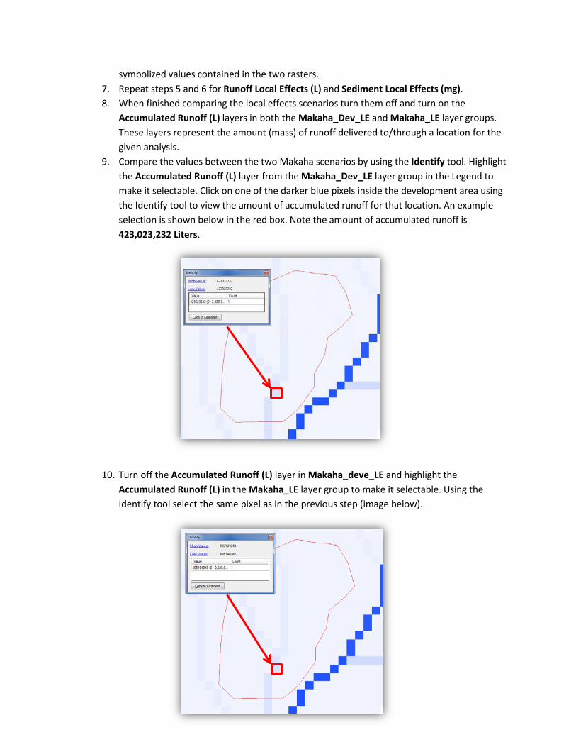
9. Compare the values between the two Makaha scenarios by using the Identify tool. Highlight the Accumulated Runoff (L) layer from the Makaha_Dev_LE layer group in the Legend to make it selectable. Click on one of the darker blue pixels inside the development area using the Identify tool to view the amount of accumulated runoff for that location. An example selection is shown below in the red box. Note the amount of accumulated runoff is 423,023,232 Liters.

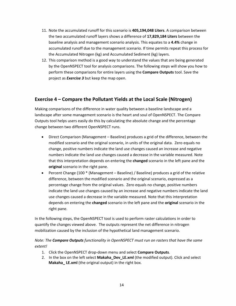
10. Turn off the Accumulated Runoff (L) layer in Makaha_deve_LE and highlight the

Accumulated Runoff (L) in the Makaha_LE layer group to make it selectable. Using the Identify tool select the same pixel as in the previous step (image below).

14

11. Note the accumulated runoff for this scenario is 405,194,048 Liters. A comparison between the two accumulated runoff layers shows a difference of 17,829,184 Liters between the baseline analysis and management scenario analysis. This equates to a 4.4% change in accumulated runoff due to the management scenario. If time permits repeat this process for the Accumulated Nitrogen (kg) and Accumulated Sediment (kg) layers.

12. This comparison method is a good way to understand the values that are being generated by the OpenNSPECT tool for analysis comparisons. The following steps will show you how to perform these comparisons for entire layers using the Compare Outputs tool. Save the project as Exercise 3 but keep the map open.

Exercise 4 – Compare the Pollutant Yields at the Local Scale (Nitrogen)

Making comparisons of the difference in water quality between a baseline landscape and a landscape after some management scenario is the heart and soul of OpenNSPECT. The Compare Outputs tool helps users easily do this by calculating the absolute change and the percentage change between two different OpenNSPECT runs.

• Direct Comparison (Management – Baseline) produces a grid of the difference, between the modified scenario and the original scenario, in units of the original data. Zero equals no change, positive numbers indicate the land use changes caused an increase and negative numbers indicate the land use changes caused a decrease in the variable measured. Note that this interpretation depends on entering the changed scenario in the left pane and the original scenario in the right pane.

• Percent Change (100 * (Management – Baseline) / Baseline) produces a grid of the relative difference, between the modified scenario and the original scenario, expressed as a percentage change from the original values. Zero equals no change, positive numbers indicate the land use changes caused by an increase and negative numbers indicate the land use changes caused a decrease in the variable measured. Note that this interpretation depends on entering the changed scenario in the left pane and the original scenario in the right pane.

In the following steps, the OpenNSPECT tool is used to perform raster calculations in order to quantify the changes viewed above. The outputs represent the net difference in nitrogen mobilization caused by the inclusion of the hypothetical land management scenario.

Note: The Compare Outputs functionality in OpenNSPECT must run on rasters that have the same extent!

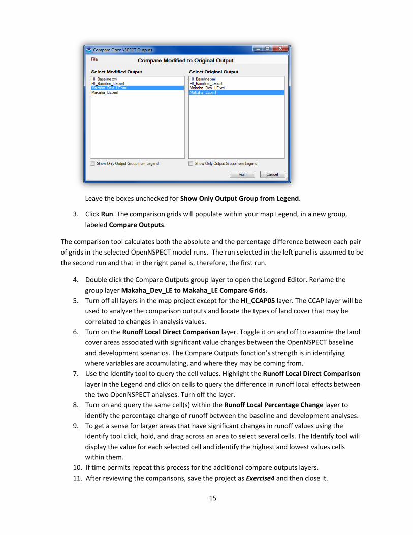
1. Click the OpenNSPECT drop-down menu and select Compare Outputs. 2. In the box on the left select Makaha_Dev_LE.xml (the modified output). Click and select

Makaha_ LE.xml (the original output) in the right box.

15

Leave the boxes unchecked for Show Only Output Group from Legend.

3. Click Run. The comparison grids will populate within your map Legend, in a new group, labeled Compare Outputs.

The comparison tool calculates both the absolute and the percentage difference between each pair of grids in the selected OpenNSPECT model runs. The run selected in the left panel is assumed to be the second run and that in the right panel is, therefore, the first run.

4. Double click the Compare Outputs group layer to open the Legend Editor. Rename the group layer Makaha_Dev_LE to Makaha_LE Compare Grids.

5. Turn off all layers in the map project except for the HI_CCAP05 layer. The CCAP layer will be used to analyze the comparison outputs and locate the types of land cover that may be correlated to changes in analysis values.

6. Turn on the Runoff Local Direct Comparison layer. Toggle it on and off to examine the land cover areas associated with significant value changes between the OpenNSPECT baseline and development scenarios. The Compare Outputs function’s strength is in identifying where variables are accumulating, and where they may be coming from.

7. Use the Identify tool to query the cell values. Highlight the Runoff Local Direct Comparison layer in the Legend and click on cells to query the difference in runoff local effects between the two OpenNSPECT analyses. Turn off the layer.

8. Turn on and query the same cell(s) within the Runoff Local Percentage Change layer to identify the percentage change of runoff between the baseline and development analyses.

9. To get a sense for larger areas that have significant changes in runoff values using the Identify tool click, hold, and drag across an area to select several cells. The Identify tool will display the value for each selected cell and identify the highest and lowest values cells within them.

10. If time permits repeat this process for the additional compare outputs layers. 11. After reviewing the comparisons, save the project as Exercise4 and then close it.

16

Advanced OpenNSPECT Analysis – Alternative Land Use

Overview

This section expands upon the previous section by incorporating an alternative land use scenario in order to further illustrate the flexibility and decision support functionality offered by OpenNSPECT. The user will create a new land use scenario with customized pollutant coefficients in order to study the effects of changes to land cover and land use.

The current version of OpenNSPECT with the original C-CAP data does not distinguish between the three classes mentioned above, yet each class clearly impacts nonpoint source pollution and erosion differently. This exercise uses the land use tab to allow the user to add a new land use scenario complete with new coefficients that more accurately reflect the underlying conditions of the selected layer. In this case, a shapefile will be added to the project that covers the area of two existing golf courses in Makaha Valley, and new coefficients will be defined for this type of land use.

Overall Objective:

Run an analysis with a customized land use scenario and produce modified runoff, erosion, and pollutant load data sets for an annual time scale.

Important Learning Objectives:

• Understand the properties associated with the Land Use tab. • Learn to parameterize a new land use scenario. • Learn to quantitatively evaluate the data output.

Advanced OpenNSPECT Procedure:

1. Start OpenNSPECT and open an existing project. 2. Add a new land use scenario and define the new coefficients. 3. Run OpenNSPECT and examine the results.

Exercise 5 – Analysis with a New Land Use Scenario (Accumulated Effects)

This exercise incorporates a land use scenario in the analysis of nonpoint source pollution and erosion and seeks to illustrate the accumulated effects of spatially delineating an area with unique land cover characteristics. In this case, the Makaha Valley Country Club and the Makaha Resort Golf Club were hand-digitized from a high resolution satellite image of the Waianae region.

17

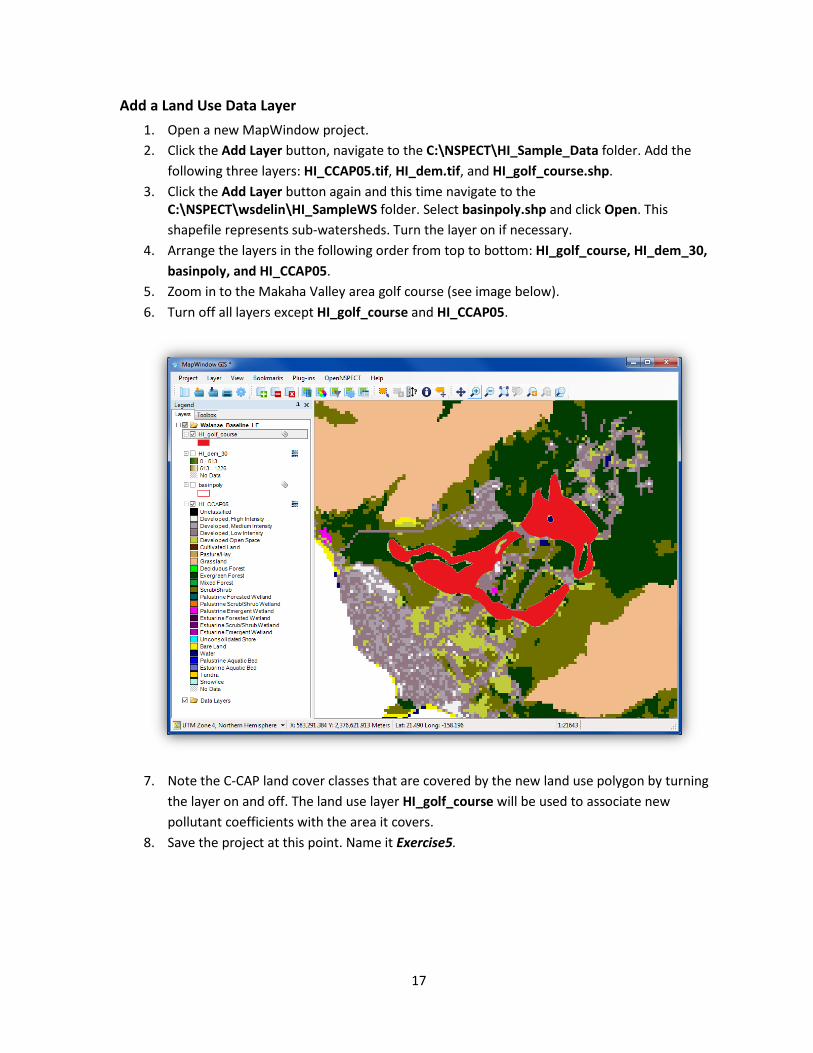
Add a Land Use Data Layer 1. Open a new MapWindow project. 2. Click the Add Layer button, navigate to the C:\NSPECT\HI_Sample_Data folder. Add the

following three layers: HI_CCAP05.tif, HI_dem.tif, and HI_golf_course.shp. 3. Click the Add Layer button again and this time navigate to the

C:\NSPECT\wsdelin\HI_SampleWS folder. Select basinpoly.shp and click Open. This shapefile represents sub-watersheds. Turn the layer on if necessary.

4. Arrange the layers in the following order from top to bottom: HI_golf_course, HI_dem_30, basinpoly, and HI_CCAP05.

5. Zoom in to the Makaha Valley area golf course (see image below). 6. Turn off all layers except HI_golf_course and HI_CCAP05.

7. Note the C-CAP land cover classes that are covered by the new land use polygon by turning the layer on and off. The land use layer HI_golf_course will be used to associate new pollutant coefficients with the area it covers.

8. Save the project at this point. Name it Exercise5.

18

Run Golf Course Baseline Analysis

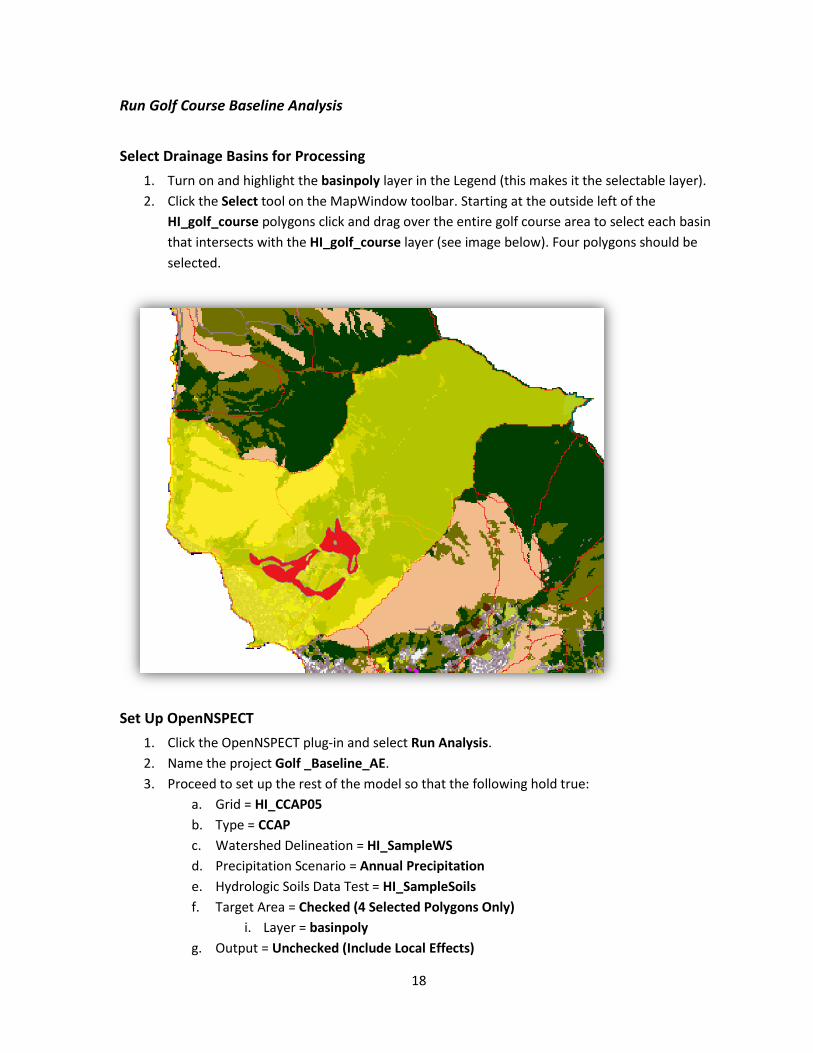
Select Drainage Basins for Processing 1. Turn on and highlight the basinpoly layer in the Legend (this makes it the selectable layer). 2. Click the Select tool on the MapWindow toolbar. Starting at the outside left of the

HI_golf_course polygons click and drag over the entire golf course area to select each basin that intersects with the HI_golf_course layer (see image below). Four polygons should be selected.

Set Up OpenNSPECT 1. Click the OpenNSPECT plug-in and select Run Analysis. 2. Name the project Golf _Baseline_AE. 3. Proceed to set up the rest of the model so that the following hold true:

a. Grid = HI_CCAP05 b. Type = CCAP c. Watershed Delineation = HI_SampleWS d. Precipitation Scenario = Annual Precipitation e. Hydrologic Soils Data Test = HI_SampleSoils f. Target Area = Checked (4 Selected Polygons Only)

i. Layer = basinpoly g. Output = Unchecked (Include Local Effects)

19

h. Working Directory = C:\NSPECT\workspace i. Pollutants =

i. Phosphorus, PhosSet, Type 1 ii. Nitrogen, NitSet, Type 1

iii. Check the Apply check box for both pollutants j. On the Erosion tab: Check the Calculate Erosion... check box and select and set the

Use Grid to C:\NSPECT\HI_Sample_Data\HI_rfactor.tif. 4. Click Run. Click Yes and save the new project as Golf_Baseline_AE. Wait while OpenNSPECT

processes the new scenario.

Six new raster layers are added to your map. These baseline runs for the Makaha Valley basin will be used to compare the land use scenario layers you will create in the next steps.

Analysis Using a Land Use Scenario

Set Up OpenNSPECT 1. Select the OpenNSPECT plug-in again and select Run Analysis. 2. Click File Open and select Golf_Baseline_AE. Click Open. 3. Change the name of the project to Golf _LandUse_AE. 4. In the Target Area section select the Target layer as basinpoly (The basinpoly layer

must be highlighted in the map Legend to be selectable). 5. Click the Select button in Target Area. The Target Area section should now say “4

Selected Polygons Only.”

Add a Land Use Scenario 1. Click the Land Uses tab. 2. Right-click anywhere below the Land Use Scenario column and click Add Scenario. 3. Name the scenario Golf Course. Select HI_golf_course from the Layer option. 4. Leave the check box for Use Selected Polygons Only blank. This option could be enabled if

the scenario shapefile held multiple polygons of which one or a few were selected for land use changes.

5. Enter the following values in the SCS curve number cells:

A B C D

0.39 0.61 0.74 0.80

20

These factors represent the infiltration capacity of the soil and range from 0.00 (0%) to 1.00 (100%), with 0.00 being no runoff and 1.00 indicating no infiltration. The categories A through D represent four hydrologic soil types, again relating to infiltration capacity where soil type A has a higher infiltration capacity than soil type D. Curve numbers play an important role in runoff depth estimation calculations. The values used in this example are the same as those included in OpenNSPECT for the C-CAP grassland land cover class. If different values are known to represent a certain land use better than those included with OpenNSPECT, then this dialog box is where they can be entered.

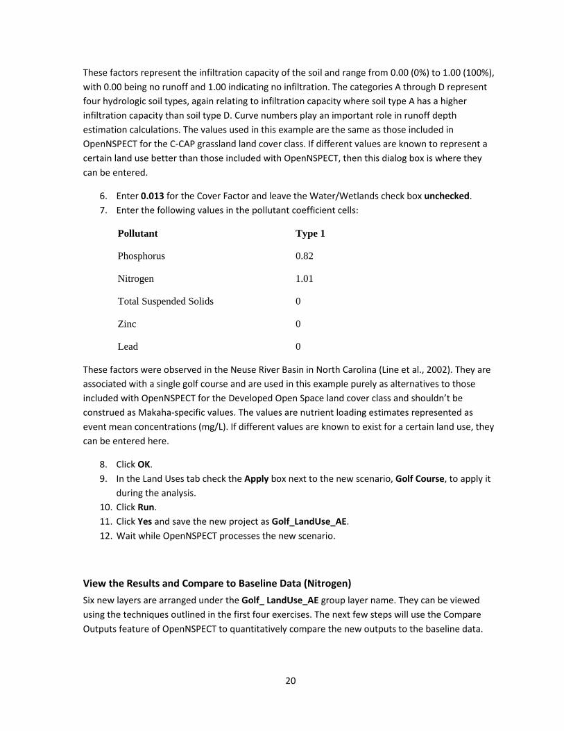
6. Enter 0.013 for the Cover Factor and leave the Water/Wetlands check box unchecked. 7. Enter the following values in the pollutant coefficient cells:

Pollutant Type 1

Phosphorus 0.82

Nitrogen 1.01

Total Suspended Solids 0

Zinc 0

Lead 0

These factors were observed in the Neuse River Basin in North Carolina (Line et al., 2002). They are associated with a single golf course and are used in this example purely as alternatives to those included with OpenNSPECT for the Developed Open Space land cover class and shouldn’t be construed as Makaha-specific values. The values are nutrient loading estimates represented as event mean concentrations (mg/L). If different values are known to exist for a certain land use, they can be entered here.

8. Click OK. 9. In the Land Uses tab check the Apply box next to the new scenario, Golf Course, to apply it

during the analysis. 10. Click Run. 11. Click Yes and save the new project as Golf_LandUse_AE. 12. Wait while OpenNSPECT processes the new scenario.

View the Results and Compare to Baseline Data (Nitrogen) Six new layers are arranged under the Golf_ LandUse_AE group layer name. They can be viewed using the techniques outlined in the first four exercises. The next few steps will use the Compare Outputs feature of OpenNSPECT to quantitatively compare the new outputs to the baseline data.

21

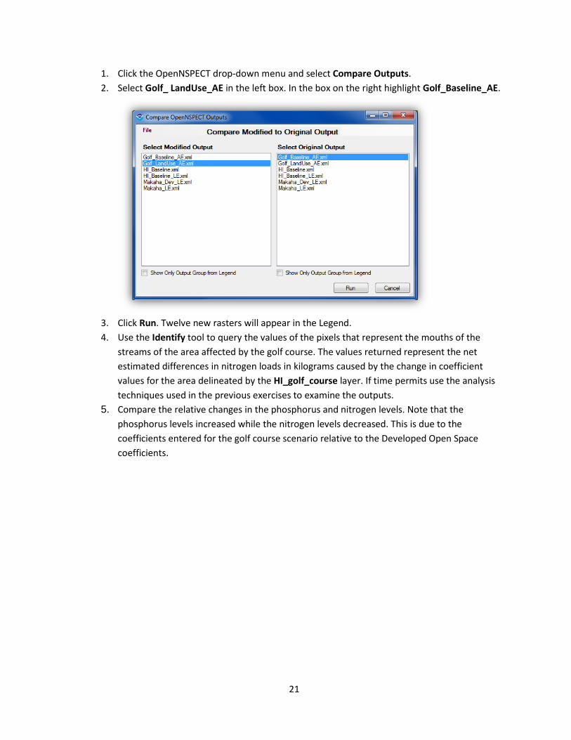
1. Click the OpenNSPECT drop-down menu and select Compare Outputs. 2. Select Golf_ LandUse_AE in the left box. In the box on the right highlight Golf_Baseline_AE.

3. Click Run. Twelve new rasters will appear in the Legend. 4. Use the Identify tool to query the values of the pixels that represent the mouths of the

streams of the area affected by the golf course. The values returned represent the net estimated differences in nitrogen loads in kilograms caused by the change in coefficient values for the area delineated by the HI_golf_course layer. If time permits use the analysis techniques used in the previous exercises to examine the outputs.

5. Compare the relative changes in the phosphorus and nitrogen levels. Note that the phosphorus levels increased while the nitrogen levels decreased. This is due to the coefficients entered for the golf course scenario relative to the Developed Open Space coefficients.

22

Conclusion

This exercise illustrated the changes to OpenNSPECT outputs that accompany the inclusion of an alternative land use scenario. In this case, the land use feature was used to force OpenNSPECT to incorporate a unique land use that is not adequately represented by the original C-CAP land cover classification scheme. With proper data preparation, the land use scenario feature can be used to address other land use issues that would benefit from user defined pollutant coefficients, curve numbers, and cover factors.

Summary

Users have now used OpenNSPECT to conduct a baseline run, to simulate results of management and land use changes and analyze the impacts of these changes using sample data. To perform similar analyses with their own data, the users will need to refer to the Advanced Options under the OpenNSPECT menu. There they will find options for using custom land cover, nutrients, soils, and watersheds. For more information on using these advanced options please visit the OpenNSPECT homepage (csc.noaa.gov/nspect).

References

City and County of Honolulu. 2000. "Waianae Sustainable Communities Plan." Department of Planning and Permitting. Honolulu, HI.

Line, D.E., N.M. White, D.L. Osmond, G.D. Jennings, and C.B. Mojonnier. 2002. “Pollutant Export from Various Land Uses in the Upper Neuse River Basin.” Water Environment Research. Volume 74, Number 1. Pages 100 to 108.

Acronym List

C-CAP: Coastal-Change Analysis Program DEM: Digital Elevation Model EMC: Event Mean Concentration MUSLE: Modified Universal Soil Loss Equation NRCS: Natural Resources Conservation Service NSPECT: Nonpoint Source Pollution and Erosion Comparison Tool NWS: National Weather Service RUSLE: Revised Universal Soil Loss Equation SCS Curve Number: Soil Conservation Service Curve Number SSURGO Database: Soil Survey Geographic Database USDA: United States Department of Agriculture USGS: United States Geological Survey