1  

Tutorial examples for uncertainty quantification methods

Sarah de Bord

Mathematics, UC Davis, Davis, California 95616-0009, USA

This report details the work accomplished during my 2015 SULI summer

internship at Sandia National Laboratories in Livermore, CA. During this

internship, I worked on multiple tasks with the common goal of making

uncertainty quantification (UQ) methods more accessible to the general

scientific community. As part of my work, I created a comprehensive

numerical integration example to incorporate into the user manual of a UQ

software package. Further, I developed examples involving heat transfer

through a window to incorporate into tutorial lectures that serve as an

introduction to UQ methods.

I. INTRODUCTION

My work during my SULI internship this summer consisted of several different

projects, all with the goal of making uncertainty quantification tools accessible to a wider

audience. The term uncertainty quantification (UQ) covers a wide variety of methods, but

in a broad sense these are methods to enable predictive simulations by assessing all

sources of uncertainty in computational models. These methods are useful across many

disciplines, as predictive simulations are necessary when experiments are costly or

SAND2015-7083R

 2  

otherwise unfeasible3. To complete my projects, I used software developed at Sandia

known as the UQ Toolkit (UQTk). UQTk is a collection of tools and libraries that can be

used to quantify uncertainty in numerical model predictions. It is released as a C++ open

source library and is available for download at http://www.sandia.gov/uqtoolkit/6. My

initial task was to create a tutorial for the user manual on how to use UQTk to perform

numerical integrations. Next, I created an example involving heat transfer through a

window to include in a tutorial lecture on the fundamentals of UQ. Finally, I worked on

expanding the window heat transfer example to include radiative heat transfer.

II. UQTk MANUAL NUMERICAL INTEGRATION EXAMPLE

My main task this summer was creating a tutorial on how to use the Python

interface of UQTk to perform numerical integrations. This tutorial was then incorporated

into the UQTk user manual. It is crucial for user manuals to contain comprehensive and

interactive examples, especially when the user may not be an expert in the field. The

examples included in the distribution demonstrate the capabilities of the software, and

help users see how they can use this software to assist in their research. Since I had just

recently become familiar with the methods employed in my example, I was able to ensure

that the example and the explanation were both at an appropriate introductory level. My

example contains three Python scripts that are included in the software distribution. The

corresponding section in the user manual5 begins with a theory section that explains why

numerical integrations methods are needed in uncertainty quantification, as well as the

specific methods employed in the example. An implementation section follows, which

 3  

explains the workflow of the example scripts. Lastly, there is a sample results section,

which prompts the user to try running the scripts with specific input and provides sample

results he or she can expect to see. These sections are found in condensed form below.

A. Theory

In uncertainty quantification, forward propagation of uncertain inputs often involves

evaluating integrals that cannot be computed analytically. Such integrals can be

approximated numerically using either a random or a deterministic sampling approach.

Of the two integration methods implemented in this example, quadrature methods are

deterministic while Monte Carlo methods are random.

1. Quadrature Integration

The general quadrature rule for integrating a function 𝑢(𝜉) is given by:

𝑢 𝜉 𝑑𝜉 ≈   𝑞!  𝑢(𝜉!  )!!!!! (1)

where the 𝑁!  𝜉! are quadrature points with corresponding weights 𝑞!.

The accuracy of quadrature integration relies heavily on the choice of the

quadrature points. These quadrature points can be thought of as optimal points at which

to evaluate the function, and there are countless quadrature rules that can be used to

generate these points.

When performing quadrature integration, one can use either full tensor product or

sparse quadrature methods. While full tensor product quadrature methods are effective

for functions of low dimension, they suffer from the curse of dimensionality. Full tensor

product quadrature integration methods require 𝑁! quadrature points to integrate a

 4  

function of dimension d with N quadrature points per dimension. Thus, for functions of

high dimension the number of quadrature points required quickly becomes too large for

these methods to be practical. Therefore, in higher dimensions sparse quadrature

approaches, which require far fewer points, are utilized. When performing sparse

quadrature integration, rather than specifying the number of quadrature points per

dimension, a level is selected. Once a level is selected, the total number of quadrature

points can be determined from the dimension of the function.

2. Monte Carlo Integration

One random sampling approach that can be used to evaluate integrals numerically

is Monte Carlo integration. To use Monte Carlo integration methods to evaluate the

integral of a general function 𝑢  (𝜉) on [0,1]d the following equation can be used:

𝑢 𝜉 𝑑𝜉   ≈   !!  !   𝑢!!

!!! (𝜉!) (2)

The Ns  𝜉! are random sampling points chosen from the region of integration according to

the distribution of the inputs. One advantage of using Monte Carlo integration is that any

number of sampling points can be used, while quadrature integration methods require a

certain number of sampling points. One disadvantage of using Monte Carlo integration

methods is that there is slow convergence. However, this 𝑂( !!!) convergence rate is

independent of the dimension of the integral.

3. Genz Functions

The functions integrated in the example are six Genz functions: oscillatory,

exponential, continuous, Gaussian, corner-peak, and product-peak. These functions can

 5  

vary in dimension, and are integrated over [0,1]d. Since we have closed form expressions

for their exact integrals over [0,1]d , the errors in our quadrature and Monte Carlo

integrations can be calculated.

B. Implementation

The example contains three files:

• full_quad.py: a script to compare full quadrature and Monte Carlo integration

methods

• sparse_quad.py: a script to compare sparse quadrature and Monte Carlo integration

methods.

• quad_tools.py: A script containing functions called by full_quad.py and

sparse_quad.py.

Upon running either sparse_quad.py or full_quad.py, the user is prompted to select a

Genz function and enter the desired dimension. In full_quad.py, the user then enters the

desired maximum number of quadrature points per dimension. If sparse_quad.py is being

run, the user then enters the desired maximum level. In both cases, multiple quadrature

integrations are performed with a varying number of quadrature points per

dimension/level up to the maximum as specified by the user. For each quadrature

integration performed, a Monte Carlo integration is also performed using the same

number of sampling points as the total number of quadrature points. Then, a graph is

 6  

created displaying the total number of sampling points versus the absolute error in the

integral approximation.

C. Sample Results

The following figures show sample results of running the scripts. In figure 1,

full_quad.py was run with the Genz Exponential model in dimension 5, with a maximum

number of quadrature points per dimension of 10. In figure 2, sparse_quad.py was run

with the Genz continuous model in dimension 14 with a maximum level of 4.

Figure 1: Sample results of full_quad.py Figure 2: Sample results of sparse_quad.py

In both cases, the random and deterministic quadrature approaches both converge

as the number of sample points is increased. The deterministic quadrature methods do

 7  

show faster convergence than the random Monte Carlo approach. More details and results

will be included in the UQTk v. 3.0 manual, scheduled for release in Fall 2015.

III. TUTORIAL LECTURE HEAT TRANSFER EXAMPLE

In addition to including comprehensive examples in software manuals, it is also

important to carefully select the examples that are used to introduce the fundamentals of

UQ to an audience. Since the audience may not consist of experts in the presenter’s field,

it is important to make sure the examples are accessible to a wide audience. With this in

mind, I added a new example involving heat loss through a window to a tutorial lecture

that my mentor Bert Debusschere has presented to various audiences.

Using heat transfer through a window is a good introductory example because

specialization in a particular field is not required to understand the concept of heat loss

through windows. In the example, the heat flux Q can be calculated using samples of the

following2 six parameters: Room temperature in K (Ti), Outdoor temperature in K (To),

Wall thickness in m (dw), Brick wall conductivity in W/mK (kw), inner convective heat

transfer coefficient in W/m2K (hi), and outer wall convective heat transfer coefficient in

W/m2K (ho).

The heat flux Q is calculated from these 6 parameters using the following forward

model2:

𝑄 =  ℎ!   𝑇! − 𝑇! =  𝑘!(!!!!!)!!

 =  ℎ!  (𝑇! − 𝑇!  ) (3)

 8  

With the model and values for the 6 parameters, we have three linear equations and the

three unknowns Q, T1, and T2. Thus, given values of the parameters, we can easily obtain

a value for Q.

However, if there is uncertainty in the values we have for our parameters, this will

create uncertainty in our output Q. We assume that our 6 parameters follow Gaussian

distributions and we generate a large number of samples using a Monte Carlo (random)

sampling approach. With these sample parameter values, we can calculate a large number

of samples for Q. Using these samples of Q, one can generate a probability density

function for the heat flux.

This example provides an explanation of why it is necessary to quantify the

uncertainty in model outputs, while using a scenario that can be understood by a wide

audience. It also explains at a high level the process that must be carried out to quantify

the uncertainty in the output Q given uncertain inputs to the forward model. Since Monte

Carlo sampling methods are easy to understand, this example allows one to recognize the

need for UQ without having to learn about Polynomial Chaos Expansions (PCEs), a

commonly used method to compactly represent random variables3. The scenario of heat

loss through a window is also very relevant to most individuals, as heat loss through

windows will increase home heating costs. For these reasons, this example is an excellent

one to include in a tutorial lecture that introduces the fundamentals of UQ.

IV. RADIATIVE HEAT TRANSFER EXAMPLE

 9  

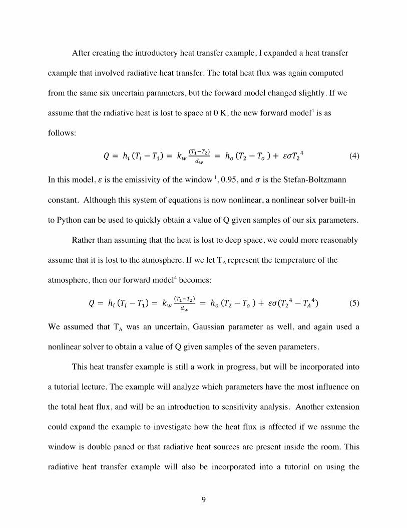
After creating the introductory heat transfer example, I expanded a heat transfer

example that involved radiative heat transfer. The total heat flux was again computed

from the same six uncertain parameters, but the forward model changed slightly. If we

assume that the radiative heat is lost to space at 0 K, the new forward model4 is as

follows:

𝑄 =  ℎ!   𝑇! − 𝑇! =  𝑘!(!!!!!)!!

 =  ℎ!   𝑇! − 𝑇!   +  𝜀𝜎𝑇!! (4)

In this model, 𝜀 is the emissivity of the window 1, 0.95, and 𝜎 is the Stefan-Boltzmann

constant. Although this system of equations is now nonlinear, a nonlinear solver built-in

to Python can be used to quickly obtain a value of Q given samples of our six parameters.

Rather than assuming that the heat is lost to deep space, we could more reasonably

assume that it is lost to the atmosphere. If we let TA represent the temperature of the

atmosphere, then our forward model4 becomes:

𝑄 =  ℎ!   𝑇! − 𝑇! =  𝑘!!!!!!!!

 =  ℎ!   𝑇! − 𝑇!   +  𝜀𝜎(𝑇!! − 𝑇!!) (5)

We assumed that TA was an uncertain, Gaussian parameter as well, and again used a

nonlinear solver to obtain a value of Q given samples of the seven parameters.

This heat transfer example is still a work in progress, but will be incorporated into

a tutorial lecture. The example will analyze which parameters have the most influence on

the total heat flux, and will be an introduction to sensitivity analysis. Another extension

could expand the example to investigate how the heat flux is affected if we assume the

window is double paned or that radiative heat sources are present inside the room. This

radiative heat transfer example will also be incorporated into a tutorial on using the

 10  

Python interface of UQTk to quantify the uncertainty in output Q through spectral

projection methods. Currently, the examples in the UQTk distribution call C++ apps to

perform these spectral projections, and it is a work in progress to create an example script

that performs this task fully using the Python interface.

V. CONCLUSION

Throughout my SULI internship this summer, I worked on projects to help make

UQ methods more accessible to the scientific community at large. As I was unfamiliar

with these methods myself before I began my internship, I was able to ensure that the

examples I created would be at an appropriate introductory level. As my main task, I

created a tutorial example on using the Python interface of software known as UQTk to

perform numerical integrations. This example consisted of scripts that are included in the

software distribution, along with a thorough explanation of how to use these scripts to run

an example. My second project was to create an example on the fundamentals of UQ to

include in a tutorial lecture that my mentor Bert Debusschere presents at workshops. This

example involved heat transfer through a window, a scenario that is relevant to most

individuals and easy to conceptualize. For my third task, I worked on expanding this heat

transfer example to include radiation. This project is still a work in progress, but will be

incorporated into tutorials lectures in the future.

During my short ten weeks at Sandia, I’ve learned a lot. I got a glimpse into the

field of uncertainty quantification, and saw first hand what unique job opportunities are

available at DOE national laboratories. I gained more experience programming in

 11  

Python, learned how to improve my documentation for files that will be run by others,

and also learned how to write documents in LaTex. These are just a few of the valuable

skills I’ve gained during my SULI internship, and I am very thankful to have had this

learning opportunity.

ACKNOWLEDGMENTS

I’d like to thank my mentor Bert Debusschere for his guidance on my research this

summer, and I’d also like to thank Khachik Sargsyan for his assistance as well. My work

was supported by the U.S. Department of Energy, Office of Science, Office of Advanced

Scientific Computing Research, under Award Number 11-014956. My work was also

supported by the U.S. Department of Energy, Office of Science, Office of Workforce

Development for Teachers and Scientists (WDTS) under the Science Undergraduate

Laboratory Internship (SULI) program. Sandia National Laboratories is a multi-program

laboratory managed and operated by Sandia Corporation, a wholly owned subsidiary of

Lockheed Martin Corporation, for the U.S. Department of Energy’s National Nuclear

Security Administration under contract DE-AC04_94AL85000. SAND

REFERENCES

1Brewster, M. (1992). Thermal radiative transfer and properties. New York: Wiley.

2Debusschere, B. (2015). Polynomial Chaos Based Uncertainty Quantification Lecture 2:

Forward Propagation. Retrieved from http://www.quest-scidac.org/wp-

content/uploads/2015/02/Debusschere_RPI_UQ_Lec2.pdf

 12  

3Debusschere, B. (2015). Polynomial Chaos Based Uncertainty Quantification Lecture 1:

Context and Fundamentals. Retrieved from http://www.quest-scidac.org/wp-

content/uploads/2015/02/Debusschere_RPI_UQ_Lec1.pdf

4Heat Transfer: Radiation. (n.d.). Retrieved August 18, 2015, from

http://www.auburn.edu/academic/classes/matl0501/coursepack/radiation/text.htm

5Sargsyan, K., Safta, C., Chowdhary, K., De Bord, S., & Debusschere, B. (2015). UQTk

Version 3.0 User Manual. 7011 East Ave, Livermore, CA 94550: Sandia National

Laboratories. To be published.

6UQ Toolkit. (n.d.). Retrieved August 18, 2015, from http://www.sandia.gov/uqtoolkit/