Embed Size (px)
Citation preview
©SOFiSTiK AG 2009
Bridge Design
CABD-Concept
SSD Version 2010-5

This manual is protected by copyright laws. No part of it may be translated, copied or
reproduced, in any form or by any means, without written permission from SOFiSTiK AG.
SOFiSTiK reserves the right to modify or to release new editions of this manual.
The manual and the program have been thoroughly checked for errors. However, SOFiSTiK
does not claim that either one is completely error free. Errors and omissions are corrected as
soon as they are detected.
The user of the program is solely responsible for the applications. We strongly encourage the
user to test the correctness of all calculations at least by random sampling.
Bridge Design CABD-Concept
Basics 1
Contents 1 Basics ................................................................................................................................ 3
1.1 Data structure of the SOFiSTiK software ................................................................... 3
1.2 Important SOFiSTiK modules .................................................................................... 4
1.3 Recommended loadcase numbering scheme ............................................................ 5
1.4 Understanding SOFiSTiK ........................................................................................... 6
1.5 Components of the CABD technology ....................................................................... 8
2 Cross Sections .................................................................................................................. 9
2.1 General ...................................................................................................................... 9
2.2 Thick walled cross section ....................................................................................... 10
2.3 Thin walled cross section ......................................................................................... 11
2.4 Using the Cross Section Editor ................................................................................ 13
2.5 Cross section properties and control options ........................................................... 14
2.6 Parametric cross sections ........................................................................................ 16
2.6.1 Point to point ..................................................................................................... 16
2.6.2 Assign variable ................................................................................................. 16
2.6.3 Assign axis ........................................................................................................ 17
2.6.4 Point at line ....................................................................................................... 17
3 Geometry / Defintion of Axes .......................................................................................... 18
4 Structure and Substructure ............................................................................................. 22
5 Tendon Layout ................................................................................................................ 25
6 Classification of actions ................................................................................................... 28
7 Combination rules and Superpositioning ........................................................................ 31
8 Traffic Loading ................................................................................................................ 34
8.1 Moving Load Analysis acc. t. EN 1991-2 ................................................................. 35
8.1.1 Subdivsion into LANES ..................................................................................... 35
8.1.2 Location and numbering of the lanes for design ............................................... 36
8.1.3 Load Model 1 .................................................................................................... 37
8.1.4 Load Model 2 .................................................................................................... 39
8.1.5 Load Model 3 (special vehicles) ....................................................................... 39
8.1.6 Load Model 4 (crowd loading) .......................................................................... 42
8.1.7 Fatique Load Model 1 ....................................................................................... 42
8.1.8 Fatique Load Model 2 ....................................................................................... 42
8.1.9 Fatique Load Model 3 ....................................................................................... 43
8.1.10 Fatique Load Model 4 ....................................................................................... 44
8.1.11 Groups of traffic loads ....................................................................................... 45
Bridge Design CABD-Concept
Basics 2
8.2 Load stepping method ............................................................................................. 46
8.3 Influence Line Method .............................................................................................. 48
8.4 Highway bridge loading acc. to BS 5400 (BD37/01) ................................................ 51
8.4.1 Subdivision into notional lanes ......................................................................... 51
8.4.2 Definition of loadmodels (HA,HB) ..................................................................... 51
9 Construction stages ........................................................................................................ 52
9.1 Table: Construction Stages ...................................................................................... 52
9.2 Table: Groups .......................................................................................................... 53
9.3 Table: Loads ............................................................................................................ 53
10 Design Code Checks ................................................................................................... 54
Annex A: Examples ................................................................................................................ 55

Bridge Design CABD-Concept
Basics 3
1 Basics This tutorial shall explain the usage of the CABD (Computer Aided Bridge Design) concept
which is available in the 2010 version of the SOFiSTiK FEA software.
All computations are controlled via the SOFiSTiK Structural Desktop SSD; the SSD can be
started using the desktop icon depicted above. Alternatively you can start all programs
directly from the installation directory: e.g. C:\Program Files\SOFiSTiK\2010\ANALYSIS_25
Prerequisites:
The CABD technology requires the CABD license; the influence line evaluation of traffic loads the ELLA license. Please contact your SOFiSTiK reseller or [email protected] in case of vagueness.
Please refer to the basic SSD-SOFiPLUS (Version 2010) tutorial for general information on SSD and SOFiPLUS, the tutorial can be found in the Infoportal: http://www.sofistik.com/infoportal/
The software should be updated using SONAR before starting with this tutorial, the password for update has been send to all SOFiSTiK users having a valid maintenance contract. Please contact [email protected] if you encounter any technical problems.
For installation and SONAR online update information please refer to the Administration manual: SSD Menu ‘Help’ -> ‘SOFiSTiK Documentation…’ ‘administration_1.pdf’
1.1 Data structure of the SOFiSTiK software
• The control data of a computation is stored in a file called [project_name].sofistik.
Geometrical and structural information generated with the AutoCAD based
preprocessor SOFiPLUS(-X) will be in a second file called [project_name].dwg.
These two files are necessary to reproduce the analysis and to generate the CDB.
• All data (elements, results etc.) is stored in the CDB = Central Data Base
[project_name].cdb
• The data written into the CDB can stem from several sources: SOFiPLUS, Revit
Structure, ASCII-Input (CADINP).
• The ANIMATOR shows animated geometric and result information from the CDB.
• The SSD – SOFiSTiK Structural Desktop – controls all modules and allows running
the calculation.
Bridge Design CABD-Concept
Basics 4
• Should data be prepared in ASCII-Input only, TEDDY is the alternative to the SSD.
File name: [project_name].dat.
• Further information can be found in the basic manual: SSD Menu ‘Help’ -> ‘SOFiSTiK
Documentation…’ ‘sofistik_1.pdf’
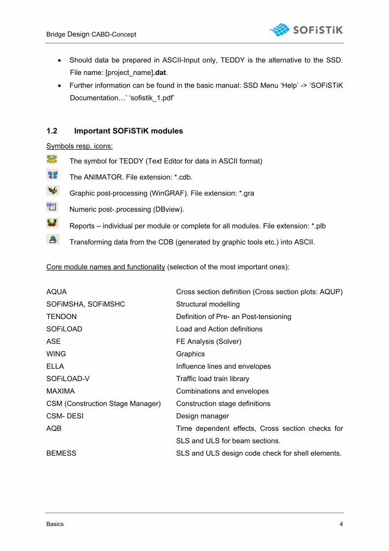
1.2 Important SOFiSTiK modules
Symbols resp. icons:
The symbol for TEDDY (Text Editor for data in ASCII format)
The ANIMATOR. File extension: *.cdb.
Graphic post-processing (WinGRAF). File extension: *.gra
Numeric post-.processing (DBview).
Reports – individual per module or complete for all modules. File extension: *.plb
Transforming data from the CDB (generated by graphic tools etc.) into ASCII.
Core module names and functionality (selection of the most important ones):
AQUA Cross section definition (Cross section plots: AQUP)
SOFiMSHA, SOFiMSHC Structural modelling
TENDON Definition of Pre- an Post-tensioning
SOFiLOAD Load and Action definitions
ASE FE Analysis (Solver)
WING Graphics
ELLA Influence lines and envelopes
SOFiLOAD-V Traffic load train library
MAXIMA Combinations and envelopes
CSM (Construction Stage Manager) Construction stage definitions
CSM- DESI Design manager
AQB Time dependent effects, Cross section checks for
SLS and ULS for beam sections.
BEMESS SLS and ULS design code check for shell elements.
Bridge Design CABD-Concept
Basics 5
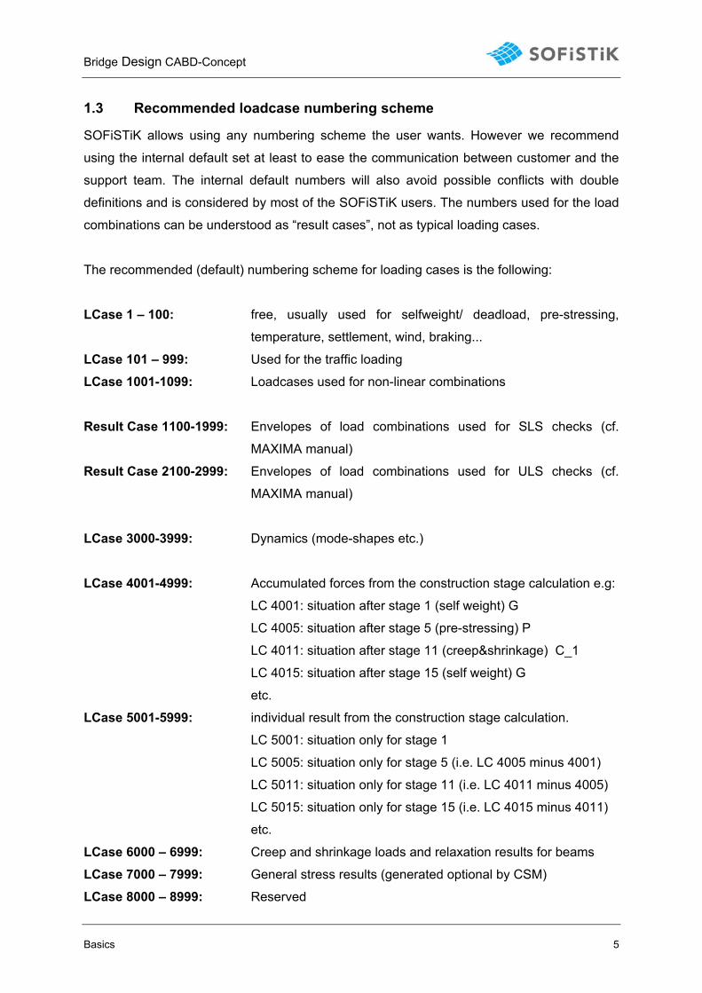
1.3 Recommended loadcase numbering scheme
SOFiSTiK allows using any numbering scheme the user wants. However we recommend
using the internal default set at least to ease the communication between customer and the
support team. The internal default numbers will also avoid possible conflicts with double
definitions and is considered by most of the SOFiSTiK users. The numbers used for the load
combinations can be understood as “result cases”, not as typical loading cases.
The recommended (default) numbering scheme for loading cases is the following:
LCase 1 – 100: free, usually used for selfweight/ deadload, pre-stressing,
temperature, settlement, wind, braking...
LCase 101 – 999: Used for the traffic loading
LCase 1001-1099: Loadcases used for non-linear combinations
Result Case 1100-1999: Envelopes of load combinations used for SLS checks (cf.
MAXIMA manual)
Result Case 2100-2999: Envelopes of load combinations used for ULS checks (cf.
MAXIMA manual)
LCase 3000-3999: Dynamics (mode-shapes etc.)
LCase 4001-4999: Accumulated forces from the construction stage calculation e.g:
LC 4001: situation after stage 1 (self weight) G
LC 4005: situation after stage 5 (pre-stressing) P
LC 4011: situation after stage 11 (creep&shrinkage) C_1
LC 4015: situation after stage 15 (self weight) G
etc.
LCase 5001-5999: individual result from the construction stage calculation.
LC 5001: situation only for stage 1
LC 5005: situation only for stage 5 (i.e. LC 4005 minus 4001)
LC 5011: situation only for stage 11 (i.e. LC 4011 minus 4005)
LC 5015: situation only for stage 15 (i.e. LC 4015 minus 4011)
etc.
LCase 6000 – 6999: Creep and shrinkage loads and relaxation results for beams
LCase 7000 – 7999: General stress results (generated optional by CSM)
LCase 8000 – 8999: Reserved
Bridge Design CABD-Concept
Basics 6
9001 – 9999: Eigenmodes for response spectra analysis
1.4 Understanding SOFiSTiK
General workflow sequence in SOFiSTiK is as follows:
1. Model creation and load definition: a. Code
b. Materials
c. Cross Sections
d. Geometry of the structure
e. Tendon Layout, Prestressing
f. Basic loads
g. Moving Loads (traffic)
2. Loadcase analysis (characteristic loads) and/or Influence line evaluation 3. Intermediate Superpositioning (all variable actions/ loadcases) of inner forces
related to the total cross section (final stage). 4. Final-Superpositioning (Dead load, superimposed dead load, prestress,
creep&shrinkage&relaxation, envelopes of variable loads) of inner forces related to
the partial cross sections.
5. Design Code Checks a. ULS Design for required reinforcement, bearing capacity calculation and other
ultimate cases.
b. SLS Design: Serviceability checks (fibre stress checks, crack width check,
displacements of the structure, fatigue, dynamics etc.)
Bridge Design CABD-Concept
Basics 7
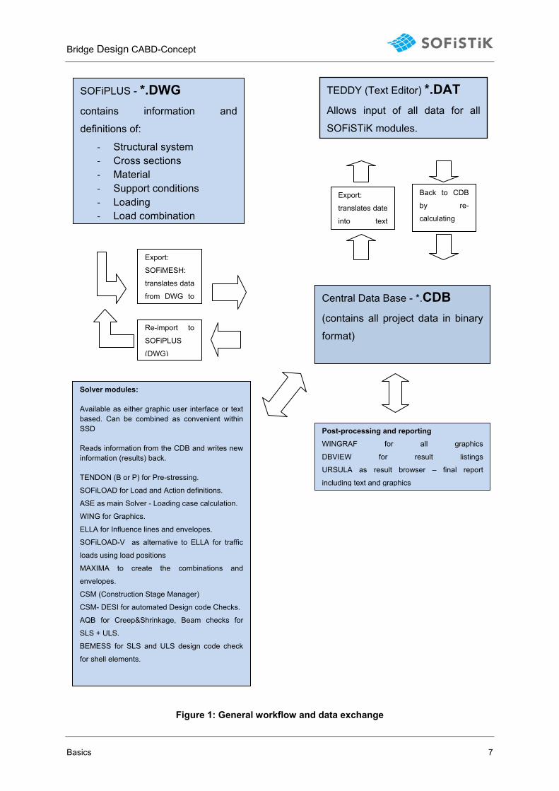
Figure 1: General workflow and data exchange
Central Data Base - *.CDB
(contains all project data in binary
format)
SOFiPLUS - *.DWG
contains information and
definitions of:
‐ Structural system ‐ Cross sections ‐ Material ‐ Support conditions ‐ Loading ‐ Load combination
Export:
SOFiMESH:
translates data
from DWG to
TEDDY (Text Editor) *.DAT
Allows input of all data for all
SOFiSTiK modules.
Export:
translates date
into text
Back to CDB
by re-
calculating
Re-import to
SOFiPLUS
(DWG)
Post-processing and reporting WINGRAF for all graphics
DBVIEW for result listings
URSULA as result browser – final report
including text and graphics
Solver modules:
Available as either graphic user interface or text based. Can be combined as convenient within SSD
Reads information from the CDB and writes new information (results) back.
TENDON (B or P) for Pre-stressing.
SOFiLOAD for Load and Action definitions.
ASE as main Solver - Loading case calculation.
WING for Graphics.
ELLA for Influence lines and envelopes.
SOFiLOAD-V as alternative to ELLA for traffic
loads using load positions
MAXIMA to create the combinations and
envelopes.
CSM (Construction Stage Manager)
CSM- DESI for automated Design code Checks.
AQB for Creep&Shrinkage, Beam checks for
SLS + ULS.
BEMESS for SLS and ULS design code check
for shell elements.
Bridge Design CABD-Concept
Basics 8
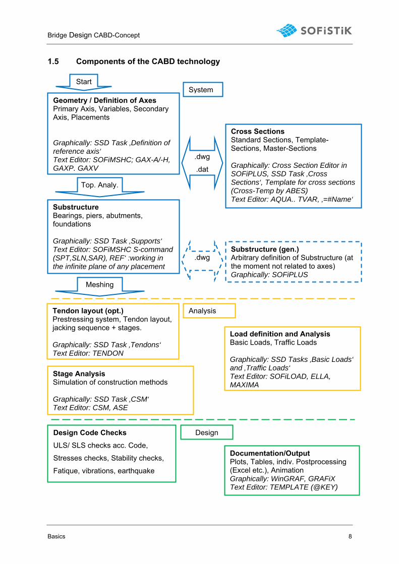
1.5 Components of the CABD technology
Geometry / Definition of Axes Primary Axis, Variables, Secondary Axis, Placements Graphically: SSD Task ‚Definition of reference axis‘ Text Editor: SOFiMSHC; GAX-A/-H, GAXP, GAXV
Cross Sections Standard Sections, Template-Sections, Master-Sections Graphically: Cross Section Editor in SOFiPLUS, SSD Task ‚Cross Sections‘, Template for cross sections (Cross-Temp by ABES) Text Editor: AQUA.. TVAR, ‚=#Name‘
.dwg
.dat
Top. Analy.
Substructure Bearings, piers, abutments, foundations Graphically: SSD Task ‚Supports‘ Text Editor: SOFiMSHC S-command (SPT,SLN,SAR)‚ REF‘ :working in the infinite plane of any placement
.dwg Substructure (gen.) Arbitrary definition of Substructure (at the moment not related to axes) Graphically: SOFiPLUS
Meshing
Load definition and Analysis Basic Loads, Traffic Loads Graphically: SSD Tasks ‚Basic Loads‘ and ‚Traffic Loads‘ Text Editor: SOFiLOAD, ELLA, MAXIMA
Start System
Analysis
Design
Stage Analysis Simulation of construction methods Graphically: SSD Task ‚CSM‘ Text Editor: CSM, ASE
Design Code Checks ULS/ SLS checks acc. Code,
Stresses checks, Stability checks,
Fatique, vibrations, earthquake
Documentation/Output Plots, Tables, indiv. Postprocessing (Excel etc.), Animation Graphically: WinGRAF, GRAFiX Text Editor: TEMPLATE (@KEY)
Tendon layout (opt.) Prestressing system, Tendon layout, jacking sequence + stages. Graphically: SSD Task ‚Tendons‘ Text Editor: TENDON
Bridge Design CABD-Concept
Cross Sections 9
2 Cross Sections There are three types of cross sections in SOFiSTiK, depending on the complexity of the
design task we differ between:
• Standard Sections
• Thick walled sections (recommended for: polygonal cross sections e.g. R/C sections)
• Thin walled sections (recommended for: slender cross sections, welded sections,
composite steel-concrete sections)
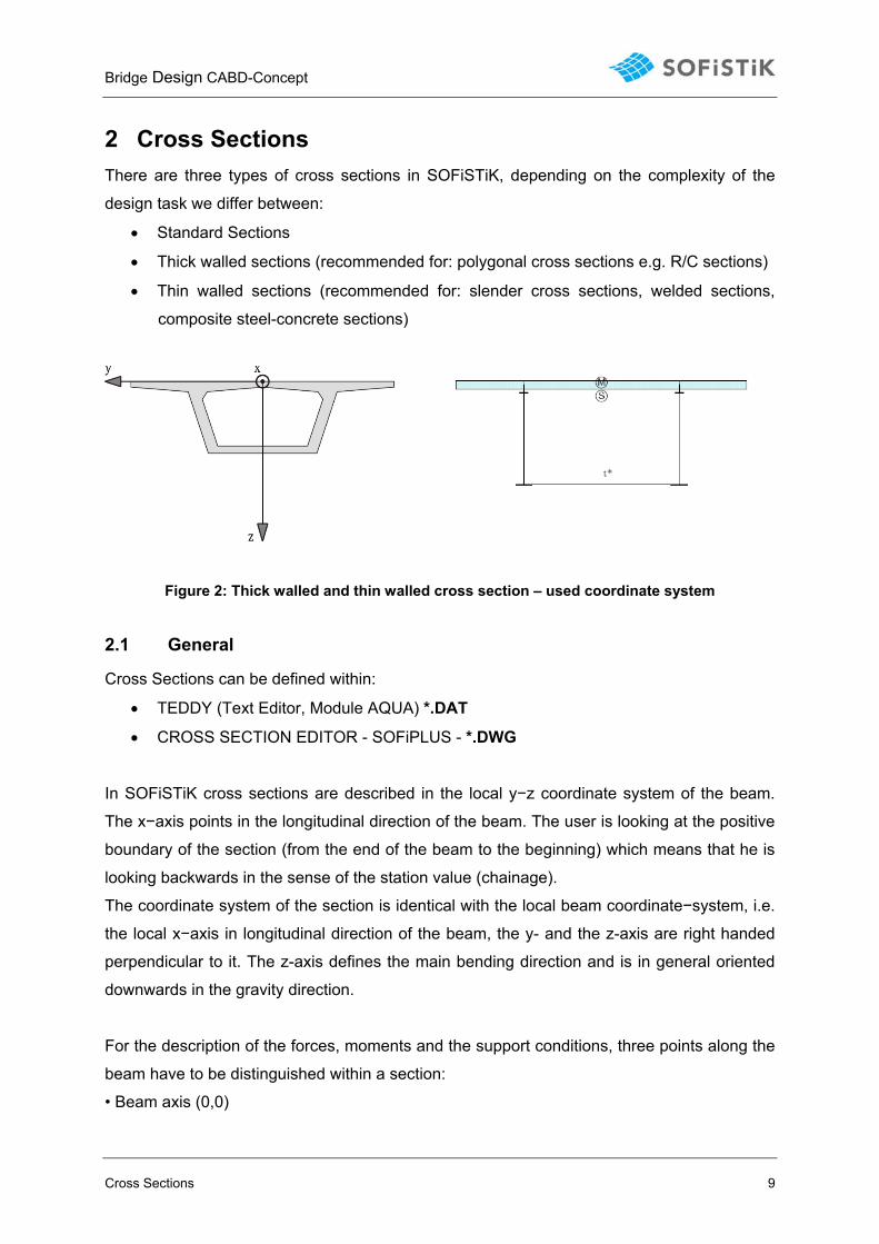
Figure 2: Thick walled and thin walled cross section – used coordinate system
2.1 General
Cross Sections can be defined within:
• TEDDY (Text Editor, Module AQUA) *.DAT
• CROSS SECTION EDITOR - SOFiPLUS - *.DWG
In SOFiSTiK cross sections are described in the local y−z coordinate system of the beam.
The x−axis points in the longitudinal direction of the beam. The user is looking at the positive
boundary of the section (from the end of the beam to the beginning) which means that he is
looking backwards in the sense of the station value (chainage).
The coordinate system of the section is identical with the local beam coordinate−system, i.e.
the local x−axis in longitudinal direction of the beam, the y- and the z-axis are right handed
perpendicular to it. The z-axis defines the main bending direction and is in general oriented
downwards in the gravity direction.
For the description of the forces, moments and the support conditions, three points along the
beam have to be distinguished within a section:
• Beam axis (0,0)
Bridge Design CABD-Concept
Cross Sections 10
This point may be given either by the center of gravity of the sections (centric beam) or it is
defined by the origin of the sectional coordinate system (beam with a reference axis).
Support conditions in the nodes thus are always specified relative to the beam axis position!
• Center of gravity (S)
This point is the reference for the normal force and the bending moments
• Shear center (M)
This point is the reference for the transverse shear force and the torsional moment. The
section will rotate about that point in general.
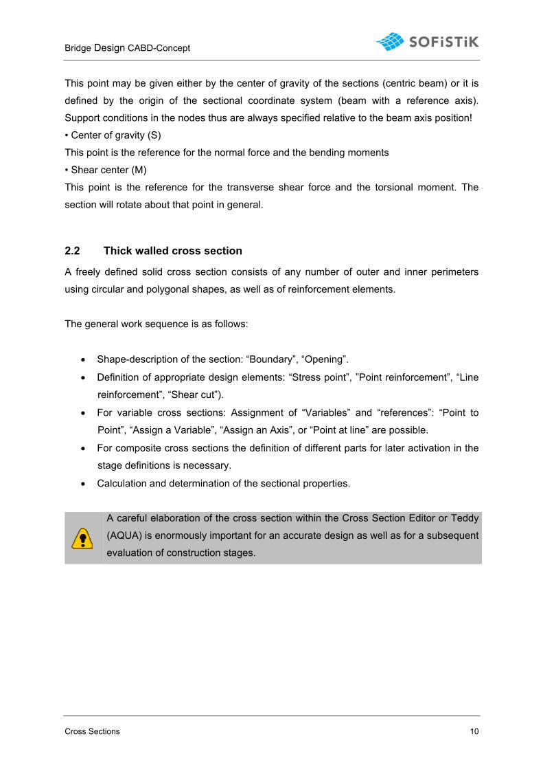
2.2 Thick walled cross section
A freely defined solid cross section consists of any number of outer and inner perimeters
using circular and polygonal shapes, as well as of reinforcement elements.
The general work sequence is as follows:
• Shape-description of the section: “Boundary”, “Opening”.
• Definition of appropriate design elements: “Stress point”, ”Point reinforcement”, “Line
reinforcement”, “Shear cut”).
• For variable cross sections: Assignment of “Variables” and “references”: “Point to
Point”, “Assign a Variable”, “Assign an Axis”, or “Point at line” are possible.
• For composite cross sections the definition of different parts for later activation in the
stage definitions is necessary.
• Calculation and determination of the sectional properties.
A careful elaboration of the cross section within the Cross Section Editor or Teddy
(AQUA) is enormously important for an accurate design as well as for a subsequent
evaluation of construction stages.
Bridge Design CABD-Concept
Cross Sections 11
Figure 3: Cross Section Editor - Thick walled elements
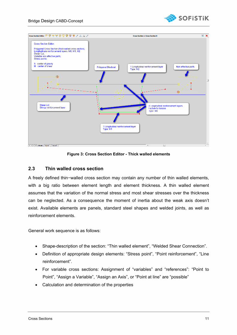
2.3 Thin walled cross section
A freely defined thin−walled cross section may contain any number of thin walled elements,
with a big ratio between element length and element thickness. A thin walled element
assumes that the variation of the normal stress and most shear stresses over the thickness
can be neglected. As a consequence the moment of inertia about the weak axis doesn’t
exist. Available elements are panels, standard steel shapes and welded joints, as well as
reinforcement elements.
General work sequence is as follows:
• Shape-description of the section: “Thin walled element”, “Welded Shear Connection”.
• Definition of appropriate design elements: “Stress point”, “Point reinforcement”, “Line
reinforcement”.
• For variable cross sections: Assignment of “variables” and “references”: “Point to
Point”, “Assign a Variable”, “Assign an Axis”, or “Point at line” are “possible”
• Calculation and determination of the properties
Bridge Design CABD-Concept
Cross Sections 12
Figure 4: Cross Section Editor - Thin walled elements
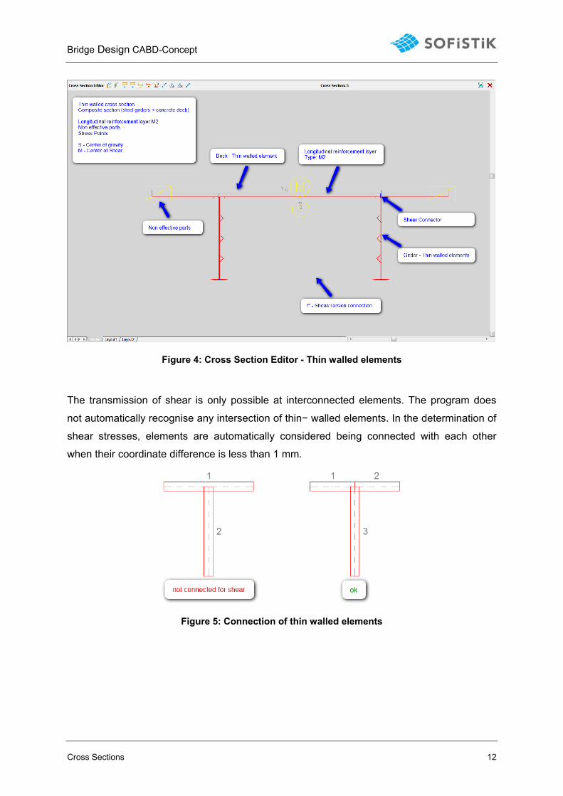
The transmission of shear is only possible at interconnected elements. The program does
not automatically recognise any intersection of thin− walled elements. In the determination of
shear stresses, elements are automatically considered being connected with each other
when their coordinate difference is less than 1 mm.
Figure 5: Connection of thin walled elements
Bridge Design CABD-Concept
Cross Sections 13
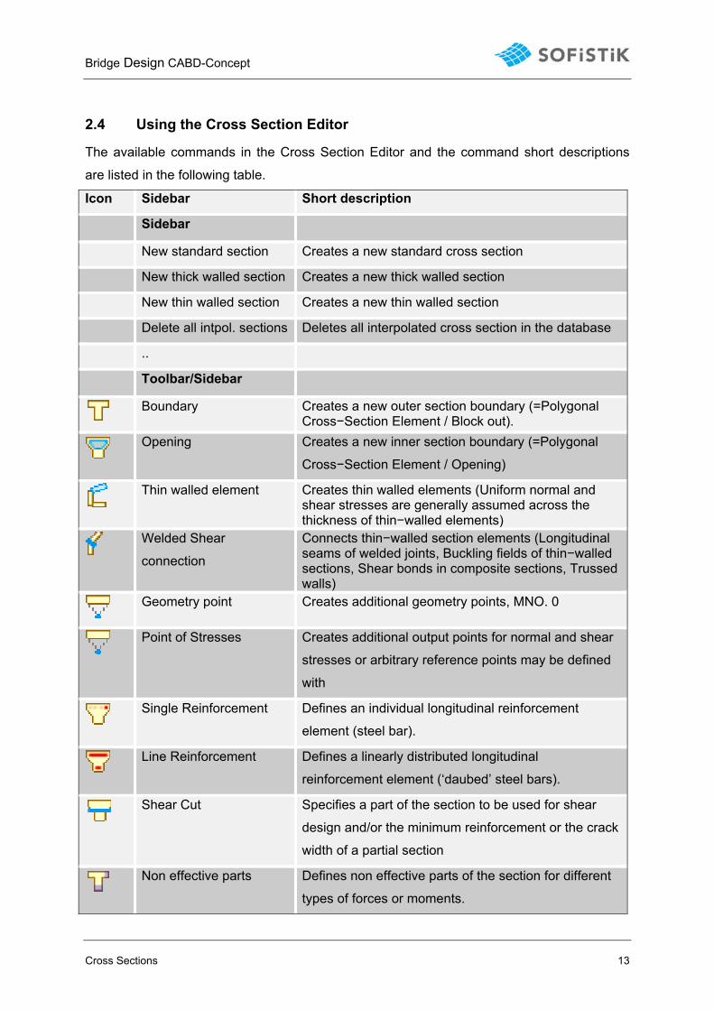
2.4 Using the Cross Section Editor
The available commands in the Cross Section Editor and the command short descriptions
are listed in the following table.
Icon Sidebar Short description
Sidebar New standard section Creates a new standard cross section
New thick walled section Creates a new thick walled section
New thin walled section Creates a new thin walled section
Delete all intpol. sections Deletes all interpolated cross section in the database
..
Toolbar/Sidebar
Boundary Creates a new outer section boundary (=Polygonal
Cross−Section Element / Block out).
Opening Creates a new inner section boundary (=Polygonal
Cross−Section Element / Opening)
Thin walled element Creates thin walled elements (Uniform normal and
shear stresses are generally assumed across the thickness of thin−walled elements)
Welded Shear
connection
Connects thin−walled section elements (Longitudinal seams of welded joints, Buckling fields of thin−walled sections, Shear bonds in composite sections, Trussed walls)
Geometry point Creates additional geometry points, MNO. 0
Point of Stresses Creates additional output points for normal and shear
stresses or arbitrary reference points may be defined
with
Single Reinforcement Defines an individual longitudinal reinforcement
element (steel bar).
Line Reinforcement Defines a linearly distributed longitudinal
reinforcement element (‘daubed’ steel bars).
Shear Cut Specifies a part of the section to be used for shear
design and/or the minimum reinforcement or the crack
width of a partial section
Non effective parts Defines non effective parts of the section for different
types of forces or moments.
Bridge Design CABD-Concept
Cross Sections 14
rolled steel shapes Insert rolled steel shapes, e.g. to define compound
sections (thick or thinwalled)
Point to point Creates a constant reference between 2 vertexes (y-
coordinate, z- coordinate, both the y- and z-
coordinate).
Assign variable Assigns a predefined variable progress to vertices (y-
coordinate, z- coordinate, both the y- and z-
coordinate).
Assign axis Assigns a predefined axis to vertices
(y- coordinate, z- coordinate, both the y- and z-
coordinate).
Point at line Creates a reference point, following up to two other
points within the cross section, this point may then a
variable be assigned e.g.: variable height of inclined
webs
2.5 Cross section properties and control options
Properties and control options of any cross section may be defined and modified in the
general properties dialogue.
Properties: In the Tab ‚properties‘, number, name and material of the cross section may be
specified.
The reference material number should, in general, be specified in this tab. The declaration of
a material number with individual cross section elements is only appropriate for composite
cross sections. In case of composite sections, ideal cross section values are calculated
based on the material defined in the Tab properties:
Eref... Young-Modulus of the material specified in the Tab ‘Properties’
Ei… Young-Modulus of the material used for the cross section elements
Ai… Area of the cross section element
Control values: Parameters for the analysis of the cross section might be specified in this tab.
Depending on the type of cross section, different methods of cross section analysis will take
Bridge Design CABD-Concept
Cross Sections 15
place. Note: only for experienced users (for more information we refer to the manual of
module AQUA).
Additional values: The tab might be used for input of additional cross section values, such as
reduced torsion stiffness values, buckling strain curves, effective thickness, etc.
Layers: The user may specify up to ten longitudinal reinforcement layers with different types
for each cross section. There are layers with the minimum reinforcement (M0 − M9) and
extra layers (Z0−Z9).
• M−Layers have minimum reinforcement and, in the absence of any other instructions,
they are laid by at least the specified AS values when doing a design.
• On the other hand, Z−Layers may be not activated at all. The layer number has no
influence on the selection of a particular layer by the reinf. design module.
For ideal sectional values only the minimum values of the reinforcements will be used.
If, however, processing in the order of the layer numbers is desired, the layer numbers S0 −
S9 should be used as a special case.
• S−Layers cannot be used in combination with M− or Z−layers. As an exception to this
rule, a minimum reinforcement can be defined for the lowest layer by M0.
The ratios of the layers to each other are controlled by the layer type.
Variables: Variables assigned to vertexes and elements of the cross section are listed in this
table.
Construction stages within the section: The user may specify up to 9 construction stages for
each cross section. The construction stages are assigned to the individual elements of the
section. The section is subdivided in as many parts as there are stages for composing the
total section.
If a part of the section is active only temporarily, a CS “No.” for the “Expiry” of this part may
be specified. This is then the last construction stage where this cross section part is active.
The individual parts and sectional values of the section with number “No.” may be addressed
via a sub−number as:
Part No. is the complete section
Part No.1 is the first construction stage (even though if the first construction stage number
isn’t 1)
Part No.2 is the second construction stage
Etc.
Bridge Design CABD-Concept
Cross Sections 16
2.6 Parametric cross sections
It is very common, especially in the bridge design, that very similar sections are derived from
a template (master cross section). The Cross Section Editor and module AQUA will therefore
not only allow this parametric approach, but it will also store the parametric information of the
cross section in the database CDB, in order to allow easy prototyping.
Primary solution for that task are formula expressions to be defined for any coordinate with
up to 256 characters in the form of “=formula”. These formulas are stored together with the
section and may be reevaluated for any section with different values along an axis or with
explicit definitions locally.
The Cross Section Editor offers the following commands:
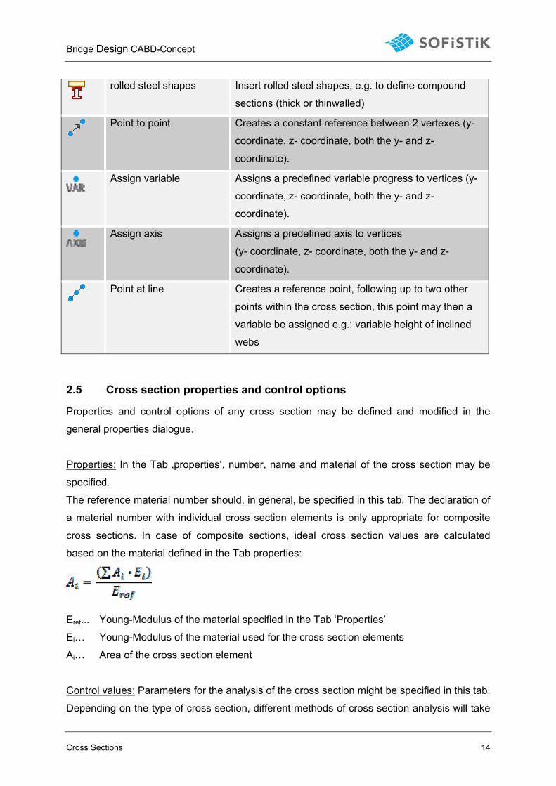
2.6.1 Point to point
The command creates a constant link between 2 coordinates (y- coordinate, z- coordinate,
and both the y- and z-coordinate).
Figure 6: Point to point (Rechtswert/Hochwert = Right/Up-Value)
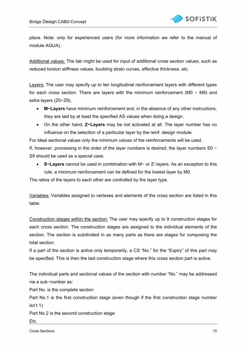
2.6.2 Assign variable
Assigns a formula expression to any coordinate (vertex or element: y- coordinate, z-
coordinate, both the y- and z-coordinate).
Figure 7: Assign variable (Rechtswert/Hochwert = Right/Up-Value)
Bridge Design CABD-Concept
Cross Sections 17
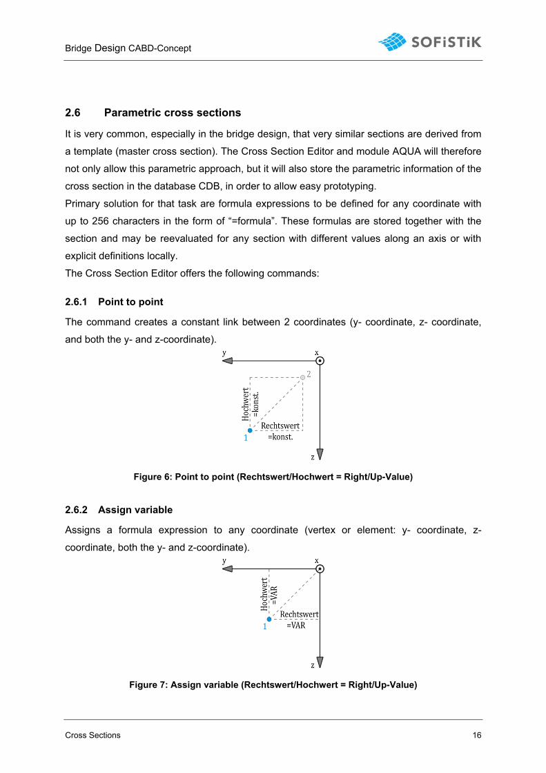
2.6.3 Assign axis
Assigns the progress of a freely defined axis to any coordinate (vertex or element: y-
coordinate, z- coordinate, both the y- and z-coordinate).
Figure 8: Assign axis (Rechtswert/Hochwert = Right/Up-Value)
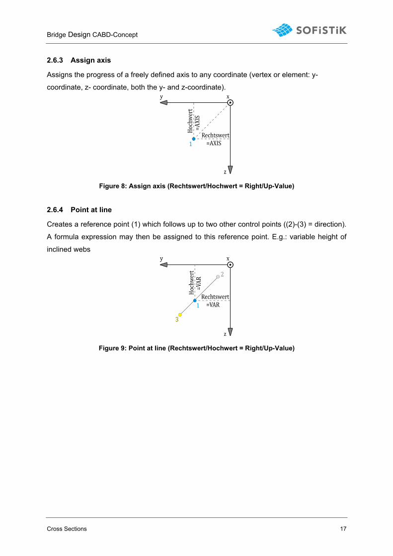
2.6.4 Point at line
Creates a reference point (1) which follows up to two other control points ((2)-(3) = direction).
A formula expression may then be assigned to this reference point. E.g.: variable height of
inclined webs
Figure 9: Point at line (Rechtswert/Hochwert = Right/Up-Value)
Bridge Design CABD-Concept
Geometry / Defintion of Axes 18
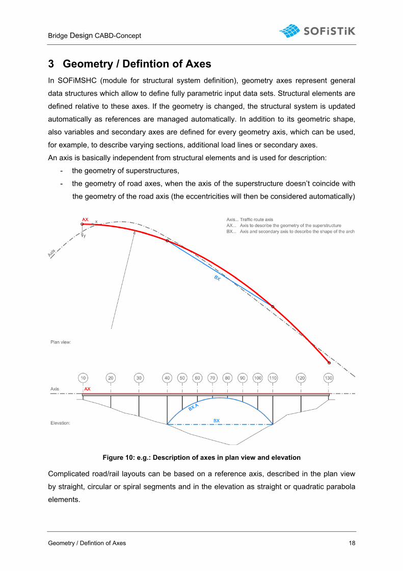
3 Geometry / Defintion of Axes In SOFiMSHC (module for structural system definition), geometry axes represent general
data structures which allow to define fully parametric input data sets. Structural elements are
defined relative to these axes. If the geometry is changed, the structural system is updated
automatically as references are managed automatically. In addition to its geometric shape,
also variables and secondary axes are defined for every geometry axis, which can be used,
for example, to describe varying sections, additional load lines or secondary axes.
An axis is basically independent from structural elements and is used for description:
- the geometry of superstructures,
- the geometry of road axes, when the axis of the superstructure doesn’t coincide with
the geometry of the road axis (the eccentricities will then be considered automatically)
Figure 10: e.g.: Description of axes in plan view and elevation
Complicated road/rail layouts can be based on a reference axis, described in the plan view
by straight, circular or spiral segments and in the elevation as straight or quadratic parabola
elements.
Bridge Design CABD-Concept
Geometry / Defintion of Axes 19
The following commands are available in SOFiMSHC:
GAX Definition of axes
*GAXA / GAXH Alignment axes in plan view / and elevation
*GAXB Straight lines and circular arcs in 3D
*GAXS Secondary axes
*GAXP Placements: special positions along an axis
*GAXV Definition of variables along an axis
*command requires a valid CABD licence
An axis starts with a start point (station at start + coordinate) and a tangential direction,
followed by any number of single alignment elements (straight, circular or spiral segments).
The elevation (GAXH) of the alignment axis is defined at specific stations “S” along the axis
with the corresponding height above datum value.
Using the command GAXB straight or circular axes may be defined by coordinates
(and not by starting coordinates and a tangential direction), so that the definition of
vertical axes becomes possible as well.
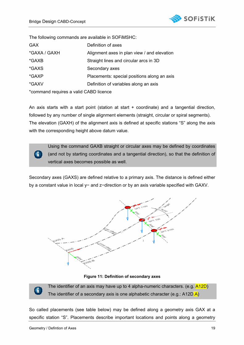
Secondary axes (GAXS) are defined relative to a primary axis. The distance is defined either
by a constant value in local y− and z−direction or by an axis variable specified with GAXV.
Figure 11: Definition of secondary axes
The identifier of an axis may have up to 4 alpha-numeric characters. (e.g. A12D)
The identifier of a secondary axis is one alphabetic character (e.g.: A12D.A)
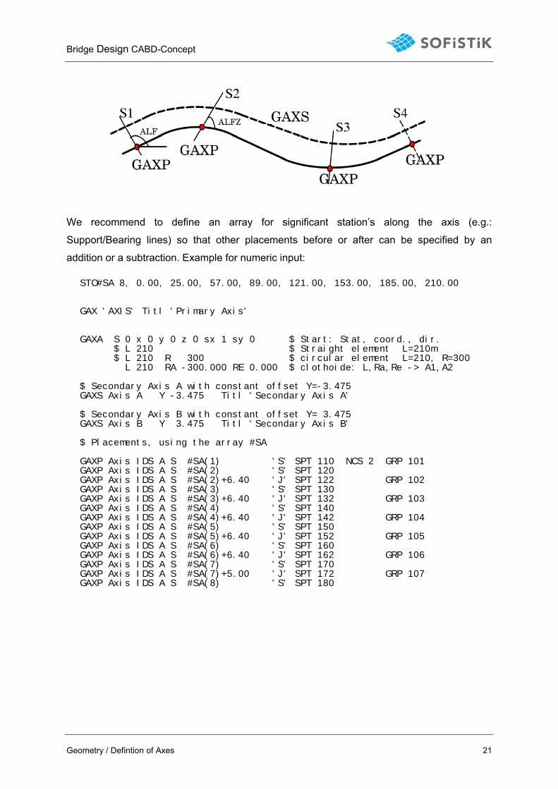
So called placements (see table below) may be defined along a geometry axis GAX at a
specific station “S”. Placements describe important locations and points along a geometry
Bridge Design CABD-Concept
Geometry / Defintion of Axes 20
axis. Wherever structural changes and dependencies will take place a placement has to be
introduced, by means of defining their geometric location and structural boundary conditions
along the axis.
Geometric information Structural information
Pla
cem
ent
- Station value along the axis
- Rotation about the global Z direction
- Skew about the local x−axis
- Skew about transverse y−axis
- Skew about vertical z−axis
- Cross fall to the right (+y)
- Cross fall to the left (−y) see sign
convention in 2.1
- Number of structural point to be
created at the placement.
- Group number of the following
elements.
- Cross−section number of the
subsequent elements or number
before and after the placement given
as Literal ’ncs1:ncs2’.
For each placement a structural point is created on the axis. The node number of this
structural point is set at SPT. Structural lines from point to point are created, which get the
number of their preceding point assigned. The user may specify a group or section number
for a specific placement on the axis which is then used for all subsequent beam elements
created unless one of the numbers is changed. The generation of the structural elements
basically starts at the first placement which has a cross−section number assigned and ends
at the end of the axis or at a placement with type ’E = endface’.
A placement defines an infinite plane at a given station S perpendicular to the axis tangent.
Structural points and other placement properties on secondary axes are created at the
intersection of this plane with the axis.
This infinite plane can be further rotated about the three local axis coordinates by setting
ALFZ, ALFY and ALFX. The infinite plan can also be aligned within the global X−Y
coordinate plane by setting an angle at ALF = {1−360 deg}.
The local coordinate system of the structural point created at the placement is
orientated as default as follows:
local y: perpendicular to the axis at the given station
local x: tangential to the axis at the given station
Bridge Design CABD-Concept
Geometry / Defintion of Axes 21
We recommend to define an array for significant station’s along the axis (e.g.:
Support/Bearing lines) so that other placements before or after can be specified by an
addition or a subtraction. Example for numeric input: STO#SA 8, 0.00, 25.00, 57.00, 89.00, 121.00, 153.00, 185.00, 210.00 GAX 'AXIS' Titl 'Primary Axis' GAXA S 0 x 0 y 0 z 0 sx 1 sy 0 $ Start: Stat, coord., dir. $ L 210 $ Straight element L=210m $ L 210 R 300 $ circular element L=210, R=300 L 210 RA -300.000 RE 0.000 $ clothoide: L,Ra,Re -> A1,A2 $ Secondary Axis A with constant offset Y=-3.475 GAXS Axis A Y -3.475 Titl 'Secondary Axis A' $ Secondary Axis B with constant offset Y= 3.475 GAXS Axis B Y 3.475 Titl 'Secondary Axis B' $ Placements, using the array #SA GAXP Axis IDS A S #SA(1) 'S' SPT 110 NCS 2 GRP 101 GAXP Axis IDS A S #SA(2) 'S' SPT 120 GAXP Axis IDS A S #SA(2)+6.40 'J' SPT 122 GRP 102 GAXP Axis IDS A S #SA(3) 'S' SPT 130 GAXP Axis IDS A S #SA(3)+6.40 'J' SPT 132 GRP 103 GAXP Axis IDS A S #SA(4) 'S' SPT 140 GAXP Axis IDS A S #SA(4)+6.40 'J' SPT 142 GRP 104 GAXP Axis IDS A S #SA(5) 'S' SPT 150 GAXP Axis IDS A S #SA(5)+6.40 'J' SPT 152 GRP 105 GAXP Axis IDS A S #SA(6) 'S' SPT 160 GAXP Axis IDS A S #SA(6)+6.40 'J' SPT 162 GRP 106 GAXP Axis IDS A S #SA(7) 'S' SPT 170 GAXP Axis IDS A S #SA(7)+5.00 'J' SPT 172 GRP 107 GAXP Axis IDS A S #SA(8) 'S' SPT 180
Bridge Design CABD-Concept
Structure and Substructure 22
4 Structure and Substructure As already mentioned, we differentiate between “geometry” and “structure”, although each
placement may already contain structural information.
Based on the placement definition, all information is finally converted to structural elements
(structural points, structural lines) when meshing. The meshing creates the final finite
elements. For meshing we can use:
CTRL MESH to define the bit pattern for mesh generation (beam or shell systems).
CTRL TOPO to enforce a topological analysis.
CTRL HMIN to specify the maximum element size.
CTRL NODE to set up the automatic node numbering.
Module SOFiMSHC allows working in the infinite plane of any placement defined on the
geometry axis. Coordinates of a structural point can be defined relative to a placement. The
coordinates can be given in Euclidian coordinates x, y, z relative to the reference point and
its direction.
This becomes important when parts of the substructure should be defined relative to the
placement or oriented towards to it. In this way these structural elements are updated
automatically if the geometry of the axis is changed.
We recommend making use of the input facilities in relative coordinates, related to a
placement located on an axis.
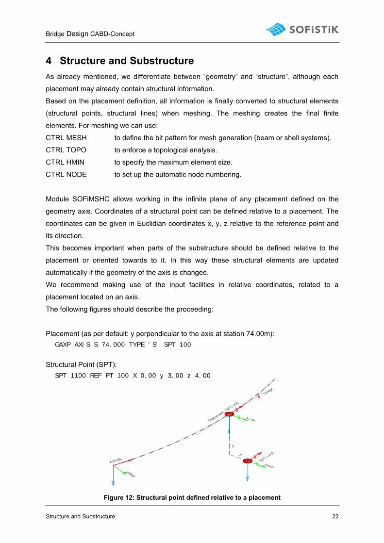
The following figures should describe the proceeding:
Placement (as per default: y perpendicular to the axis at station 74.00m): GAXP AXiS S 74.000 TYPE 'S' SPT 100
Structural Point (SPT): SPT 1100 REF PT 100 X 0.00 y 3.00 z 4.00
Figure 12: Structural point defined relative to a placement
Bridge Design CABD-Concept
Structure and Substructure 23
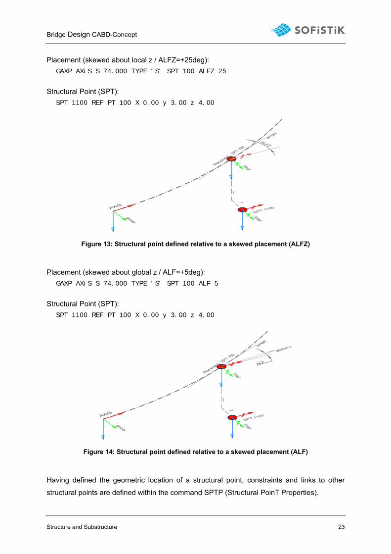
Placement (skewed about local z / ALFZ=+25deg): GAXP AXiS S 74.000 TYPE 'S' SPT 100 ALFZ 25
Structural Point (SPT): SPT 1100 REF PT 100 X 0.00 y 3.00 z 4.00
Figure 13: Structural point defined relative to a skewed placement (ALFZ)
Placement (skewed about global z / ALF=+5deg): GAXP AXiS S 74.000 TYPE 'S' SPT 100 ALF 5
Structural Point (SPT): SPT 1100 REF PT 100 X 0.00 y 3.00 z 4.00
Figure 14: Structural point defined relative to a skewed placement (ALF)
Having defined the geometric location of a structural point, constraints and links to other
structural points are defined within the command SPTP (Structural PoinT Properties).
Bridge Design CABD-Concept
Structure and Substructure 24
Exemplary input (Structural point, Rigid link, Elastic link, Structural line): SPT 1101 REF PT 100 X 0 Y 2.75 Z 3.5 ; SPTP KF ref 100 grp 10 SPTP CX ref 1103 val 1.0 grp 10 SPTP CY ref 1103 val 1.0e7 grp 10 SPTP CZ ref 1103 val 1.0e7 grp 10 SPT 1102 REF PT 100 X 0 Y 2.75 Z 3.5 ; SPTP KF ref 100 grp 10 SPTP CX ref 1104 val 1.0 grp 10 SPTP NCY ref 1104 val 1.0 grp 10 SPTP CZ ref 1104 val 1.0e7 grp 10 SPT 1103 REF PT 100 X 0 Y 2.75 Z 3.5 ; SPTP KF ref 1105 grp 10 SPT 1104 REF PT 100 X 0 Y 2.75 Z 3.5 ; SPTP KF ref 1105 grp 10 SPT 1105 REF PT 100 X 0 Y 0.00 Z 3.5 fix F sLN 1 NPA 1 2 SNO 1 KR DXLN 'Axis' 100.0 The structural point no. 100 is a placement defined on the axis. All structural points (1101,
1102, 1103, 1104) are then defined relatively to it. Support conditions, rigid links or elastic
links may be described as property of a structural point (SPTP) respectively two SPT’s.
Geometric axes may also be used as reference for inner and/or outer boundaries of
structural areas; so that the shape of shell elements can be described with geometric axes
as well.
Exemplary input (Structural area): sln 1 710 610 sln 2 610 620 ref 'Axis.A' $Boundary secondary axis Axis.A sln 3 620 720 sln 4 720 710 ref 'Axis.B' $Boundary secondary axis Axis.B $ Structural area (SAR) with boundary sarb nl 1,2,3,4 (=Structural lines) sar 1 mno 22 mrf 11 nra 7 t .32 Qref belo grp 51 h1 1.00 titl ‘slab’ sarb nl 1,2,3,4 The structural points (610,710,620,720) used for the defintion of structural lines (1,2,3,4) are
placements on the secondary axes (Axis.A and Axis.B).
Bridge Design CABD-Concept
Tendon Layout 25
5 Tendon Layout In SOFiSTiK the prestressing is defined only if a valid structural system is stored in the
database.
The general work sequence for defining prestressung in Module “Tendon” is as follows:
- Prestressing system with material definitions in addition to the already existing
prestressing material.
- Reference Axis and automatic search of a continuous beam series (no gaps)
- Duct and tendon geometry
- Tendon assignment to (construction stages, jacking sequence, friction loss, etc.)
- Calculation of losses (friction and wobble).
- Storage of prestressing as loading case (Primary and secondary effects).
Prestressing system:
First of all an appropriate prestressing system has to be defined (SSD-Task: Prestressing
System). The prestressing system will be stored with a number (keyword NOPS) in the
database and is selected within TENDON.
Reference Axis: a so called reference axis is the base of any tendon definition.
We recommend to either refer directly to a geometry axis (defined within SOFiMSHC), AXES NOH 1 TYPE REFB Axis
... or to make use of the automatic beam search between start and end nodes. AXES NOH 1 TYPE REFB Auto 10 210
In both cases TENDON will search for continuous beam series along this reference axis
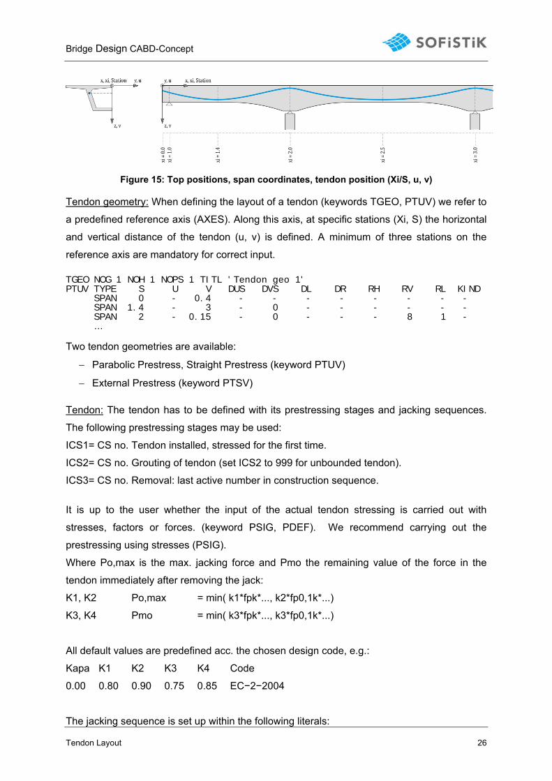
(AXES), to which the tendons finally belong. Top positions (keyword TOPP) may be defined
along the reference axis, either by nodes or stations. The complete axis will then be divided
into several ‘spans’ so that a definition via span-coordinates (Xi) becomes possible as well. TOPP SP S NOH=1 KIND=REFB $ with S = station on axis in m 0 0 $ start face bridge deck 1 1 $ bearing line 2 38.5 $ bearing line
Bridge Design CABD-Concept
Tendon Layout 26
Figure 15: Top positions, span coordinates, tendon position (Xi/S, u, v)
Tendon geometry: When defining the layout of a tendon (keywords TGEO, PTUV) we refer to
a predefined reference axis (AXES). Along this axis, at specific stations (Xi, S) the horizontal
and vertical distance of the tendon (u, v) is defined. A minimum of three stations on the
reference axis are mandatory for correct input. TGEO NOG 1 NOH 1 NOPS 1 TITL 'Tendon geo 1' PTUV TYPE S U V DUS DVS DL DR RH RV RL KIND SPAN 0 - 0.4 - - - - - - - - SPAN 1.4 - 3 - 0 - - - - - - SPAN 2 - 0.15 - 0 - - - 8 1 - … Two tendon geometries are available:
− Parabolic Prestress, Straight Prestress (keyword PTUV)
− External Prestress (keyword PTSV) Tendon: The tendon has to be defined with its prestressing stages and jacking sequences.
The following prestressing stages may be used:
ICS1= CS no. Tendon installed, stressed for the first time.
ICS2= CS no. Grouting of tendon (set ICS2 to 999 for unbounded tendon).
ICS3= CS no. Removal: last active number in construction sequence.
It is up to the user whether the input of the actual tendon stressing is carried out with
stresses, factors or forces. (keyword PSIG, PDEF). We recommend carrying out the
prestressing using stresses (PSIG).
Where Po,max is the max. jacking force and Pmo the remaining value of the force in the
tendon immediately after removing the jack:
K1, K2 Po,max = min( k1*fpk*..., k2*fp0,1k*...)
K3, K4 Pmo = min( k3*fpk*..., k3*fp0,1k*...)
All default values are predefined acc. the chosen design code, e.g.:
Kapa K1 K2 K3 K4 Code
0.00 0.80 0.90 0.75 0.85 EC−2−2004
The jacking sequence is set up within the following literals:
Bridge Design CABD-Concept
Tendon Layout 27
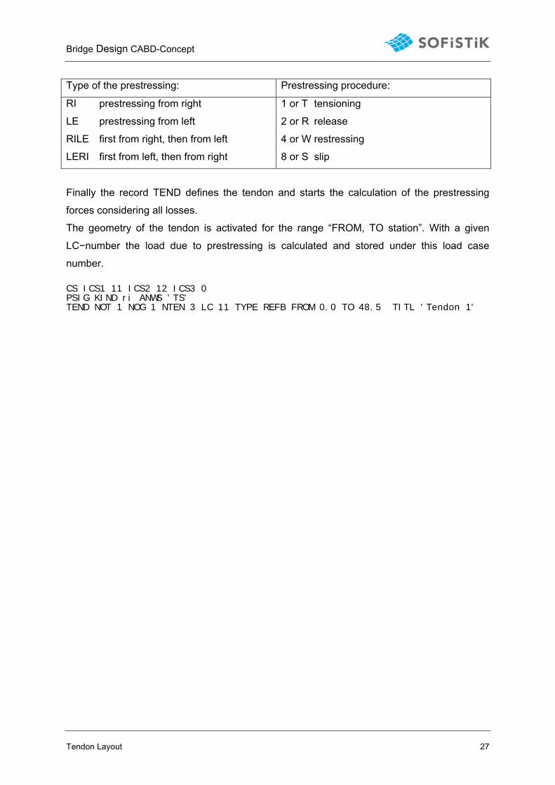
Type of the prestressing: Prestressing procedure:
RI prestressing from right
LE prestressing from left
RILE first from right, then from left
LERI first from left, then from right
1 or T tensioning
2 or R release
4 or W restressing
8 or S slip
Finally the record TEND defines the tendon and starts the calculation of the prestressing
forces considering all losses.
The geometry of the tendon is activated for the range “FROM, TO station”. With a given
LC−number the load due to prestressing is calculated and stored under this load case
number. CS ICS1 11 ICS2 12 ICS3 0 PSIG KIND ri ANWS 'TS' TEND NOT 1 NOG 1 NTEN 3 LC 11 TYPE REFB FROM 0.0 TO 48.5 TITL 'Tendon 1'
Bridge Design CABD-Concept
Classification of actions 28
6 Classification of actions The relevant type of load actions on bridges is classified in SOFiSTiK using module
SOFiLOAD. It is possible to define all actions individually (user defined) or to make use of
predefined actions of SOFiSTiK respectively the design code (for various design codes a so
called initialisation file (.ini) exists, setting up all the safety- and combination factors for each
action type in accordance with the chosen design code which is project).
A load case is always assigned to an action; the load case inherits all factors and
combination rules from the action. In principal every action can be subdivided into sub-
categories (appended with an underscore to the name of the action i.e. G_1 being a sub-
category to action G). Each category has its own combination values and its own load cases
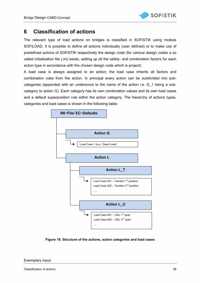
and a default superposition rule within the action category. The hierarchy of actions types,
categories and load cases is shown in the following table:
Figure 16: Structure of the actions, action categories and load cases
Exemplary input:
INI−File/ EC−Defaults
Action G
Load Case 1 (e.g.: Dead Load)
Action L
Action L_T
Load Case 201 – Tandem 1st position
Load Case 202 – Tandem 2nd position
….
Action L_U
Load Case 801 – UDL 1st span
Load Case 802 – UDL 2nd span
….
Bridge Design CABD-Concept
Classification of actions 29
+prog sofiload Head ‘Classification of actions’ $ Traffic Load Actions $ psi-values: acc. to EN 1990/A1 Table A.2.1 $ gamma-values: acc. to EN 1990/A1 Table A.2.4(B) ACT 'L_T' GAMU 1.35 0.00 0.75 0.75 0.00 PART Q EXCL TITL ‘gr1a LM1 TS’ ACT 'L_U' GAMU 1.35 0.00 0.40 0.40 0.00 PART Q EXCL TITL ‘gr1a LM1 UDL’ ACT 'L_F' GAMU 1.35 0.00 0.40 0.40 0.00 PART Q COND TITL ‘gr1aLM1 Foot’ end
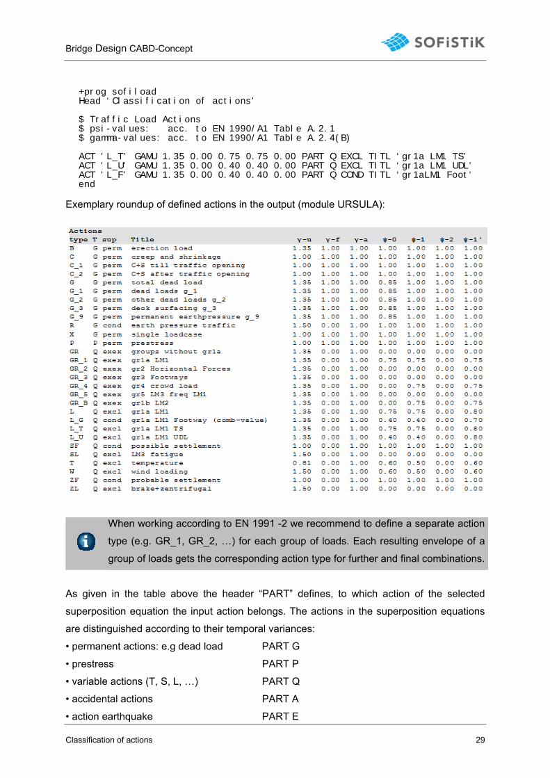
Exemplary roundup of defined actions in the output (module URSULA):
When working according to EN 1991 -2 we recommend to define a separate action
type (e.g. GR_1, GR_2, …) for each group of loads. Each resulting envelope of a
group of loads gets the corresponding action type for further and final combinations.
As given in the table above the header “PART” defines, to which action of the selected
superposition equation the input action belongs. The actions in the superposition equations
are distinguished according to their temporal variances:
• permanent actions: e.g dead load PART G
• prestress PART P
• variable actions (T, S, L, …) PART Q
• accidental actions PART A
• action earthquake PART E
Bridge Design CABD-Concept
Classification of actions 30
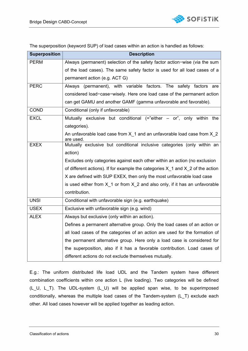
The superposition (keyword SUP) of load cases within an action is handled as follows:
Superposition Description
PERM Always (permanent) selection of the safety factor action−wise (via the sum
of the load cases). The same safety factor is used for all load cases of a
permanent action (e.g. ACT G)
PERC Always (permanent), with variable factors. The safety factors are
considered load−case−wisely. Here one load case of the permanent action
can get GAMU and another GAMF (gamma unfavorable and favorable).
COND Conditional (only if unfavorable)
EXCL Mutually exclusive but conditional (=”either – or”, only within the
categories).
An unfavorable load case from X_1 and an unfavorable load case from X_2 are used.
EXEX Mutually exclusive but conditional inclusive categories (only within an
action)
Excludes only categories against each other within an action (no exclusion
of different actions). If for example the categories X_1 and X_2 of the action
X are defined with SUP EXEX, then only the most unfavorable load case
is used either from X_1 or from X_2 and also only, if it has an unfavorable
contribution.
UNSI Conditional with unfavorable sign (e.g. earthquake)
USEX Exclusive with unfavorable sign (e.g. wind)
ALEX Always but exclusive (only within an action).
Defines a permanent alternative group. Only the load cases of an action or
all load cases of the categories of an action are used for the formation of
the permanent alternative group. Here only a load case is considered for
the superposition, also if it has a favorable contribution. Load cases of
different actions do not exclude themselves mutually.
E.g.: The uniform distributed life load UDL and the Tandem system have different
combination coefficients within one action L (live loading). Two categories will be defined
(L_U, L_T). The UDL-system (L_U) will be applied span wise, to be superimposed
conditionally, whereas the multiple load cases of the Tandem-system (L_T) exclude each
other. All load cases however will be applied together as leading action.
Bridge Design CABD-Concept
Combination rules and superpositioning 31
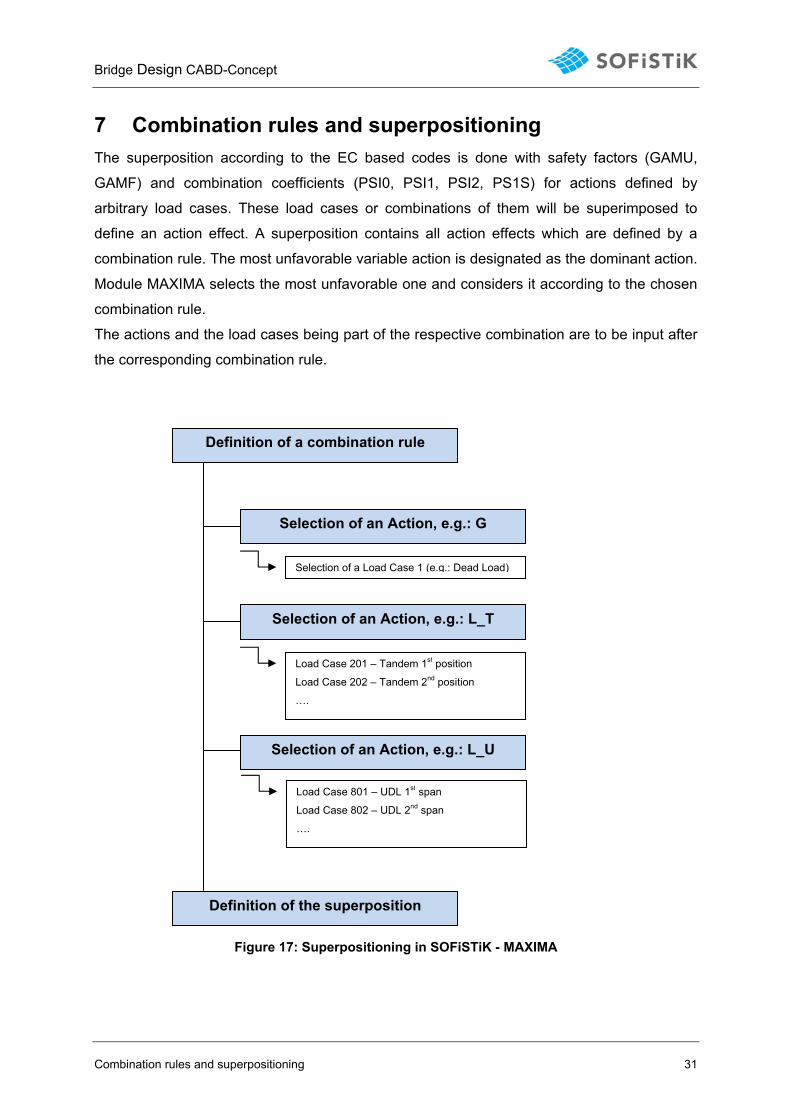
7 Combination rules and superpositioning The superposition according to the EC based codes is done with safety factors (GAMU,
GAMF) and combination coefficients (PSI0, PSI1, PSI2, PS1S) for actions defined by
arbitrary load cases. These load cases or combinations of them will be superimposed to
define an action effect. A superposition contains all action effects which are defined by a
combination rule. The most unfavorable variable action is designated as the dominant action.
Module MAXIMA selects the most unfavorable one and considers it according to the chosen
combination rule.
The actions and the load cases being part of the respective combination are to be input after
the corresponding combination rule.
Figure 17: Superpositioning in SOFiSTiK - MAXIMA
Selection of an Action, e.g.: G
Selection of a Load Case 1 (e.g.: Dead Load)
Selection of an Action, e.g.: L_T
Load Case 201 – Tandem 1st position
Load Case 202 – Tandem 2nd position
….
Selection of an Action, e.g.: L_U
Load Case 801 – UDL 1st span
Load Case 802 – UDL 2nd span
….
Definition of a combination rule
Definition of the superposition
Bridge Design CABD-Concept
Combination rules and superpositioning 32
Within module MAXIMA so called combination rules are defined.
The following predefined combination rules applies all the above mentioned factors and
combination coefficients automatically to each action respectively to each selected load
case.
For checks in ultimate limit state (ULS) we differentiate between:
DESI Ultimate design combination
ACCI Accidental design combination
EARQ Earthquake combination,
For checks in serviceability limit state (SLS) we differentiate between:
PERM Permanent combination
RARE Rare combination
FREQ Frequent combination
NONF Non−frequent combination
For intermediate superposition so called standard combination (STAN) without
safety factors and combination coefficients might be used.
The goal of each superposition is to achieve an envelope for a certain combination rule
(considering safety factors, combination coefficients for leading and accompanying or
coexisting or associated actions). In SOFiSTiK the resulting envelope of each element and
result component (force, displacement, stress,… ) will be stored as a resulting load case
(“load case” or “result case” number). Furthermore the resulting envelope may also be
designated to a type (DESI,ACCI,EARQ,PERM,RARE,FREQ,NONF,STAN, action type, …),
this becomes important when the envelope is subsequently used for a design situation using
the modules AQB (design of beams) or BEMESS (design of shell elements).
The superposition is done for selected elements. An envelope is created for a leading result
component (e.g. internal force) with all associated (resp co-existing) values and stored in a
load case. The default load case numbering scheme is explained in the manual for module
MAXIMA.
Note: A superpositioning in MAXIMA is only available for systems without changes
due to construction changes. MAXIMA supports the load combinations for the final
system only. Wherever construction stages are considered the superposition with

Bridge Design CABD-Concept
Combination rules and superpositioning 33
G+P+C is done using module AQB. This allows to also combine results due to
stage changes.
Bridge Design CABD-Concept
Traffic Loading 34
8 Traffic Loading The goal of the evaluation of moving load effects on bridge structures is to find the most
unfavorable position of the loading for every single element and reaction. Complex load
models and lane arrangements contribute to the fact that the governing loading cannot be
found in an easy way. There a 2 principal approaches in SOFiSTiK to find the most
unfavorable load position:
• Load Stepping: The first approach is to generate a number of representative
loadcases explicitly. Each loadcase contains the load model at distinct positions
along the axis. The loadcases are then calculated and the envelope is obtained with
the superposition module MAXIMA. [Module: SOFiLOAD-V]
• Influence Lines: The second approach is to establish influence lines for forces and
moments of all selected locations within the structure. In a second step the influence
lines are evaluated with the module ELLA by applying the load models. The
envelopes of the results can be directly obtained from this evaluation. [Module: ELLA]
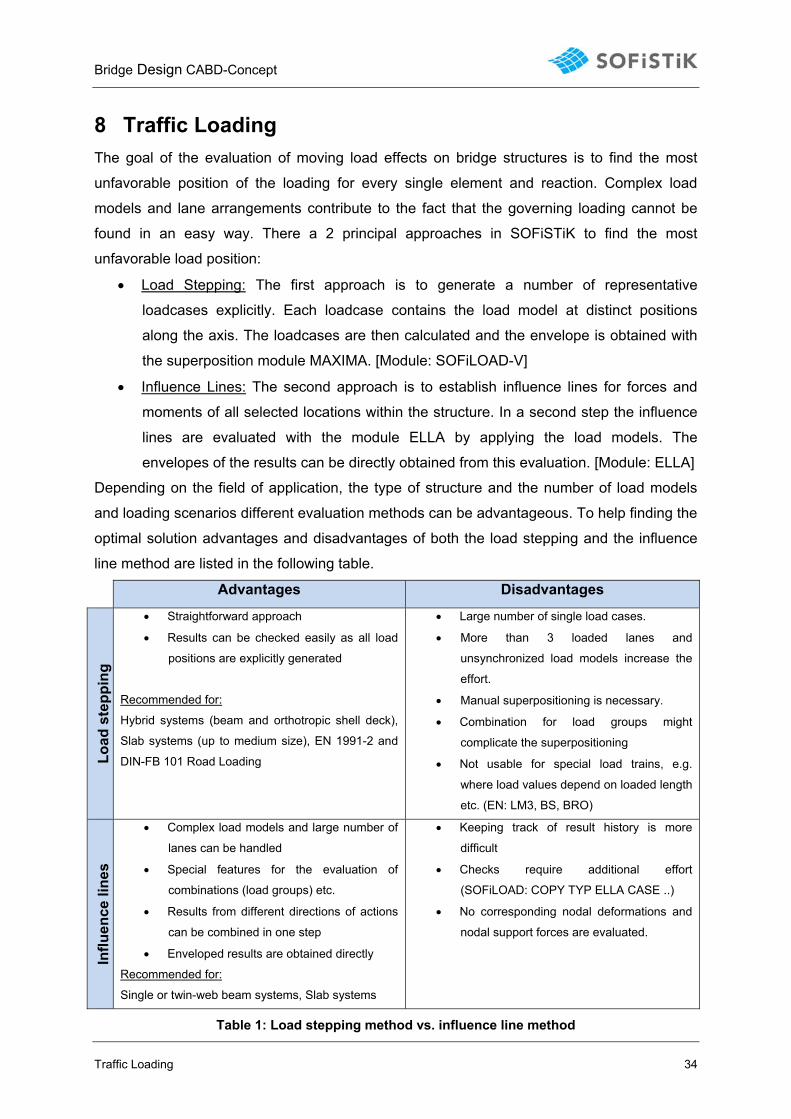
Depending on the field of application, the type of structure and the number of load models
and loading scenarios different evaluation methods can be advantageous. To help finding the
optimal solution advantages and disadvantages of both the load stepping and the influence
line method are listed in the following table.
Advantages Disadvantages
Load
ste
ppin
g
• Straightforward approach
• Results can be checked easily as all load
positions are explicitly generated
Recommended for:
Hybrid systems (beam and orthotropic shell deck),
Slab systems (up to medium size), EN 1991-2 and
DIN-FB 101 Road Loading
• Large number of single load cases.
• More than 3 loaded lanes and
unsynchronized load models increase the
effort.
• Manual superpositioning is necessary.
• Combination for load groups might
complicate the superpositioning
• Not usable for special load trains, e.g.
where load values depend on loaded length
etc. (EN: LM3, BS, BRO)
Influ
ence
line
s
• Complex load models and large number of
lanes can be handled
• Special features for the evaluation of
combinations (load groups) etc.
• Results from different directions of actions
can be combined in one step
• Enveloped results are obtained directly
Recommended for:
Single or twin-web beam systems, Slab systems
• Keeping track of result history is more
difficult
• Checks require additional effort
(SOFiLOAD: COPY TYP ELLA CASE ..)
• No corresponding nodal deformations and
nodal support forces are evaluated.
Table 1: Load stepping method vs. influence line method
Bridge Design CABD-Concept
Traffic Loading 35
8.1 Moving Load Analysis acc. to EN 1991-2
In SOFiSTiK the basis of the traffic load process is the general road/rail axis, described in the
plan view by straight, circular or spiral segments, and in the elevation as straight or quadratic
parabola (c.f. chapter 3). Alternatively a user defined axis with the record GAX in the
modules SOFiLOAD or ELLA can be used for traffic loads. Each axis may have up to 99
lanes with the lane numbers 1-99, defined with the record LANE.
Every single notional lane is loaded separately by a load train. Load trains are defined in
SOFiLOAD. There are two different types of load trains:
• Standard load trains acc. to design codes (using record TRAI) or,
• User defined load trains (user defined using record TRPL, TRBL)
8.1.1 Subdivsion into LANES
Lanes are defined relative to a geometric axis (see above). The lanes may be created
automatically by predefined standard subdivisions or with explicit coordinates. According to
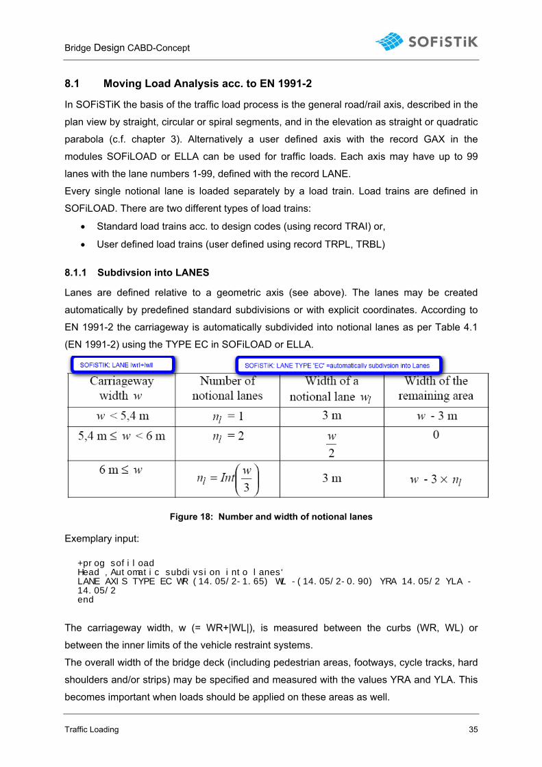
EN 1991-2 the carriageway is automatically subdivided into notional lanes as per Table 4.1
(EN 1991-2) using the TYPE EC in SOFiLOAD or ELLA.
Figure 18: Number and width of notional lanes
Exemplary input: +prog sofiload Head ‚Automatic subdivsion into lanes‘ LANE AXIS TYPE EC WR (14.05/2-1.65) WL -(14.05/2-0.90) YRA 14.05/2 YLA -14.05/2 end
The carriageway width, w (= WR+|WL|), is measured between the curbs (WR, WL) or
between the inner limits of the vehicle restraint systems.
The overall width of the bridge deck (including pedestrian areas, footways, cycle tracks, hard
shoulders and/or strips) may be specified and measured with the values YRA and YLA. This
becomes important when loads should be applied on these areas as well.
Bridge Design CABD-Concept
Traffic Loading 36
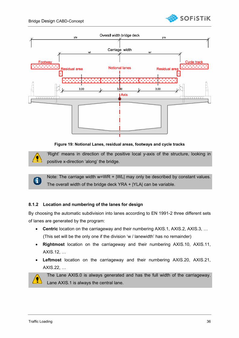
Figure 19: Notional Lanes, residual areas, footways and cycle tracks
‘Right’ means in direction of the positive local y-axis of the structure, looking in
positive x-direction ‘along’ the bridge.
Note: The carriage width w=WR + |WL| may only be described by constant values.
The overall width of the bridge deck YRA + |YLA| can be variable.
8.1.2 Location and numbering of the lanes for design
By choosing the automatic subdivision into lanes according to EN 1991-2 three different sets
of lanes are generated by the program:
• Centric location on the carriageway and their numbering AXIS.1, AXIS.2, AXIS.3, …
(This set will be the only one if the division ‘w / lanewidth’ has no remainder)
• Rightmost location on the carriageway and their numbering AXIS.10, AXIS.11,
AXIS.12, …
• Leftmost location on the carriageway and their numbering AXIS.20, AXIS.21,
AXIS.22, …
The Lane AXIS.0 is always generated and has the full width of the carriageway.
Lane AXIS.1 is always the central lane.
Bridge Design CABD-Concept
Traffic Loading 37
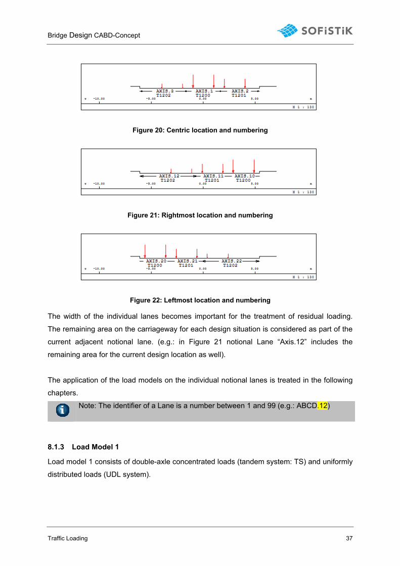
Figure 20: Centric location and numbering
Figure 21: Rightmost location and numbering
Figure 22: Leftmost location and numbering
The width of the individual lanes becomes important for the treatment of residual loading.
The remaining area on the carriageway for each design situation is considered as part of the
current adjacent notional lane. (e.g.: in Figure 21 notional Lane “Axis.12” includes the
remaining area for the current design location as well).
The application of the load models on the individual notional lanes is treated in the following
chapters.
Note: The identifier of a Lane is a number between 1 and 99 (e.g.: ABCD.12)
8.1.3 Load Model 1
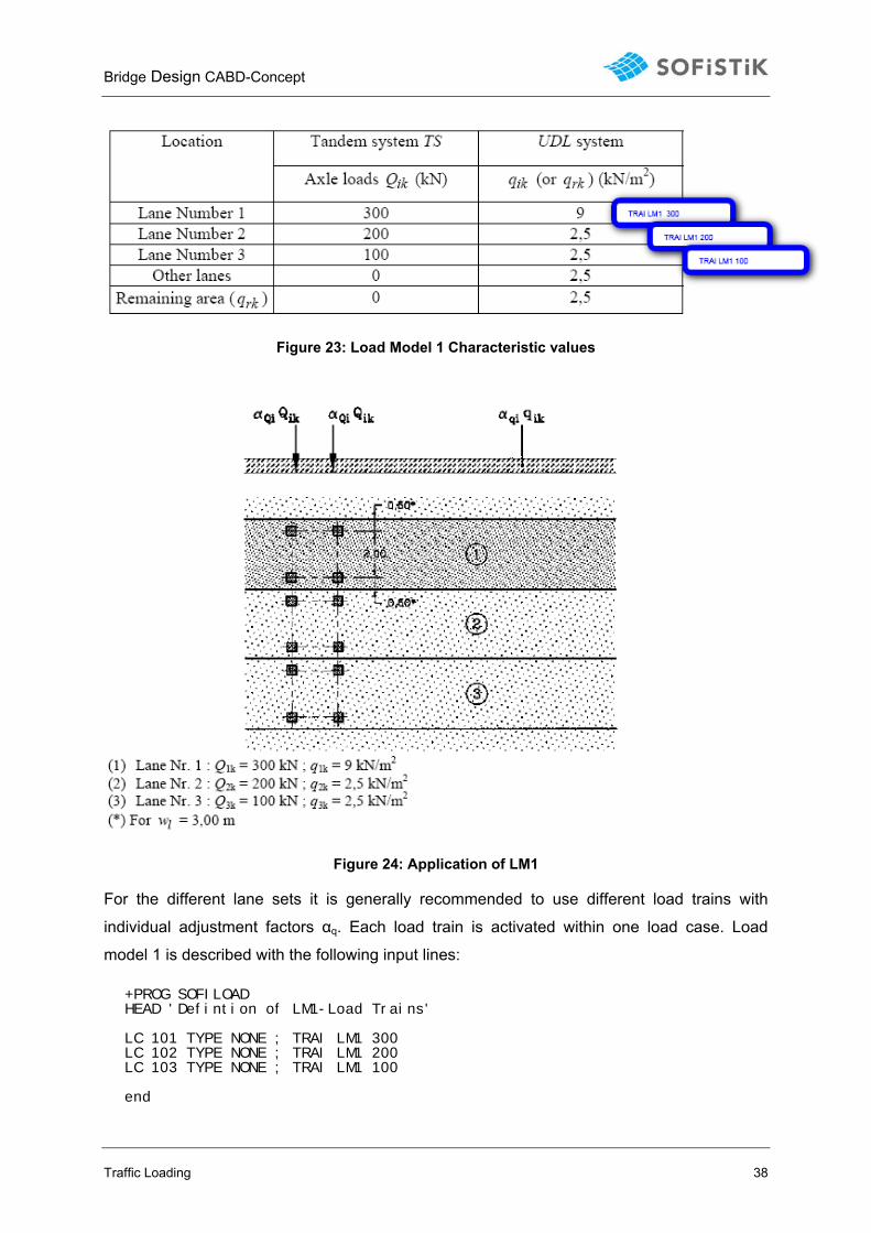
Load model 1 consists of double-axle concentrated loads (tandem system: TS) and uniformly
distributed loads (UDL system).
Bridge Design CABD-Concept
Traffic Loading 38
Figure 23: Load Model 1 Characteristic values
Figure 24: Application of LM1
For the different lane sets it is generally recommended to use different load trains with
individual adjustment factors αq. Each load train is activated within one load case. Load
model 1 is described with the following input lines: +PROG SOFILOAD HEAD 'Defintion of LM1-Load Trains' LC 101 TYPE NONE ; TRAI LM1 300 LC 102 TYPE NONE ; TRAI LM1 200 LC 103 TYPE NONE ; TRAI LM1 100 end
Bridge Design CABD-Concept
Traffic Loading 39
With these commands no loading will be applied to the structure yet. The loading definitions
are saved under a free load case number.
We generally recommend using different load trains with individual adjustment
factors for every single notional lane.
8.1.4 Load Model 2
Load Model 2 consists of a single axle load being applied at any location on the carriageway.
Exemplary input in SOFiLOAD: +PROG SOFILOAD HEAD 'Defintion of LM2-Load Train' LC 104 TYPE NONE ; TRAI LM2 300 end
Load Model 2 is considered when local effects and verifications have to be treated. In this
tutorial Load Model 2 is not analyzed in detail. (i.e. not be selected within ELLA).
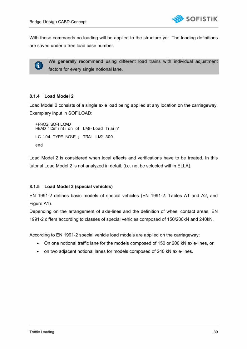
8.1.5 Load Model 3 (special vehicles)
EN 1991-2 defines basic models of special vehicles (EN 1991-2: Tables A1 and A2, and
Figure A1).
Depending on the arrangement of axle-lines and the definition of wheel contact areas, EN
1991-2 differs according to classes of special vehicles composed of 150/200kN and 240kN.
According to EN 1991-2 special vehicle load models are applied on the carriageway:
• On one notional traffic lane for the models composed of 150 or 200 kN axle-lines, or
• on two adjacent notional lanes for models composed of 240 kN axle-lines.
Bridge Design CABD-Concept
Traffic Loading 40
Figure 25: Application of the special vehicles on notional lanes (EN 1991-2: FIGURE A2)
On the other lanes and the remaining area the bridge deck is loaded by Load Model 1 with its
frequent values (ψ1) in addition. There is no loading within a distance of 25 m in front and
behind that vehicle.
The dynamic amplification factor will be considered automatically according to EN 1991-2
φ = 1.40 – 0.002*L ; φ ≥ 1.40
Where the models are assumed to move at low speed, only vertical loads without dynamic
amplification are taken into account. This is achieved by input of an explicit value phi=1.00
for the load train.
Bridge Design CABD-Concept
Traffic Loading 41
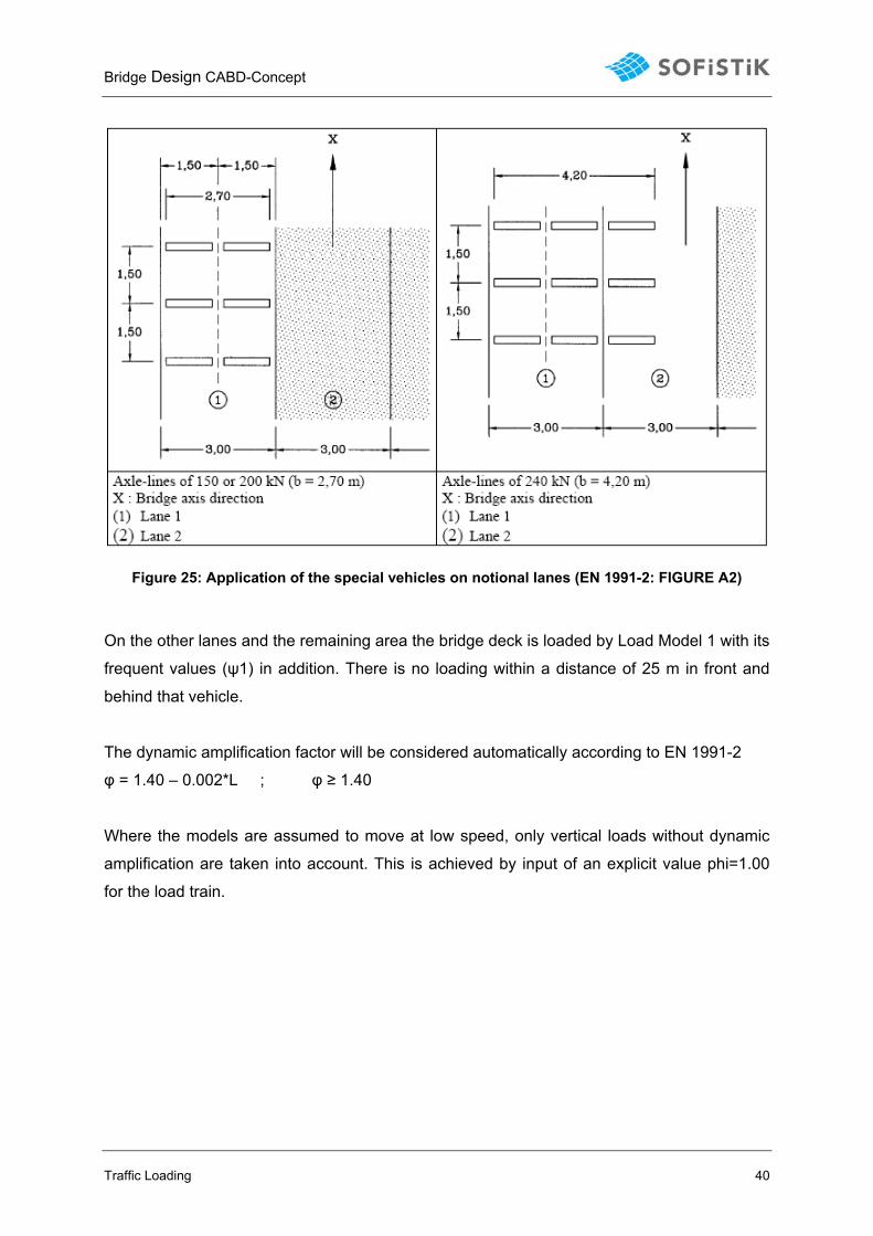
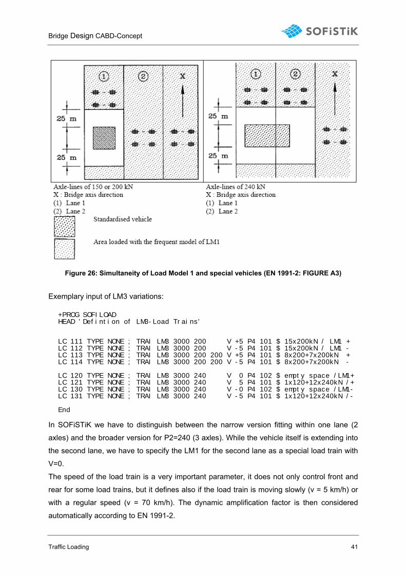
Figure 26: Simultaneity of Load Model 1 and special vehicles (EN 1991-2: FIGURE A3)
Exemplary input of LM3 variations:
+PROG SOFILOAD HEAD 'Defintion of LM3-Load Trains'
LC 111 TYPE NONE ; TRAI LM3 3000 200 V +5 P4 101 $ 15x200kN / LM1 + LC 112 TYPE NONE ; TRAI LM3 3000 200 V -5 P4 101 $ 15x200kN / LM1 - LC 113 TYPE NONE ; TRAI LM3 3000 200 200 V +5 P4 101 $ 8x200+7x200kN + LC 114 TYPE NONE ; TRAI LM3 3000 200 200 V -5 P4 101 $ 8x200+7x200kN - LC 120 TYPE NONE ; TRAI LM3 3000 240 V 0 P4 102 $ empty space /LM1+ LC 121 TYPE NONE ; TRAI LM3 3000 240 V 5 P4 101 $ 1x120+12x240kN /+ LC 130 TYPE NONE ; TRAI LM3 3000 240 V -0 P4 102 $ empty space /LM1- LC 131 TYPE NONE ; TRAI LM3 3000 240 V -5 P4 101 $ 1x120+12x240kN /- End
In SOFiSTiK we have to distinguish between the narrow version fitting within one lane (2
axles) and the broader version for P2=240 (3 axles). While the vehicle itself is extending into
the second lane, we have to specify the LM1 for the second lane as a special load train with
V=0.
The speed of the load train is a very important parameter, it does not only control front and
rear for some load trains, but it defines also if the load train is moving slowly (v = 5 km/h) or
with a regular speed (v = 70 km/h). The dynamic amplification factor is then considered
automatically according to EN 1991-2.
Bridge Design CABD-Concept
Traffic Loading 42
For three axles the speed defines also on which side the third axle is placed. Positive values
will create them on the right side as in the picture above (Figure 26). A definition V=0 will
create the empty space for the second lane only.
By specifying the load case number of a corresponding LM1 load train at P4 this load train is
applied 25 m in front and behind the special vehicle.
To select the relative position to the vehicle in front or behind the sign of the P4 definition will
be taken. As the traffic jam will be behind the vehicle in general positive values will select this
position.
8.1.6 Load Model 4 (crowd loading)
Crowd loading, if relevant, is represented by a Load Model consisting of a uniformly
distributed load (including dynamic amplification) equal to 5 kN/m². +PROG SOFILOAD HEAD 'Defintion of LM4-Load Train' LC 108 TYPE NONE ; TRAI LM4 End
For the application of this load model the definition of the load group is mandatory:
GR3 or GR4 for the area loading and GR0 for the service vehicle.
8.1.7 Fatique Load Model 1
This model is identical to LM1, but the axle loads is reduced by a factor of 0.7, and the
distributed loading by a factor of 0.3.
Exemplary input of FLM1: +PROG SOFILOAD HEAD 'Defintion of FLM1-Load Train' LC 140 TYPE NONE ; TRAI FLM1 300 End
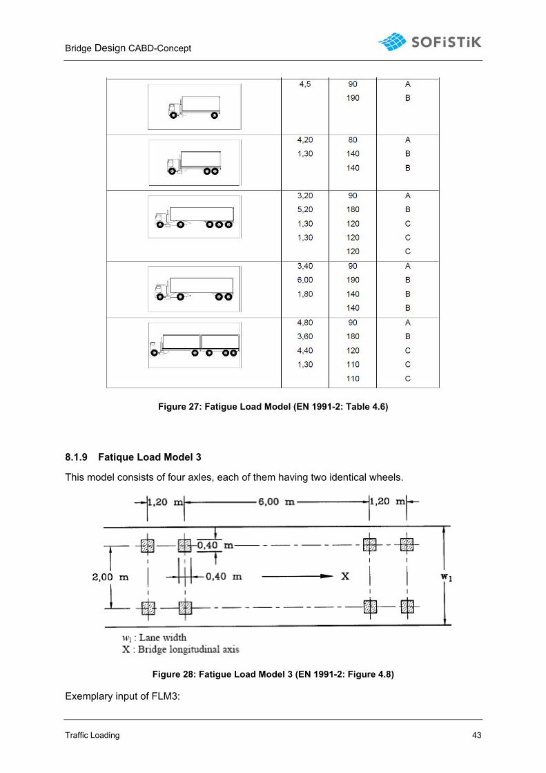
8.1.8 Fatique Load Model 2
Fatigue Load Model 2 consists of a set of idealized lorries, called "frequent" lorries:
Exemplary input of FLM2: +PROG SOFILOAD HEAD 'Defintion of FLM2-Load Train' LC 141 TYPE NONE ; TRAI FLM2 3 End
Bridge Design CABD-Concept
Traffic Loading 43
Figure 27: Fatigue Load Model (EN 1991-2: Table 4.6)
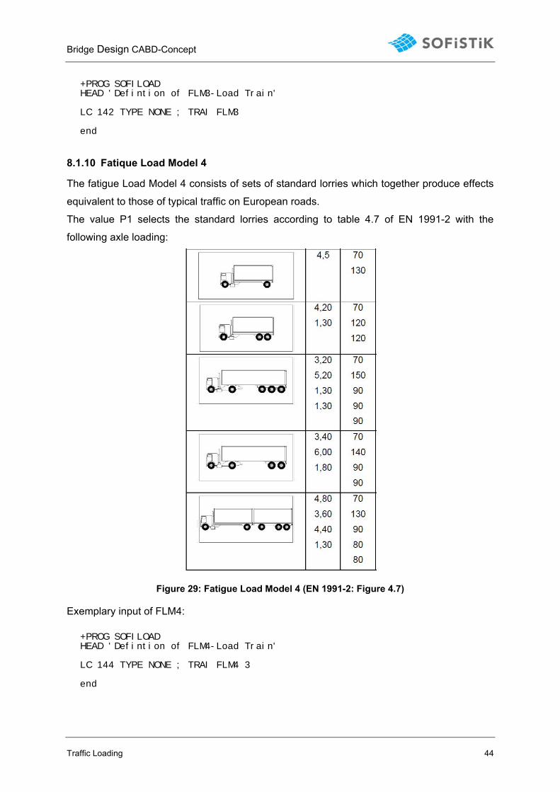
8.1.9 Fatique Load Model 3
This model consists of four axles, each of them having two identical wheels.
Figure 28: Fatigue Load Model 3 (EN 1991-2: Figure 4.8)
Exemplary input of FLM3:
Bridge Design CABD-Concept
Traffic Loading 44
+PROG SOFILOAD HEAD 'Defintion of FLM3-Load Train' LC 142 TYPE NONE ; TRAI FLM3 end
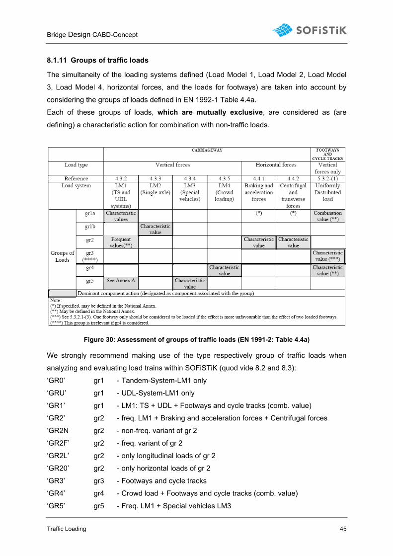
8.1.10 Fatique Load Model 4
The fatigue Load Model 4 consists of sets of standard lorries which together produce effects
equivalent to those of typical traffic on European roads.
The value P1 selects the standard lorries according to table 4.7 of EN 1991-2 with the
following axle loading:
Figure 29: Fatigue Load Model 4 (EN 1991-2: Figure 4.7)
Exemplary input of FLM4: +PROG SOFILOAD HEAD 'Defintion of FLM4-Load Train' LC 144 TYPE NONE ; TRAI FLM4 3 end
Bridge Design CABD-Concept
Traffic Loading 45
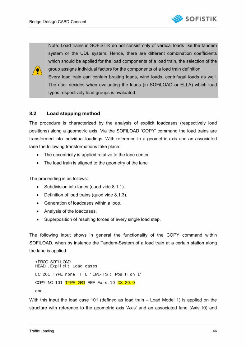
8.1.11 Groups of traffic loads
The simultaneity of the loading systems defined (Load Model 1, Load Model 2, Load Model
3, Load Model 4, horizontal forces, and the loads for footways) are taken into account by
considering the groups of loads defined in EN 1992-1 Table 4.4a.
Each of these groups of loads, which are mutually exclusive, are considered as (are
defining) a characteristic action for combination with non-traffic loads.
Figure 30: Assessment of groups of traffic loads (EN 1991-2: Table 4.4a)
We strongly recommend making use of the type respectively group of traffic loads when
analyzing and evaluating load trains within SOFiSTiK (quod vide 8.2 and 8.3):
‘GR0’ gr1 - Tandem-System-LM1 only
‘GRU’ gr1 - UDL-System-LM1 only
‘GR1’ gr1 - LM1: TS + UDL + Footways and cycle tracks (comb. value)
‘GR2’ gr2 - freq. LM1 + Braking and acceleration forces + Centrifugal forces
‘GR2N gr2 - non-freq. variant of gr 2
‘GR2F’ gr2 - freq. variant of gr 2
‘GR2L’ gr2 - only longitudinal loads of gr 2
‘GR20’ gr2 - only horizontal loads of gr 2
‘GR3’ gr3 - Footways and cycle tracks
‘GR4’ gr4 - Crowd load + Footways and cycle tracks (comb. value)
‘GR5’ gr5 - Freq. LM1 + Special vehicles LM3
Bridge Design CABD-Concept
Traffic Loading 46
Note: Load trains in SOFiSTiK do not consist only of vertical loads like the tandem
system or the UDL system. Hence, there are different combination coefficients
which should be applied for the load components of a load train, the selection of the
group assigns individual factors for the components of a load train definition
Every load train can contain braking loads, wind loads, centrifugal loads as well.
The user decides when evaluating the loads (in SOFiLOAD or ELLA) which load
types respectively load groups is evaluated.
8.2 Load stepping method
The procedure is characterized by the analysis of explicit loadcases (respectively load
positions) along a geometric axis. Via the SOFiLOAD ‘COPY’ command the load trains are
transformed into individual loadings. With reference to a geometric axis and an associated
lane the following transformations take place:
• The eccentricity is applied relative to the lane center
• The load train is aligned to the geometry of the lane
The proceeding is as follows:
• Subdivision into lanes (quod vide 8.1.1).
• Definition of load trains (quod vide 8.1.3).
• Generation of loadcases within a loop.
• Analysis of the loadcases.
• Superposition of resulting forces of every single load step.
The following input shows in general the functionality of the COPY command within
SOFiLOAD, when by instance the Tandem-System of a load train at a certain station along
the lane is applied: +PROG SOFILOAD HEAD ‚Explicit Load cases‘ LC 201 TYPE none TITL 'LM1-TS : Position 1’ COPY NO 101 TYPE GR0 REF Axis.10 DX 20.0 end
With this input the load case 101 (defined as load train – Load Model 1) is applied on the
structure with reference to the geometric axis ‘Axis’ and an associated lane (Axis.10) and
Bridge Design CABD-Concept
Traffic Loading 47
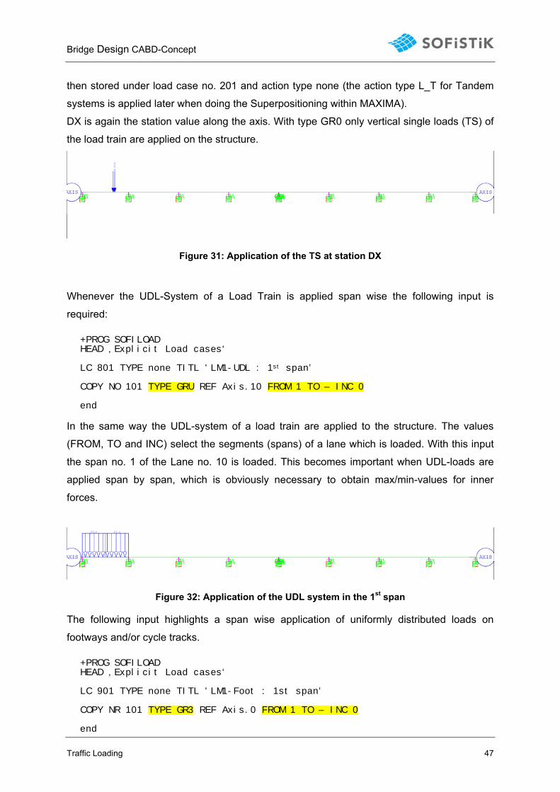
then stored under load case no. 201 and action type none (the action type L_T for Tandem
systems is applied later when doing the Superpositioning within MAXIMA).
DX is again the station value along the axis. With type GR0 only vertical single loads (TS) of
the load train are applied on the structure.
Figure 31: Application of the TS at station DX
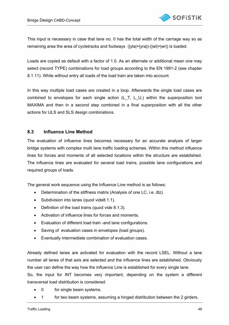
Whenever the UDL-System of a Load Train is applied span wise the following input is
required: +PROG SOFILOAD HEAD ‚Explicit Load cases‘ LC 801 TYPE none TITL 'LM1-UDL : 1st span’ COPY NO 101 TYPE GRU REF Axis.10 FROM 1 TO – INC 0 end
In the same way the UDL-system of a load train are applied to the structure. The values
(FROM, TO and INC) select the segments (spans) of a lane which is loaded. With this input
the span no. 1 of the Lane no. 10 is loaded. This becomes important when UDL-loads are
applied span by span, which is obviously necessary to obtain max/min-values for inner
forces.
Figure 32: Application of the UDL system in the 1st span
The following input highlights a span wise application of uniformly distributed loads on
footways and/or cycle tracks. +PROG SOFILOAD HEAD ‚Explicit Load cases‘ LC 901 TYPE none TITL 'LM1-Foot : 1st span’ COPY NR 101 TYPE GR3 REF Axis.0 FROM 1 TO – INC 0 end
Bridge Design CABD-Concept
Traffic Loading 48
This input is necessary in case that lane no. 0 has the total width of the carriage way so as
remaining area the area of cycletracks and footways (|yla|+|yra|)-(|wl|+|wr|) is loaded.
Loads are copied as default with a factor of 1.0. As an alternate or additional mean one may
select (record TYPE) combinations for load groups according to the EN 1991-2 (see chapter
8.1.11). While without entry all loads of the load train are taken into account.
In this way multiple load cases are created in a loop. Afterwards the single load cases are
combined to envelopes for each single action (L_T, L_U,) within the superposition tool
MAXIMA and then in a second step combined in a final superposition with all the other
actions for ULS and SLS design combinations.
8.3 Influence Line Method
The evaluation of influence lines becomes necessary for an accurate analysis of larger
bridge systems with complex multi lane traffic loading schemes. Within this method influence
lines for forces and moments of all selected locations within the structure are established.
The influence lines are evaluated for several load trains, possible lane configurations and
required groups of loads.
The general work sequence using the Influence Line method is as follows:
• Determination of the stiffness matrix (Analysis of one LC, i.e. dlz).
• Subdivision into lanes (quod vide8.1.1).
• Definition of the load trains (quod vide 8.1.3).
• Activation of influence lines for forces and moments.
• Evaluation of different load train -and lane configurations.
• Saving of evaluation cases in envelopes (load groups).
• Eventually intermediate combination of evaluation cases.
Already defined lanes are activated for evaluation with the record LSEL. Without a lane
number all lanes of that axis are selected and the influence lines are established. Obviously
the user can define the way how the influence Line is established for every single lane.
So, the input for INT becomes very important, depending on the system a different
transversal load distribution is considered:
• 0 for single beam systems.
• 1 for two beam systems, assuming a hinged distribution between the 2 girders.
Bridge Design CABD-Concept
Traffic Loading 49
• 2 for two beam systems, assuming a rigid distribution between the 2 girders.
• 3,5,7,9 for slab systems a transverse influence lines on shell elements are
established, where the numbers of load points in transverse direction are specified.
For spatial systems we strongly recommend to make use of the parameter DZ, which defines
the depth under the lane which will be investigated for node-sequences. Nodes above the
lane axis (negative z axis) are never considered.
One may specify for which inner forces we get an envelope. For each inner force the load
case no. for the maximum and minimum values are defined. The resulting LC no. of the
envelope in the Database = BASE no. + LMAX/LMIN.
In the same way as for the load stepping method different cases (multi lane traffic loading
schemes) are investigated within ELLA. The envelope of several evaluation cases is stored
with the record SAVE in a so called saving case, by specifying base-number and action type
for the results. Each case gets an identification number and assigns a load train to an
individual lane. With input of GRP one specifies the groups of traffic loads according to EN
1991-2, which is evaluated from the load train.
All evaluation cases in a saving case are mutually exclusive; the maximum of these will be
carried out by ELLA.
The command SHOW is used to represent influence lines for inner forces and moments with
the corresponding load position in a lane for a given element (e.g. beam element 40040).
The synchronization with secondary lanes should not be applied; this is controlled for each
lane with the record SYNC OFF in POSL.
The double axle is applied only in total. Thus all loads of the axles are set to be applied even
if favorable.
Bridge Design CABD-Concept
Traffic Loading 50
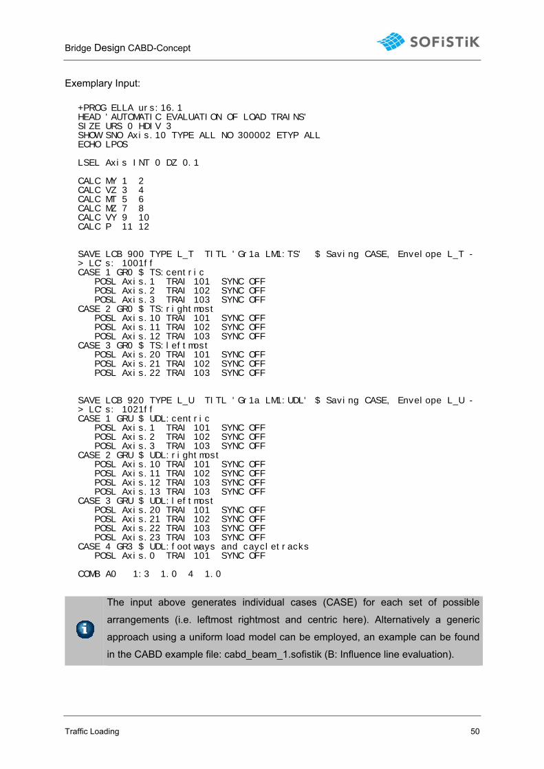
Exemplary Input: +PROG ELLA urs:16.1 HEAD 'AUTOMATIC EVALUATION OF LOAD TRAINS' SIZE URS 0 HDIV 3 SHOW SNO Axis.10 TYPE ALL NO 300002 ETYP ALL ECHO LPOS LSEL Axis INT 0 DZ 0.1 CALC MY 1 2 CALC VZ 3 4 CALC MT 5 6 CALC MZ 7 8 CALC VY 9 10 CALC P 11 12 SAVE LCB 900 TYPE L_T TITL 'Gr1a LM1:TS' $ Saving CASE, Envelope L_T -> LC's: 1001ff CASE 1 GR0 $ TS:centric POSL Axis.1 TRAI 101 SYNC OFF POSL Axis.2 TRAI 102 SYNC OFF POSL Axis.3 TRAI 103 SYNC OFF CASE 2 GR0 $ TS:rightmost POSL Axis.10 TRAI 101 SYNC OFF POSL Axis.11 TRAI 102 SYNC OFF POSL Axis.12 TRAI 103 SYNC OFF CASE 3 GR0 $ TS:leftmost POSL Axis.20 TRAI 101 SYNC OFF POSL Axis.21 TRAI 102 SYNC OFF POSL Axis.22 TRAI 103 SYNC OFF SAVE LCB 920 TYPE L_U TITL 'Gr1a LM1:UDL' $ Saving CASE, Envelope L_U -> LC's: 1021ff CASE 1 GRU $ UDL:centric POSL Axis.1 TRAI 101 SYNC OFF POSL Axis.2 TRAI 102 SYNC OFF POSL Axis.3 TRAI 103 SYNC OFF CASE 2 GRU $ UDL:rightmost POSL Axis.10 TRAI 101 SYNC OFF POSL Axis.11 TRAI 102 SYNC OFF POSL Axis.12 TRAI 103 SYNC OFF POSL Axis.13 TRAI 103 SYNC OFF CASE 3 GRU $ UDL:leftmost POSL Axis.20 TRAI 101 SYNC OFF POSL Axis.21 TRAI 102 SYNC OFF POSL Axis.22 TRAI 103 SYNC OFF POSL Axis.23 TRAI 103 SYNC OFF CASE 4 GR3 $ UDL:footways and caycletracks POSL Axis.0 TRAI 101 SYNC OFF COMB A0 1:3 1.0 4 1.0
The input above generates individual cases (CASE) for each set of possible
arrangements (i.e. leftmost rightmost and centric here). Alternatively a generic
approach using a uniform load model can be employed, an example can be found
in the CABD example file: cabd_beam_1.sofistik (B: Influence line evaluation).
Bridge Design CABD-Concept
Traffic Loading 51
8.4 Highway bridge loading acc. to BS 5400 (BD37/01)
The basic features of a moving load analysis described in the previous sections is be applied
to various other traffic loading scenarios. In the following the traffic loading according to the
composite version of BS 5400 (Volume 1 Section 3 and Appendix A) is considered.
Due to dependency of the HA type UDL loading on loaded length and variable
overall length of the HB vehicle a correct evaluation is only possible using influence
lines in module ELLA.
8.4.1 Subdivision into notional lanes
Similar to the subdivision scheme of the Eurocode, an automatic subdivision of the
carriageway acc. to BS 5400 clause 3.2.9 is activated with LANE TYPE BS. The exemplary
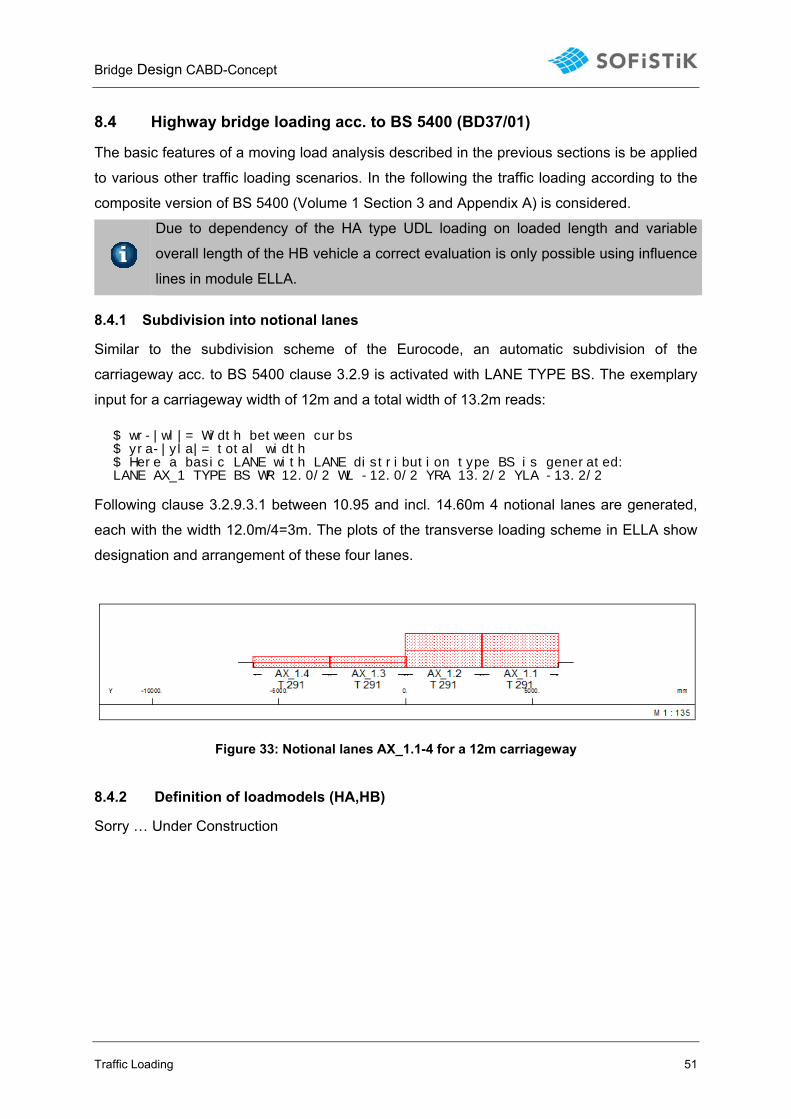
input for a carriageway width of 12m and a total width of 13.2m reads:
$ wr-|wl|= Width between curbs $ yra-|yla|= total width $ Here a basic LANE with LANE distribution type BS is generated: LANE AX_1 TYPE BS WR 12.0/2 WL -12.0/2 YRA 13.2/2 YLA -13.2/2
Following clause 3.2.9.3.1 between 10.95 and incl. 14.60m 4 notional lanes are generated,
each with the width 12.0m/4=3m. The plots of the transverse loading scheme in ELLA show
designation and arrangement of these four lanes.
Figure 33: Notional lanes AX_1.1-4 for a 12m carriageway
8.4.2 Definition of loadmodels (HA,HB)
Sorry … Under Construction
Bridge Design CABD-Concept
Construction stages 52
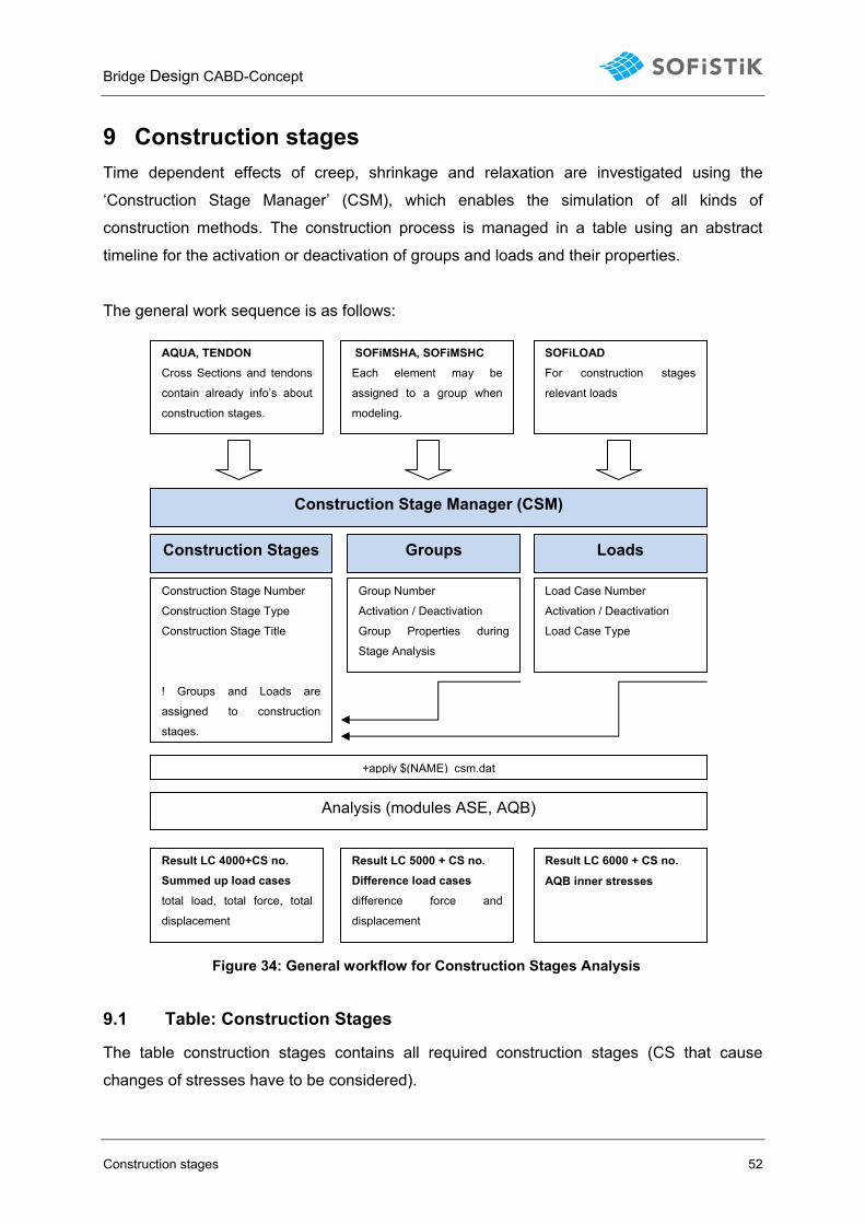
9 Construction stages Time dependent effects of creep, shrinkage and relaxation are investigated using the
‘Construction Stage Manager’ (CSM), which enables the simulation of all kinds of
construction methods. The construction process is managed in a table using an abstract
timeline for the activation or deactivation of groups and loads and their properties.
The general work sequence is as follows:
9.1 Table: Construction Stages
The table construction stages contains all required construction stages (CS that cause
changes of stresses have to be considered).
Construction Stages
SOFiMSHA, SOFiMSHCEach element may be
assigned to a group when
modeling.
Groups Loads
SOFiLOADFor construction stages
relevant loads
AQUA, TENDON Cross Sections and tendons
contain already info’s about
construction stages.
Group Number
Activation / Deactivation
Group Properties during
Stage Analysis
Load Case Number
Activation / Deactivation
Load Case Type
Construction Stage Number
Construction Stage Type
Construction Stage Title
! Groups and Loads are
assigned to construction
stages.
Construction Stage Manager (CSM)
Analysis (modules ASE, AQB)
Result LC 5000 + CS no.Difference load cases difference force and
displacement
Result LC 6000 + CS no.
AQB inner stresses
Result LC 4000+CS no. Summed up load cases total load, total force, total
displacement
+apply $(NAME)_csm.dat
Figure 34: General workflow for Construction Stages Analysis
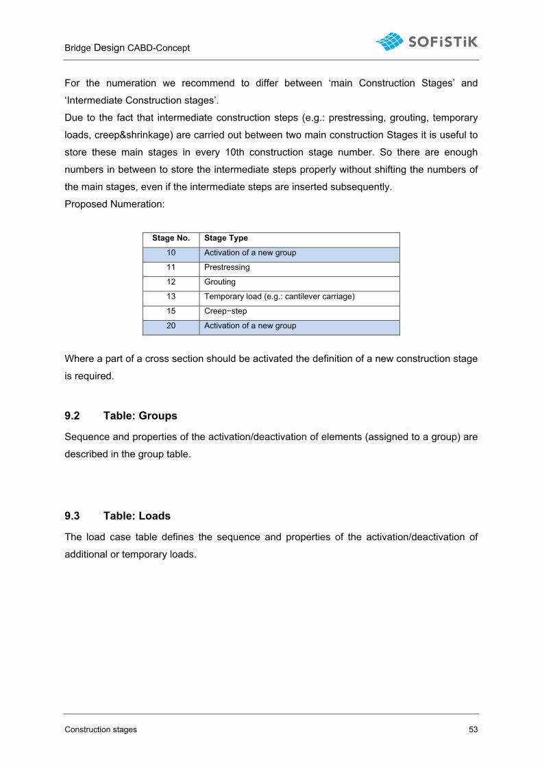
Bridge Design CABD-Concept
Construction stages 53
For the numeration we recommend to differ between ‘main Construction Stages’ and
‘Intermediate Construction stages’.
Due to the fact that intermediate construction steps (e.g.: prestressing, grouting, temporary
loads, creep&shrinkage) are carried out between two main construction Stages it is useful to
store these main stages in every 10th construction stage number. So there are enough
numbers in between to store the intermediate steps properly without shifting the numbers of
the main stages, even if the intermediate steps are inserted subsequently.
Proposed Numeration:
Stage No. Stage Type
10 Activation of a new group
11 Prestressing
12 Grouting
13 Temporary load (e.g.: cantilever carriage)
15 Creep−step
20 Activation of a new group
Where a part of a cross section should be activated the definition of a new construction stage
is required.
9.2 Table: Groups
Sequence and properties of the activation/deactivation of elements (assigned to a group) are
described in the group table.
9.3 Table: Loads
The load case table defines the sequence and properties of the activation/deactivation of
additional or temporary loads.
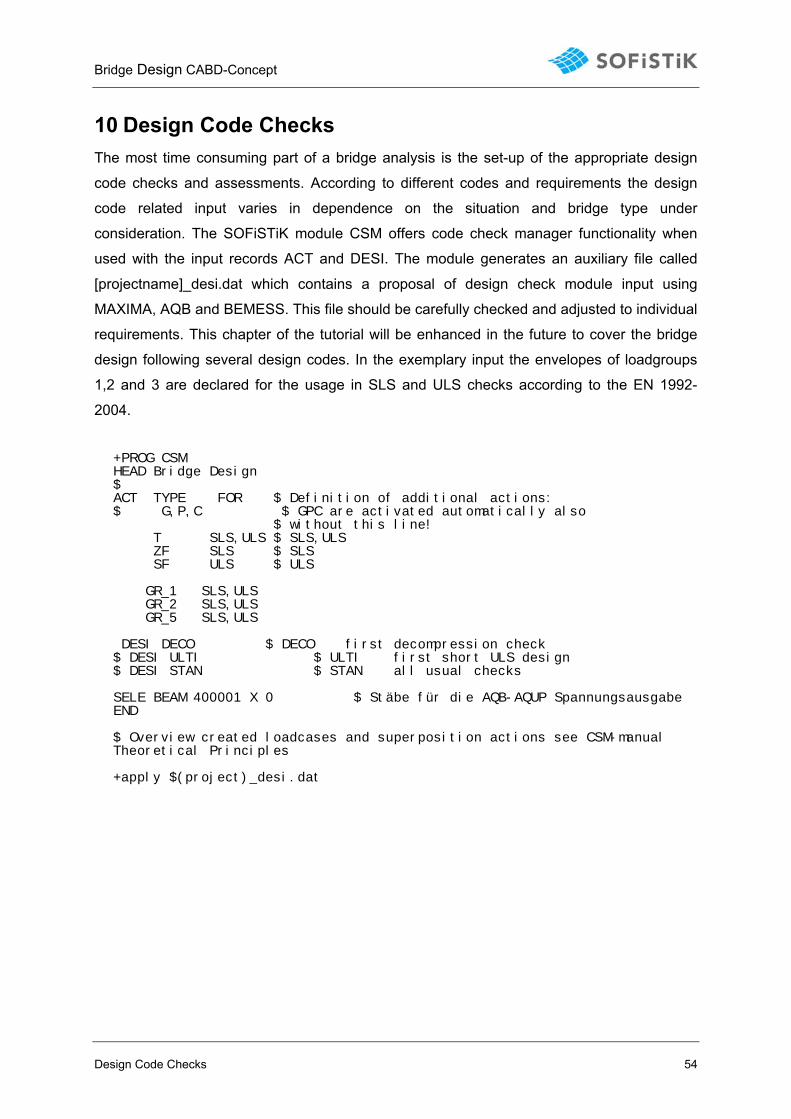
Bridge Design CABD-Concept
Design Code Checks 54
10 Design Code Checks The most time consuming part of a bridge analysis is the set-up of the appropriate design
code checks and assessments. According to different codes and requirements the design
code related input varies in dependence on the situation and bridge type under
consideration. The SOFiSTiK module CSM offers code check manager functionality when
used with the input records ACT and DESI. The module generates an auxiliary file called
[projectname]_desi.dat which contains a proposal of design check module input using
MAXIMA, AQB and BEMESS. This file should be carefully checked and adjusted to individual
requirements. This chapter of the tutorial will be enhanced in the future to cover the bridge
design following several design codes. In the exemplary input the envelopes of loadgroups
1,2 and 3 are declared for the usage in SLS and ULS checks according to the EN 1992-
2004.
+PROG CSM HEAD Bridge Design $ ACT TYPE FOR $ Definition of additional actions: $ G,P,C $ GPC are activated automatically also $ without this line! T SLS,ULS $ SLS,ULS ZF SLS $ SLS SF ULS $ ULS GR_1 SLS,ULS GR_2 SLS,ULS GR_5 SLS,ULS DESI DECO $ DECO first decompression check $ DESI ULTI $ ULTI first short ULS design $ DESI STAN $ STAN all usual checks SELE BEAM 400001 X 0 $ Stäbe für die AQB-AQUP Spannungsausgabe END $ Overview created loadcases and superposition actions see CSM-manual Theoretical Principles +apply $(project)_desi.dat
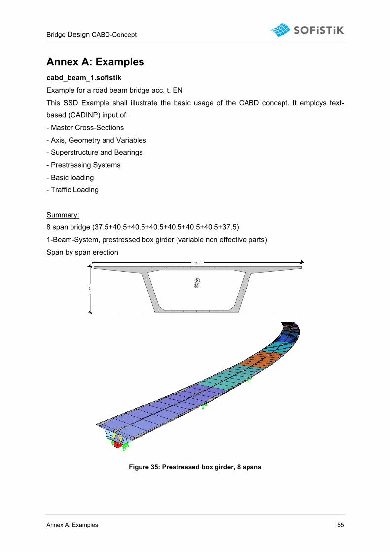
Bridge Design CABD-Concept
Annex A: Examples 55
Annex A: Examples cabd_beam_1.sofistik Example for a road beam bridge acc. t. EN
This SSD Example shall illustrate the basic usage of the CABD concept. It employs text-
based (CADINP) input of:
- Master Cross-Sections
- Axis, Geometry and Variables
- Superstructure and Bearings
- Prestressing Systems
- Basic loading
- Traffic Loading
Summary:
8 span bridge (37.5+40.5+40.5+40.5+40.5+40.5+40.5+37.5)
1-Beam-System, prestressed box girder (variable non effective parts)
Span by span erection
Figure 35: Prestressed box girder, 8 spans
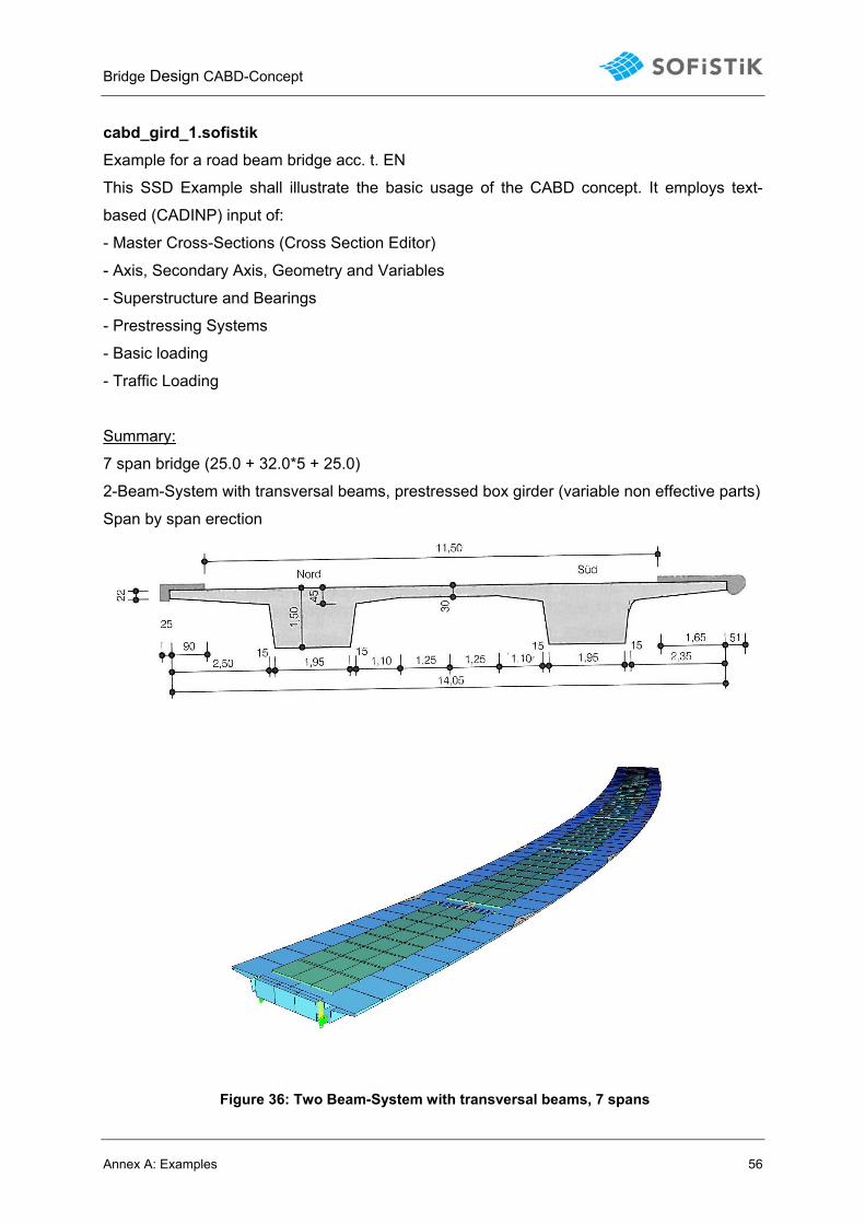
Bridge Design CABD-Concept
Annex A: Examples 56
cabd_gird_1.sofistik Example for a road beam bridge acc. t. EN
This SSD Example shall illustrate the basic usage of the CABD concept. It employs text-
based (CADINP) input of:
- Master Cross-Sections (Cross Section Editor)
- Axis, Secondary Axis, Geometry and Variables
- Superstructure and Bearings
- Prestressing Systems
- Basic loading
- Traffic Loading
Summary:
7 span bridge (25.0 + 32.0*5 + 25.0)
2-Beam-System with transversal beams, prestressed box girder (variable non effective parts)
Span by span erection
Figure 36: Two Beam-System with transversal beams, 7 spans