Tutorial: Big Data Algorithms and Applications …kpzhang/tutorial/amcis2014_files/...Tutorial: Big Data Algorithms and Applications Under Hadoop KUNPENG ZHANG SIDDHARTHA BHATTACHARYYA

Tutorial: Big Data Algorithms and Applications Under Hadoop

KUNPENG ZHANG SIDDHARTHA BHATTACHARYYA

http://kzhang6.people.uic.edu/tutorial/amcis2014.html August 7, 2014

Schedule

I. Introduction to big data (8:00 – 8:30) II. Hadoop and MapReduce (8:30 – 9:45) III. Coffee break (9:45 – 10:00) IV. Distributed algorithms and applications (10:00 – 11:40) V. Conclusion (11:40 – 12:00)

I. Introduction to big data

I. Introduction to big data

•  What is big data

•  Why big data matters to you •  10 use cases of big data analytics

•  Techniques for analyzing big data

What is big data

•  Big data is a blanket term for any types of data sets so large and complex that it becomes difficult to process using on-hand data management tools or traditional data processing applications. [From Wikipedia]

5 Vs of big data

•  To get better understanding of what big data is, it is often described using 5 Vs.

Volume

Velocity

Value

Veracity

Variety

We see increasing volume of data, that grow at exponential rates

Volume refers to the vast amount of data generated every second. We are not talking about Terabytes but Zettabytes or Brontobytes. If we take all the data generated in the world between the beginning of time and 2008, the same amount of data will soon be generated every minute. This makes most data sets too large to store and analyze using traditional database technology. New big data tools use distributed systems so we can store and analyze data across databases that are dotted around everywhere in the world.

Volume

Velocity

Value

Veracity

Variety

We see increasing velocity (or speed) at which data changes, travels, or increases

Velocity refers to the speed at which new data is generated and the speed at which data moves around. Just think of social media messages going viral in seconds. Technology now allows us to analyze the data while it is being generated (sometimes referred to as it in-memory analytics), without ever putting into databases.

Volume

Velocity

Value

Veracity

Variety

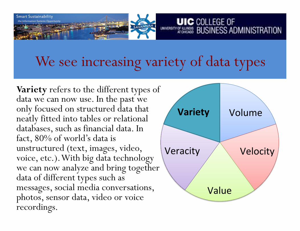
We see increasing variety of data types

Variety refers to the different types of data we can now use. In the past we only focused on structured data that neatly fitted into tables or relational databases, such as financial data. In fact, 80% of world’s data is unstructured (text, images, video, voice, etc.). With big data technology we can now analyze and bring together data of different types such as messages, social media conversations, photos, sensor data, video or voice recordings.

Volume

Velocity

Value

Veracity

Variety

We see increasing veracity (or accuracy) of data

Veracity refers to messiness or trustworthiness of data. With many forms of big data quality and accuracy are less controllable (just think Twitter posts with hash tags, abbreviations, typos and colloquial speech as well as the reliability and accuracy of content) but technology now allows us to work with this type of data.

Volume

Velocity

Value

Veracity

Variety

Value – The most important V of all!

There is another V to take into account when looking at big data: Value. Having access to big data is no good unless we can turn it into value. Companies are starting to generate amazing value from their big data.

Volume

Velocity

Value

Veracity

Variety

Introduction to big data




Big data is more prevalent than you think

Big data formats

Competitive advantages gained through big data

Big data job postings





1. Understanding and targeting customers •  Big data is used to better

understand customers and their behaviors and preferences. –  Target: very accurately predict

when one of their customers will expect a baby;

–  Wal-Mart can predict what products will sell;

–  Car insurance companies understand how well their customers actually drive;

–  Obama use big data analytics to win 2012 presidential election campaign.

Predic0ve models

Social media data

Browser logs

Sensor data

Text analy0cs

2. Understanding and optimizing business processes

•  Retailers are able to optimize their stock based on predictions generated from social media data, web search trends, and weather forecasts;

•  Geographic positioning and radio frequency identification sensors are used to track goods or delivery vehicles and optimize routes by integrating live traffic data, etc.

3. Personal quantification and performance optimization

•  The Jawbone armband collects data on our calorie consumption, activity levels, and our sleep patterns and analyze such volumes of data to bring entirely new insights that it can feed back to individual users;

•  Most online dating sites apply big data tools and algorithms to find us the most appropriate matches.

4. Improving healthcare and public health

•  Big data techniques are already being used to monitor babies in a specialist premature and sick baby unit;

•  Big data analytics allow us to monitor and predict the developments of epidemics and disease outbreaks;

•  By recording and analyzing every heart beat and breathing pattern of every baby, infections can be predicted 24 hours before any physical symptoms appear.

5. Improving sports performance

•  Use video analytics to track the performance of every player;

•  Use sensor technology in sports equipment to allow us to get feedback on games;

•  Use smart technology to track athletes outside of the sporting environment: nutrition, sleep, and social media conversation.

6. Improving science and research

•  CERN, the Swiss nuclear physics lab with its Large Hadron Collider, the world’s largest and most powerful particle accelerator is using thousands of computers distributed across 150 data centers worldwide to unlock the secrets of our universe by analyzing its 30 petabytes of data.

7. Optimizing machine and device performance

•  Google self-driving car: the Toyota Prius is fitted with cameras, GPS, powerful computers and sensors to safely drive without the intervention of human beings;

•  Big data tools are also used to optimize energy grids using data from smart meters.

8. Improving security and law enforcement

•  National Security Agency (NSA) in the U.S. uses big data analytics to foil terrorist plots (and maybe spy on us);

•  Police forces use big data tools to catch criminals and even predict criminal activity;

•  Credit card companies use big data to detect fraudulent transactions.

9. Improving and optimizing cities and countries

•  Smart cities optimize traffic flows based on real time traffic information as well as social media and weather data.

10. Financial trading

•  The majority of equity trading now takes place via data algorithms that increasingly take into account signals from social media networks and news websites to make, buy and sell decisions in split seconds (High-Frequency Trading, HFT).





Techniques and their applications

•  Association rule mining: market basket analysis •  Classification: prediction of customer buying decisions •  Cluster analysis: segmenting consumers into groups •  Crowdsourcing: collecting data from community •  Data fusion and data integration: social media data

combined with real-time sales data to determine what effect a marketing campaign is having on customer sentiment and purchasing behavior


•  Ensemble learning •  Genetic algorithms: job scheduling in manufacturing

and optimizing the performance of an investment portfolio •  Neural networks: identify fraudulent insurance claims •  Natural language processing: sentiment analysis

•  Network analysis: identifying key opinion leaders to target for marketing and identifying bottlenecks in enterprise information flows


•  Regression: forecasting sales volumes based on various market and economic variables

•  Time series analysis: hourly value of a stock market index or the number of patients diagnosed with a given condition every day

•  Visualization: understand and improve results of big data analyses

Big data tools

•  Big Table by Google •  MapReduce by Google •  Cassandra by Apache •  Dynamo by Amazon •  Hbase by Apache •  Hadoop by Apache

Visualization tools

•  D3.js: http://d3js.org/ •  Tag cloud: http://tagcrowd.com/ •  Clustergram:

http://www.schonlau.net/clustergram.html •  History flow: http://hint.fm/projects/historyflow/

•  R: http://www.r-project.org/ •  Network visualization (Gephi): http://gephi.github.io/

Schedule


II. Hadoop and MapReduce

Hadoop and MapReduce

•  What is Hadoop •  Hadoop architecture •  What is MapReduce •  Hadoop installation and configuration •  Hadoop shell commands •  MapReduce programming (word-count example)

Assumptions and goals

•  Hardware failure •  Streaming data access •  Large data sets •  Simple coherency model (write-once-read-many access) •  Moving computation is cheaper than moving data •  Portability Across Heterogeneous Hardware and Software

Platforms

What is Hadoop?

•  Hadoop is a software framework for distributed processing of large datasets across large clusters of computers.

•  Hadoop is based on a simple programming model called MapReduce.

•  Hadoop is based on a simple data model, any data will fit. •  Hadoop framework consists on two main layers: – Distributed file system (HDFS) – Execution engine (MapReduce)

A multi-node Hadoop cluster

•  MapReduce layer: computing and programming

•  HDFS layer: file storage



HDFS architecture

HDFS architecture

•  HDFS has master/slave architecture. •  An HDFS cluster consists of a single NameNode, a master

server that manages the file system namespace and regulates access to files by clients.

•  There are a number of DataNodes, usually one per node in the cluster, which manage storage attached to the nodes that they run on.

•  HDFS exposes a file system namespace and allows user data to be stored in files. Internally, a file is split into one or more blocks and these blocks are stored in a set of DataNodes.

NameNode and DataNodes

•  The NameNode executes file system namespace operations like opening, closing, and renaming files and directories.

•  The NameNode also determines the mapping of blocks to DataNodes.

•  The DataNodes are responsible for serving read and write requests from the file system’s clients.

•  The DataNodes also perform block creation, deletion, and replication upon instruction from the NameNode.

•  The NameNode periodically receives a Heartbeat and a Blockreport from each of the DataNodes in the cluster. Receipt of a Heartbeat implies that the DataNode is functioning properly. A Blockreport contains a list of all blocks on a DataNode.

Data replication

•  HDFS is designed to reliably store very large files across machines in a large cluster. It stores each file as a sequence of blocks.

•  All blocks in a file except the last block are the same size. •  The blocks of a file are replicated for fault tolerance. •  The block size (default: 64M) and replication factor

(default: 3) are configurable per file.

Data replication

Placement policy

•  Where to put a given block? (3 copies by default) – Frist copy is written to the node creating the file (write

affinity) – Second copy is written to a DataNode within the same rack – Third copy is written to a DataNode in a different rack – Objectives: load balancing, fast access, fault tolerance



MapReduce definition

•  MapReduce is a programming model and an associated implementation for processing and generating large data sets with a parallel, distributed algorithm on a cluster.

MapReduce framework

•  Per cluster node: – Single JobTracker per master •  Responsible for scheduling the

jobs’ component tasks on the slaves •  Monitor slave progress •  Re-execute failed tasks

– Single TaskTracker per slave •  Execute the task as directed by

the master

MapReduce core functionality (I)

•  Code usually written in Java - though it can be written in other languages with the Hadoop Streaming API.

•  Two fundamental components: – Map step

•  Master node takes large problem and slices it into smaller sub problems; distributes these to worker nodes.

•  Worker node may do this again if necessary. •  Worker processes smaller problem and hands back to master.

– Reduce step •  Master node takes the answers to the sub problems and combines them in a

predefined way to get the output/answer to original problem.

MapReduce core functionality (II)

•  Data flow beyond the two key components (map and reduce): –  Input reader – divides input into appropriate size splits which get

assigned to a Map function. – Map function – maps file data/split to smaller, intermediate <key,

value> pairs. –  Partition function – finds the correct reducer: given the key and

number of reducers, returns the desired reducer node. (optional) – Compare function – input from the Map intermediate output is

sorted according to the compare function. (optional) – Reduce function – takes intermediate values and reduces to a

smaller solution handed back to the framework. – Output writer – writes file output.

MapReduce core functionality (III)

•  A MapReduce job controls the execution –  Splits the input dataset into independent chunks –  Processed by the map tasks in parallel

•  The framework sorts the outputs of the maps •  A MapReduce task is sent the output of the framework to

reduce and combine •  Both the input and output of the job are stored in a file system •  Framework handles scheduling – Monitors and re-executes failed tasks

Input and output

•  MapReduce operates exclusively on <key, value> pairs •  Job Input: <key, value> pairs •  Job Output: <key, value> pairs •  Key and value can be different types, but must be

serializable by the framework.

<k1, v1> <k2, v2> <k3, v3>

Input Output map reduce

Hadoop data flow

Hadoop data flow

MapReduce example: counting words

•  Problem definition: given a large collection of documents, output the frequency for each unique word.

When you put this data into HDFS, Hadoop automatically splits into blocks and replicates each block.

Input reader

•  Input reader reads a block and divides into splits. Each split would be sent to a map function. E.g., a line is an input of a map function. The key could be some internal number (filename-blockid-lineid), the value is the content of the textual line.

Apple Orange Mongo Orange Grapes Plum

Apple Plum Mongo Apple Apple Plum

Block 1

Block 2

Apple Orange Mongo

Orange Grapes Plum

Apple Plum Mongo

Apple Apple Plum

Input reader

Mapper: map function

•  Mapper takes the output generated by input reader and output a list of intermediate <key, value> pairs.

Apple Orange Mongo

Orange Grapes Plum

Apple Plum Mongo

Apple Apple Plum

Apple, 1 Orange, 1 Mongo, 1

Orange, 1 Grapes, 1 Plum, 1

Apple, 1 Plum, 1 Mongo, 1

Apple, 1 Apple, 1 Plum, 1

mapper m1

m2

m3

m4

Reducer: reduce function

•  Reducer takes the output generated by the Mapper, aggregates the value for each key, and outputs the final result.

•  There is shuffle/sort before reducing.

Apple, 1 Orange, 1 Mongo, 1

Orange, 1 Grapes, 1 Plum, 1

Apple, 1 Plum, 1 Mongo, 1


Apple, 1 Apple, 1 Apple, 1 Apple, 1

Orange, 1 Orange, 1

Grapes, 1

Mongo, 1 Mongo, 1

Plum, 1 Plum, 1 Plum, 1

Apple, 4

Orange, 2

Grapes, 1

Mongo, 2

Plum, 3

reducer shuffle/sort

r1

r2

r3

r4

r5

Reducer: reduce function

•  The same key MUST go to the same reducer!

•  Different keys CAN go to the same reducer.

Orange, 1 Orange, 1

Orange, 2 r2

Orange, 1 Orange, 1

Grapes, 1

Orange, 2

Grapes, 1

r2

r2

Combiner

•  When the map operation outputs its pairs they are already available in memory. For efficiency reasons, sometimes it makes sense to take advantage of this fact by supplying a combiner class to perform a reduce-type function. If a combiner is used then the map key-value pairs are not immediately written to the output. Instead they will be collected in lists, one list per each key value. (optional)


Apple, 2 Plum, 1

combiner

Partitioner: partition function

•  When a mapper emits a key value pair, it has to be sent to one of the reducers. Which one?

•  The mechanism sending specific key-value pairs to specific reducers is called partitioning (the key-value pairs space is partitioned among the reducers).

•  In Hadoop, the default partitioner is HashPartitioner, which hashes a record’s key to determine which partition (and thus which reducer) the record belongs in.

•  The number of partition is then equal to the number of reduce tasks for the job.

Why partition is important?

•  It has a direct impact on overall performance of the job: a poorly designed partitioning function will not evenly distributes the charge over the reducers, potentially loosing all the interest of the map/reduce distributed infrastructure.

•  It maybe sometimes necessary to control the key/value pairs partitioning over the reducers.

Why partition is important?

•  Suppose that your job’s input is a (huge) set of tokens and their number of occurrences and that you want to sort them by number of occurrences.

Without using any customized partitioner Using some customized partitioner



Hadoop installation and configuration

Check the document: Hadoop_install_config.doc



Hadoop shell commands

•  $./bin/hadoop fs -<commands> <parameters> •  Listing files – $./bin/hadoop fs –ls input listing all files under input folder

•  Creating a directory – $./bin/hadoop fs –mkdir input creating a new folder input

•  Deleting a folder – $./bin/hadoop fs –rmr input deleting the folder input and all

subfolders and files

Hadoop shell commands

•  Copy from local to HDFS –  $./bin/hadoop fs –put ~/Desktop/file.txt hadoop/input copying

local file file.txt on Desktop to remote HDFS inptu folder – Or using copyFromLocal

•  Copying to local –  $./bin/hadoop fs –get hadoop/input/file.txt ~/Desktop copying

file.txt under HDFS to local desktop – Or using copyToLocal

•  View the content of a file –  $./bin/hadoop fs –cat hadoop/input/file.txt viewing the content of

a file on HDFS directly

Hadoop admin commands



MapReduce programming

•  3 basic components (required) – Mapper class: implements your customized map function – Reducer class: implements your customized reduce function – Driver class: set up job running parameters

•  Some optional components –  Input reader class: implements recorder splits – Combiner class: obtains intermediate results from mapper –  Partitioner class: implements your customized partition function – Many others…

Mapper class

The Map class takes lines of text that are fed to it (the text files are automatically broken down into lines by Hadoop--No need for us to do it!), and breaks them into words. Outputs a datagram for each word that is a (String, int) tuple, of the form ( "some-word", 1), since each tuple corresponds to the first occurrence of each word, so the initial frequency for each word is 1.

Reducer class

The reduce section gets collections of datagrams of the form [( word, n1 ), (word, n2)...] where all the words are the same, but with different numbers. These collections are the result of a sorting process that is integral to Hadoop and which gathers all the datagrams with the same word together. The reduce process gathers the datagrams inside a datanode, and also gathers datagrams from the different datanodes into a final collection of datagrams where all the words are now unique, with their total frequency (number of occurrences).

Driver class

Schedule


III. Distributed algorithms and applications

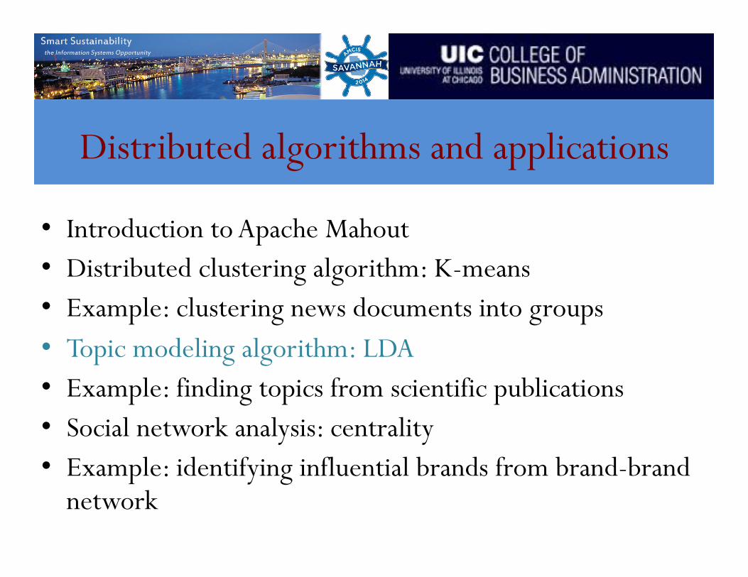
Distributed algorithms and applications

•  Introduction to Apache Mahout •  Distributed clustering algorithm: K-means •  Example: clustering news documents into groups •  Topic modeling algorithm: LDA •  Example: finding topics from job postings •  Social network analysis: centrality •  Example: identifying influential brands from brand-brand

network

Apache Mahout

•  Apache mahout(https://mahout.apache.org/) is an open-source scalable machine learning library. Many supervised and unsupervised algorithms are implemented and included.

•  List of algorithms – Collaborative filtering (mapreduce based) •  Item-based collaborative filtering •  Matrix factorization

List of algorithms – mapreduce based

•  Classification –  Naïve bayes –  Random forest

•  Clustering –  K-means / fuzzy K-means –  Spectral clustering

•  Dimensionality reduction –  Stochastic singular value decomposition –  Principle component analysis (PCA)

•  Topic modeling –  Latent dirichlet allocation (LDA)

•  And others –  Frequent itemset mining

Install Mahout

•  I suggest to download the stable version 0.7 mahout-distribution-0.7.tar.gz from http://archive.apache.org/dist/mahout/0.7/

•  Unpack and put it into a folder of your choice.



network

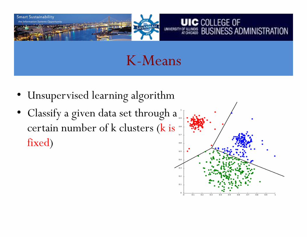
K-Means

•  Unsupervised learning algorithm •  Classify a given data set through a

certain number of k clusters (k is fixed)

Description

•  Given a set of observations (x1, x2, …, xn), where each observation is a d-dimensional real vector, k-means clustering aims to partition the n observations into k sets (k ≤ n): S = {S1, S2, …, Sk}, so as to minimize the within-cluster sum of squares (WCSS):

where μi is the mean of points in Si.

Algorithm

1.  Place K points into the space represented by the objects that are being clustered. These points represent initial group centroids.

2.  Assign each object to the group that has the closest centroid. 3.  When all objects have been assigned, recalculate the positions

of the K centroids. 4.  Repeat Steps 2 and 3 until the centroids no longer move. This

produces a separation of the objects into groups from which the metric to be minimized can be calculated.

Demonstration

k initial "means" (in this case k=3) are randomly generated within the data domain (shown in color).

k clusters are created by associating every observation with the nearest mean. The partitions here represent the Voronoi diagram generated by the means.

The centroid of each of the k clusters becomes the new mean.

Steps 2 and 3 are repeated until convergence has been reached.

Interpretation in math

•  Given an initial set of k means m1(1),…,mk

(1), the algorithm proceeds by alternating between two steps:

•  Assignment step: Assign each observation to the cluster whose mean yields the least within-cluster sum of squares (WCSS). Since the sum of squares is the squared Euclidean distance, this is intuitively the "nearest" mean.(Mathematically, this means partitioning the observations according to the Voronoi diagram generated by the means).

where each xp is assigned to exactly one S(t), even if it could be is assigned to two or more of them.

•  Update step: Calculate the new means to be the centroids of the observations in the new clusters.

Since the arithmetic mean is a least-squares estimator, this also minimizes the within-cluster sum of squares (WCSS) objective.

•  The algorithm has converged when the assignments no longer change.

Remarks

•  The way to initialize the means was not specified. One popular way to start is to randomly choose k of the samples.

•  The results produced depend on the initial values for the means, and it frequently happens that suboptimal partitions are found. The standard solution is to try a number of different starting points.

•  It can happen that the set of samples closest to mi is empty, so that mi cannot be updated. This is an annoyance that must be handled in an implementation, but that we shall ignore.

•  The results depend on the metric used to measure || x - mi ||. A popular solution is to normalize each variable by its standard deviation, though this is not always desirable.

•  The results depend on the value of k.

K-Means under MapReduce

•  Iterative MapReduce framework •  The implementation accepts two input directories – Data points

•  The data directory contains multiple input files of SequenceFile(key, VectorWritable),

–  The initial clusters •  The clusters directory contains one or more SequenceFiles(Text, Cluster |

Canopy) containing k initial clusters or canopies.

•  None of the input directories are modified by the implementation, allowing experimentation with initial clustering and convergence values.

Mapper class

•  Reads the input clusters during its setup() method, then assigns and outputs each input point to its nearest cluster as defined by the user-supplied distance measure. – Output key: Cluster Identifier. – Output value: Cluster Observation.

After mapper

•  Data {1.0, 1.0} à C1, {1.0, 1.0} {1.0, 3.0} à C1, {1.0, 3.0} {3.0, 1.0} à C2, {3.0, 1.0} {3.0, 3.0} à C2, {3.0, 3.0} {8.0, 8.0} à C2, {8.0, 8.0}

•  Cluster centroids (K=2) C1: {1.0, 1.0} C2: {3.0, 3.0}

Combiner class

•  Receives all (key : value) pairs from the mapper and produces partial sums of the input vectors for each cluster. – Output key is: Cluster Identifier. – Output value is: Cluster Observation.

After combiner

•  Data {1.0, 1.0} à C1, {1.0, 1.0} {1.0, 3.0} à C1, {1.0, 3.0} {3.0, 1.0} à C2, {3.0, 1.0} {3.0, 3.0} à C2, {3.0, 3.0} {8.0, 8.0} à C2, {8.0, 8.0}

•  Cluster centroids (K=2) C1: {1.0, 1.0} C2: {3.0, 3.0}

C1, {{1.0, 1.0},{1.0, 3.0}}

C2, {{3.0, 1.0},{3.0, 3.0}}

C2, {{8.0, 8.0}}

Reducer class

•  A single reducer receives all (key : value) pairs from all combiners and sums them to produce a new centroid for the cluster which is output. – Output key is: encoded cluster identifier. – Output value is: Cluster.

•  The reducer encodes un-converged clusters with a 'Cn' cluster Id and converged clusters with 'Vn' cluster Id.

After reducer

•  Data {1.0, 1.0} à C1, {1.0, 1.0} {1.0, 3.0} à C1, {1.0, 3.0} {3.0, 1.0} à C2, {3.0, 1.0} {3.0, 3.0} à C2, {3.0, 3.0} {8.0, 8.0} à C2, {8.0, 8.0}

•  Cluster centroids (K=2) C1: {1.0, 1.0} à Cn1: {1.0, 2.0} C2: {3.0, 3.0} à Cn2: {5.5, 5.0}

C1, {{1.0, 1.0},{1.0, 3.0}}

C2, {{3.0, 1.0},{3.0, 3.0}}

C2, {{8.0, 8.0}}

Driver class

•  Iterates over the points and clusters until –  all output clusters have converged (Vn clusterIds) –  or a maximum number of iterations has been reached.

•  During iterations, a new cluster directory "clusters-N" is produced with the output clusters from the previous iteration used for input to the next.

•  A final optional pass over the data using the KMeansClusterMapper clusters all points to an output directory "clusteredPoints" and has no combiner or reducer steps.

After multiple iterations

•  Data – {1.0, 1.0} à C1, {1.0, 1.0} …à C1, {2.0, 2.0} – {1.0, 3.0} à C1, {1.0, 3.0} …à C1, {2.0, 2.0} – {3.0, 1.0} à C2, {3.0, 1.0} …à C1, {2.0, 2.0} – {3.0, 3.0} à C2, {3.0, 3.0} …à C1, {2.0, 2.0} – {8.0, 8.0} à C2, {8.0, 8.0} …à C2, {8.0, 8.0}

•  Cluster centroids (K=2) – C1: {1.0, 1.0} …à Vn1: {2.0, 2.0} – C2: {3.0, 3.0} …à Vn2: {8.0, 8.0}

Running K-Means under mahout

$./bin/mahout kmeans -i <input vectors directory> -c <input clusters directory> -o <output working directory> -k <optional number of initial clusters to sample from input vectors> -dm <DistanceMeasure> -x <maximum number of iterations> -cd <optional convergence delta. Default is 0.5> -ow <overwrite output directory if present> -cl <run input vector clustering after computing Canopies> -xm <execution method: sequential or mapreduce>



network

Example:clustering news documents into groups

Check the Mahout_Kmeans document


•  Introduction to Apache Mahout •  Distributed clustering algorithm: K-means •  Example: clustering news documents into groups •  Topic modeling algorithm: LDA •  Example: finding topics from scientific publications •  Social network analysis: centrality •  Example: identifying influential brands from brand-brand

network

Topic modeling algorithm: LDA

•  Data as arising from a (imaginary) generative process –  probabilistic process that includes hidden variables

(latent topic structure)

•  Infer this hidden topic structure –  learn the conditional distribution of hidden variables, given the

observed data (documents)

Generative process for each document –  choose a distribution over topics –  for each word

draw a topic from the chosen topic distribution draw a word from distribution of words in the topic


D Nd K

βk

topics

Zd,n

topic assignment for word

Wd,n

observed word

θd

topic proportions for document

α V-dimensional Dirichlet

η K-dimensional Dirichlet

Joint distribution


Need to compute the posterior distribution

Intractable to compute exactly, approximation methods used - Variational inference (VEM) - Sampling (Gibbs)

David Blei, A. Ng, M. I. Jordan, Michael I. "Latent Dirichlet allocation”. Journal of Machine Learning Research, 2003.

David Blei. “Probabilistic topic models”. Communications of the ACM, 2012.

Example: finding topics job postings


network

Data

•  “Aggregates job listings from thousands of websites, including job boards, newspapers, associations, and company career pages….Indeed is currently available in 53 countries. In 2010, Indeed surpassed monster.com to become the most visited job site in the US. Currently Indeed has 60 million unique visitors every month.” (Wikipedia)

Social media jobs

Gross state product

Population

Social media jobs

Manufacturing

Consulting services

Information

Education Services

Other Services (except Public Administration) Health Care and Social

Assistance

Finance and Insurance

Administrative and Services, Retail Trade

Marketing and Advertising services

Transportation and Warehousing

Wholesale Trade

Arts, Entertainment, and Recreation

Construction

Real Estate and Rental and Leasing

Public Administration

Accommodation and Food Services

Legal Services

Design Services

Utilities Engineering Services Agriculture, Forestry, Fishing and Hunting

Management of Companies and

Enterprises

Mining Jobs by industry

Topic models in job ads

digital .23 creative .18 advertising. 16 brand .09 …

community .2 engage .18 editor .13 content .09 …

data .27 analytics .18 Intelligence .12 Insight .11 …

develop .31 code .22 agile .08 java .03 …

video .27 entertain .21 film .17 artist .04 virtual

Community: 0.76 Content: 0.13 Marketing: .071

Technology : 0.31 Leadership: 0.23 Strategy: 0.18

Marketing : 0.41 Analytics: 0.28 Campaign: 0.20

Jobs: distribution over topics

Topics (distribution over terms)

Topic models in job ads

•  Vocabulary –  filter out commonly used

terms, and very rare terms stemming

•  How many topics? –  ‘Perplexity’ measure on test data with varying

#-topics Cross-validation on 3000 job-ads

•  Interpretability –  Fewer topics: broader themes –  Too many topics: overly specific, non-

distinguished topics spurious term associations

800

820

840

860

880

900

920

940

960

30 40 50 60 70 80 90

perp

lexi

ty

# topics

Topics in job ads

(topic model with 50 topics) •  Topics pertaining to –  marketing, advertising, campaigns, brand management –  content management, graphic design –  community engagement, communication, coordinate/relationship,

customer service –  software development, enterprise technology, coding –  data /analytics, search optimization –  administrative assistance, consulting, innovation & leadership, strategy –  education, healthcare, entertainment, global –  benefits, abilities & qualification –  ….

Topic examples

Campaign Campaign, twitter, blog, social media, marketing campaign, linkedin, campaign management, email campaign, flickr, youtube, pineterest, advertising campaign,

Technical, software software, engineer, cloud, service, software development, server, data, infrastructure, technical, device, hardware, cloud computing, computer science, engineering team

Strategy leadership

Strategy, leadership, manage, leader, collaborate, engage, strategic plan, partnership, stakeholder, budget, achieve, vision, coach, complex, thought-leadership

Data, Analytics

Data, analytics, analyze, research, intelligence, recommend, insight, quantitative, statistical, business intelligence, analytical skill, evaluate, database, analytical tool

Education Student, education, college, campus, academic, faculty, service, undergraduate, collaborate, culture, dean, ambassador, administrative, assess, supervise

Product management

Product, define, product mgt, experience, translate, stakeholder, definition, vision, cross functional, development process, communicate, user experience, agile

Marketing Marketing, promotion, product, strategy, advertising, social, marketing communication, marketing strategy, social media, communicate, research, market relation

Social media focused

Social media, twitter, blog, platform, engage, linkedin, social network, communicate, manage social, strategy, facebook, creative, channel, social marketing, develop social

Jobs by topics

Marketing-related

Design/development

Manage –relationship /partner /

coordinate /promote Project management

Customer service, support

Strategy, leadership

Administrative assistance

Product-development /management

Communication

Content management

Community, fundraising

Education

Analytics Consulting



network

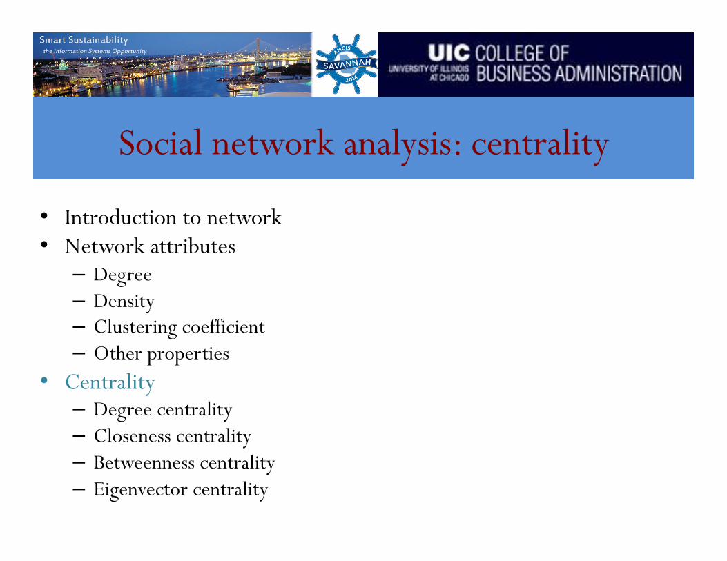
Social network analysis: centrality

•  Introduction to network •  Network attributes –  Degree –  Density –  Clustering coefficient –  Other properties

•  Centrality –  Degree centrality –  Closeness centrality –  Betweenness centrality –  Eigenvector centrality

Interesting networks

Patent citation network



Political blog network


Airport network

Network representation (I)

•  The adjacency matrix – Aij = 1 if node i and j are

connected, 0 otherwise for undirected network

– Aij = 1 if node j connects to i, 0 otherwise for directed network

– Aij = Wij for weighted network

Network representation (II)

•  The link table – Adjacency matrix needs

more computer memories – Each line would be (node i, node j, weight) for weighted network and (node i, node j) for unweighted network

1  2 1 3 2 1 2  4 3  1 3 4 4 2 4 3 4 5 5 4 5 6 6 5




Degree

•  The degree of a node i represents how many connections to its neighbors for unweighted network and reflects how strong connects to its neighbors for weighted network.

•  It can be computed from the adjacency matrix A. •  Average node degree of the entire network

ki = Ajij∑

< k >= 1N

kii∑ =

Aijij∑

N

Density

•  The ratio of links L and the maximum number of links which is N(N-1)/2 for an undirected network

•  It is the mean degree per node or the fraction of links a node has on average normalized by the potential number of neighbors

ρ =2L

N(N −1)=< k >N −1

≅< k >N

Clustering coefficient

•  A measure of “all-my-friends-know-each-other” •  More precisely, the clustering coefficient of a node is the

ratio of existing links connecting a node's neighbors to each other to the maximum possible number of such links.

•  The clustering coefficient for the entire network is the average of the clustering coefficients of all the nodes.

•  A high clustering coefficient for a network is another indication of a small world.

Clustering coefficient

•  Where ki is the neighbors of the ith node, ei is the number of connections between these neighbors

Ci =2ei

ki (ki −1)

Other properties

•  Network diameter: the longest of all shortest paths in a network

•  Path: a finite or infinite sequence of edges which connect a sequence of vertices which, by most definitions, are all distinct from one another

•  Shortest path: a path between two vertices (or nodes) in a graph such that the sum of the weights of its constituent edges is minimized




Centrality in a network

•  Information about the relative importance of nodes and edges in a graph can be obtained through centrality measures

•  Centrality measures are essential when a network analysis has to answer the following questions – Which nodes in the network should be targeted to ensure that a

message or information spreads to all or most nodes in the network? – Which nodes should be targeted to curtail the spread of a disease? – Which node is the most influential node?

Degree centrality

•  The number of links incident upon a node •  The degree can be interpreted in terms of the immediate risk

of a node for catching whatever is flowing through the network (such as a virus, or some information)

•  In the case of a directed network, indegree is a count of the number of ties directed to the node and outdegree is the number of ties that the node directs to others

•  When ties are associated to some positive aspects such as friendship or collaboration, indegree is often interpreted as a form of popularity, and outdegree as gregariousness

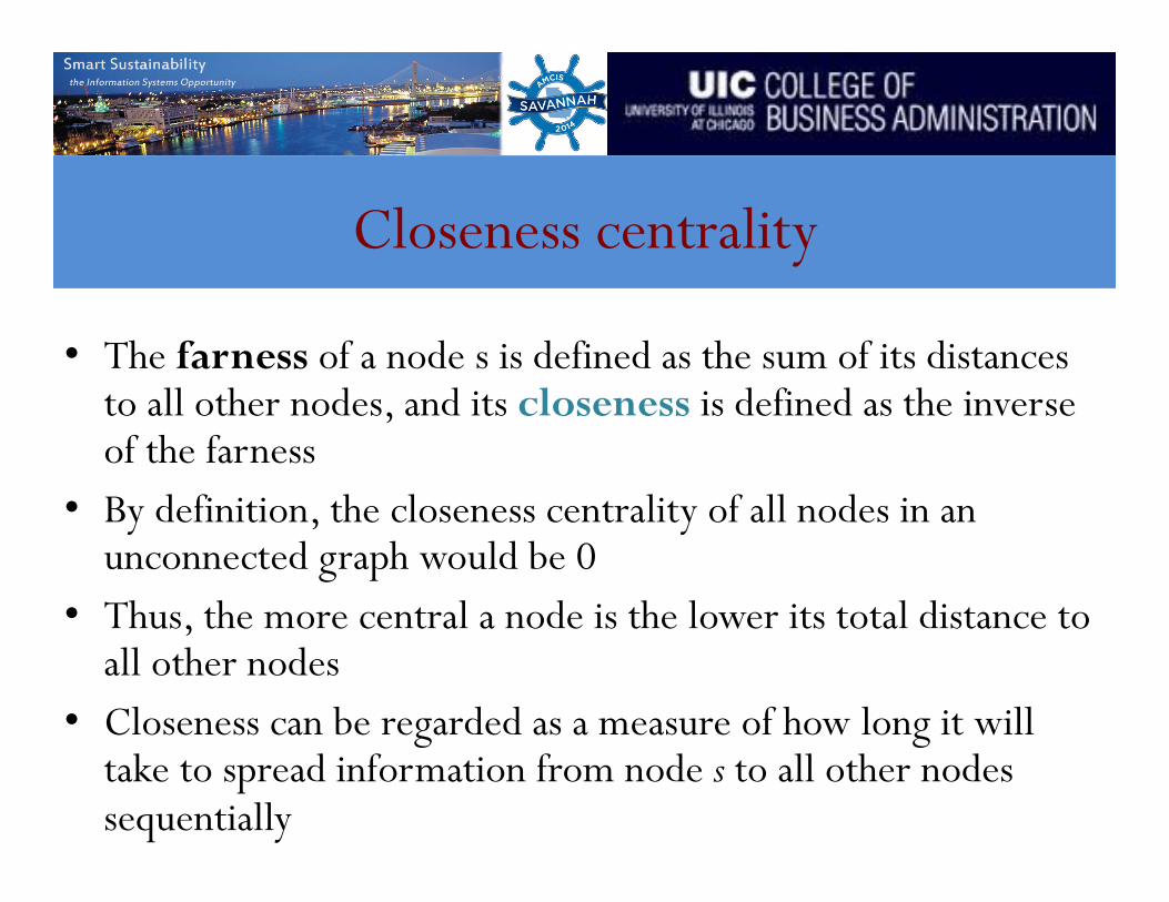
Closeness centrality

•  The farness of a node s is defined as the sum of its distances to all other nodes, and its closeness is defined as the inverse of the farness

•  By definition, the closeness centrality of all nodes in an unconnected graph would be 0

•  Thus, the more central a node is the lower its total distance to all other nodes

•  Closeness can be regarded as a measure of how long it will take to spread information from node s to all other nodes sequentially

Application

•  High closeness centrality individuals tend to be important influencers within their local network community. They may often not be public figures to the entire network of a corporation or profession, but they are often respected locally and they occupy short paths for information spread within their network community

Betweenness centrality

•  It quantifies the number of times a node acts as a bridge along the shortest path between two other nodes

•  The betweenness of a vertex v in a graph G:=(V, E) with V vertices is computed as follows: 1.  For each pair of vertices (s, t), compute the shortest paths

between them. 2.  For each pair of vertices (s, t), determine the fraction of

shortest paths that pass through the vertex in question (here, vertex v).

3.  Sum this fraction over all pairs of vertices (s, t).

Betweenness centrality

•  Where is the total number of shortest paths from node s to node t and is the number of those paths that pass through v.

CB (v) =σ st (v)σ sts≠v≠t∉V

∑

σ st

σ st (v)

Application

•  High betweenness individuals are often critical to collaboration across departments and to maintaining the spread of a new product through an entire network. Because of their locations between network communities, they are natural brokers of information and collaboration.

Eigenvector centrality

•  A measure of the influence of a node in a network •  It assigns relative scores to all nodes in the network based

on the concept that connections to high-scoring nodes contribute more to the score of the node in question than equal connections to low-scoring nodes

•  Google's PageRank is a variant of the eigenvector centrality measure

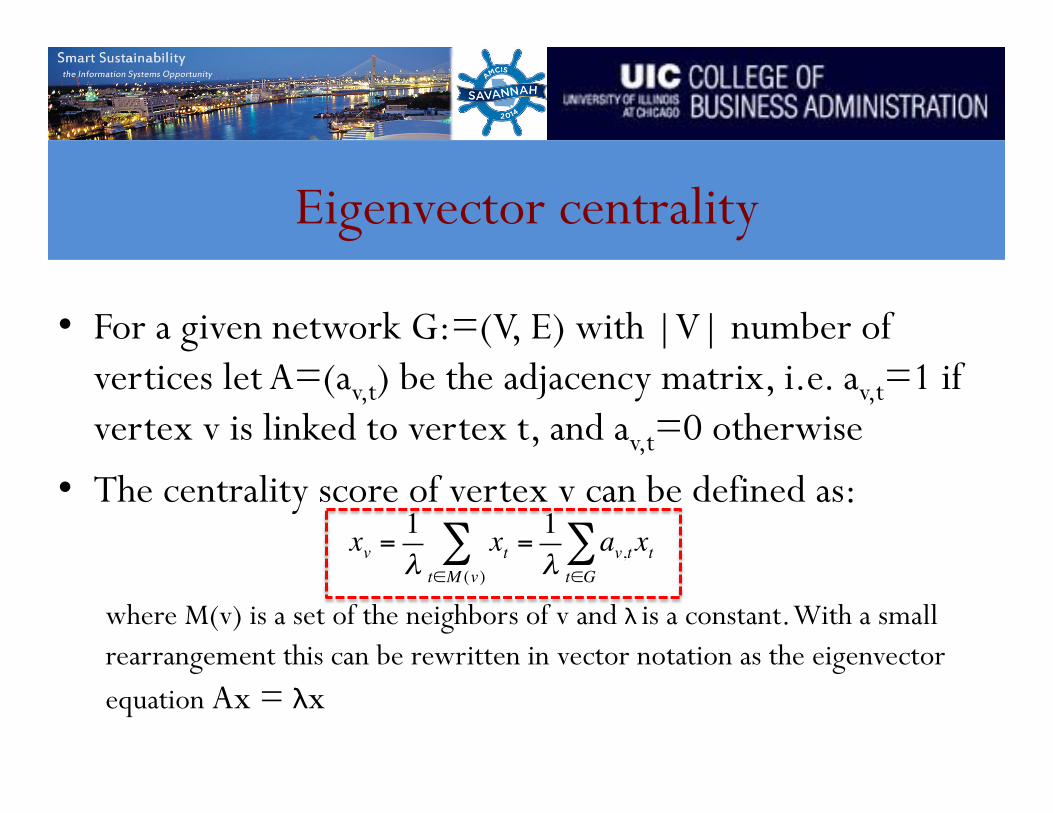
Eigenvector centrality

•  For a given network G:=(V, E) with |V| number of vertices let A=(av,t) be the adjacency matrix, i.e. av,t=1 if vertex v is linked to vertex t, and av,t=0 otherwise

•  The centrality score of vertex v can be defined as:

where M(v) is a set of the neighbors of v and λ is a constant. With a small rearrangement this can be rewritten in vector notation as the eigenvector equation Ax = λx

xv =1λ

xtt∈M (v)∑ =

1λ

av,t xtt∈G∑

Application

•  High eigenvector centrality individuals are leaders of the network. They are often public figures with many connections to other high-profile individuals. Thus, they often play roles of key opinion leaders and shape public perception. High eigenvector centrality individuals, however, cannot necessarily perform the roles of high closeness and betweenness. They do not always have the greatest local influence and may have limited brokering potential.

Real data example

•  Undirected and weighted brand-brand network from Facebook – Nodes: social brands (e.g., institutions, organizations,

universities, celebrities, etc.) – Links: if two brands have common users who had activities

(liked, made comments) on both brands – Weights: the number of common users (normalized)

•  2000 brands are selected based on their sizes

Distribution of eigenvector centrality

10 most and least influential brands

Schedule


V. Conclusion

Conclusion

•  What is big data? •  Why big matters to you? •  What are techniques for big data analytics? •  Hadoop and MapReduce •  Clustering algorithm: K-means •  Topic modeling algorithm: LDA •  Social network analysis: centrality

What is big data?

•  Five Vs – Volume: the size of data – Velocity: the change speed of data, streaming generating data – Variety: the format of data is various – Veracity: the truth of data – Value: companies can benefit from big data analysis

Why big data matters to you?

•  Big data analytics has been occurred in every domain, including finance, government, science, healthcare, IT, etc.

•  Big data becomes a hot word in job descriptions •  Many companies benefit from big data analysis

Techniques in big data analytics

•  Machine learning •  Text/web mining •  Distributed computing •  Social network analysis •  Natural language processing •  Visualization •  Optimization


•  Hadoop is a platform

•  MapReduce is a computing mechanism

HDFS architecture

MapReduce framework

•  Per cluster node: – Single JobTracker per master •  Responsible for scheduling the

jobs’ component tasks on the slaves •  Monitor slave progress •  Re-execute failed tasks

– Single TaskTracker per slave •  Execute the task as directed by

the master

Hadoop data flow

K-Means

k initial "means" (in this case k=3) are randomly generated within the data domain (shown in color).

k clusters are created by associating every observation with the nearest mean. The partitions here represent the Voronoi diagram generated by the means.

The centroid of each of the k clusters becomes the new mean.

Steps 2 and 3 are repeated until convergence has been reached.


D Nd K

βk

topics

Zd,n

topic assignment for word

Wd,n

observed word

θd

topic proportions for document

α V-dimensional Dirichlet

η K-dimensional Dirichlet

Joint distribution

Network analysis: centrality

•  Degree centrality of a node in a network is the number of links (vertices) incident on the node.

•  Closeness centrality determines how “close” a node is to other nodes in a network by measuring the sum of the shortest distances (geodesic paths) between that node and all other nodes in the network.

•  Betweenness centrality determines the relative importance of a node by measuring the amount of traffic flowing through that node to other nodes in the network. This is done by measuring the fraction of paths connecting all pairs of nodes and containing the node of interest.

•  Eigenvector centrality is a more sophisticated version of degree centrality where the centrality of a node not only depends on the number of links incident on the node but also the quality of those links. This quality factor is determined by the eigenvectors of the adjacency matrix of the network.

Some tools (I)

•  Weka 3: data mining software in Java http://www.cs.waikato.ac.nz/ml/weka/

•  Apache Mahout: scalable machine learning library https://mahout.apache.org/

•  Natural language toolkit (NLTK) http://www.nltk.org/ •  Gephi: network analysis http://gephi.github.io/

Some tools (II)

•  igraph: network analysis package http://igraph.org/redirect.html

•  Data visualization http://d3js.org/ •  Hive: distributed data warehouse

http://hive.apache.org/ •  Pig: analyzing large dataset

http://pig.apache.org/

Recommended papers

•  Big data report: http://www.mckinsey.com/insights/business_technology/big_data_the_next_frontier_for_innovation

•  MapReduce:

http://static.googleusercontent.com/media/research.google.com/en/us/archive/mapreduce-osdi04.pdf

Recommended papers

•  Machine learning algorithm survey: http://www.cs.umd.edu/~samir/498/10Algorithms-08.pdf

•  Community detection in a network survey: http://arxiv.org/abs/0906.0612

•  Topic modeling: https://www.cs.princeton.edu/~blei/papers/Blei2011.pdf

Thank you

Documents

Tutorial: Big Data Algorithms and Applications …kpzhang/tutorial/amcis2014_files/...Tutorial: Big Data Algorithms and Applications Under Hadoop KUNPENG ZHANG SIDDHARTHA BHATTACHARYYA