Embed Size (px)
Citation preview

1
2
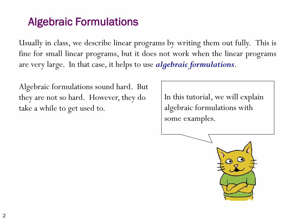
Algebraic Formulations
Usually in class, we describe linear programs by writing them out fully. This is fine for small linear programs, but it does not work when the linear programs are very large. In that case, it helps to use algebraic formulations.
Algebraic formulations sound hard. But they are not so hard. However, they do take a while to get used to.
In this tutorial, we will explain algebraic formulations with some examples. Algebraic
3
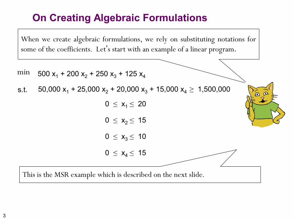
On Creating Algebraic Formulations
min 500 x1 + 200 x2 + 250 x3 + 125 x4
s.t. 50,000 x1 + 25,000 x2 + 20,000 x3 + 15,000 x4 ≥ 1,500,000
0 ≤ x1 ≤ 20
0 ≤ x2 ≤ 15
0 ≤ x3 ≤ 10
0 ≤ x4 ≤ 15
When we create algebraic formulations, we rely on substituting notations for some of the coefficients. Let’s start with an example of a linear program.
This is the MSR example which is described on the next slide.

4
MSR Marketing Inc. adapted from Frontline Systems
•Need to choose ads to reach at least 1.5 million people
•Minimize Cost
•Upper bound on number of ads of each type
TV
Radio
Newspaper
Audience Size
50,000
25,000
20,000
15,000
Cost/Impression
$500
$200
$250
$125
Max # of ads
20
15
10
15
Decision variables: • x1 is the number of TV ads. • x2 is the number of radio ads. • x3 is the number of mail ads. • x4 is the number of newspaper ads.
5
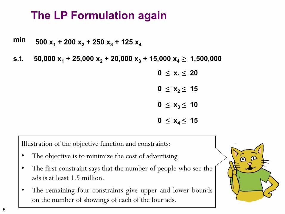
The LP Formulation again
min 500 x1 + 200 x2 + 250 x3 + 125 x4
s.t. 50,000 x1 + 25,000 x2 + 20,000 x3 + 15,000 x4 ≥ 1,500,000
0 ≤ x1 ≤ 20
0 ≤ x2 ≤ 15
0 ≤ x3 ≤ 10
0 ≤ x4 ≤ 15
Illustration of the objective function and constraints:
• The objective is to minimize the cost of advertising.
• The first constraint says that the number of people who see the ads is at least 1.5 million.
• The remaining four constraints give upper and lower bounds on the number of showings of each of the four ads.
6
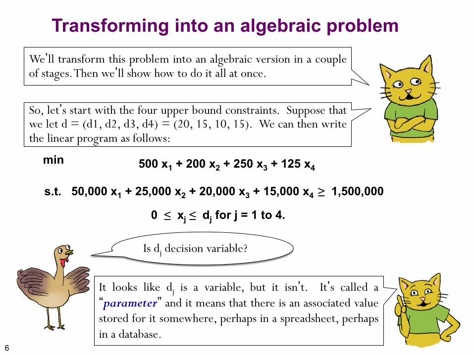
Transforming into an algebraic problem
min 500 x1 + 200 x2 + 250 x3 + 125 x4
s.t. 50,000 x1 + 25,000 x2 + 20,000 x3 + 15,000 x4 ≥ 1,500,000
0 ≤ x1 ≤ 20; 0 ≤ x2 ≤ 15; 0 ≤ x3 ≤ 10; 0 ≤ x4 ≤ 15 0 ≤ xj ≤ dj for j = 1 to 4.
We’ll transform this problem into an algebraic version in a couple of stages. Then we’ll show how to do it all at once.
So, let’s start with the four upper bound constraints. Suppose that we let d = (d1, d2, d3, d4) = (20, 15, 10, 15). We can then write the linear program as follows:
Is dj decision variable?
It looks like dj is a variable, but it isn’t. It’s called a “parameter” and it means that there is an associated value stored for it somewhere, perhaps in a spreadsheet, perhaps in a database.
7
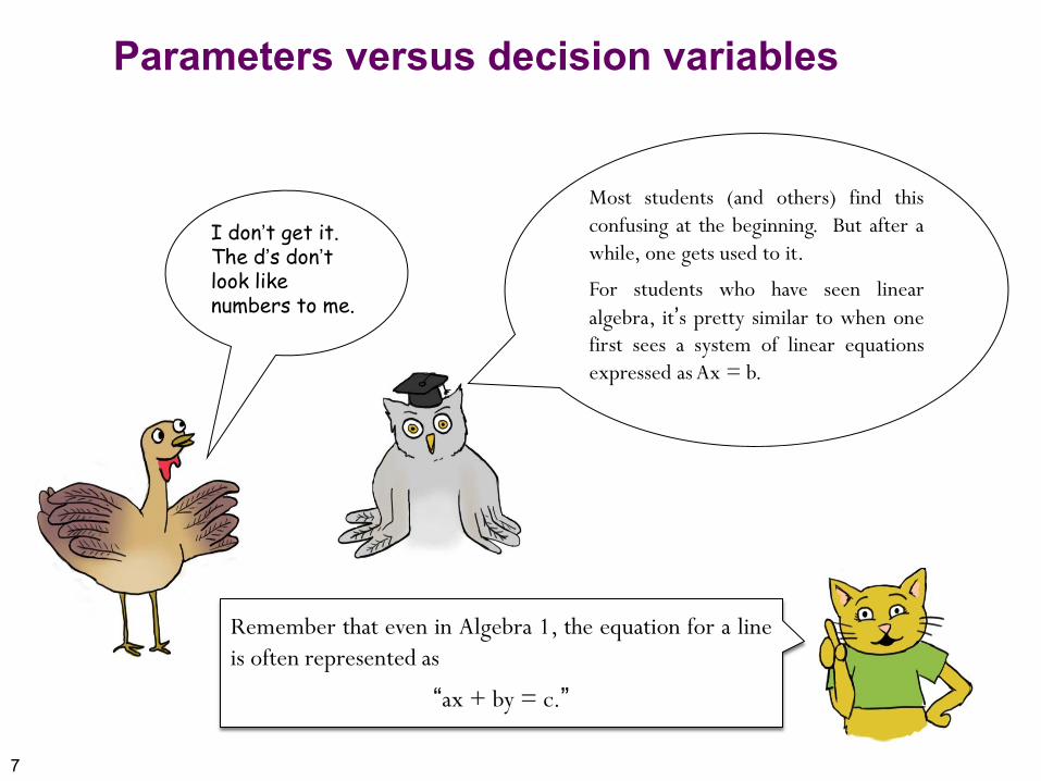
Parameters versus decision variables
I don’t get it. The d’s don’t look like numbers to me.
Most students (and others) find this confusing at the beginning. But after a while, one gets used to it.
For students who have seen linear algebra, it’s pretty similar to when one first sees a system of linear equations expressed as Ax = b.
Remember that even in Algebra 1, the equation for a line is often represented as
“ax + by = c.”
8
More on the algebraic formulation
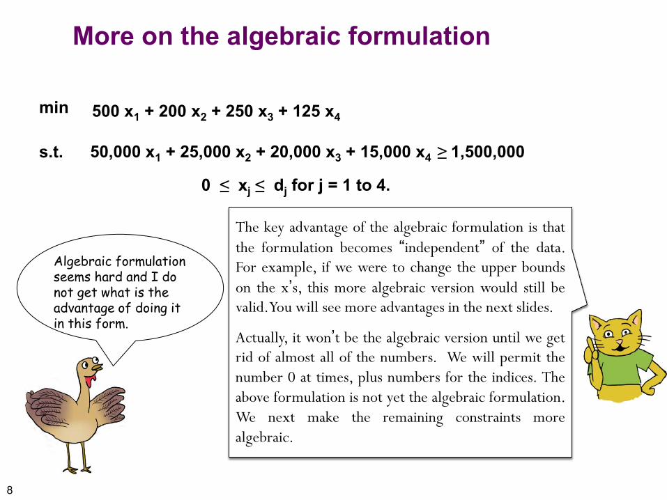
min 500 x1 + 200 x2 + 250 x3 + 125 x4
s.t. 50,000 x1 + 25,000 x2 + 20,000 x3 + 15,000 x4 ≥ 1,500,000
0 ≤ xj ≤ dj for j = 1 to 4.
The key advantage of the algebraic formulation is that the formulation becomes “independent” of the data. For example, if we were to change the upper bounds on the x’s, this more algebraic version would still be valid. You will see more advantages in the next slides.
Actually, it won’t be the algebraic version until we get rid of almost all of the numbers. We will permit the number 0 at times, plus numbers for the indices. The above formulation is not yet the algebraic formulation. We next make the remaining constraints more algebraic.
Algebraic formulation seems hard and I do not get what is the advantage of doing it in this form.
9
Making the remaining constraint more algebraic
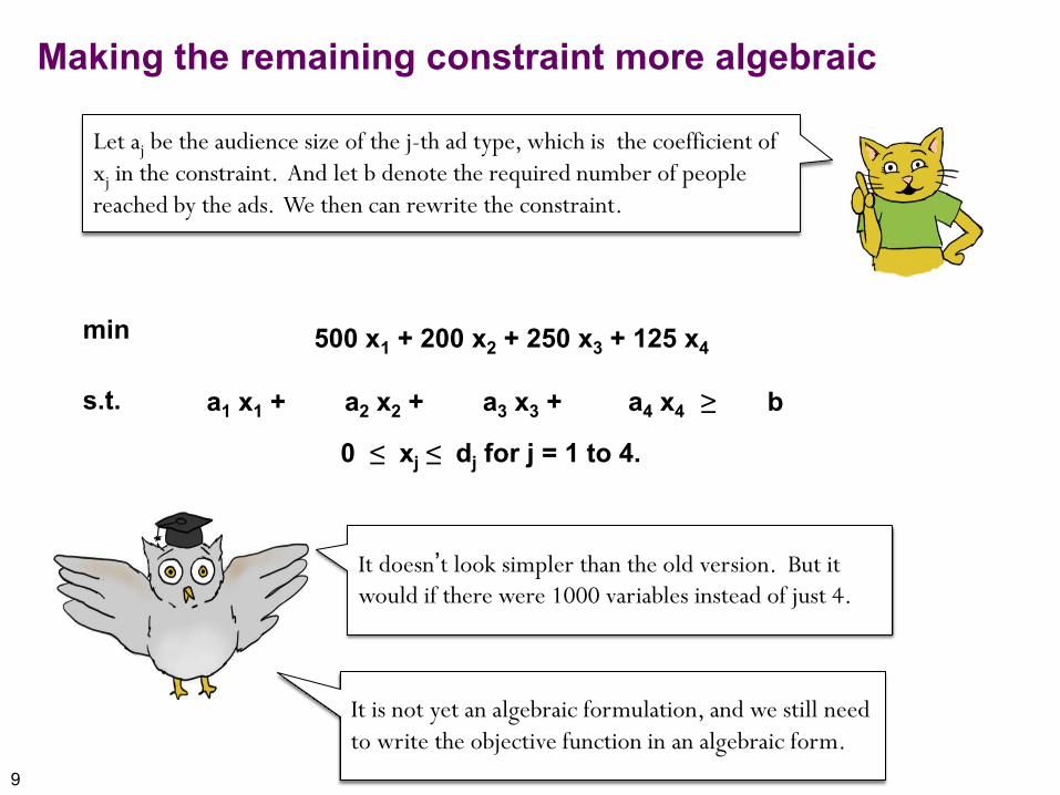
min 500 x1 + 200 x2 + 250 x3 + 125 x4
50,000 x1 + 25,000 x2 + 20,000 x3 + 15,000 x4 ≥ 1,500,000
0 ≤ xj ≤ dj for j = 1 to 4.
s.t. a1 x1 + a2 x2 + a3 x3 + a4 x4 ≥ b
Let aj be the audience size of the j-th ad type, which is the coefficient of xj in the constraint. And let b denote the required number of people reached by the ads. We then can rewrite the constraint.
It doesn’t look simpler than the old version. But it would if there were 1000 variables instead of just 4.
It is not yet an algebraic formulation, and we still need to write the objective function in an algebraic form.
10
Transforming the cost coefficients
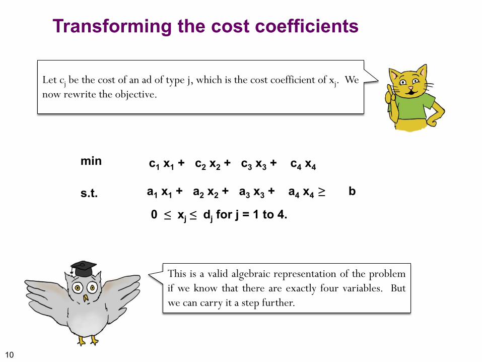
min 500 x1 + 200 x2 + 250 x3 + 125 x4
0 ≤ xj ≤ dj for j = 1 to 4.
s.t. a1 x1 + a2 x2 + a3 x3 + a4 x4 ≥ b
c1 x1 + c2 x2 + c3 x3 + c4 x4
Let cj be the cost of an ad of type j, which is the cost coefficient of xj. We now rewrite the objective.
This is a valid algebraic representation of the problem if we know that there are exactly four variables. But we can carry it a step further.
11
Using Summation Notation
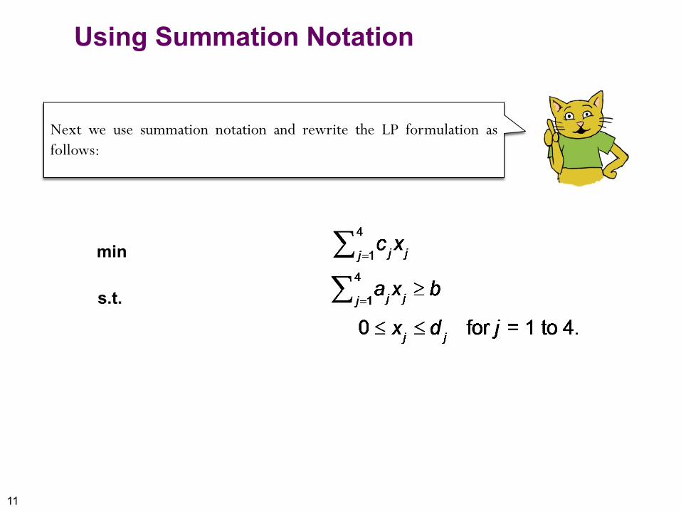
min
0 ≤ xj ≤ dj for j = 1 to 4.
s.t. a1 x1 + a2 x2 + a3 x3 + a4 x4 ≥ b
c1 x1 + c2 x2 + c3 x3 + c4 x4
Next we use summation notation and rewrite the LP formulation as follows:
12
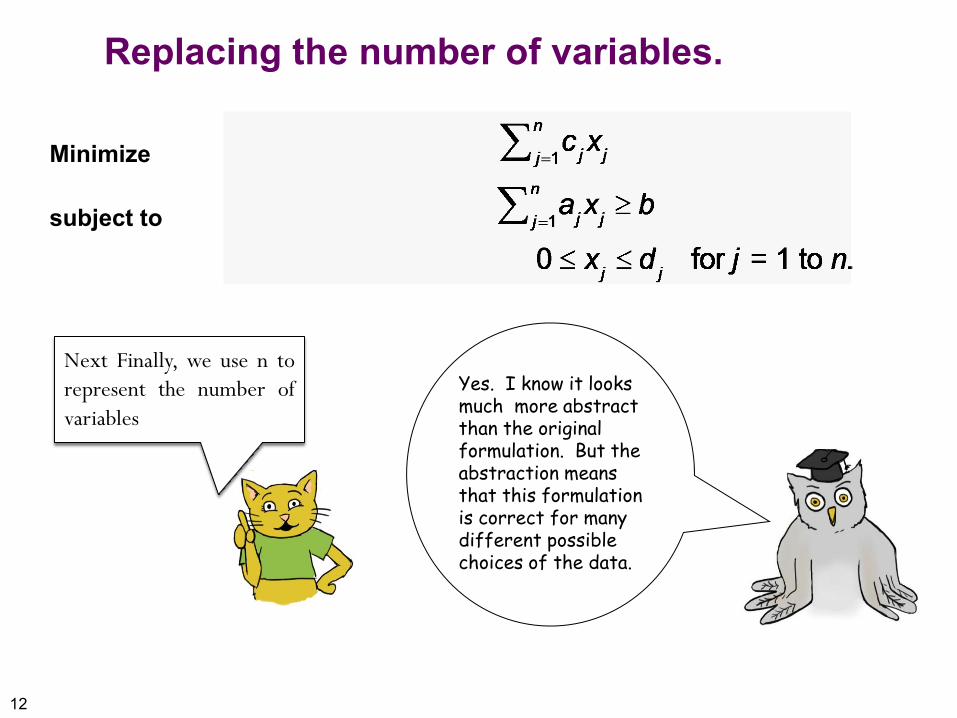
Replacing the number of variables.
Minimize
subject to
Yes. I know it looks much more abstract than the original formulation. But the abstraction means that this formulation is correct for many different possible choices of the data.
Next Finally, we use n to represent the number of variables.

13
Summary of the transformation
Minimize
subject to
Minimize 500 x1 + 200 x2 + 250 x3 + 125 x4
subject to 50,000 x1 + 25,000 x2 + 20,000 x3 + 15,000 x4 ≥ 1,500,000
0 ≤ x1 ≤ 20; 0 ≤ x2 ≤ 15; 0 ≤ x3 ≤ 10; 0 ≤ x4 ≤ 15;
• Let xj be the number of ads purchased of type j for j = 1 to n. • Let aj be the number of persons who view one ad of type j • Let b be the required number of viewers to see the ads. (That is, the total number of
viewers must be at least b) • Let dj be an upper bound on the number of ads purchased of type j.
14
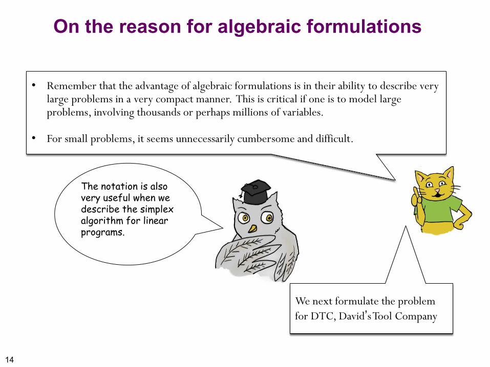
On the reason for algebraic formulations
The notation is also very useful when we describe the simplex algorithm for linear programs.
• Remember that the advantage of algebraic formulations is in their ability to describe very large problems in a very compact manner. This is critical if one is to model large problems, involving thousands or perhaps millions of variables.
• For small problems, it seems unnecessarily cumbersome and difficult.
We next formulate the problem for DTC, David’s Tool Company
15
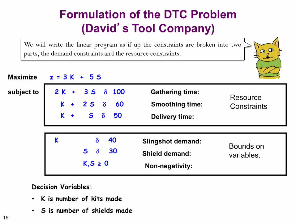
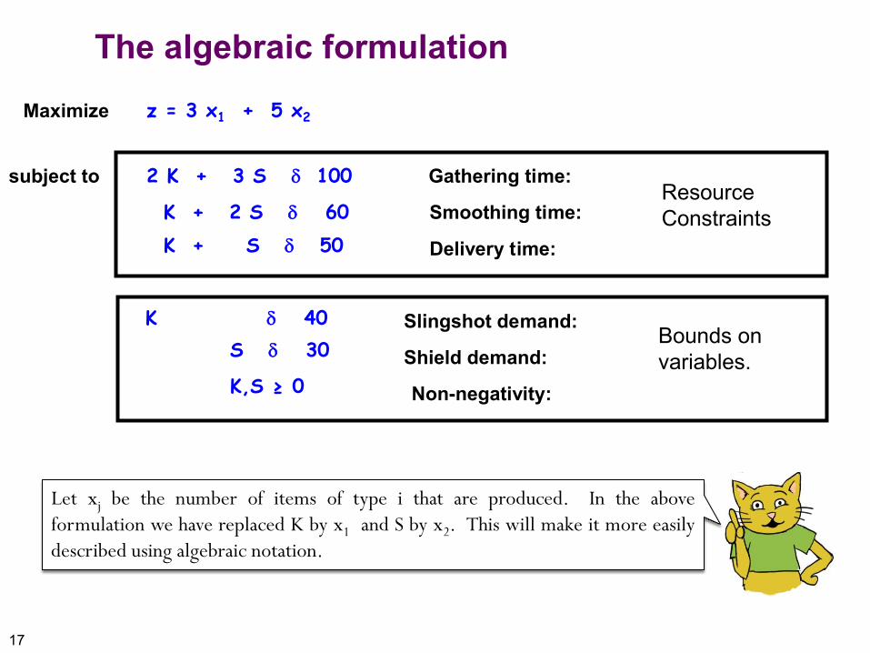
Formulation of the DTC Problem (David’s Tool Company)
z = 3 K + 5 S Maximize
2 K + 3 S δ 100
K + 2 S δ 60 K + S δ 50
Gathering time:
Smoothing time:
Delivery time:
subject to Resource Constraints
K,S ≥ 0
S δ 30 K δ 40
Shield demand:
Slingshot demand:
Non-negativity:
Bounds on variables.
Decision Variables:
• K is number of kits made
• S is number of shields made
We will write the linear program as if up the constraints are broken into two parts, the demand constraints and the resource constraints.
16
Before checking out the next page, try it for yourself. There are several correct answers. We will show one soon.
Don’t ask me. I have no clue what is going on. But I like watching others explain math.
17
z = 3 K + 5 S Maximize
The algebraic formulation z = 3 x1 + 5 x2
2 K + 3 S δ 100
K + 2 S δ 60 K + S δ 50
Gathering time:
Smoothing time:
Delivery time:
subject to Resource Constraints
K,S ≥ 0
S δ 30 K δ 40
Shield demand:
Slingshot demand:
Non-negativity:
Bounds on variables.
Let xj be the number of items of type i that are produced. In the above formulation we have replaced K by x1 and S by x2. This will make it more easily described using algebraic notation.
18
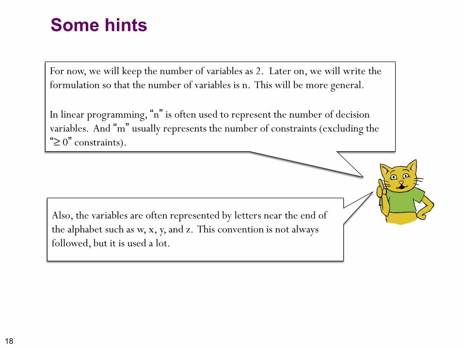
For now, we will keep the number of variables as 2. Later on, we will write the formulation so that the number of variables is n. This will be more general.
In linear programming, “n” is often used to represent the number of decision variables. And “m” usually represents the number of constraints (excluding the “≥ 0” constraints).
Also, the variables are often represented by letters near the end of the alphabet such as w, x, y, and z. This convention is not always followed, but it is used a lot.
Some hints
19
Resource Constraints
2 K + 3 S δ 100
K + 2 S δ 60 K + S δ 50
Gathering time:
Smoothing time:
Delivery time:
subject to Resource Constraints
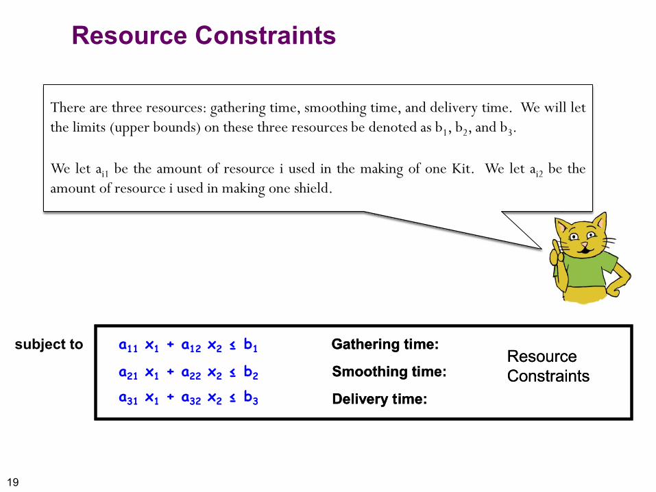
a11 x1 + a12 x2 ≤ b1
a21 x1 + a22 x2 ≤ b2
a31 x1 + a32 x2 ≤ b3
Gathering time:
Smoothing time:
Delivery time:
Resource Constraints
There are three resources: gathering time, smoothing time, and delivery time. We will let the limits (upper bounds) on these three resources be denoted as b1, b2, and b3. We let ai1 be the amount of resource i used in the making of one Kit. We let ai2 be the amount of resource i used in making one shield.
20
Resource Constraints
a11 x1 + a12 x2 ≤ b1
a21 x1 + a22 x2 ≤ b2
a31 x1 + a32 x2 ≤ b3
Gathering time:
Smoothing time:
Delivery time:
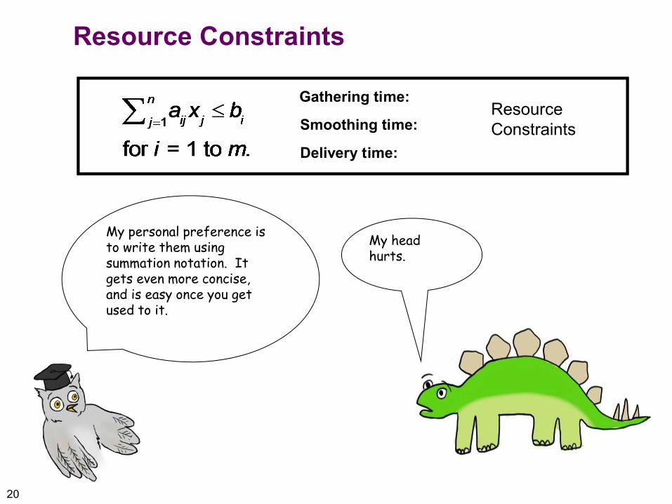
Resource Constraints
My personal preference is to write them using summation notation. It gets even more concise, and is easy once you get used to it.
Gathering time:
Smoothing time:
Delivery time:
Resource Constraints
My head hurts.

21
z = 3 x1 + 5 x2 Maximize
2 x1 + 3 x2 ≤ 100
x1 + 2 x2 ≤ 60 x1 + x2 ≤ 50
Gathering time:
Smoothing time:
Delivery time:
subject to Resource Constraints
x1, x2 ≥ 0
x2 ≤ 30 x1 ≤ 40
Shield demand:
Slingshot demand:
Non-negativity:
Bounds on variables.
The complete algebraic formulation
In this formulation:
dj : an upper bound on the demand for item j. n : the number of items. aij : the amount of resource i used up by one unit of item j.
m : the number of different resources. pj : the profit from making one unit of item j
Shield demand:
Slingshot demand:
Non-negativity:
Bounds on variables.
0 ≤ xj ≤ dj for j = 1 to n.
Gathering time:
Smoothing time:
Delivery time:
Resource Constraints
22
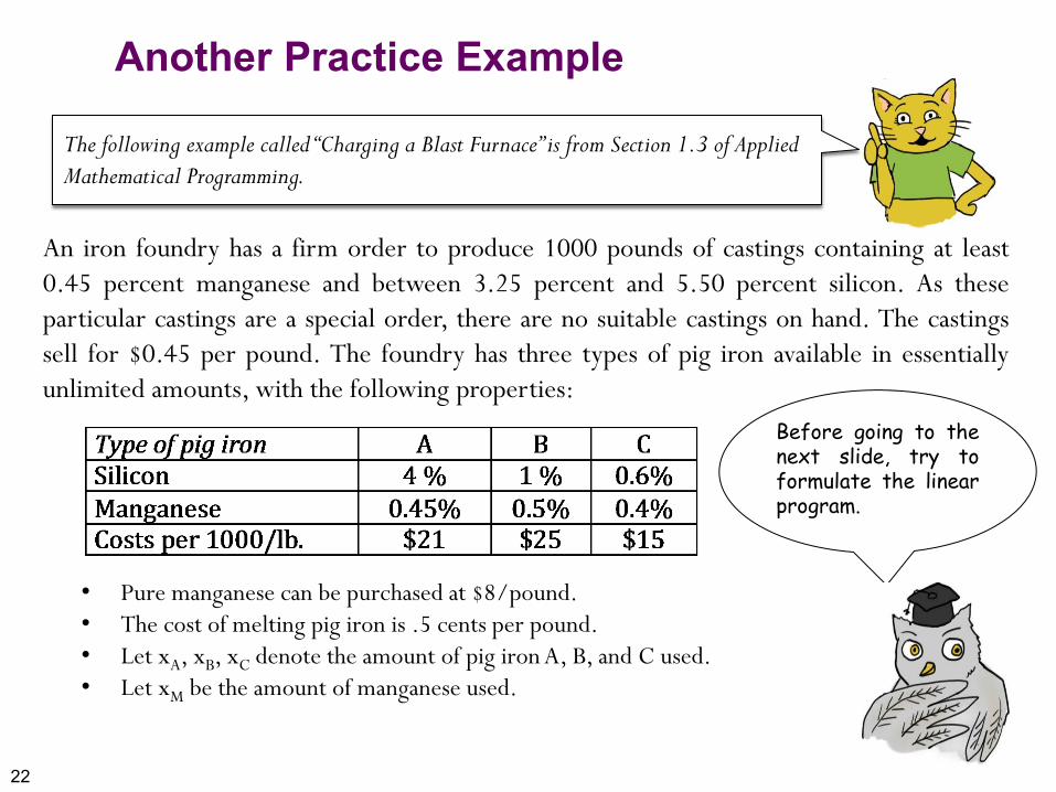
Another Practice Example
An iron foundry has a firm order to produce 1000 pounds of castings containing at least 0.45 percent manganese and between 3.25 percent and 5.50 percent silicon. As these particular castings are a special order, there are no suitable castings on hand. The castings sell for $0.45 per pound. The foundry has three types of pig iron available in essentially unlimited amounts, with the following properties:
• Pure manganese can be purchased at $8/pound. • The cost of melting pig iron is .5 cents per pound. • Let xA, xB, xC denote the amount of pig iron A, B, and C used. • Let xM be the amount of manganese used.
The following example called “Charging a Blast Furnace” is from Section 1.3 of Applied Mathematical Programming.
Before going to the next slide, try to formulate the linear program.

23
The LP formulation
maximize profit = revenue minus cost = 450 − 26xA − 30xB − 20xC − 8xM.
s.t. The mixture weighs 1000 pounds. 1000xA + 1000xB + 1000xB + xM = 1000.
The mixture has at least 4.5 pounds of manganese. 4.5xA + 5.0xB + 4.0xC + xM ≥ 4.5.
The amount of silicon is between 32.5 and 55 pounds. 40xA + 10xB + 6xC ≤ 32.5 40xA + 10xB + 6xC ≥ 55 Each variable is nonnegative. xA ≥ ,0 xB ≥ 0, xC ≥ 0, xM ≥ 0
To see the model, just
keep on clicking.
Objective
Weight constraint
Manganese constraint
Silicon constraints
The constraints that must always be remembered
24
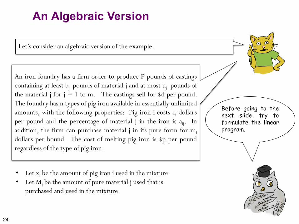
An Algebraic Version
• Let xi be the amount of pig iron i used in the mixture. • Let Mj be the amount of pure material j used that is
purchased and used in the mixture
Let’s consider an algebraic version of the example.
An iron foundry has a firm order to produce P pounds of castings containing at least bj pounds of material j and at most uj pounds of the material j for j = 1 to m. The castings sell for $d per pound. The foundry has n types of pig iron available in essentially unlimited amounts, with the following properties: Pig iron i costs ci dollars per pound and the percentage of material j in the iron is aij. In addition, the firm can purchase material j in its pure form for mi dollars per bound. The cost of melting pig iron is $p per pound regardless of the type of pig iron.
Before going to the next slide, try to formulate the linear program.

25
The LP formulation
maximize profit = Pd − Pp - ∑i ci xi - ∑j mj Mj
s.t. The mixture weighs P pounds. ∑i xi + ∑j Mj = P
The mixture has at least bj pounds of material j and at most uj pounds of material j. ∑i aij xi + ∑ Mj ≥ bj for j = 1 to m ∑i aij xi + ∑ Mj ≤ uj for j = 1 to m
Each variable is nonnegative. xi ≥ 0 for i = 1 to n Mj ≥ 0 for j = 1 to m
To see the model, just
keep on clicking.
Objective
Weight constraint
Material constraints
The constraints that must always be remembered
26
26
I hope that you are getting the hang of this now. If not, all it takes is some more practice.
If it helps, you can represent the notation so that it is easier to remember (but longer to write). We’ll do this on the next slide.
This is the manner in which it is usually described to a “modeling language”, which then rewrites the LP in a format that can be solved by a computer. We won’t be using modeling languages, but it is worth knowing that they exist.

27
27
SETS: IRONS: Set of pig irons MATERIALS: Set of materials VARIABLES: IronUsed(j): amount of iron i used, for j ∈ IRONS. Purchased(i) : = amount of material j purchased, for i ∈ MATERIALS PARAMETERS (Data) CastingRevenue: The price per pound for selling castings PigIronCost(j): Cost per pound of pig iron j for j ∈ IRONS MaterialCost(i): Cost per pound of material i for i ∈ MATERIALS MeltingCost = Cost per pound of melting any of the pig irons TotalCastings = number of pounds of castings to be sold Materials_Per_Iron(i, j) = The amount of material i in pig iron j for i ∈ MATERIALS and j ∈ IRONS. LowerLimit(i): The minimum fraction of Material i needed in the mixture UpperLimit(i): The maximum fraction of material i allowedin the mixture

28
LowerLimit(i) ≤ ∑j∈IRONS Materials_Per_Iron(i, j) × IronUsed(j) + ∑i∈MATERIALS Purchased(i) ≤ UpperLimit(i) for i ∈ Materials
The LP formulation, for the last time
28
max TotalCastings × CastingRevenue − ∑j∈IRONS [ MeltingCost(j) + PigIronCost(j)] IronUsed(j) − ∑i∈MATERIALS MaterialCost(i) × Purchased(i)
s.t. ∑j∈IRONS IronUsed(j) + ∑i∈MATERIALS Purchased(i) = TotalCastings
IronUsed(j) ≥ 0 for j ∈ IRONS Purchased(i) ≥ 0 for i ∈ MATERIALS
Objective
Weight constraint
Material constraints
The constraints that must always be remembered
29
29
The huge advantage of the previous formulation is that it is much easier to debug and extremely flexible. Notation is consistently used. Sets are well defined. Sets, Variables, and Parameters are all defined using easily understood terms. The presumption is that the data is all stored in a database that the “modeling language” can directly access.
If I don’t understand things in three different ways, am I doing better or worse?

30
Notation for linear programs in standard form
• Finally, we show some conventions that are used in describing a linear programming in standard form. The conventions are used in 15.053.
• There are usually n variables and m equality constraints • The variables are usually x1, …, xn. • The cost coefficients are usually c1, …, cn. (Objective function coefficients
are often called cost coefficients even if one is maximizing profit. It is widely agreed that this is a weird convention, but it is commonly done in any case.)
• The coefficient for xj in constraint i is aij. The RHS is bi. • Then the LP in “standard form” can be written as follows:
31
31
Last slide
In case you were wondering, there are different ways of writing algebraic formulations. You can choose notation differently, and you can combine groups of constraints differently.
You will have a chance to practice algebraic formulations on the homework sets. And that’s the end of this tutorial. I hope it was of value to you. Bye!
MIT OpenCourseWarehttp://ocw.mit.edu
15.053 Optimization Methods in Management ScienceSpring 2013
For information about citing these materials or our Terms of Use, visit: http://ocw.mit.edu/terms.