Embed Size (px)
Citation preview

UNIVERSITY OF CALIFORNIA
Los Angeles
The Development of Methods to Assess Radiation Dose to Organs
from Multidetector Computed Tomography Exams
Based on Detailed Monte Carlo Dosimetry Simulations
A dissertation submitted in partial satisfaction of the
requirements for the degree Doctor of Philosophy
in Biomedical Physics
by
Adam Christopher Turner
2011

© Copyright by
Adam Christopher Turner
2011

ii
The dissertation of Adam Christopher Turner is approved.
Christopher Cagnon
John DeMarco
Matthew Brown
David Saltzberg
Michael McNitt-Gray, Committee Chair
University of California, Los Angeles
2011

iii
I dedicate this dissertation to my parents Gary and Marilynn Turner.
I owe you everything.

iv
Table of Contents
Chapter 1 Background and Motivation ....................................................................................... 1
1.1 Radiation Risks from CT Exams ........................................................................................... 4
1.2 Routine Clinical CT Dosimetry Assessment (CTDI and DLP) ............................................. 6
1.3. Limitations of the CTDI ...................................................................................................... 10
1.4 Effective Dose from CT Exams and its Limitations ............................................................ 11
1.5. Existing Organ Dose Estimation Methods .......................................................................... 13
1.6. Discussion ........................................................................................................................... 18
Chapter 2 Specific Aims .............................................................................................................. 19
Chapter 3 UCLA Monte Carlo MDCT Dosimetry Package .................................................... 21
3.1 Radiation Transport Methods .............................................................................................. 21
3.2 Modifications to Model MDCT Scanners ............................................................................ 22
3.3 Post Simulation Processing .................................................................................................. 24
3.4 Validation of Dose Simulations ........................................................................................... 25
Chapter 4 A Method to Generate Equivalent MDCT Source Models Based on
Measurements .............................................................................................................................. 27
4.1 Introduction .......................................................................................................................... 27
4.2 Methods ............................................................................................................................... 29
4.3 Results .................................................................................................................................. 44
4.4 Discussion ............................................................................................................................ 49
Chapter 5 The Feasibility of Scanner-Independent CTDIvol-to-Organ Dose Coefficients .... 57
5.1 Introduction .......................................................................................................................... 57
5.2 Methods ............................................................................................................................... 58
5.3 Results .................................................................................................................................. 66
5.4 Discussion ............................................................................................................................ 73
Chapter 6 Size Dependence of CTDIvol-to-Organ Dose Coefficients ....................................... 80
6.1 Introduction .......................................................................................................................... 80
6.2 Methods ............................................................................................................................... 81
6.3 Results .................................................................................................................................. 91
6.4 Discussion ............................................................................................................................ 97

v
Chapter 7 Estimating Dose to Partially-Irradiated Organs using CTDIvol -to-Organ Dose
Coefficients ................................................................................................................................. 105
7.1 Introduction ........................................................................................................................ 105
7.2 Methods ............................................................................................................................. 108
7.3 Results ................................................................................................................................ 114
7.4 Discussion .......................................................................................................................... 121
Chapter 8 The Feasibility of CTDIvol -to-Organ Dose Coefficients that Account for Tube
Current Modulation................................................................................................................... 126
8.1 Introduction ........................................................................................................................ 126
8.2 Methods ............................................................................................................................. 130
8.3 Results ................................................................................................................................ 139
8.4 Discussion .......................................................................................................................... 148
Chapter 9 Advanced MDCT Monte Carlo Dosimetry Validation Methods ......................... 154
9.1 Introduction ........................................................................................................................ 154
9.2 AAPM Task Group 195 ..................................................................................................... 157
9.3 Half Value Layer and Bowtie Profile Measurements as Benchmarks ............................... 181
9.4 Surface Dose Measurements on a Thorax Anthropomorphic Phantom ............................. 191
9.5 Conclusions ........................................................................................................................ 203
Chapter 10 Dissertation Summary and Conclusions .............................................................. 208
Appendix A. Supplementary Tables from Chapter 4 ............................................................. 212
Appendix B. Energy Dependence of Small Volume Ionization Chambers and Solid State
Detectors at Diagnostic Energy Ranges for CT Dosimetry – Assessment In Air and In
Phantom ...................................................................................................................................... 219
Appendix C. Summary of Organ Dose Estimation Method .................................................. 224
References ................................................................................................................................... 229

vi
List of Figures
Figure 1.1 CT images of various anatomical regions including A) abdomen, B) chest, C) head. ... 1
Figure 1.2 A) Diagram of a third-generation CT scanner including the rotating x-ray source,
rotating detector array, and the translating table. B) Illustration of the x-ray source path for a
helical CT scan1. .............................................................................................................................. 2
Figure 1.3 Probability distribution function (PDF) of a typical tungsten anode x-ray tube spectrum
for a tube voltage of 140 kV (i.e. 140 kVp) used for CT scanners. ................................................. 3
Figure 1.4 The longitudinal dose profile from a contiguous axial exam. The profile for each
rotation and the summation is shown. Reprinted from C.H. McCollough, et al.11
.......................... 7
Figure 1.5 16 cm diameter ―head‖ and 32 cm diameter ―body‖ CTDI phantoms composed of
PMMA and containing pre-drilled holes at center and four periphery positions. ............................ 9
Figure 1.6 A) Screen shot from the ImPACT Dosimetry Calculator showing the MIRD
mathematical phantom used by the NRPB Monte Carlo Study. B) Adult females from GSF
Family of Voxelized Models. ........................................................................................................ 16
Figure 4.1 Diagram of HVL measurement set up that utilizes a stationary (non-rotating) x-ray
source. ............................................................................................................................................ 32
Figure 4.2 Diagram of bowtie profile measurements that characterize the attenuation across the
fan beam. ........................................................................................................................................ 33
Figure 4.3 Illustration of method for generating equivalent spectrum from measured. ................. 36
Figure 4.4 The cumulative percentage of CTDI100 simulations that are characterized by the level
agreement with measured CTDI100 values specified by each category: (1: ≤±1% 2: >±1% but
≤±2% 3: >±2% but ≤±5% 4: >±5% but ≤±10% 5: >±10). .......................................................... 49
Figure 5.1 of Irene from the GSF Family of Voxelized Models. Note the individual segmentation
of radiosensitive organs. ................................................................................................................ 61
Figure 5.2 Organ dose (DS,O), in mGy, and effective dose (DS,ED), in mSv, for a 100 mAs/rot scan
for scanners 1–4. ............................................................................................................................ 68
Figure 5.3 CTDIvol, S normalized organ (nDS,O), and effective (nDS,ED) doses for scanners 1–4. ... 71
Figure 6.1 Fig. 1. Illustrations of the GSF Family of Voxelized Phantoms as described in
Petoussi-Henss, Zankl, et al.39
and Fill, Zankl, et al.40
. Additional information provided in Table
6.1. ................................................................................................................................................. 83
Figure 6.2 Mean CTDIvol normalized organ doses across scanners as a function of patient
perimeter (in cm). The exponential regression curve, equation, and correlation coefficient for
stomach is shown as an example. .................................................................................................. 93

vii
Figure 6.3 The proposed method to estimate patient-, scanner-, and exam-specific organ dose
using the size coefficients (AO, BO), patient perimeter (in cm), and the CTDIvol reported by the
scanner. ........................................................................................................................................ 104
Figure 7.1 Illustration of the process to segment partially-irradiated organs into "in-beam" and
"out-of-beam" segments. .............................................................................................................. 110
Figure 7.2 CTDIvol normalized dose values for the in-beam segment of each partially-irradiated
organ as a function of patient perimeter in cm. The exponential trendline for bone surface is
shown as an example. .................................................................................................................. 117
Figure 7.3 Diagram of the proposed method to estimate patient-, scanner-, and exam-specific
dose to partially-irradiated organs using the size coefficients (AO,in, BO,in), average percent
coverage (αorgan), patient perimeter (in cm), and the CTDIvol. ...................................................... 124
Figure 8.1 Tube current function illustrating modulation of the tube current (mA) in the axial
plane (high-frequency oscillations) and along the longitudinal plane (low-frequency oscillations).
..................................................................................................................................................... 126
Figure 8.2 An anonymized dose report for an exam performed with TCM on a Siemens Sensation
64 located at UCLA. For this exam, the first scan was a used to generate a two-dimensional
planning image called a ―topogram‖. Then, two helical scans were performed and information
including the kVp, average mAs, TCM reference mAs, and CTDIvol for both is included in the
report. ........................................................................................................................................... 128
Figure 8.3 Generation of a voxelized model: (a) original patient image, (b) radiologist‘s contour
of the breast region, (c) threshold image to identify glandular breast tissue and (d) the resulting
voxelized model. Reprinted from Angel, et al.61,62
. ..................................................................... 133
Figure 8.4 (mean organ dose/CTDIvol across scanners) from fixed tube current scans as a
function of patient perimeter (in cm) for lung and glandular breast tissue. The exponential
regression curves for each organ are also shown. ........................................................................ 140
Figure 8.5 (mean organ dose/CTDIvol across scanners) from fixed tube current scans as a
function of patient perimeter (in cm) for liver, spleen, and kidney. The exponential regression
curves for each organ are also shown. ......................................................................................... 140
Figure 8.6 Simulated organ dose values in mGy from simulations of Siemens Sensation 64 chest
exams performed with TCM as a function of perimeter in cm for lung and glandular breast tissue.
..................................................................................................................................................... 142
Figure 8.7 Simulated organ dose values in mGy from simulations of Siemens Sensation 64
abdomen/pelvis exams performed with TCM as a function of perimeter in cm for liver, spleen,
and kidney. ................................................................................................................................... 142

viii
Figure 8.8 A) Lung dose estimates calculated with CTDIvol,Avg mAs and lung doses from TCM
simulations. B) Percent error of lung dose estimates calculated with CTDIvol,Avg mAs with respect to
lung doses from TCM simulations. .............................................................................................. 144
Figure 8.9 kP,O (simulated organ dose/estimated organ dose) as a function of patient perimeter (in
cm) for lung and glandular breast tissue. The linear regression curves for each organ are also
shown. .......................................................................................................................................... 146
Figure 8.10 kP,O (simulated organ dose/estimated organ dose) as a function of patient perimeter
(in cm) for liver, spleen, and kidney. The linear regression curves for each organ are also shown.
..................................................................................................................................................... 146
Figure 8.11 The proposed method to estimate patient-, scanner-, and exam-specific organ dose
using the size coefficients (AO, BO), TCM correction factor coefficients (CO, DO) patient
perimeter (in cm), and the CTDIvol corresponding to the Quality Reference mAs. ..................... 151
Figure 9.1 Diagram of the simulation geometry used to simulate HVL and QVL measurements as
defined by Task Group 195. ......................................................................................................... 164
Figure 9.2 Diagram of CTDI-like phantom simulation as defined by AAPM Task Group 195. . 170
Figure 9.3 Diagram of CTDI-like phantom. Note the two CTDI rod-like inserts and the first
projection angle. ........................................................................................................................... 171
Figure 9.4 Diagram of the contiguous axial tally regions for the Test 1. For these simulations the
source is fixed and located at the longitudinal center of the phantom (z=0). .............................. 172
Figure 9.5 MCNPX simulated kerma for the axial segments of CTDI-like phantom from the
monoenergetic beam in keV/kg/NPS for the narrow and wide beam widths. ............................. 175
Figure 9.6 MCNPX simulated kerma for the axial segments of CTDI-like phantom from the
polyenergetic beam in keV/kg/NPS for the narrow and wide beam widths. ............................... 176
Figure 9.7 MCNPX simulated kerma tallied in the center and peripheral rods from fixed source
positions at gantry angles ranging from 0 to 360 degrees on a logarithmic scale........................ 177
Figure 9.8 Diagram of the set up used to measure the HVL and QVL for both Scanners 1 and 2.
The x-ray source remained stationary at the 6o'clock position. ................................................... 185
Figure 9.9 Diagram of the set up used to measure the bowtie profile for both Scanners 1 and 2.
The x-ray source remained stationary at the 3 o'clock position. .................................................. 186
Figure 9.10 Percent error of bowtie profile simulations as a function the distance from isocenter
(in cm) for Scanner 1. .................................................................................................................. 188
Figure 9.11 Percent error of bowtie profile simulations as a function the distance from isocenter
(in cm) for Scanner 2. .................................................................................................................. 189
Figure 9.12 The Alderson Chest/Lung Phantom from Radiological Support Devices, INC.78
... 192

ix
Figure 9.13 Generation of a voxelized model: (a) original patient image, (b) radiologist‘s contour
of the breast region, (c) threshold image to identify glandular breast tissue and (d) the resulting
voxelized model. Reprinted from Angel, et al.61,62
. ..................................................................... 194
Figure 9.14 Axial view of the voxelized model created from images of the Alderson Lung/Chest
Phantom. ...................................................................................................................................... 195
Figure 9.15 Sagital view of the voxelized model created from images of the Alderson Lung/Chest
Phantom. ...................................................................................................................................... 195
Figure 9.16 Coronal view of the voxelized model created from images of the Alderson
Lung/Chest Phantom. ................................................................................................................... 196
Figure 9.17 The measured and simulated doses to the ionization chamber located on the surface
of the thorax phantom as a function of tube start angle. .............................................................. 199
Figure 9.18 Diagram to illustrate how a lateral shift results in a phase shift and amplitude change
for dose as a function of tube start angle plot. ............................................................................. 202
Figure 9.19 Proposed approach for robustly validating the accuracy of a Monte Carlo CT
simulation package. Starting at the top, each level introduces a new level of complexity in order
to assess a different component of the simulation package. ........................................................ 207

x
List of Tables
Table 1.1 ICRP Publication 103 recommended tissue weighting factors.5 .................................... 12
Table 1.2 Normalized effective dose per dose-length product (DLP) for adults (standard
physique) and pediatric patients of various ages over various body regions. Conversion factor for
adult head and neck and pediatric patients assume use of the head CT dose phantom (16 cm). All
other conversion factors assume use of the 32-cm diameter CT body phantom3 .......................... 13
Table 6.1 Information about the GSF Family of Voxelized Models as described in Petoussi-
Henss, Zankl, et al.39
and Fill, Zankl, et al.40
................................................................................. 83
Table 6.2 Mean CTDIvol normalized organ doses across scanners for each patient model for fully-
irradiated organs. Note that the gall bladder was not included in the Child patient model. .......... 92
Table 6.3 Results of exponential regression analysis describing as a function of perimeter
(cm) for fully-irradiated organs. .................................................................................................... 94
Table 6.4 Mean CTDIvol normalized organ doses across scanners ( ) for each patient model
for partially-irradiated organs. A dash indicates the organ was not included in the patient model.
....................................................................................................................................................... 94
Table 6.5 Percent coverage of each partially-irradiated organ (i.e. percentage of organ volume
located within the abdominal scan region). The last two columns report the average and standard
deviation across patient models. A dash indicates that the organ was not included for the given
patient model. ................................................................................................................................. 95
Table 6.6 Average and standard deviation of the percent coverage of each partially-irradiated
organ and the correlation coefficient resulting from the exponential regression relating to
perimeter. ....................................................................................................................................... 96
Table 6.7 Percent ratios of dose to each non-irradiated organ relative to average fully-irradiated
organ dose. The last two columns report the average and standard deviation across patient
models. A dash indicates that the non-irradiated organ was not included for the given patient
model. ............................................................................................................................................ 97
Table 7.1 CTDIvol normalized dose to the in-of-beam portion of each partially-irradiation organ.
(i.e. ). Note that the esophagus was not included in the Child model and the small
intestine was fully-irradiated in the Baby model. ........................................................................ 115
Table 7.2 CTDIvol normalized dose to the out-of-beam portion of each partially-irradiation organ.
(i.e. ). Note that the esophagus was not included in the Child model and the small
intestine was fully-irradiated in the Baby model. ........................................................................ 115
Table 7.3 Ratio (expressed as a percent) of CTDIvol normalized dose to the out-of-beam portion of
each partially-irradiation organ to the in-beam portion (i.e. ). Note that the

xi
esophagus was not included in the Child model and the small intestine was fully-irradiated in the
Baby model. ................................................................................................................................. 116
Table 7.4 Results of exponential regression analysis describing as a function of perimeter
(cm) for the in-beam segment of partially-irradiated organs. ...................................................... 118
Table 7.5 The percent coverage of each partially-irradiated organ for a typical abdomen scan to
each GSF patient model. .............................................................................................................. 119
Table 7.6 The average percent coverage for a typical abdomens scan of each partially-irradiated
organ across patients (αorgan) and the corresponding standard deviation. ..................................... 119
Table 7.7 Estimated values obtained using Equation 7.9 for the partially-irradiated organs
of each GSF patient model. .......................................................................................................... 120
Table 7.8 Percent errors of the estimates obtained with the method derived in this chapter
with respect to the simulated values obtained with simulation (Table 6.4). The average and
standard deviation of the absolute percent errors across patient models are in the last two
columns. ....................................................................................................................................... 120
Table 8.1 Results of the exponential regression analysis between from fixed tube current
scans and patient perimeter. For each organ the patient cohort, AO and BO coefficients, and
correlation coefficient (R2) is reported. ........................................................................................ 141
Table 8.2 Summary statistics for the percent errors of organ dose estimates calculated with
CTDIvol,Avg mAs with respect to doses obtained from TCM simulations, including: root mean
square, minimum error, and maximum error across patients in appropriate cohort. ................... 145
Table 8.3 Results of the linear regression analysis between kP,O and patient perimeter. For each
organ the patient cohort, CO and DO coefficients, and correlation coefficient (R2) is reported ... 147
Table 8.4 Summary statistics for the leave-one-out cross-validation analysis to quantify the
percent errors for estimated doses calculated using CTDIvol,Ref mAs and kP,O from Equation 8.7. . 148
Table 9.1 Theoretical HVL and QVL values for monoenergetic photon beams. ........................ 165
Table 9.2. Theoretical HVL and QVL values for polyenergetic photon beams. The kVp, tube
target material, and tube filtration material of the IEC beam quality reference spectrum is also
listed. ............................................................................................................................................ 166
Table 9.3 Results of HVL and QVL simulations for monoenergetic beams including the energy,
air kerma with and without the Al filter, their ratio, and percent error from the theoretical ratio.
..................................................................................................................................................... 166
Table 9.4 Results of HVL and QVL simulations for polyenergetic beams including the kVp, air
kerma with and without the Al filter, their ratio, and percent error from the theoretical ratio. ... 166
Table 9.5 Design specifications of the virtual scanner as defined by AAPM Task Group 195. .. 169

xii
Table 9.6 MCNPX simulated kerma for the axial segments of CTDI-like phantom from the
monoenergetic beam in keV/kg/NPS for the narrow and wide beam widths. ............................. 175
Table 9.7 MCNPX simulated kerma for the axial segments of CTDI-like phantom from the
polyenergetic beam in keV/kg/NPS for the narrow and wide beam widths. ............................... 176
Table 9.8 MCNPX simulated kerma values for the center and peripheral CTDI rod-like volume
from each gantry angle in units of MeV/kG/NPS. The average kerma from angles 0 to 360 is
reported for the peripheral rod. .................................................................................................... 178
Table 9.9 The percent error of each CTDI100,center and CTDI100,periphery simulation. ............ 187
Table 9.10 The percent error of each HVL and QVL simulation. ............................................... 187
Table 9.11 The Root Mean Square percent error of each bowtie profile simulation. .................. 189
Table 9.12 The measured and simulated doses to the ionization chamber located on the surface of
the thorax phantom and the simulation percent error for each actual start angle. ........................ 198

xiii
Acknowledgments
First and foremost I thank Dr. Mike McNitt-Gray who has been a strong and
supportive advisor throughout my graduate career. The greatest professional decision I
made during my time in graduate school was to jump at the opportunity of joining Mike‘s
lab group. Over the last four years I underwent a transformation from a typical physics
student with the ability to learn out of a book and do homework problems to a scientist
whose main goal is the development of new knowledge based on critical and creative
thinking. I fully attribute that transformation to the influence Mike has had on me. There
is no way to adequately express my gratitude for the lessons he bestowed upon me in
areas of medical physics, the academic world, and life in general.
I also would not have gotten to the point I‘m at today without Dr. Chris Cagnon.
Chris‘ ability to frame my work in the perspective of reality always reminded me that the
research being done by our group was groundbreaking and state of the art. He reminded
me that while most diagnostic medical physicists are satisfied with ―being within a factor
of 2‖ it is up to us to try harder and to raise the bar. His enthusiasm was infectious and I
always walked away from our conversations with a renewed sense of confidence that my
work was important and worthwhile. I would like to thank Chris for his friendship over
the years. From day one he treated me as a colleague, rather than just as a student, and I
will always appreciate that.
I am also extremely grateful for the time and effort devoted to my work by Dr.
John DeMarco. As the resident Monte Carlo guru, it was a pleasure and a privilege to
learn the ins and outs of the MCNPX Monte Carlo code from John. His knowledge of the
intricate details that go into the physical models used for radiation transport was an
inspiration. I always prepared for research meetings or presentations with the expectation
that he would ask me a complex question, and I know that made me a better all around
researcher. As I head into a radiation oncology residency program, John‘s expertise,
dedication, and work ethic will be the example I strive to achieve.

xiv
I am pleased to thank Dr. Matt Brown for sitting on my Ph.D. committee and for
being an excellent role model over the past four years. I had the privilege of interacting
with him on a regular basis during the weekly MedQIA research/journal clubs. His
lessons on how to properly design and execute a scientific study played a large role in
how I went about my dissertation work. Also, as the co-founder and Chief Scientific
Officer of MedQIA, I thank him for the office space in the company headquarters that I
used for four long years.
While I did not get to directly work alongside Dr. David Satlzberg, I‘d like to
thank him for sitting on my Ph.D. committee. His very helpful advice and insightful
questions during my first oral examination helped me to sharpen the focus of my
dissertation projects. I also owe him a huge thank you for agreeing to attend my doctoral
defense on the afternoon after undergoing surgery. Not many committee members would
do that, especially for a student they don‘t know extremely well.
I will also take this opportunity to thank the entire MedQIA staff, especially Dr.
Jonathan Goldin for serving as an exemplary academic physician and contributing to my
training on how to break down and scrutinize scientific publications, Richie Pais for his
computer programming expertise and always being around for a friendly conversation,
and Laura Guzman and Kimberly Easter for helping me with administrative and work
related issues. Also, I thank Terry More and Reth Thach for all the assistance they
provided me with student affairs and issues related to the Biomedical Physics
Department. It was a pleasure working with all of you over the years.
Any success that I‘ve had during graduate school can be directly attributed to my
labmates that worked with me side by side. First, I thank Dr. Erin Angel very much for
her patience with me in the early days when I averaged two to three questions a minute. I
am convinced that without her tutelage, advice, and procrastination sessions I would have
been lost from the start and never found my way as I did. I also express my sincere
gratitude to Maryam Khatonabadi. Her ability to catch on and quickly understand

xv
advanced concepts that were thrown at her always impressed me. I appreciate all the help
with the projects we collaborated on over the past two years. Finally, I owe Di Zhang one
of the biggest thanks of all. Di and I entered the lab group around the same time and I
always considered him more of a partner than just a labmate. Di always seemed to have
the answer when I had questions (and I had a lot of them), but even more importantly,
was always willing to drop what he was doing for an impromptu white board session or
code review. I can only hope I was able to contribute to all of his success as much as he
contributed to mine. I am very proud to have worked alongside these three individuals
and to be able to call them good friends.
I would have never made it through graduate school without the help of my
friends that were always there to help me forget I was in graduate school in the first
place. I am especially grateful to Gabe Marcus and Jeff Wright for being excellent
roommates, softball teammates, and drinking buddies. You guys were my Los Angeles
support system and I can‘t thank you enough. I also would like to thank my good friends
in Phoenix, AZ who were always ready for a fun time during my frequent weekend visits,
especially Greg McNamee, Megan McNamee, Heather Nystedt, Travis Harris, and Matt
Gioseffi.
My family has always been my main source of support, encouragement, and
motivation. I thank my father, Gary Turner, for teaching me integrity, honesty, hard
work, and kindness. To my mother, Marilynn Turner, I express enormous gratitude for
instilling in me the concepts of love, compassion, and respect. There is no way to
adequately pay back all they have given me, but as a start, I dedicate this dissertation to
them. I also thank my little brother Nathan. I am proud of his hard work at the University
of Arizona during my time in graduate school. I see nothing but success in his future as I
know he will continue to Bear Down. Finally, I sincerely thank Mark and Donna Hebein
for their support over the past few years. I am honored to be joining their family in a few
months and can‘t thank them enough for helping Jenna and I travel back and forth
between Phoenix and Los Angeles.

xvi
I owe the biggest thank you to my fiancée Jenna Hebein. Since we met in
February of 2009 my life has had a true direction and purpose. Her undying support, even
during my most difficult periods of graduate school, gave me the extra motivation I
needed to succeed. I have had an amazing time exploring Los Angeles, Phoenix, Las
Vegas, and the various other cities we have visited together. I can‘t wait to begin our life
together in Tucson this summer and get married next fall. I am extremely thrilled and
tremendously excited to move on to the next stage with her as my partner. She has made
it all worth it and to her I say, I love you very much.

xvii
I would like to acknowledge the following grants and fellowships for funding portions of
this work:
UCLA Graduate Division Fellowship (2010-2011)
National Institute of Biomedical Imaging and Bioengineering - R01 EB004898
(2007-2010)
National Institute of Biomedical Imaging and Bioengineering – NIBIB Training
Grant T32EB002101 (2006-2007)
The following are chapter-specific acknowledgments:
Chapter 4 is based on the research published in the journal Medical Physics:
A. C. Turner, D. Zhang, H. J. Kim, J. J. DeMarco, C. H. Cagnon, E. Angel, D. D.
Cody, D. M. Stevens, A. N. Primak, C. H. McCollough, and M. F. McNitt-
Gray, ―A method to generate equivalent energy spectra and filtration models
based on measurement for multidetector CT Monte Carlo dosimetry
simulations,‖ Med. Phys. 36(6), 2154–2164 (2009).
Chapter 5 is based on research published in the journal Medical Physics and
presented at the Radiological Sciences of North America (RSNA) Annual Meeting in
Chicago, IL in December, 2008. This work was awarded the 2009 Norm Baily Award
from the Southern California Chapter of the American Association of Physicists in
Medicine (AAPM):
A. C. Turner, M. Zankl, J. J. DeMarco, C. H. Cagnon, D. Zhang, E. A. Angel, D. D.
Cody, D. M. Stevens, C. H. McCollough, and M. F. McNitt-Gray, ―The
feasibility of a scanner-independent technique to estimate organ dose from
MDCT scans: Using CTDIvol to account for differences between scanners,‖
Med. Phys. 37(4), 1816–1825 (2010).
A.C. Turner, E. Angel, D. Zhang, J.J. DeMarco, M. Zankl, M.F McNitt-Gray, C.H.
Cagnon, D.M. Stevens, A.N. Primak, D.D. Cody, and C.H. McCollough,
―Comparison of Organ Dose among 64 Detector MDCT Scanners from
Different Manufacturers: A Monte Carlo Simulation Study,‖ (abstr.) In:
Radiological Society of North America scientific assembly and annual meeting
program, Chicago, IL, SSJ23-03, 502 (2008).
Chapter 6 is based on the research published in the journal Medical Physics and
presented at the Radiological Sciences of North America (RSNA) Annual Meeting in
Chicago, IL in December, 2009:

xviii
A.C. Turner, D. Zhang, M. Khatonabadi, M. Zankl, J.J. DeMarco, C.H. Cagnon, D.D.
Cody, D.M. Stevens, C.H. McCollough, and M.F. McNitt-Gray, ―The feasibility
of patient size-corrected, scanner-independent organ dose estimates for
abdominal CT exams,‖ Med. Phys. 38(2), 820-829 (2011).
A.C. Turner, M. Zankl, J.J. DeMarco, E. Angel, C.H. Cagnon, D. Zhang, and M.F.
McNitt-Gray, ―A Method to Estimate Organ Doses from Multidetector Row CT
Abdominal Exams from Patient Sized Corrected CT Dose Index Values: A
Monte Carlo Study,‖ (abstr.) In: Radiological Society of North America
scientific assembly and annual meeting program, Chicago, IL, SSG19-04, 472
(2009).
Chapter 8 is based on the research presented at the Radiological Sciences of North
America (RSNA) Annual Meeting in Chicago, IL in December, 2010:
A.C. Turner, E. Angel, and M.F. McNitt-Gray, ―The Feasibility of Accounting for
Tube Current Modulation in Patient- and Scanner-Specific Organ Dose
Estimates from CT,‖ (abstr.) In: Radiological Society of North America
scientific assembly and annual meeting program, Chicago, IL, SSA20-04
(2010).
Chapter 9 is partially based on the research presented and the research that will be
presented at the following scientific meetings:
I. Sechopoulos, S. Abboud, E. Ali, A. Badal, A. Badano, S.S.J. Feng, I. Kyprianou,
M. McNitt-Gray, E. Samei, and A.C. Turner, ―Introduction to the AAPM Task
Group No. 195 - Monte Carlo Reference Data Sets for Imaging Research,‖
(abstr.) In. American Associate of Physicists in Medicine 53rd Annual Meeting,
Vancouver, BC, WE-G-110-6 (2011).
A.C. Turner and M.F. McNitt-Gray, ―A Proposed Approach for Validating Monte
Carlo Computed Tomography dosimetry simulations,‖ Poster, In: The First
International Conference on Image Formation in X-Ray Computed
Tomography, Salt Lake City, UT (2010).
A.C. Turner, M. Zankl, E. Angel, and M.F. McNitt-Gray, ―Evaluation of Different
Benchmark Measurements for Validating Monte Carlo MDCT Source Models
Used in Estimating Radiation Dose,‖ (abstr.) Poster. In: American Association
of Physicists in Medicine 52nd
Annual Meeting, Philadelphia, PA, SU-GG-I-39,
3110 (2010).

xix
VITA
September 12, 1983 Born, Phoenix, Arizona
2005 AAPM Undergraduate Summer Fellow
Memorial Sloan Kettering Cancer Center
New York, New York
2006 B.S., Physics
University of Arizona
Tucson, Arizona
2007-09 Graduate Student Researcher
University of California, Los Angeles
Los Angeles, California
2009 Norm Baily Award for Best Student Paper
Southern California Chapter of the AAPM
Los Angeles, California
2009-10 Graduate Student Researcher
University of California, Los Angeles
Los Angeles, California
2010 Greenfield Award for Excellence in Medical Imaging
UCLA Biomedical Physics Interdepartmental Graduate Program
Los Angeles, California
20010-11 Graduate Student Researcher
University of California, Los Angeles
Los Angeles, California

xx
PUBLICATIONS AND PRESENTATIONS
E. Angel, N. Yaghmai, H. Kim, J. Demarco, C. Cagnon, A. Turner, D. Zhang, J. Goldin,
and M. McNitt-Gray, ―How Well Does CTDI Estimate Organ Dose to Patients From
Multidetector (MDCT) Imaging?,‖ oral presentation. (abstr.) In: American Association
of Physicists in Medicine 50th
Annual Meeting, Houston, TX, WE-D-332-03, (2008).
M. Khatonabadi, M.F. McNitt-Gray, A.C. Turner, D. Zhang, E. Angel, T. Hall, and I.
Boechat, ―The Effects of Incorrect Choice of Patient Size References (Adult/Child) On
Tube Current Modulation,‖ oral presentation. (abstr.) In: American Association of
Physicists in Medicine 52nd
Annual Meeting, Philadelphia, PA, MO-EE-A4-03, 3351
(2010).
M. Khatonabadi, E. Angel, M.F. McNitt-Gray, A.C. Turner, and D. Zhang, ―The
Accuracy of Organ Doses Estimated from Monte Carlo CT Simulations Utilizing
Approximations to the Tube Current Modulation Function,‖ oral presentation. (abstr.)
In: Radiological Society of North America scientific assembly and annual meeting
program, Chicago, IL, SSA20-01 (2010).
M. Khatonabadi, M.F. McNitt-Gray, E. Angel, A.C. Turner, and D. Zhang, ―The Effect
of Incorrect Selection of Reference Patient Size (Adult/Child) When Using Tube
Current Modulation (TCM) in CT,‖ oral presentation. oral presentation. (abstr.) In:
Radiological Society of North America scientific assembly and annual meeting
program, Chicago, IL, SSA20-07 (2010).
K. Mathieu, A. Turner, C. Cagnon, and D. Cody, ―kVp modulation schemes designed to
reduce breast dose,‖ oral presentation. (abstr.) In: Radiological Society of North
America scientific assembly and annual meeting program, Chicago, IL, SSA20-03
(2010).
M.F. McNitt-Gray, E. Angel, A.C. Turner, D.M. Stevens, A.N. Primak, C.H. Cagnon, et
al. ―CTDI Normalized to Measured Beam Width as an Accurate Predictor of Dose
Variations for Multidetector Row CT (MDCT) Scanners Across all Manufacturers,‖
oral presentation. (abstr.) In: Radiological Society of North America scientific
assembly and annual meeting program, Chicago, IL, SSJ23-04, 502 (2008).
M.F. McNitt-Gray, J.J. DeMarco, C.H. Cagnon, A.C. Turner, and D. Zhang, ―Monte-
Carlo Simulation Approach to Estimating Patient Radiation Dose from MDCT
Exams,‖ oral presentation. The First International Conference on Image Formation in
X-Ray Computed Tomography, Salt Lake City, UT (2010).
C. Morioka, A. Turner, M. McNitt-Gray, F. Meng, M. Zankl, and S. El-Saden,
―Development of a DICOM Structure Report to Track Patient‘s Radiation Dose to
Organs from Abdominal CT Exams,‖ poster presentation. American Medical
Informatics Association annual meeting, Washington D.C., (2010).

xxi
A.D. Sodickson, A.C. Turner, K. McGlamery, and M.F. McNitt-Gray, ―Variation in
Organ Dose from Abdomen Pelvis CT Exams Performed with Tube Current
Modulation (TCM): Evaluation of Patient Size Effects,‖ oral presentation. (abstr.) In:
Radiological Society of North America scientific assembly and annual meeting
program, Chicago, IL, SSA20-02 (2010).
A.C. Turner, C.J. Watchman, and R.J. Hamilton, "Probabilistic Analysis of
Radiation Induced Pneumonitis as a Function of Tumor and Margin Size,"
poster presentation. Int. Jour. Rad. Onc. Biol. Phys. Vol. 66 No. 3 Supplement
2006.
A.C. Turner, E. Angel, D. Zhang, J.J. DeMarco, C.H. Cagnon, and M.F. McNitt-Gray,
―The Relationship between Half Value Layer (HVL) and CTDI for Multidetector CT
(MDCT),‖ poster presentation. American Association of Physicists in Medicine 50th
Annual Meeting, Houston, TX, SU-GG-I-62 (2008).
A.C. Turner, E. Angel, D. Zhang, J.J. DeMarco, M. Zankl, M.F McNitt-Gray, C.H.
Cagnon, D.M. Stevens, A.N. Primak, D.D. Cody, and C.H. McCollough, ―Comparison
of Organ Dose among 64 Detector MDCT Scanners from Different Manufacturers: A
Monte Carlo Simulation Study,‖ oral presentation. (abstr.) In: Radiological Society of
North America scientific assembly and annual meeting program, Chicago, IL, SSJ23-
03, 502 (2008).
A.C. Turner, D. Zhang, H.J. Kim, J.J. DeMarco, C.H. Cagnon, E. Angel, D.D. Cody,
D.M. Stevens, A.N. Primak, C.H. McCollough, and M.F. McNitt-Gray, ―A method to
generate equivalent energy spectra and filtration models based on measurement for
multidetector CT Monte Carlo dosimetry simulations,‖ Med. Phys. 36(6), 2154-2164
(2009).
A.C. Turner, M. Zankl, E. Angel, and M.F. McNitt-Gray, ―Comparisons of Organ and
Effective Doses from ImPACT and DLP ED Methods to MDCT Specific Monte Carlo
Simulations,‖ poster presentation. American Association of Physicists in Medicine 51st
Annual Meeting, Anaheim, CA, SU-FF-I-53 (2009).
A.C. Turner, M. Zankl, J.J. DeMarco, E. Angel, C.H. Cagnon, D. Zhang, and M.F.
McNitt-Gray, ―A Method to Estimate Organ Doses from Multidetector Row CT
Abdominal Exams from Patient Sized Corrected CT Dose Index Values: A Monte
Carlo Study,‖ oral presentation. (abstr.) In: Radiological Society of North America
scientific assembly and annual meeting program, Chicago, IL, SSG19-04, 472 (2009).
A.C. Turner, M. Zankl, J.J. DeMarco, C.H. Cagnon, D. Zhang, E. Angel, D.D. Cody,
D.M. Stevens, C.H. McCollough, and M.F. McNitt-Gray, ―The feasibility of a
scanner-independent technique to estimate organ dose from MDCT scans: using
CTDIvol to account for differences between scanners,‖ Med. Phys. 37(4), 1816-1825
(2010).

xxii
A.C. Turner and M.F. McNitt-Gray, ―Scanner- and Patient-Specific Multidetector CT
Organ Dose Estimates from CTDI and Patient Size Measurements,‖ oral presentation.
The First International Conference on Image Formation in X-Ray Computed
Tomography, Salt Lake City, UT (2010).
A.C. Turner and M.F. McNitt-Gray, ―A Proposed Approach for Validating Monte Carlo
Computed Tomography dosimetry simulations,‖ poster presentation. The First
International Conference on Image Formation in X-Ray Computed Tomography, Salt
Lake City, UT (2010).
A.C. Turner and M.F. McNitt-Gray, ―Scanner-and Patient-Specific Multidetector CT
Organ Dose Estimates from CTDI and Patient Size Measurements,‖ poster
presentation. National Institute of Biomedical Imaging and Bioengineering Training
Grant Meeting, Bethesda, MD (2010).
A.C. Turner, M. Zankl, E. Angel, and M.F. McNitt-Gray, ―Evaluation of Different
Benchmark Measurements for Validating Monte Carlo MDCT Source Models Used in
Estimating Radiation Dose,‖ poster presentation. (abstr.) In: American Association of
Physicists in Medicine 52nd
Annual Meeting, Philadelphia, PA, SU-GG-I-39, 3110
(2010).
A.C. Turner, E. Angel, and M.F. McNitt-Gray, ―The Feasibility of Accounting for Tube
Current Modulation in Patient- and Scanner-Specific Organ Dose Estimates from CT,‖
oral presentation. (abstr.) In: Radiological Society of North America scientific
assembly and annual meeting program, Chicago, IL, SSA20-04 (2010).
A.C. Turner, D. Zhang, M. Khatonabadi, M. Zankl, J.J. DeMarco, C.H. Cagnon, D.D.
Cody, D.M. Stevens, C.H. McCollough, and M.F. McNitt-Gray, ―The feasibility of
patient size-corrected, scanner-independent organ dose estimates for abdominal CT
exams,‖ Med. Phys. 38(2), 820–829 (2011).
D. Zhang, M. Zankl, J.J. DeMarco, C.H. Cagnon, E. Angel, A.C. Turner, and M.F.
McNitt-Gray, ―Reducing radiation dose to selected organs by selecting the tube start
angle in MDCT helical scans: a Monte Carlo based study,‖ Med. Phys. 36(12), 5654-
64 (2009).
D. Zhang, A.S. Savandi, J.J. DeMarco, C.H. Cagnon, E. Angel, A.C. Turner, D.D. Cody,
D.M. Stevens, A.N. Primak, C.H. McCollough, and M.F. McNitt-Gray, ―Variability of
surface and center position radiation dose in MDCT: Monte Carlo simulations using
CTDI and anthropomorphic phantoms,‖ Med. Phys. 36(3), 1025-1038 (2009).
D. Zhang, J.J. DeMarco, C.H. Cagnon, E. Angel, A.C. Turner, M. Zankl, and M.F.
McNitt-Gray, ―Reducing Dose to a Small Organ by Varying the Tube Start Angle in a
Helical CT Scan,‖ oral presentation. (abstr.) In: American Association of Physicists in
Medicine 51st Annual Meeting, Anaheim, CA, TU-C-304A-06, 2728 (2009).

xxiii
D. Zhang, A.C. Turner, C.H. Cagnon, J.J. DeMarco, and M.F. McNitt-Gray MF, ―Dose
from CT Brain Perfusion Examinations: a Monte-Carlo Study to Look into
Deterministic Effects,‖ oral presentation. The First International Conference on Image
Formation in X-Ray Computed Tomography, Salt Lake City, UT (2010).
D. Zhang, C.H. Cagnon, J.J. DeMarco, A.C. Turner, and M.F. McNitt-Gray, ―Novel
Strategies to Reduce Patient Organ Dose in CT without Reducing Tube Output,‖
poster presentation. The First International Conference on Image Formation in X-Ray
Computed Tomography, Salt Lake City, UT (2010).
D. Zhang, C.H. Cagnon, J.J. DeMarco, M. Zankl, A.C. Turner, M. Khatonabadi, and
M.F. McNitt-Gray, ―Estimating Dose to Eye Lens and Skin From Radiation Dose
From CT Brain Perfusion Examinations: Comparison to CTDIvol Values,‖ oral
presentation. (abstr.) In: American Association of Physicists in Medicine 52nd
Annual
Meeting, Philadelphia, PA, TU-A-201B-4, 3373 (2010).
D. Zhang, C.H. Cagnon, J.J. DeMarco, M. Zankl, A.C. Turner, M. Khatonabadi, and
M.F. McNitt-Gray, ―Reducing Eye Lens Dose During Brain Perfusion CT
Examinations by Moving the Scan Location or Tilting the Gantry Angle,‖ poster
presentation. (abstr.) In: American Association of Physicists in Medicine 52nd
Annual
Meeting, Philadelphia, PA, SU-GG-I-37, 3109 (2010).
D. Zhang, C.H. Cagnon, J.J. DeMarco, C.H. McCollough, D. Cody, M.F. McNitt-Gray,
A.C. Turner, and M. Khatonabadi, ―Estimating Radiation Dose to Eye Lens and Skin
from CT Brain Perfusion Examinations: A Monte Carlo Study,‖ oral presentation.
(abstr.) In: Radiological Society of North America scientific assembly and annual
meeting program, Chicago, IL, SSG14-01 (2010).
D. Zhang, C.H. Cagnon, J.J. DeMarco, C.H. McCollough, D. Cody, M.F. McNitt-Gray,
M. Zankl, A.C. Turner, and M. Khatonabadi, ―How Do CTDI and TG111 Small
Chamber Dose Perform in Estimating Radiation Dose to Eye Lens and Skin from CT
Brain Perfusion Examinations for Patients with Various Sizes: A Monte Carlo Study,‖
oral presentation. (abstr.) In: Radiological Society of North America scientific
assembly and annual meeting program, Chicago, IL, SSM20-02 (2010).

xxiv
ABSTRACT OF THE DISSERTATION
The Development of Methods to Assess Radiation Dose to Organs
from Multidetector Computed Tomography Exams
Based on Detailed Monte Carlo Dosimetry Simulations
By
Adam Christopher Turner
Doctor of Philosophy in Biomedical Physics
University of California, Los Angeles, 2011
Professor Michael McNitt-Gray, Chair
Computed Tomography (CT) has become an extremely valuable diagnostic
imaging modality, however, its widespread utilization has lead to a considerable increase
in its contribution to the collective radiation dose from medical procedures. It has been
suggested that the most appropriate quantity for assessing the risk of carcinogenesis from
diagnostic imaging procedures is the radiation dose to individual organs. The current
paradigm to assess dose from CT exams (i.e. the CT Dose Index) involves measuring

xxv
dose to homogenous, cylindrical phantoms and therefore does not directly quantify the
dose to any particular patient or organ. The overall goal of the work presented in this
dissertation is to develop a comprehensive methodology to accurately estimate the
radiation dose absorbed by individual organs in patients undergoing CT examinations.
In this dissertation, a Monte Carlo based modeling package that simulated the
delivery of radiation from modern multidetector CT (MDCT) scanners was used to
determine the radiation dose to organs segmented in detailed patient models. In order to
simulate the x-ray source characteristics from any MDCT scanner, the validity of a
method to generate a photon energy spectrum and filtration description (including the
bowtie filter) based only on scanner-specific measurements was demonstrated.
The range of doses from different scanners was investigated by obtaining organ
doses to a single patient model with Monte Carlo simulations for a range of patients from
MDCT scanners from the four major scanner manufacturers. This work revealed that
there is considerable variation across scanners in both CTDIvol and organ dose values.
However, because these variations are similar, the difference of organ doses normalized
by CTDIvol across scanners is considerably smaller. This confirms that, for a given
patient, it is possible to generate a set of organ-specific, scanner-independent CTDIvol-to-
organ dose conversion coefficients.
The influence of patient size was investigated by performing Monte Carlo
simulations using a cohort of eight patient models including both genders and that ranged
in size from infant to large adult. This work revealed that for fully-irradiated organs,

xxvi
CTDIvol-to-organ dose conversion coefficients have a strong decreasing exponential
correlation with patient perimeter. The doses to organs completely outside the scan were
essentially negligible. A follow up study revealed that CTDIvol-to-organ dose conversion
coefficients for organs partially-irradiated can also be predicted based on patient
perimeter and an estimate of the percent of the organ included in the scan region.
Additionally, it was shown that the dose reduction effects of tube current modulation
(TCM) can be taken into account based on patient-specific correction factors.
This work demonstrated the feasibility of a comprehensive methodology to
estimate organ dose to patients undergoing CT exams. This method results in patient-and
exam-specific CTDIvol-to-organ dose conversion coefficients that can be used with the
CTDIvol reported by the scanner to calculate absolute dose values. In conclusion, it is
possible to obtain accurate estimates of organ dose to any patient from any scanner,
which represents a significant improvement over current conventional CT dosimetry
practices.

1
Chapter 1 Background and Motivation
X-ray computed tomography (CT) has become an integral diagnostic imaging
modality and is now routinely used within many areas of the medical community. The
use of CT has become the preferred alternative to traditional two-dimensional projection-
based imaging (such as radiography) for a large number of applications because of its
ability to distinguish between overlapping structures that would otherwise be subject to
superposition in the final image.1 Additionally, CT scanners employ a geometry and
filtration design that limits the detection of scattered photons, resulting in its inherently
high contrast resolution.1 In addition to these advantageous, the excellent isotropic spatial
resolution and image quality of modern scanners makes CT an excellent modality for
diagnosing tumors, calcifications, etc. and is regularly used to study structures in the
head, chest, abdomen, and pelvis.
Figure 1.1 CT images of various anatomical regions including A) abdomen, B) chest, C)
head.
The fundamental principles of CT are based on the concept of the Radon
transform: that it is possible to produce a two-dimensional image of an unknown object
from series of one-dimensional projections through that object.1 During a CT exam,

2
projections are obtained by rotating an x-ray source around a patient and continuously
detecting the portion of the radiation that is not attenuated. A simple diagram of a third-
generation CT scanner is shown in Figure 1.2.A. The patient lies on a bed that moves
either incrementally (axial CT) or continuously (helical CT) as the radiation source
rotates (Figure 1.2.B illustrates the source motion of a helical scan). Modern CT scanners
use fan-beams and multiple rows of solid-state detectors (multidetector row CT or
MDCT) to measure the individual x-ray projections from each source position.
Computers are then used to reconstruct multiple two-dimensional axial images, typically
through filtered backprojection algorithms. The final images represent maps of material-
specific mass attenuation coefficients, and thus display detailed representations of the
patient‘s anatomy.
Figure 1.2 A) Diagram of a third-generation CT scanner including the rotating x-ray
source, rotating detector array, and the translating table. B) Illustration of the x-ray source
path for a helical CT scan1.

3
The radiation used for CT exams is generated by x-ray tubes that accelerate
electrons produced by thermionic emission from a filament heated by an electric current
(the cathode) towards a tungsten anode with tube voltages that range from 80 to 140 kV.
Accelerated electrons interact with the tungsten anode causing them to slow down and
emit bremsstrahlung photons with an energy range from ~0 keV up to the peak
kilovoltage (kVp) of the x-ray tube (i.e. 80-140 keV). Low energy photons are typically
reabsorbed by the tungsten anode. Additionally, the tungsten atoms can be ionized due to
electrostatic forces resulting in inner-shell vacancies and, subsequently, characteristic x-
ray emission. A typical tungsten anode spectrum is shown in Figure 1.3.
Figure 1.3 Probability distribution function (PDF) of a typical tungsten anode x-ray tube
spectrum for a tube voltage of 140 kV (i.e. 140 kVp) used for CT scanners.
The fluence of photons in the beam is a function of two factors: a) the kVp and b)
the tube current time product. The ratio of the fluence between two different kVp values
is proportional to the square of the ratios of the kVp values. The fluence is linearly
proportional to the product of the current passing through the cathode filament (mA) and

4
the time the current is applied (s), which is denoted the tube current time product and has
units of mAs. CT x-ray tubes employ filtration material to harden the beam in order to
reduce the number of low energy photons that would have no chance to pass through the
patient. Additionally, specially shaped filters, called bowtie filters, are used to shape the
fan-beam so that more photons pass through the thicker portion of the patient relative to
the thinner part of the patient (this ensures a more even fluence distribution at the
detectors).
1.1 Radiation Risks from CT Exams
CT exams expose patients to ionizing x-ray radiation and therefore result in a
non-trivial increase in the risk of carcinogenesis in adults and particularly in children2-7
The absorbed dose is the metric used to quantify the amount of energy imparted to a
patient or phantom (in Joules) per unit mass (in kilograms). 3,4
The unit for absorbed dose,
or just dose, is the Gray, where 1 Gray = 1 J/kg. While the doses associated with CT are
typically not large enough to result in immediate cell death, the x-rays are energetic
enough to ionize atoms via photoelectric or Compton scattering interactions.6 This
ionization process can lead to DNA strand breaks or base pair damages, either by the
direct ionization of DNA atoms or, more commonly, from the interaction of DNA with
nearby ionized atoms (most notably hydroxyl radicals resulting from ionized water
molecules). Cellular repair mechanisms are usually able to either correctly repair single
or double strand breaks or initiate apoptosis, however, it is possible that DNA will be
repaired incorrectly but the cell will continue to proliferate despite genetic mutations.

5
This results in subsequent replication of incorrect DNA and this is the basic mechanism
for carcinogenesis.
The accurate quantification of the relatively small risks associated with the dose
levels typical of CT exams through epidemiological studies is difficult due to the large
number of subjects required to derive meaningful statistics.7 The most widely studied
cohort of patients for radiation-induced cancer is the survivors of the atomic bombs
dropped on Japan in 1945. It should be noted that these subjects received a single dose of
whole-body radiation which differs from the heterogeneous dose distributions delivered
by individual CT exams. Despite these differences, studies of the atomic bomb survivors
have shown that there is a statistically significant increased risk of carcinogenesis from
the radiation dose levels associated with CT exams and that this risk decreases with age
(less time for cancer to manifest).6 More importantly, it has been shown that the most
appropriate metric for assessing the risk due to diagnostic imaging procedures is the
radiation dose to individual organs.2-6
Conversion factors to calculate the probability of
cancer induction or mortality based on organ doses have been published in the National
Research Council‘s report on the Biological Effects of Ionizing Radiation (BEIR VII –
Phase 2, Tables 12D-1 and 12D-2) for a number of different radiosensitive organs in
males and females with ages ranging from 0 to 80 years.2
Recent studies report that from 1993 to 2006 the number of CT imaging
procedures increased at an annual rate of over 10% in the United States, leading to a
considerable increase in the collective radiation dose from CT.8 Specifically, CT exams

6
now constitute 15% of the total number of radiological imaging procedures, but
contribute more than 50% of the population‘s medical radiation exposure.8 Typically,
patients only receive a single exam, however, some individuals, such as those being
treated for cancer, can receive multiple scans in a short period of time. Regardless,
because the risks associated with CT scans are stochastic in nature and there is no known
threshold dose for carcinogenesis, it is imperative to ensure that the benefits of every CT
scan outweigh the risk. These concerns suggest that it is necessary to properly assess and
monitor the radiation doses being delivered to patients from CT, specifically, the
radiation doses to individual organs.
1.2 Routine Clinical CT Dosimetry Assessment (CTDI and DLP)
The CT dose index (CTDI), introduced by Shope et al.9 in 1991, has become the
standard metric for measuring the radiation dose from a multiple detector row CT
(MDCT) scan.3,10,11
The CTDI is defined as the average dose in the longitudinal center of
a cylindrical phantom from a contiguous axial exam with a scan length much greater than
the width of the x-ray beam. The average dose from a contiguous axial exam to a
cylindrical slab at center of the phantom with a thickness equal to the beam width
(denoted multiple scan average dose or MSAD) is given by:
Eq. 1.1

7
where D(z) is the total dose profile (dose envelope in Figure 1.4), which is the sum of the
dose profiles from each individual rotation, and I is the width of the beam. Shope et al.
demonstrated that, when the distance between each consecutive tube rotation is the same
as the width of the beam, the integral in Equation 1.1 is equivalent to the infinite integral
of the dose profile from a single rotation .9 The beam width for multidetector CT
(MDCT) scanner is the product of the number of detector rows (N) and the width of each
detector (T), so the CTDI is defined as:
Eq. 1.2
where Dsingle(z) is the dose profile along the longitudinal (z) axis from a single axial scan
(single rotation with no table movement).
Figure 1.4 The longitudinal dose profile from a contiguous axial exam. The profile for each
rotation and the summation is shown. Reprinted from C.H. McCollough, et al.11

8
Based on its definition, the CTDI is a theoretical value that cannot be directly
obtained since it is not possible to measure the infinite dose profile. However, since the
dose profile for a single rotation scan for 64-slice MDCT scanners approaches zero when
z=±50 mm, even for the widest collimations, the CTDI can be closely approximated by
measuring the exposure with a 100 mm pencil ionization chamber and electrometer and
then converting to dose.10
This is the fundamental CTDI measurement, denoted CTDI100,
and is described by Equation 1.3:
Eq. 1.3
where f is the conversion factor from exposure to a dose in air (0.87 rad/R), C is the
calibration factor for the electrometer, E is the measured value of exposure in Roentgens
and L is the active length of the ionization chamber (100 mm).
CTDI phantoms are homogenous and constructed of polymethyl methacrylate
(PMMA). Standard CTDI phantoms come in two sizes, a 16 cm diameter ―head‖
phantom and a 32 cm diameter ―body‖ phantom. Head and body CTDI phantoms come
with pre-drilled holes along the longitudinal axis that accept either the pencil ionization
chamber or a PMMA insert, with one hole along the axial center and four along
peripheral positions, as shown in Figure 1.5. The phantoms are positioned with the
central hole at the scanner isocenter and the peripheral holes at 0, 90, 180, and 270
degrees in the gantry. CTDI100 values can be calculated with exposure values measured in
either the center (CTDI100,center) or any of the periphery holes (CTDI100,periphery).

9
Figure 1.5 16 cm diameter “head” and 32 cm diameter “body” CTDI phantoms composed
of PMMA and containing pre-drilled holes at center and four periphery positions.
There are several variants of the CTDI metric that are meant to account for the
heterogeneous dose distributions from CT scans.3,10
The weighted CTDI (CTDIW)
represents the weighted average of the dose at the center and periphery for the central
axial plane of the phantom, as is defined as:
. Eq. 1.4
The volume CTDI (CTDIvol) was defined to account for the dose from non-contiguous
scans, such as helical scans with a pitch not equal to 1, and is defined as:
Eq. 1.5
where pitch is the table movement for each rotation divided by the nominal collimation
(NT). All major scanner manufacturers report the CTDIvol for each scan in a particular
exam on their 64-slice MDCT scanner models. CT dose reports also commonly include
the Dose Length Product (DLP) for the exam, where DLP is defined as:

10
Eq. 1.6
1.3. Limitations of the CTDI
The measurement techniques used to obtain exposure values required to calculate
the CTDI100 and, subsequently, the other CTDI metrics are based on the assumption that
the 100 mm ionization chamber are sufficient for detecting the entire longitudinal beam
profile. As discussed above, this assumption is suitable for 64-slice MDCT scanners
which maximum longitudinal beam widths of 40 mm. Recently, commercial cone beam
CT (CBCT) systems with beam widths wide enough to cover a significant anatomical
length (50-160 mm) in a single axial rotation (e.g., for cardiac CT) have been developed
and are rapidly proliferating in the clinic. The larger beam widths employed by these
CBCT scanners result in significant scatter tails scatter tails (and in some cases, primary
radiation) well outside the detection range of a 100 mm ionization chamber, thus routine
CTDI measurement techniques are not adequate for assessing CBCT dose.12
To address this problem, the American Association of Physicists in Medicine
(AAPM) Task Group 111 has described a new paradigm for assessing CT dose.13
For CT
protocols that involve table translation it is still necessary to measure the dose profile
integral. According to the Task Group 111 report, this measurement should be obtained
by performing the prescribed scan and measuring exposure using a small volume
ionization chamber or a calibrated solid state detector centered in a 45 cm long PMMA
cylindrical phantom.13
AAPM Task Group 200 is currently producing a report to

11
standardize the implementation of this measurement, including the specifics of a new CT
dosimetry phantom.
It is very important to emphasize that both CTDI and AAPM Task Group 111-
type metrics are specifically defined to quantify the dose to simple, homogenous
phantoms. Despite the fact that these metrics are (and will remain) the most common
clinical measurement techniques to assess CT dose and are typically included in patient
dose reports, these values are not meant to be interpreted as actual dose to a particular
patient, or more specifically, to any particular organ.14
The sizes, shapes, and material
compositions of actual patients are considerably different than cylindrical PMMA CTDI
phantoms and only recently has there been an attempt to correct CTDI values for patient
size. AAPM Task Group 204 is currently developing correction factors which are
functions of both age and patient dimensions that can be used to convert CTDIvol values
for 32 and 16 cm diameter PMMA phantoms to pediatric scale water-equivalent doses15
.
Part of Task Group 204‘s results will be based on the results presented in Chapter 6 of
this dissertation.
Instead, the CTDI should be regarded as an index of a scanner‘s radiation output.
As a result, it is a useful tool for dose comparisons between different CT scan protocols
or scanner designs.16
1.4 Effective Dose from CT Exams and its Limitations

12
Effective dose (ED) was introduced as a health physics concept by the
International Commission on Radiation Protection (ICRP) to account for the various
radiosensitivities of the tissues that absorb energy from radiation.2-5,10,11
This quantity is
defined as an estimate of the whole-body radiation dose that would result in an equivalent
stochastic risk as the partial-body imaging procedure, and is mathematically defined as a
weighted average of the dose to several radiosensitive tissues (DT):
Eq. 1.7
where ωT is a tissue-specific radiosensitivity factor whose value is specified by the ICRP
based on epidemiological studies (the ICRP Publication 103 tissue weighting factors5 are
listed in Table 1.1) and ωR is a radiation weighting factor that account for the relative
biological damage imparted from the energy deposition of different types of particles (ωR
for photons is equal to 1. Effective dose is measured in units denoted Sieverts (Sv).
Table 1.1 ICRP Publication 103 recommended tissue weighting factors.5
Tissue ωT Σ ωT
Bone-marrow (red), Colon, Lung, Stomach, Breast, Remainder tissues* 0.12 0.72
Gonads 0.08 0.08
Bladder, Esophagus, Liver, Thyroid 0.04 0.16
Bone Surface, Brain, Salivary glands, Skin 0.01 0.04
Total 1.00
* Remainder tissues: Adrenals, Extrathoracic region, Gall bladder, Heart, Kidneys, Lymphatic
nodes, Muscle, Oral mucosa, Pancreas, Prostate (♂), Small intestine, Spleen, Thymus,
Uterus/cervix (♀).
A method to convert DLP values from CT scans to effective dose using anatomic
region-specific conversion factors (k-factors) was summarized in a report by the AAPM
Task Group 23.3,17,18
The k-factors are listed in Table 1.2. Originally, these k-factors were

13
only derived for a single geometrical patient model, namely the MIRD phantom meant to
represent the ―standard man‖. Despite subsequent work to adapt the factors for different
age groups and patient size ranges, effective dose estimates from k-factors do not take
patient-specific sizes or body habitus into account and therefore are only rough estimates.
It should be noted that effective doses provide only an approximate estimate of the true
risk. As stated above, doses to individual organs is the preferred quantity for optimal risk.
Table 1.2 Normalized effective dose per dose-length product (DLP) for adults (standard
physique) and pediatric patients of various ages over various body regions. Conversion
factor for adult head and neck and pediatric patients assume use of the head CT dose
phantom (16 cm). All other conversion factors assume use of the 32-cm diameter CT body
phantom3
Body Region k (mSv mGy
-1 cm
-1)
0 year old 1 year old 5 year old 10 year old Adult
Head and neck 0.013 0.0085 0.0057 0.0042 0.0031
Head 0.011 0.0067 0.0040 0.0032 0.0021
Neck 0.017 0.012 0.011 0.0079 0.0059
Chest 0.039 0.026 0.018 0.013 0.014
Abdomen ≈&Pelvis 0.049 0.030 0.020 0.015 0.015
Trunk 0.044 0.028 0.019 0.014 0.015
1.5. Existing Organ Dose Estimation Methods
In order to address the limitations of the CTDI, several techniques to quantify
organ doses have been reported. These methods typically involve either (a) physical
measurements in anthropomorphic phantoms or (b) simulations using computational
patient models. There are advantageous and disadvantages to each of these types of
studies.
1.5.1. Physical Phantom Studies

14
Physical dosimetry measurements allow the actual CT scanners and scanning
protocols of interest to be directly evaluated with detectors such as ionization chambers,
Thermoluminescence Detectors (TLD), Metal Oxide-silicon Semiconductor Field Effect
Transistor (MOSFET) detectors, or Optically Simulated Luminescence (OSL) detectors.
The majority of studies employ anthropomorphic phantoms with tissue-equivalent
materials to model the attenuation properties of actual patients.19-26
A number of these
types of phantoms are commercially available in different sizes to model various age
groups and they allow detectors to be placed inside in order to measure point doses.27
There are a number of limitations for studies that use physical measurements to
represent organ doses from CT exams. First, the available anthropomorphic phantoms do
not adequately represent the considerable variations in patient size, habitus, and
composition seen in actual patients (e.g. there is only one adult male sized phantom).
Also, the axial and longitudinal dose distributions from CT exams, especially at the
surface of patients, have considerable variability due to the helical path of the CT source
around the patient (Zhang showed variations up to 50% at the surface of
anthropomorphic phantoms when pitch is 1.5).28
Thus it is not valid to assume that a
point dose measurement within an organ is representative of the actual dose to the entire
organ volume.
Even more important is that, except for air ionization chambers, the majority of
detectors used in physical phantom studies exhibit a significant dependence on energy at
the relatively low x-ray energies of diagnostic imaging. CT x-ray beams are characterized

15
by distinct energy spectra shapes and high fluence. These factors make it difficult to
properly calibrate the energy dependent response of thermoluminescent detectors
(TLD‘s), optically stimulated luminescence detectors (OSL‘s), metal–oxide–
semiconductor field-effect transistor (MOSFET‘s), or other solid state-type detectors.
Making this problem even worse is that that the shape of the energy spectrum changes as
the beam is attenuated so a calibration factor obtained in air may be even worse for
measuring dose in phantom. Ionization chambers do not have a significant energy
dependence, however, they are difficult to imbed in a phantom because they are relatively
large and require an electrical connection to an electrometer.
1.5.2. Monte Carlo Dosimetry Simulations
The use of Monte Carlo radiation transport codes in computer packages that
simulate the delivery of radiation from CT scanners to patient models has become a
popular method of investigating organ dose.29-37
Typically, these codes take into account
scanner-specific characteristics such as x-ray energy spectra, filtration designs, beam
collimation, fan-angle, and pitch. Conventional Monte Carlo radiation transport
techniques are used to track the path of simulated photons through a computational
anthropomorphic phantom and tally the dose deposited in regions of interest.
The Monte Carlo simulation approach was used in the early 1990‘s for dosimetry
studies of single detector row, non-helical CT scanners performed by both the National
Radiation Protection Board (NRPB, Chilton, U.K.)29
and the GSF (National Research
Center for Environment and Health, Institute of Radiation Protection, Neuherberg,

16
Germany)30
. These initial studies simulated dose to the organs in very crude
mathematical phantoms meant to represent the standard human, such as the
hermaphroditic MIRD mathematical phantom (Figure 1.6.A). The organ dose results
reported by the NRPB have been incorporated into the widely used ImPACT CT Patient
Dosimetry Calculator (ImPACT, London, England).38
Methods to extend the results to
current, commercially available helical CT scanners have been developed, for example,
by matching new scanners to those originally simulated based on physical measurements
(such as CTDI). While these methods exist to estimate organ dose, differences between
the NRPB mathematical phantoms and actual patient models as well as inaccuracies
resulting from approximating doses to helical scanners from axial scanners using scanner
matching techniques may result in inaccurate dose estimates.
Figure 1.6 A) Screen shot from the ImPACT Dosimetry Calculator showing the MIRD
mathematical phantom used by the NRPB Monte Carlo Study. B) Adult females from GSF
Family of Voxelized Models.

17
Since these initial studies, a number of different techniques have been employed
by different research groups In order to develop detailed Monte Carlo CT dosimetry
packages that model specific multidetector CT (MDCT) scanners.31-37
These modern
codes typically utilize voxelized patient models that feature detailed organ definitions,
typically generated directly from patient images, either by manual segmentation or by
threshold algorithms based on CT numbers. Examples of detailed voxelized models, the
adult females from the GSF Family of Voxliezed Phantoms39-41
, are shown in Figure
1.6.B. The disparities between the different packages range from fundamental radiation
transport techniques to advanced aspects of modeling MDCT scanners. For example, it is
common to base simulation packages on well-validated, general purpose radiation
transport codes such as the Monte Carlo N-Particle (MCNP) code from Los Alamos
National Laboratory (e.g. the UCLA CT Dose Group31,42
); however, some groups have
created radiation transport code from scratch37
. Also, the methods used to model the
delivery of radiation from CT scanners can be quite different. On an even higher level,
the data sets used to simulate a specific scanner, such as x-ray energy spectrum or
filtration design, can vary across different codes.
CT organ dose studies based on Monte Carlo methods address many of the
limitations of physical measurement studies and have the potential to report very accurate
organ dose results from a wide range of CT scanners and protocols. However, it is
necessary to adequately validate the accuracy of simulations designed to model the dose
from particular CT scanners to specific patient models. Most Monte Carlo modeling

18
publications include descriptions of benchmark experiments carried out to validate the
code. Commonly, simple phantom measurements limited to simple homogeneous
cylindrical objects (such as CTDI) are compared to analogous simulations.
1.6. Discussion
In conclusion, it is clear that while CT is an extremely beneficial and widely used
diagnostic imaging modality it has introduced a non-trivial risk of carcinogenesis to the
population. The current state of CT dosimetry involves measuring the dose to two
different sized homogenous, cylindrical reference phantoms (CTDI with head and body
phantoms) and therefore does not directly assess patient dose14
. Even with attempts to
better characterize newer scanners (AAPM Task Group 111)13
or adjust CTDI
measurements to account for patient size (AAPM Task Group 204)15
, there is still a need
to develop methods of estimating the dose to patient‘s organs. These estimation methods
must account for the variation in dose due to MDCT scanner differences, the dependence
of dose on patient, and how commonly used dose reduction methods, such as Tube
Current Modulation (TCM) effects organ dose values. The overall purpose of this
dissertation is to address these needs by developing and validating a comprehensive
technique to estimate organ doses to any patient from any scanner that has the capability
of accounting for the effects of various scan protocols, including the use of TCM.

19
Chapter 2 Specific Aims
This research is meant to address the limitations of the current MDCT dosimetry
evaluation paradigm by developing novel methods to obtain accurate and meaningful
patient dose estimates. Despite the inherent advantages of Monte Carlo simulation
methods, it is currently not feasible to assess doses to patients on a routine basis in the
clinic. Therefore, in order to move beyond basic phantom dose measurements, the overall
goal of this work was to derive a more generalizable organ dose estimation method that
could be applied to patients undergoing exams on any 64-slice MDCT scanner. This was
done by first developing a method to accurately model the x-ray source characteristics of
any scanner for use in scanner-specific Monte Carlo simulations. Then, these simulation
models were used to show the feasibility of using the CTDI metric as an index to estimate
dose to a given patient from any scanner. Next, the influence of patient size was
investigated in order to extend the estimation method to predict dose to any patient.
Finally, the estimation method was extended to take into account the effects of tube
current modulation (TCM), a common dose reduction technique. The specific aims of this
work were:
Specific Aim 1: To address the limitations of using manufacturer provided source
information, such as photon energy spectrum and filtration designs, (which is often
proprietary), by presenting a method to derive ―equivalent source models‖ that only
require physical measurements obtained on the scanner of interest. The predictive
accuracy of MDCT Monte Carlo simulations using the equivalent source model were

20
assessed and compared to those using manufacturer provided source models. Specific
Aim 1 is the focus of Chapter 4.
Specific Aim 2: To investigate the feasibility of a scanner-independent technique to
estimate organ doses that utilizes the CTDI as an index of scanner tube output. The use of
universal CTDI-to-organ dose conversion coefficients were evaluated in order to predict
dose for a single patient model. Chapter 5 describes the work used to address Specific
Aim 2.
Specific Aim 3: To account for the effect of patient size on CTDI-to-organ dose
conversion coefficients in order to extend the scanner-independent organ dose estimation
method to any patient. Chapters 6 and 7 cover the studies used to investigate Specific
Aim 3.
Specific Aim 4: To evaluate the effect of tube current modulation (TCM) dose reduction
techniques on organ dose values for a large number of patients. Then, the feasibility of
accounting for TCM effects in the calculation of CTDI-to-organ dose conversion
coefficients was assessed. Specific Aim 4 is addressed in Chapter 8.
Specific Aim 5: To address the limitations of commonly used Monte Carlo validation
techniques and present more advanced benchmarking methods. The preliminary work to
assess Specific Aim 5 is described in Chapter 9.

21
Chapter 3 UCLA Monte Carlo MDCT Dosimetry Package
All MDCT dosimetry simulations discussed in this dissertation were performed
using the UCLA Monte Carlo MDCT dosimetry package31,42
. This package is built on the
MCNPX (MCNP eXtended v2.7.a) Monte Carlo radiation transport code developed at
Los Alamos National Laboratory43,44
. As described in detail below, the MCNPX code
was modified to simulate the delivery of x-ray radiation from specific MDCT scanners.
This package was designed to tally doses in patients or phantoms that are specified using
either simple, geometrical descriptions or detailed, voxelized models.
3.1 Radiation Transport Methods
MCNP is a general-purpose Monte Carlo N-Particle code originally designed for
neutron, photon, electron, or coupled neutron/photon/electron transport. Since then, the
MCNPX code has been developed, which tracks nearly all particles at nearly all
energies.44
This code utilizes a Markov Chain Monte Carlo algorithm which simulates the
passage of one particle at a time through a specified geometry until the particle either
leaves the geometry or falls below a preset energy cutoff. This process is repeated a very
large number of times and each particle is unaffected by the behavior of particles
previously simulated
The MCNPX software package consists of a large number of text files that
contain FORTRAN code segments which, together, facilitate statistical particle transport
calculations. MCNPX problems are defined by user-supplied input files that specify the

22
geometry to transport through and tally various quantities in (including the material and
density descriptions), the types and initial conditions of the particles to transport, and the
desired type of tallies (e.g. fluence or energy deposition). Tallies results are calculated on
a simulated photon basis and are reported along with the relative error of the tally
corresponding to one standard deviation. According to the MCNPX User‘s Manual,
results with errors less than 10% are generally (but not always) reliable.44
3.2 Modifications to Model MDCT Scanners
In order to model the delivery of radiation from MDCT scanners the UCLA CT
dose research group created a subroutine, denoted source.f, to specify the source
characteristics for MCPNX MDCT simulations.31,42
The ultimate goal of source.f is to
establish the energy, initial position and trajectory for each simulated x-ray photon. These
values are all randomly selected from scanner-specific probability distributions. The
methods to obtain scanner-specific energy spectra and filtration descriptions will be
discussed in detail in Chapter 4.
The initial three dimensional position of each photon is selected from continuous
sinusoidal functions describing either single axial, translating axial, or helical paths that
depend on the geometry of the scanner (i.e. source to isocenter distance), starting
longitudinal position, starting gantry angle, nominal collimation width, and pitch for
helical scans. The initial trajectory is specified as a three dimensional unit vector
randomly selected based on the starting position, the scanner‘s fan-angle, and actual
beam width (as opposed to the nominal collimation). The actual beam width was obtained

23
by measuring the longitudinal beam profile for a single axial scan at isocenter using OSL
strips and calculating the full width half max value for each scanner and collimation
combination of interest. The energy of each simulated photon is obtained by randomly
sampling from the probability distribution function describing the photon energy
spectrum of the scanner being simulated.
This method of randomly selecting positions and trajectories from continuous
distributions makes it impossible to explicitly define scanner filtration, which varies as a
function of each photon‘s initial conditions. Instead, attenuation due to filtration
(including the bowtie filter) is modeled using the MCNPX source weight feature. The
source weight is a factor that each particle is multiplied by as it is accepted for
transport.44
For each photon, the source weight is calculated by first using the filtration
description for the particular scanner and bowtie filter setting being simulated to
determine the distance the photon travels through the filter based on the photon‘s
trajectory. Then, the resulting attenuation factor is calculated by assuming exponential
attenuation and using the photon mass attenuation coefficient (μ/ρ) of the filtration
material, published by Hubbell and Seltzer45
and applied as the MCNPX source weight
factor. The source weight factor is also multiplied by a factor to account for the inverse
square intensity drop off of a point source of radiation.
All MCNPX simulations were performed in photon mode with a low-energy
cutoff of 1 keV. In this mode photoelectrons are ignored and all deposited energy is
absorbed at the photon interaction site. This assumption satisfies the condition of charged

24
particle equilibrium (CPE) for which the collision kerma (kinetic energy released in
matter from photoelectrons) is equal to absorbed dose and has shown to be valid for the
diagnostic x-ray energy range.31
Thus, the dose to a volume of interest is given by:
Eq. 3.1
where ψE is the total particle fluence for a given energy in the volume, E is the particle
energy (the product of ψE and E is denoted the energy fluence), and (μen/ρ)E,material is the
energy- and material-dependent mass energy absorption coefficient. For each particle, a
*F4 MCNPX tally type is used to score the energy fluence and the MCNPX dose energy
(DE) and dose function (DF) cards are used to multiply the flux by the (μen/ρ)E,material
values, also published by Hubbell and Seltzer45
.
3.3 Post Simulation Processing
The MCNPX simulations described above return dose values that are normalized
on per simulated photon basis. Furthermore, these simulations do not account for the
specific photon fluence for a given nominal collimation on the MDCT scanner of interest.
As a result, an exposure normalization factor is necessary to both convert MCNPX tally
values from dose/source particle to an absolute dose and to take into account the
dependence of beam collimation on photon fluence.
As defined by Jarry, et al.42
, for a given kVp and nominal collimation (NT),
normalization factors are the ratio of measured CTDIair values (dose from a single

25
rotation measured with a 100 mm ionization chamber positioned in air at isocenter,
normalized by the nominal collimation) to analogous CTDIair simulations:
Eq. 3.2
where the measured CTDIair value is normalized on a per total mAs basis (mGy/total
mAs) and the simulated CTDIair is in units of mGy/simulated photons. The resulting ratio
is in units of simulated photons/total mAs and thus serves as a factor to convert MCNPX
results in mGy/simulated photons to values in mGy/total mAs. Note that the total mAs is
the cumulative mAs value over the entire scan, not the mAs value typically quoted by the
scan protocol which refers to mAs/rotation, so:
Eq. 3.3
Therefore, MCNPX simulation results are converted to absolute dose (in mGy) by the
following expression:
Eq. 3.4
where the last term gives the total number of rotations in the scan.
3.4 Validation of Dose Simulations
The validity of MDCT scanner-specific simulations using the Monte Carlo
package described above depends on the accuracy of a) the radiation transport code
(MCNPX), b) the modeling of the source motion and particle trajectory (source.f), c) the
scanner-specific inputs, such as the geometry specifications, the photon energy spectrum,

26
and the filtration description, and d) the precision of the phantom or patient model. Due
to the difficulties in obtaining an absolute dose measurement in anthropomorphic
phantom discussed in Chapter 1, CTDI100 measurements were used to benchmark the
scanner-specific simulation models described in this dissertation. This was done by first
obtaining exposure measurements for center and peripheral CTDI100 values for both the
32 cm diameter and 16 cm diameter CTDI phantoms for 64-slice MDCT scanners from
the four major scanner manufacturers, including: The LightSpeed VCT (General Electric
Medical Systems, Waukesha, WI), SOMATOM Sensation 64 (Siemens Medical
Solutions, Inc, Forcheim, Germany), Philips Brilliance CT 64 (Philips Medical Systems,
Cleveland, Ohio), and Toshiba Aquilion 64 (Toshiba Medical Systems, Inc., Otawara-shi,
Japan). These measurements were obtained on a per mAs basis for all available kVp
values for a number of nominal collimation settings on each scanner. Next, analogous
CTDI100 simulations were performed using the source models for each scanner.
The source models and accuracy of the corresponding CTDI100 benchmark
simulations will be described in detail in Chapter 4. Furthermore, since the CTDI is dose
to a simple, homogenous phantom it is limited in evaluating the accuracy of detailed
patient simulations, so more advanced validation methods will be discussed in Chapter 9.

27
Chapter 4 A Method to Generate Equivalent MDCT Source Models Based on
Measurements†
4.1 Introduction
An accurate MDCT Monte Carlo simulation typically requires a detailed
description of the scanner under investigation, including specifications of the photon
energy spectrum, the bowtie and inherent filtration design, and the geometry of the
scanner (e.g. focal spot to isocenter distance, fan angle, z-axis collimation, cone angle
settings, etc.). It is usually possible to ascertain the necessary geometry from
documentation of scanner specifications. However, scanner-specific source descriptions
that include filtration designs and spectra are typically proprietary, so vendor cooperation
through non-disclosure agreements (or equivalent) has been required to obtain this
information. While in some cases published generalized tungsten anode energy spectra,
either from empirically measured or theoretical models, have been used in Monte Carlo
simulations46
, there is no such published data on the design of bowtie and inherent
filtration, which may vary considerably from scanner to scanner. As a consequence,
† This chapter is based on the following publication:
A. C. Turner, D. Zhang, H. J. Kim, J. J. DeMarco, C. H. Cagnon, E. Angel, D. D. Cody, D. M.
Stevens, A. N. Primak, C. H. McCollough, and M. F. McNitt-Gray, ―A method to generate
equivalent energy spectra and filtration models based on measurement for multidetector CT
Monte Carlo dosimetry simulations,‖ Med. Phys. 36(6), 2154–2164 (2009).

28
MDCT Monte Carlo dosimetry simulations have been performed by a limited number of
researchers who normally can only investigate a small subset of existing scanners for
which they have obtained confidential information to build their source models.
In order to overcome such restrictions the purpose of this work is to introduce a
method to construct source models that only requires physical measurements and
calculations. The goal of this method is to generate an ―equivalent‖ source model that
consists of two parts. The first part is an equivalent energy spectrum, defined as ―an
idealized energy spectrum which results in identical attenuation properties as the actual
spectrum of a 47
‖. The second part is an equivalent filter description, defined as an
idealized filter that attenuates the equivalent spectrum in the same manner that the actual
filter attenuates the actual spectrum (including bowtie filtration and its variation across
the fan angle). Such an approach obviates the need for obtaining proprietary information
and allows the generation of source models to characterize any given scanner. Since this
method is designed to require only measured data taken from the scanner of interest it
should result in more accurate scanner-specific Monte Carlo dosimetry simulations
compared to those that use generic source models.
In this study, first the scanner measurements and calculations necessary to
generate equivalent source models are presented. Then, the predictive accuracy of
equivalent source model MDCT Monte Carlo simulations will be assessed by comparing
the results of multiple CT dose index (CTDI) simulations performed using equivalent
source models with a previously presented Monte Carlo software package31,42
to

29
physically measured CTDI values. Finally, equivalent source model simulations will be
evaluated relative to conventional manufacturer-based source model simulations, first by
comparing the accuracy of CTDI simulations using each type of source model and then
through an analysis of variance to determine if these source models produce statistically
different simulation results.
4.2 Methods
4.2.A. CT Scanner Models
4.2.A.1. The CT Scanners
To investigate the robustness of the proposed method, 64-slice CT scanners from
four major CT scanner manufacturers were included in this study: the LightSpeed VCT
(General Electric Medical Systems, Waukesha, WI), SOMATOM Sensation 64 (Siemens
Medical Solutions, Inc, Forcheim, Germany), Philips Brilliance CT 64 (Philips Medical
Systems, Cleveland, Ohio), and Toshiba Aquilion 64 (Toshiba Medical Systems, Inc.,
Otawara-shi, Japan). Each of these is a third generation, multidetector row CT scanner
that supports multiple nominal beam collimation settings as well as multiple beam
energies. Each scanner is equipped with x-ray beam filtration that includes from one to
three bowtie filter combinations. For this study each different scanner and bowtie filter
combination was assessed separately (the GE LightSpeed VCT has three bowtie filter
settings, the Toshiba Aquilion 64 has two, while the Siemens Sensation 64 and Philips
Brilliance 64 each have one, resulting in seven unique scanner/bowtie filter

30
combinations). Each of the scanner/bowtie filter combinations was randomly assigned a
reference letter, either A, B, C, D, E, F, or G and will be referred to by their assigned
letter from this point on.
4.2.A.2. Source Models based on Manufacturer-Provided Information
Data describing the x-ray source for each scanner described in 4.2.A.1 was
obtained from the manufacturers under a non-disclosure agreement. Each manufacturer
provided a description of the x-ray energy spectra representing the relative number of
photons at each energy level for each available kVp setting. Additionally, they provided
specifications of scanner filtration by specifying the dimensions and materials of all
available bowtie filters as well as the design of any other inherent filtration. The scanner
geometry necessary for the Monte Carlo simulations, namely the focal spot to isocenter
distance and fan angle, were also obtained directly from the manufacturers; however, this
information is usually available in user manuals or specification sheets included in CT
scanner documentation.
4.2.B. Measurements to Generate Equivalent Source Models
4.2.B.1 Overview of Physical Measurements Used to Generate Equivalent Source
Models
The scanner measurements required of this method are generally not part of
routine medical physics measurements for CT, but can be performed reasonably quickly
and efficiently with commonly used equipment. It should be noted that some scanners

31
must be put into service mode because these measurements are performed with a non-
rotating (stationary) gantry. For each scanner\bowtie filter combination, two types of
measurements were obtained: (a) half and quarter value layers (HVL and QVL, note that
these will be referred to as HVL measurements) and (b) bowtie filter attenuation profiles.
Each requires a set of exposure measurements which were performed with a standard 100
mm pencil ionization chamber (ion chamber) and calibrated electrometer.
4.2.B.2. Half Value Layer Measurements
The method used to measure MDCT HVL values is similar to standard HVL
measurements used for conventional radiograph machines. The gantry was parked so that
the x-ray tube remained stationary at the 6 o‘clock position. The ion chamber was fixed
along the central ray (directly above the stationary x-ray tube), ensuring the table was not
in the x-ray beam path, at a distance above the source sufficient to establish good
measurement geometry (for all measurements the ion chamber was positioned at or above
the scanner isocenter). An initial exposure value was taken using a particular kVp, mAs,
and collimation setting. Additional exposure measurements were obtained using the same
settings, adding thin slabs (0.5 mm – 2.0 mm) of type 1100 alloy aluminum in the beam
path until the resulting exposure was less than half the initial value to obtain the HVL and
less than a quarter of the initial value to obtain the QVL. The experimental set up is
illustrated in Figure 4.1. For scanner/bowtie filter combinations A-G, measurements were
performed to determine the HVL and QVL for all available beam energies.

32
Figure 4.1 Diagram of HVL measurement set up that utilizes a stationary (non-rotating) x-
ray source.
4.2.B.3. Bowtie Profile Measurements
Bowtie profile measurements were performed to characterize the attenuation of
the actual spectrum across the fan beam due to the scanner‘s bowtie and inherent
filtration. The gantry was parked so that the x-ray tube was fixed at the 3 o‘clock
position. The ion chamber was clamped to a ring stand which was placed so that the
active portion of the chamber was not directly above the patient table. The table was
adjusted so that the ion chamber was initially centered at the scanner isocenter. Using 120
kVp, 300 mAs, and a fixed collimation setting (a single beam energy, tube current, and
collimation was sufficient for this method), exposure measurements were incrementally
obtained by moving the table in 5-10 mm intervals in the +y direction in order to profile
the exposure attenuation from the upper half of the bowtie filter. A diagram of this set up
is shown in Figure 4.2. Because the range of the table‘s vertical motion was usually

33
insufficient to sample the entire upper half of the fan beam, the necessary data was
acquired by (1) initially clamping the ion chamber to the base of the ring stand, then (2)
incrementing the table position vertically to its limit, then (3) sliding the chamber a
known vertical distance in the +y direction along the ring stand and lowering the table by
the same distance, and finally (4) continuing the vertical table incrementation in the +y
direction until the entire upper half of the axial plane (i.e. the half fan angle) was
sampled. It is assumed that the attenuation profile in the axial plane is symmetric about
the central ray (θi = 0 in Figure 4.2), so only measuring the upper half of the bowtie‘s
attenuation is sufficient.
Figure 4.2 Diagram of bowtie profile measurements that characterize the attenuation across
the fan beam.
The value of the angle for a given measurement, θi in Figure 4.2, was calculated
using the manufacturer-provided focal spot to isocenter distance, L, and the vertical
distance the ion chamber was moved from isocenter, li:

34
Eq. 4.1
This procedure was carried out to obtain bowtie profile measurements for scanner/bowtie
filter combinations A-G using the scan protocol described above.
4.2.C. Computational Methods to Generate the Equivalent Source Models
4.2.C.1. Overview of Equivalent Spectrum Generation Algorithm
The goal of the first part of the source generation algorithm is to produce an
equivalent spectrum for a given scanner, bowtie filter setting, and beam energy
characterized by HVL values similar to those physically measured. This approach does
not assume prior knowledge of the scanner‘s actual spectrum or filtration scheme. Three
inputs are necessary for this algorithm: a) the HVL measurements for the scanner of
interest, b) an initially soft (low average energy and therefore small HVL) tungsten anode
x-ray energy spectrum, and c) an arbitrarily defined description of the material and
central ray thickness of a corresponding equivalent bowtie filter (which will remain
constant throughout this process). Specifically, this approach assumes an equivalent
bowtie filter composed of aluminum with a central ray thickness of 0.5 mm. While this
may not be the actual material or central ray thickness for any actual bowtie filter, this
assumption will be shown to be reasonably robust for this methodology. The general
algorithm is outlined in this section and details are provided in subsequent sections.
The following steps, illustrated in Figure 4.3, are used to obtain the equivalent
spectrum: 1) the input soft tungsten anode spectrum (represented by the upper probability

35
density function [PDF] in Figure 4.3) is transmitted through a very thin, uniform sheet of
an arbitrarily defined ―hardening‖ material and the number of remaining x-ray photons at
each energy is calculated, assuming exponential attenuation, producing a ―candidate‖
spectrum (represented by the lower PDF in Figure 4.3), then, 2) the spectrum resulting
from transmitting the candidate spectrum through the central ray of the bowtie is
calculated and the associated kerma in air is subsequently computed by summing the
product of the energy fluence and the mass energy-absorption coefficient for air over all
energies, next, 3) the spectrum resulting from transmitting the candidate spectrum
through the central ray of the bowtie plus a very thin, uniform sheet of aluminum is
calculated and the kerma in air is again computed, then, 4) Step 3 is repeated while
incrementally increasing the thickness of aluminum by 1.0 μm until the calculated kerma
in air is a factor of two and then a factor of four less than the initial kerma in air obtained
in Step 2. Since kerma in air is directly proportional to exposure these thicknesses of
aluminum represent the HVL and QVL of the candidate spectrum. Steps 1-4 are repeated
while incrementally increasing the thickness of the hardening material (thus increasing
the HVL values of the candidate spectrum) by 10.0 μm until the difference between the
candidate spectrum‘s calculated HVL values and the measured values are minimized.
Since this method assumes the exact material and design of the filtration is unknown, the
entire process is repeated using various hardening materials that are often used in scanner
construction, namely aluminum, graphite, lead, and titanium. The candidate spectrum

36
with calculated HVL values that best match the measured HVL values, regardless of the
hardening material type, is deemed the equivalent spectrum.
Figure 4.3 Illustration of method for generating equivalent spectrum from measured.
The initial tungsten spectrum referred to in step 1 was obtained using Boone and
Seibert‘s tungsten anode spectral model using interpolating polynomials (TASMIP).48
Siewerdsen, et al., created SPEKTR, a MatLab (the MathWorks, Natick, MA) tool that
allows a user to obtain TASMIP spectra with an energy reslution of 1.0 keV from the
TASMIP library while specifying the beam energy (kVp), percent voltage ripple, and any
beam filtration.49
For each kVp setting available on the scanners described in 4.2.A.1 a
soft tungsten spectrum was obtained via the SPEKTR tool using no added filtration and
25% voltage ripple. In each instance this created an initial spectrum with sufficiently low
average beam energy and thus initial HVL values less than any of the measured HVL

37
values. The exponential attenuation and kerma in air calculations were performed using
the photon mass attenuation coefficients (μ/ρ) and mass energy-absorption coefficients
(μen/ρ) for air, reported by Hubbell and Seltzer45
, respectively.
4.2.C.2. Equivalent Spectrum Generation Algorithm using both HVL and QVL
The QVL is the highest order descriptor of a particular x-ray beam obtained in the
measurements described in 4.2.B.2, so equivalent spectra were first generated to match
measured QVL values. Specifically, the algorithm described in the previous section was
carried out to produce candidate spectra for each hardening material type which had
calculated QVL values approximately equal to measured QVL values. For each specific
hardening material and thickness that yields the best estimate of QVL, the HVL was also
calculated. The equivalent spectrum was chosen as the candidate spectrum that both
matched QVL and simultaneously had a calculated HVL that best matched the measured
HVL. For scanner\bowtie filter combinations A-G, equivalent spectra were generated
using HVL and QVL measurements for all available beam energies using routines coded
in MatLab. Source models using spectrum resulting from this algorithm will be denoted
as the HVL&QVL source models.
4.2.C.3. Equivalent Spectrum Generation Algorithm using only HVL
Another set of equivalent spectra were generated in a similar manner to that
described in Section 4.2.C.2 with the exception only the measured HVL was considered.
These alternative forms of equivalent spectra allowed us to investigate the necessity of

38
measuring the QVL, which can be cumbersome. Again, the algorithm described in
Section 4.2.C.1 was carried out to produce a candidate spectrum for each of the
hardening material types, but in this case the spectrum was generated so that its
calculated HVL approximately matched the measured HVL. The equivalent spectrum
was then determined by simply selecting the candidate spectrum whose calculated HVL
had the best agreement with the measured value. For scanner\bowtie filter combinations
A-G, equivalent spectra were generated using only HVL values for all available beam
energies using routines coded in MatLab. Source models using spectrum resulting from
this algorithm will be denoted as the HVL source models.
4.2.C.4. Equivalent Bowtie Filter Generation Algorithm
The second part of the source generation algorithm is performed after acquiring
an equivalent spectrum. The goal of this part is to obtain a description of an equivalent
bowtie filter (filtration pathlength as a function of θ in Figure 2) that attenuates the
equivalent spectrum in the same manner that the actual bowtie filter attenuates the actual
x-ray beam across the entire fan angle. For this part of the algorithm the following inputs
are necessary: a) the equivalent spectrum (generated using the methods described in
either Section 4.2.C.2 or 4.2.C.3) for the scanner\bowtie filter combination and beam
energy of interest, and b) the bowtie profile measurements made for the same
scanner\bowtie filter combination. As stated in Section 4.2.C.1, the equivalent bowtie
material is arbitrarily defined to be aluminum with a central ray thickness of 0.5 mm.

39
Again utilizing the fact that exposure is directly proportional to kerma in air, the
equivalent pathlength of aluminum for a given bowtie profile measurement angle, θi, is
generated from the following steps, 1) using the bowtie profile measurement data, the
ratio of the measured exposure at θi to the measured central ray exposure is computed,
then, 2) the equivalent spectrum is numerically transmitted through the center portion of
the equivalent bowtie, again assuming exponential attenuation, and the subsequent kerma
in air is calculated as described in 4.2.C.1, next, 3) the equivalent spectrum is transmitted
through a very thin, uniform sheet of aluminum and the subsequent kerma in air is
calculated, then, 4) the ratio of the kerma in air obtained in Step 3 to the kerma in air
from Step 2 is computed, 5) Steps 3 and 4 are repeated while incrementally increasing the
thickness of aluminum by 1.0 μm until the difference between the values obtained in Step
1 (measured exposure ratio) and Step 4 (calculated exposure ratio) is minimized. The
resulting thickness of aluminum is deemed the equivalent pathlength for θi. This process
is repeated for each measurement angle sampled in the bowtie profile measurements
producing the equivalent bowtie filter description.
The method to iteratively determine the aluminum bowtie filter pathlength for
each measured angle was implemented using routines coded in MatLab. This algorithm
was carried out using each of the equivalent spectra generated in Sections 4.2.C.2 and
4.2.C.3. The result was a complete set of equivalent source models (e.g. spectrum and
bowtie description) based on both HVL and QVL measurements (HVL&QVL models) as
well as a complete set of equivalent source models based solely on HVL measurements

40
(HVL models) for each beam energy available on scanner/bowtie filter combinations A-
G.
4.2.D. Monte Carlo Simulations
All simulations were performed using the UCLA MDCT Monte Carlo dosimetry
package described in Chapter 3. Simulations were performed in order to validate the
accuracy of doses calculated using the equivalent source model variants described above.
Specifically, simulations of scanner- and collimation-specific CTDI100 values were
obtained for comparison with measurement. As a result, only single axial scans were
simulated for this work.
4.2.E. CTDI100 Phantom and Pencil Ion Chamber Models
Conventional CTDI100 experiments using the standard head (16 cm diameter) and
body (32 cm diameter) phantoms were used for validation and comparison purposes.10
As
introduced in Chapter 1, these phantoms are PMMA cylinders that are 15 cm in length.
The phantoms, PMMA inserts, and the pencil ionization chamber were all simulated
using standard MCNPX geometry and material descriptions. The ionization chamber was
explicitly modeled as two concentric cylinders, with a 1.6 mm thick outside cylindrical
shell consisting of C552 to model the chamber wall and an inner cylinder of air that is 3.4
cm in diameter and 10 cm in length to represent the active portion of the chamber.
4.2.F. CTDI100 Simulation and Measurement Experiments

41
Using a particular scanner/bowtie filter combination and beam energy, a series of
CTDI100 measurements (in mGy/mAs) were obtained at both the center and periphery (12
o‘clock) positions for both CTDI phantoms. Analogous CTDI100 simulations were
performed using three different source model types: those based on information provided
by the manufacturer described in Section 4.2.A.2, the HVL equivalent source models
described in Section 4.2.C.3, and the HVL&QVL equivalent source models described in
Section 4.2.C.2. MCNP tally results are were converted to dose values in units of
mGy/mAs using the normalization process discussed in Section 3.3.
CTDI100,center and CTDI100,periphery measurements and simulations were performed for
scanner\bowtie filter combinations A-G at each available beam energy. The possible kVp
settings varied among the scanner manufacturers. Four of the scanner\bowtie filter
combinations (A, C, E, and G) allow 80, 100, 120, or 140 kVp scans, two (B and F) allow
80, 100, 120, or 135 kVp scans, and the last (D) allows 80, 120, or 140 kVp scans. This
resulted in 108 unique possible measurement conditions (6 scanner/bowtie combinations
x 4 kVp settings x 2 phantoms x 2 positions + 1 scanner/bowtie combination x 3 kVp
settings x 2 phantoms x 2 positions). All 108 conditions were simulated using both
equivalent source model types. Only 120 kVp source specifications were supplied by the
manufacturer of scanner/bowtie filter combination D so only 100 of the measurement
conditions could be simulated using the manufacturer-based source models (noting that
direct comparisons to simulations utilizing manufacturer‘s data could only be done at 120
kVp for this particular combination).

42
Each CTDI100 measurement and corresponding simulation was performed using one
available nominal collimation, which also varied among scanner manufacturers.
Depending on the manufacturer, the nominal collimation value used for each experiment
was one of the following: 4 x 5 mm (20 mm) with a FWHM of 21.5 mm, 20 x 1.2 mm
(24 mm) with a FWHM of 27.9 mm, 4 x 8 mm (32 mm) with a FWHM of 36.9 mm, or
64 x 0.625 mm (40 mm) with a FWHM of 43.7 mm.
4.2.G. Evaluation of the Source Models
4.2.G.1. Comparison of CTDI Simulations to Measured Results
The results of the CTDI100 simulations using each of the three source model types
described above were separately compared to the analogous measured CTDI100 values.
The percent error between each simulation and measurement result was calculated to
evaluate the accuracy of the simulations performed with each individual source model
type. Then, for each source model type, the root mean square (RMS) of the percent error
values were calculated across all kVp values for each scanner/bowtie filter combination
using the results of both the center and 12 o‘clock measurement positions on both the
head and body CTDI phantoms. These RMS values serve as metrics to independently
evaluate the predictive accuracy of the three source model types for each individual
scanner/bowtie filter combination.
4.2.G.2. Comparison of Equivalent and Manufacturer Source Models

43
The percent agreement between simulated and measured CTDI100 results were
used to compare the performance of the different source model types under investigation
based on (a) a scanner/bowtie filter combination basis and (b) pooling all scanner/bowtie
filter combinations. Part (b) of this analysis provides a metric to determine if simulations
using source models based on manufacturer-provided data, HVL equivalent source
models, or HVL&QVL equivalent source models have the best overall performance in
terms of accurately predicting the measured CTDI100 value.
Analysis of variance (ANOVA) tests were performed to determine whether the three
types of source models produce simulation results that are statistically different from each
other. First, all results underwent log-transformation to satisfy the normality assumption
in the ANOVA test. ANOVA methods were then used to compare the results from the
three source model types, taking into account the seven scanner/bowtie categories, all
kVp‘s, both sized phantoms, and both chamber positions. If there was a significant
difference between the results for a given scanner/bowtie filter combination for the
different source model types, pair-wise tests were used to compare the three methods on a
stratified scanner/bowtie filter combination basis. For each stratified scanner/bowtie
category, ANOVA analyses were used to compare the three types of source models. A
Bonferroni adjustment was used as post-estimation of multiple comparisons if there was
significant difference among the three methods.
Finally, another analysis was used to determine whether the overall performance
of the three source model types were statistically similar to each other at varying levels of

44
desired accuracy. To do this, a categorical variable was used which was the level of
agreement between measured and simulated results with values of: 1 – indicating
outstanding agreement of within +/- 1%, 2 – representing excellent agreement of greater
than +/- 1% but within +/- 2%, 3- representing very good agreement of greater than +/-
2% but within +/- 5%, 4- representing good agreement of greater than +/- 5% but within
+/- 10% and 5- representing agreement that is greater than +/- 10%. For the various
agreement thresholds, a Generalized Estimating Equations (GEE) population-averaged
model was performed to compare the accuracy of the simulations employing the three
source model types using compound correlation structure as levels of agreement (i.e. 1%.
2%, 5%, and 10%) in binomial family with logit link. Furthermore, multivariate logistic
was performed at each level of agreement to compare the individual source model
simulation results. This analysis reveals whether each type of source model produces
statistically different simulation results from those produced by the other types of source
models for a specific level of predictive accuracy; therefore, the results will determine the
level of accuracy at which the HVL models provide statistically different simulation
results than the HVL&QVL source models. This will help answer the question of whether
HVL and QVL measurements are both necessary when employing the proposed
equivalent model source model generation method.
4.3 Results
The measured HVL values (HVL and QVL) described in Section 4.2.B.2 are
presented in Tables 4.1 and 4.2, respectively. These values include measurements for

45
each of the seven scanner/bowtie combinations at each of the available beam energies.
The mean value is presented along with a summary of the minimum and maximum HVL
values to illustrate the range for a given beam energy value across different
scanner/bowtie filter combinations.
Table 4.1 – Measured first half value layers (HVL) in mm Al for each scanner/bowtie
combination at each available beam energy.
Beam
Energy
(kVp)
Scanner/Bowtie Filter Combination
A B C D E F G Mean Minimum Maximum
80 6.0 4.7 5.4 6.4 4.5 3.5 4.5 5.0 3.5 6.4
100 7.4 5.8 6.6 -- 5.6 4.5 5.6 5.9 4.5 7.4
120 8.5 7.1 7.8 8.9 6.6 5.5 6.6 7.3 5.5 8.9
135 -- 7.9 -- -- -- 6.1 -- 7.0 6.1 7.9
140 9.5 -- 8.8 9.8 7.6 -- 7.6 8.6 7.6 9.8
Table 4.2 – Measured second half value layers (QVL) in mm Al for each scanner/bowtie
combination at each available beam energy.
Beam
Energy
(kVp)
Scanner/Bowtie Filter Combination
A B C D E F G Mean Minimum Maximum
80 13.3 11.0 12.2 13.7 10.6 8.4 10.7 11.4 8.4 13.7
100 16.2 13.5 15.2 -- 13.2 10.7 13.2 13.7 10.7 16.2
120 18.8 15.5 17.0 19.6 16.0 13.6 16.1 16.7 13.6 18.8
135 -- 17.3 -- -- -- 14.7 -- 16.0 14.7 17.3
140 21.0 -- 19.8 22.0 18.3 -- 17.8 19.8 17.8 21.0
The results for each of the CTDI100 measurement and simulation experiments
described in Section 4.2.F are presented for each scanner/bowtie filter combination in
Tables 4.3-4.9 in Appendix A. These tables also display the percent difference between
each measurement and corresponding simulation for the three source model types. The
agreement between simulation and measurement was within 10% for 103 of the 108
experiments using HVL& QVL source models. Similarly, agreements were within 10%

46
for 102 of 108 experiments using HVL source models. Only 49 of 100 simulations using
manufacturer-based source models were within 10% of the analogous measurement. For
the HVL&QVL and the HVL methods, the only beam energy setting for which
simulations and measurements disagreed by > 10% was 80 kVp.
The root mean square (RMS) of the percent error value across all beam energies
(kVp‘s), both CTDI phantoms, and both measurement positions for simulations using each
type of source model is shown in Table 4.10 for each scanner/bowtie filter combination.
For five out of the seven scanner/bowtie filter combinations (A, C, D, E, and G) the source
models obtained using the HVL& QVL method resulted in smaller RMS percent error
values than did the other two source models. For combinations B and F simulations the
HVL method‘s source models had the smallest associated RMS value. The bottom row of
Table 4.10 displays the mean RMS percent error values across all scanner/bowtie filter
combination for each source model. This pooled RMS value for HVL&QVL method is
slightly less than that of the HVL method and substantially less than that of the
manufacturer-based source model simulations.

47
Table 4.10 – Root Mean Squared (RMS) percent error for each scanner/kVp/bowtie
combination as well as pooled across all scanner/bowtie combinations.
Scanner/Bowtie
Combination
Manufacturer-
based source model HVL source model
HVL&QVL source
model
A 5.50 5.38 4.14
B 10.62 6.25 7.18
C 12.60 5.39 4.02
D 2.56 2.76 2.52
E 11.83 4.31 3.80
F 20.18 7.40 7.72
G 9.51 3.89 3.37
Pooled 12.50 5.34 5.11
The results of the ANOVA test described in Section 4.2.G.2 are summarized in
Table 4.11. Combinations A and D showed no significant difference between any of the
source model types. The remaining combinations did show significant difference, thus
the results of each individual source model type were compared to each of the others on a
stratified scanner/bowtie category basis. For these analyses Bonferroni adjusted p-values
were used for the comparisons. For each combination (B, C, E, F, and G), the source
models based on manufacturer-provided data produced significantly different results than
either the HVL or HVL&QVL equivalent source models while the HVL method‘s results
were not significantly different than those of the HVL&QVL method.

48
Table 4.11 –ANOVA analyses results. If significant differences were found amongst the
three methods the pair-wise ANOVA results are shown individually. Bonferroni adjustment
was used as post-estimation of multiple comparisons if there was significant difference
among the methods.
Scanner/Bowtie
Combination
Manufacturer-provided
vs. HVL
Manufacturer-provided
vs. HVL&QVL
HVL
vs. HVL&QVL
A Not different
p = 0.1738
B Different
p < 0.0001
Different
p < 0.0001
Not different
p = 0.1000
C Different
p < 0.0001
Different
p < 0.0001
Not different
p = 0.6500
D Not different
p = 0.7379
E Different
p < 0.0001
Different
p < 0.0001
Not different
p=0.1421
F Different
p < 0.0001
Different
p < 0.0001
Not different
p = 0.8533
G Different
p < 0.0001
Different
p < 0.0001
Not different
p = 0.6363
A plot of the number of cases at each level of agreement curves described in
Section 4.2.G.2 is shown in Figure 4.4. The five categorical variables used in this analysis
(1-5) represent absolute levels of agreement between simulation and measurement with
values of < 1%, < 2%, < 5%, < 10%, and > 10%, respectively. For each source model, the
plot shows the cumulative percentage of total simulations that fall into each level of
agreement category. The GEE population-averaged model performed to compare the three
methods discussed in Section 4.2.G.2 resulted in four p-values < 0.05 indicating there are
overall differences among the three source model types. The multivariate logistic analyses
performed to separately compare each of the source model types with each of the others at
each individual level of agreement revealed the manufacturer-based source models
produced significantly different results, at each categorical level of agreement, from both

49
the HVL source models (all p-values < 0.0001) and the HVL&QVL source models (all p-
values < 0.0001). The HVL and HVL&QVL source model comparisons resulted in p-
values indicating no significant difference between the two methods for all levels of
agreement (p=0.1976 for 1%, 0.1003 for 2%, 0.6284 for 5%, and 0.7405 for 10%
agreement).
Figure 4.4 The cumulative percentage of CTDI100 simulations that are characterized by the
level agreement with measured CTDI100 values specified by each category: (1: ≤±1% 2:
>±1% but ≤±2% 3: >±2% but ≤±5% 4: >±5% but ≤±10% 5: >±10).
4.4 Discussion
The goal of this study was to present a method to obtain CT scanner source models
based only on measured values and validate their use for Monte Carlo dosimetry
simulations. These source models partially consist of an equivalent x-ray spectrum
generated to match measured HVL values. A method to obtain HVL values was described
that requires parking the scanner gantry, which may require the scanner to be switched
0
0.1
0.2
0.3
0.4
0.5
0.6
0.7
0.8
0.9
1
0 1 2 3 4 5
Cu
mu
lati
ve
Per
cen
tag
e
Category of Agreement
Source Model
based on
Manufacturer
Information
HVL1
Equivalent
Source Model
HVL1&HVL2
Equivalent
Source Model
HVL&QVL
Equivalent
Source
Model
HVL
Equivalent
Source
Model

50
into service mode. Alternative techniques to measure HVL values for CT scanners that do
not require a stationary source have been proposed, but typically require special
equipment.50,51
The second part of the proposed source model is an equivalent filtration
description that is generated to attenuate the equivalent spectrum across the fan angle in
the same manner that the actual filtration attenuates the actual spectrum, as measured by
the bowtie profile measurements.
Two different types of equivalent source models, those based only on HVL
measurements and those based on both HVL and QVL measurements, along with
manufacturer provided-source models were evaluated in this study. Validation
experiments were performed by assessing the accuracy of multiple CTDI100 simulations
using all three source model types for each of the available beam energies on the
scanner/bowtie filter combinations described in the methods section. Inspection of Tables
4.3-4.9 show that simulation results agreed with measurements to within 10% for 103 of
the 108 (95.4%) and 104 of the 108 (96.3%) experiments performed using the HVL and
HVL&QVL source models, respectively. Simulations utilizing manufacturer-based source
models only achieved agreement ≤ 10% for 49 out of 100 simulations. Thus, assuming an
acceptable agreement level of 10%, it is apparent that simulations using the equivalent
source models attained the necessary accuracy for validation much more frequently than
simulations using source models based on manufacturer data.
The RMS of the percent error values reported in the bottom rows of Tables 4.3-4.9
and summarized in Table 4.10 serve as a metric to compare the simulation accuracy for a

51
particular source model on a scanner/bowtie combination basis. Analyzing the RMS value
across all beam energies (and across both CTDI phantoms and measurement positions)
provides a thorough evaluation of a source model‘s overall performance for a particular
scanner/bowtie filter combination. The HVL&QVL source model simulations resulted in
better predictive accuracy (smaller RMS percent error values) than the other two types of
source models for five of the seven scanner/bowtie filter combinations, while the HVL
source models simulations had a lower RMS value for the remaining two combinations. It
should be noted that for some scanner/bowtie filter combinations, similar performance
was observed between all three source model types (i.e. combinations A and D) and some
combinations resulted in substantial differences between the manufacturer source models
and the equivalent source models (i.e. combinations B, C, E, F, and G). However, for all
combinations the two equivalent source model types had relatively small differences in
their predictive accuracy.
The pooled RMS values across all scanner/bowtie filter combinations presented in
the bottom row of Table 4.10 indicate that the overall performance, on a whole, of the
HVL&QVL was slightly better than that of the HVL source model and that both of the
equivalent source models were superior to the source models based on manufacturer-
provided data. Both of the equivalent source types had associated mean RMS values
across all combinations < 6% (5.34% and 5.11% for the HVL and HVL&QVL source
models, respectively) while the manufacturer-based source model simulations exceeded
10% (12.50%).

52
Tables 4.4 and 4.8 illustrate that for scanner/bowtie filter combinations B and F the
80 kVp CTDI percent error values are relatively large for the equivalent source models
(these simulations accounted for most of the equivalent source simulations that did not
meet the 10% difference metric). One reason for this might be that, for diagnostic energy
ranges, exposure is approximately proportional the square of the kVp (when keeping the
tube current fixed). As a result, if the mAs setting for 80 kVp HVL and bowtie profile
measurements are too low the exposure values may have inherent error from quantum
noise due to insufficient tube output. This is especially true for source models generated
based partly on QVL since the large amount of aluminum filtration used to obtain the
necessary exposure values significantly reduces the number of photons detected by the ion
chamber. This hypothesis could not be immediately tested due the limited accessibility of
the scanners employed for this study, however additional work should be done to
investigate the effect of the tube current setting on 80 kVp equivalent source simulation
results and possibly determine a minimum mAs threshold setting to obtain simulation
results with the desired accuracy level. This could be especially relevant for estimating
dose to pediatric patients, where 80 kVp scans are more commonly used.
The CTDI percent error values shown in Table 4.6 for scanner/bowtie filter
combination D reveal that the manufacturer-based source models resulted in a relatively
small RMS value (2.56%) compared to the other scanner/bowtie filter combinations. As
noted in the methods section, for this scanner/bowtie filter combination it was only
possible to evaluate 120 kVp manufacturer-based source model simulations therefore the

53
reported RMS value only takes one beam energy setting into account. It is unclear whether
a full data set from the manufacturer would improve or worsen the RMS value. However,
the lack of available data suggests another advantage to using the equivalent source
method. Since the proposed method is based strictly on measurements it is possible to
obtain source models for any kVp and bowtie filter combination available on the scanner
of interest.
The ANOVA analyses performed on a scanner/bowtie filter combination basis
showed that for five out of the seven scanner/bowtie filter combinations both the HVL and
HVL&QVL equivalent source model simulations produced significantly different results
than did the manufacturer-based source model simulations in terms of predictive accuracy.
Since it has already been established that the equivalent source model simulations were
more accurate in predicting measured CTDI values, this analysis demonstrates that there is
a statistically proven benefit to using either the HVL or HVL&QVL equivalent source
methods rather than manufacturer-based source models. In the other two cases
(combinations A and D) the manufacturer-provided data proved to produce simulation
accuracy that was statistically similar to the equivalent source simulations.
Finally, the overall performance of the three types of source models were
statistically compared by utilizing categorical variables indicating level of agreement
between simulated and measured values. These analyses allowed comparisons to be made
at individual levels of accuracy. The results showed that at each assigned level of
agreement (< 1%, < 2%, <5%, and < 10%) the equivalent source model simulations

54
significantly outperformed the manufacturer-based source model simulations.
Comparisons of the HVL&QVL method with the HVL method proved there is no
statistical difference between the two types of equivalent source models at any level of
agreement. This suggests that, for any desired level of accuracy, it is not necessary to
measure QVL, which can be a time consuming, cumbersome task.
In order to encourage the use of this method a goal of this study was to present a
simple, heuristic approach to generating equivalent source models rather than proposing
more sophisticated optimization algorithms. It is possible that applying stricter
requirements when generating the equivalent spectra, such as requiring the candidate
spectrum optimization function to simultaneously take into account both HVL and QVL
measurements, might result in simulations with greater accuracy. It should also be noted
that while a numerical spectrum generation algorithm was presented in this work, a well-
validated analytical method exists to determine spectra from measured attenuation curves
via the Laplace transform.52,53
Improved results might also be obtained by using some
optimal combination of material types for the equivalent bowtie filter or hardening
materials. Further exploration of such alternative source model generation techniques
should be encouraged; however, the easy-to-implement method proposed in this work has
been shown to result in accurate and robust simulations across an extremely wide range of
validation experiments. To encourage further investigations, a full set of required
measurement data (HVL values and bowtie profile) and the resulting equivalent source

55
models (HVL and HVL&QVL) for one scanner/bowtie filter combination has been made
available at http://medqia.org/~mcnitt/Equivalent_Source/.
The use of equivalent source models generated by the proposed method has
considerable advantages over the use of manufacturer-provided data. In addition to
obviating the need to obtain confidential information via some type of non-disclosure
agreement, this method produced simulation results that more accurately matched
physical measurements. Data supplied by the manufacturer is usually provided for a
specific combination of x-ray tube, bowtie filter, and even software version for a
particular scanner. Subsequent models of the same scanner may not feature the same
combination of attributes (e.g. different software version, different x-ray tube, etc) and
thus any previously supplied data may not exactly characterize the actual scanner being
evaluated. These apparently minor differences are very difficult to discern and could
partly explain why the manufacturer-based models did not perform as well as the
equivalent source models. On the other hand, equivalent source models are based on
scanner-specific measurements. Since any scanner modifications may alter the HVL
and/or bowtie profile measurements, the equivalent source method will naturally factor
them into the resulting source models accordingly.
In this study we have described a novel method to generate source models using
only measured values for MDCT Monte Carlo dosimetry simulations and have
demonstrated their ability to produce highly accurate simulations over a wide range of
scanners and bowtie filter combinations. These equivalent source models consist of unique

56
spectrum and filtration combinations based on scanner-specific measurements, which
might seem to imply that equivalent source model simulations apply only to the particular
scanner on which measurements were obtained. The generalizability of these equivalent
source models will be investigated in future studies that will focus on the range of
measurement values for scanners of the same make and model (small measurement
variations would result in similar equivalent source models and thus similar dosimetry
simulations), and variations in dose characteristics of scanners of different makes and
models. The latter of these studies will specifically involve performing equivalent source
model simulations to estimate organ doses from a wide range of commercially available
scanners for a number of different patient models in order to determine the optimal means
for calculating and reporting CT dose values.

57
Chapter 5 The Feasibility of Scanner-Independent CTDIvol-to-Organ Dose
Coefficients†
5.1 Introduction
An approach for estimating radiation dose from CT, based on CTDI to dose
conversion coefficients, was first suggested by Shrimpton54
. This approach was
predicated on his observation that the normalization of effective doses from the NRPB
Monte Carlo data sets by weighted CTDI (specifically CTDIw) accounted for scanner
differences that contributed to dose disparities among axial CT scanner models.54
According to Shrimpton, these results suggest the feasibility of scanner-independent
CTDIw-to-organ dose conversion coefficients for estimating doses from any axial scanner
in a standardized fashion. This would be similar to the use of region-specific k-factors
(effective dose per DLP) for estimating effective dose, as described in AAPM Report 963,
but would allow specific organ dose estimates to be obtained.
The development of Monte Carlo dosimetry packages with the capability of
calculating organ doses to detailed patient models from modern MDCT scanners
† This chapter is based on the following publication:
A. C. Turner, M. Zankl, J. J. DeMarco, C. H. Cagnon, D. Zhang, E. A. Angel, D. D. Cody, D. M.
Stevens, C. H. McCollough, and M. F. McNitt-Gray, ―The feasibility of a scanner-
independent technique to estimate organ dose from MDCT scans: Using CTDIvol to account
for differences between scanners,‖ Med. Phys. 37(4), 1816–1825 (2010).

58
introduced the possibility of investigating coefficients to convert CTDI values to organ
doses. However, as discussed in Chapter 4, the proprietary nature of scanner-specific x-
ray source information made it difficult to conduct a comprehensive study of organ dose
values for a number of different MDCT scanners in order to assess cross-scanner dose
variations. In order to overcome this limitation, the method to obtain scanner-specific
equivalent source models described in Chapter 4 was developed. As a result, it is possible
to obtain accurate organ dose values from 64-slice MDCT scanners from any
manufacturer.
The purpose of this study was to investigate the feasibility of a technique to
estimate organ doses that would be scanner-independent. This was accomplished by first
carrying out Monte Carlo dosimetry simulations of multiple 64-slice MDCT scanners on
a single patient model to acquire organ doses. Then, for each scanner, standard CTDIvol
values were measured and used as normalization factors for the simulated organ doses.
Finally, the variations across scanners of CTDIvol values, un-normalized organ doses, and
CTDIvol normalized organ doses were computed. The results will allow conclusions to be
drawn regarding the utility of using CTDIvol to account for scanner differences
influencing organ dose and ultimately assess the feasibility of generating scanner-
independent CTDIvol to organ dose conversion coefficients for MDCT scanners.
5.2 Methods
5.2.A. The CT Scanners

59
This study included 64-slice MDCT scanners from four major CT scanner
manufacturers: the LightSpeed VCT (General Electric Medical Systems, Waukesha, WI),
SOMATOM Sensation 64 (Siemens Medical Solutions, Inc, Forcheim, Germany),
Brilliance CT 64 (Philips Medical Systems, Cleveland, Ohio), and Aquilion 64 (Toshiba
Medical Systems, Inc., Otawara-shi, Japan). Each of these is a third generation MDCT
scanner that supports multiple nominal beam collimation settings as well as multiple
beam energies. All scanners are equipped with x-ray beam filtration that includes from
one to three available bowtie filters. For this work, all experiments were carried out with
a tube voltage of 120 kVp and the bowtie filter designed for the adult body. In order to
select comparable collimation widths, the widest available collimation setting for each
scanner was used for all experiments; it should be noted that the widest available
collimation typically has the largest dose efficiency (highest ratio of nominal total
collimated beam width to actual measured beam width). Therefore the selected nominal
collimation settings used were 40 mm (i.e. 64 x 0.625mm), for the LightSpeed VCT and
Brilliance CT 64, 32 mm (i.e. 64 x 0.5mm) for the Aquilion 64 and 28.8 mm (i.e.
24x1.2mm) for the Sensation 64 scanners, respectively. The organ dose simulations
described below were performed for helical scans with a pitch value of 1 (even if the
scanner cannot actually perform a scan of pitch 1). Each scanner was randomly assigned
an index number, either 1, 2, 3, or 4, and will be referred to by its assigned index from
this point on.
5.2.B. CTDI Measurements

60
Conventional CTDI measurements were performed to obtain CTDI100 and CTDIvol
values, for Scanners 1-4. All measurements were made with a standard 100 mm pencil
ionization chamber (ion chamber) and a calibrated electrometer. The CTDI100 values were
obtained at both the center and periphery (12 o‘clock) positions in a 32 cm diameter
(body) CTDI phantom using the scanner settings described in Section 5.2.A. Each
CTDI100 measurement was acquired using a sufficiently high mAs value (ranging from
200-300 mAs/rotation) and was reported on a per mAs value. Specifically, scanner-
specific CTDI100, denoted CTDI100,S, was obtained by measuring the exposure (E) from a
single axial scan and calculated (in mGy/mAs) using Equation 5.1:
Eq. 5.1
where f is the conversion factor from exposure to a dose in air (8.7 mGy/R), C is the
calibration factor for the electrometer, L is the active length of the ionization chamber
(100 mm), NT is the nominal collimation width (in mm), and β is the actual mAs/rotation
value used for the measurement. The corresponding CTDIvol,S, also in mGy/mAs,
pertaining to a helical scan with a pitch of 1 was then determined for Scanners 1-4 as
described by McNitt-Gray9.
5.2.C. Patient Model
For this work a single patient model was used for organ dose simulations based on
―Irene‖, a member of the GSF family of voxelized phantoms39,40
. The Irene data set
consists of a three-dimensional matrix (262 columns x 132 rows x 348 slices) of organ

61
identification numbers (e.g. organ codes) with voxel dimensions of 1.875 x 1.875 x 5.0
mm segmented from CT data of a patient with a height of 163 cm and a weight of 51
kg.40
Each voxel was assigned a specific elemental composition and density within
MCNPX based on its GSF organ code. An illustration of Irene is shown in Figure 5.1.
Figure 5.1 of Irene from the GSF Family of Voxelized Models. Note the individual
segmentation of radiosensitive organs.
Twenty distinct materials, including various anatomical tissues defined by the
ICRU Report 44 composition of body tissue tables55
, air, and graphite (for the patient
bed) were used in this work. For each material, the mass energy-absorption coefficients,
(μen/ρ)material, necessary for the dose calculation described in Chapter 3 and in Section
5.2.D.1. were generated for energies ranging from 1 keV to 120 keV. The (μen/ρ)material
values were each calculated as weighted averages of the elemental mass energy-
absorption coefficients, (μen/ρ)element, for each element comprising the material, using the
(μen/ρ)element values published by Hubbell and Seltzer45
and weights defined as the

62
material‘s elemental percent composition given by either the ICRU report 44 tables55
(for
anatomical tissue) or by Hubbell and Seltzer45
(for air).
5.2.D. Organ Dose Simulations
All simulations were performed using the UCLA MDCT Monte Carlo dosimetry
package described in Chapter 3. Simulations were performed to tally the dose to
segmented radiosensitive organs in the Irene patient model due to helical scans from the
four MDCT scanners described in Section 5.2.A. For all simulations performed in this
study, the number of photon histories was selected to ensure statistical simulation errors
less than 1% for all tallies.
5.2.D.1. Skeletal Tissue Doses
Red bone marrow (RBM) and bone surface (endosteal tissue) were not explicitly
segmented in the Irene model, but homogeneous bone voxels were identified. As a result,
it was not possible to directly obtain RBM and bone surface dose. Instead, the
homogeneous bone (HB) composition and density (1.4 g/cm3) of the adult ORNL
phantoms (Oak Ridge, TN: Oak Ridge National Laboratory)56
were used to describe all
voxels designated as bone or skeleton. The dose to bone surface was approximated as the
dose to the homogenous bone (DHB), which was calculated under the assumption of CPE
on a per photon basis as the product of the energy fluence, ψHB, in the skeleton voxel and
the (μen/ρ) value for HB (obtained using the weighted average method described in
Section 5.2.C with the ORNL elemental composition serving as the weights). A method

63
similar to that proposed by Rosenstein57
was used to calculate dose to RBM. This
approach estimates the deposited energy in RBM (ERBM) by assuming:
Eq. 5.2
where EHB is the energy deposited in HB, and mRBM and mHB are the total masses of
RBM and HB in the phantom. By dividing both sides by mRBM and noting that dose is the
deposited energy divided by mass it can be seen that:
Eq. 5.3
As previously discussed, DHB is calculated as the product of energy fluence in the
skeleton voxel (ψHB) and (μen/ρ)HB, so dose to RBM was calculated on a per photon basis
by:
Eq. 5.3
5.2.D.2. Organ Dose Simulation Experiments
For Scanners 1-4, Monte Carlo simulations were performed using the Irene patient
model and the equivalent source scanner models to obtain absorbed doses to the ICRP
Publication 103 radiosensitive organs5 from helical scans that utilized the scanning
protocol described in Section 5.2.A. For this feasibility study, the entire patient model
(from top of head to bottom of feet) was included in the scan range. The scan length was
64
determined by multiplying the longitudinal length of the voxels (5 mm) by the total
number of slices (348), resulting in a 174 cm scan. This created a condition where each
organ is completely encompassed in the scan region (and hence fully-irradiated).
Because the Irene model was constructed with arms at her side and because most
scans are performed with the patient‘s arms moved out of the field of view, all voxels
belonging to the arms were set to air, effectively removing the arms from the scan. This
results in a patient model condition that is obviously artificial, (especially when tallying
dose to bone, bone marrow, skin and muscle) but does allow the thorax, abdomen and
pelvic regions to undergo simulated scans without having the beam attenuated by arm
tissue before reaching organs in the scan region.
For each simulation 109 photon histories were performed to ensure statistical
simulation errors less than 1% for all organs. Dose was separately tallied in the 14 major
and 11 remainder organs; it should be noted that the lymphatic nodes and oral mucosa
(which are remainder organs) were not segmented in this GSF model.
The dose tally results from MCNPX were converted to absolute dose using the
scanner- and collimation-specific normalization factors described in Chapter 3. Then,
organ dose per mAs (where mAs refers to the value in the scan protocol which is actually
mAs/rotation) were obtained by multiplying each organ dose per total mAs by the total
number of rotations (given by the scan length divided by the scanner-specific nominal
collimation width). In addition, the effective dose was calculated in mSv/mAs using the
ICRP Publication 103 definition5 in order to explore the variation of effective dose for a

65
single patient model across scanners and investigate their normalization with measured
CTDIvol values.
5.2.E. Analysis of Organ Dose Values
5.2.E.1. Absorbed Organ and Effective Doses
The Monte Carlo simulations resulted in unique absorbed dose values (in
mGy/mAs) for each scanner and organ combination as well as effective doses (in
mSv/mAs) for each scanner. These scanner-specific organ and effective dose values will
be referred to as and . For each organ, the mean absorbed dose across the four
scanners, (where
), was calculated along with the standard
deviation. Similarly, the mean effective dose across scanners, (where
) and the standard deviation were also computed. Finally, the coefficient of
variation (CoV = standard deviation/mean) of the values for each organ as well as the
values across scanners were calculated and expressed as a percentage.
5.2.E.2. Exploring the Relationship between CTDI and Organ (and Effective) Doses
Because CTDIvol and organ dose values appeared to vary in a similar fashion
across scanners, the feasibility of reducing inter-scanner variability by normalizing organ
doses by CTDIvol was explored. If successful, this would suggest the feasibility of an
approach to estimating organ dose values across different scanners for a given patient
based primarily on CTDIvol values.

66
To do this, each of the simulated organ dose values, , were normalized by the
measured value of the scanner being simulated. This resulted in a unitless
quantity for each scanner and organ combination, referred to as (where
). Then, for each organ, the mean was calculated across scanners
and denoted as (where
). Similarly, the normalized effective
dose values for each scanner, (where , and the mean
across scanners, (where
were obtained. Finally, the
CoVs of the values for each organ as well as the values across scanners
were calculated and expressed as a percentage.
5.3 Results
The CTDI measurements obtained with the 32 cm (body) CTDI phantom using a
tube voltage of 120 kVp and the widest possible scanner collimation for each scanner are
reported in Table 5.1 on a per mAs basis. For Scanners 1-4 the scanner-specific center
and periphery measurements are shown in the first two columns and the
values for pitch 1 are displayed in the last column. This table shows that there
is considerable variation between scanners in terms of ; Scanner 4 has a
value that is nearly twice that of scanners 1 and 2 and Scanner 3 is nearly 50%
higher than scanners 1 and 2. This table also shows the mean, standard deviation and
Coefficient of Variation (CoV expressed as a percentage) for each CTDI value across

67
scanners. Specifically for , the mean, standard deviation and CoV are 0.084
mGy/mAs, 0.029 mGy/mAs, and 34.1%, respectively.
Table 5.1 – CTDI measurements for Scanners 1-4. All values in mGy/mAs.
CTDI100,S
Scanner Center Periphery CTDIvol,S
1 0.040 0.074 0.063
2 0.037 0.075 0.062
3 0.051 0.107 0.089
4 0.069 0.150 0.123
Mean 0.049 0.102 0.084
Standard deviation 0.014 0.036 0.029
CoV (%) 28.8% 35.4% 34.1%
The organ doses, (in mGy/mAs) and effective doses, (in mSv/mAs)
described in Section 5.2.D.2 for Scanners 1-4 are plotted in Figure 5.2 and displayed in
Table 5.2 (the table explicitly lists doses for all ICRP Publication 103 radiosensitive
organs while the plot displays doses for the 14 major organs and the average dose of the
11 remainder organs). It can be seen from Figure 1 that, for most organs, there is a
considerable difference in dose values between some of the different scanners. For
example, the dose to most organs from Scanner 4 is approximately twice that of Scanner
2. With the exception of Scanners 1 and 2, this relatively large variation appears fairly
consistent for other pairwise scanner comparisons across most organs. Table 5.2
quantifies this variation by reporting the mean organ doses ( and , the standard
deviation, the and CoV across scanners. The minimum variation was approximately
26.7% (for the adrenals) and the maximum was approximately 37.7% (for the thyroid),

68
with a mean CoV of about 31.6%. In addition, the table shows that the mean effective
dose across scanners is 0.15 mSv/mAs with a CoV of 31.5%.
Figure 5.2 Organ dose (DS,O), in mGy, and effective dose (DS,ED), in mSv, for a 100 mAs/rot
scan for scanners 1–4.
0.00
0.05
0.10
0.15
0.20
0.25
0.30
0.35
0.40
0.45
0.50
Org
an
dose
(m
Gy/m
As)
an
d e
ffec
tiv
e d
ose
(m
Sv
/mA
s)
Scanner 1 Scanner 2 Scanner 3 Scanner 4

69
Table 5.2. Organ dose ( ) in mGy/mAs and effective dose ( ), in mSv/mAs for
Scanners 1-4. Columns 6-8 display the mean, standard deviation, and coefficient of
variation (CoV) across scanners. The bottom three rows display the mean, maximum, and
minimum of the CoV across organs.
Scanners
Organ 1 2 3 4 Mean Dose Standard
Deviation CoV
Red Bone Marrow 0.09 0.08 0.11 0.15 0.11 0.03 28.5%
Colon 0.12 0.11 0.16 0.22 0.16 0.05 32.0%
Lungs 0.12 0.11 0.15 0.21 0.15 0.05 31.0%
Stomach 0.13 0.11 0.16 0.22 0.16 0.05 31.2%
Breast (glandular) 0.10 0.10 0.14 0.19 0.13 0.04 32.0%
Ovaries 0.09 0.09 0.12 0.17 0.12 0.04 31.6%
Bladder 0.13 0.11 0.16 0.24 0.16 0.06 34.5%
Esophagus 0.12 0.11 0.15 0.22 0.15 0.05 31.4%
Liver 0.12 0.11 0.16 0.21 0.15 0.05 30.8%
Thyroid 0.17 0.15 0.22 0.34 0.22 0.08 37.7%
Bone Surface 0.24 0.22 0.33 0.45 0.31 0.11 34.2%
Brain 0.12 0.11 0.15 0.21 0.15 0.05 30.8%
Salivary Glands 0.17 0.15 0.22 0.32 0.21 0.08 35.1%
Skin 0.11 0.10 0.15 0.21 0.14 0.05 34.8%
Adrenals 0.11 0.10 0.14 0.19 0.14 0.04 26.7%
Extrathoracic region 0.13 0.12 0.17 0.24 0.16 0.05 31.8%
Gall Bladder 0.13 0.12 0.17 0.24 0.16 0.05 31.8%
Heart 0.14 0.12 0.17 0.24 0.17 0.05 32.2%
Kidney 0.11 0.11 0.15 0.20 0.14 0.04 29.2%
Muscle 0.11 0.10 0.15 0.20 0.14 0.04 31.8%
Pancreas 0.11 0.10 0.14 0.19 0.13 0.04 28.6%
Small Intestine 0.12 0.11 0.15 0.22 0.15 0.05 32.1%
Spleen 0.12 0.11 0.15 0.21 0.15 0.04 30.5%
Thymus 0.14 0.12 0.18 0.26 0.17 0.06 34.3%
Uterus 0.11 0.10 0.14 0.19 0.14 0.04 30.2%
Effective Dose 0.12 0.11 0.15 0.21 0.15 0.05 31.5%
Mean CoV: 31.6%
Max. CoV: 37.7%
Min. CoV: 26.7%

70
The CTDIvol normalized organ ( ) and effective doses ( ) for Scanners
1-4 ( and normalized by as described in Section 5.2.E.2) are plotted
in Figure 5.3 and displayed in Table 5.3 (the table explicitly lists values for all
ICRP Publication 103 radiosensitive organs while the plot displays values for the
14 major organs and the average value of the 11 remainder organs). Unlike the results in
previous sections, Table 5.3 and Figure 5.3 shows very little difference in CTDIvol
normalized dose values between different scanners. For example, the CTDIvol normalized
dose to most organs from Scanner 4 is within 10-15% of those of all other scanners.
Table 5.3 quantifies this reduced variation by reporting the mean CTDIvol normalized
organ ( ) or effective doses ( ), the standard deviation, and the coefficient of
variation across scanners. The bottom three rows of Table 5.3 display the mean,
maximum, and minimum coefficient of variation across all organs of the CTDIvol
normalized dose values. The mean variation was approximately 5.2%, with a minimum
of approximately 2.4% (for skin tissue) and a maximum of approximately 8.5% (for the
adrenals).

71
Figure 5.3 CTDIvol, S normalized organ (nDS,O), and effective (nDS,ED) doses for scanners 1–4.
0.0
0.5
1.0
1.5
2.0
2.5
3.0
3.5
4.0
Org
an
dose
s an
d e
ffec
tiv
e d
ose
no
rma
lize
d b
y m
easu
red
CT
DI v
ol
Scanner 1 Scanner 2 Scanner 3 Scanner 4

72
Table 5.3: CTDIvol normalized organ ( ) and effective ( ) dose values for Scanners
1-4. Columns 6-8 display the mean, standard deviation, and coefficient of variation (CoV)
across scanners. The bottom three rows display the mean, maximum, and minimum of the
CoV across organs.
Scanners
Organ 1 2 3 4 Mean Dose Standard
Deviation CoV
Red Bone Marrow 1.43 1.33 1.29 1.24 1.32 0.08 6.2%
Colon 1.97 1.80 1.82 1.81 1.85 0.08 4.3%
Lungs 1.88 1.75 1.75 1.70 1.77 0.08 4.3%
Stomach 2.01 1.82 1.81 1.81 1.86 0.10 5.4%
Breast (glandular) 1.63 1.58 1.62 1.54 1.59 0.04 2.5%
Ovaries 1.48 1.40 1.41 1.37 1.42 0.05 7.4%
Bladder 2.04 1.81 1.82 1.92 1.90 0.11 5.7%
Esophagus 1.99 1.77 1.73 1.77 1.82 0.12 6.6%
Liver 1.92 1.79 1.78 1.74 1.81 0.08 4.4%
Thyroid 2.75 2.45 2.50 2.75 2.61 0.16 6.2%
Bone Surface 3.81 3.57 3.68 3.69 3.69 0.10 2.7%
Brain 1.96 1.76 1.75 1.74 1.80 0.11 5.9%
Salivary Glands 2.71 2.42 2.45 2.59 2.54 0.13 5.3%
Skin 1.72 1.62 1.67 1.69 1.68 0.04 2.4%
Adrenals 1.83 1.65 1.59 1.50 1.64 0.14 8.5%
Extrathoracic region 2.09 1.92 1.93 1.91 1.96 0.09 4.3%
Gall Bladder 2.13 1.91 1.89 1.92 1.96 0.11 5.8%
Heart 2.20 1.96 1.94 1.99 2.02 0.12 5.9%
Kidney 1.83 1.70 1.68 1.61 1.71 0.09 5.5%
Muscle 1.74 1.63 1.64 1.61 1.65 0.06 3.4%
Pancreas 1.78 1.59 1.54 1.51 1.60 0.12 7.8%
Small Intestine 1.93 1.73 1.74 1.75 1.79 0.09 5.3%
Spleen 1.84 1.73 1.73 1.67 1.74 0.07 4.1%
Thymus 2.25 1.97 2.00 2.10 2.08 0.13 6.0%
Uterus 1.78 1.60 1.55 1.56 1.62 0.11 6.7%
Effective Dose 1.88 1.73 1.73 1.71 1.76 0.08 4.6%
Mean CoV: 5.2%
Max. CoV: 8.5%
Min. CoV: 2.4%

73
A quantitative comparison of the last column of Table 5.3 with that of Table 5.2
indicates that for all organs the variations of the CTDIvol normalized dose values across
scanners are much smaller than those of the un-normalized doses. Specifically, it can be
seen that for all organs the CoV values across scanners of the CTDIvol normalized doses
are less than those of the un-normalized values. Comparison of the summary statistics in
the bottom three rows of Tables 5.2 and 5.3 further illustrates that organ doses
normalized by CTDIvol have a smaller variation across scanners than do un-normalized
dose values. Furthermore, the relatively small variance of the CTDIvol normalized doses
(the maximum CoV was 8.5%) indicates that, for any organ, the mean value ( ) is a
good approximation of the value for any individual 64-slice MDCT scanner ( ).
Therefore, since the product of the generic and a particular scanner‘s measured
CTDIvol will result in a scanner-specific dose, these findings demonstrate the feasibility
of a scanner-independent technique to estimate organ dose based on standard CTDIvol to
dose conversion coefficients.
5.4 Discussion
The purpose of this study was to investigate the feasibility of a method to estimate
organ doses that is scanner-independent by assessing the ability of CTDIvol measurements
to account for differences in MDCT scanners that lead to organ dose differences. In the
first set of results, Table 5.1 showed large variations in CTDIvol between scanners, with a
CoV of 34.1%. In the simulation experiments, the analysis of the un-normalized organ
and effective doses ( and ) from Scanners 1-4 demonstrated differences across

74
scanners that were very similar to those observed in the CTDIvol values. The results in
Table 5.2 and the plot in Figure 5.2 definitively illustrate this variation. Scanner 4
delivered the highest doses, by a relatively large margin, for all the radiosensitive organs
used in this study. Scanner 3‘s dose values were typically 65-75% of Scanner 4‘s while
Scanners 1 and 2, which actually resulted in similar doses, were on the order of 45-60%
of Scanner 4‘s doses. Overall, the CoV across scanners for a given organ ranged between
26.7% (for the adrenals) to 37.7% (for the thyroid), with a mean 31.6% across all organs.
It should be emphasized that both CTDIvol and absolute organ doses were reported
on a per mAs basis. As a result, dose differences can attributed to differences in filtration
designs including bowtie filter thickness, composition, and shape (which results in
differences in x-ray output characteristics). Furthermore, calculating organ doses on a per
mAs basis did not allow organ dose comparisons to be made for exams with equivalent
image quality. The actual mAs values necessary to achieve comparable image quality
will almost certainly vary depending on the scanner. Instead, this work was carried out in
order to consider the feasibility of normalizing out organ dose differences on a per mAs
basis between scanners via CTDIvol measurements.
Because both CTDIvol and organ doses exhibited similar cross-scanner variations,
the normalization of the organ and effective doses by CTDIvol,S measurements were
investigated. The resulting normalized values, and , were presented in
Figure 5.3 and Table 5.3. The and values had much less variation across
scanners relative to the un-normalized dose values. This point is emphasized by the

75
noticeable convergence of points in Figure 5.3, compared to the spread of the points in
Figure 1 and is indeed consistent with the observations of Shrimpton in his comparisons
of effective dose normalized by CTDIw using older scanners54
. The CoV across scanners
for a given organ ranged from 2.4% (for skin tissue) to 8.5% (for the adrenals), with a
mean across all organs of 5.2%. This is a drastic reduction compared to the mean CoV of
31.6% seen for the un-normalized doses. These results indicate that the characteristics of
a scanner that influence organ dose, such as filtration designs, influence CTDIvol values in
a similar fashion and that that normalizing by CTDIvol effectively accounts for these
differences across scanners. Specifically, for any organ, the CTDIvol normalized dose for
a particular 64-slice MDCT scanner will be within approximately 10% of the mean value
across all 64-slice MDCT scanners (i.e. ).
The relatively small variance of the organ dose normalized by CTDIvol values
suggests that, for a given patient, anatomical scan region, and scan protocol (i.e. tube
voltage and bowtie size), it is feasible to estimate organ doses from any 64-slice scanner
based on a single set of scanner-independent CTDIvol to dose conversion coefficients.
Quantitatively, the CoV of 5.2% indicates that multiplying the or values by
the scanner-specific CTDIvol value (in mGy/mAs) and the relevant mAs used clinically, it
is possible, on average, to estimate absolute organ or effective doses to within
approximately 10% accuracy for any 64-slice MDCT scanner.
This study was meant to demonstrate that scanner-specific dependencies are
accounted for when CTDIvol measurements are used as normalization factors for organ

76
doses. The results suggest the feasibility that scanner-independent organ dose conversion
coefficients can be generated for patient- and protocol-specific scans. In this work organs
were fully-irradiated with no extra attenuation from arm tissue in order to mimic the
primary x-ray fluence conditions of a typical CT exam (i.e. moving the arms up for a
chest or abdomen scan). Head to toe scans were performed to ensure the conclusions of
this work applied to all radiosensitive organs in the body.
The results show that for all organs the values have little variation across
scanners; however, it should be emphasized that the values reported in this study are
not intended to serve as actual CTDIvol to organ dose coefficients. The fact that the arms
were removed indicates that the results are not applicable for a true full-body exam where
the values would be larger for tissues found in the arms, such as skin, muscle, RBM,
and bone surface, and smaller for organs that would receive less radiation due to arm
attenuation. Furthermore, the reported values may not be appropriate even for fully-
irradiated organs in partial-body exams (i.e. stomach in an abdomen scan) as scatter from
distant anatomy that would not be irradiated for a partial-body scan is included in these
simulations. Finally, the results of this work are limited to the particular patient model
and scan protocol (tube voltage, bowtie filter, collimation, and pitch) used in the
simulations. These limitations will all be addressed in future studies to extend the
CTDIvol to organ dose estimation method proposed here.
Another limitation is that the patient model used in this study, Irene of the GSF
family of models, did not include separately segmented RBM and bone surface

77
(endosteal layer) anatomy, so the dose to these skeletal tissues could not be directly
simulated. The two-term mass-energy absorption coefficient method used to approximate
skeletal doses, described in Section 5.2.D.1, was evaluated by Lee, et al. and found to
overestimate RBM dose at the energies used in this study.58
Therefore, CTDIvol to dose
conversion coefficients for skeletal tissue will be investigated in future studies using
voxelized phantoms with explicitly segmented cortical bone and spongiosa regions59
along with bone- and bone region-specific photon fluence-to-dose response functions60
.
Future Monte Carlo studies will be conducted using multiple computational
anthropomorphic phantoms representing a range of different patients in order to examine
the effect of size, body habitus, and gender on CTDIvol to dose conversion coefficients
and develop methods to account for these effects. Partial-body scans will be performed
using several different sized patient models. This will help identify potential
complications for generating CTDIvol to dose conversion coefficients, including the
effects on organs not fully encompassed in the scan region (i.e. those that are partially-
irradiated such as the lower intestine in an abdominal scan). Additionally, methods to
take into account variations in the scanning protocol, such as different pitch, bowtie filter
sizes, and collimation settings, will be investigated. Finally, since the majority of current
clinical exams use tube current modulation (TCM) schemes in order to reduce dose
levels, the effect of TCM will be explored in a manner similar to that reported by Angel,
et al.61,62
in order to devise an approach to account for the resulting organ dose reduction.
If these issues can be resolved, it should be feasible to produce a truly universal set of

78
patient- and scanner-independent CTDIvol to organ dose conversion coefficients for a
range of scan protocols that can be implemented to quickly and accurately estimate
patient dose from any CT exam. In addition, there have been discussions concerning the
revision of standardized CT dosimetry measurements, especially for exams performed
with wider beams (40 - 180 mm)12
. When developed, these revised index values will be
investigated as organ dose normalization factors for scanners and exams that CTDI may
not adequately characterize.
While the focus of this work is on assessing radiation dose from CT, it should be
pointed out that CT scans are a very important tool for diagnosis and assessment of
response to treatment in the practice of medicine. Technical developments have led to an
expanding list of applications that have supplanted less accurate or more invasive
diagnostic tests59
(such as exploratory surgery) which in turn has led to a dramatic
increase in the use of body CT8. The detailed assessment of anatomy and function that
CT imaging provides does require the use of x-rays, which do result in some small, but
not zero, risk to patients. In the vast majority of cases, the benefits do significantly
outweigh the risks in having a CT exam performed.
The pertinent conclusions from this work are that: (a) there is considerable
variation amongst modern MDCT scanners when considering both organ and effective
dose (on the order of ~200% in some cases), and (b) this variation can be mostly
accounted for by using scanner-specific CTDIvol measurements as a normalization factor.
The first of these conclusions implies the difficulty of applying absolute dose values from

79
Monte Carlo studies performed for a particular scanner model to other scanners.
However, the second conclusion suggests that by normalizing organ doses by measured
CTDIvol values, the characteristics that differentiate the simulated scanner from other
scanners can be accounted for, producing a normalized organ dose that can be applied to
a range of MDCT scanners. Future MDCT organ dose studies should utilize this finding
by reporting organ and effective doses on a per measured CTDIvol basis. This work
represents the first step in establishing a universal organ dose framework for MDCT
scanners which utilizes CTDIvol to account for the scanner-specific dependencies of organ
and effective dose. The future studies discussed above will expand this framework to
include the effects of patient size, pitch, and scan region considerations with the ultimate
goal of estimating organ dose to any patient from any scanner through the use of
universal CTDIvol to dose conversion coefficients.

80
Chapter 6 Size Dependence of CTDIvol-to-Organ Dose Coefficients†
6.1 Introduction
The work presented in Chapter 5 demonstrated the feasibility of using CTDIvol
values to account for differences among 64-slice multidetector CT (MDCT) scanners
from various manufacturers when estimating organ doses in patients. It was shown that
CTDIvol values vary across scanners in a similar fashion as organ doses obtained from
scanner-specific Monte Carlo simulations. As a result, when organ doses from each
scanner were normalized by the corresponding CTDIvol, the variation across scanners
reduced from 31.5% (without normalization) to 5.2% (after normalization with CTDIvol),
on average across all radiosensitive organs. This confirmed the feasibility of generating
scanner-independent CTDIvol-to-organ dose conversion coefficients for each organ that
could be used to estimate organ doses from a full-body scan for any scanner to within
approximately 10% of the dose values obtained through detailed Monte Carlo
simulations.
† This chapter is based on the following publication:
A.C. Turner, D. Zhang, M. Khatonabadi, M. Zankl, J.J. DeMarco, C.H. Cagnon, D.D. Cody,
D.M. Stevens, C.H. McCollough, and M.F. McNitt-Gray, ―The feasibility of patient size-
corrected, scanner-independent organ dose estimates for abdominal CT exams,‖ Med. Phys.
38(2), 820-829 (2011).

81
That study was performed by simulating 120 kVp full-body (head to toe) helical
exams using a single patient model, namely an adult female (Irene) from the GSF family
of voxelized phantoms40
. As a result, the reported CTDIvol-to-organ dose conversion
coefficients were valid only for that specific scan protocol and patient model. Several
investigators have demonstrated that patient size has a significant effect on the absorbed
dose and, even more specifically, on organ dose, for a specific scanner output (e.g.
CTDIvol) 63-67
. These reports have all shown that, for the same exposure conditions (i.e.
same technical parameter settings), organs in smaller patients (including pediatric
patients) receive higher radiation doses than those in larger patients.
Therefore, the purpose of this study was to extend the work presented in Chapter
5 by determining the effects of patient size on CTDIvol-to-organ dose conversion
coefficients. Specifically, this study focused on abdominal scans using a cohort of eight
voxelized patient models that represented a range of sizes from infant to large adult that
included males and females. Since an abdominal exam does not cover the entire body,
some organs will be fully included in the scan region (fully-irradiated, such as kidney and
liver), some will be only partly located within the scan region (partially-irradiated, such
as colon), and some will be fully outside the scan region (non-irradiated, such as thyroid).
The primary focus of this investigation is on the radiation dose to those organs that are
fully-irradiated during the abdominal scan. The radiation dose to partially- and non-
irradiated organs is also considered, but is not the primary focus.
6.2 Methods

82
6.2.A. Patient Models
The patient models used to obtain organ dose values for this work were the GSF
family of voxelized phantoms39,40
. These voxel-based models were created from high
resolution CT or magnetic resonance images using automated, semi-automated, and
manual segmentation techniques. Each patient model is comprised of a three-dimensional
matrix of numbers, each of which corresponds to a different organ or non-anatomic
material (such as air or the patient bed). For this study, eight different models were used
(shown in Figure 1) that included two pediatric models (Baby and Child), three adult
males (Golem, Frank, and Visible Human), and three adult females (Irene, Donna, and
Helga). Illustrations of the GSF Family of Voxelized Phantoms are shown in Figure 6.1
and additional information about each model is provided in Table 6.1. While some
members of the GSF family are not whole body models, each model included the full
abdominal region along with a similar set of contoured abdominal organs and thus was
appropriate for simulations of typical abdominal CT exams.

83
Table 6.1 Information about the GSF Family of Voxelized Models as described in Petoussi-
Henss, Zankl, et al.39
and Fill, Zankl, et al.40
Name Gender Age Phantom Type Weight
(kg)
Height
(cm)
Scan Length
(cm)b
Perimeter
(cm)c
Baby Female 8 weeks Whole body 4.2 57 15.2 36.3
Child Female 7 years Whole body 21.7 115 24.8 59.7
Golem Male 38 years Whole body 68.9 176 31.2 87.4
Frank Male 48 years Torso and head (65.4)a (96.5)
a 26.0 124.5
Visible Human Male 38 years From knees
upwards
103.2
(87.8)a
180
(125)a
33.0 102.9
Irene Female 32 years Whole body 51 163 25.5 66.5
Donna Female 40 years Whole body 79 170 29.0 95.0
Helga Female 26 years From mid thigh
upwards
81
(76.8)a
170
(114)a
33.0 106.2
a Data in parentheses refers to the weight or height of the voxelized phantom; data not in
parenthesis refers to the weight or height of the actual patient whose images were used to
generate the model. b
Refers to abdominal scan length defined as ~1 cm superior to the top of the
diaphragm to ~1 cm inferior to the illiosacral joint. c Refers to perimeter of the phantom taken
from the central slice of the scan region
Figure 6.1 Fig. 1. Illustrations of the GSF Family of Voxelized Phantoms as described in
Petoussi-Henss, Zankl, et al.39
and Fill, Zankl, et al.40
. Additional information in Table 6.1.

84
It has been suggested that organ dose values can be characterized using patient
perimeter as a metric for patient size61,62
. Therefore, the perimeter of the central slice of
the scan region for each patient was determined (in cm) and is included in Table 6.1.
Perimeter values were obtained using a graphics software package that featured a semi-
automated segmentation tool. A contour was placed around the outside of the patient and
its length was recorded.
Each patient model provided by the GSF was converted into a standardized data
format for use with the Monte Carlo simulation package described below. Twenty
distinct materials, including various anatomical tissues whose composition and density
were defined by ICRU Report 4455
, air, and graphite (for the patient bed) were used in
this work. For each material, the mass energy-absorption coefficient (μen/ρ) were
generated based on the values reported by Hubbell and Seltzer45
for energies ranging
from 1 keV to 120 keV using the method described in Chapter 3.
The GSF patient models were originally constructed with their arms down at their
sides. In the majority of abdominal CT exams, the patient‘s arms are positioned up and
out of the scan region. Because this study focuses on abdominal scans, it is desirable to
avoid extra beam attenuation due to arm tissue that typically would not be present in an
actual exam. Since it was not possible to alter the placement of the GSF arm tissue, all
voxels belonging to the arms were set to air, effectively removing the arms from the scan
region. This was done for all patient models except for the Baby model, since it is
common to allow an infant‘s arms to remain down in actual exams.

85
6.2.B. The CT Scanners and Exam Protocols
This study included a third generation, 64-slice MDCT scanner from each of the
four major CT scanner manufacturers: the LightSpeed VCT (GE Healthcare, Waukesha,
WI), Brilliance CT 64 (Philips Medical Systems, Cleveland, Ohio), SOMATOM
Sensation 64 (Siemens Medical Solutions, Forcheim, Germany), and Aquilion 64
(Toshiba Medical Systems, Inc., Otawara-shi, Japan). All scanners are equipped with x-
ray beam filtration that includes from one to three available bowtie filters.
In order to ensure that the dosimetry simulations performed for this study were as
comparable as possible across scanner models, all simulations were carried out using a
tube voltage of 120 kVp, the bowtie filter designed for the adult body, and the widest
available collimation setting for each scanner. Consequently, the selected bowtie filter
was kept constant for each scanner, even when smaller sized patient models (including
pediatric) were being simulated. While it is recognized that this may not be how some
scanners would be used in a clinical setting, keeping the bowtie filter selection constant
across patient models allowed the effect of patient size to be isolated under constant
source conditions. The selected nominal beam width and detector configuration settings
were 40 mm (i.e. 64 x 0.625 mm) for the LightSpeed VCT, 40 mm (i.e. 64 x 0.625 mm)
for the Brilliance CT 64, 28.8 mm (i.e. 24 x 1.2 mm) for the Sensation 64 scanners, and
32 mm (i.e. 64 x 0.5 mm) for the Aquilion 64. The simulation package described below
models the actual longitudinal beam width of each scanner (defined as the FWHM of the
longitudinal dose profile measured with Optically Stimulated Luminescence strips) which

86
are 42.4 mm for the LightSpeed VCT, 43.7 mm for the Brilliance CT 64, 32.2 mm for the
Sensation 64, and 36.9 mm for the Aquilion 64. All organ dose simulations were
performed as helical scans with a pitch value of 1, even if the scanner cannot actually
perform a scan of pitch 1. Each scanner was randomly assigned an index number, either
1, 2, 3, or 4, and will be referred to by its assigned index from this point on.
6.2.C. Physically Measured CTDI Values
Conventional techniques were performed to measure exposure and calculate
CTDIvol values for Scanners 1-49. All exposure measurements were acquired with a
standard 100 mm pencil ionization chamber and a calibrated electrometer using a 1
second rotation time and a sufficiently high mAs value (ranging from 200-300
mAs/rotation) to ensure reproducible measurements. For this work, CTDIvol values were
obtained using a 32 cm diameter (body) CTDI phantom using the tube potential, beam
collimation, and bowtie filter settings described in Section 6.2.B. The resulting CTDIvol
values were recorded on a per mAs/rotation basis (denoted mGy/mAs).
6.2.D. Organ Dose Simulations
6.2.D.1. Overview of Monte Carlo Simulation Techniques
All organ doses were obtained using the MDCT simulation package described in
Chapter 3. Simulations were performed to tally the dose to segmented radiosensitive
organs segmented in each of the GSF patient models described in Table 6.1. For each
patient, doses from helical scans from the four MDCT scanners described in Section

87
6.2.B. were obtained. For all simulations performed in this study, the number of photon
histories was selected to ensure statistical simulation errors less than 1% for all tallies.
6.2.D.2. Abdominal Exam Simulations
For Scanners 1-4, Monte Carlo simulations of helical exams that utilized the
scanning protocol described in Section 6.2.B were performed using each of the GSF
patient models described in Section 6.2.A. For each patient model, the abdominal scan
region was defined as approximately 1 cm superior to the top of the diaphragm to
approximately 1 cm inferior to the illiosacral joint. It should be noted that this is the
region over which the x-ray source is turned on, not just the usual extent of image data
and, therefore, is meant to include the effect of overscan that typically occurs for these
MDCT scanners on organ doses33
. The resulting scan length for each patient model is
reported in Table 6.1. Using the simulation process outlined in Section 6.2.D.1, doses (in
mGy/total mAs) were tallied for each of the ICRP Publication 1035 radiosensitive organs
included in each patient model. Finally, in order to account for the differences in total
mAs across scanners due to the variation in the number of rotations necessary to traverse
the scan length, organ dose values were converted into units of mGy/mAs (where mAs
refers to mAs/rotation) by multiplying each mGy/total mAs value by the total number of
rotations used in the corresponding helical scan simulation (from mGy/total mAs to
mGy/mAs).
6.2.E. Data Analysis

88
6.2.E.1. CTDIvol Normalized Organ Doses
Each simulated abdominal helical scan resulted in a unique organ dose value for
each patient and scanner combination. Adopting the convention introduced in Chapter 5,
these organ dose values will be denoted as , where P refers to the patient model, S
to scanner, and O to organ. Each dose value, , was normalized by the measured
CTDIvol value (also in mGy/mAs) corresponding to the simulated scanner, resulting in a
unitless value, denoted . It should be emphasized that organ doses for all patient
models, including pediatric patients, were normalized by the CTDIvol measured with the
32 cm diameter (body) phantom in order to hold all study parameters constant except for
patient model. For each patient and organ combination, the average was
calculated across scanners and denoted (where
).
6.2.E.2. Organ Coverage Analysis
In a scan of the abdomen, there are several ICRP Publication 1035 radiosensitive
organs that are expected to be completely contained within the anatomically defined scan
region (e.g. stomach, liver, kidney), while others may only be partially encompassed by
the scan (e.g. colon, lung, breast), and still others that are entirely outside of the scan
region‘s boundaries (e.g. testis, brain, thyroid). The majority of dose to anatomy located
within the scan region is due to direct radiation from the CT source and, conversely, any
dose to anatomy outside the scan region can be attributed to scattered radiation.

89
For each patient model, the fraction of each organ‘s volume that was included in
the scan region was calculated (denoted percent coverage). Based on the value of its
percent coverage, each organ was classified as either ―fully-irradiated‖ (i.e. percent
coverage of 100% for all patient models), ―partially-irradiated‖ (percent coverage greater
than 0% in at least one patient model and less than 100% in at least one patient model), or
―non-irradiated‖ (percent coverage of 0% for all patient models; these organs are
expected to receive only scattered radiation as they are outside the scan region). Not all
radiosensitive organs were found in each patient as some organs are gender-specific and
others were not explicitly contoured in one or more models.
Seven organs were fully-irradiated in all of the patients, including the liver,
stomach, adrenals, kidney, pancreas, spleen, and gall bladder. Thirteen organs were
identified as partially-irradiated including the colon, small intestine, heart, ovaries,
uterus, lung, esophagus, glandular breast tissue, skin, muscle tissue, red bone marrow,
bone surface (endosteal tissue), and bladder. Finally, seven organs were identified as
being completely absent from the scan region for all patient models, including the testis,
thyroid, brain, salivary glands, extrathoracic region, prostate, and thymus.
6.2.E.3. Fully-Irradiated Organ Analysis
First, in order to demonstrate the validity of scanner-independent CTDIvol-to-
organ dose conversion coefficients (as reported in Chapter 5 for one patient model) for all
the patient models used in this study, the Coefficients of Variation (CoV) across scanners

90
of the values were determined for fully-irradiated organs in all eight of the patient
models. The CoV across scanners was calculated as the standard deviation of
values divided by the mean (i.e. )
Then, for each fully-irradiated organ, the relationship between values and
patient size was investigated. For each fully-irradiated organ, was plotted as a
function of patient perimeter to determine if a correlation exists. Based on the plots,
exponential regression equations were obtained in the form of:
Eq. 6.1
where unique and values (denoted size coefficients) exist for each organ. The
correlation coefficient (R2) of the exponential fit was also obtained for each organ.
6.2.E.4. Partially-Irradiated Organ Analysis
The GSF models described above were generated from actual patient models and
thus reflect realistic variations in the placement, shape, and size of organs. As a result, the
fraction of each partially-irradiated organ‘s volume located within the abdominal scan
region (denoted percent coverage) is expected to differ across all patient models. In order
to quantify this variation, the average and standard deviation of percent coverage was
determined for each partially-irradiated organ across patients.
In order to determine if a size dependency exists between values and
patient size for partially-irradiated organs, a similar regression analysis as described in

91
Section 6.2.D.3 was performed. Correlation coefficients (R2) were determined for each
organ to assess the association between and patient perimeter.
6.2.E.5. Non-Irradiated Organ Analysis
Organs that were not directly exposed to primary x-ray radiation received the
majority of their dose from scattered x-rays, and, therefore, were expected to have very
low associated dose values relative to directly exposed organs. In order to perform a
quantitative comparison, the ratio of each non-irradiated organ‘s value to the mean
across the fully-irradiated organs was calculated and expressed as a percentage.
6.3 Results
6.3.A. Fully-Irradiated Organ Results
The CoV across scanners of values, expressed as a percentage, were less
than 10% for all fully-irradiated organs in all patients. Specifically, the CoV values
ranged from 3.2% to 9.8% across all patients and organ combinations. These results
verify that, for all fully-irradiated organs, the mean CTDIvol normalized dose across
scanners is a sufficient approximation of the value specific to any particular scanner (i.e.:
, for any S). This analysis agrees with the results presented in Chapter 5
which was performed for a single patient model. This demonstrates that values can
serve as scanner-independent CTDIvol-to-organ dose conversion coefficients for each
fully-irradiated organ for all the patient models used in this study.

92
The values for fully-irradiated organs are presented in Table 6.2 and a plot
of values as a function of patient perimeter is shown in Figure 6.2. This plot
indicates a decreasing exponential relationship (the exponential regression line and
equation for stomach is displayed as an example). Exponential regression equations, as
described by Equation 6.1, were obtained for each fully-irradiated organ. The size
coefficients (AO and BO), along with the correlation coefficient of the exponential
regression analysis (R2), are displayed in Table 6.3. The correlation coefficients are all ≥
0.95, indicating that perimeter is an excellent predictor of values for fully-
irradiated organs.
Table 6.2 Mean CTDIvol normalized organ doses across scanners for each patient model for
fully-irradiated organs. Note that the gall bladder was not included in the Child patient
model.
Baby Child Golem Frank Visible
Human Irene Donna Helga
Stomach 2.57 2.05 1.41 0.99 1.11 1.64 1.33 1.10
Liver 2.53 1.98 1.33 0.95 1.07 1.66 1.15 1.03
Adrenals 2.77 1.88 1.40 0.91 0.97 1.50 1.25 1.00
Gall Bladder 2.66 - 1.50 1.01 1.34 1.90 1.19 1.08
Kidney 2.62 1.91 1.41 0.88 1.09 1.62 1.17 1.04
Pancreas 2.54 1.83 1.31 0.87 0.99 1.47 1.19 1.01
Spleen 2.52 1.86 1.26 0.99 1.04 1.54 1.31 1.03

93
Figure 6.2 Mean CTDIvol normalized organ doses across scanners as a function of patient
perimeter (in cm). The exponential regression curve, equation, and correlation coefficient
for stomach is shown as an example.
0.0
0.5
1.0
1.5
2.0
2.5
3.0
25 50 75 100 125 150
Mea
n o
rgan
do
se/C
TD
I vola
cro
ss s
can
ner
s
Patient Perimeter (cm)
Stomach Liver Adrenals Gall Bladder Kidney Pancreas Spleen
Baby
Irene
Child
Golem
Donna
Visible
Human
HelgaFrank
nDP,Stomach= 3.780 exp(-0.0113 x Perimeter)
R2 = 0.970

94
Table 6.3 Results of exponential regression analysis describing as a function of
perimeter (cm) for fully-irradiated organs.
Organs Exponential Regression Coefficients
Correlation
Coefficient
AO BO R2
Liver 3.824 -0.0120 0.98
Stomach 3.780 -0.0113 0.97
Adrenals 4.029 -0.0128 0.95
Kidney 3.969 -0.0124 0.99
Pancreas 3.715 -0.0122 0.97
Spleen 3.514 -0.0111 0.95
Gall Bladder 3.994 -0.0115 0.95
6.3.B. Partially-Irradiated Organs
The values for each partially-irradiated organ are presented in Table 6.4.
Table 6.4 Mean CTDIvol normalized organ doses across scanners ( ) for each patient
model for partially-irradiated organs. A dash indicates the organ was not included in the
patient model.
Baby Child Golem Frank Visible
Human Irene Donna Helga
Colon 2.31 1.83 1.32 0.91 1.00 1.43 1.13 1.16
S. Intestine 2.60 1.93 1.22 0.68 1.11 0.79 0.82 1.02
Heart 1.59 1.55 0.85 0.59 0.66 0.52 0.73 0.69
Ovaries 2.14 1.70 - - - 0.08 0.12 0.16
Uterus 2.05 1.24 - - - 0.05 0.07 0.09
Lung 1.28 1.07 0.56 0.44 0.45 0.40 0.50 0.55
Esophagus 1.14 - 0.43 0.43 0.40 0.26 0.41 0.43
Breast 0.27 - - 0.09 - 0.26 0.87 0.57
Skin 0.92 0.46 0.29 0.36 0.34 0.27 0.27 0.48
Muscle 0.85 0.59 0.30 0.35 0.28 0.35 0.29 0.34
RBM 0.59 0.32 0.20 0.16 0.20 0.21 0.18 0.25
Bone Surface 1.68 0.93 0.58 0.47 0.60 0.60 0.52 0.74
Bladder 1.50 0.54 0.13 0.10 0.07 0.06 0.07 0.08
The percent coverage of each partially-irradiated organ is reported in Table 6.5
for each patient model. A large portion of organs such as colon and small intestine were
included for almost all patient models. Other organs (i.e. lung, esophagus, skin, etc) had

95
50% or less of their volume encompassed by the scan for all patient models. Finally, a
number of organs, such as ovaries, uterus, glandular breast tissue, and bladder, were fully
or partially scanned in some patient models, while not irradiated at all in others. It should
be noted that for patients models that were not whole-body (Frank, Visible Human, and
Helga) the percent coverage values are artificially high for truncated organs, such as skin,
muscle, and bone, relative to their values if they were whole body models.
Table 6.5 Percent coverage of each partially-irradiated organ (i.e. percentage of organ
volume located within the abdominal scan region). The last two columns report the average
and standard deviation across patient models. A dash indicates that the organ was not
included for the given patient model.
Baby Child Golem Frank Visible
Human Irene Donna Helga Avg SD
Colon 87% 91% 83% 80% 76% 76% 81% 98% 84% 8%
S. Intestine 100% 98% 81% 65% 90% 39% 58% 87% 77% 21%
Heart 59% 86% 53% 50% 50% 15% 51% 61% 53% 19%
Ovaries 100% 100% - - - 0% 0% 0% 40% 55%
Uterus 100% 95% - - - 0% 0% 0% 39% 53%
Lung 45% 50% 32% 30% 30% 16% 29% 43% 34% 11%
Esophagus 40% - 33% 42% 37% 8% 29% 39% 32% 12%
Breast 0% - - 0% - 6% 88% 61% 31% 41%
Skin 38% 23% 20% 31% 27% 16% 19% 38% 26% 9%
Muscle 31% 28% 19% 30% 22% 19% 20% 26% 24% 5%
RBM 26% 21% 18% 19% 24% 16% 18% 28% 21% 4%
Bone Surf 27% 22% 19% 20% 25% 17% 19% 29% 22% 4%
Bladder 54% 17% 0% 0% 0% 0% 0% 0% 9% 19%
An exponential regression analysis to determine how varied as a function
of patient perimeter was performed for the partially-irradiated organs. Table 6.6 shows
the correlation coefficient of the regression analysis along with the average and standard
deviation of the percent coverage of each organ (last two columns in Table 6.5). For
almost all of the partially-irradiated organs, a strong exponential correlation does not

96
exist between and patient perimeter. The only exception is the colon, which had a
relatively high percent coverage (average across patients of 84%) with a relatively low
standard deviation across patient models (8%) compared to other organs. The correlation
coefficients did not appear to be directly related to either the average percent coverage or
the standard deviation of the percent coverage across patient models.
Table 6.6 Average and standard deviation of the percent coverage of each partially-
irradiated organ and the correlation coefficient resulting from the exponential regression
relating to perimeter.
Organ Correlation
Coefficient
Average Percent
Coverage
Standard Deviation of
Percent Coverage
Colon 0.94 84% 8%
Small Intestine 0.62 77% 21%
Heart 0.51 53% 19%
Ovaries 0.52 40% 55%
Uterus 0.60 39% 53%
Lung 0.56 34% 11%
Esophagus 0.29 32% 12%
Glandular breast tissue 0.02 31% 41%
Skin 0.29 26% 9%
Muscle Tissue 0.63 24% 5%
Red Bone Marrow 0.70 21% 4%
Bone Surface 0.67 22% 4%
Bladder 0.56 9% 19%
6.3.C. Non-Irradiated Organs
In order to evaluate the magnitudes of the doses received by non-irradiated organs
their values were compared to those of the fully-irradiated organs. Table 6.7
reports the percent ratio of each non-irradiated organ‘s value to that of the average
value across all fully-irradiated organs. It can be seen that, on average across
patients, the dose to almost all non-irradiated organs is less than 5% of the mean dose to

97
fully-irradiated organs. Therefore, from a practical standpoint it may be acceptable to
consider the doses to most organs absent from the scan region as negligible.
The thymus, a relatively small organ located near the superior boundary of the
abdominal scan region, was the only exception. On average, the thymus received a dose
of 14.9% of that to the fully-irradiated organs. The standard deviation across patients was
also larger (6.1%) as the exact size and proximity to the abdominal scan region of this
organ had appreciable variations across patient models.
Table 6.7 Percent ratios of dose to each non-irradiated organ relative to average fully-
irradiated organ dose. The last two columns report the average and standard deviation
across patient models. A dash indicates that the non-irradiated organ was not included for
the given patient model.
Baby Child Golem Frank Visible
Human Irene Donna Helga Avg SD
Testis 8.1% 2.2% 0.3% - 0.8% - - - 2.9% 3.1%
Thyroid 5.7% 6.7% 3.4 2.8% 4.3 1.6% 3.8% 7.1% 4.4% 1.8%
Brain 0.6% 0.4% 0.1 0.1% 0.1 0.1% 0.2% 0.4% 0.2% 0.2%
Salivary
Glands - - - 0.5% 0.9 0.4% - 1.9% 0.9% 0.6%
ET - - - 0.2% 0.6 0.3% 0.6% 1.2% 0.6% 0.3%
Prostate - - 0.0 4.1% 2.6 - - - 2.2% 1.7%
Thymus 17.1% 16.4% 7.8 22.3% 6.0 9.2% 16.9% 23.4% 14.9% 6.1%
6.4 Discussion
This study demonstrated the dependence of CTDIvol-normalized organ doses on
patient size for typical abdominal CT exams using a wide range of patient models.
Detailed, scanner-specific Monte Carlo simulations were performed using eight different
voxelized patient models in order to obtain accurate organ dose values. For each patient,
organ doses were normalized by the CTDIvol corresponding to the simulated scanner at

98
the operating conditions described (120 kVp, body bowtie, widest available beam width,
and a pitch of 1.0) and the mean across scanners was obtained for each organ. The
analysis of this data was separated into three categories, organs fully encompassed in the
scan region (fully-irradiated), organs partially encompassed (partially-irradiated), and
organs that were not directly irradiated (non-irradiated).
The analysis of fully-irradiated organ data was performed to extend the
methodology to accurately estimate organ doses from CT introduced in Chapter 3. In that
previous work it was shown that, for a single patient model (Irene from the GSF family
of voxelized models), normalizing organ doses by CTDIvol resulted in values that varied
by less than 10% across different 64-slice MDCT scanners for all fully-irradiated organs.
A similar analysis was performed for each of the patient models used in this study. These
results verify that, for every fully-irradiated organ in any patient model, the CoV across
scanners is less than 10%. Thus, extending the work presented in Chapter 3, it is feasible
to estimate organ dose for fully-irradiated organs simply by multiplying the patient-
specific by the reported CTDIvol, regardless of the scanner model.
This study demonstrates that the CTDIvol obtained with a 32 cm (body) CTDI
phantom can be utilized to account for organ dose disparities from different scanners,
even for small adults and pediatric patients. Also, for this study, all abdominal scan
simulations were performed with the bowtie filter that would be used for an adult
abdomen. This was done in order to isolate the effects of the size of the patient model on
the results under a specific set of operating conditions. Future studies should be

99
performed to determine the regression coefficients for other parameters (such as bowtie
filter, kVp and collimation) settings, especially for predicting dose to smaller patients
since, it is likely that a smaller bowtie filter would be used for scanners that feature
multiple filtration options.
In order to devise a method to estimate patient-specific CTDIvol-to-organ dose
conversion coefficients ( ) for any fully-irradiated organ in any patient, the
dependence of values on patient size was investigated. It was demonstrated that
values have a strong dependence on patient perimeter. As shown by the plot in
Figure 6.2, there was a declining exponential relationship between and patient
perimeter (in cm) obtained from the central slice of the scan region. The exponential
regression analysis resulted in correlation coefficients greater than 0.95 for all seven
fully-irradiated organs. The organ-specific regression coefficients, AO and BO from
Equation 6.1, are displayed in Table 6.3. The strong correlations indicate that the reported
size coefficients can be used to calculate for most patients using Equation 6.1
(these results have not been verified for patients with perimeters much greater than those
examined in this work or for very large patients with tissue outside the scan‘s field of
view). Then, as described above, patient-, scanner-, and exam-specific organ dose
estimates can be obtained by multiplying by the scanner‘s reported CTDIvol (which
takes the technique of the exam into account). Thus, doses for a specific scanner, patient,
and organ can be estimated using Equation 6.2:

100
Eq. 6.2
A schematic description of this proposed dose estimation process is presented in Figure
6.3. It must be emphasized that in order to carry out this process with the size coefficients
reported in Table 6.3 the CTDIvol value should refer to the 32 cm (body) CTDI phantom,
which is not always the case with the value reported by the scanner for pediatric
abdominal exams protocols.
While the primary focus of this chapter was on fully-irradiated organs, results of
radiation dose to partially-irradiated organs were presented as well. This analysis
indicates that the proposed method of size adjustment may be limited in its ability to
estimate dose to organs not fully-encompassed in the scan region. As indicated in Table
6.5, there was considerable variability in the percent coverage for most partially-
irradiated organs across different patient models. This variability was due to the fact that
the relative position of organs, with respect to the anatomical landmarks used to define
the scan region, differed between the patient models. As a result, values for most
partially-irradiated organs did not correlate well with patient size. The results in Table 6.6
show that the correlation coefficients from the exponential regression analysis ranged
from 0.29 to 0.70 for all organs except the colon. The colon was almost fully covered in
the majority of the patient scans and appeared to have a similar size dependency as the
fully-irradiated organs. Furthermore, there was not an obvious relationship between the
average percent coverage or the standard deviation across patients and the exponential

101
regression correlation of with patient size. Partially-irradiated organs will be
further investigated in Chapter 7.
The analysis of the non-irradiated organs showed that they receive small doses
compared to directly-irradiated organs. This can be attributed to the fact that doses due to
only scattered radiation are expected to be much lower than doses from primary radiation
directly from the source, especially for organs located a considerable distance from the
scan region. This study showed that for typical abdominal exams, the majority of non-
irradiated organs were located a sufficient distance outside of the scan region so that they
received very little scattered radiation. Doses to organs such as the thyroid, brain, salivary
glands, extrathoracic region, testis, and prostate were effectively zero.
The thymus, a relatively small non-irradiated organ situated in the center of the
upper chest, was close enough to the superior boundary of the exam region that its
value was ~20% of the average across fully-irradiated organs for some patients. This is a
good example of how small organs just outside of the scan may receive a non-trivial
dose. The dose levels to adjacent non-irradiated organs, such as the thymus for abdominal
exams, appear to be a function of both the organ‘s size and its proximity to the scan
region. For a given patient, the latter is a function of the exact start and stop location (i.e.
where the x-ray beam is turned on and off) relative to the organ‘s exact position. A
conservative approach to estimating doses to small organs near the scan region might be
to assign a dose value equal to some percentage of the average dose to fully-irradiated
organs (e.g. 20% of the fully-irradiated organs to the thymus for abdominal exams). Of

102
course, these organs and their assigned dose percentages will be different for exams of
other body regions. In future studies that focus on estimating dose from other typical
clinical exams (i.e. chest, pelvis, head, etc), those non-irradiated organs that receive a
significant dose will be identified and recommendations for assigning dose values based
on dose to fully-irradiated organs will be established.
Patient perimeter was the metric used for patient size for this study. The
correlation between perimeter and CTDIvol-to-organ dose conversion coefficients for
fully-irradiated organs proved to be very strong. However, this work focused on the
abdomen in which perimeter does not typically fluctuate much over the scan region for a
given patient. In other anatomical regions it might be difficult to determine the best
location at which to obtain a representative perimeter measurement. Furthermore, the
software necessary to obtain perimeter measurements from patient images (as done in this
study) may not be supported by the current scanners‘ image analysis packages. Future
studies will be performed to evaluate other metrics that may correlate with CTDIvol-
normalized organ doses. For example, a metric that utilizes patient attenuation data
throughout the scan region would be advantageous since this information is directly
measured by the CT scanner and reflects patient morphology and composition in addition
to size.
It should be emphasized that the size coefficients (AO and BO) presented in this
work are only appropriate for abdominal CT exams and only for those performed with a
fixed tube current. Coefficients for other scan regions, such as chest, pelvis, and head

103
scans, will need to be generated in future studies. For some of these regions, such as chest
and pelvis, it may be necessary to create gender- and age-specific patient cohorts since,
unlike the abdomen, significant anatomical differences exist between these groups. The
GSF family of voxelized models consists of two pediatric, three adult male, and three
adult female models and, as displayed in Tables 6.2, 6.4, and 6.6, there are several organs
that are not contoured in one or more models. In order to determine accurate size
coefficients for other scan regions, additional patient models may therefore be necessary.
Additionally, investigations into the effects of tube current modulation (TCM) are
underway. TCM is used routinely in abdominal scans53,61,62,67
and, depending on the type
of TCM used, the scheme may adjust the tube current for patient size as well as modulate
along the z-axis and within the x-y plane. Therefore, techniques to account for TCM
similar to those described by Angel, et al.61,62
will be investigated and presented in
Chapter 8.
This study was conducted to investigate the feasibility of accounting for patient
size when determining scanner-independent CTDIvol-to-organ dose conversion
coefficients. It was shown that for fully-irradiated organs, there was a strong correlation
with patient perimeter. The exponential size coefficients presented in Table 6.3 could
thus be used to calculate CTDIvol-to-organ dose conversion coefficients for most patients,
based only on their measured perimeter. Then, with knowledge of the scanner‘s CTDIvol
for the given exam protocol, an accurate estimate of organ dose can be obtained using the
method outlined in Figure 6.3. This approach makes it possible to prospectively or

104
retrospectively estimate organ doses individual patients and introduces the potential to
calculate patient-specific risk estimates based on the organ dose-dependent calculations
outlined in the BEIR VII Report2.
Figure 6.3 The proposed method to estimate patient-, scanner-, and exam-specific organ
dose using the size coefficients (AO, BO), patient perimeter (in cm), and the CTDIvol reported
by the scanner.
Future work is needed to investigate several aspects not fully covered in this
manuscript, including: (a) the effects of Tube Current Modulation and (b) the
development of methods to estimate radiation dose to non-and partially-irradiated organs;
for the latter, developments will have to take into account not only the effects of patient
size, but also other relevant factors including the beam on and beam off location and the
percent of organ irradiated during the scan. These two issues will be the subjects of
Chapters 7 and 8, respectively.
Patient-,
Scanner-,
Exam-specific
Organ Dose
(mGy)
Size Coefficients
(AO, BO)
Patient Perimeter
(p)
Exam-specific
CTDIvol
(body phantom)
Patient-specific
CTDIvol-to-organ
dose conversion
coefficient

105
Chapter 7 Estimating Dose to Partially-Irradiated Organs using CTDIvol -to-Organ
Dose Coefficients
7.1 Introduction
The feasibility of estimating organ doses using patient size corrected CTDIvol-to-
organ dose conversion coefficients for organs fully encompassed in the scan region (i.e.
fully-irradiated) was demonstrated in Chapter 6. Specifically, it was shown that the
values of dose to fully-irradiated organs normalized by the CTDIvol had a strong
exponential correlation with patient perimeter. Additionally, that study indicated that the
dose to organs located completely out of the scan regions (i.e. non-irradiated) was, on
average, less than 5% of the mean dose to fully-irradiated organs. These doses are small
enough that it is reasonable to ignore their contributions to the overall dose concern.
It was also shown that the doses to organs only partially encompassed in the scan
region (i.e. partially-irradiated) were large enough to be non-trivial but did not show a
correlation with patient size. The purpose of this study is to further investigate the doses
to partially-irradiated organs in order to either extend the CTDIvol-to-organ dose
estimation method or to determine another method of estimating their average dose. In
this work, partially-irradiated organs will be subdivided into ―in-beam‖ and ―out-of-
beam‖ portions and dose to each of these individual segments will be obtained with
Monte Carlo simulations.

106
A number of basic assumptions will be utilized in order to derive an expression
for estimating dose to partially-irradiated organs. First, since Chapter 6 showed that
organs not directly exposed to primary radiation received very low doses from scattered
x-rays, Assumption A is that the dose to the out-of-beam segment of the organ is very
small compared to the dose to the in-beam segment. Next, because it is possible to
estimate dose to organs fully encompassed in the scan region, Assumption B is that a
predictive model exists to estimate dose for the in-beam segment of the organ.
The total dose to an organ broken into two segments is given by the sum of the
energy deposited in each segment divided by the sum of the masses of each section (note
that the subscripts ―in‖ and ―out‖ will be used for the in-beam portion and out-of-beam
portion of the partially-irradiated organ, respectively):
Eq. 7.1
Assumption A states that the dose to the out-of-beam segment is much less than the dose
to the in-beam segment and, since dose is proportional to the deposited energy, the sum
of Ein and Eout is approximately equal to Ein (i.e. Ein >> Eout thus Ein + Eout ≈ Ein):
Eq. 7.2
Since the term outside the parenthesis is equal to dose to the in-beam portion and mass is
the product of the tissue density and volume of the segment:

107
Eq. 7.3
Now, because the two segments of the partially-irradiated organ are composed of the
same tissue they have the same density (i.e. ρin = ρout), so:
Eq. 7.4
The total organ volume (Vorgan) is given by the sum of the in-beam and out-of-beam
volumes. If we introduce a term, αorgan, to represent the fraction of the total organ volume
consisting of the in-beam portion of the organ (i.e. Vin = αorganVorgan and Vout = (1-
αorgan)Vorgan):
Eq. 7.5
Thus, it will be assumed that, for each organ, the percent coverage (αorgan) for a typical
abdomen exam does not vary much across patients (Assumption C). Simplification of this
expression reveals that:
Eq. 7.6
This illustrates that, if it is possible to accurately estimate both the dose to the in-beam
portion of the partially-irradiated organ and the percentage coverage of the organ, a
simple expression exists to estimate the total organ dose.
The goal of this study will be to first test the accuracy of Assumptions A, B, and
C) in order to assess the validity of Equation 7.6. First, the dose to the out-of-beam

108
segments will be compared to dose in-beam segments in order to evaluate Assumption A.
Next, Assumption B will be examined by determining the feasibility of accurately
estimating dose to the in-beam segments based on patient size information. Then, the
variance of the percent coverage of each partially-irradiated organ across patient models
will be calculated in order to assess Assumption C.
It is recognized that the assumptions discussed above may not be appropriate for
all organs and patients. However, the doses to partially-irradiated organs calculated using
Equation 7.6, which rely on these approximations, still probably represent a better
estimate than current dose assessment methods (such as CTDI metrics). In order to
quantify the magnitude of error the accuracy of the dose estimates calculated with
Equation 7.6 will be evaluated by comparing them to the simulated values presented in
Table 6.5. This analysis will indicate the magnitude of errors in the dose estimates due to
the inaccuracies introduced by assumptions A and B and from using a fixed αorgan value
as outlined above.
7.2 Methods
The methods used in this study were very similar to those described in Section
6.2. This study used the same set of eight patient models from the GSF Family of
Voxelized phantoms which included two pediatric models (Baby and Child), three adult
males (Golem, Frank, and Visible Human), and three adult females (Irene, Donna, and
Helga). Table 6.1 lists several characteristics of these patient models, including their
gender, age, height, weight, and perimeter of the central slice of a typical abdomen CT

109
exam. As described in Chapter 6, the arms were also removed for this study.
Furthermore, this study also simulated typical abdomen CT exams. The scan length for
each model is also included in Table 6.1.
This work focused only on partially-irradiated organs. Since the GSF patient set is
small (8 patients) and consists of males and females, a number of gender-specific organs
(such as gonads and glandular breast tissue) were omitted for this study in order to obtain
the best possible statistics. A subset of nine of the partially-irradiated organs listed in
Table 6.3 was thus utilized in this study. These organs include red bone marrow (RBM),
colon, lungs, esophagus, bone surface, skin, heart, muscle, and small intestine.
7.2.A. Partial-Organ Subdivisions
Each GSF model consists of a three-dimensional matrix where each entry
represents the material or organ codes for each voxel. Software (written in C) was created
to classify each matrix entry that corresponded to a partially-irradiated as either in-beam
or out-of-beam. The in-beam voxels were those that were located within the longitudinal
range of the abdomen exam. The out-of-beam voxels were those located out of the scan
range. Then, for each partially-irradiated organ, all of the voxels classified as in-beam for
a given organ were assigned a unique code that varied from the out-of-beam voxel code.
Different in-beam organ codes were used for each organ. The results of this process are
illustrated in Figure 7.1.

110
Figure 7.1 Illustration of the process to segment partially-irradiated organs into "in-beam"
and "out-of-beam" segments.
In this figure, Organ A represents a small, local organ, such as the heart or lungs, which
happens to straddle one edge of the scan region. Organ B represents a larger, non-local
organ that traverses a large longitudinal portion of the body, such as skin, muscle, and
skeletal tissues.
This code also recorded the total number of voxels for each segment of each
partially-irradiated organ (i.e. total number of in-beam voxels and out-of-beam voxels for
each organ). The total volume of each segment was obtained by multiplying the voxel
volume by the number of voxels. The same procedure was performed in Chapter 6 but the
results will be re-reported in this chapter to facilitate the analysis in the Discussion
section.
7.2.B. The CT Scanners and Exam Protocols

111
This study utilized the same set of CT scanners and CT exam protocols described
in Section 6.2.B. These scanners include the LightSpeed VCT, Brilliance CT 64,
SOMATOM Sensation 64, and Aquilion 64. Again, in order to ensure that the dosimetry
simulations performed for this study were as comparable as possible across scanner
models, all simulations were carried out using a tube voltage of 120 kVp, a pitch of 1, the
bowtie filter designed for the adult body, and the widest available collimation setting for
each scanner. The selected nominal beam width and detector configuration settings were
40 mm for the LightSpeed VCT, for the Brilliance CT 64, 28.8 mm for the Sensation 64
scanners, and 32 mm for the Aquilion 64. In order to anonymize the results, a random
number was assigned to each scanner, either 1, 2, 3, or 4.
7.2.C. Physically Measured CTDI Values
CTDIvol values were obtained for each scanner using the scan protocol described
above using the techniques described Chapter 6 (Section 6.2.C). These CTDIvol values
were all obtained using a 32 cm diameter (body) CTDI phantom. Each CTDIvol value was
recorded on a per mAs/rotation basis (denoted mGy/mAs).
7.2.D. Organ Dose Simulations
7.2.D.1. Abdominal Exam Simulations
For Scanners 1-4, Monte Carlo simulations of helical exams that utilized the
scanning protocol described in Section 7.2.B were performed using each of the GSF
patient models. As noted above, abdomen exams were performed for which the scan

112
region ranged from approximately 1 cm superior to the top of the diaphragm to
approximately 1 cm inferior to the illiosacral joint for each patient model.
Doses were separately tallied within the in-beam and out-of-beam segments of each
partially-irradiated organ. Since the total mAs value used by different scanners depends
on the total number of rotations (and thus on the nominal beam collimation), dose values
were converted into units of mGy/mAs (where mAs refers to mAs/rotation) by
multiplying each mGy/total mAs value by the total number of rotations used in the
corresponding helical scan simulation (from mGy/total mAs to mGy/mAs).
7.2.E. Data Analysis
7.2.E.1. CTDIvol Normalized Organ Doses
Each simulated abdominal helical scan resulted in a unique dose value for each
patient and scanner combination. Extending the convention introduced in Chapters 5 and
6, these dose values will be denoted as or , where P refers to the patient
model, S to scanner, O to organ, and ―in‖ or ―out‖ for the segment classification (in-beam
or out-of-beam). Each dose value was normalized by the measured CTDIvol value (also in
mGy/mAs) corresponding to the simulated scanner, resulting in a unitless value, denoted
or . For each patient and organ combination, the average normalized
dose was calculated across scanners and denoted or .
7.2.E.2. Out-of-Beam Segments Analysis

113
In order to determine their relative magnitudes, the doses to the out-of-beam
segments of partially-irradiated organs were compared to the dose to the in-beam
segments. Specifically, for each partially-irradiated organ, the ratio of the value
to the value was calculated. The average and standard deviation of the ratios
were calculated across patients and expressed as a percentage.
7.2.E.3. In-Beam Segments Analysis
For the in-beam segment of each partially-irradiated organ, the relationship
between values and patient size was investigated. For each partially-irradiated
organ, was plotted as a function of patient perimeter to determine if a correlation
exists. Based on the plots, a similar analysis as reported in Section 6.2.E.3 was
performed. Exponential regression equations were obtained in the form of:
Eq. 7.7
where unique AO,in and BO,in values exist for each partially-irradiated organ. The
correlation coefficient (R2) of the exponential fit was also obtained for each organ.
7.2.E.4. Percent Coverage Analysis
For each GSF patient model, the fraction of each partially-irradiated organ‘s
volume that was encompassed in the scan region was determined using the software
discussed in Section 7.2.A. These values were previously defined as the αorgan term in
Equation 7.6. In order to determine the variation of percent coverage values across

114
patients, the average, standard deviation, and coefficient of variation (CoV = standard
deviation/mean) of the GSF model‘s αorgan values were obtained.
7.2.E.5. Accuracy of Partially-Irradiated Organ Dose Estimates
Dividing each side of Equation 7.6 by the CTDIvol gives:
Eq. 7.8
Since Dorgan/CTDIvol is equal to and Din/CTDIvol is equal to this can be re-
written as:
Eq. 7.9
where AO,in and BO,in are the exponential fit parameters described in Section 7.2.E.3 and
αorgan are the organ-specific average percent coverage values across patients described in
Section 7.2.E.4. Because organ dose is directly proportional to , the errors of the
estimates calculated with Equation 7.9 are equal to the errors for organ dose
estimates calculated using Equation 7.6. In order to quantify these errors, values
were calculated with Equation 7.9 and directly compared to analogous values reported in
Table 6.4 that were obtained with simulations. The percent error of each estimated value
was calculated for each partially-irradiated organ for each patient model. Finally, the
average and standard deviation of these errors across patients were obtained.
7.3 Results
7.3.A. CTDIvol Normalized Doses to In-Beam and Out-Of-Beam Segments

115
The results of the doses simulated to the in-beam and out-of-beam segments,
normalized by measured CTDIvol values and averaged across scanners, are reported in
Tables 7.1 and 7.2, respectively.
Table 7.1 CTDIvol normalized dose to the in-of-beam portion of each partially-irradiation
organ. (i.e. ). Note that the esophagus was not included in the Child model and the
small intestine was fully-irradiated in the Baby model.
Baby Child Golem Frank Visible
Human Irene Donna Helga
RBM 1.90 1.31 0.79 0.59 0.91 0.72 1.08 0.68
Colon 2.59 1.97 1.34 1.09 1.56 1.18 1.81 1.25
Lungs 2.00 1.62 0.94 0.89 1.11 0.87 1.23 0.86
Esophagus 2.14 - 0.86 0.78 1.03 0.77 1.13 0.78
Bone Surf 5.37 3.70 2.28 1.72 2.61 2.10 3.05 1.95
Skin 2.13 1.76 1.27 1.03 1.36 1.19 1.57 1.17
Heart 1.95 1.65 0.96 0.81 1.17 0.85 1.24 0.93
Muscle 2.24 1.79 1.23 0.98 1.37 1.11 1.59 1.11
S Intestine 2.60 1.95 1.20 0.88 1.44 1.12 1.59 1.18
Table 7.2 CTDIvol normalized dose to the out-of-beam portion of each partially-irradiation
organ. (i.e. ). Note that the esophagus was not included in the Child model and the
small intestine was fully-irradiated in the Baby model.
Baby Child Golem Frank Visible
Human Irene Donna Helga
RBM 0.13 0.06 0.04 0.05 0.04 0.07 0.04 0.06
Colon 0.49 0.37 0.23 0.24 0.19 0.32 0.22 0.23
Lungs 0.68 0.52 0.31 0.25 0.30 0.31 0.24 0.27
Esophagus 0.47 - 0.23 0.17 0.15 0.21 0.19 0.17
Bone Surf 0.40 0.19 0.14 0.16 0.13 0.21 0.13 0.17
Skin 0.17 0.06 0.03 0.06 0.03 0.04 0.03 0.03
Heart 1.07 0.94 0.49 0.38 0.48 0.44 0.38 0.39
Muscle 0.23 0.11 0.06 0.08 0.05 0.07 0.06 0.05
S Intestine FI 0.93 0.32 0.29 0.28 0.35 0.27 0.49
7.3.B. Relative Magnitude of Doses to Out-of-Beam Segments
Table 7.3 reports the ratio (expressed as a percent) of CTDIvol normalized dose to
the out-of-beam portion of each partially-irradiation organ to the in-beam portion (i.e.

116
). The average and standard deviation across patient models are listed
in the last two columns. It can be seen that, on average, out-of-beam dose is less than
~20% of the in-beam dose for six of the nine partially-irradiated organs (for the
esophagus the ratio is just over 20%). The remaining organs had average ratios ranging
from 30% to 47%. It should be noted that the ratios for individual patients were as high as
57% (for the heart in the Child model). The standard deviations across patients were
relatively low for most organs (5% or less for seven of the nine organs), indicating that
the ratio of out-of-beam dose to in-beam dose was fairly consistent across patient models.
Table 7.3 Ratio (expressed as a percent) of CTDIvol normalized dose to the out-of-beam
portion of each partially-irradiation organ to the in-beam portion (i.e. ).
Note that the esophagus was not included in the Child model and the small intestine was
fully-irradiated in the Baby model.
Baby Child Golem Frank Visible
Human Irene Donna Helga Avg SD
RBM 7% 5% 6% 9% 5% 9% 4% 8% 7% 2%
Colon 19% 19% 17% 22% 12% 27% 12% 19% 18% 5%
Lungs 34% 32% 33% 29% 27% 36% 20% 31% 30% 5%
Esophagus 22% - 26% 21% 14% 28% 17% 22% 21% 5%
Bone Surf 7% 5% 6% 10% 5% 10% 4% 9% 7% 2%
Skin 8% 3% 3% 6% 2% 4% 2% 3% 4% 2%
Heart 55% 57% 52% 46% 41% 52% 31% 42% 47% 9%
Muscle 10% 6% 4% 8% 4% 6% 3% 5% 6% 2%
S Intestine FI 48% 26% 33% 19% 32% 17% 41% 31% 11%
7.3.C. Size Dependency of Doses to In-Beam Segments
The values for fully-irradiated organs presented in Table 7.1 are plotted
as a function of patient perimeter in Figure 7.2. This plot indicates a decreasing
exponential relationship (the exponential regression line and equation for bone surface is
displayed as an example). Exponential regression equations, as described by Equation

117
7.7, were obtained for the in-beam segment for each partially-irradiated organ. The size
coefficients (AO,in and BO,in), along with the correlation coefficient of the exponential
regression analysis (R2), are displayed in Table 7.4. The correlation coefficients are all ≥
0.89 for all partially-irradiated organs. This indicates Equation 7.7 is an excellent method
to obtain values for patients with perimeters ranging from small children to
relatively large adults.
Figure 7.2 CTDIvol normalized dose values for the in-beam segment of each partially-
irradiated organ as a function of patient perimeter in cm. The exponential trendline for
bone surface is shown as an example.
0.0
1.0
2.0
3.0
4.0
5.0
6.0
30 50 70 90 110 130
Mea
n o
rgan
dose
/CT
DI v
olacr
oss
sca
nn
ers
Perimeter (cm)
Red bone Marrow Colon Lungs
Esophagus Bone Surface Skin
Heart Muscle Small Intestine
nDP,Bone Surface= 7.932 exp(-0.0129 x Perimeter)
R2 = 0.970

118
Table 7.4 Results of exponential regression analysis describing as a function of
perimeter (cm) for the in-beam segment of partially-irradiated organs.
Organs Exponential Regression Coefficients
Correlation
Coefficient
AO,in BO,in R2
Red Bone Marrow 2.853 -0.0132 0.97
Colon 3.641 -0.0102 0.98
Lungs 2.741 -0.0104 0.90
Esophagus 2.860 -0.0119 0.89
Bone Surf 7.932 -0.0129 0.97
Skin 2.827 -0.0083 0.99
Heart 2.829 -0.0107 0.94
Muscle 3.123 -0.0096 0.99
Small Intestine 3.867 -0.0118 0.98
7.3.C. Partially-Irradiated Organ Coverage Results
The percent coverage of each partially-irradiated organ is reported in Table 7.5
for each GSF patient model. Additionally, the average and standard deviation across
patients is reported in Table 7.6. These standard deviation results in Table 7.6 show that
the percent coverage for a given organ across patients (i.e. standard deviation of αorgan)
ranges from 4% (for skeletal tissues) to 21% (for small intestine). This variation is due to
the non-uniform position of a given organ for different patient models. This typically
leads to greater percent coverage variation for smaller organs typically located at the scan
boarders, such as the small intestine, heart, and lungs. The validity of the assumption that
a single αorgan value can be applied to any patient model appears to vary based on the
specific organ.

119
Table 7.5 The percent coverage of each partially-irradiated organ for a typical abdomen
scan to each GSF patient model.
Baby Child Golem Frank Visible
Human Irene Donna Helga
RBM 26% 21% 18% 19% 18% 28% 16% 24%
Colon 87% 91% 81% 80% 83% 98% 76% 76%
Lungs 45% 50% 30% 30% 32% 43% 16% 30%
Esophagus 40% - 32% 42% 33% 39% 8% 37%
Bone Surf 26% 21% 18% 19% 18% 28% 16% 24%
Skin 38% 23% 18% 31% 20% 38% 16% 27%
Heart 59% 86% 52% 50% 53% 61% 15% 50%
Muscle 31% 28% 20% 30% 19% 26% 19% 22%
S Intestine 100% 98% 59% 65% 81% 87% 39% 90%
Table 7.6 The average percent coverage for a typical abdomens scan of each partially-
irradiated organ across patients (αorgan) and the corresponding standard deviation.
Average
(αorgan) SD
RBM 21% 4%
Colon 84% 8%
Lungs 34% 11%
Esophagus 33% 12%
Bone Surf 21% 4%
Skin 26% 9%
Heart 53% 19%
Muscle 24% 5%
S Intestine 77% 21%
7.3.D. Validation of Partially-Irradiated Dose Estimates
Estimates of calculated for each partially-irradiated organ using Equation
7.9 along with each patient‘s perimeter (Table 6.1), the AO,in and BO,in values in Table
7.4, and the αorgan coefficients in Table 7.6 are presented in Table 7.7.

120
Table 7.7 Estimated values obtained using Equation 7.9 for the partially-irradiated
organs of each GSF patient model.
Baby Child Golem Frank Visible
Human Irene Donna Helga
RBM 0.38 0.28 0.17 0.12 0.19 0.15 0.25 0.16
Colon 2.11 1.66 1.16 0.86 1.25 1.04 1.55 1.07
Lungs 0.65 0.51 0.35 0.26 0.38 0.31 0.47 0.32
Esophagus 0.61 0.46 0.31 0.22 0.33 0.27 0.43 0.28
Bone Surf 1.06 0.79 0.50 0.34 0.55 0.43 0.72 0.45
Skin 0.55 0.45 0.34 0.27 0.36 0.31 0.43 0.32
Heart 1.02 0.80 0.54 0.40 0.59 0.48 0.74 0.50
Muscle 0.47 0.37 0.27 0.20 0.29 0.24 0.35 0.25
S Intestine 1.95 1.48 0.97 0.69 1.06 0.85 1.36 0.89
The percent errors of each estimate, compared to the simulated
values presented in Table 6.4, are reported in Table 7.8. The average and standard
deviation across patients of the absolute values of the estimation errors are listed in the
final two columns of Table 7.8
Table 7.8 Percent errors of the estimates obtained with the method derived in this
chapter with respect to the simulated values obtained with simulation (Table 6.4). The
average and standard deviation of the absolute percent errors across patient models are in
the last two columns.
Baby Child Golem Frank Visible
Human Irene Donna Helga
Abs
Avg
Abs
SD
RBM -36% -14% -2% -26% -4% -40% 20% -23% 21% 14%
Colon -9% -9% 3% -6% -5% -11% 9% 7% 7% 3%
Lungs -49% -52% -29% -42% -32% -43% 19% -28% 37% 12%
Esophagus -46% - -26% -50% -23% -38% 62% -30% 39% 14%
Bone Surf -37% -15% -5% -27% -5% -42% 20% -24% 22% 14%
Skin -40% -1% 28% -27% 23% -36% 59% -6% 27% 19%
Heart -36% -49% -26% -33% -30% -30% 43% -24% 34% 9%
Muscle -45% -36% -9% -42% -4% -30% 2% -12% 23% 18%
S Intestine -25% -24% 18% 1% -12% -17% 73% -20% 24% 21%
While the minimum absolute error of the estimate was 7% (±3%, for the
colon), the majority of organ dose estimates had absolute errors ranging from 21%

121
(±14%, for red bone marrow) to 39% (±14%, for the esophagus). As stated above, the
percent errors of estimates are the same as the percent errors associated with organ
dose estimates using the proposed method along with the reported AO,in , BO,in , and αorgan
coefficients
7.4 Discussion
The goal of this study was to develop a scanner- and patient-independent method
to estimate doses to partially-irradiated organs from MDCT exams. This work focused on
typical abdomen exams that ranged from approximately 1 cm superior to the top of the
diaphragm to approximately 1 cm inferior to the illiosacral joint. Three assumptions were
made in order to derive an expression for estimating dose to a partially irradiated organ
(Equation 7.6), including: A) that the portion of the organ outside the scan region
received very small doses compared to the portion in the scan, B) that it is possible to
accurately estimate the dose to the portion of the organ in the scan region, and C) the
percentage of the organ included in the scan does not vary much across patients.
Assumption A was assessed by comparing the dose to the out-of-beam segments
to the dose of the in-beam segments. It was shown that the percent ratio of CTDIvol
normalized dose to the out-of-beam and in-beam segments ranged between 7% (red bone
marrow) to 47% (for the heart). In general, smaller organs located near the scan region
had larger ratios. This makes sense as larger organs have a greater percentage of their
volume located further from the scan and thus receive less scattered radiation. It is not

122
clear how small the ratio of out-of-beam dose to in-beam dose should be in order to
validate Assumption A, but as noted above, the out-of-beam dose is less than ~20% of
the in-beam dose for six of the nine partially-irradiated organs (red bone marrow, colon,
esophagus, bone surface, skin, and muscle). The remaining organs (lungs, heart, small
intestine) have larger ratios indicating that the proposed method may not be as successful
in estimating their dose.
The feasibility of using the method of accounting for patient size and estimating
dose to fully-irradiated organs, presented at the end of Chapter 6, was evaluated for
estimating dose to the in-beam segment of partially-irradiated organs. As shown in Figure
7.2 and Table 7.4 there is an excellent correlation between CTDIvol normalized in-beam
dose and patient perimeter for all organs. This indicates it is possible to calculate
CTDIvol-to-in-beam organ doses for patients with sized ranging from babies to large
adults using size correction coefficients AO,in and BO,in presented in Table 7.4. The fact
that this method exists to accurately estimate dose to the in-beam portion of partially-
irradiated organs suggests that Assumption B is valid for any combination of patient and
organ.
The percent coverage of each organ for the typical abdomen scans investigated in
this study was assessed for each patient model. Table 7.6 reports the average percent
coverage across patients (i.e. αorgan in Equation 7.6). The standard deviation of these
results indicate that the variation of percent coverage across patients is smaller for
relatively large organs that span a large portion of the patient‘s longitudinal range (i.e.

123
skin, muscle, and skeletal tissues). Organs with less longitudinal range located near the
scan boundary, such as the heart and small intestine, had larger standard deviations due to
the variation in their exact locations across patients. This indicates that Assumption C is
better satisfied by organs with large longitudinal range than smaller, local organs.
In order to quantify the errors introduced by the assumptions discussed above
partially-irradiated organ dose estimates made using Equation 7.8 along with the
coefficients derived in throughout this study were directly compared to the simulated
doses presented in Chapter 6. The percent errors of the estimate for each organ in each
GSF patient model presented in Table 7.8 spanned from 1% to 73%. The average of the
absolute percent errors are typically ranged from 21%-39% (the colon had an average of
7%, which was the only average less than 20%). The standard deviations of these
averages were on the order of ~10%-20%, and serve as error bars for the percent error
estimates.
The method of estimating dose presented in this chapter represents the first
technique of estimating doses to partially-irradiated organs that is applicable to any
scanner, patient, and organ. This fact alone suggests that these dose estimates are more
informative than simple CTDIvol values included in dose reports. As a result, the dose
estimation method for partially-irradiated organs summarized by Equation 7.9 and
diagrammed in Figure 7.3 can provide useful information for the overall assessment of
dose from a partial-body MDCT exam.

124
Eq. 7.10
where DS,P,O is dose to the partially-irradiated organ (in mGy), αorgan is the average
percent coverage across patient models for the exam type (Table 7.6 lists values for
typical abdomen scans), and AO,in and BO,in are the size correction coefficients (Table 7.4
lists values for typical abdomen scans).
Figure 7.3 Diagram of the proposed method to estimate patient-, scanner-, and exam-
specific dose to partially-irradiated organs using the size coefficients (AO,in, BO,in), average
percent coverage (αorgan), patient perimeter (in cm), and the CTDIvol.
It should be noted that many of the partially-irradiated organs considered for this
study have relatively large ICRP Publication 103 tissue weighting factors5 (i.e. the factor
for red blood marrow, colon, and lung is 0.12, which is the largest factor). This indicates
even though partially-irradiated organs may receive less dose than fully-irradiated organs,
an accurate estimate of their dose may still be as important due to their increased
Patient-,
Scanner-,
Exam-specific
Organ Dose
(mGy)
Partial-
irradiated Organ
Size
Coefficients
(AO,in,BO,in)
Patient Perimeter
(p)
Exam-specific
CTDIvol
CTDIvol-to-dose
conversion
coefficient for In-
beam segment
(
Partially-
irradiated Organ
Percent
Coverage
(αorgan)

125
radiosensitivity. The list of partially-irradiated organs for a given scan type (i.e. chest,
abdomen, pelvis, etc.) depends on the scan boundaries, however, radiosensitive organs
like red bone marrow, bone surface, and skin will always be included. This study was
limited by the small number of available full-body patient models with segmented
organs. A larger number of patient models should be used to validate this work by
repeating the methods to obtain AO,in, BO,in, and αorgan coefficients and more rigorously
evaluate the accuracy of dose estimates to partially-irradiated organs.

126
Chapter 8 The Feasibility of CTDIvol -to-Organ Dose Coefficients that Account for
Tube Current Modulation
8.1 Introduction
Several technical mechanisms have been developed in order to tailor the amount
of radiation delivered to patients during a CT scan based on their size or anatomy. The
most widely used of these is tube current modulation (TCM) in which the radiation
output is varied on the fly by adjusting the tube current time product (mAs) based on the
local attenuation due to the patient. The goal of TCM is to minimize dose while
maintaining a user selected image quality metric. Most scanners now feature three
dimensional TCM that modulates the tube current in both the axial and longitudinal
planes. An example of a tube current function for a chest/abdomen/pelvis is shown in
Figure 8.1.
Figure 8.1 Tube current function illustrating modulation of the tube current (mA) in the
axial plane (high-frequency oscillations) and longitudinal plane (low-frequency oscillations).
0
100
200
300
400
500
600
0 50 100 150 200 250 300
Table Position (mm)
Tu
be
Cu
rre
nt
(mA
)

127
The high frequency oscillations are due to angular modulation (in the axial, or
x/y, plane) in which the tube current is lowered when projecting through the anterior-
posterior part of the patient, then increased when x-rays must pass through the thicker
lateral portion, then reduced again for the posterior-anterior projections. The lower
frequency envelope represents the longitudinal modulation in which the average mAs is
reduced in body regions with less attenuation (such as the chest), and increased in higher
attenuating areas (such as the abdomen and pelvis regions).
Each scanner manufacturer has implemented a unique TCM algorithm that
requires users to provide certain input metrics to specify the desired image quality of the
final image and, consequently, control the magnitude of the average mAs over the scan
range67
. For example, the TCM feature on Siemens‘ SOMATOM Sensation 64 scanner,
called CareDose4D, requires the user to specify a value referred to as the Quality
Reference mAs. This mAs value is defined as the effective mAs (i.e. mAs/pitch)
appropriate for a standard sized ―reference‖ patient required to achieve the image quality
desired for the actual patient‘s scan. The actual mAs values are then modulated
throughout the scan based on the size and composition of the actual patient to ensure the
resulting image quality of each slice approximately matches that set by the Quality
Reference mAs. The majority of healthcare facilities use TCM as part of their standard
body scanning protocols.
As described in Chapter 1, the most widely used set of metrics to evaluate the
radiation dose delivered to a patient from a CT scan are those specified by the CTDI

128
methodology. It has become standard for CT manufacturers to report CTDIvol values on
the scanner console for each CT exam based on the protocol. The CTDIvol values reported
for TCM exams are typically calculated using the average mAs for the patient‘s scan. An
example of a typical dose report for an exam performed with TCM is shown in Figure
8.2. The dose report includes the kVp, the actual average mAs across the scan, the
reference mAs, and the CTDIvol based on the actual average mAs for each scan in the
exam.
Figure 8.2 An anonymized dose report for an exam performed with TCM on a Siemens
Sensation 64 located at UCLA. For this exam, the first scan was a used to generate a two-
dimensional planning image called a “topogram”. Then, two helical scans were performed
and information including the kVp, average mAs, TCM reference mAs, and CTDIvol for
both is included in the report.
For clarity, in this chapter the CTDIvol reported by the scanner for a TCM exam
(based on the average mAs across the scan) will be denoted CTDIvol,Avg mAs. Additionally,
the CTDIvol corresponding to the reference mAs will be denoted CTDIvol,Ref mAs. It should
be noted that the CTDIvol,Ref mAs is generally not a value included in dose reports. Since

129
CTDIvol values are proportional to mAs, CTDIvol,Ref mAs can be calculated by multiplying
the CTDIvol,Avg mAs (from the dose report) by the ratio of the reference mAs and actual
average mAs. For example, the CTDIvol,Ref mAs corresponding to Scan 2 in the dose report
shown in Figure 8.3 is calculated as .
The studies establishing the feasibility of the organ dose estimation technique in
Chapters 5 and 6 only involved fixed tube current scans. Specifically, the organ dose
simulations and CTDIvol values were obtained without any dose reduction techniques.
Therefore, in order to extend the utility of this method, the purpose of this work is to
determine the feasibility of extending the CTDIvol-to-organ dose estimation method to
accurately predict organ doses from abdomen and chest exams performed using TCM.
Since MDCT scanners from different manufacturers utilize different TCM algorithms this
initial feasibility study will only focus on organ doses from the Siemens Sensation 64
scanner.
As a logical initial step, the first aim of this study will be to assess the accuracy of
organ dose estimates calculated with the CTDIvol included in the dose report (CTDIvol,Avg
mAs). Specifically, these dose estimates will be obtained with Equation 6.2 using the
CTDIvol,Avg mAs. Since AO and BO coefficients are generated based on fixed tube current
exams, these dose estimates will likely have a large error compared to doses obtained
with detailed TCM simulations.
The feasibility of an alternative estimation technique that utilizes the CTDIvol,Ref
mAs will be investigated. This method involves generating patient-specific TCM

130
correction factors for doses estimated with Equation 6.2 and the CTDIvol,Ref mAs.
Correction factors will be defined as the ratio of the actual organ dose to the estimated
organ dose. If a number of patients were scanned with a given Quality Reference mAs
and organ dose estimates were calculated using the corresponding CTDIvol,Ref mAs each of
the dose estimates would be based on a CTDIvol that is not indicative of the actual
radiation output. Since the TCM functions of these patients and hence their actual organ
doses are primarily determined by their size, the magnitude of the estimated doses‘ error
should also be a function of size. So, it is hypothesized that accurate patient-specific
TCM correction factors can be calculated based on patient size. Therefore, the second
aim of this study will be to investigate the correlation between patient-specific TCM
correction factors for dose estimates calculated with CTDIvol,Ref mAs values and patient-
size for each organ. A strong correlation will indicate the feasibility of including a
patient-specific TCM correction factor term in Equation 6.2 for dose estimates obtained
using the CTDIvol,Ref mAs.
8.2 Methods
8.2.A. Study Overview
The Monte Carlo simulation package described in Chapter 3 was modified to
model TCM exams, as described in Section 8.2.D. In order to perform a TCM simulation
it is necessary to use a patient model with a known tube current function, which is not the
case for the GSF Family of Voxelized models. As a result, new patient models were

131
generated based on images acquired from actual exams performed at UCLA. Simulated
organ doses from TCM scans were then obtained using the tube current functions for
these patients which were extracted from the scan‘s raw data file. These patient models
are discussed in detail in Sections 8.2.B and 8.2.C and the TCM simulations are described
in Section 8.2.D.1.
Each of these patient models were generated from a chest exam or an
abdomen/pelvic exam. As discussed above, this study involves estimating doses using
Equation 6.2, which requires AO and BO coefficients. The AO and BO coefficients
reported in Table 6.3 are for abdomen scans and thus are not appropriate for the exams
types simulated in this study. So, AO and BO coefficients had to be generated for chest
and abdomen/pelvis exams, which required fixed tube current simulations for each
patient model. These fixed tube scans and the resulting AO and BO coefficients are
outlined in Section 8.2.E. These scan region-appropriate AO and BO coefficients were
then used to evaluate the two TCM dose estimation methods outlined above.
8.2.B. Patient Selection and Tube Current Modulated Exam Protocols
The patients selected for this study each underwent a clinically indicated CT exam
acquired on a Siemens Sensation 64 scanner with CareDose 4D turned on. Two cohorts
of patients were defined for this study. The first consisted of twenty adult females who
underwent chest exams that typically ranged from the thoracic inlet to the lung basis. As
an indicator of patient size, the perimeter of each of these patients was obtained using a
semi-automated technique to obtain the length of the body contour on an image

132
containing at least one nipple. The second cohort consisted of 17 adult males and 23 adult
females who underwent abdomen/pelvis exams that typically ranged from the diaphragm
to the illiosacral joint. The perimeters of these patients were also obtained using semi-
automated techniques, this time using a single image that contained liver, spleen, and
kidney tissue. For each patient used in this study both clinical images and raw projection
data were obtained under Institutional Review Board (IRB) approval.
Each patient was scanned using the routine clinical scanning protocols for their
given scan type (i.e. chest or abdomen/pelvis) normally performed for the Siemens
Sensation 64 scanner at UCLA. All of the chest and abdomen/pelvis exams were helical
scans performed using a tube voltage of 120 kVp. The chest scans were performed with a
Quality Reference mAs that ranged from of 235 to 250, a nominal collimation of 32 x 0.6
mm, and pitch values of 1.0 (16 patients), 0.8 (three patients), or 1.2 (one patient). The
abdomen/pelvis exams were all acquired with a Quality Reference mAs of 275, a nominal
collimation of 32 x 0.6 mm, and pitch values of 1.0 (25 patients), 1.05 (eleven patients),
0.95 (four patients), or 0.65 (one patient). Every patient in the abdomen/pelvis cohort was
scanned with intravenous iodine contrast, while some also had oral contrast. For each
patient the average effective mAs and CTDIvol,Avg mAs was obtained from the patient‘s
dose report. Then, for each patient, the CTDIvol,Ref mAs was calculated as
Eq. 8.1
8.2.C. Voxelized Patient Models

133
A voxelized model of each patient was created from image data using the
methods described by Angel, et al.61,62
and diagramed in Figure 8.3. First, organs of
interest in each cohort were explicitly segmented on each slice using manual and semi-
automatic contouring techniques. Organs that were fully encompassed in the scan region
were chosen for this study. Specifically, the lungs and glandular breast tissue were
segmented in the chest cohort, and the liver, spleen, and kidneys were segmented in the
abdomen/pelvis cohort. The density and material composition of each voxel within each
organ contour was defined based on the corresponding description in the ICRU Report 44
composition of body tissue tables55
. The composition of the remaining voxels in each
image were automatically assigned to one of six tissue types (lung, fat, water, muscle,
bone or air) and one of 17 density levels based on their Hounsfield Unit (HU) value using
the methods described in DeMarco et al.68
Figure 8.3 Generation of a voxelized model: (a) original patient image, (b) radiologist’s
contour of the breast region, (c) threshold image to identify glandular breast tissue and (d)
the resulting voxelized model. Reprinted from Angel, et al.61,62
.

134
8.2.D. Overview of Monte Carlo Simulation Techniques
Organ doses for this study were obtained using the Monte Carlo MDCT dosimetry
package described in Chapter 3. For this study, fixed tube current simulations were
performed for third generation, 64-slice MDCT scanner from each of the four major CT
scanner manufacturers, including: SOMATOM Sensation 64 (Siemens Medical
Solutions, Forcheim, Germany), the LightSpeed VCT (GE Healthcare, Waukesha, WI),
Brilliance CT 64 (Philips Medical Systems, Cleveland, Ohio), and Aquilion 64 (Toshiba
Medical Systems, Inc., Otawara-shi, Japan). Simulations of TCM exams were performed
for the Siemens Sensation 64 scanner only.
8.2.D.1. TCM Simulations
The methods described by Angel, et al.61,62
to model varying mAs values using
the Monte Carlo package described in Chapter 3 were employed to simulate organ doses
from TCM exams. The tube current values for each source location (specified by the
gantry angle and longitudinal position) were obtained from the raw projection data
acquired from the scanner for each patient. Each of these values was normalized by the
maximum mAs value for the scan. The MCNPX source weight of each simulated photon
was multiplied by the normalized mAs value corresponding to the randomly selected
starting location.

135
The normalization process described in Chapter 3 to convert the MCNPX tally
results to dose (in mGy/mAs) was repeated and then the result was multiplied by the
maximum mAs/rotation value to calculate absolute organ doses (in mGy).
8.2.E. Organ-Specific Size Coefficients (AO, BO)
The methods described in Section 6.2.E were utilized to generate AO and BO
coefficients for the chest and abdomen/pelvis patient cohorts. This method involves first
performing fixed tube current simulations to obtain CTDIvol normalized organ doses.
Then, an exponential regression analysis was performed to determine the dependence of
CTDIvol normalized organ dose with patient perimeter. These two steps are elaborated on
in the next two sections.
8.2.E.1. Fixed Tube Current Simulations
Monte Carlo simulations of fixed tube current exams were performed using each
of the patient models described in Section 8.2.C with all four of the scanners listed in
Section 8.2.D. For both the chest and abdomen/pelvis cohorts, 120 kVp helical scans
were simulated with a pitch of 1 using the largest available nominal collimation and the
bowtie filter appropriate for an adult. In order to model overscan, each fixed mAs
simulated scan started 1 cm superior to the top of the patient model and ended 1 cm
inferior to the bottom. Doses (in mGy/total mAs) were tallied for the lungs and glandular
breast tissue in the chest patient cohort and liver, kidney, and spleen in the
abdomen/pelvis cohort. In order to account for the differences in total mAs across

136
scanners due to the variation in the number of rotations necessary to traverse the scan
length, organ dose values were converted into units of mGy/mAs (where mAs refers to
mAs/rotation) by multiplying each mGy/total mAs value by the total number of rotations
used in the corresponding helical scan simulation (from mGy/total mAs to mGy/mAs) for
each patient.
8.2.E.2. Exponential Regression Analysis
Each of the simulated fixed tube current organ doses (in mGy/mAs) were
normalized by the CTDIvol (also in mGy/mAs) for the scanner on which they were
obtained. For each patient/organ combination, the average CTDIvol normalized dose
across scanners was calculated and denoted . Then, for each organ, an exponential
regression analysis was performed to obtain the relationship between and patient
perimeter. As defined in Chapter 6, this relationship is summarized by Equation 8.2:
Eq. 8.2
Unique AO and BO coefficients exist for each organ and scan region. The correlation
coefficient (R2) of the exponential fit was also obtained for each organ.
8.2.F. Accuracy of Organ Dose Estimates using CTDIvol,Avg mAs
The AO and BO coefficients generated using the voxelized patient models and all
MDCT four scanner models were used to estimate dose from the Siemens Sensation 64
scanner for the organs of interest in both the chest and abdomen/pelvis patient cohorts

137
with the CTDIvol reported by the scanner for each patient‘s TCM exam (i.e. CTDIvol,Avg
mAs) using Equation 8.3:
Eq. 8.3
where DP,O is the patient- and organ-specific dose.
Then, the percent error of each estimated dose was calculated with respect to the
dose values obtained with TCM simulations. For each patient cohort the root mean
square, minimum, and maximum of these percent errors across patients were determined
as summary statistics.
8.2.G. TCM Correction Factors for Organ Dose Estimates Using CTDIvol,Ref mAs
Organ dose estimates were calculated in a similar fashion as described above for
each patient but this time using the CTDIvol corresponding to the Quality Reference mAs
(i.e. CTDIvol,Ref mAs), as described by Equation 8.4:
Eq. 8.4
For each organ dose estimate, a TCM correction factor, denoted kP,O, was calculated as
the ratio of the simulated organ dose to the estimated dose obtained using Equation 8.4:
Eq. 8.5
TCM corrected dose estimates are thus calculated using Equation 8.6:

138
Eq. 8.6
8.2.G.1. Size Dependency of Correction Factors
To determine if a correlation exists between patient perimeter and kP,O factors
both linear and exponential regression analyses were performed for the chest and
abdomen/pelvis patient cohorts. The correlation coefficients (R2) for each type of
regression model (linear and exponential) were determined. Finally, the regression fit
parameters for the model with the best correlation were determined.
8.2.G.2. Validation of Correction Factors
A leave-one-out cross-validation analysis was performed to assess the accuracy of
organ doses estimated using Equation 8.6 with the patient-specific kP,O factors. The
following steps were carried out for each organ:
Step 1: Regression fit parameters were obtained as described in Section 8.2.G.1
using all but one patient model in the appropriate patient cohort (i.e. chest
cohort for lung and glandular breast, abdomen\pelvis cohort for liver,
spleen, and kidney)
Step 2: These parameters were used to calculate a kP,O value for the left-out
patient model using its perimeter.
Step 3: An organ dose estimate was determined for the left-out patient using
Equation 8.6

139
Step 4: The percent error of the estimated dose was calculated with respect to the
dose obtained with the corresponding TCM simulation.
Step 5: Steps 1-4 were repeated, leaving out a different patient each time until a
set of organ dose estimates and their associated errors s were obtained for
each patient.
Step 6: The root mean square, maximum, and minimum of the percent errors for
each organ were calculated as summary statistics across all patients in the
appropriate cohort.
8.3 Results
8.3.A. Fixed Scan Simulations and AO and BO Coefficients
The values of the average CTDIvol-normalized-organ doses from fixed scan
simulations across scanners ( ) are presented as a function of patient perimeter in
Figure 8.4 for the lung and glandular breast tissue (chest cohort) and in Figure 8.5 for the
liver, spleen, and kidney (abdomen/pelvis cohort). The exponential fit parameters
determined by exponential regression analyses performed to obtain size-coefficients (AO
and BO) are summarized in Table 8.1. This table also shows that correlation coefficients
(R2) for each organ.

140
Figure 8.4 (mean organ dose/CTDIvol across scanners) from fixed tube current scans
as a function of patient perimeter (in cm) for lung and glandular breast tissue. The
exponential regression curves for each organ are also shown.
Figure 8.5 (mean organ dose/CTDIvol across scanners) from fixed tube current scans
as a function of patient perimeter (in cm) for liver, spleen, and kidney. The exponential
regression curves for each organ are also shown.
1.0
1.2
1.4
1.6
1.8
2.0
2.2
2.4
85 95 105 115 125 135 145
CT
DI v
oln
orm
ali
zed
Org
an
Do
se f
rom
Fix
ed T
ub
e C
urr
ent
Sca
ns
Perimeter (cm)
Lung
Breast
0.7
0.9
1.1
1.3
1.5
1.7
1.9
2.1
2.3
75 85 95 105 115 125
CT
DI v
oln
orm
ali
zed
Org
an
Dose
fro
m
Fix
ed T
ub
e C
urr
ent
Sca
ns
Perimeter (cm)
Liver
Spleen
Kidney

141
Table 8.1 Results of the exponential regression analysis between from fixed tube
current scans and patient perimeter. For each organ the patient cohort, AO and BO
coefficients, and correlation coefficient (R2) is reported.
Organ Patient Cohort AO BO R2
Lung Female Chest 5.69 -0.0101 0.91
Glandular Breast Female Chest 4.28 -0.0102 0.92
Liver Abdomen/Pelvis 5.39 -0.0136 0.75
Spleen Abdomen/Pelvis 3.29 -0.0084 0.46
Kidney Abdomen/Pelvis 5.29 -0.0127 0.76
8.3.B. Results of Tube Current Modulation Exam Simulations
The organ doses resulting from detailed Monte Carlo simulations of exams
performed with TCM for each of the organs are reported in Figure 8.6 for the lung and
glandular breast tissue (chest cohort) and in Figure 8.7 for the liver, spleen, and kidney
(abdomen/pelvis cohort). For all organs there was an increase in organ dose with patient
perimeter, which was expected since the Quality Reference mAs was the same for
patients in each cohort.

142
Figure 8.6 Simulated organ dose values in mGy from simulations of Siemens Sensation 64
chest exams performed with TCM as a function of perimeter in cm for lung and glandular
breast tissue.
Figure 8.7 Simulated organ dose values in mGy from simulations of Siemens Sensation 64
abdomen/pelvis exams performed with TCM as a function of perimeter in cm for liver,
spleen, and kidney.
8.3.C. Organ Dose Estimates using CTDIvol,Avg mAs
10
15
20
25
30
35
85 95 105 115 125 135 145
Sim
ula
ted
Org
an
Do
se (
mG
y)
for
TC
M e
xa
ms
Perimeter (cm)
Glandular
Breast
Lung
12
16
20
24
28
75 85 95 105 115 125
Sim
ula
ted
Org
an
Dose
(m
Gy)
for
TC
M E
xam
s
Perimeter (cm)
Liver
Spleen
Kidney

143
The organ dose estimates calculated using Equation 8.3 with the CTDIvol,Avg mAs,
as described in Section 8.3.F, were obtained for each organ of interest in both patient
cohorts. As an example of these results, Figure 8.8A shows the estimates calculated for
lung tissue along with the doses obtained with TCM simulations as a function of patient
perimeter. Figure 8.8B is a plot of the percent difference between the estimated and
simulated lung dose for each patient. It can be seen that lung doses calculated with
CTDIvol,Avg mAs consistently overestimated the simulated lung doses for all patient models.
15
20
25
30
35
40
45
85 95 105 115 125 135 145
Lu
ng D
ose
(m
Gy)
Perimeter (cm)
Estimated
Lung Dose
Simulated
Lung Dose
A

144
Figure 8.8 A) Lung dose estimates calculated with CTDIvol,Avg mAs and lung doses from TCM
simulations. B) Percent error of lung dose estimates calculated with CTDIvol,Avg mAs with
respect to lung doses from TCM simulations.
Similar results were found for the glandular breast tissue. Organ dose estimates for the
liver, spleen, and kidney were almost always overestimates of the simulated doses;
however, the degree of overestimation was less than that of the chest organs and there
were a few cases in which the dose estimates were slightly less than the simulated doses.
Table 8.2 shows the summary statistics for the percent errors of the estimated doses
across patient models, including the root mean square, the maximum, and the minimum.
These results indicate that for some patients the estimated organ doses exactly matched
the simulated doses (minimum percent error of ~0%) but the maximum errors ranged
from 47% to 85% across organs. The root mean square percent errors across all patients
for different organs ranged from 23% to 41%.
0%
20%
40%
60%
80%
85 95 105 115 125 135 145
% e
rro
r o
f es
tim
ate
d l
un
g d
ose
Perimeter (cm)
B

145
Table 8.2 Summary statistics for the percent errors of organ dose estimates calculated with
CTDIvol,Avg mAs with respect to doses obtained from TCM simulations, including: root mean
square, minimum error, and maximum error across patients in appropriate cohort.
Organ Patient Cohort Percent Error
Root Mean Square Minimum Maximum
Lung Female Chest 36.5% 11.3% 69.1%
Glandular Breast Female Chest 41.6% 3.5% 84.9%
Liver Abdomen/Pelvis 25.9% 0.9% 59.8%
Spleen Abdomen/Pelvis 23.2% 1.5% 46.7%
Kidney Abdomen/Pelvis 25.2% 0.1% 62.4%
8.3.D. Correction factors for Organ Dose Estimates using CTDIvol,Ref mAs
Plots of the correction factors for organ doses estimated with CTDIvol,Ref mAs
values (kP,O) described in Section 8.2.G, calculated as the ratio of the simulated dose to
the estimated dose, as a function of patient size are shown for each organ in Figures 8.9
and 8.10.

146
Figure 8.9 kP,O as a function of patient perimeter (in cm) for lung and glandular breast
tissue. The linear regression curves for each organ are also shown.
Figure 8.10 kP,O as a function of patient perimeter (in cm) for liver, spleen, and kidney. The
linear regression curves for each organ are also shown.
0.3
0.4
0.5
0.6
0.7
0.8
0.9
1.0
1.1
1.2
1.3
85 95 105 115 125 135 145
Sim
lua
ted
Org
an
Do
se/E
stim
ate
d O
rga
n D
ose
Perimeter (cm)
Lung
Breast
0.3
0.4
0.5
0.6
0.7
0.8
0.9
1.0
1.1
75 85 95 105 115 125
Sim
ula
ted
Org
an
Do
se/E
stim
ate
d O
rga
n D
ose
Perimeter (cm)
Liver
Spleen
Kidney

147
The regression analysis demonstrated that the best correlation between kP,O
factors and perimeter was for a linear function. This indicates the feasibility of
calculating TCM correction factors for any patient based on their perimeter with Equation
8.7. The linear fit parameters for each organ (denoted CO and DO) are reported in Table
8.3 along with the linear correlation coefficient (R2).
Eq. 8.7
Table 8.3 Results of the linear regression analysis between kP,O and patient perimeter. For
each organ the patient cohort, CO and DO coefficients, and correlation coefficient (R2) is
reported
Organ Patient Cohort CO DO R2
Lung Female Chest 0.0120 -0.6119 0.84
Glandular Breast Female Chest 0.0150 -0.9263 0.88
Liver Abdomen/Pelvis 0.0150 -0.7763 0.88
Spleen Abdomen/Pelvis 0.0150 -0.7613 0.86
Kidney Abdomen/Pelvis 0.0165 -0.9113 0.91
The results of the leave-one-out cross-validation analysis discussed in Section
8.2.G.2 performed to assess the accuracy of dose estimates calculated with the CTDIvol,Ref
mAs and patient-specific kP,O factors obtained with Equation 8.7 are presented in Table 8.4.
Specifically, this table shows the summary statistics of the percent errors of the dose
estimation for the left-out patient, including the root mean square, maximum, and
minimum across all patient models.

148
Table 8.4 Summary statistics for the leave-one-out cross-validation analysis to quantify the
percent errors for estimated doses calculated using CTDIvol,Ref mAs and kP,O from Equation
8.7.
Organ Patient Cohort
Percent Error
Root Mean
Square Minimum Maximum
Lung Female Chest 14.0% 0.0% 27.7%
Glandular Breast Female Chest 16.2% 1.2% 40.4%
Liver Abdomen/Pelvis 8.7% 0.5% 25.0%
Spleen Abdomen/Pelvis 9.5% 0.2% 22.1%
Kidney Abdomen/Pelvis 8.0% 0.3% 20.8%
8.4 Discussion
This study was performed in order to investigate the feasibility of accurately
estimating organ doses from CT exams performed with TCM using the CTDIvol-to-organ
dose estimation method proposed in Chapter 6. As an initial step, this work was limited
to dose from Siemens Sensation 64 scanners. The fundamental dose estimation equation
presented in Chapter 6 (Equation 6.2) includes a CTDIvol term that is used along with
patient-specific CTDIvol-to-organ dose coefficients to estimate scanner-specific organ
doses. Previous work has demonstrated that, for fixed tube current scans, using the
CTDIvol with Equation 6.2 results in reasonably accurate organ dose estimates. The
purpose of this work was to investigate the utility of using this dose estimation technique
for TCM exams by: a) assessing the accuracy of organ doses calculated using the CTDIvol
based on the average mAs of the TCM exam (CTDIvol,Avg mAs), and, b) extending the dose
estimation method to include a patient-specific correction term for doses obtained using
the CTDIvol corresponding to the Quality Reference mAs (CTDIvol,Ref mAs).

149
The organ dose estimates resulting from calculations with the CTDIvol,Avg mAs were
shown, on average, to have considerable variation from the organ doses obtained using
TCM simulations. The results in Table 8.2 demonstrate that for each organ of interest
there was a wide range of estimation errors across the patient models. For all organs,
except the lung, the minimum percent error was less than 5% (the minimum percent error
for lung was ~11%) which indicates that the dose estimates calculated with CTDIvol,Avg
mAs were very accurate for some patient models. However, the maximum errors ranged
from ~47% (for spleen) to ~85% (for glandular breast). As an overall metric of accuracy,
the root mean square of the percent errors was calculated across all the patient models for
each organ. These results suggest that estimating organ doses with the CTDIvol,Avg mAs
using Equation 8.3 can produce patient-specific dose estimates with average accuracies
across patients ranging from ~23% (for spleen) to ~42% (for glandular breast), but, as
seen by the large maximum and small minimum errors, the error bars for these estimates
are relatively broad.
Next, an alternative approach was proposed in which the organ dose estimation
technique was extended to include patient-specific factors to correct dose estimates
calculated with CTDIvol,Ref mAs values. The CTDIvol,Ref mAs metric was chosen because for
a fixed Quality Reference mAs, the TCM function is primarily governed by the size of
the patient. As a result, the offset of a dose estimated using the Quality Reference mAs
value relative to the actual dose should be a function of patient size; therefore, a
relationship between dose estimate correction factors and patient size should exist. The

150
data in Figures 8.8 and 8.9 illustrate that the correction factors (kP,O), defined as the ratio
of simulated doses to doses estimated with only the CTDIvol,Ref mAs, did have a strong
linear correlation with patient perimeter. Each organ had a specific set of linear fit
parameters as shown in Table 8.3 that can be used to calculate a patient-specific
correction factor for any patient using Equation 8.6. The correlation coefficients for the
linear regression analyses ranged between 0.84 and 0.91 across organs, indicating that
this model has strong predictive capabilities.
The accuracy of patient-specific organ dose estimates from TCM exams using
each patient‘s CTDIvol,Ref mAs and kP,O value was evaluated using a leave-one-out cross-
validation analysis. The summary statistics reported in Table 8.4 illustrate that the root
mean square across patient models of the estimation errors ranged between 8.0% and
16.2%. The maximum errors of these dose estimates were on the order of ~25% for
almost all organs (glandular breast had a maximum estimation error of 40% while the rest
were less than 28%). Thus, this study demonstrates the feasibility of obtaining reasonably
accurate organ dose estimates from TCM exams with only a knowledge of the patient‘s
perimeter, CTDIvol,Ref mAs, and organ dose estimation coefficients (AO, BO, CO,,and DO)
using Equation 8.8:
) Eq. 8.8
The proposed method to estimate dose from a TCM scan performed with the Sensation
64 for any patient is illustrated in Figure 8.11.

151
Figure 8.11 The proposed method to estimate patient-, scanner-, and exam-specific organ
dose using the size coefficients (AO, BO), TCM correction factor coefficients (CO, DO)
patient perimeter (in cm), and the CTDIvol corresponding to the Quality Reference mAs.
This feasibility study was performed using two cohorts of patient models created
from actual image data of patients scanned on the Siemens Sensation 64 scanners at
UCLA. The chest cohorts included twenty female patients with lung and glandular breast
tissue and the abdomen/pelvis cohort for this study included forty patient models (23
females and 17 males). These models were all created by first segmenting organs of
interest and assigning them to the ICRU 44 composition of body definitions and then
directly mapping all remaining voxels to a predefined anatomical tissue type with a
specific composition and density based on their HU values. While this approach made it
possible to include more patient models than previous Monte Carlo studies, only a limited
set of organs could be contoured. The organs used for this study were selected because
Patient-,
Scanner-,
Exam-specific
Organ Dose
(mGy)
Size Coefficients
(AO,BO)
Patient Perimeter
(p)
Exam-specific
CTDIvol
(for Quality
Reference mAs)
Patient-specific
CTDIvol-to-organ
dose conversion
coefficient
TCM Correction
Coefficients
(CO,DO)
Patient Perimeter
(p)
Patient-specific
TCM correction
factor

152
they were the simplest to contour using manual and semi-automated segmentation
methods. In order to obtain organ dose estimation coefficients for other radiosensitive
organs it will be necessary to develop additional tools for quickly and accurately
contouring organs on large patient datasets.
The coefficients derived for the abdomen/pelvis models in this study had a
much weaker correlation with patient perimeter than the data reported in Chapter 6. This
is probably partially due to the fact that the original study used only eight patient models
(the GSF Family of Voxelized Models) that were built using organ segmentation
techniques that included a number of approximations, such as thresholding and
smoothing techniques. The abdomen/pelvis patients used for this study represented a
wider spectrum of patient characteristics (size, habitus) and therefore resulted in a patient
cohort with increased anatomical variation compared to the GSF models. However,
another major confounding factor was the fact that the abdomen/pelvis CT exams were
all performed with intravenous iodine contrast while some also had oral contrast. The
stomach and large intestine in patients scanned with oral contrast typically had much
higher HU values than those without and therefore these organs in the corresponding
patient models had much higher attenuation properties. Future studies will be performed
to determine if the variation of contrast distribution in patients with similar perimeters
leads to significant differences in their organ dose values. It should be noted that the
results of this study demonstrated that, even with the contrast effect, the dose estimation
method still produced values with reasonable accuracy.

153
Since this work was only meant to show feasibility of estimating organ doses
from TCM exams and TCM algorithms vary across scanner manufacturers this study only
focused on the Siemens Sensation 64 scanner. It was demonstrated that the CTDIvol
corresponding to the Quality Reference mAs was a sufficient input into the dose
estimation equation to produce reasonably accurate organ dose estimates. The Quality
Reference mAs is a Siemens-specific concept and does not apply to TCM exams
performed on scanners from other manufacturers. However, each scanner requires some
metric to determine the overall level of TCM. Using methods similar to those presented
in this study, it should be possible to determine some type of CTDIvol variant and
scanner-specific correction factor parameters (such as the CO and DO coefficients) to
estimate TCM doses for scanners of each manufacturer.

154
Chapter 9 Advanced MDCT Monte Carlo Dosimetry Validation Methods
9.1 Introduction
The work presented in the previous chapters illustrates the power of Monte Carlo
radiation transport codes to investigate the radiation dose delivered by CT scanners to
patient models. In fact, this research tool has become the preferred method to investigate
dose distributions in patient models and phantoms from different scanners and scan
protocols69
. A number of different groups have developed Monte Carlo simulation
packages and the disparities between the different packages range from fundamental
radiation transport techniques to advanced aspects of modeling CT scanners (i.e. x-ray
output, filtration, source motion, etc.)29-37
.
As a result of the discrepancies between different simulation packages, the only
way to assess their accuracy is through the results of the specific benchmark experiments
used to validate each individual code. The level of detail and robustness of the validation
methods reported in the literature vary greatly. A fairly common approach is to compare
simulated results with simple physical measurements (such as CTDI values, which only
require a homogenous cylindrical phantom and a single rotation). While this is a
reasonable first step, these types of benchmarks do not demonstrate the precision of the
techniques used to model longitudinal source motion (i.e. helical scans with various pitch
values) or the ability to accurately simulate doses to more complex geometries made up
of different types of material.

155
More sophisticated benchmark measurements have been described by various
groups in order to further prove the accuracy of their simulations. For example, a method
to validate radiation transport codes in the diagnostic energy range was suggested by
Nikolopoulos, et al.70
in which the results of simple simulations are compared to those
obtained using MCNP, which he considered as the gold standard. Boone, et al.37
validated their Monte Carlo code (SIERRA) by comparing to a larger set of data obtained
from other Monte Carlo codes and from physical measurements. Their measured
parameters included depth dose curves, lateral energy scattering profiles, scatter to
primary ratios, normalized glandular doses, angular scattering distributions, and CTDI
values. A set of CT-specific benchmarks were described by Deak, et al.71
that utilized
thermoluminescent dosimeters (TLD) to measure continuous longitudinal dose profiles
and doses measured in-anthropomorphic phantom.
While it is clear that these more complex validation metrics are more informative
than the simple phantom measurements described above, there are several issues that
must be taken into account. The use of a relative benchmark, such as comparing the
results of one Monte Carlo code with another, does not provide sufficient validation of
the accuracy of a simulation since neither code is being compared with an absolute
physical value.
In order to overcome this problem for validating Monte Carlo CT dosimetry
packages it is necessary to obtain absolute dose measurements. Air ionization chambers
are the only available dosimeters without large energy dependences in the diagnostic

156
energy range. However, the use of various solid state type detectors, TLD‘s, metal–
oxide–semiconductor field-effect transistors (MOSFET‘s) and optically stimulated
luminescence (OSL) detectors are common in CT dosimetry studies. Methods to calibrate
these devices with ionization chambers are typically described in the literature; however,
this is usually done in air since ionization chambers usually do not fit in the measurement
set up (such as in small holes in an anthropomorphic phantom). Since the beam is
hardened by the phantom and its average energy increases before interacting with the
detector. Due to the large energy dependence of these detectors, even a slight energy shift
due to beam hardening can negate the calibration factors derived in air. This problem is
illustrated in Appendix B which describes a study to examine the energy dependence of a
small volume, solid state detector.
In order to address the limitations of typically used validation metrics described
above, a set of more advanced benchmarking techniques will be described in this chapter.
Section 9.2 will describe the work of AAPM Task Group 195. The UCLA CT dose
research team joined this group when it formed in 2010 in order to develop a set of
standardized simulation cases representative of typical diagnostic imaging research
problems. The results of these cases will be obtained with several, common Monte Carlo
radiation transport packages and published in order to serve as a reference set for
comparison by researchers developing their own transport algorithms. Next, a set of
advanced benchmarks will be proposed to validate the accuracy of CT-specific x-ray
source information (i.e. energy spectrum and filtration) that are based on ionization

157
chamber measurements. Finally, the use of a dose measurement made using a small
volume ionization chamber on the surface of a heterogeneous thorax phantom from a
helical exam will be assessed as a more advanced benchmark measurement.
9.2 AAPM Task Group 195
9.2.A Purpose of AAPM Task Group 195
AAPM Task Group 195 was formed in order to develop several Monte Carlo
simulation specifications that model common projection x-ray imaging tasks
(radiography, mammography, and CT) and to publish a set of corresponding results to be
used as a reference data set. These results can be used by researchers who are learning
how to implement Monte Carlo simulations or needing to validate their own Monte Carlo
simulations. The specifications for each of these simulations will be implemented in five
different Monte Carlo software packages: EGSnrc72
, Geant473
, MCNPX33,44
, Penelope74
,
and Sierra37
. The simulation conditions and the results for all five Monte Carlo codes will
be published, in detail, in the Task Group report and will be made available online in the
AAPM website. Once published, the submission of results from scientists outside the
Task Group will be encouraged to increase the power of the published values.
Additionally, this work may be extended to include other non-projection x-ray diagnostic
imaging modalities, such as nuclear medicine imaging.
9.2.B. AAPM TG 195 Reference Cases

158
The first aim of this Task Group was to define a set of diagnostic imaging
research problems that are commonly investigated using Monte Carlo simulation
techniques. The resulting references ―cases‖ include:
Case 1. X-ray Production. A pencil beam of electrons is emitted towards a target
consisting of tungsten (as used for general radiography and CT), molybdenum,
or rhodium (as used for mammography) with a specific anode angle. The x-ray
fluence and x-ray energy distribution emitted from the target, normal to the
incident electrons, will be tallied.
Case 2. Half Value Layer (HVL) and Quarter Value Layer (QVL) simulations. Both
monoenergetic and polyenergetic (spectrum) x-ray beams are emitted towards a
slab of aluminum with thicknesses equal to the corresponding theoretical HVL
and QVL thicknesses. The exposure (or air kerma) before and after the slab is
tallied and their ratio is calculated.
Case 3. Radiography Dosimetry. Monoenergetic and polyenergetic (spectrum) x-ray
cone beams are emitted towards a simple geometry representing the body (e.g. an
elliptical tube). The energy deposited in the body is tallied.
Case 4. Radiography Scatter Analysis. Monoenergetic and polyenergetic (spectrum) x-
ray cone beams are emitted towards a simple geometry representing the body
(e.g. an elliptical tube), as in Case 3. The x-ray energy scatter-to-primary ratio at
various locations at a detector behind the body is tallied.

159
Case 5. Mammography Dosimetry. Monoenergetic and polyenergetic (spectrum) x-ray
cone beams are emitted towards a simple geometry representing the breast with
varying size and glandular fractions. The energy deposited in the whole breast
and the normalized glandular dose is tallied.
Case 6. Mammography Scatter Analysis. Monoenergetic and polyenergetic (spectrum) x-
ray cone beams are emitted towards a simple geometry representing the breast
with varying size and glandular fractions, as in Case 5. The x-ray energy scatter-
to-primary ratio at various locations at a detector behind the body is tallied.
Case 7. CT Dosimetry in Simple Volumes. Monoenergetic and polyenergetic (spectrum)
x-ray fan beams are emitted towards a cylinder representing an infinitely long
CTDI phantom. Both a stationary source and moving source (single rotation) will
be simulated and the energy deposited in thin axial slabs and in CTDI-like rods
will be tallied.
Case 8. CT Dosimetry in Voxelized Patient Models. Monoenergetic and polyenergetic
(spectrum) x-ray fan beams are emitted towards a voxelized patient model. Dose
from a rotating source is tallied in various voxels (or combinations of voxels) in
the patient model.
A set of initial implementation specifications for each of these cases is currently
being developed and tested by members of AAPM Task Group 195. The specifications
include: full geometry details, material compositions, particle energies, spectral

160
definitions, and tallying details. The spectra chosen for this work consists of the various
beam quality reference spectra published by International Electrotechnical Commission
(IEC)75
and the Institute of Physics and Engineering in Medicine (IPEM)76
. These spectra
were designed in order to achieve a specific combination of peak voltage (kVp) and
HVL.
This dissertation will focus only on the HVL simulations (Case 2) and CT
Dosimetry in Simple Volumes (Case 7). The patient model description for the CT
Dosimetry in Voxelized Patients (Case 8) is still under development and is not yet ready
for initial testing. The detailed specifications for Cases 2 and 7 as well as the results
obtained with MCNPX simulations will be described in detail in the next two sections.
9.2.C. Half Value Later and Quarter Value Layer Simulations
9.2.C.1. Introduction
The purpose of this test case is to compare the HVL and QVL of monoenergetic
and polyenergetic radiation beams obtained using Monte Carlo simulations with
theoretical HVL and QVL values. This will be done using both monoenergetic and
polyenergetic beams.
HVL and QVL are defined as the thicknesses of aluminum necessary to reduce
the intensity of a radiation beam by ½ and ¼, respectively. In order to derive theoretical
HVL and QVL values for monoenergetic beams the standard assumption of exponential
attenuation is applied:

161
Eq. 9.1
where I is the intensity of the beam after passing through an attenuating material with
some thickness (tm), Io is the initial intensity of the beam and μm,E is the material- and
energy-dependent linear attenuation coefficient. The HVL is the value of aluminum
necessary to reduce the intensity of a beam by ½ (so tAl = HVL when I = ½ Io).
Substituting these equalities and solving for HVL gives:
Eq. 9.2
In the same manner the QVL for a monoenergetic beam with energy E can be derived as:
Eq. 9.3
In order to derive an expression to obtain the HVL and QVL values for a
polyenergetic beam we start by use air kerma as a metric for intensity. The air kerma
from a polyenergetic beam is defined as:
Eq. 9.4
where ΦE is the number of photons (fluence) with energy E located at the point of interest
and (μen/ρ)Air,E is the energy-dependent mass energy absorption coefficient for air. The
photon flux obeys the same exponential attenuation described in Equation 9.1 (i.e.
), so the ratio of air kerma without and with an aluminum filter is given by:

162
Eq. 9.5
The HVL and QVL are defined as the values of tAl necessary for Equation 9.5 to be equal
to ½ or ¼, respectively. It is not possible to explicitly solve for tAl in Equation 9.5,
however, iterative numerical methods can be used to find the appropriate values of tAl for
calculating HVL and QVL.
9.2.C.2. Methods
This work used both monoenergetic beams with energies of 30 keV and 100 keV
and polyenergetic beams meant to represent those used for mammography and
radiography. Specifically, the 30 kVp and 100 kVp polyenergetic beams were modeled
using the x-ray spectra defined by the IEC Publication 6126775
and IPEM Report 7876
(the RQR-M3 spectrum was used for the 30 kVp beam and the RQR-8 spectrum for the
100 kVp beam). Equations 9.2 and 9.3 were used to calculate the theoretical HVL and
QVL values for the monoenergetic beams. The HVL and QVL values for the
polyenergetic beams were obtained by iteratively finding the appropriate values of tAl in
Equation 9.5 using the goal seek function of Microsoft Excel 2007.
MCNPX simulations were performed using standard input files and source
definitions to model a cone beam radiation source. Each simulation consisted of a cone
beam emanating in the –z direction from a source located at the center of the simulation
geometry (x=0, y=0, z=0). The F2 tally type was used to tally the photon fluence in 0.5

163
keV energy bins ranging from 0 keV to 120 keV with a 0.5 keV across a circle with a
diameter of 10 mm located 1000 mm from the source (centered at x=0, y=0, z=-1000
mm). For monoenergetic simulations only photons with the source energy were tallied.
The cone beam angle was chosen that the cone diameter at the detector was also 10 mm.
Simulations were first performed with no aluminum present. Then, for each beam
described above, simulations were performed with an aluminum slab located between the
source and detector. The aluminum filter was modeled using a right circular cylinder
(RCC) MCNPX macrobody. The top face of the slab was located 100 mm from the
source and the thickness was equal to the theoretical HVL or QVL corresponding to the
specific beam being simulated. Figure 9.1 is a diagram of the simulation geometry. The
relatively large distance between source and detector was chosen in order to approximate
narrow beam geometry in which the contribution of scattered photons to the total kerma
is minimized. The number of simulated photons (NPS) for was 1.0 x 10⁹ for all
monoenergetic simulations and 2.0 x 10⁹ for all polyenergetic simulations in order to
ensure that the statistical uncertainty in any given tally was less than 1%.

164
Figure 9.1 Diagram of the simulation geometry used to simulate HVL and QVL
measurements as defined by Task Group 195.
Since MCNPX reports fluence values as the number of particles per number of
simulated photons, the fluence/NPS values in each energy bin were multiplied by the
NPS used for the given simulation. The air kerma in the detector circle was calculated
offline by first multiplying the fluence in each energy bin by the energy of the bin and the
energy-dependent mass energy absorption coefficient. Next, the total air kerma was
calculated as the sum of the air kerma from each energy bin (Equation 9.4). Then, the
ratio of simulated air kerma without aluminum to air kerma with kerma was obtained. In
theory, this ratio should be equal to 0.5 for HVL simulations and 0.25 for QVL
simulations, so the percent error of each simulation was calculated. It should be noted

165
that since a ratio was being obtained and the NPS for simulations of a given beam type
were the same, it was not necessary to multiply the tally results by NPS. However, since
it is feasible to perform simulations with and without aluminum using different NPS
values, care must be taken to ensure the values are properly normalized before obtaining
their ratio.
9.2.C.3. Results
Tables 9.1 and 9.2 report the theoretical HVL and QVL of the monoenergetic and
polyenergetic beams calculated using Equations 9.1-9.3. These values were used as the
thicknesses of aluminum for the HVL and QVL simulations, as described in Section
9.2.C.2.
Table 9.1 Theoretical HVL and QVL values for monoenergetic photon beams.
Photon Energy (keV) Theoretical HVL (mm Al) Theoretical QVL (mm Al)
30 2.277 4.554
100 15.07 30.14

166
Table 9.2. Theoretical HVL and QVL values for polyenergetic photon beams. The kVp,
tube target material, and tube filtration material of the IEC beam quality reference
spectrum is also listed.
kVp Tube Target
Material
Tube Filtration
Material
Theoretical
HVL (mm Al)
Theoretical
QVL (mm Al)
30 Molybdenum Molybdenum 0.323 0.735
100 Tungsten Aluminum 3.958 9.832
The total air kerma for each beam type, with and without the aluminum filter, is
listed in Table 9.3 for monoenergetic beams and Table 9.4 for polyenergetic beams.
These tables also include the ratio of air kerma with no aluminum to air kerma with
aluminum. The percent error relative to the theoretical ratio (0.5 for HVL and 0.25 for
QVL) is reported in the last column of these tables.
Table 9.3 Results of HVL and QVL simulations for monoenergetic beams including the
energy, air kerma with and without the Al filter, their ratio, and percent error from the
theoretical ratio.
Energy Air kerma without
Al (keV/g)
Simulation
Type
Air kerma with Al
(keV/g) Ratio
Percent
Error
30 1.12 x 10⁵
HVL 5.58 x 10⁴ 0.4997 -0.06%
QVL 2.79 x 10⁴
0.2497 -0.10%
100 5.71 x 10⁴ HVL 2.85 x 10
4 0.5000 0.00%
QVL 1.43 x 10⁴ 0.2501 0.02%
Table 9.4 Results of HVL and QVL simulations for polyenergetic beams including the kVp,
air kerma with and without the Al filter, their ratio, and percent error from the theoretical
ratio.
kVp Air kerma without
Al (keV/g)
Simulation
Type
Air kerma with Al
(keV/g) Ratio
Percent
Error
30 1.79 x 10⁵
HVL 9.31 x 10⁴
0.5191 3.82%
QVL 4.71 x 10⁴
0.2627 5.08%
100 3.37 x 10⁴
HVL 1.69 x 10⁴ 0.5012 0.23%
QVL 8.49 x 10³ 0.2515 0.60%
9.2.C.4. Discussion

167
The purpose of this exercise was to perform HVL and QVL simulations using the
MCNPX radiation transport code in order to derive a set of results that will be included in
the AAPM Task Group 195 report. The theoretical HVL and QVL values for the specific
monoenergetic and IEC polyenergetic beams described in Section 9.2.C.2 are well
established. These values are reported in Tables 9.1 and 9.2. For each type of beam,
simulations were first performed without aluminum present in order to determine the air
kerma from the unfiltered beam. Then, simulations were performed with an aluminum
filter with a thickness corresponding to the HVL or QVL corresponding to each beam.
These simulations utilized narrow beam geometry in order to minimize the detection of
scattered photons from the filter. Under these conditions, the simulated ratio of air kerma
without aluminum to air kerma with the aluminum should be 0.5 when the aluminum
thickness was equal to the theoretical HVL and 0.25 when the aluminum thickness was
equal to the QVL.
The absolute values of the percent errors of the simulated air kerma ratios, relative
to the theoretical ratios, were all ≤ ~5% for simulations performed with MCNPX. In fact,
except for the 30 kVp HVL simulations, the percent errors were all less than 0.6%. These
results illustrate that a validated Monte Carlo transport package should be able to produce
HVL and QVL values to within at least 5% of the theoretical values.
9.2.D. CT Dosimetry in Simple Volumes

168
In order to provide Monte Carlo CT researchers with more modality-specific
validation cases a pair of increasingly complex reference CT simulations were developed.
The first involves tallying dose in a simple CTDI-like homogenous phantom.
9.2.D.1. Introduction
The purpose of this CT-specific validation case is to verify the implementation of
a source rotating about an isocenter and to create a reference set of simulation results for
the energy deposited within a long cylindrical phantom. Two simulations types were
included in this case description. The first involves tallying the dose from a fixed-source
position to thin axial sections of the CTDI-like phantom. The second involves tallying the
dose to CTDI-like rods in the cylindrical phantom from a rotating source.
9.2.D.2. Methods
The CT simulations described in this section were performed using the MCNPX
radiation transport package and the source file modifications used to model CT scanners
described in Chapter 3. The generic virtual CT scanner is not meant to represent any
actual commercial CT scanner. Simulations were performed using both monoenergetic
and polyenergetic radiation beams. The spectrum of the polyenergetic beam was defined
as the RQR-9 IEC beam quality reference beam. This spectrum is characterized by a tube
voltage of 120 kVp, aluminum target material with an 11 degree anode angle, a mean
energy of 56.4 keV, and an HVL of 5.00 mm Al. Monoenergetic simulations were

169
performed using a 56.4 keV beam, the mean energy of the 120 kVp spectrum. No extra
filtration (including bowtie filter) was specified for the virtual CT scanner.
The geometry description of the virtual scanner included the source to isocenter
distance (i.e. rotation radius), fan-angle, and longitudinal beam width. The fan-beam was
chosen so that it exactly irradiated the diameter of phantom (see Figure 9.2). Table 9.5
lists the specifications of the virtual scanner as defined by AAPM Task Group 195:
Table 9.5 Design specifications of the virtual scanner as defined by AAPM Task Group 195.
Parameter Units Value
Source to isocenter distance mm 600
Fan-angle deg 14.94
Narrow slice thickness mm 10
Wide slice thickness mm 80
Monoenergetic beam energy keV 56.4
Polyenergetic beam energy kVp 120

170
Figure 9.2 Diagram of CTDI-like phantom simulation as defined by AAPM Task Group
195.
All simulations involved tallying dose within a CTDI-like phantom that consisted
of a 32 cm diameter cylinder with a length of 300 cm (this length was chosen to
approximate an infinitely long cylinder). The phantom is completely homogenous and
made of PMMA. The CTDI-like phantom was centered at the isocenter of the virtual CT
scanner geometry, so that the axial center coincided with the rotational axis and the
longitudinal center was equal to the longitudinal position of the source (these simulations
do not include longitudinal source motion as in a helical scan). As shown in Figure 9.3,
the phantom includes two 10 cm long CTDI rod-like regions with a diameter of 1 cm

171
located at either the axial center or periphery (1 cm from outer edge of the phantom). For
simplicity, the rods also consist of PMMA so the entire phantom volume is homogenous
in composition. The first projection (angle 0) was defined as the line through the center of
the two CTDI rod-like regions, with the periphery cylinder closest to the source.
Figure 9.3 Diagram of CTDI-like phantom. Note the two CTDI rod-like inserts and the first
projection angle.
Test 1: Longitudinal Beam Width Model.
Test 1 was created as a benchmark to validate the source geometry model,
including the fan angle and beam width. Simulations were performed to tally the energy
deposited in four contiguous cylindrical 1 cm long segments (i.e. axial slices) near the
longitudinal center of the CTDI-like phantom (the CTDI rod-like segments were ignored
for these simulations). A diagram of Test 1‘s tally geometry is shown in Figure 9.4. The
longitudinal (z-axis) boundaries of the axial segments were -5 mm to 5 mm, 5 mm to 15
mm, 15 mm to 25 mm, and 25 mm to 35 mm, respectively. Because of the symmetry of

172
the problem it was only necessary to perform these simulations with a non-rotating
source, fixed at the first projection angle.
Simulations were performed using the narrow (10 mm) and the thick longitudinal
beam width (80 mm). Simulations for both beam widths were performed using both the
monoenergetic and polyenergetic radiation beams. In all, four simulations were
performed (i.e., 10 mm/monoenergetic, 80 mm/monoenergetic, 10 mm/polyenergetic, and
80 mm/polyenergetic). For each simulation, the energy flux in each segment was tallied
using the MCNPX *F4 tally type. The total kerma was obtained by multiplying the flux
for each photon by the mass-energy absorption coefficient for PMMA using the MCNPX
DE and DF dose multiplier cards. 1.0 x 10⁸ photons were simulated in each case in order
to ensure less than 1% statistical uncertainty in each tally region. The MCNPX results
were in units of MeV/kg/NPS.
Figure 9.4 Diagram of the contiguous axial tally regions for the Test 1. For these simulations
the source is fixed and located at the longitudinal center of the phantom (z=0).
Test 2: Rotation About Isocenter Model.

173
Test 2 was performed to verify the technique used to model the source‘s rotation
about isocenter. This was done by performing a series of fixed tube simulations at various
gantry angles to approximate a single rotation of the source in the axial plane
corresponding to the longitudinal center (z=0). Since the purpose of these simulations
was to verify the rotational accuracy of the CT model it was only necessary to simulate
one combination of beam energy and beam width. The 120 kVp polyenergetic beam with
a beam collimation of 10 mm was selected for these simulations. In theory, the results at
the center rod should be constant for all angles while the tallies at the peripheral rod
should have a sinusoidal dependence on the gantry angle.
In all, eighteen different simulations were performed, varying the gantry angle in
increments of 20 degrees (i.e. 0°, 20°, ..., 320°, 340°). For each simulation, kerma
deposited in the center and peripheral PMMA CTDI rod-like structures was obtained
using the *F4 MCNPX tally type with the DE and DF dose multiplier cards, as described
for the Test 1. For each simulation, 1.0 x 10⁷ photons were used in order to ensure less
than 1% statistical uncertainty in each tally region and the results MCNPX results were in
units of MeV/kg/NPS.
Test 2 was specifically designed to validate the rotation about isocenter for
simulation packages that model source motion using a series of fixed source positions.
However, it is also common to model the source rotation by randomly selecting source
positions from a continuous function describing the source trajectory (i.e. a circle in the

174
case of a single rotation). In order for the results of the Test 2 to be useful for validating
packages that use random sampling of continuous source trajectory functions, the
specified number of discrete source simulations at different angles must be large enough
to approximate a continuous rotation. As an initial investigation of this issue, the sum of
the kerma resulting from eighteen fixed source simulations with twenty degree intervals
will be compared to a continuous rotation simulation performed with the UCLA Monte
Carlo CT package. In theory, the total kerma (Ktot) is equal to the integral of kerma as a
function of gantry angle over one rotation.
Eq. 9.6
The total kerma can be approximated by summing the individual kerma from a fixed
source position (K from a finite number of gantry angles (specifically, with twenty degree
intervals):
Eq. 9.7
Thus, the kerma from the full rotation simulation will be compared to the average of the
kerma values from the fixed gantry angles ranging from 0 to 340 degrees.
9.2.D.3. Results
The results of the Test 1 simulations to obtain kerma in units of MeV/kg/NPS to
the four contiguous axial segments of the CTDI-like phantom from a fixed source are
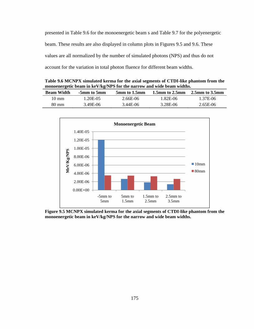
175
presented in Table 9.6 for the monoenergetic beam s and Table 9.7 for the polyenergetic
beam. These results are also displayed in column plots in Figures 9.5 and 9.6. These
values are all normalized by the number of simulated photons (NPS) and thus do not
account for the variation in total photon fluence for different beam widths.
Table 9.6 MCNPX simulated kerma for the axial segments of CTDI-like phantom from the
monoenergetic beam in keV/kg/NPS for the narrow and wide beam widths.
Beam Width -5mm to 5mm 5mm to 1.5mm 1.5mm to 2.5mm 2.5mm to 3.5mm
10 mm 1.20E-05 2.66E-06 1.82E-06 1.37E-06
80 mm 3.49E-06 3.44E-06 3.28E-06 2.65E-06
Figure 9.5 MCNPX simulated kerma for the axial segments of CTDI-like phantom from the
monoenergetic beam in keV/kg/NPS for the narrow and wide beam widths.
0.00E+00
2.00E-06
4.00E-06
6.00E-06
8.00E-06
1.00E-05
1.20E-05
1.40E-05
-5mm to
5mm
5mm to
1.5mm
1.5mm to
2.5mm
2.5mm to
3.5mm
MeV
/Kg
/NP
S
Monoenergetic Beam
10mm
80mm

176
Table 9.7 MCNPX simulated kerma for the axial segments of CTDI-like phantom from the
polyenergetic beam in keV/kg/NPS for the narrow and wide beam widths.
Beam Width -5mm to 5mm 5mm to 1.5mm 1.5mm to 2.5mm 2.5mm to 3.5mm
10 mm 1.36E-05 2.68E-06 1.77E-06 1.31E-06
80 mm 3.71E-06 3.66E-06 3.50E-06 2.79E-06
Figure 9.6 MCNPX simulated kerma for the axial segments of CTDI-like phantom from the
polyenergetic beam in keV/kg/NPS for the narrow and wide beam widths.
The results of the Test 2 simulations to obtain kerma in the center and peripheral
rods from the series of fixed source positions at angular increments of twenty degree
ranging from 0 to 360 degrees are presented in Figure 9.7 on a logarithmic scale. The
kerma values to the central rod had a Coefficient of Variation (standard deviation/mean)
of 0.52%, indicating that this value has almost no dependence on the gantry angle. The
plot in Figure 9.7 indicates a strong sinusoidal relationship between the kerma to the
peripheral rod and the fixed source gantry angle. The actual kerma values for each gantry
angle are reported in units of MeV/kG/NPS in Table 9.8.
0.00E+00
2.00E-06
4.00E-06
6.00E-06
8.00E-06
1.00E-05
1.20E-05
1.40E-05
1.60E-05
-5mm to
5mm
5mm to
1.5mm
1.5mm to
2.5mm
2.5mm to
3.5mm
MeV
/Kg
/NP
S
Polyenergetic Beam
10mm
80mm

177
Figure 9.7 MCNPX simulated kerma tallied in the center and peripheral rods from fixed
source positions at gantry angles ranging from 0 to 360 degrees on a logarithmic scale
1.0E-08
1.0E-07
1.0E-06
1.0E-05
1.0E-04
0 40 80 120 160 200 240 280 320 360
ker
ma
(M
eV/k
g/N
PS
)
Fixed gantry angle (degrees)
Center
Periphery

178
Table 9.8 MCNPX simulated kerma values for the center and peripheral CTDI rod-like
volume from each gantry angle in units of MeV/kG/NPS. The average kerma from angles 0
to 360 is reported for the peripheral rod.
Fixed Gantry Angle Center Rod Peripheral Rod
0 1.217 x 10⁻⁶
1.222 x 10⁻⁵
20 1.226 x 10⁻⁶
1.162 x 10⁻⁵
40 1.221 x 10⁻⁶
9.845 x 10⁻⁶
60 1.213 x 10⁻⁶
6.730 x 10⁻⁶
80 1.212 x 10⁻⁶
2.499 x 10⁻⁶
100 1.219 x 10⁻⁶
6.931 x 10⁻⁷
120 1.209 x 10⁻⁶
2.373 x 10⁻⁷
140 1.220 x 10⁻⁶
1.110 x 10⁻⁷
160 1.224 x 10⁻⁶
7.167 x 10⁻⁸
180 1.231 x 10⁻⁶
5.938 x 10⁻⁸
200 1.226 x 10⁻⁶
6.922 x 10⁻⁸
220 1.224 x 10⁻⁶
1.108 x 10⁻⁷
240 1.222 x 10⁻⁶
2.334 x 10⁻⁷
260 1.215 x 10⁻⁶
6.992 x 10⁻⁷
280 1.217 x 10⁻⁶
2.506 x 10⁻⁶
300 1.224 x 10⁻⁶
6.722 x 10⁻⁶
320 1.213 x 10⁻⁶
9.855 x 10⁻⁶
340 1.233 x 10⁻⁶
1.158 x 10⁻⁵
360 1.217 x 10⁻⁶
1.222 x 10⁻⁵
1.220 x 10⁻⁶
4.214 x 10⁻⁶
The average kerma from the gantry angles ranging from 0 to 340 degrees is also
reported in Table 9.8. The kerma from a single continuous rotation simulation was 1.220
x 10-6
MeV/kg/NPS for the central rod and 4.211 x 10⁻⁶
MeV/kg/NPS peripheral rod. The
percent difference between the average kerma from the discrete source position
simulations and the continuous rotation simulations was 0.054 % for the center rod
0.082% and for the peripheral rod. Again, these errors are both within the reported
statistical error of the MCNPX simulations.

179
9.2.D.4. Discussion
The goal of this set of simulations was to provide researchers a tool to validate
their methods of modeling a rotating fan beam with a given beam width, similar to those
used by CT scanners. Two types of simulations were presented that both utilized a simple
homogenous cylindrical phantom. The results included in Section 9.2.D.3 were all
obtained with the MCNPX transport package and will be submitted for inclusion in the
benchmark data sets that will be in the Task Group 195 report.
The purpose of the Test 1 was to validate the methods used to model the
longitudinal beam profile and did not include source motion. Simulations were performed
to obtain kerma to contiguous axial segments at the center of the CTDI-like phantom.
Results obtained with MCNPX appear to behave as expected. The narrow beam
simulations were performed with a 10 mm wide beam that had a longitudinal range of -5
mm to 5 mm. The kerma from both the monoenergetic and polyenergetic beams to the
axial segment ranging from -5 mm to 5 mm was approximately five times greater than
the kerma in the adjacent segment. Since no primary x-rays reached the other segments,
the kerma to non-directly radiated segments can all attributed to scattered photons from
within the phantom. Conversely, the wide beam was 80 mm and thus covered the entire
range of axial segments. As a result the kerma had less variation across the segments.
Since all segments were directly-irradiated, the decrease in kerma to the more distal
segments can be attributed to the fact that the intensity of a cone beam is inversely
proportional to the square of the distance from the source. As mentioned in Section

180
9.2.D.3, the reported results are all on a per simulated photon basis and so the magnitude
of the doses presented in Figures 9.5 and 9.6 do not reflect the absolute doses to these
segments. In reality, wider collimations would deposit higher doses as the relative fluence
is greater than for narrow collimations.
The purpose of the Test 2 was to validate the rotation of the source about the
isocenter. Simulations were performed to obtain kerma values to the CTDI rod-like
regions at the center and periphery of the cylindrical phantom from a series of
incremental fixed gantry angles. Again, the results obtained with MCNPX simulations
matched what was expected. Due to the symmetry of the rotation and the cylindrical
phantom the kerma to the center rod should be the same regardless of the gantry angle of
the source. As shown in Figure 9.7, the kerma to the center rod was essentially the same
for each simulated gantry angle. As reported above, the variation across all gantry angles
was ~0.5%, which was within the MCNPX reported statistical variation (i.e. simulation
error). The kerma to the peripheral rods should have a sinusoidal dependency on the fixed
gantry angle. The MCNPX results for the peripheral rod exhibited expected periodic
dependence, as shown in Figure 9.7.
Test 2 utilized simulations of several fixed source positions at incremental gantry
angles meant to model a single source rotation. CT simulation codes commonly use an
alternative approach in which the source positions are obtained by randomly sampling a
continuous function. To determine if the results from the set of fixed source simulations
can be used as a benchmark for a package that models a continuous rotation, kerma in the

181
center and peripheral rods was obtained from the UCLA Monte Carlo CT package and
compared to the total kerma from the fixed position source MCNPX simulations. The
percent errors of the total kerma from discrete angle simulations were within the
statistical error of the simulations for both the center and peripheral rod. This indicates
that the average kerma value from set of fixed gantry angle can be used as a validation
benchmark for simulation packages that model rotations using continuous functions
instead of discrete source positions.
9.3 Half Value Layer and Bowtie Profile Measurements as Benchmarks
9.3.A. Introduction
In order to properly model a particular MDCT scanner using Monte Carlo
simulations it is necessary to use a detailed description of the scanner‘s x-ray energy
spectrum, the bowtie and inherent filtration design, and the geometry of the scanner (e.g.
focal spot to isocenter distance, fan angle, z-axis collimation, cone angle settings, etc.).
While it is usually possible to ascertain the geometry of a scanner from documentation,
descriptions of filtration and spectra are generally proprietary. To circumvent this
limitation some groups have worked with scanner manufacturers to obtain spectra and
filtration designs (usually through a non-disclosure agreement)31,33
. Others have used
generic tungsten anode x-ray energy spectra and bowtie filter specifications that are based
on experimentally measurements or theoretical derivations.37
Alternatively, studies have
been performed to examine the utility of obtaining spectrum and filtration schemes based
on measurement. Examples of this method include the equivalent source method

182
described in Chapter 4 and the method developed by McKenney, et al.77
to characterize
bowtie filters using a real-time dose probe.
The most straightforward method to assess a source model‘s accuracy is to
directly compare the results of a simulation with an analogous physical measurement. In
order to isolate the contribution of the source model to the overall simulation accuracy
these type of validation measurements should be made using simple phantoms and source
trajectories (with this approach the errors due to other components of the simulation, such
as inaccuracies in modeling the longitudinal source motion or phantom, are avoided).
Typically, CTDI metrics are used as a benchmark. While these simple simulations
provide some information about a source model‘s precision, it is not clear that they are
sufficient to fully validate a source model. For example, the majority of dose measured
by an ionization chamber in the center of the CTDI phantom is from primary radiation
that passes only through the central ray of the bowtie filter. Thus, on its own, the
CTDI100,center benchmark does not provide adequate confirmation that the filtration across
the fan beam is accurate. Furthermore, if there is significant disagreement between a
CTDI measurement and simulation it is difficult to pinpoint the source of the error (i.e. an
incorrect spectrum, filtration description, or some combination).
The purpose of this work was to compare the sensitivity of conventional CTDI
values to measurements designed to isolate specific components of a scanner-specific
source model. Specifically, the ability of HVL and QVL to assess the spectra and bowtie

183
profile measurements (first introduced in Chapter 4) to evaluate the filtration model will
be investigated as alternative benchmarks to the CTDI.
9.3.B. Methods
For this study, third-generation 64-slice MDCT scanners from two scanner
manufacturers were used (referred to as Scanner 1 and Scanner 2). All the measurements
and simulations described below for each scanner were performed using a protocol of
120 kVp, the widest available collimation setting, and the largest available bowtie. The
mAs setting for each physical measurement was high enough to ensure reproducible
measured values.
All simulations were performed using the UCLA MDCT Monte Carlo simulation
package described in Chapter 3. All MCNPX simulation results were converted to
absolute dose using scanner- and beam width-specific normalization factors, also
described in Chapter 3. For each simulation, enough photon histories were executed to
ensure the reported doses have statistical errors of less than 1% for each tally.
Two different types of x-ray source models, consisting of a photon energy
spectrum and a description of the scanner‘s filtration, were constructed for each scanner.
The first type (denoted Source Model A) consisted of the equivalent source models
generated from scanner-specific measurements, as outlined in Chapter 4. The
HVL&QVL method was used, in which a tungsten anode spectrum was hardened using
various hardening materials until its calculated QVL matched the measured value,

184
resulting in several candidate spectra. Then the spectrum with the calculated HVL that
best matched the measured HVL was deemed the equivalent spectrum. equivalent source
models for Scanners 1 and 2 were referred to as ―Source Model A1‖ and ―Source Model
A2‖, respectively. The second type of source model (denoted Source Model B) was based
on manufacturer provided spectrum and filtration descriptions. These manufacturer
provided source models were referred to as ―Source Model B1‖ and ―Source Model B2‖
for Scanner 1 and 2, respectively.
First, conventional exposure measurements were made on Scanners 1 and 2 in
order to calculate CTDI100,center and CTDI100,periphery for both the 16 cm diameter (head)
and 32 cm diameter (body) CTDI phantom. Analogous simulations were performed,
using geometric descriptions of the CTDI phantoms and ionization chamber, to obtain
simulated CTDI100,center and CTDI100,periphery values using Source Models A1, A2, B1, and
B2. The percent error of each simulated CTDI100 value was calculated relative to the
analogous measured CTDI100 value.
Next, HVL and QVL values were measured on Scanners 1 and 2. HVL was
defined as the thickness of aluminum necessary to reduce the exposure, measured in air at
isocenter, to ½ of the exposure measured with no aluminum present. The QVL was the
thickness of aluminum necessary to reduce the exposure to ¼ of that with no aluminum.
Measurements were obtained for each scanner using a stationary, non-rotating tube
parked at the 6 o‘clock position, as shown in Figure 9.8 (the bed was moved out of the
beam‘s path). An initial exposure measurement was obtained with a 100 mm ionization

185
chamber at isocenter with no aluminum present. Additional exposure measurements were
made, adding thin slabs (0.5–2.0 mm) of type 1100 alloy aluminum in the beam‘s path,
until the HVL and QVL were obtained. Analogous simulations were performed, using
geometric descriptions of the ionization chamber and aluminum slabs, to obtain simulated
HVL and QVL values using Source Models A1, A2, B1, and B2. The percent error of
each simulated HVL and QVL was calculated based on the value of the analogous HVL
and QVL measurements.
Figure 9.8 Diagram of the set up used to measure the HVL and QVL for both Scanners 1
and 2. The x-ray source remained stationary at the 6o'clock position.
Finally, bowtie profile measurements were obtained for Scanners 1 and 2. A
bowtie profile was defined as a set of exposure measurements across the top half of the
fan beam, normalized by the exposure measured at isocenter. All bowtie profile
measurements were made using a stationary, non-rotating tube parked at the 3 o‘clock
position, as shown in Figure 9.9. An initial exposure measurement was obtained with a
100 mm ionization chamber positioned in air at isocenter. Additional exposure

186
measurements were made in air, incrementally moving the scanner bed up in the y-
direction and then each measurement was normalized to the isocenter exposure.
Analogous simulations were performed, using geometric descriptions of the ionization
chamber, to obtain simulated bowtie profiles using Source Models A1, A2, B1, and B2.
The percent error of each simulated bowtie profile value was calculated relative to the
analogous physically measured value.
Figure 9.9 Diagram of the set up used to measure the bowtie profile for both Scanners 1 and
2. The x-ray source remained stationary at the 3 o'clock position.
9.3.C. Results
The percent error of each CTDI100 simulation relative to the actual measured
value is reported in Table 9.9 for all four combinations of scanners and source models
(i.e. Source Model A1, A2, B1, and B2). The root mean square of all the percent errors
for a given scanner/source model combination is listed in the last column. While the
purpose of this study is not to directly compare the source model types, it can be seen

187
that, on average, the percent errors for Source Model A (equivalent source models) are
less than those for Source Model B (manufacturer provided source model).
Table 9.9 The percent error of each CTDI100,center and CTDI100,periphery simulation.
Source
Model
16 cm diameter phantom 32 cm diameter phantom Root Mean
Square Center Periphery Center Periphery
A1 -0.7% 0.2% -3.3% -1.0% 1.8%
A2 6.9% 5.1% -0.5% 1.6% 4.4%
B1 -2.5% -0.2% -8.5% -5.0% 5.1%
B2 -62.1% 31.6% 25.6% 20.4% 38.5%
Table 9.10 shows the percent errors of each HVL and QVL simulation.
Specifically, for each scanner/source model combination, the percent error for the HVL,
QVL, and their root mean square is included. The percent errors for Source Model A are
lower for the QVL values than for the HVL values. This was expected since the
equivalent spectrum was optimized primarily to match the measured QVL. The percent
errors for the source model provided by the manufacturer for Scanner 1 were the smallest
while those for the manufacturer provided model for Scanner 2 were several times greater
than the other source models. It should be noted that the percent errors associated with
the HVL and QVL benchmarks are typically higher than those for the CTDI benchmarks.
Table 9.10 The percent error of each HVL and QVL simulation.
Source Model HVL QVL Root Mean Square
A1 11.2% 4.9% 8.6%
A2 14.5% 6.4% 11.2%
B1 2.7% -1.6% 2.2%
B2 45.1% 34.4% 40.1%

188
The percent errors of the bowtie profile simulation results with respect to the
measured values are shown as a function of the distance from isocenter for each source
model type are shown in Figure 9.10 for Scanner 1 and Figure 9.11 for Scanner 2. The
root mean square of these errors for each scanner and source model combination are
reported in Table 9.11. It can be seen that the root mean square values for Source Model
A are less than those for Source Model B for both scanners. Comparison with Table 9.9
shows that the root mean squares of the simulation errors for the bowtie profile
experiments were not consistently greater or less than those of the CTDI benchmark
experiments.
Figure 9.10 Percent error of bowtie profile simulations as a function the distance from
isocenter (in cm) for Scanner 1.
-20%
-15%
-10%
-5%
0%
5%
0 50 100 150
Distance from isocenter (in cm)
Source Model A1 Source Model B1

189
Figure 9.11 Percent error of bowtie profile simulations as a function the distance from
isocenter (in cm) for Scanner 2.
Table 9.11 The Root Mean Square percent error of each bowtie profile simulation.
Source Model Root Mean Square
A1 1.1
A2 3.9
B1 8.0
B2 23.7
9.3.D. Discussion
This study was conducted to evaluate the sensitivity of CTDI metrics to
benchmark the accuracy of scanner-specific source models. First, it was illustrated that
the CTDI is less sensitive than HVL and QVL benchmarks. Comparisons of Tables 9.9
and 9.10 shows that the root mean squares of the simulation errors were smaller for the
CTDI benchmark experiments compared to the HVL and QVL benchmark experiments
-10%
0%
10%
20%
30%
40%
50%
0 50 100 150 200 250
Distance from isocenter (in cm)
Source Model A2 Source Model B2

190
for almost all source models. This suggests that CTDI metric are less sensitive to
inaccuracies in the source models than HVL and QVL measurements.
Since CTDI100,center, HVL and QVL benchmarks depend primarily on the accuracy
of the spectrum (the majority of the dose for these measurements is due to the portion of
the beam passing through the center of the bowtie filter), bowtie profile measurements
were proposed to assess the accuracy of attenuation across the fan beam. This analysis
revealed that the root mean squares of the simulation errors for the bowtie profile
experiments were not consistently greater or less than those of the CTDI benchmark
experiments. This indicates that summary statistics of the errors from bowtie profile
measurements (such as root mean square) may not be an improvement over CTDI
metrics. However, the percent error profiles presented in Figures 9.10 and 9.11 illustrate
how individual bowtie profile measurements are useful for determining the accuracy of
the bowtie filter model as a function of fan angle.
This analysis illustrated that CTDI metrics are informative and should not be
omitted from a Monte Carlo validation study (i.e. CTDI benchmarks are necessary),
however, it did show that other tests reveal more specific information about the accuracy
of the source model (i.e. CTDI benchmarks are not sufficient). Finally, this work only
included measurements made in air or in a simple, homogenous phantom. Another
sensitivity study should be conducted to investigate the use of more complex,
heterogeneous phantoms for validation purposes.

191
9.4 Surface Dose Measurements on a Thorax Anthropomorphic Phantom
9.4.A. Introduction
The advanced validation methods presented in Sections 9.2 and 9.3 were
developed to assess the accuracy of specific components of a MDCT simulation package,
namely the radiation transport code and x-ray source model. While these are important
initial steps in developing a successful MDCT simulation code, they do not assess
techniques of modeling typical x-ray source trajectories (i.e. helical scans) or methods of
developing detailed patient models.
In order to assess the full simulation package it is necessary to compare
simulations to a dose measurement made using a complex phantom using a complex scan
type. As described above, typical detectors used to measure dose inside a phantoms, such
as TLD‘s, are problematic due to their high energy dependence and the unknown energy
of the hardened beam at the measurement point. As a result, the preferred detector for CT
energies is an ionization chamber, however, they are usually too large to fit inside
anthropomorphic phantoms or the attached wire makes it impossible to properly close the
phantom. The purpose of this study is to address these limitations by investigating the
utility of benchmarking a MDCT Monte Carlo package using a dose measurement from a
helical exam made with an ionization chamber placed on the surface of a phantom.
9.4.B. Methods

192
This study utilized the Alderson Lung/Chest Phantom developed by Radiology
Support Devices, Inc78
. This anthropomorphic thorax phantom extends from the neck to
below the diaphragm and is shown in Figure 9.12. The phantom constructed using the
skeleton of a male patient who is 175 cm tall and weighing 73.5 kg. RSD materials are
equivalent to natural bone and soft tissues.78
Animal lungs selected to match the size of
the adult male are fixed in their inflated state and molded to fit inside the pleural cavities
of the phantom and the blood vessels are filled with blood equivalent plastic.
Figure 9.12 The Alderson Chest/Lung Phantom from Radiological Support Devices, INC.
78
The RadCal modern wide beam multi-slice CT chamber (0.6-cc active volume)79
was used to measure dose for this study. This chamber was used with the RadCal Accu-
Pro Multi Purpose meter and was calibrated by the manufacturer using 150 kVp x-rays.79
This small ionization chamber was taped to the anterior of the chest phantom, just below
the shoulder region at the center of the coronal plane.

193
Dose was measured on a Siemens Sensation 64 scanner from 120 kVp helical
scans of pitch 1.5, nominal beam width of 28.8 mm, and effective mAs of 150 (tube
current modulation was not used). The scan region was defined using a topogram image.
The extent of the image data was 17.4 cm however there was 3.5 cm of z-overscan on
each side so the total irradiation length was 24.4 cm. The table height was adjusted so
that the center of the phantom was approximately in the center of the CT gantry and 25
dose measurements were obtained. Since the start angle for scans on the Siemens
Sensation 64 is random the relative position of the source when passing over the
ionization chamber varied for each separate measurement. The start angle for each scan
was retrieved from the raw data.
A voxelized model of the thorax phantom was created from the image data from
one of the scans using the methods developed by Angel, et al.61,62
and described in detail
in Chapter 8. Each voxel in the image was mapped to one of five anatomical materials
including soft tissue, lung, water, fat, or bone. This process is illustrated in Figure 9.13.

194
Figure 9.13 Generation of a voxelized model: (a) original patient image, (b) radiologist’s
contour of the breast region, (c) threshold image to identify glandular breast tissue and (d)
the resulting voxelized model. Reprinted from Angel, et al.61,62
.
Since the Alderson Chest/Lung phantom was constructed using tissue equivalent
materials, each of tissue type was assigned a single elemental composition and density
corresponding to the definitions specified in ICRU Report 4455
. Additionally, the wall
and air inside the ionization chamber were separately contoured by hand. In order to
obtain sufficient resolution to tally within the air portion of the ionization chamber it was
not possible to sub-sample the images when creating voxelized models. As a result each
axial slice consisted of a 512 x 512 array of material numbers. Each voxel was 0.8 mm
0.8 mm and the slice thickness was 1.5 mm. A series of illustrations of the high-
resolution voxelized phantom are shown in Figures 9.14-9.16. The green portion of the
ionization chamber represents the air tally region. As can be seen from these figures, the
scanner bed was mapped to various tissue types based on the CT number.

195
Figure 9.14 Axial view of the voxelized model created from images of the Alderson
Lung/Chest Phantom.
Figure 9.15 Sagital view of the voxelized model created from images of the Alderson
Lung/Chest Phantom.
Tally Region
Tally Region

196
Figure 9.16 Coronal view of the voxelized model created from images of the Alderson
Lung/Chest Phantom.
The UCLA MDCT Monte Carlo dosimetry package was used to simulate the dose
to the air inside the tally region from the helical scans. The longitudinal start and stop
locations for the simulations coincide with the boundaries of the voxelized phantom. As
mentioned above, the actual start and stop locations of the scans do not coincide with the
image data due to the 3.5 cm of z-overscan on each side. In order to ensure that the
helical path of the simulations was in phase with the actual measurement it was necessary
to determine the correct start angle for the simulations. The tube angle recorded from the
raw data corresponds to the angle at which the tube actually turned on, not the angle of
the tube at the start of the image data. So, the number of degrees that the source rotated
during the initial overscan was calculated based on the overscan distance, collimation
width, and pitch. Then, the proper simulated start angle (SAsim) was obtained by adding
Tally Region

197
the overscan rotation to the actual tube start angle (SAactual). The simulated tube start
angle was obtained from Equation 9.8:
Eq. 9.8
For the helical scans used to measure dose on the thorax phantom, the last two terms was
equal to 291.67 degrees.
Dose was obtained in mGy/NPS by tallying the energy fluence in the air portion
of the ionization chamber and converting to kerma using the energy-dependent mass-
energy absorption coefficients for air45
. Next, the appropriate scanner- and collimation-
dependent normalization factor was used to convert these results to dose in mGy/total
mAs. Then, the absolute dose in mGy was obtained by multiplying by the total mAs,
which is the product of the effective mAs (150), the total number of simulated rotations
(4.0278), and the pitch (1.5). Finally, the percent error of the simulated dose was
calculated for each tube start angle relative to the dose measured with the ionization
chamber.
9.4.C. Results
The measured and simulated dose values obtained with the ionization chamber on
the surface of the thorax phantom is reported in Table 9.12 for each actual tube start
angle. The last column shows the percent error of the simulated dose with respect to the
measured dose. The root mean square of the percent errors is 6.6%.

198
Table 9.12 The measured and simulated doses to the ionization chamber located on the
surface of the thorax phantom and the simulation percent error for each actual start angle.
Tube Start Angle Measured Dose
(mGy)
Simulated Dose
(mGy) Simulation % Error
291.72 10.07 9.26 -8.0%
355.03 11.36 11.70 3.0%
99.31 17.70 18.31 3.5%
6.2069 12.01 12.74 6.1%
281.79 10.42 9.40 -9.8%
219.72 14.24 13.08 -8.1%
255.72 11.72 10.44 -10.9%
84.414 17.07 17.67 3.5%
214.76 14.50 13.18 -9.1%
194.9 16.38 14.92 -8.9%
333.93 10.30 10.20 -1.0%
153.93 17.96 17.55 -2.3%
357.52 11.51 11.96 3.9%
114.21 18.22 18.88 3.6%
99.31 17.78 18.31 3.0%
198.62 15.77 14.37 -8.8%
202.34 15.28 14.44 -5.5%
356.28 11.41 11.88 4.1%
222.21 13.96 12.73 -8.9%
230.9 13.32 12.27 -7.9%
106.76 18.05 18.63 3.2%
269.38 11.00 9.70 -11.8%
24.828 13.26 13.62 2.7%
27.31 13.44 13.92 3.6%
A plot of the measured and simulated doses as a function of start angle is shown Figure
9.17. From this plot it can be seen that there appears to be a alight phase shift between the
simulated and measured doses.

199
Figure 9.17 The measured and simulated doses to the ionization chamber located on the
surface of the thorax phantom as a function of tube start angle.
9.4.D. Discussion
This work was performed to investigate the feasibility of using a surface dose
measurement made with a small ionization chamber placed on an anthropomorphic
phantom as a Monte Carlo simulation benchmark. These measurements were made using
a helical scan (with a pitch of 1.5) on a Siemens Sensation 64 scanner. This
benchmarking method overcomes many limitations of other, commonly utilized
validation techniques. First, the dose measurement was made with an ionization chamber
which has been shown to be energy independent, even in the diagnostic ranges. This
0
2
4
6
8
10
12
14
16
18
20
0 40 80 120 160 200 240 280 320 360
Do
se (
mG
y)
Tube Start Angle (degree)
Measured Simulated

200
immediately represents an improvement over studies that attempt to quantify absolute
dose with energy-dependent solid state detectors, TLD‘s, MOSFET‘s, OSL‘s, etc.
Second, this validation metric is comprehensive in that all the components of the
simulation package must be accurate in order to obtain a simulation result that matches
the measurement. This includes the radiation transport code, the scanner-specific x-ray
source, the longitudinal beam profile model, the methods used to model a rotating and
translating source, and the techniques used to build a voxelized patient model from image
data.
The results of this exercise illustrated that it is possible to obtain simulation
accuracies with a root mean square error of less than 10% across a number of different
starting conditions (i.e. tube start angle). The error of the simulations with respect to the
measurements for all 24 of the tube start angles are reported in Table 9.12. It has been
suggested that for complex CT dose simulations that incorporate a high number of
parameters that influence the results, simulation with errors of up to 20% can be
considered accurate.71
The maximum absolute error reported in Table 9.12, was 11.8%,
which is well within the 20% criterion.
While it is probably sufficient to attribute the simulation error to inaccuracies in
various levels of the simulation chain (i.e. imprecise spectra, filtration descriptions,
patient modeling techniques, etc.), the plot shown in Figure 9.17 indicates another
potential source of error. From this plot it appears there is a phase shift between the

201
simulated and measured values as a function of tube start angle. A phase shift suggests
that, for a given tube start angle, the lateral location of the ionization chamber in the
simulations may have been slightly different than that of the actual measurements. A
diagram to illustrate this principle is presented in Figure 9.18. This cartoon shows both a
centered phantom and one slightly shifted laterally to the left. For a specific tube start
angle, assume the source was at the 12 o‘clock position when passing directly over the
chamber (red source). This source position will result in the maximum dose to the green
chamber. It can be seen that the distance between the red source and the yellow chamber
(black arrow) is longer than the distance between the red source and the green chamber.
Thus the green chamber will receive a higher dose for that particular start angle because
of the inverse square law. Now, when the x-ray tube is located at the blue source position
the same argument can be used to show that the yellow chamber gets a higher dose. In
fact, it can be seen that the blue arrow (maximum dose to yellow chamber) is shorter than
the red arrow (maximum dose to green chamber). This indicates that the maximum dose
to the yellow chamber is greater than the maximum dose to the green chamber. A similar
argument can be made to show that the minimum dose to the yellow chamber is less than
the minimum dose to the green. In conclusion, the dose as a function of start angle for the
laterally shifted phantom will have a greater amplitude and be phase shifted in
comparison that of a centered phantom. The plot in Figure 9.17 shows this exact
behavior, indicating a lateral shift between the simulated and measured data. This
illustrates the importance of exactly recreating the measurement set up with the

202
simulation geometry for a validation study as intricate and detailed as the voxelized
thorax phantom benchmark described above.
Figure 9.18 Diagram to illustrate how a lateral shift results in a phase shift and amplitude
change for dose as a function of tube start angle plot.
This study utilized a helical scan performed with a constant tube current. It is
feasible that this method could be extended in order to validate simulations of TCM
exams. The same measurement procedure could be used to measure the dose from a
helical exam performed with TCM. The resulting dose value would serve as benchmark
for simulations that account for TCM, such as the one described in detail in Chapter 8.

203
This would represent one of the first attempts to assess the accuracy of TCM simulations
by direct comparison to physical dose measurements and should be addressed in future
work.
9.5 Conclusions
The focus of this chapter was on developing advanced benchmarks for validating
MDCT Monte Carlo dosimetry codes. It is difficult to establish standard validation
methodologies due to the large variation in Monte Carlo radiation transport codes and
the often misunderstood issues involved with properly calibrating physical dose detectors
at diagnostic energies (including TLD‘s, MOSFET‘s, and OSL‘s).
First, the reference test cases currently being generated by the AAPM Task Group
195 were summarized and the results obtained with the MCNPX simulation package for
the HVL/QVL and CTDI with Simple Phantoms test cases were presented. It was
demonstrated that these reference simulations can be performed using standard CT
modeling methods and that the results produced with the MCNPX transport code
matched expected results. Thus, the data presented in Section 9.2 can be used for
comparisons to assess the relative performance of other types of Monte Carlo radiation
transport codes. This work represents the first standardized set of Monte Carlo
simulations specifically designed for validation of common diagnostic imaging tasks.
When completed, the data included in the Task Group 195 Report will serve as a valuable

204
tool for researchers developing their own Monte Carlo codes or learning how to do
Monte Carlo simulations.
Next, a set of more sophisticated measurements for assessing the accuracy of
scanner-specific x-ray source models was proposed. Specifically, the goal of this exercise
was to determine better methods of assessing the x-ray energy spectrum and filtration
description based on measurements made on the scanner of interest. These benchmarks
consisted of HVL, QVL, and bowtie profile measurements. In order to avoid issues with
improper calibration, absolute dose measurements were all acquired with a 100 mm
ionization chamber. Since all three of these metrics are obtained with a parked x-ray
source, the accuracy of the analogous simulation s primarily depends on the accuracy of
the scanner-specific source model for the scanner of interest. It was shown that the HVL
and QVL measurements are more sensitive than common CTDI validation techniques
and thus can be considered a higher order check of the x-ray source model accuracy. The
bowtie profile measurements provide extra spatial information to evaluate the accuracy of
the filtration model that provides attenuation across the fan beam. This work was not
meant to suggest that CTDI validation techniques should be ignored; however, additional,
higher-order benchmarking should also be included in order to gain more specific
information about the specific source of potential simulation errors.
Finally, a more comprehensive benchmark measurement was proposed using a
small volume ionization chamber and a complex, anthropomorphic phantom. Dose from
a helical exam was measured using the ionization chamber which was fixed to the surface

205
of the Alderson Chest/Lung phantom. A large number of measurements were obtained,
all at different tube start angles. In order to accurately simulate these dose values it was
necessary to obtain an accurate voxelized patient model and scanner-specific x-ray source
information and to utilize a precise source trajectory model. Simulation results obtained
with the UCLA MDCT Monte Carlo package discussed in Chapters 3 and 4 were, on
average, within 10% of measured dose values. The power of this validation methodology
is the fact that the overall simulation error is due to the propagation of errors introduced
by the inaccuracies of the various simulation components. While a test like this is not
extremely useful for diagnosing where errors are coming from, it is the best indicator of
how well a simulation package can accurately obtain the dose to specific points on an
actual patient model. This approach could also be used to validate the method of
modeling tube current modulation by repeating the same steps but for a helical exam
performed with TCM.
It is clear that in order to produce credible results the accuracy of Monte Carlo CT
simulation packages must be properly validated. The advanced validation methods
presented in this chapter were each developed to assess specific components of a CT
simulation model. These benchmarks should be used to evaluate the accuracy of a code
from the ground up, starting with the radiation transport, then the x-ray source model,
then a simple rotating source with no translation, and finally a full helical and/or
translating axial scan.

206
A suggested path for robustly validating a Monte Carlo code along with some
specific benchmarks is presented in Figure 9.19. Starting at the top, each level should be
addressed individually until the accuracy of each major component of the simulation
package is successfully demonstrated. It is certainly possible to develop other types of
tests to assess each level‘s main component and to add more levels to this validation map;
however, this type of comprehensive approach to validation should be a prerequisite
before assuming the validity of simulation results obtained with CT Monte Carlo
packages.

207
Figure 9.19 Proposed approach for robustly validating the accuracy of a Monte Carlo CT
simulation package. Starting at the top, each level introduces a new level of complexity in
order to assess a different component of the simulation package.
Scanner-Specific Tube Current Modulation model
Dose measured with ion chamber on surface of heterogeneous anthropomorphic phantom for a TCM helical exam (extension of Section 9.4)
Scanner-specific helical source motion model and patient modeling techniques
Dose measured with ion chamber on surface of heterogeneous anthropomorphic phantom for a fixed tube current helical exam (Section 9.4)
Scanner-specific single rotation model with a simple phantom
Measured center and peripheral CTDI100 with head and body CTDI phantoms (Chapter 4)
Scanner-specific source model (energy spectrum and filtration)
Measured HVL, QVL, and bowtie profile benchmarks (Section 9.3)
Dose distribution in a simple voxelized patient with a generic scanner model
AAPM Task Goup 195 CT Dosimetry in Voxelized Patient Models Test Case (currently being developed)
Beam width model and rotation about isocenter model with a generic scanner
AAPM Task Group 195 CT Dosimetry in Simple Volumes (Section 9.2.D)
Radiation Transport Code
AAPM Task Group 195 HVL and QVL Test Case (Section 9.2.C)

208
Chapter 10 Dissertation Summary and Conclusions
This purpose of the work presented in this dissertation was to extend the field of
CT dosimetry by introducing novel methods of evaluating dose to patients. It was
established that the currently accepted clinical dose measurement paradigm, namely the
CTDI, is not a direct measurement of the preferred dose evaluation metric, the dose to
individual organs. In this dissertation, Monte Carlo simulations were heavily utilized to
obtain the dose to organs in detailed patient modes; however, the necessity of
individualized segmented organs makes it infeasible to perform such simulations on all
patients undergoing CT exams. Instead, the goal was to develop a generalizable organ
dose estimation method that could actually be used in a clinical setting based on readily
available information about the radiation output from the scanner and the size of the
patient.
Chapters 3 and 4 described the intricate details of the UCLA MDCT Monte Carlo
dosimetry package. Since the modeling of a specific scanner requires an accurate
description of the x-ray energy spectrum and filtration design (including bowtie filter)
and this information is difficult to obtain for specific scanners, an algorithm to generate
―equivalent x-ray source models‖ was developed. This methodology, presented in
Chapter 4, can be used to create source models for any scanner as it is based solely on
measured data. The high accuracy of simulations performed using the equivalent source
models was demonstrated using both common validation techniques (i.e. CTDI) as well
as the advanced benchmark metrics described in Chapter 9.

209
The advent of the equivalent source models made it possible to simulate any
MDCT scanner. As a result the work presented in Chapter 5 represented the first study
that compared the organ doses from different MDCT scanners under comparable scan
protocols. It was shown that, while absolute organ doses varied considerably, organ doses
normalized by measured CTDIvol values had very small variations across scanners. Thus
the average CTDIvol normalized organ dose value across scanners served as an accurate
approximation for any given scanner. This finding demonstrated the feasibility of
generating scanner-independent CTDIvol-to-organ dose conversion coefficients for
individual patients.
The study presented in Chapter 6 was conducted in order to investigate the
dependence of CTDIvol-to-organ dose conversion coefficients on patient size. It was
established that a strong decreasing exponential correlation exists with patient perimeter
for all organs fully encompassed in the scan region. Exponential fit parameters that are
specific to the type of scan (i.e. abdominal, chest, pelvis, etc) were determined for each
organ (denoted AO and BO) which can be used to calculate a CTDIvol-to-organ dose
conversion coefficient for any patient based on the perimeter of the central slice in the
scan region. Then, with a knowledge of the CTDIvol reported by the scanner for that
exam, a set of patient-, scanner-, and exam-specific organ doses can be obtained.
Chapters 7 and 8 describe a pair of studies that extend the organ dose estimation
technique to include organs only partially encompassed in the scan region and to account

210
for dose reductions due to tube current modulation. An expression to estimate dose to
partially-irradiated organs was derived in Chapter 7 that made several assumptions
regarding the individual doses to the portion of the organ inside and outside the scan
region. It was demonstrated that even though these assumptions are not always
completely satisfied, the partially-irradiated dose estimates are reasonably accurate,
especially when compared to the alternative dose evaluation, the CTDI. The work in
Chapter 8 illustrated a method to calculate patient-specific TCM correction factors for
dose estimates to fully-irradiated organs.
The major limitation that affected all of the organ dose studies was the small
number of available patient models with full sets of contoured organs. Only eight fully
segmented models (the GSF Family of Voxelized Phantoms) were available. Since these
models spanned a large range of ages and included both males and females, it was not
possible to obtain good enough statistics to generate dose estimation coefficients for
particular anatomical regions, namely the chest (inclusion of breast tissue) and pelvis (i.e.
variation in gonads and other gender-specific organs). The small number of patient
models also made it impossible to properly assess the accuracy of the dose estimation
method using training and testing patient model subsets. Currently, the number of UCLA
voxelized patient models, similar to those described in Chapter 8, are being constructed
and will be utilized to obtain dose estimation coefficients for anatomical regions other
than the abdomen and to rigorously validate the accuracy of the dose estimation method.

211
In conclusion, the culmination of the work presented in this dissertation
demonstrated the feasibility of a method to estimate dose to fully- and partially-irradiated
organs for fixed or modulated tube current exams from any scanner to any patient. An
overview of this method along with the necessary coefficients derived in this manuscript
is presented in Appendix C.
Since the required inputs to the proposed organ dose estimation method only are
either readily available (estimation coefficients summarized in Appendix C and the
CTDIvol included in the CT dose report) or relatively easily attainable (patient perimeter),
it is reasonable to suggest that doses to organs should be calculated on a routine clinical
basis. Work is already being done to include organ dose estimates in a DICOM dose
structure report which can be stored to commercial PACS systems and potentially used to
track the dose and even the risk to patients associated with CT exams.

212
Appendix A. Supplementary Tables from Chapter 4
Table 4.3 – Scanner/Bowtie Combination A – CTDI100 results across all kVp’s, phantom
sizes and positions for both measured and simulated results. Simulated results are from all
three source models: (a) source based on manufacturer-provided data, (b) equivalent source
model based on HVL method and (c) equivalent source model based on HVL&QVL
method. Percent difference values are the percent difference between simulated and
measured for each source model method.
% difference between simulated CTDI100 and
measured CTDI100
kVp Chamber
position
Measured
CTDI100
(mGy/mAs)
Manufacturer-
based source
model
HVL source
model
HVL&QVL
source model
16
cm
CT
DI
Ph
an
tom
80 center 0.036 -4.59 -3.05 -4.34
12:00 0.039 2.64 4.10 -1.81
100 center 0.075 -3.73 -2.70 -1.86
12:00 0.081 -0.78 0.78 -1.21
120 center 0.131 -2.51 -1.45 -0.67
12:00 0.140 -0.20 -0.47 -0.43
140 center 0.199 -2.83 -3.01 -1.28
12:00 0.212 0.03 -2.39 0.78
32
cm
CT
DI
Ph
an
tom
80 center 0.010 -10.27 -7.29 -10.76
12:00 0.021 -5.15 11.06 -4.92
100 center 0.024 -10.24 -8.09 -7.38
12:00 0.045 -5.47 1.29 -4.46
120 center 0.044 -8.50 -7.04 -3.67
12:00 0.081 -5.05 -3.20 -3.04
140 center 0.070 -6.36 -6.95 -2.71
12:00 0.125 -4.65 -7.87 0.34
Root Mean Square % Difference: 5.50 5.38 4.14

213
Table 4.4 – Scanner/Bowtie combination B - CTDI100 results across all kVp’s, phantom sizes
and positions for both measured and simulated results. Simulated results are from all three
source models: (a) source based on manufacturer-provided data, (b) equivalent source
model based on HVL method and (c) equivalent source model based on HVL&QVL
method. Percent difference values are the percent difference between simulated and
measured for each source model method.
% difference between simulated CTDI100 and
measured CTDI100
kVp Chamber
position
Measured
CTDI100
(mGy/mAs)
Manufacturer-
based source
model
HVL source
model
HVL&QVL
source model
16
cm
CT
DI
Ph
an
tom
80 center 0.061 13.09 3.92 8.30
12:00 0.073 13.44 10.68 12.34
100 center 0.120 11.12 1.32 3.26
12:00 0.139 10.00 3.78 4.24
120 center 0.186 8.75 1.70 0.99
12:00 0.206 11.51 4.50 4.46
135 center 0.243 6.44 1.68 0.20
12:00 0.276 6.28 -1.04 -1.55
32
cm
CT
DI
Ph
an
tom
80 center 0.015 16.09 0.66 7.62
12:00 0.035 10.01 17.30 18.48
100 center 0.034 12.82 -4.96 -1.25
12:00 0.068 8.94 5.64 6.05
120 center 0.058 10.31 -5.27 -5.53
12:00 0.108 6.98 -1.94 -1.60
135 center 0.078 10.66 -7.31 -7.96
12:00 0.139 8.25 -3.53 -4.28
Root Mean Square % Difference: 10.62 6.25 7.18

214
Table 4.5 – Scanner/Bowtie combination C - CTDI100 results across all kVp’s, phantom sizes
and positions for both measured and simulated results. Simulated results are from all three
source models: (a) source based on manufacturer-provided data, (b) equivalent source
model based on HVL method and (c) equivalent source model based on HVL&QVL
method. Percent difference values are the percent difference between simulated and
measured for each source model method.
% difference between simulated CTDI100 and
measured CTDI100
kVp Chamber
position
Measured
CTDI100
(mGy/mAs)
Manufacturer-
based source
model
HVL source
model
HVL&QVL
source model
16
cm
CT
DI
Ph
an
tom
80 center 0.058 18.51 -4.49 -2.37
12:00 0.073 9.06 -0.77 -0.25
100 center 0.112 10.69 -4.57 -2.74
12:00 0.134 5.48 -0.74 0.26
120 center 0.177 7.46 -4.41 -4.28
12:00 0.209 2.54 -2.63 -2.59
140 center 0.252 2.77 -4.51 -0.72
12:00 0.292 0.35 -3.06 -1.53
32
cm
CT
DI
Ph
an
tom
80 center 0.016 31.31 -10.10 -7.03
12:00 0.043 0.07 -6.51 -5.77
100 center 0.034 22.74 -9.57 -6.40
12:00 0.077 2.13 -3.88 -3.41
120 center 0.056 16.64 -7.09 -6.86
12:00 0.116 2.84 -3.38 -3.38
140 center 0.083 10.60 -4.20 -0.54
12:00 0.165 -0.44 -6.01 -4.78
Root Mean Square % Difference: 12.60 5.39 4.02

215
Table 4.6 – Scanner/Bowtie combination D - CTDI100 results across all kVp’s, phantom sizes
and positions for both measured and simulated results. Simulated results are from all three
source models: (a) source based on manufacturer-provided data, (b) equivalent source
model based on HVL method and (c) equivalent source model based on HVL&QVL
method. Percent difference values are the percent difference between simulated and
measured for each source model method.
% difference between simulated CTDI100 and
measured CTDI100
kVp Chamber
position
Measured
CTDI100
(mGy/mAs)
Manufacturer-
based source
model
HVL source
model
HVL&QVL
source model
16
cm
CT
DI
Ph
an
tom
80 center 0.032 -- -2.85 -2.08
12:00 0.038 -- 1.80 2.02
100 center 0.111 -1.61 0.06 -0.03
12:00 0.124 2.81 0.93 1.20
140 center 0.162 -- -1.29 -1.06
12:00 0.180 -- 0.38 0.39
32
cm
CT
DI
Ph
an
tom
80 center 0.009 -- -4.22 -3.00
12:00 0.023 -- 1.48 1.45
100 center 0.037 -3.48 -2.65 -0.81
12:00 0.075 1.92 -3.58 -3.46
140 center 0.057 -- -2.04 -0.97
12:00 0.110 -- -5.78 -6.36
Root Mean Square % Difference: 2.56 2.76 2.52

216
Table 4.7 – Scanner/Bowtie combination E - CTDI100 results across all kVp’s, phantom sizes
and positions for both measured and simulated results. Simulated results are from all three
source models: (a) source based on manufacturer-provided data, (b) equivalent source
model based on HVL method and (c) equivalent source model based on HVL&QVL
method. Percent difference values are the percent difference between simulated and
measured for each source model method.
% difference between simulated CTDI100 and
measured CTDI100
kVp Chamber
position
Measured
CTDI100
(mGy/mAs)
Manufacturer-
based source
model
HVL source
model
HVL&QVL
source model
16
cm
CT
DI
Ph
an
tom
80 center 0.066 -13.98 -4.08 -0.34
12:00 0.075 -11.20 0.75 2.27
100 center 0.122 -11.80 -4.54 -2.73
12:00 0.130 -9.74 -0.79 -0.19
120 center 0.188 -9.70 -4.83 -1.46
12:00 0.197 -8.59 -2.94 -1.75
140 center 0.263 -10.53 -5.49 0.70
12:00 0.273 -8.96 -5.63 -3.38
32
cm
CT
DI
Ph
an
tom
80 center 0.015 -13.19 1.39 6.76
12:00 0.036 -14.10 7.77 8.86
100 center 0.031 -11.79 0.08 4.81
12:00 0.066 -15.84 -1.57 -0.55
120 center 0.051 -10.70 -2.90 2.32
12:00 0.097 -12.16 -2.38 -1.98
140 center 0.076 -11.58 -5.59 3.05
12:00 0.137 -12.90 -7.38 -5.88
Root Mean Square % Difference: 11.83 4.31 3.80

217
Table 4.8 – Scanner/Bowtie combination F - CTDI100 results across all kVp’s, phantom sizes
and positions for both measured and simulated results. Simulated results are from all three
source models: (a) source based on manufacturer-provided data, (b) equivalent source
model based on HVL method and (c) equivalent source model based on HVL&QVL
method. Percent difference values are the percent difference between simulated and
measured for each source model method.
% difference between simulated CTDI100 and
measured CTDI100
kVp Chamber
position
Measured
CTDI100
(mGy/mAs)
Manufacturer-
based source
model
HVL source
model
HVL&QVL
source model
16
cm
CT
DI
Ph
an
tom
80 center 0.084 23.94 4.15 6.85
12:00 0.110 18.23 12.00 13.01
100 center 0.152 21.31 3.01 4.58
12:00 0.183 17.89 7.04 7.43
120 center 0.227 19.64 3.66 6.86
12:00 0.265 18.07 3.64 5.05
135 center 0.292 13.71 1.47 2.49
12:00 0.349 9.50 -3.48 -2.59
32
cm
CT
DI
Ph
an
tom
80 center 0.020 29.94 -1.82 2.40
12:00 0.057 19.99 21.79 22.05
100 center 0.042 26.66 -4.76 -2.23
12:00 0.103 17.01 6.29 6.54
120 center 0.069 25.57 -4.16 -0.46
12:00 0.150 20.43 0.71 1.59
135 center 0.092 21.79 -7.49 -5.72
12:00 0.176 27.95 4.99 5.01
Root Mean Square % Difference: 20.18 7.40 7.72

218
Table 4.9 – Scanner/Bowtie combination G - CTDI100 results across all kVp’s, phantom sizes
and positions for both measured and simulated results. Simulated results are from all three
source models: (a) source based on manufacturer-provided data, (b) equivalent source
model based on HVL method and (c) equivalent source model based on HVL&QVL
method. Percent difference values are the percent difference between simulated and
measured for each source model method.
% difference between simulated CTDI100 and
measured CTDI100
kVp Chamber
position
Measured
CTDI100
(mGy/mAs)
Manufacturer-
based source
model
HVL source
model
HVL&QVL
source model
16
cm
CT
DI
Ph
an
tom
80 center 0.070 -13.07 -4.81 -0.91
12:00 0.088 -7.75 -0.40 1.28
100 center 0.130 -10.81 -2.31 -2.31
12:00 0.153 -7.83 -1.34 -1.34
120 center 0.200 -8.81 -0.76 -0.76
12:00 0.230 -6.49 -1.60 -1.60
135 center 0.279 -9.75 -5.06 -1.43
12:00 0.311 -5.34 -3.19 -1.71
32
cm
CT
DI
Ph
an
tom
80 center 0.016 -12.04 -0.73 4.76
12:00 0.043 -9.84 6.16 7.40
100 center 0.034 -10.24 4.76 4.76
12:00 0.077 -9.08 2.31 2.31
120 center 0.056 -8.93 3.35 3.35
12:00 0.116 -8.21 -1.40 -1.40
135 center 0.083 -10.19 -5.45 -0.50
12:00 0.165 -10.75 -7.94 -6.75
Root Mean Square % Difference: 9.51 3.89 3.37

219
Appendix B. Energy Dependence of Small Volume Ionization Chambers and Solid
State Detectors at Diagnostic Energy Ranges for CT Dosimetry – Assessment In Air
and In Phantom
Introduction
AAPM Task Group 111 has described a new methodology for measuring the dose
profile from CT exams to address the limitations of conventional 100 mm ionization
chambers. Their report suggests the use of ―a conventional thimble ionization chamber
with… a flat energy response (~1.5% variation) over the HVL range 2–15 mm Al and
which is calibrated by an accredited dosimetry calibration laboratory (ADCL) for ranges
of beam quality and kVp (80–140 kVp) associated with those of CT‖13
. Ionization
chambers are typically calibrated at higher energy levels. Since then, solid state detectors
with even smaller active lengths have also become a viable option. However, a
comprehensive investigation of the energy response of commercial small ionization
chambers and solid state detectors has not been published.
Reference chamber: PTW Farmer Ionization chamber with a sensitive volume of 0.6-cc
that has been calibrated by the University of Wisconsin ADCL using beams with HVL‘s
ranging from 2.96 to 10.2 mm Al. A polynomial function was obtained to describe the
calibration factor (NK) as a function of HVL:
HVL ADCL NK (x109 cGy/C)
2.96 4.722
4.98 4.663
6.96 4.641
10.2 4.685

220
Polynomial Regression:
Test Ionization Chamber: RadCal modern wide beam multi-slice CT chamber (0.6-cc
active volume). This chamber was used with the RadCal Accu-Pro Multi Purpose meter
and was calibrated by the manufacturer using 150 kVp x-rays.
Test Solid State Dosimeter: RTI CT Dose Profiler uses a solid-state chip with an active
length of 0.3 mm that has negligible angular dependence. Used with the RTI Barracuda
multimeter.
Half-value Layer: HVL‘s (mm Al) were obtained for the Siemens SOMATOM
Sensation 64 and the Toshiba Aquilion 64. The HVL of the beam was measured in-air
using a simple, fixed-tube approach. The HVL of the beam at the center of both head (16
cm diameter) and body (32 cm diameter) CTDI phantoms were determined using Monte
4.6
4.65
4.7
4.75
0 3 6 9 12
HVL in mm Al
ADCL Nk (x10^9 cGy/C)

221
Carlo simulations (these simulations are the subject of a separate AAPM conference
submission). For each HVL, a corresponding NK was calculated using the regression
equation above in order to precisely determine absolute dose values with the reference
chamber.
Toshiba Aquilion 64
kVp In-Air Head CTDI Phantom Body CTDI Phantom
HVL NK HVL NK HVL NK
80 3.49 4.703 3.14 4.715 2.80 4.729
100 4.47 4.675 4.03 4.687 3.58 4.700
120 5.45 4.655 4.91 4.665 4.36 4.678
135 6.10 4.648 5.49 4.655 4.88 4.666
Siemens SOMATOM Sensation 64
kVp In-Air Head CTDI Phantom Body CTDI Phantom
HVL NK HVL NK HVL NK
80 6.20 4.647 5.60 4.653 5.30 4.658
100 7.80 4.646 6.80 4.644 6.20 4.647
120 8.70 4.656 7.90 4.647 7.20 4.643
140 9.70 4.676 8.80 4.657 7.90 4.647
Methods: Doses were measured for single axial scans with the dosimeter at the isocenter.
The widest collimation setting was used to ensure the active portion of each dosimeter
was fully-irradiated (Siemens: 24 x 1.2 mm and Toshiba: 8 x 5.0 mm). Measurements
were also made in-air and in the center of the head and body CTDI phantoms. For each
kVp on both scanners, the mAs value necessary to produce the same measurement using
the reference chamber as the 80kVp/500mAs condition was established for in-air and in-
phantom set-ups. The same conditions were used for the two test chambers.

222
Results:
Head (16 cm diameter) CTDI Phantom Measurements
Scan Parameters Reference
Test 0.6-cc Ionization
Chamber
Test Solid State
Dosimeter
kVp HVL mAs mGy mGy
% error
relative to
Reference
mGy
% error
relative to
Reference
To
shib
a
80 3.14 500 19.84 20.50 3.2% 22.46 13.2%
100 4.03 280 19.70 20.32 3.1% 21.34 8.3%
120 4.91 180 19.02 19.97 4.8% 20.11 5.8%
135 5.49 140 19.33 20.15 4.0% 19.73 2.1%
Sie
men
s
80 5.60 500 8.82 9.26 4.9% 10.66 20.8%
100 6.80 240 8.82 9.25 4.8% 9.91 12.3%
120 7.90 145 8.92 9.24 3.6% 9.35 4.8%
140 8.80 92 8.84 9.21 4.2% 8.60 -2.7%
Body (32 cm diameter) CTDI Phantom Measurements
Scan Parameters Reference
Test 0.6-cc Ionization
Chamber
Test Solid State
Dosimeter
kVp HVL mAs mGy mGy
% error
relative to
Reference
mGy
% error
relative to
Reference
Tosh
iba
80 2.80 500 3.90 4.20 7.3% 5.33 36.7%
100 3.58 250 3.81 4.25 10.4% 5.13 34.8%
120 4.36 150 3.72 4.21 11.6% 4.93 32.3%
135 4.88 110 3.67 4.16 11.8% 4.80 30.8%
Sie
men
s
80 5.30 500 1.95 2.14 9.4% 2.39 22.5%
100 6.20 216 2.00 2.14 7.0% 2.25 12.6%
120 7.20 121 2.04 2.12 3.7% 2.08 1.8%
140 7.90 76 2.05 2.15 4.7% 2.00 -2.3%
Conclusions: The results show that ionization chamber measurements agree to within
3.5% in-air and 4.9% in the head CTDI phantom across all HVL‘s. Variations were larger
in the body CTDI phantoms (as high as 11.8%). On average, measurements made with
the solid state dosimeter had considerably larger differences with the reference chamber.
The maximum differences with the reference chamber were as high as 16.1%, 20.8%, and
36.7% for in-air, head, and body CTDI phantom, respectively. However, for a given

223
measurement condition, the magnitude of the differences between the solid state
dosimeter and the reference chamber varied considerably across HVL values. For
example, solid state measurements made in-air at 80 kVp (3.5 mm Al) with the Toshiba
scanner had a 12.0% difference from the reference chamber while at 135 kVp (6.1 mm
Al) the difference was only 2.1%. Similar variations with kVp were seen for in-phantom
measurements. This demonstrates the need to carefully calibrate solid state detectors for
the specific HVL of the beam being measured. Thus, for measurements made in phantom,
it is necessary to know the HVL of the beam at the location of the measurement (i.e. the
HVL of the spectrum resulting from primary beam hardening and scatter in phantom).

224
Appendix C. Summary of Organ Dose Estimation Method
This appendix contains a summary of the organ dose estimation method proposed
in this dissertation. The work presented in Chapters 5-8 demonstrated the possibility of
calculating patient-specific, scanner-independent CTDIvol-to-organ dose conversion
coefficients. Separate methods were derived for fully-irradiated organs and partially-
irradiated organs. Additionally, the effects of tube current modulation (TCM) can be
accounted for using patient-specific correction factors for fully-irradiated organs.
The initial step in the estimation process is to classify each organ as fully-
irradiated, partially-irradiated, or non-irradiated depending on the type of scan (e.g. chest,
abdomen, pelvis, abdomen/pelvis, etc). Next, based the parameters of the scan (including
whether or not TCM was used), the dose can be estimated using equations and diagrams
listed below.
Each equation and diagram refers to a set of coefficients (i.e. AO, BO, CO, DO,
etc.). These coefficients are specific to the scan region, kVp, and are reported for a pitch
of 1 (since dose is inversely related to pitch it is only necessary to divide organ dose
estimates by the actual pitch values). For each scan region, a set of tables listing the
coefficients that have been presented so far in the feasibility studies presented in this
dissertation is included at the end of this. Dashes (-) in the table indicate that the
particular coefficient has not been generated yet Future work will need to be performed to
obtain coefficients for other organs, additional scan regions, and all kVp‘s.

225
Fully-irradiated organs with fixed tube current
Diagram of the proposed method to estimate patient-, scanner-, and exam-specific dose to
fully-irradiated organs using the size coefficients (AO, BO), patient perimeter (in cm), and
the CTDIvol.
Patient-,
Scanner-,
Exam-specific
Organ Dose
(mGy)
Size Coefficients
(AO, BO)
Patient Perimeter
(p)
Exam-specific
CTDIvol
(body phantom)
Patient-specific
CTDIvol-to-organ
dose conversion
coefficient

226
Fully-Irradiated with tube current modulation (TCM)
Diagram of the proposed method to estimate patient-, scanner-, and exam-specific dose to
fully-irradiated organs using the size coefficients (AO, BO), TCM correction factor
coefficients (CO, DO) patient perimeter (in cm), and the CTDIvol corresponding to the
Quality Reference mAs.
Note: The study performed to demonstrate the feasibility of accounting for TCM only
focused on the Siemens Sensation 64 scanner. The Quality Reference mAs is a Siemens-
specific concept and does not apply to TCM exams performed on scanners from other
manufacturers. However, each scanner requires some metric to determine the overall
level of TCM. Using methods similar to those presented in this study, it should be
possible to determine some type of CTDIvol variant and scanner-specific correction factor
parameters (such as the CO and DO coefficients) to estimate TCM doses for scanners of
each manufacturer and should be addressed in future work.
Patient-specific
TCM correction
factor
Exam-specific
CTDIvol
(for Quality
Reference mAs)
TCM Correction
Coefficients
(CO, DO)
Patient Perimeter
(p)
Patient-,
Scanner-,
Exam-specific
Organ Dose
(mGy)
Patient-specific
CTDIvol-to-organ
dose conversion
coefficient
Patient Perimeter
(p)
Size Coefficients
(AO,BO)

227
Partially-Irradiated Organs
Diagram of the proposed method to estimate patient-, scanner-, and exam-specific dose to
partially-irradiated organs using the size coefficients (AO,in, BO,in), average percent coverage
(αorgan), patient perimeter (in cm), and the CTDIvol.
Patient-,
Scanner-,
Exam-specific
Organ Dose
(mGy)
Partial-
irradiated Organ
Size
Coefficients
(AO,in,BO,in)
Patient Perimeter
(p)
Exam-specific
CTDIvol
CTDIvol-to-dose
conversion
coefficient for In-
beam segment
(
Partially-
irradiated Organ
Percent
Coverage
(αorgan)

228
Dose Estimation Coefficients for Various Scan Regions
Abdomen
Fully-Irradiated Organs
Organs AO BO CO DO
Liver 3.824 -0.0120 - -
Stomach 3.780 -0.0113 - -
Adrenals 4.029 -0.0128 - -
Kidney 3.969 -0.0124 - -
Pancreas 3.715 -0.0122 - -
Spleen 3.514 -0.0111 - -
Gall Bladder 3.994 -0.0115 - -
Partially-Irradiated Organs
Organs AO,in BO,in αorgan
Red Bone Marrow 2.853 -0.0132 0.21
Colon 3.641 -0.0102 0.84
Lungs 2.741 -0.0104 0.34
Esophagus 2.860 -0.0119 0.33
Bone Surf 7.932 -0.0129 0.21
Skin 2.827 -0.0083 0.26
Heart 2.829 -0.0107 0.53
Muscle 3.123 -0.0096 0.24
Small Intestine 3.867 -0.0118 0.77
Abdomen Pelvis
Fully-Irradiated Organs
Organs AO BO CO DO
Liver 5.39 -0.0136 0.0150 -0.7763
Spleen 3.29 -0.0084 0.0150 -0.7613
Kidney 5.29 -0.0127 0.0165 -0.9113
Chest
Fully-Irradiated Organs
Organs AO BO CO DO
Lung 5.69 -0.0101 0.0120 -0.6119
Glandular Breast 4.28 -0.0102 0.0150 -0.9263

229
References
1. M. Mahesh, ―AAPM/RSNA physics tutorial for residents: Search for Isotropic
Resolution in CT from Conventional through Multiple-Row Detector,‖
Radiographics 22(4), 949-962.
2. National Research Council, Health Risks from Exposure to Low Levels of Ionizing
Radiation: BEIR VII Phase 2 (The National Academies Press, Washington, DC,
2005).
3. American Association of Physicists in Medicine, ―The measurement, reporting and
management of radiation dose in CT,‖ AAPM Report No. 96 (New York, 2008).
4. International Commission on Radiological Protection and Measurements, ―1990
Recommendations of the International Commission on Radiological Protection,‖
ICRP Publication 60) International Commission on Radiological Protection,
Essen, 1990).
5. International Commission on Radiological Protection, ―The 2007 Recommendations
of the International Commission on Radiological Protection,‖ ICRP Publication
103 (International Commission on Radiological Protection, Essen, 2007).
6. D.J. Brenner and E.J. Hall, ―Computed Tomography – An Increasing Source of
Radiation Exposure,‖ N. Engl. J. Med. 357, 2277-2284 (2007).
7. E. J. Hall and D. J. Brenner, ―Cancer risks from diagnostic radiology,‖ Br. J. Radiol.
81(965), 362–378 (2008).
8. F. A. Mettler, Jr., B. R. Thomadsen, M. Bhargavan, D. B. Gilley, J. E. Gray, J. A.
Lipoti, J. McCrohan, T. T. Yoshizumi, and M. Mahesh, ―Medical radiation
exposure in the U.S. in 2006: Preliminary results,‖ Health Phys. 95(5), 502–507
(2008).
9. T.B. Shope, R.M. Gagne, and G.C. Johnson, ―A method for describing the doses
delivered by transmission x-ray computed tomography. Med. Phys. 8, 488–495
(1991).
10. M. F. McNitt-Gray, ―AAPM/RSNA physics tutorial for residents: Topics in CT—
Radiation dose in CT,‖ Radiographics 22(6), 1541–1553 (2002).
11. C. H. McCollough, ―CT dose: How to measure, how to reduce,‖ Health Phys. 95(5),
508–517 (2008).

230
12. R. L. Dixon, ―A new look at CT dose measurement: Beyond CTDI,‖ Med.Phys. 30,
1272–1280 (2003).
13. American Association of Physicists in Medicine, ―Comprehensive Methodology for
the Evaluation of Radiation Dose in X-Ray Computed Tomography: Report of
AAPM Task Group 111: The Future of CT Dosimetry,‖ AAPM Report No. 111
(New York, 2010).
14. D. J. Brenner, ―Is it time to retire the CTDI for CT quality assurance and dose
optimization?.‖ Med. Phys. 32, 3225–3226 (2005).
15. American Association of Physicists in Medicine ―Development and Dissemination of
Pediatric CT dose Correction Factors‖ Task Group No. 204.
http://www.aapm.org/org/ structure/default.asp?committee_code=TG204.
16. D. J. Brenner and C. H. McCollough, ―It is time to retire the computed tomography
dose index (CTDI) for CT quality assurance and dose optimization?,‖ Med. Phys.
33(5), 1189–1191 (2006).
17. G. Bongartz, S. Golding, A. Jurik, M. Leonardi, EvP. van Meerten, J. Geleijns, K.A.
Jessen, W. Panzer, P.C. Shrimpton, G. Tosi, ―European Guidelines for Multislice
Computed Tomography. European Commission (2004).
18. P.C. Shrimpton, M.C. Hillier, M.A. Lewis, M. Dunn, ―National survey of doses from
CT in the UK: 2003.‖ Br. J. Radiol. 79, 968−980 (2006).
19. L.M. Hurwitz, T. Yoshizumi, R.E. Reiman, P.C Goodman, E.K. Paulson, D.P. Frush,
G. Toncheva, G. Nguyen, and L. Barnes, ―Radiation dose to the fetus from body
MDCT during early gestation,‖ AJR Am J Roentgenol. 186(3), 871-876 (2006).
20. A.J. Einstein, M.J. Henzlova, and S. Rajagopalan, ―Estimating risk of cancer
associated with radiation exposure from 64-slice computed tomography coronary
angiography,‖ JAMA. 298(3), 317-23 (2007).
21. F.J. Thomton, E.K Paulson, T.T. Yoshizumi, D.P. Frush, and R.C. Nelson, ―Single
versus multi-detector row CT: comparison of radiation doses and dose profiles,‖
Acad. Radiol. 10, 379-385 (2003).
22. D.D. Cody, D.M. Moxley, K.T. Krugh, J.C. O‘Daniel, L.K. Wagner, and F. Eftekhari,
―Strategies for formulating appropriate MDCT techniques when imaging the
chest, abdomen, and pelvis in pediatric patients,‖ AJR Am. J. Roentgenol. 182,
849-859 (2004).

231
23. R. Price, P. Halson, and M. Sampson, ―Dose reduction during CT scanning in an
anthropomorphic phantom by the use of a male gonad shield,‖ Br. J. Radiol. 72,
489-494 (1999).
24. L.M. Hurwitz, T.T. Yoshizumi, R.E. Reiman, E.K. Paulson, D.P. Frush, G. Nguyen,
G. Toncheva, and P.C Goodman, ―Radiation dose to the female breast from 16-
MDCT body protocols,‖ AJR Am J Roentgenol. 186(6), 1781-1722 (2006).
25. L.M. Hurwitz, R.E. Reiman, T.T. Yoshizumi, P.C Goodman, G. Toncheva,
G. Nguyen, and C. Lowry, ―Radiation dose from contemporary cardiothoracic
multidetector CT protocols with an anthropomorphic female phantom:
implications for cancer induction,‖ Radiology. 245(3):742-750 (2007).
26. L.M. Hurwitz, T.T. Yoshizumi, P.C. Goodman, D.P. Frush, G. Nguyen, G. Toncheva,
and C. Lowry, ―Effective dose determination using an anthropomorphic phantom
and metal oxide semiconductor field effect transistor technology for clinical adult
body multidetector array computed tomography protocols,‖ J. Comput. Assist.
Tomogr. 341(4), 544-549 (2007).
27. RANDO phantoms http://www.phantomlab.com/rando.html. In. Stamford, CT:
Alderson Research Laboratories.
28. D. Zhang, A. S. Savandi, J. J. DeMarco, C. H. Cagnon, E. A. Angel, A.C. Turner, D.
D. Cody, D. M. Stevens, A. N. Primak, C. H. McCollough, and M. F. McNitt-
Gray, ―Variability of surface and center position in MDCT: Monte Carlo
simulations using CTDI and anthropomorphic phantoms,‖ Med. Phys. 36(3),
1025–1038 (2009).
29. D. G. Jones and P. C. Shrimpton, ―Survey of CT practice in UK. Part 3: Normalized
organ doses calculated using Monte Carlo techniques,‖ National Radiological
Protection Board Report No. R250, 1991 (unpublished).
30. M. Zankl, W. Panzer, and G. Drexler, ―The calculation of dose from external photon
exposures using reference human phantoms and Monte Carlo methods. VI. Organ
doses from computed tomographic examinations,‖ GSF Report No. 30/91 (GSF-
Forschungszentrum Oberschleissheim,Germany, 1991).
31. J.J. DeMarco, C.H. Cagnon, D.D. Cody, D.M. Stevens, C.H. McCollough, J.
O‘Daniel, and M.F. McNitt-Gray, ―A Monte Carlo based method to estimate
radiation dose from multidetector CT (MDCT): cylindrical and anthropomorphic
phantoms,‖ Phys. Med. Biol. 50, 3989–4004 (2005).

232
32. B. Schmidt and W.A. Kalendar, ―A fast voxel-based Monte Carlo method for
scanner- and patient-specific doe calculations in computed tomography,‖ Physica
Medica XVIII. 43-53 (2002).
33. A. Tzedakis, J. Damilakis, K. Perisinakis, J. Stratakis, and N. Gourtsoyiannis, "The
effect of z overscanning on patient effective dose calculated for CT
examinations," Med. Phys. 32(6), 1621-1629 (2005).
34. J. Gu, B. Bednarz, P.F. Caracappa, and X.G. Xu, ―The development, validation and
application of a multi-detector CT (MDCT) scanner model for assessing organ
doses to the pregnant patient and the fetus using Monte Carlo simulations,‖ Phys.
Med. Biol. 54, 2699-2717 (2009).
35. X. Li, W.P. Segars, G.M. Sturgeon, J.G. Colsher, G. Toncheva, T.T. Yoshizumi, and
D.P. Frush, ―Patient-specific radiation dose and cancer risk estimation in CT: part
I. development and validation of a Monte Carlo program,‖ Med Phys. 38(1) 397-
407 (2011).
36. M. Salvado, M. Lopez, J. J. Morant, and A. Calzado, ―Monte Carlo calculation of
radiation dose in CT examinations using phantom and patient tomographic
models,‖ Radiat. Prot. Dosim. 114(1–3), 364–368 (2005).
37. J.M. Boone, M.H. Buonocore, and V.B. Cooper, ―Monte Carlo validation in
diagnostic radiological imaging,‖ Med. Phys. 27(6), 1294-1305 (2000).
38. Imaging Performance Assessment of CT Scanners Group, ―ImPACT CT patient
dosimetry calculator,‖ 2006, available at http://www.impactscan.org.
39. N. Petoussi-Henss, M. Zankl, U. Fill, and D. Regulla, ―The GSF family of voxel
phantoms,‖ Phys. Med. Biol. 47, 89–106 (2002).
40. U. A. Fill, M. Zankl, N. Petoussi-Henss, M. Siebert, and D. Regulla,―Adult female
voxel models of different stature and photon conversion coefficients for radiation
protection,‖ Health Phys. 86(3) 253–272 (2004).
41. M. Zankl and A. Wittmann, “The adult male voxel model ―Golem‖ segmented from
whole-body CT patient data,‖ Radiat. Environ. Biophys . 40, 153–162 (2001).
42. G. Jarry, J. J. DeMarco, U. Beifuss, C. H. Cagnon, and M. F. McNitt-Gray, ―A Monte
Carlo-based method to estimate radiation dose from spiral CT: From phantom
testing to patient-specific models,‖ Phys. Med. Biol. 48(16), 2645–2663 (2003).

233
43. L. Waters, ―MCNPX User‘s Manual, Version 2.4.0,‖ Los Alamos National
Laboratory Report No. LA-CP-02-408, 2002.
44. L. Waters, ―MCNPX Version 2.5.C,‖ Los Alamos National Laboratory Report No.
LA-UR-03-2202 (2003).
45. J. H. Hubbell and S. M. Seltzer, ―Tables of x-ray mass attenuation coefficients and
mass energy-absorption coefficients,‖ (online), National Institute of Standards and
Technology, Gaithersburg, MD. Available at http://physics.nist.gov/PhysRefData/
XrayMassCoef/cover.html, 1996.
46. M. R. Ay, S. Sarkar, M. Shahriari, D. Sardari, and H. Zaidi, ―Assessment of different
computational models for generation of x-ray spectra in diagnostic radiology and
mammography,‖ Med. Phys. 32(6), 1660–1675 (2005).
47. J. M. Boone, ―Equivalent spectra as a measure of beam quality,‖ Med. Phys. 13(6),
861–868 (1986).
48. J. M. Boone and J. A. Seibert, ―An accurate method for computer generating tungsten
anode x-ray spectra from 30 to 140 kV,‖ Med. Phys. 24(11), 1661–1670 (1997).
49. J. H. Siewerdsen, A. M. Waese, D. J. Moseley, S. Richard, and D. A. Jaffray,
―Spektr: A computational tool for x-ray spectral analysis and imaging system
optimization,‖ Med. Phys. 31(11), 3057–3067 (2004).
50. R.L. Kruger, C.H. McCollough, and F.E. Zink, ―Measurement of half value layer in
x-ray CT: a comparison of two noninvasive techniques,‖ Med. Phys. 27(8), 1915-
1919 (2000).
51. A.F. Maia and V.E. Caldas, ―A simple method for evaluation of half value layer
variation in CT equipment,‖ Phys. Med. Biol. 51(6), 1595–1601 (2006).
52. B. R. Archer, T. R. Fewell, and L. K. Wagner, ‗‗Laplace reconstruction of
experimental diagnostic x-ray spectra,‘‘ Med. Phys. 15, 832–837 (1988).
53. B. R. Archer and L. K. Wagner, ‗‗Determination of diagnostic x-ray spectra with
characteristic radiation using attenuation analysis,‘‘ Med. Phys. 15, 637–641
(1988).
54. P. C. Shrimpton, ―Assessment of Patient Dose in CT,‖ NRPB Report PE/1/2004,
National Radiological Protection Board, Chilton, UK, (2004).

234
55. ICRU 1989 Tissue substitutes in radiation dosimetry and measurement Report 44 of
the International Commission on Radiation Units and Measurements (Bethesda,
MD: ICRU)
56. M. Cristy and K.F. Eckerman, ―Specific absorbed fractions of energy at various ages
from internal photon sources,‖ ORNL/TM-8381/Volumes I-VII (Oak Ridge, TN:
Oak Ridge National Laboratory) (1987).
57. M. Rosenstein, ―Organ doses in diagnostic radiology,‖ HEW Publication FDA 76-
8030 (Rockville, MD: Food and Drug Administration) (1976).
58. C. Lee, C. Lee, A.P. Shah, and W.E. Bolch, ―An assessment of bone marrow and
bone endosteum dosimetry methods for photon sources,‖ Phys. Med. Biol. 51,
5391-5407 (2006).
59. M. Zankl, K.F. Eckerman, and W.E. Bolch, ―Voxel-based models representing the
male and female ICRP reference adult – the skeleton,‖ Rad. Prot. Dos. 127(1-4),
174-86 (Epub 2007).
60. K.F. Eckerman, W.E. Bolch, M. Zankl, and N. Petoussi-Henss, ―Response functions
for computing absorbed dose to skeletal tissues from photon irradiation,‖ Rad.
Prot. Dos. 127(1-4), 187-191 (2008).
61. E. Angel, N. Yaghmai, C.M. Jude, J.J. DeMarco, C.H. Cagnon, J.G. Goldin, C.H.
McCollough, A.N. Primak, D.D. Cody, D.M. Stevens, M.F. McNitt-Gray, ―Dose
to radiosensitive organs during routine chest CT: effects of tube current
modulation,‖ Am. J. Roentgenol. 193(5), 1340-5 (2009).
62. E. Angel, N. Yaghmai, C.M. Jude, J.J. DeMarco, C.H. Cagnon, J.G. Goldin, A.N.
Primak, D.M. Stevens, D.D. Cody, C.H. McCollough, M.F. McNitt-Gray,
―Monte Carlo simulations to assess the effects of tube current modulation on
breast dose for multidetector CT,‖ Phys. Med. Biol. 54(3), 497-512 (2009).
63. C.H. McCollough, L. Guimarães, J.G. Fletcher. ―In defense of body CT‖, Am. J.
Roentgenol. 193(1), 28-39 (2009).
64. J.J. DeMarco, C.H. Cagnon, D.D. Cody, D.M. Stevens, C.H. McCollough, M. Zankl,
E. Angel, and M.F. McNitt-Gray, ―Estimating radiation doses from multidetector
CT using Monte Carlo simulations: effects of different size voxelized patient
models on magnitudes of organ and effective dose,‖ Phys. Med. Biol. 52, 2583–
2597 (2007).

235
65. W. Huda, W. Randazzo, S. Tipnis, G.D. Frey, and E. Mah, ―Embryo dose estimates
in body CT,‖ Am. J. Roentgenol. 194(4), 874-80 (2010).
66. J. Boone, E.M. Geraghty, J.A. Seibert, and S.L. Wootton-Gorges, ―Dose Reduction in
Pediatric CT: A Rational Approach,‖ Radiology. 228(2), 352-360 (2003).
67. C.H. McCollough, M.R. Bruesewitz, and J.M. Kofler Jr., ―CT dose reduction and
dose management tools: overview of available options,‖ Radiographics. 26(2),
503-12 (2006).
68. J.J. DeMarco, T.D. Solberg, and J.B. Smathers, ―A CT-based Monte Carlo simulation
tool for dosimetry planning and analysis,‖ Med. Phys. 25(1), 1–11 (1998).
69. H. Zaidi and M.R. Ay, ―Current status and new horizons in Monte Carlo simulation
of X-ray CT scanners,‖ Med. Bio. Eng. Comput. 45, 809-817 (2007).
70. D. Nikolopoulos, D. Linardatos, I. Valais, C. Michail, S. David, P. Gonias, N.
Bertsekas, D. Cavouras, A. Louizi, and I. Kandarakis, ―Monte Carlo validation in
the diagnostic radiology range,‖ Nucl. Instr. and Meth. 571(1-2), 267-269 (2007).
71. P. Deak, M. van Straten, P.C. Shrimpton, M. Zankl, and W.A. Kalendar, ―Validation
of a Monte Carlo tool for patient-specific dose simulations in multi-slice
computed tomography,‖ Eur. Radiol. 18, 759–772 (2008).
72. Kawrakow, E. Mainegra-Hing, D.W.O. Rogers, F. Tessier, and B.R.B. Walters, ―The
EGSnrc Code System: Monte Carlo Simulation of Electron and Photon
Transport,‖ NRCC Report PIRS-701 (2009).
73. S. Agostinelli, et al., ―GEANT4-a simulation toolkit,‖ Nucl. Instrum. Methods Phys.
Res. A 506, 250–303 (2003).
74. F. Salvat, J. M. Fernández-Varea, and J. Sempau, ―PENELOPE – Code System for
Monte Carlo Simulation of Electron and Photon Transport,‖ Nuclear Energy
Agency OECD, Issy-les-Moulineaux, (2006).
75. International Electrotechnical Commission, ―Medical diagnostic X-ray equipment -
Radiation conditions for use in the determination of characteristics,‖ IEC
Publication 61627 (International Electrotechnical Commission, 2005).
76. IPEM, ―Catalogue of diagnostic x-ray spectra and other data,‖ IPEM Report No. 78
(The Institute of Physics and Engineering in Medicine 1997)
http://www.ipem.org.uk.

236
77. S.E. McKenney, A. Nosratieh, D. Gelskey, K. Yang, S.Y. Huang, L. Chen, and J.M.
Boone, ―Experimental validation of a method characterizing bow tie filters in CT
scanners using a real-time dose probe,‖ Med. Phys. 38(3), 1406–1415 (2011).
78. Alderson Lung/Chest Phantom http://www.rsdphantoms.com/rd_lung.htm In. Long
Beach, CA: Radiological Support Devices
79. Ion Chamber Dose Sensors – Technical Specifications. Radcal Corporation,
http://www.radcal.com/_pdfs/ ew-10x6-chamber-spec-sheet-11-1-27.pdf In.
Monrovia, CA.