Models of Computation, 2012 1

Turing Machines

Models of Computation, 2012 1

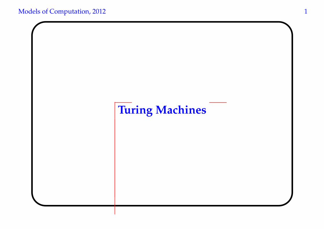
Algorithms, informally

No precise definition of “algorithm” at the time Hilbert

posed the Entscheidungsproblem, just examples.

Common features of the examples of algorithms:

• finite description of the procedure in terms of

elementary operations;

• deterministic, next step is uniquely determined if

there is one;

• procedure may not terminate on some input data,

but we can recognise when it does terminate and

what the result is.

Models of Computation, 2012 1

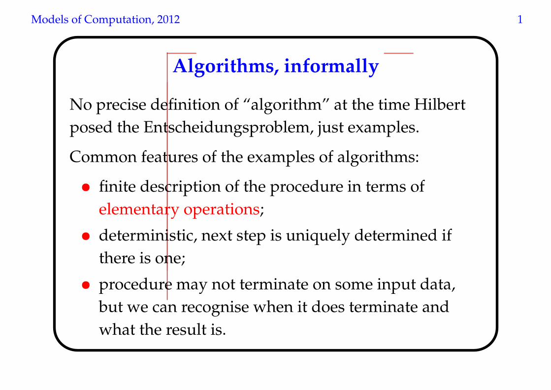
Turing machines, informally

q

↓

· · · 0 1 0 1 1 · · ·

Models of Computation, 2012 1

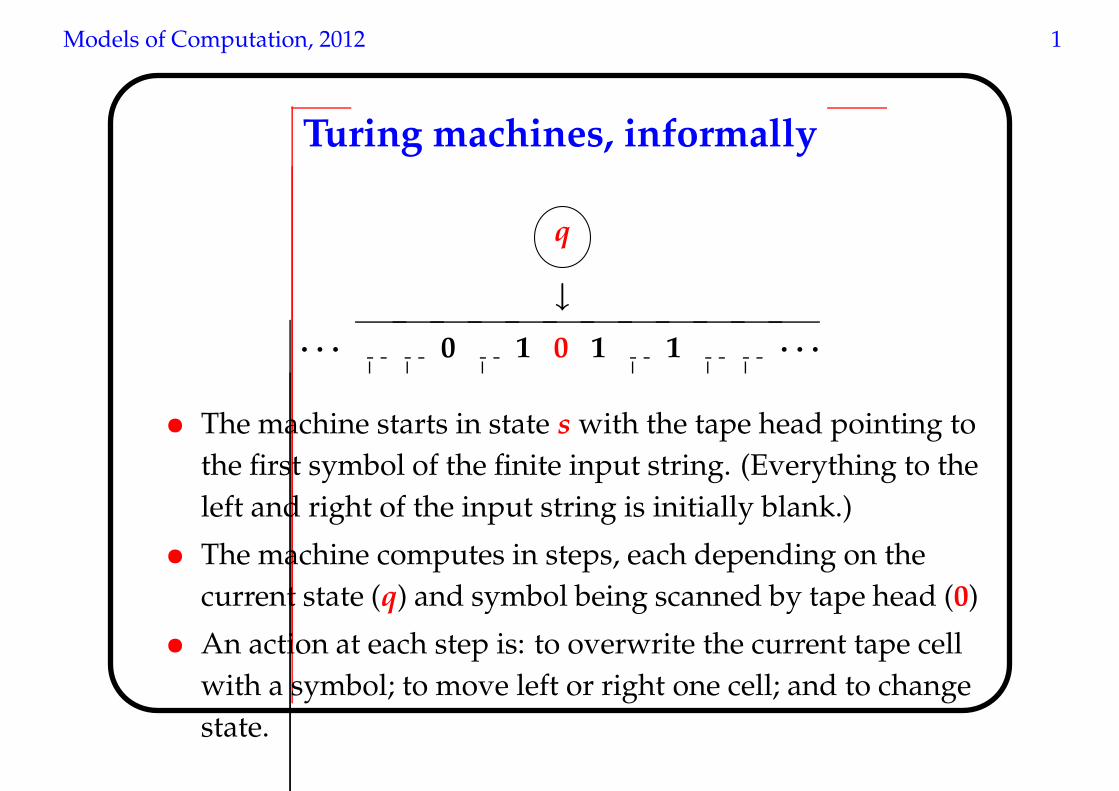
Turing machines, informally

q

↓

· · · 0 1 0 1 1 · · ·

• The machine starts in state s with the tape head pointing to

the first symbol of the finite input string. (Everything to the

left and right of the input string is initially blank.)

• The machine computes in steps, each depending on the

current state (q) and symbol being scanned by tape head (0)

• An action at each step is: to overwrite the current tape cell

with a symbol; to move left or right one cell; and to change

state.

Models of Computation, 2012 1

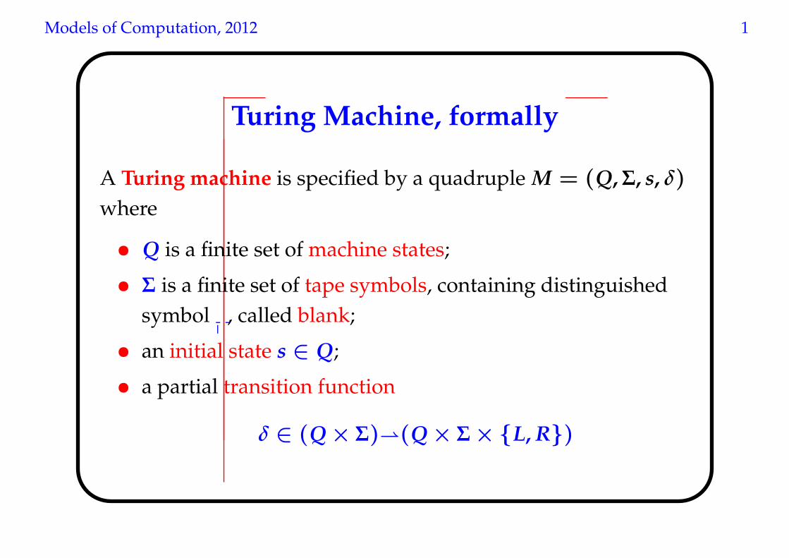
Turing Machine, formally

A Turing machine is specified by a quadruple M = (Q, Σ, s, δ)

where

• Q is a finite set of machine states;

• Σ is a finite set of tape symbols, containing distinguished

symbol , called blank;

• an initial state s ∈ Q;

• a partial transition function

δ ∈ (Q × Σ)⇀(Q × Σ × {L, R})

Models of Computation, 2012 1

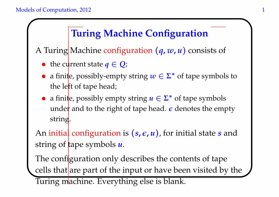
Turing Machine Configuration

A Turing Machine configuration (q, w, u) consists of

• the current state q ∈ Q;

• a finite, possibly-empty string w ∈ Σ∗ of tape symbols to

the left of tape head;

• a finite, possibly empty string u ∈ Σ∗ of tape symbols

under and to the right of tape head. ǫ denotes the empty

string.

An initial configuration is (s, ǫ, u), for initial state s and

string of tape symbols u.

The configuration only describes the contents of tape

cells that are part of the input or have been visited by the

Turing machine. Everything else is blank.

Models of Computation, 2012 1

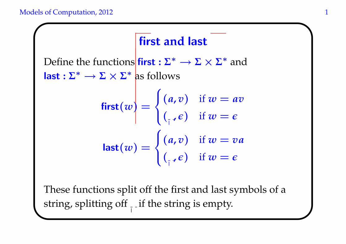
first and last

Define the functions first : Σ∗ → Σ × Σ

∗ and

last : Σ∗ → Σ × Σ

∗ as follows

first(w) =

(a, v) if w = av

( , ǫ) if w = ǫ

last(w) =

(a, v) if w = va

( , ǫ) if w = ǫ

These functions split off the first and last symbols of a

string, splitting off if the string is empty.

Models of Computation, 2012 1

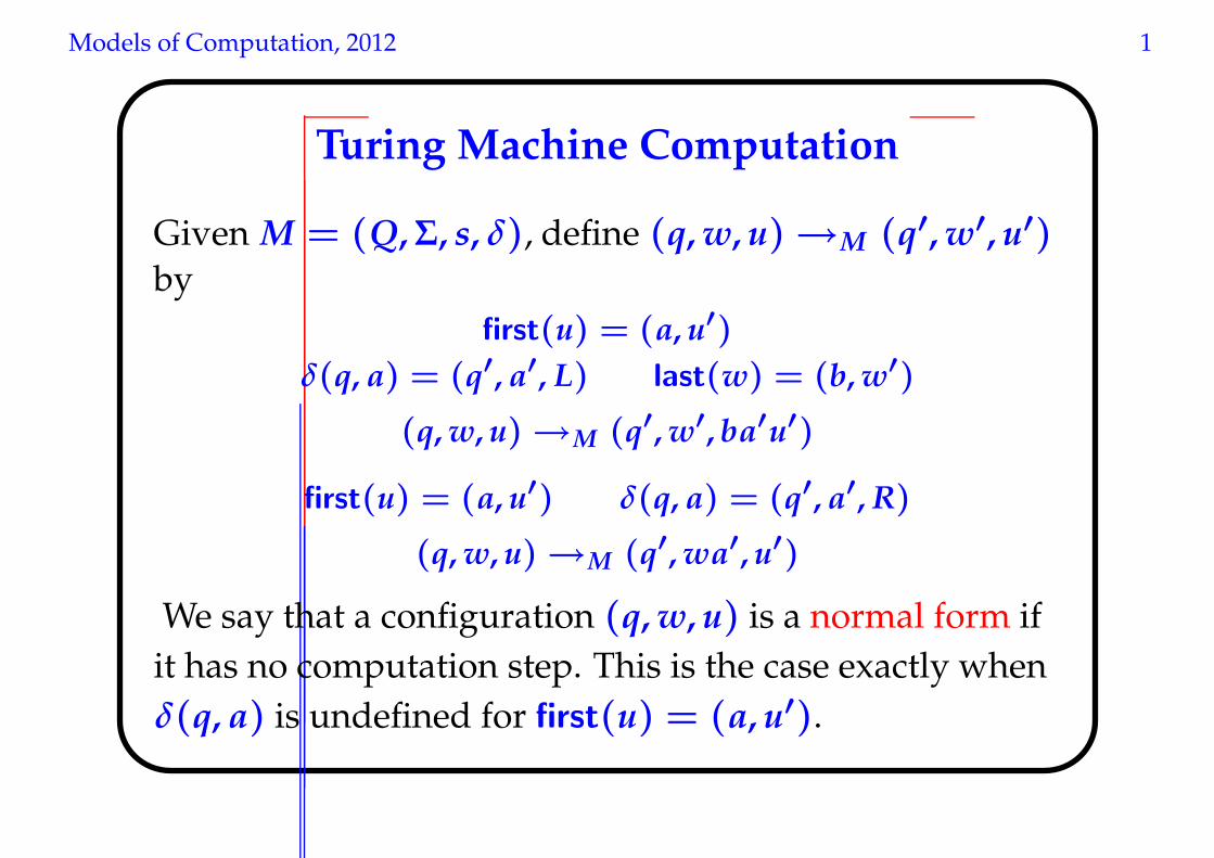
Turing Machine Computation

Given M = (Q, Σ, s, δ), define (q, w, u) →M (q′, w′, u′)by

first(u) = (a, u′)

δ(q, a) = (q′, a′, L) last(w) = (b, w′)

(q, w, u) →M (q′, w′, ba′u′)

first(u) = (a, u′) δ(q, a) = (q′, a′, R)

(q, w, u) →M (q′, wa′, u′)

We say that a configuration (q, w, u) is a normal form if

it has no computation step. This is the case exactly when

δ(q, a) is undefined for first(u) = (a, u′).

Models of Computation, 2012 1

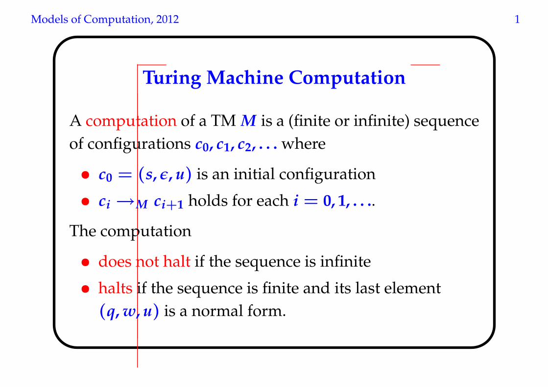
Turing Machine Computation

A computation of a TM M is a (finite or infinite) sequence

of configurations c0, c1, c2, . . . where

• c0 = (s, ǫ, u) is an initial configuration

• ci →M ci+1 holds for each i = 0, 1, . . ..

The computation

• does not halt if the sequence is infinite

• halts if the sequence is finite and its last element

(q, w, u) is a normal form.

Models of Computation, 2012 1

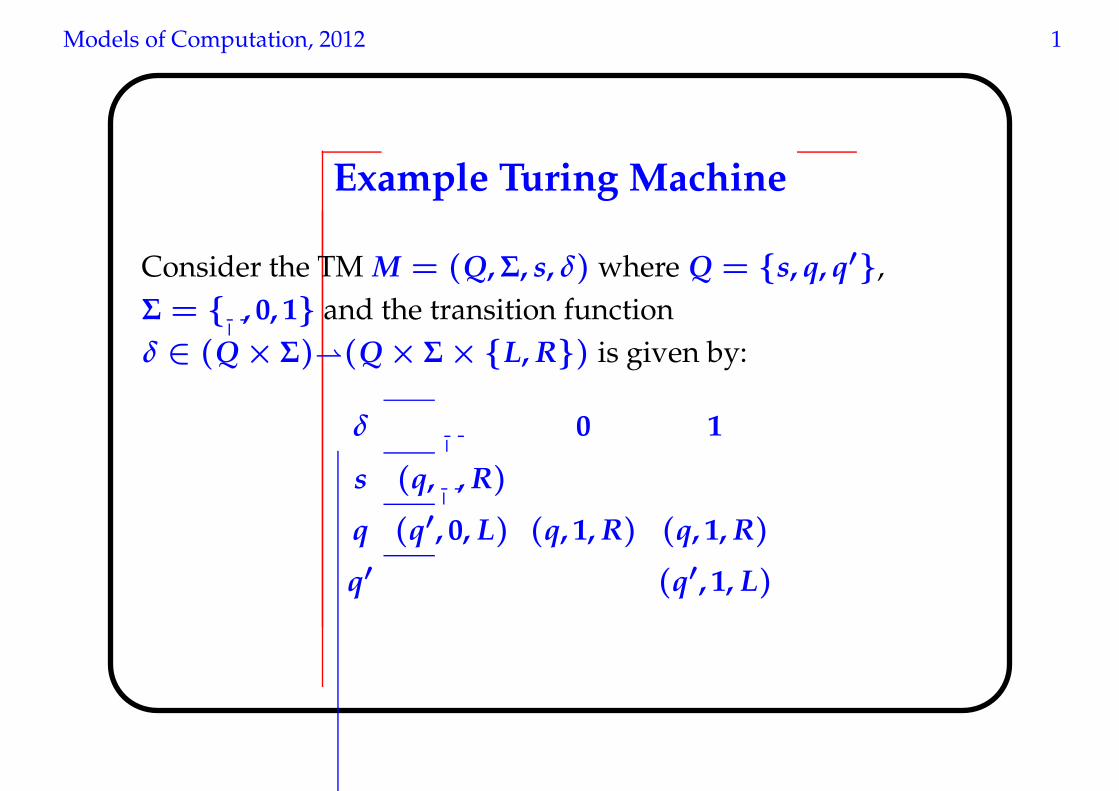
Example Turing Machine

Consider the TM M = (Q, Σ, s, δ) where Q = {s, q, q′},

Σ = { , 0, 1} and the transition function

δ ∈ (Q × Σ)⇀(Q × Σ × {L, R}) is given by:

δ 0 1

s (q, , R)

q (q′, 0, L) (q, 1, R) (q, 1, R)

q′ (q′, 1, L)

Models of Computation, 2012 1

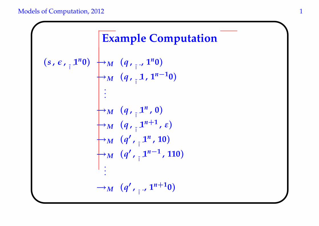
Example Computation

(s , ǫ , 1n0) →M (q , , 1n0)

→M (q , 1 , 1n−10)...

→M (q , 1n , 0)

→M (q , 1n+1 , ε)

→M (q′ , 1n , 10)

→M (q′ , 1n−1 , 110)...

→M (q′ , , 1n+10)

Models of Computation, 2012 1

Theorem. The computation of a Turing machine M can

be implemented by a register machine.

Proof (sketch).

Step 1: fix a numerical encoding of M’s states, tape

symbols, tape contents and configurations.

Step 2: implement M’s transition function (finite table)

using RM instructions on codes.

Step 3: implement a RM program to repeatedly carry out

→M .

Models of Computation, 2012 1

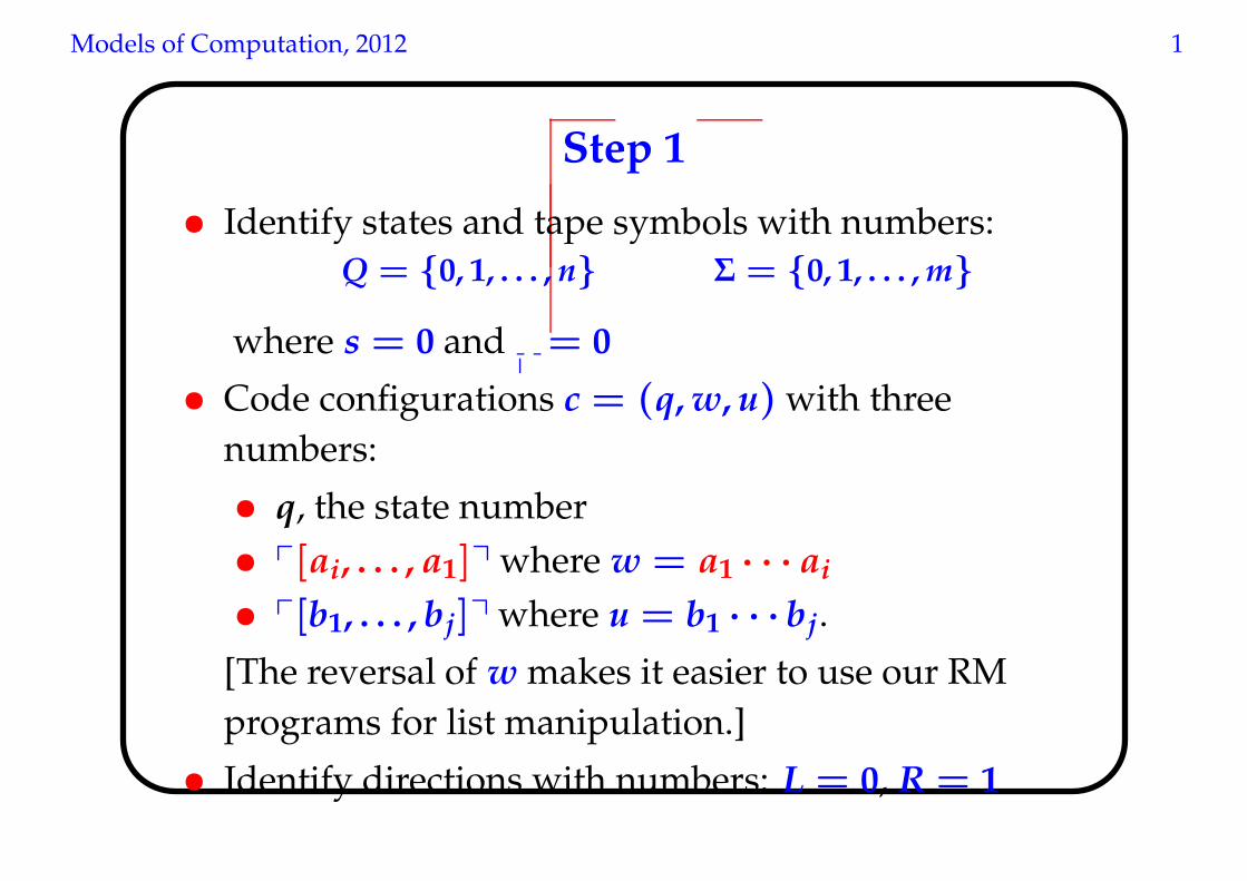
Step 1

• Identify states and tape symbols with numbers:

Q = {0, 1, . . . , n} Σ = {0, 1, . . . , m}

where s = 0 and = 0

• Code configurations c = (q, w, u) with three

numbers:

• q, the state number

• p[ai, . . . , a1]q where w = a1 · · · ai

• p[b1, . . . , bj]q where u = b1 · · · bj.

[The reversal of w makes it easier to use our RM

programs for list manipulation.]

• Identify directions with numbers: L = 0, R = 1

Models of Computation, 2012 1

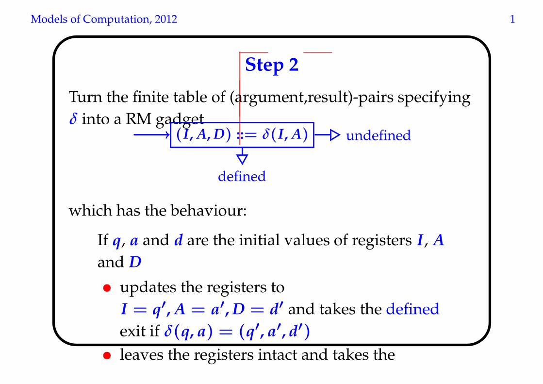
Step 2

Turn the finite table of (argument,result)-pairs specifying

δ into a RM gadget(I, A, D) ::= δ(I, A)

defined

undefined

which has the behaviour:

If q, a and d are the initial values of registers I, A

and D

• updates the registers to

I = q′, A = a′, D = d′ and takes the defined

exit if δ(q, a) = (q′, a′, d′)

• leaves the registers intact and takes the

Models of Computation, 2012 1

undefined exit if δ(q, a) is undefined

Models of Computation, 2012 1

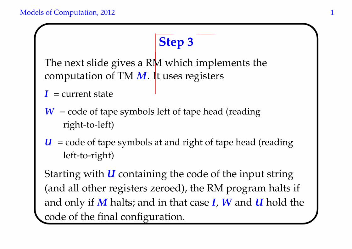
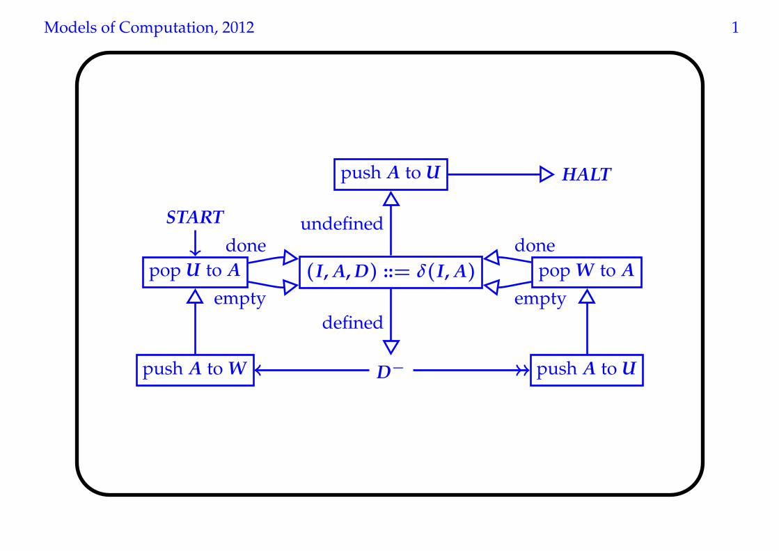
Step 3

The next slide gives a RM which implements thecomputation of TM M. It uses registers

I = current state

W = code of tape symbols left of tape head (reading

right-to-left)

U = code of tape symbols at and right of tape head (reading

left-to-right)

Starting with U containing the code of the input string

(and all other registers zeroed), the RM program halts if

and only if M halts; and in that case I, W and U hold the

code of the final configuration.

Models of Computation, 2012 1

pop U to A

START

(I, A, D) ::= δ(I, A)

push A to U HALT

D−push A to W push A to U

pop W to A

done

empty

undefined

defined

done

empty

Models of Computation, 2012 1

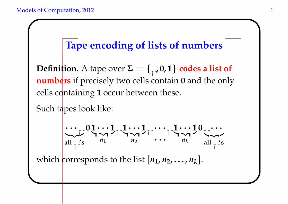
Tape encoding of lists of numbers

Definition. A tape over Σ = { , 0, 1} codes a list of

numbers if precisely two cells contain 0 and the only

cells containing 1 occur between these.

Such tapes look like:

· · ·︸ ︷︷ ︸

all ′s

0 1 · · · 1︸ ︷︷ ︸

n1

1 · · · 1︸ ︷︷ ︸

n2 · · ·

· · · 1 · · · 1︸ ︷︷ ︸

nk

0 · · ·︸ ︷︷ ︸

all ′s

which corresponds to the list [n1, n2, . . . , nk].

Models of Computation, 2012 1

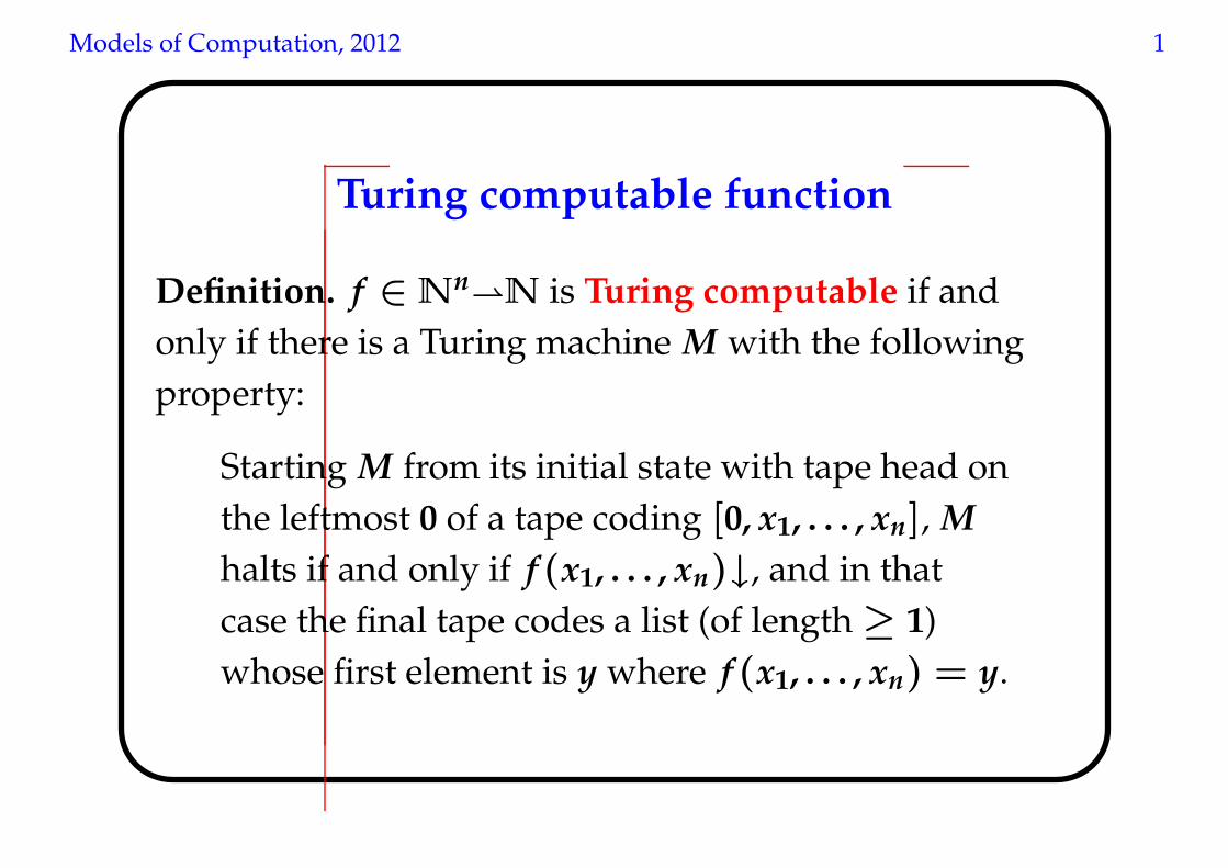
Turing computable function

Definition. f ∈ Nn⇀N is Turing computable if and

only if there is a Turing machine M with the following

property:

Starting M from its initial state with tape head on

the leftmost 0 of a tape coding [0, x1, . . . , xn], M

halts if and only if f (x1, . . . , xn)↓, and in that

case the final tape codes a list (of length ≥ 1)

whose first element is y where f (x1, . . . , xn) = y.

Models of Computation, 2012 1

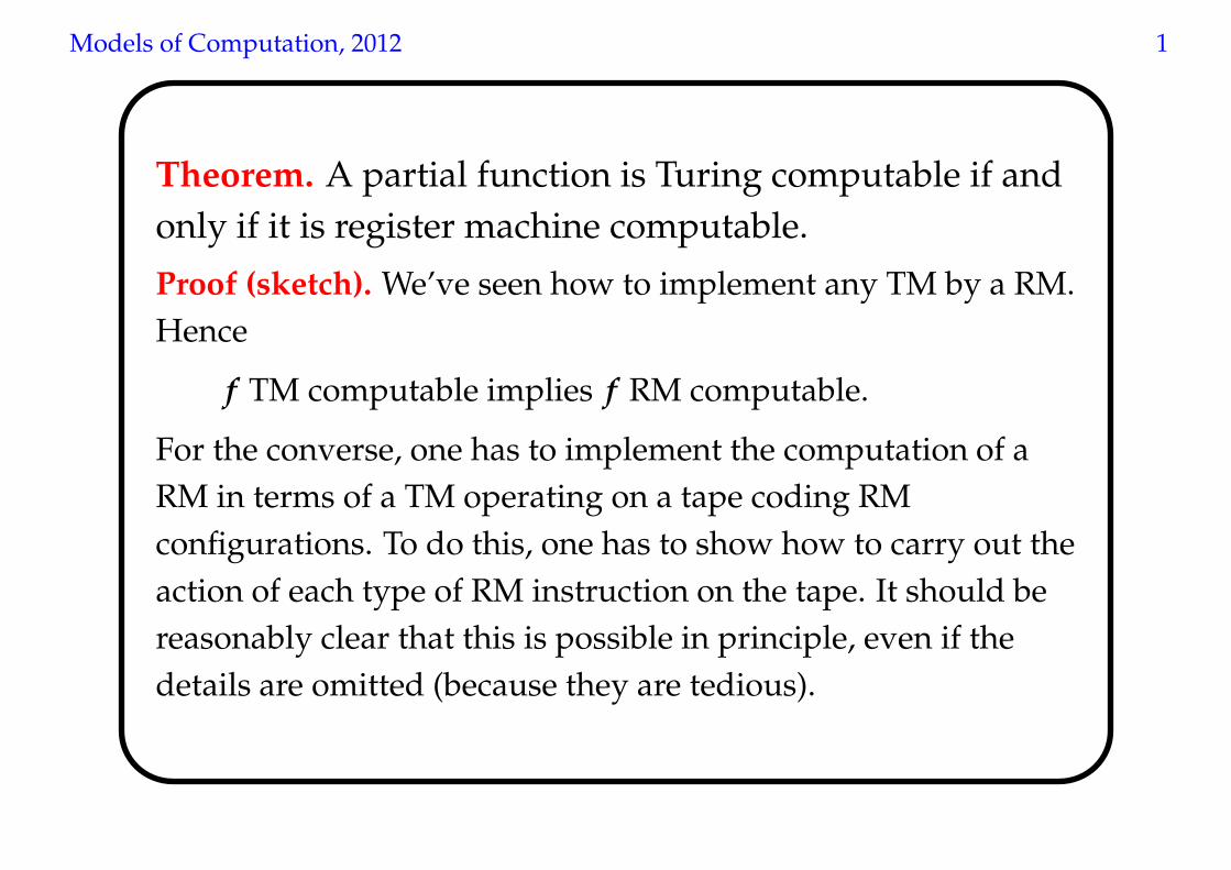
Theorem. A partial function is Turing computable if and

only if it is register machine computable.

Proof (sketch). We’ve seen how to implement any TM by a RM.

Hence

f TM computable implies f RM computable.

For the converse, one has to implement the computation of a

RM in terms of a TM operating on a tape coding RM

configurations. To do this, one has to show how to carry out the

action of each type of RM instruction on the tape. It should be

reasonably clear that this is possible in principle, even if the

details are omitted (because they are tedious).

Models of Computation, 2012 1

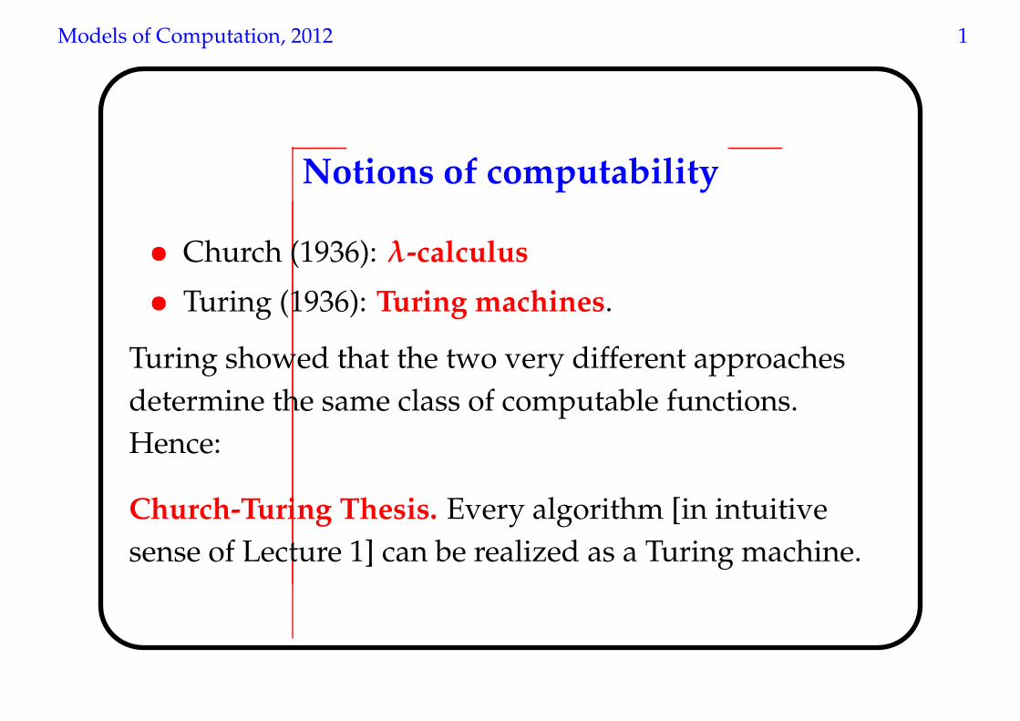
Notions of computability

• Church (1936): λ-calculus

• Turing (1936): Turing machines.

Turing showed that the two very different approaches

determine the same class of computable functions.

Hence:

Church-Turing Thesis. Every algorithm [in intuitive

sense of Lecture 1] can be realized as a Turing machine.

Models of Computation, 2012 1

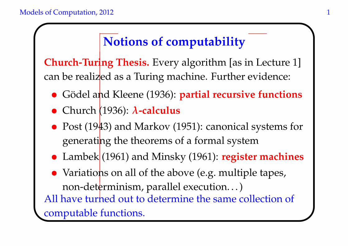
Notions of computability

Church-Turing Thesis. Every algorithm [as in Lecture 1]

can be realized as a Turing machine. Further evidence:

• Gödel and Kleene (1936): partial recursive functions

• Church (1936): λ-calculus

• Post (1943) and Markov (1951): canonical systems for

generating the theorems of a formal system

• Lambek (1961) and Minsky (1961): register machines

• Variations on all of the above (e.g. multiple tapes,

non-determinism, parallel execution. . . )All have turned out to determine the same collection of

computable functions.