Turbulence Observations Above a Smooth Melting Surface on the Greenland Ice Sheet

TURBULENCE OBSERVATIONS ABOVE A SMOOTH MELTINGSURFACE ON THE GREENLAND ICE SHEET

A. G. C. A. MEESTERS, N. J. BINK, H. F. VUGTS, F. CANNEMEIJER andE. A. C. HENNEKEN

Institute of Earth Sciences, Vrije Universiteit, De Boelelaan 1085, 1081 HV Amsterdam, TheNetherlands

(Received in final form 21 April, 1997)

Abstract. Measurements of profiles and turbulent fluxes have been made over a smooth, meltingsurface on the southwestern part of the Greenland ice sheet in July 1991. For a reference height of0.8 m, and flux measurements at 4 m and 13 m, the best values for the roughness lengths are 3�10�4 m for wind speed, 2� 10�6 m for temperature, and 5� 10�4 m for moisture. The uncertaintyin the corresponding exchange coefficients is about 10%. The roughness length for temperature (zT )is much smaller than expected from theory, as was also found in a number of earlier investigations.The possibility is considered that absorption of shortwave radiation by aerosol particles accumulatingnear the surface lowers the zT values. Consequently, zT using lower measurement heights shouldprobably be close to z0. However, evidence for this remains rather indirect. Further, it is shown thatreliable results for the sensible heat flux can be obtained using the product of the observed standarddeviation for temperature fluctuations and wind speed.

Key words: Polar meteorology, Snow and ice surfaces, Roughness length for temperature, Radiationabsorption

1. Introduction

Much interest has arisen recently in the response of the Greenland ice sheet toclimate change. For the investigation of this response, reliable parameterizationsof the surface exchange of momentum, heat and moisture are required. Of specialimportance is the ablation zone of the ice sheet, where the yearly meltwater pro-duction exceeds the yearly snow- and rainfall. The determination of the melt rate inthe ablation zone is important for the prediction of sea-level rise. Apart from this,the melting conditions in summer are attractive for boundary-layer research sincethey offer the opportunity to perform investigations over a vast homogeneous areawhere the surface temperature is accurately known. On the other hand, the meltingconditions cause a number of notorious problems for carrying out measurements(Oerlemans and Vugts, 1993), and observations in this area have long remainedscarce for this reason.

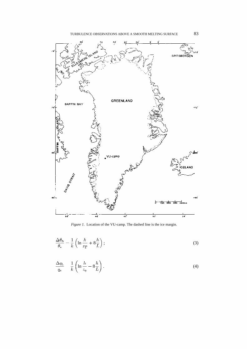
The observations to be discussed in this paper were performed in July 1991 atthe upper boundary of the ablation area on the southwestern part of the Greenlandice sheet. The location (Figure 1) is close to the polar circle, at a distance of 90 kmfrom the ice margin (67�020 N, 48�120 W, about 1500 m a.s.l.). The measurementstation was operated by the Institute for Earth Sciences of the Vrije UniversiteitAmsterdam (VU), and will be referred to as the VU-camp. The observations were

Boundary-Layer Meteorology 85: 81–110, 1997.c 1997 Kluwer Academic Publishers. Printed in the Netherlands.

82 A. G. C. A. MEESTERS ET AL.

part of the Greenland Ice Margin Experiment (GIMEX), in which the Institute ofMarine and Atmospheric Research of the University of Utrecht (IMAU) operateda number of other stations, all of which were located at the same latitude but ata smaller distance from the west coast. Three of these stations were located onthe ice, whereas others were located in the broad ice-free region between the icesheet and the sea. Oerlemans and Vugts (1993) and Van den Broeke et al. (1994)presented the purpose and experimental set-up of the GIMEX project and the majorclimatological results, including those for the VU-camp. Other meteorologicalGIMEX publications show the enhancement of ice melt by the presence of theice-free zone, and contribute to understanding the complicated atmosphere-iceinteraction in this region and its sensitivity to climate change (Meesters, 1994;Gallee et al., 1995; Van den Broeke and Gallee, 1996; Van de Wal et al., 1995).

Of special importance for the present paper is the work that has been done ondetermining fluxes and roughness lengths z0 for wind speed, zT for temperatureand zq for humidity from profile observations. Duynkerke and Van den Broeke(1994) calculated turbulent fluxes from profile data only, for the GIMEX stations,including the VU-camp. For the VU-camp, the calculated heat fluxes appear tobe twice as high as the directly measured values that are given by Henneken etal. (1994, 1997). Contributions to this discrepancy may include the inaccuracy ofthe temperature measurements (for which the profile method is very sensitive), thelimited boundary-layer height, and the doubtful assumption zT = z0 which wasused in the calculation. Because of these difficulties, methods relying on verticalgradients will be avoided in this paper. We add for completeness that for the otherGIMEX sites on the ice, the results of the profile method (Duynkerke and Van denBroeke, 1994) had to be revised for another reason, namely the hilliness of thesurface at those sites (Van den Broeke, 1996, Chapter 5).

In this paper, emphasis will be on the bulk method. For heat, for which thereare problems with the bulk method as will be seen, the standard deviation methodwill also be considered.

2. Theory

Most of the formalism used in this paper is standard so that only specific assump-tions have to be listed here. The fluxes of momentum (� ), sensible heat (H) andlatent heat (�E) are related to u

�, �

�and q

�by

� = �u2�

; H = ��cpu��; �E = ��u�q�; (1)

in which � = 1.1 kg m�3, cp = 1005 J kg�1 K�1 and � = 2.501 � 106 J kg�1. Thefollowing flux-profile relations are assumed as ‘standard relations’ for the surfacelayer (Hogstrom, 1988, but with rounded-off coefficients):

vhu�

=1k

�ln

h

z0+ 6

h

L

�; (2)

TURBULENCE OBSERVATIONS ABOVE A SMOOTH MELTING SURFACE 83

Figure 1. Location of the VU-camp. The dashed line is the ice margin.

��h��

=1k

�ln

h

zT+ 8

h

L

�; (3)

�qhq�

=1k

ln

h

zq+ 8

h

L

!: (4)


in which ��h = �h � �0 and �qh = qh � q0, k = 0.4, and L = (�0=kg)u2�

=��

is the Obukhov length (g = 9.8 m s�2). For the cases considered in this paper thesurface is always at the melting point, hence �0 = 0 �C = 273.15 K. The transfercoefficients CD = u2

�

=v2h, CH = u

��=(vh��h) and CE = u

�q�=(vh�qh) will

only be used for a small reference height h (0.8 m) and weakly stable cases, sothat the stability corrections are small (see Section 4.2, first paragraph). Neglectingthese corrections yields

CD =k2�

lnh

z0

�2 ; CH =k2

lnh

z0ln

h

zT

; CE =k2

lnh

z0ln

h

zq

: (5)

The validity of the Equations (2)–(4) can be disturbed by non-stationarity (whichwill be reduced by the selection of the time intervals), by entrainment (at the topof the boundary layer), by radiative flux divergence, and by advection. The lattertwo effects will be discussed in Section 4.3.

3. Site and Instrumentation

The position of the VU-camp has been given in the introduction. On a large scale,the terrain slopes down to the west, with a slope angle of about 0.01 radian. Localgeodetic measurements indicate that the same holds on a local scale. The windwas from the SE, with a high directional constancy of 0.94 (Van den Broeke et al.,1994). It was shown by numerical simulation by Meesters et al. (1994) that the SEdirection is caused by the deflection of the katabatic wind by the Coriolis force. Thedata presented in this paper were obtained between 4 and 23 July 1991. The nightswere very short or (at the beginning) absent. The surface was almost continuouslyat, or close to, the melting point. Due to the high temperatures, there were only fewproblems with the instruments caused by freezing or snowdrift. At the start of theexperiment, the ice was covered with a snow layer which transformed into slush.At about 14 July the snow had disappeared to a great extent, and from that date theice surface changed locally into fields of large ice crystals with a diameter of about2 cm and a length of about 7 cm.

Profile measurements have been performed along a 31 m high tower. Duringthe period of the observations, the ice surface was lowered by about 0.4 m dueto melting, so that the relative heights of the instruments were rising. The heightsgiven in the following are averages over the period. The wind speed was measuredwith home-made cup anemometers at 8 levels (namely at 0.8, 1.1, 1.6, 2.6, 4, 8, 16and 30 m above the surface). The wind direction was measured with wind vanes at2 m and at 31 m. The temperatures were measured using Rotronic sensors, placedat 6 heights (0.8, 1.6, 2.6, 4, 8, and 30 m). Since the sensors were not aspirated,the temperatures required rather large corrections for radiation errors. These were


performed as follows. During the whole expedition, the temperature readings ofone of the sensors and of an Assman aspirated psychrometer were compared, andthe difference was explained in terms of radiation and wind speed by multivariatelinear regression. The other sensors were calibrated by intercomparison carriedout at the same location with the instruments hung at the same height during oneday. The calibrated 1.6 m temperatures still showed unexplained deviations andhad to be dismissed. The error in the calibrated temperatures is assumed to be 0.2to 0.3 K. Relative humidities were also measured with the Rotronic sensors. Theabsolute humidities are calculated from the relative humidities and the instrumenttemperatures, so they do not suffer from the problems with the air temperatures.The humidity record of one level (2.6 m) was dismissed, however, as it showedunexplained deviations. The other humidities were calibrated by requiring thatthe humidity was 100% under fog conditions. Afterwards, they required constantcorrections of at most 1% (which typically corresponds to an error of 0.05 g kg�1

in the mixing ratio).To determine the surface temperature, the outgoing longwave radiation was

measured. However, the quality of these measurements was poor, as appeared fromthe large scatter (even after correction for the reflected radiation) under conditionswith melting when the radiation should be constant. These measurements havebeen discarded for this paper.

For the measurement of turbulent fluxes, eddy correlation systems were em-ployed at heights of 4 m and 13 m. Each system consisted of a Solent 3-axis sonicanemometer (path length 15 cm), a Lyman-� humidity fluctuation sensor (GlassTechnologists) with a source-detector distance of 1.5 cm, and a thermocouple.The sample frequency was 20 Hz. Each sonic was placed on a slender extensionon top of a mast. To minimize the distortion of the flow through the sonic, thethermocouple and the Lyman-� were located downwind of the sonic anemometer.The distance between the microphones of the sonics was measured with an accuracyof 1 mm. The sonic anemometer was put as level as possible (within �1�). Thiswas checked on a regular basis. The fluxes were corrected for the terrain slopeas well as for flow distortion by rotating the fluctuating wind vector around ahorizontal axis perpendicular to the wind direction so that the mean of the verticalwind became zero. The mean rotation angle was �0.012 radian, in good accordwith the estimated terrain slope (�0.01).

The thermocouples missed a reflective coating so that they absorbed much(direct and reflected) solar radiation. Hence a spurious covariance of w0 and �0 wasgenerated, which was estimated following Jacobs and McNaughton (1994) andwhich appears to be so high compared to the true w0�0 (which was small) that thethermocouple data had to be discarded. They were replaced by sonic temperatures.

The observations were corrected for high frequency loss due to sensor separationand limited time response according to Raupach (1977). The random errors in theobserved fluxes (half-hour means) have been calculated according to the methoddescribed in Kaimal and Finnigan (1994). Due to the smallness of the scalar fluxes,


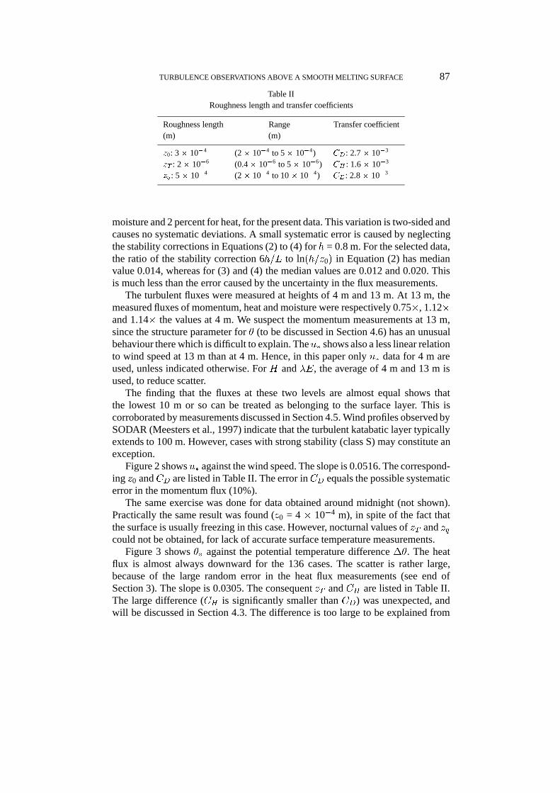
Table IClassification of the observed half-hour cases

Acronym Name Definition Number of cases

N Neutral v8 < 6 m s�1, RiB8 � 0.03 42S Stable v8 < 6 m s�1, RiB8 > 0.03 37WN Windy neutral v8 � 6 m s�1, RiB8 � 0.02 42WS Windy stable v8 � 6 m s�1, RiB8 > 0.02 15

these errors can be large (up to 50%). However, because of the large number (136)of cases the consequent random errors in the calculated slope coefficients (Section4.2) are below 5% (even smaller for momentum). However, there are also smallsystematic errors remaining despite the applied corrections, and it is estimated thatthe possible systematic error in the flux measurements amounts to 10% for thisreason.

4. Results

4.1. SELECTION AND CLASSIFICATION OF THE CASES

For performing bulk calculations, the surface temperature should be known. Sinceradiative temperature measurements appeared not accurate enough for this purpose,we restrict ourselves to cases for which the surface was at the melting point. Further,only cases between 1100 and 1730 hr local time (= UT � 3 hr) are considered,so that the disturbance of the flux measurements by non-stationarity is in generalsmall (precisely, the lowest sensor recorded for 94 percent of the cases a j@�=@tjnot exceeding the equivalent of 0.10 W m�3 flux divergence, moreover the average@�=@t is practically zero, and for moisture the equivalent of 0.10 W m�3 was onlyexceeded for one case). In the end, 136 useful half hour periods with melting surface(and without snowdrift) remained. These periods were classified according to the8 m wind speed v8 and the 8 m bulk Richardson number RiB8. The classificationis shown in Table I. The division is such that the individual profiles of temperatureand wind within each class are as similar as possible.

4.2. DETERMINATION OF TRANSFER COEFFICIENTS AND ROUGHNESS LENGTHS

To determine transfer coefficients, the wind, temperature and moisture data fromthe lowest sensors were used to avoid difficulties caused by lack of adjustmentof the air flow to the surface. In calculating roughness lengths from ln(h=z0),ln(h=zT ) and ln(h=zq), it is assumed that h = 0.8 m, though this is only an averagevalue (as the surface lowered by melting). The change of h around its mean causesa deviation of ln(h=z0) which amounts to at most 3.5 percent for momentum and


Table IIRoughness length and transfer coefficients

Roughness length Range Transfer coefficient(m) (m)

z0: 3 � 10�4 (2 � 10�4 to 5 � 10�4) CD: 2.7 � 10�3

zT : 2 � 10�6 (0.4 � 10�6 to 5 � 10�6) CH : 1.6 � 10�3

zq: 5 � 10�4 (2 � 10�4 to 10 � 10�4) CE : 2.8 � 10�3

moisture and 2 percent for heat, for the present data. This variation is two-sided andcauses no systematic deviations. A small systematic error is caused by neglectingthe stability corrections in Equations (2) to (4) for h = 0.8 m. For the selected data,the ratio of the stability correction 6h=L to ln(h=z0) in Equation (2) has medianvalue 0.014, whereas for (3) and (4) the median values are 0.012 and 0.020. Thisis much less than the error caused by the uncertainty in the flux measurements.

The turbulent fluxes were measured at heights of 4 m and 13 m. At 13 m, themeasured fluxes of momentum, heat and moisture were respectively 0.75�, 1.12�and 1.14� the values at 4 m. We suspect the momentum measurements at 13 m,since the structure parameter for � (to be discussed in Section 4.6) has an unusualbehaviour there which is difficult to explain. Theu

�shows also a less linear relation

to wind speed at 13 m than at 4 m. Hence, in this paper only u�

data for 4 m areused, unless indicated otherwise. For H and �E, the average of 4 m and 13 m isused, to reduce scatter.

The finding that the fluxes at these two levels are almost equal shows thatthe lowest 10 m or so can be treated as belonging to the surface layer. This iscorroborated by measurements discussed in Section 4.5. Wind profiles observed bySODAR (Meesters et al., 1997) indicate that the turbulent katabatic layer typicallyextends to 100 m. However, cases with strong stability (class S) may constitute anexception.

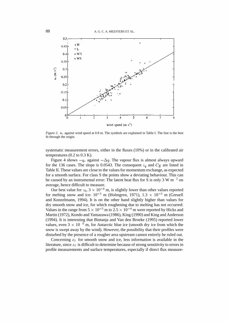
Figure 2 shows u�

against the wind speed. The slope is 0.0516. The correspond-ing z0 and CD are listed in Table II. The error inCD equals the possible systematicerror in the momentum flux (10%).

The same exercise was done for data obtained around midnight (not shown).Practically the same result was found (z0 = 4 � 10�4 m), in spite of the fact thatthe surface is usually freezing in this case. However, nocturnal values of zT and zqcould not be obtained, for lack of accurate surface temperature measurements.

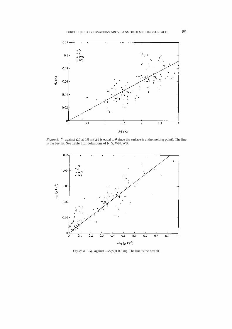
Figure 3 shows ��

against the potential temperature difference ��. The heatflux is almost always downward for the 136 cases. The scatter is rather large,because of the large random error in the heat flux measurements (see end ofSection 3). The slope is 0.0305. The consequent zT and CH are listed in Table II.The large difference (CH is significantly smaller than CD) was unexpected, andwill be discussed in Section 4.3. The difference is too large to be explained from


Figure 2. u� against wind speed at 0.8 m. The symbols are explained in Table I. The line is the bestfit through the origin.

systematic measurement errors, either in the fluxes (10%) or in the calibrated airtemperatures (0.2 to 0.3 K).

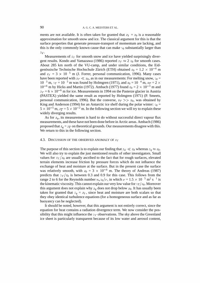
Figure 4 shows �q�

against ��q. The vapour flux is almost always upwardfor the 136 cases. The slope is 0.0543. The consequent zq and CE are listed inTable II. These values are close to the values for momentum exchange, as expectedfor a smooth surface. For class S the points show a deviating behaviour. This canbe caused by an instrumental error: The latent heat flux for S is only 3 W m�2 onaverage, hence difficult to measure.

Our best value for z0, 3 � 10�4 m, is slightly lower than other values reportedfor melting snow and ice: 10�3 m (Holmgren, 1971), 1.3 � 10�3 m (Greuelland Konzelmann, 1994). It is on the other hand slightly higher than values fordry smooth snow and ice, for which roughening due to melting has not occurred:Values in the range from 5� 10�5 m to 2.5� 10�4 m were reported by Hicks andMartin (1972), Kondo and Yamazawa (1986), King (1990) and King and Anderson(1994). It is interesting that Bintanja and Van den Broeke (1995) reported lowervalues, even 3 � 10�6 m, for Antarctic blue ice (smooth dry ice from which thesnow is swept away by the wind). However, the possibility that their profiles weredisturbed by the presence of a rougher area upstream cannot entirely be ruled out.

Concerning zT for smooth snow and ice, less information is available in theliterature, since zT is difficult to determine because of strong sensitivity to errors inprofile measurements and surface temperatures, especially if direct flux measure-


Figure 3. �� against �� at 0.8 m (�� is equal to � since the surface is at the melting point). The lineis the best fit. See Table I for definitions of N, S, WN, WS.

Figure 4. �q� against ��q (at 0.8 m). The line is the best fit.


ments are not available. It is often taken for granted that zT = z0 is a reasonableapproximation for smooth snow and ice. The classical argument for this is that thesurface properties that generate pressure-transport of momentum are lacking, andthis is the only commonly known cause that can make z0 substantially larger thanzT .

Measurements of zT for smooth snow and ice have yielded surprisingly diver-gent results. Kondo and Yamazawa (1986) reported zT � 2 z0 for smooth cases.About 285 km north of the VU-camp, and under similar conditions, the Eid-genossische Technische Hochschule Zurich (ETH) obtained z0 = 1.2 � 10�4 mand zT = 3 � 10�5 m (J. Forrer, personal communication, 1996). Many caseshave been reported with zT � z0, as in our measurements: For melting snow, z0 =10�3 m, zT = 10�5 m was found by Holmgren (1971), and z0 = 10�4 m, zT = 2 �10�6 m by Hicks and Martin (1972). Ambach (1977) found z0 = 2 � 10�3 m andzT = 6� 10�6 m for ice. Measurements in 1994 on the Pasterze glacier in Austria(PASTEX) yielded the same result as reported by Holmgren (1971) (P. Smeets,personal communication, 1996). But the converse, zT >> z0, was obtained byKing and Anderson (1994) for an Antarctic ice shelf during the polar winter: z0 =5� 10�5 m, zT = 5� 10�2 m. In the following section we will try to explain thesewidely diverging results.

As for zq , its measurement is hard to do without successful direct vapour fluxmeasurements, and these have not been done before in Arctic areas. Ambach (1986)proposed that zq = zT on theoretical grounds. Our measurements disagree with this.We return to this in the following section.

4.3. DISCUSSION OF THE OBSERVED ANOMALY OF zT

The purpose of this section is to explain our finding that zT � z0 whereas zq � z0.We will also try to explain the just mentioned results of other investigators. Smallvalues for zT =z0 are usually ascribed to the fact that for rough surfaces, elevatedterrain elements increase friction by pressure forces which do not influence theexchange of heat and moisture at the surface. But in the present case the surfacewas relatively smooth, with z0 = 3 � 10�4 m. The theory of Andreas (1987)predicts that zT =z0 is between 0.3 and 0.9 for this case. This follows from therange 2 to 6 for the Reynolds number u

�z0=�, in which � = 1.5 � 10�5 m2 s�1 is

the kinematic viscosity. This cannot explain our very low value for zT=z0. Moreoverthis argument does not explain why zq does not drop below z0. It has usually beentaken for granted that zq = zT , since heat and moisture are both scalars so thatthey obey identical turbulence equations (for a homogeneous surface and as far asbuoyancy can be neglected).

It should be noted, however, that this argument is not entirely correct, since theequation for heat contains a radiation divergence term. We now consider the pos-sibility that this might influence the zT observations. The sky above the Greenlandice sheet is particularly transparent because of its low water and aerosol content,


causing intense insolation (including much reflected insolation, the albedo is about0.7 at the VU-camp), whereas these conditions on the other hand promote diver-gence of longwave radiation. Further, the turbulent heat flux is low, typically 15W m�2 (Section 4.7), which enhances the relative importance of radiative effects.

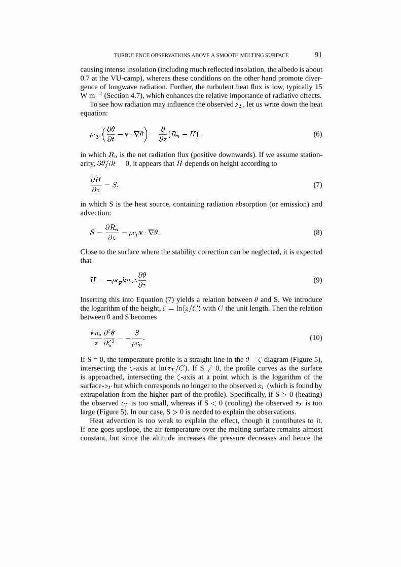
To see how radiation may influence the observed zT , let us write down the heatequation:

�cp

�@�

@t+ v � r�

�=

@

@z(Rn �H); (6)

in which Rn is the net radiation flux (positive downwards). If we assume station-arity, @�=@t = 0, it appears that H depends on height according to

@H

@z= S; (7)

in which S is the heat source, containing radiation absorption (or emission) andadvection:

S =@Rn

@z� �cpv � r�: (8)

Close to the surface where the stability correction can be neglected, it is expectedthat

H = ��cpku�z@�

@z: (9)

Inserting this into Equation (7) yields a relation between � and S. We introducethe logarithm of the height, � = ln(z=C) with C the unit length. Then the relationbetween � and S becomes

ku�

z

@2�

@�2 = �S

�cp: (10)

If S = 0, the temperature profile is a straight line in the � � � diagram (Figure 5),intersecting the �-axis at ln(zT =C). If S 6= 0, the profile curves as the surfaceis approached, intersecting the �-axis at a point which is the logarithm of thesurface-zT but which corresponds no longer to the observed zT (which is found byextrapolation from the higher part of the profile). Specifically, if S > 0 (heating)the observed zT is too small, whereas if S < 0 (cooling) the observed zT is toolarge (Figure 5). In our case, S > 0 is needed to explain the observations.

Heat advection is too weak to explain the effect, though it contributes to it.If one goes upslope, the air temperature over the melting surface remains almostconstant, but since the altitude increases the pressure decreases and hence the


Figure 5. Idealized �� ln(z) diagram, for different signs of the heating term S (see Equations (6–7)).

potential temperature increases. It can be deduced from this that the heat advectionterm is (Meesters et al., 1994):

��cpv � r� ' �cp�adu�; (11)

in which�ad = 10�2 K m�1 is the adiabatic lapse rate,u is the downslope componentof the wind, and � = 10�2 radian is the slope angle. For the present experiment, u= 3 m s�1 on average, yielding an advective term of + 0.3 W m�3.

It is unlikely that longwave radiation does supply heat. The relevant conditions(relatively moist surface layer under a clear dry sky) are similar to those above‘ordinary’ terrains during clear nights, and promote divergence rather than conver-gence of longwave radiation. This is known from temperature profiles observedduring still clear nights (Oke, 1970) as well as from computation (Garratt and Brost,1981). King and Anderson (1994) reported cases during the polar night in Antarc-tica with strong cooling of the air, which was attributed to radiation divergence.They also showed that this caused zT to become much larger than z0.

This prompts us to consider the possibility that absorption of shortwave radiationheats the air close to the surface. This seems odd at first hearing as the surface airwas clean for the cases involved. Direct measurement of radiation convergence inthe surface layer is very difficult in practice. Indirect measurement by observingthe heating rate @�=@t only makes sense at very low wind speed (and in the absenceof convection), since otherwise the developed heat is carried away by divergenceof the turbulent heat flux. Such conditions are hardly ever met above polar ice.However, there exists observational evidence for the occurrence of high heatingrates under favourable conditions in other regions.


Halberstam and Schieldge (1981) observed remarkable temperature anomaliesin warm air above melting snow in the Sierra Nevada (California, U.S.A.), at analtitude of 2100 m. Conditions were in some respects similar to ours. Incomingand reflected insolation were strong. But contrary to our case, the typical windspeed was only 1 m s�1, so that the influence of radiation on the profile was notmasked by turbulence. A maximum in the temperature was observed somewhatbelow 1 m. There, the temperature could become 14 �C which was several degreeswarmer than the temperature at 2 m. Anomalous profiles of the same type wereobserved over melting snow by De la Casiniere (1974), and by Granger (1977) assummarized in Male and Granger (1981).

To explain such results, a strong radiation absorption is required. From the timeseries of temperature in Halberstam and Schieldge (1981), a peak value above 1.0W m�3 can be inferred. Heat advection may also contribute to this, but on theother hand the air temperatures were high and had an elevated maximum so thatthe cooling effect of both long wave radiation divergence and turbulent diffusionis likely to have been strong. Hence the heating effect of insolation can have beeneven stronger than 1.0 W m�3. The discussion of the origin of this absorption isdeferred to Section 4.4.

Let us now review the conditions under which earlier results concerning zTfor smooth snow and ice (listed at the end of Section 4.2) have been obtained.The measurements of Kondo and Yamazawa (1986), resulting in zT being twicez0 provided the surface was smooth, were done at night (because sunshine causedinstrumental problems). On the other hand, the result zT � z0 of Holmgren (1971),Hicks and Martin (1972), Ambach (1977), the present study, and PASTEX, wasin all cases obtained during daytime, under conditions with intense insolation(admittedly, Holmgren (1971) used rather cloudy cases, but he reported in partE that the insolation was hardly reduced by this, due to the high albedo andconsequently strong multiple reflection of radiation, and also to the small opticalpath length of the clouds). An apparent exception is the result of the ETH-camp onthe Greenland ice sheet (in spite of sunny conditions, zT was only slightly smallerthan z0), which will be discussed below.

In Appendix A, a relation between radiation absorption and reduction of theobserved zT is derived. The conversion from ln(h=zT;sur) to ln(h=zT;obs) appearsto depend on a quantity (called A in Appendix A) which is proportional to S=jHjand moreover proportional to the measurement height. So, different measurementheights can lead to different zT -values for identical conditions. Moreover, perform-ing measurements at several times the reference height, to obtain accurate gradients(profile method) or to diminish high-frequency loss (flux measurements) tends toincrease the reduction of zT .

We propose now that the surface value of zT is close to z0 for a smooth snow/icesurface, and that discrepancies between z0 and the observed zT in daytime arecaused by radiation absorption between the surface and the measurement heights.Let us apply Equation (A5) (Appendix A) to our own measurements, assuming


that the sensible heat flux is �15 W m�2 (the average of our data set), and thatthe surface-zT is 10�4 m, which is only slightly lower than the observed z0. Ourobserved zT has been determined from temperature measurements at z1 � 1 mand flux measurements at z2 = 4 m. If we assume an S-value of 1.0 W m�3, theobserved zT would be reduced to 4 � 10�6 m (close to the actually observed zTof 2 � 10�6 m). Hicks and Martin (1972) also used direct flux measurements, at aheight which was not specified but which was ‘as great as practicable’, and foundsimilar results. The PASTEX measurements, for which fluxes were observed at4 m, belong to the same category. On the other hand, for the ETH-measurementsz1 = z2 = 2 m, so that the observed flux is closer to the surface flux. For that case,we obtain from Equation (A6) with the same assumptions, that the observed zT isonly reduced to 3� 10�5 m. This is identical to the actually observed zT for ETH(J. Forrer, personal communication 1996).

For zT measurements from profiles only, Equation (A6) should be used. Usingthe same assumptions as above, for measurement heights of z1 = 1 m and z2 = 4 m,a reduction of zT from 10�4 m to 2 � 10�5 m is predicted. Holmgren (1971) andAmbach (1977) reported greater differences between z0 (10�3 m and 2 � 10�3 mrespectively) and zT (10�5 m and 6 � 10�6 m), but as was indicated by theseauthors, it is likely that z0 is enhanced by aerodynamic roughness of the surfaceso that z0 becomes higher than the surface-zT . The observed zT -values as suchcompare favourably with the prediction.

We conclude that if sufficient absorption of insolation is assumed, this wouldexplain why it is observed that zT << z0, whereas the surface is relatively smooth,and whereas zq � z0 according to our observations. In the next section we dis-cuss what can cause such an absorption. The consequences of this hypothesis arediscussed further in Section 5.

4.4. CONJECTURED ORIGIN OF THE RADIATION ABSORPTION

Halberstam and Schieldge (1981) attribute the heating that they observed to absorp-tion of shortwave radiation by water vapour, which they corroborate with modelcalculations. However, our own calculations (not shown) with the reported short-wave radiation module and moisture data yield an absorption which is considerablytoo low, and the same holds for calculations of others with modern models (P.Duynkerke, personal communication, 1996). It is also suspected that the heatedlayer was much shallower than the humid layer.

Another heat source is absorption of shortwave radiation by aerosols. Oneshould think here of crustal and anthropogenic aerosols, since aerosols consistingmainly of H2O absorb much less than they scatter (Middleton, 1958). Hanel (1984)reports aerosol absorption values up to 0.10 W m�3 (8 K d�1) in dust-free air nearthe surface for Germany and the U.S.A. (it is emphasized that this concerns cleanair; for severely polluted air, Welch and Zdunkowski (1976) found heating ratesup to 1.5 W m�3 !). Blanchet and Leighton (1981) report comparable values. This


concerns ordinary daytime conditions with convection. Under stable conditionsthe aerosol particles accumulate near the surface, so that as one moves away fromthe surface a decrease by a factor 10 in 60 m is common, according to classicalmeasurements of Waldram displayed by Middleton (1958). With still wind and overmelting snow, even stronger near-surface accumulation seems possible. This wouldexplain why the temperature anomaly is concentrated in the lowest few meters. Thehigh albedo greatly enhances the absorption, and the turbidity is also low for thereported cases. If this is all taken into account, it seems that this absorption canwell explain the anomalies reported for the non-Arctic cases of De la Casiniere(1974), Halberstam and Schieldge (1981), and Male and Granger (1981).

We now turn to Greenland. Konzelmann and Ohmura (1995) reported thatalbedo measurements on the ice of southwest Greenland for May–August yield asystematically lower result at 30 m than at ground level, but this may have beendue to surface inhomogeneity (though the measurements are from two seasons). Ifthe difference is real, however, it would point to a height-integrated absorption ofseveral W m�2 over the lowest 30 m.

An indication of the required absorption is found as follows. The typical adi-abatic heating due to advection is 0.3 W m�3 for our data set, and an additionalabsorption of 0.5 W m�3 would be in practice enough to explain the observedeffect. With our two-way insolation at noon being 1350 W m�2 (incoming 800W m�2, reflected 550 W m�2), an absorption coefficient of �a = 4 � 10�4 m�1

near the surface would do. This is not refuted by the excellent visibility under clearskies which is commonly reported for the ice sheet, if one takes into account thesupposed strong layering of the haze.

Are aerosol concentrations sufficient to produce such an absorption ? Anthro-pogenic haze is carried to the Arctic region especially in winter and spring. Verticalprofiles observed at Barrow, northern Alaska (Shaw, 1982; Blanchet and List, 1984)show marked accumulation of haze near the surface. Optical extinction coefficientsin excess of 10�4 m�1 occur in spring at greater height (no near-surface observa-tions are given). The haze also reaches the Greenland ice sheet where elevated hazesheets are frequently visible from airplanes (Shaw, 1982). However, the summeris a relatively still time in this respect. But southwest Greenland is more exposedto continental air flows. Megaw (1982) reports summer-time measurements ofaerosol concentrations (but no radiative properties) near the surface of the ice-freemargins. Measurements between Søndre Strømfjord and the ice sheet, close to theGIMEX transect, yielded concentrations of Aitken nuclei from 100 to 1200 cm�3,and concentrations of particles larger than 0.5 �m from 0.2 to 19 cm�3. To thesurprise of the investigators, the highest concentrations were reached when thewind blew from the ice sheet at night. But this is just what we expect, since theseconditions are optimal for prolonged near-surface accumulation. One can inferfrom the reported concentrations that the geometrical cross section per unit volumeis roughly 10�4 m�1. The absorption coefficient is unknown, but it is not likely tobe much less than this, since ice nuclei were reportedly rare. Further, it is likely


that the observed concentration was lower than the concentration at the surface ofthe ice sheet at the site of the VU-camp, since mixing with higher air and loss to thesurface occur as the air flows from the smooth ice sheet over the rugged ablationzone to the ice-free hilly terrain that borders it. Moreover, the measurements wereperformed on top of a hill, where the concentration is expected to be lower than atthe surface in the vicinity. If this all is taken into account, the observations appearconsistent with the assumption of an absorption coefficient of several 10�4 m�1 atthe surface of the ice at the location of the VU-camp.

4.5. RELATION BETWEEN FLUXES AND PROFILES AT GREATER HEIGHT

The validity of the flux-profile relations at greater height has been investigated asfollows. For each half-hour period, theoretical profiles for wind, temperature andmoisture have been calculated from u

�, �

�and q

�, and z0, zT and zq as given

in Section 4.2, using Equations (2)–(4). The required distance z to the surfacewas calculated according to the actual distance to the snow or ice surface, whichincreases in the course of time due to melting. For each of the four classes defined in4.1, these theoretical profiles as well as the observed profiles have been averaged.This way of presentation has been chosen to avoid the use of vertical gradientswhich could not always be measured very accurately.

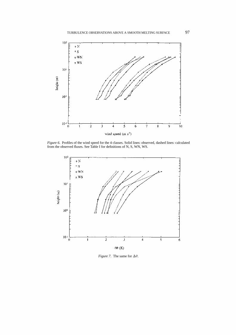
Figure 6 shows the results for the wind profiles. There is a good correspondencebetween observations and theory, except for the S category for which the observedgradient at greater height is weaker than expected. For this class, the katabatic layeris very shallow, as it contains five cases for which the wind was weaker at 30 mthan at 16 m (N contains one such case, WN and WS none). These cases will beconsidered below. The slightly different slopes for the other three classes are notsignificant in view of the possible error in the observed fluxes.

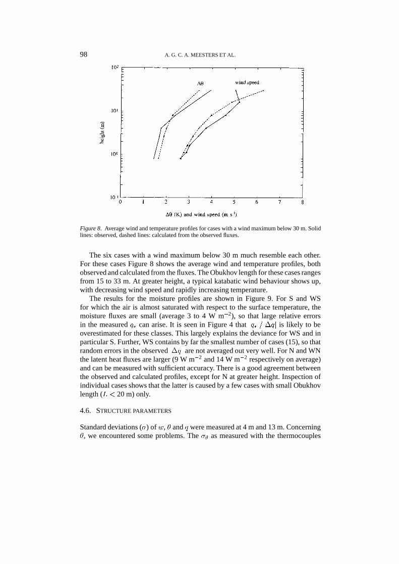
Figure 7 shows the results for the potential temperature profiles. The strongrandom variations in the observed �

�that were seen in Figure 3 cause shifts of

the calculated with respect to the observed profiles, which are largely averaged outhowever. Further, the observed temperatures have undergone large (but objective)calibration shifts that were necessary since the sensors were not aspirated. Hencethe results are not accurate enough to test the theory on radiation influence that wasdiscussed in Section 4.3. The major difference between calculated and observedprofiles occurs again at greater height for class S for which cases are includedwith a shallow boundary layer. At lower height, the observed gradient for WSseems larger than the calculated gradient, and this may be caused by the fact thatthe calculated gradient is based on flux measurements at 4 m and 13 m for whichradiation absorption causes �

�to be smaller than �

�close to the surface (Appendix).

Such an effect cannot be traced for the other classes, for which temperature readingsare inaccurate because of low wind speeds (N,S), or gradients are too small to bedetermined accurately (N,WN).


Figure 6. Profiles of the wind speed for the 4 classes. Solid lines: observed, dashed lines: calculatedfrom the observed fluxes. See Table I for definitions of N, S, WN, WS.

Figure 7. The same for ��.


Figure 8. Average wind and temperature profiles for cases with a wind maximum below 30 m. Solidlines: observed, dashed lines: calculated from the observed fluxes.

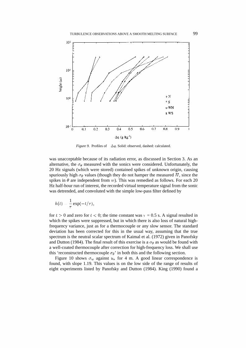
The six cases with a wind maximum below 30 m much resemble each other.For these cases Figure 8 shows the average wind and temperature profiles, bothobserved and calculated from the fluxes. The Obukhov length for these cases rangesfrom 15 to 33 m. At greater height, a typical katabatic wind behaviour shows up,with decreasing wind speed and rapidly increasing temperature.

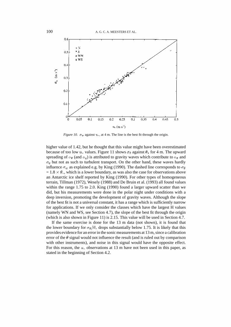
The results for the moisture profiles are shown in Figure 9. For S and WSfor which the air is almost saturated with respect to the surface temperature, themoisture fluxes are small (average 3 to 4 W m�2), so that large relative errorsin the measured q

�can arise. It is seen in Figure 4 that jq

�j=j�qj is likely to be

overestimated for these classes. This largely explains the deviance for WS and inparticular S. Further, WS contains by far the smallest number of cases (15), so thatrandom errors in the observed j�qj are not averaged out very well. For N and WNthe latent heat fluxes are larger (9 W m�2 and 14 W m�2 respectively on average)and can be measured with sufficient accuracy. There is a good agreement betweenthe observed and calculated profiles, except for N at greater height. Inspection ofindividual cases shows that the latter is caused by a few cases with small Obukhovlength (L < 20 m) only.

4.6. STRUCTURE PARAMETERS

Standard deviations (�) of w, � and q were measured at 4 m and 13 m. Concerning�, we encountered some problems. The �� as measured with the thermocouples


Figure 9. Profiles of ��q. Solid: observed, dashed: calculated.

was unacceptable because of its radiation error, as discussed in Section 3. As analternative, the �� measured with the sonics were considered. Unfortunately, the20 Hz signals (which were stored) contained spikes of unknown origin, causingspuriously high �� values (though they do not hamper the measured H , since thespikes in � are independent from w). This was remedied as follows. For each 20Hz half-hour run of interest, the recorded virtual temperature signal from the sonicwas detrended, and convoluted with the simple low-pass filter defined by

h(t) =1�

exp(�t=�);

for t > 0 and zero for t < 0; the time constant was � = 0.5 s. A signal resulted inwhich the spikes were suppressed, but in which there is also loss of natural high-frequency variance, just as for a thermocouple or any slow sensor. The standarddeviation has been corrected for this in the usual way, assuming that the truespectrum is the neutral scalar spectrum of Kaimal et al. (1972) given in Panofskyand Dutton (1984). The final result of this exercise is a �� as would be found witha well-coated thermocouple after correction for high-frequency loss. We shall usethis ‘reconstructed thermocouple ��’ in both this and the following section.

Figure 10 shows �w against u�

for 4 m. A good linear correspondence isfound, with slope 1.19. This values is on the low side of the range of results ofeight experiments listed by Panofsky and Dutton (1984). King (1990) found a


Figure 10. �w against u�, at 4 m. The line is the best fit through the origin.

higher value of 1.42, but he thought that this value might have been overestimatedbecause of too low u

�values. Figure 11 shows �� against �

�for 4 m. The upward

spreading of �� (and �q) is attributed to gravity waves which contribute to �� and�q but not as such to turbulent transport. On the other hand, these waves hardlyinfluence �w as explained e.g. by King (1990). The dashed line corresponds to ��= 1.8� �

�, which is a lower boundary, as was also the case for observations above

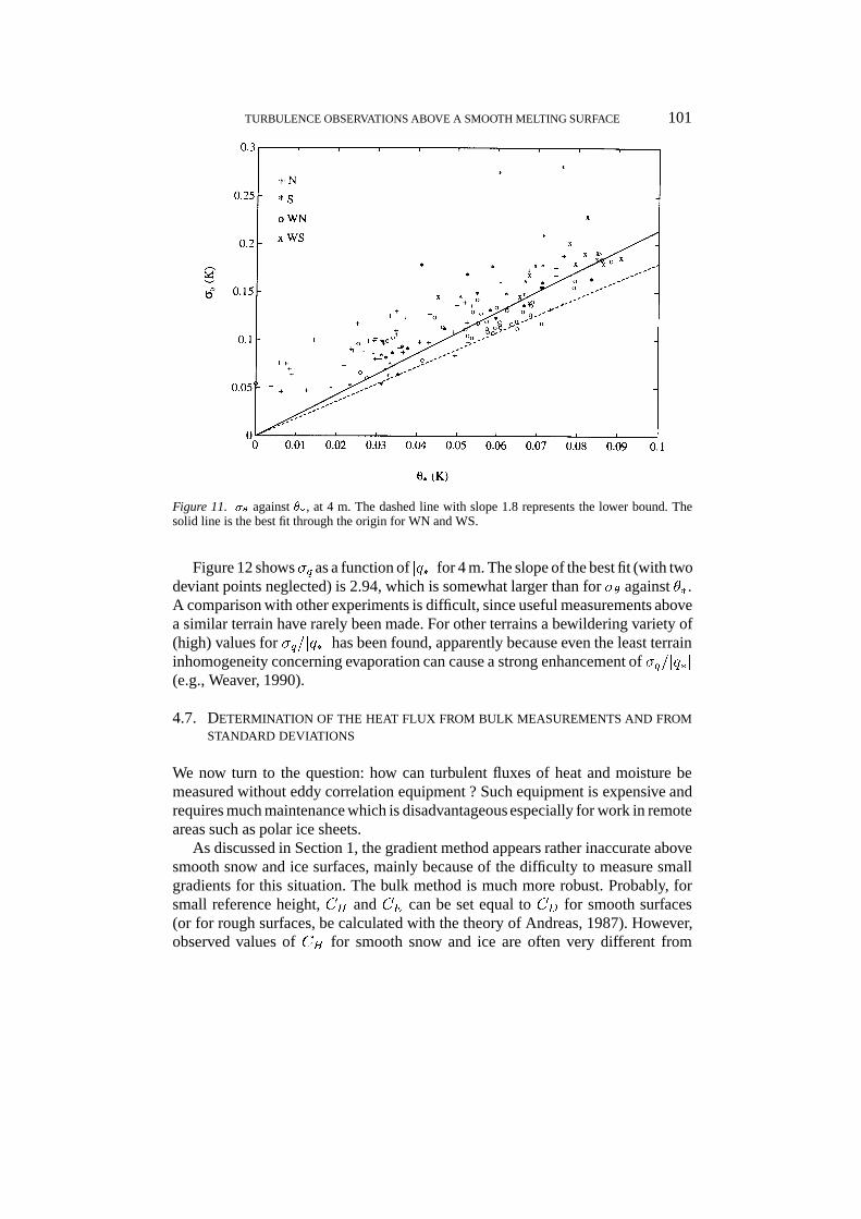
an Antarctic ice shelf reported by King (1990). For other types of homogeneousterrain, Tillman (1972), Wesely (1988) and De Bruin et al. (1993) all found valueswithin the range 1.75 to 2.0. King (1990) found a larger upward scatter than wedid, but his measurements were done in the polar night under conditions with adeep inversion, promoting the development of gravity waves. Although the slopeof the best fit is not a universal constant, it has a range which is sufficiently narrowfor applications. If we only consider the classes which have the largest H values(namely WN and WS, see Section 4.7), the slope of the best fit through the origin(which is also shown in Figure 11) is 2.15. This value will be used in Section 4.7.

If the same exercise is done for the 13 m data (not shown), it is found thatthe lower boundary for ��=�� drops substantially below 1.75. It is likely that thisprovides evidence for an error in the sonic measurements at 13 m, since a calibrationerror of the � signal would not influence the result (and is ruled out by comparisonwith other instruments), and noise in this signal would have the opposite effect.For this reason, the u

�observations at 13 m have not been used in this paper, as

stated in the beginning of Section 4.2.


Figure 11. �� against ��, at 4 m. The dashed line with slope 1.8 represents the lower bound. Thesolid line is the best fit through the origin for WN and WS.

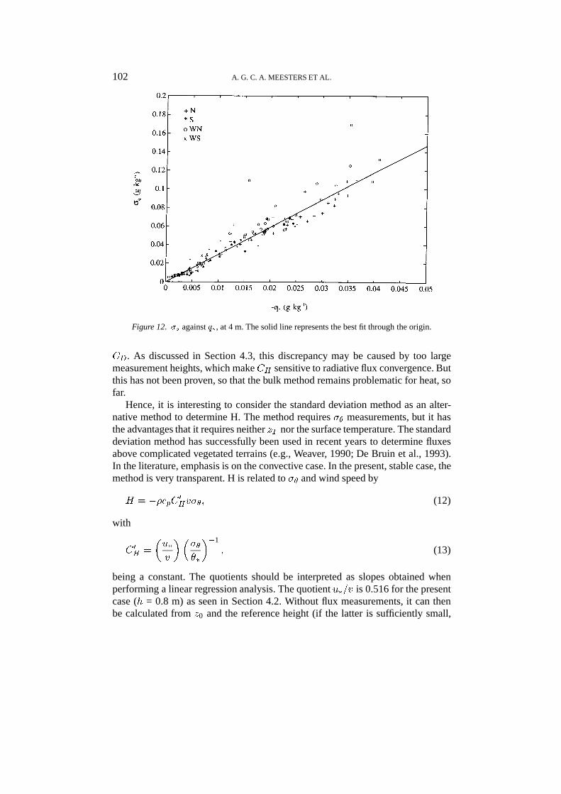
Figure 12 shows�q as a function of jq�j for 4 m. The slope of the best fit (with two

deviant points neglected) is 2.94, which is somewhat larger than for �� against ��.

A comparison with other experiments is difficult, since useful measurements abovea similar terrain have rarely been made. For other terrains a bewildering variety of(high) values for �q=jq�j has been found, apparently because even the least terraininhomogeneity concerning evaporation can cause a strong enhancement of �q=jq�j(e.g., Weaver, 1990).

4.7. DETERMINATION OF THE HEAT FLUX FROM BULK MEASUREMENTS AND FROMSTANDARD DEVIATIONS

We now turn to the question: how can turbulent fluxes of heat and moisture bemeasured without eddy correlation equipment ? Such equipment is expensive andrequires much maintenance which is disadvantageous especially for work in remoteareas such as polar ice sheets.

As discussed in Section 1, the gradient method appears rather inaccurate abovesmooth snow and ice surfaces, mainly because of the difficulty to measure smallgradients for this situation. The bulk method is much more robust. Probably, forsmall reference height, CH and CE can be set equal to CD for smooth surfaces(or for rough surfaces, be calculated with the theory of Andreas, 1987). However,observed values of CH for smooth snow and ice are often very different from


Figure 12. �q against q�, at 4 m. The solid line represents the best fit through the origin.

CD. As discussed in Section 4.3, this discrepancy may be caused by too largemeasurement heights, which make CH sensitive to radiative flux convergence. Butthis has not been proven, so that the bulk method remains problematic for heat, sofar.

Hence, it is interesting to consider the standard deviation method as an alter-native method to determine H. The method requires �� measurements, but it hasthe advantages that it requires neither zT nor the surface temperature. The standarddeviation method has successfully been used in recent years to determine fluxesabove complicated vegetated terrains (e.g., Weaver, 1990; De Bruin et al., 1993).In the literature, emphasis is on the convective case. In the present, stable case, themethod is very transparent. H is related to �� and wind speed by

H = ��cpC0

Hv��; (12)

with

C 0

H=

�u�

v

��

��1

; (13)

being a constant. The quotients should be interpreted as slopes obtained whenperforming a linear regression analysis. The quotient u

�=v is 0.516 for the present

case (h = 0.8 m) as seen in Section 4.2. Without flux measurements, it can thenbe calculated from z0 and the reference height (if the latter is sufficiently small,


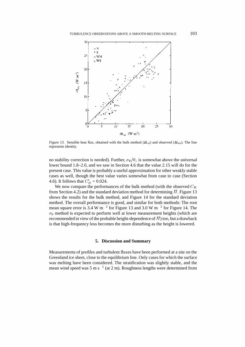
Figure 13. Sensible heat flux, obtained with the bulk method (Hcal) and observed (Hobs). The linerepresents identity.

no stability correction is needed). Further, ��=�� is somewhat above the universallower bound 1.8–2.0, and we saw in Section 4.6 that the value 2.15 will do for thepresent case. This value is probably a useful approximation for other weakly stablecases as well, though the best value varies somewhat from case to case (Section4.6). It follows that C 0

H= 0.024.

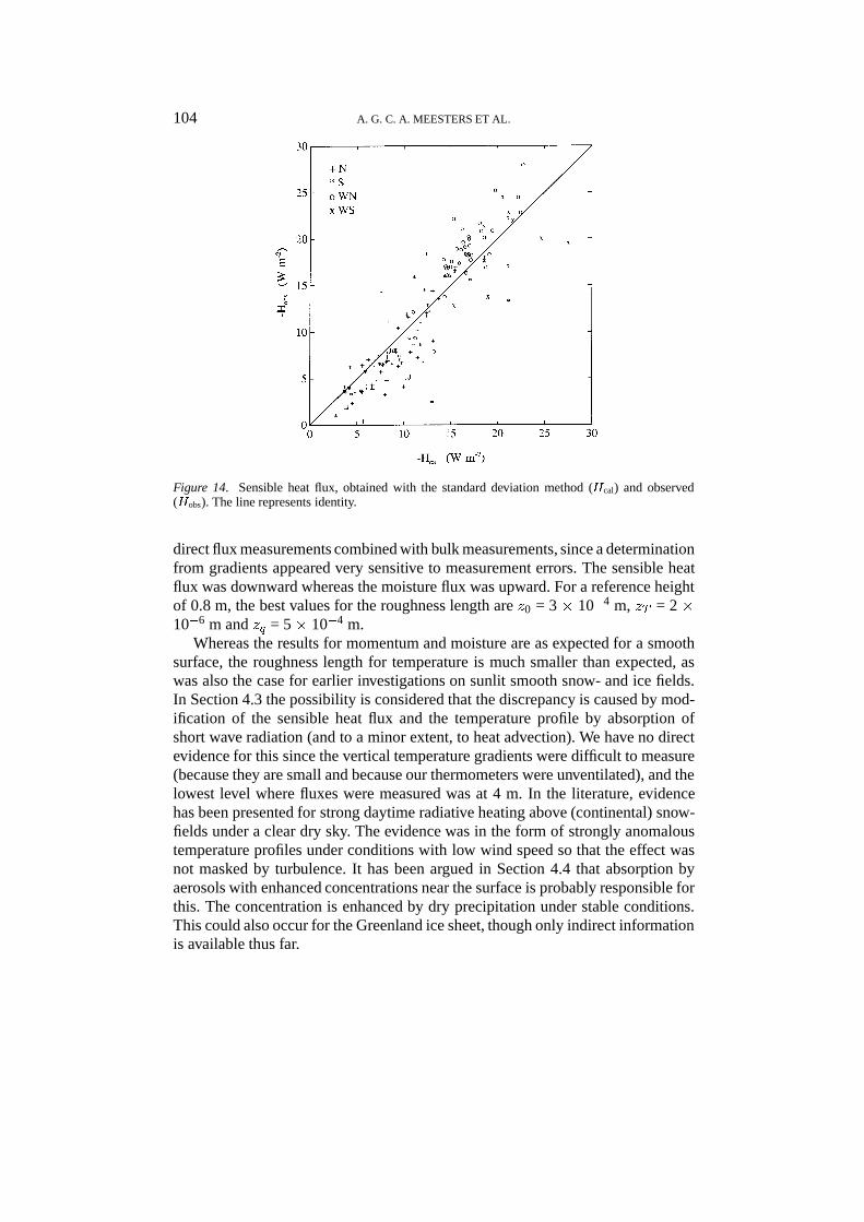
We now compare the performances of the bulk method (with the observed CHfrom Section 4.2) and the standard deviation method for determiningH . Figure 13shows the results for the bulk method, and Figure 14 for the standard deviationmethod. The overall performance is good, and similar for both methods: The rootmean square error is 3.4 W m�2 for Figure 13 and 3.0 W m�2 for Figure 14. The�� method is expected to perform well at lower measurement heights (which arerecommended in view of the probable height-dependenceofH) too, but a drawbackis that high-frequency loss becomes the more disturbing as the height is lowered.

5. Discussion and Summary

Measurements of profiles and turbulent fluxes have been performed at a site on theGreenland ice sheet, close to the equilibrium line. Only cases for which the surfacewas melting have been considered. The stratification was slightly stable, and themean wind speed was 5 m s�1 (at 2 m). Roughness lengths were determined from


Figure 14. Sensible heat flux, obtained with the standard deviation method (Hcal) and observed(Hobs). The line represents identity.

direct flux measurements combined with bulk measurements, since a determinationfrom gradients appeared very sensitive to measurement errors. The sensible heatflux was downward whereas the moisture flux was upward. For a reference heightof 0.8 m, the best values for the roughness length are z0 = 3 � 10�4 m, zT = 2 �10�6 m and zq = 5 � 10�4 m.

Whereas the results for momentum and moisture are as expected for a smoothsurface, the roughness length for temperature is much smaller than expected, aswas also the case for earlier investigations on sunlit smooth snow- and ice fields.In Section 4.3 the possibility is considered that the discrepancy is caused by mod-ification of the sensible heat flux and the temperature profile by absorption ofshort wave radiation (and to a minor extent, to heat advection). We have no directevidence for this since the vertical temperature gradients were difficult to measure(because they are small and because our thermometers were unventilated), and thelowest level where fluxes were measured was at 4 m. In the literature, evidencehas been presented for strong daytime radiative heating above (continental) snow-fields under a clear dry sky. The evidence was in the form of strongly anomaloustemperature profiles under conditions with low wind speed so that the effect wasnot masked by turbulence. It has been argued in Section 4.4 that absorption byaerosols with enhanced concentrations near the surface is probably responsible forthis. The concentration is enhanced by dry precipitation under stable conditions.This could also occur for the Greenland ice sheet, though only indirect informationis available thus far.


Male and Granger (1981) already remarked that the strong absorption whichthey observed under calm conditions above snow would disturb the validity of theflux-profile relations. It is remarkable that this has subsequently found so littleattention, in contrast with nocturnal long-wave radiation divergence. One reasonfor this is probably that the effect can be important only under special conditions.These will now be considered.

If the hypothesis is correct, anomalous behaviour by shortwave radiation absorp-tion requires a coexistence of strong insolation (a high albedo is favourable), weaksensible heat flux, and absence of convection. Over land surfaces, such conditionsseem to occur on an appreciable scale only over melting snow and ice fields. Notethat a sunlit snow surface which remains below the melting point has often a con-vective boundary layer above it. Further, sufficient supply of absorbing aerosolis required, and this is probably missing for much of Greenland in summertime(Megaw, 1982), and surely for Antarctica (Shaw, 1982). On the other hand, forcontinental snow fields there are sufficient data (Section 4.3) to believe that some-thing is going on there. Concerning the seas, it is probable that stable surface layerswith high concentrations of absorbing particles are rare.

The consequences are as follows. It should always be considered in the inter-pretation of measurements that H is height-dependent even under quasi-stationaryconditions. As seen after Equation (6), Rn � H is constant apart from advectioneffects, and since Rn diminishes as the surface is approached, the downward heatflux rises. Further, it follows that CH and zT decrease with increasing height. Thishas implications for application of the bulk method to determine sensible heatfluxes. It is customary in glaciology to use measurements at a reference heightof 1 to 2 m. According to the hypothesis, the values for zT and CH which oneshould use are larger than those obtained by profile measurements or flux-profilemeasurements at greater height, and closer to z0 and CD (provided the surface issufficiently smooth). This seems to be corroborated by measurements as discussedin Section 4.3.

Concerning rough surfaces (or rough flows), the theory of Andreas (1987) pre-dicts that z0 only depends on the surface structure, but zT =z0 becomes smaller asu�z0=� grows (see Section 4.3). His quantitative relation is confirmed by Munro

(1989), who used measurements at a height of 1 m at most. Here too, low lev-el measurements should be recommended to diminish the influence of radiationabsorption on the results. But as noted by Munro (1989), for low level measure-ments, determining the correct surface level is a problem over hilly surfaces.

Because of the difficulties with CH , an alternative method for estimating Hfrom measurements was tried, which is based on the standard deviation of thetemperature fluctuation ��. Measurements of �� with a thermocouple are muchless involved than eddy correlation measurements. Unfortunately, our thermocouplemeasurements were spoilt by insolation, due to the darkness of the sensors. Afterreliable �� values had been reconstructed from the sonic signals, it was found that�� 2.15 �

�. Such a relation is usual under slightly stable conditions, but the


proportionality factor is somewhat variable. H is proportional to v � �� with aconstant of proportionality that only depends on ��=�� and h=z0 (provided thereference height is so low that a stability correction is not necessary). An additionaladvantage of this method is that no accurate observations of the surface temperatureare needed. The method performed well for H at 4 m, and is expected to do so forlower measurement heights (which are recommended) too.

The profile measurements for wind, temperature and moisture confirm in generalthe standard flux-profile relations in the surface layer, as far as could be gatheredin view of the limited accuracy of the measurements. However, there is someindication of perturbation of the temperature profiles by radiation. For conditionswith low wind speed and comparatively strong stability, a katabatic wind maximumwas sometimes found below 30 m.

More research is needed on radiation absorption in the surface layer. An ‘in-principle easy way’ to test its importance is a comparison of zT values by dayand at night. We could not do this ourselves because of inaccurate surface tem-perature measurements at night when the surface was freezing. Aerosol absorptionmeasurements in the surface layer over glaciers would be of great value. Severaltechniques exist for this (Gerber and Hindman, 1982).

Acknowledgements

We would like to thank the technicians of the Department of Earth Sciences,Michel Groen, Theo Hamer, Hans Bakker, Johan de Lange, and the student LucBos for their valuable contributions to the VU-GIMEX expedition. The logisticalsupport of the members of the IMAU-GIMEX project and the Met-office at SøndreStrømfjord has been an essential contribution to our project. We thank J. Forrer(ETH, Zurich) and P. Smeets (of our institute) for exchange of unpublished results,and W. Greuell, R.S.W. van de Wal, and P.G. Duynkerke (University of Utrecht)for their comments on the manuscript. Substantial financial support was obtainedfrom the Dutch National Research Programme on Global Air Pollution and ClimateChange (contract 276/91-NOP).

Appendix A. Calculation of the Influence of Radiation Absorption on theMeasured Roughness Length for Temperature zT

The purpose of this Appendix is to estimate only the order of magnitude of theradiation influence, so the assumptions will be kept as simple as possible. Theturbulent heat flux H depends on height according to Equation (7). We treat S asa given quantity, and assume for convenience that the heat source, S is constantunless indicated otherwise. The relation between H and the temperature profile isgiven by Equation (9) in which the influence of stability has been neglected, andu�

is assumed constant for convenience. This completes the list of assumptions.


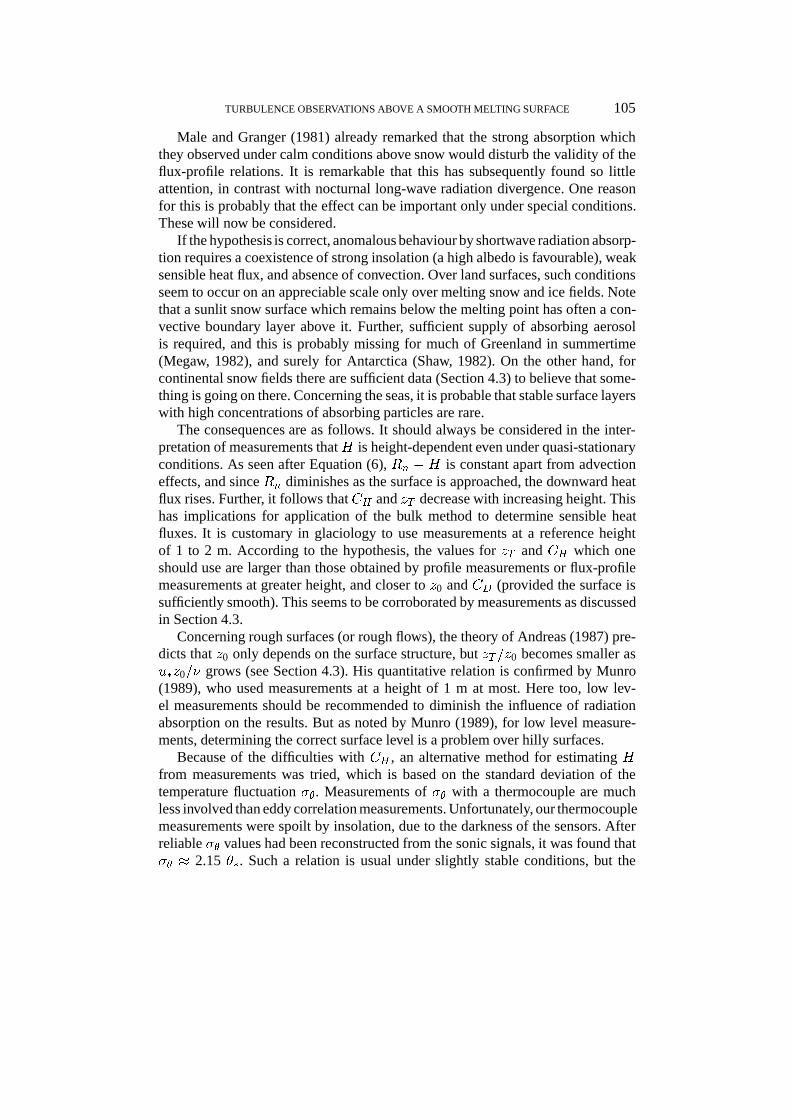
Integration of Equation (7) yields

H(z) = H(0) +Zz

0dz0S(z0): (A1)

If S is constant, the remaining integral is simply Sz. It is convenient to introducea dimensionless quantity defined by

A(z) =1

jH(0)j

Zz

0dz0S(z0);

(where we assume that H is negative). Then Equation (A1) becomes

H(z) = H(0)(1�A(z)): (A2)

Using the definition ��(z) = �H(z)=(�cpu�) yields

��(z) = �

�(0)(1�A(z)): (A3)

Combination of this with Equation (9) yields

@�

@z(z) =

��(0)k

�1�A(z)

z

�:

If S is a constant and hence A = Sz=jH(0)j, we obtain by integration that

�(z) =��(0)k

ln

z

zT;sur

!�A(z)

!: (A4)

Herein, zT;sur is the z value for which �(z), extrapolated into the viscous sublayeras usual, becomes zero (the surface is melting, or otherwise � should be interpretedas the difference of air temperature and surface temperature).

In practice, zT has to be determined from observations made at some distancefrom the surface, and owing to the fact that A 6= 0 this will yield a result that isdifferent from zT;sur. Let us first suppose that it is possible to measure � at someheight z1 and �

�at height z2. Then the observed roughness length for temperature,

zT;obs, is defined by

ln

z1

zT;obs

!= k

�(z1)

��(z2)

:

It follows from Equations (A3) and (A4) that

ln

z1

zT;obs

!=

ln

z1

zT;sur

!�A(z1)

1�A(z2): (A5)


If ��

is not measured, but �-measurements at z1 and z2 are available, zT;obs isdefined by

ln

z1

zT;obs

!=

�(z1)

�(z2)� �(z1)ln�z2

z1

�:

It follows from Equation (A4) that in this case

ln

z1

zT;obs

!=

ln

z1

zT;sur

!�A(z1)

1� [A(z2)�A(z1)]= ln(z2=z1): (A6)

Numerical examples are given in Section 4.3.

References

Ambach, W.: 1977, ‘Untersuchungen zum Energieumsatz in der Akkumulationszone desGronlandischen Inlandeises’, Meddelelser om Grønland 187–7. Bianco Lunos Bogtrykkeri A/S,Copenhagen.

Ambach, W.: 1986, ‘Nomographs for the Determination of Meltwater From Snow- and Ice Surfaces’,Berichte des Naturwissenschaftlich-Medizinischen Vereins in Innsbruck 73, 7–15.

Andreas, E. L.: 1987, ‘A Theory for the Scalar Roughness Length and the Scalar Transfer CoefficientOver Snow and Sea Ice’, Boundary-Layer Meteorol. 38, 159–184.

Bintanja, R. and Van den Broeke, M. R.: 1995, ‘Momentum and Scalar Transfer Coefficients OverAerodynamically Smooth Antarctic Surfaces’, Boundary-Layer Meteorol. 74, 89–111.

Blanchet, J. P. and Leighton, M. G.: 1981, ‘The Influence of the Refractive Index and Size Spectrumon Atmospheric Heating Due To Aerosols’, Beitr. Phys. Atmosph. 54, 143–158.

Blanchet, J. P. and List, R.: 1984, ‘On the Optical Properties of Arctic Haze’, in H. E. Gerber andA. Deepak (eds.), Aerosols and their Climatic Effects. A. Deepak Publishing, Hampton, VA, pp.179–196.

De Bruin, H. A. R., Kohsiek, W., and Van den Hurk, B. J. J. M.: 1993, ‘A Verification of Some Methodsto Determine the Fluxes of Momentum, Sensible Heat and Water Vapour using Standard Deviationand Structure Parameter of Scalar Meteorological Quantities’, Boundary-Layer Meteorol. 63,231–257.

De la Casiniere, A. C.: 1974, ‘Heat Exchange Over a Melting Snow Surface’, J. Glaciol. 13, 55–72.Duynkerke, P. G. and Van den Broeke, M. R.: 1994, ‘Surface Energy Balance and Katabatic Flow

over Glacier and Tundra during GIMEX-91’, Global Planet. Change 9, 17–28.Gallee, H., de Ghelin, O. F., and Van den Broeke, M. R.: 1995, ‘Simulation of Atmospheric Circulation

During the GIMEX 91 Experiment Using a Meso- Primitive Equations Model’, J. Climate 8,2843–2859.

Garratt, J. R. and Brost, R. A.: 1981, ‘Radiative Cooling Effect Within and Above the NocturnalBoundary Layer’, J. Atmos. Sci. 38, 2730–2746.

Gerber, H. E. and Hindman, E. E. (eds.): 1982, Light Absorption by Aerosol Particles. SpectrumPress, Hampton, VA, 420 pp.

Granger, R. J.: 1977, Energy Exchange During Melt of a Prairie Snowcover, M.Sc. Thesis, Universityof Saskatchewan, 122 pp.

Greuell, W. and Konzelmann, T.: 1994, ‘Numerical Modelling of the Energy Balance and the EnglacialTemperature of the Greenland Ice Sheet. Calculations for the ETH-Camp Location (West Green-land, 1155 m a.s.l.)’, Global Planet. Change 9, 91–114.


Hanel, G.: 1984, ‘Heating of the Atmosphere Due To Absorption of Shortwave Radiation WithinParticles’, in H. E. Gerber and A. Deepak (eds.), Aerosols and their Climatic Effects. A. DeepakPublishing, Hampton, VA, pp. 241–244.

Halberstam, I. and Schieldge, J. P.: 1981, ‘Anomalous Behaviour of the Atmospheric Surface LayerOver a Melting Snowpack’, J. Appl. Meteorol. 20, 255–265.

Henneken, E. A. C., Bink, N. J., Vugts, H. F., Cannemeijer, F., and Meesters, A. G. C. A.: 1994, ‘ACase Study of the Daily Energy Balance Near the Equilibrium Line on the Greenland Ice Sheet’,Global Planet. Change 9, 69–78.

Henneken, E. A. C., Meesters, A. G. C. A., Bink, N. J., Vugts, H. F., and Cannemeijer, F.: 1997,‘Ablation Near the Equilibrium Line on the Greenland Ice Sheet, S.W. Greenland, July 1991’, Z.Gletscherkunde Glazialgeologie 33/2, in press.

Hicks, B. B. and Martin, H. C.: 1972, ‘Atmospheric Turbulent Fluxes Over Snow’, Boundary-LayerMeteorol. 2, 496–502.

Hogstrom, U.: 1988, ‘Non-Dimensional Wind and Temperature Profiles in the Atmospheric SurfaceLayer: A Re-Evaluation’, Boundary-Layer Meteorol. 42, 55–78.

Holmgren, B.: 1971, Climate and Energy Exchange on a Subpolar Ice Cap in Summer (6 Parts).Meteorologiska Institutionen Uppsala Universitet Meddelande, pp. 107–112.

Jacobs, A. F. G. and McNaughton, K. G.: 1994, ‘The Excess Temperature of a Rigid Fast-ResponseThermometer and its Effects on the Measured Heat Flux’, J. Atmos. Oceanic Tech. 11, 680–686.

Kaimal, J. C., Wyngaard, J. C., Izumi, Y., and Cote, O. R.: 1972, ‘Spectral Characteristics of SurfaceLayer Turbulence’, Quart. J. Roy. Meteorol. Soc. 98, 563–589.

Kaimal, J. C. and Finnigan, J. J.: 1994, Atmospheric Boundary Layer Flows, Their Structure andMeasurement. Oxford University Press, New York, 289 pp.

King, J. C.: 1990, ‘Some Measurements of Turbulence Over an Antarctic Ice Shelf’, Quart. J. Roy.Meteorol. Soc. 116, 379–400.

King, J. C. and Anderson, P. S.: 1994, ‘Heat and Water Vapour Fluxes and Scalar Roughness LengthsOver an Antarctic Ice Shelf’, Boundary-Layer Meteorol. 69, 101–121.

Kondo, J. and Yamazawa, H.: 1986, ‘Bulk Transfer Coefficient Over a Snow Surface’, Boundary-Layer Meteorol. 34, 123–135.

Konzelmann, T., and Ohmura, A.: 1995, ‘Radiative Fluxes and their Impact on the Energy Balanceof the Greenland Ice Sheet’, J. Glaciol. 41, 490–502.

Male, D. H. and Granger, R. J.: 1981, ‘Snow Surface Energy Exchange’, Water Resour. Res. 17,609–627.

Meesters, A. G. C. A.: 1994, ‘Dependence of the Energy Balance of the Greenland Ice Sheet onClimate Change: Influence of Katabatic Wind and Tundra’, Quart. J. Roy. Meteorol. Soc. 120,491–517.

Meesters, A. G. C. A., Henneken, E. A. C., Bink, N. J., Vugts, H. F., and Cannemeijer, F.: 1994,‘Simulation of the Atmospheric Circulation Near the Greenland Ice Sheet Margin’, Global Planet.Change 9, 53–67.

Meesters, A. G. C. A., Bink, N. J., Henneken, E. A. C., Vugts, H. F., and Cannemeijer, F.: 1997,‘Katabatic Wind Profiles Over the Greenland Ice Sheet: Observations and Modeling’, Boundary-Layer Meteorol.

Megaw, W. J.: 1982, ‘Summer Tropospheric Aerosols Over Greenland’, in A. Deepak (ed.),Atmospheric Aerosols: Their Formation, Optical Properties, and Effects, Spectrum Press, Hamp-ton, VA, pp. 39–48.

Middleton, W. E. K.: 1958, Vision Through the Atmosphere, University of Toronto Press, 250 pp.Munro, D. S.: 1989, ‘Surface Roughness and Bulk Heat Transfer on a Glacier: Comparison With

Eddy Correlation’, J. Glaciol. 35, 343–348.Oerlemans, J. and Vugts, H. F.: 1993, ‘A Meteorological Experiment in the Melting Zone of the

Greenland Ice Sheet’, Bull. Amer. Meteorol. Soc. 74, 355–365.Oke, T. R.: 1970, ‘The Temperature Profile Near the Ground on Calm Clear Nights’, Quart. J. Roy.

Meteorol. Soc. 96, 14–23.Panofsky, H. A. and Dutton, J. A.: 1984, Atmospheric Turbulence, Wiley, New York, 397 pp.Raupach, M. R.: 1977, Atmospheric Flux Measurement by Eddy Correlation, Research Report No.

27, Flinders Institute for Atmospheric and Marine Sciences, Australia, 207 pp.


Shaw, G. E.: 1982, ‘Atmospheric Turbidity in the Polar Regions’, J. Appl. Meteorol. 21, 1080–1088.Tillman, J. E.: 1972, ‘The Indirect Determination of Stability, Heat and Momentum Fluxes in the

Atmospheric Boundary Layer From Simple Scalar Variables During Dry Unstable Conditions’,J. Appl. Meteorol. 11, 783–792.

Van de Wal, R. S. W., Bintanja, R., Boot, W., Van den Broeke, M. R., Conrads, L. A., Duynkerke, P.G., Fortuin, P., Henneken, E. A. C., Knap, W. H., Portanger, M., Vugts, H. F., and Oerlemans, J.:1995, ‘Mass Balance Measurements in the Søndre Strømfjord Area in the Period 1990–1994’, Z.Gletscherkunde Glazialgeologie 31, 57–63.

Van den Broeke, M. R.: 1996, The Atmospheric Boundary Layer Over Ice Sheets and Glaciers, Ph.D.Thesis, Utrecht University, 178 pp.

Van den Broeke, M. R., Duynkerke, P. G., and Oerlemans, J.: 1994, ‘The Observed Katabatic Flowat the Edge of the Greenland Ice Sheet during GIMEX-91’, Global Planet. Change 9, 3–15.

Van den Broeke, M. R. and Gallee, H.: 1996, ‘Observation and Simulation of Barrier Winds at theWestern Margin of the Greenland Ice Sheet’, Quart. J. Roy. Meteorol. Soc. 122, 1365–1383.

Weaver, H. L.: 1990, ‘Temperature and Humidity-Flux Variance Relations Determined by One-Dimensional Eddy Correlation’, Boundary-Layer Meteorol. 53, 77–91.

Welch, R. and Zdunkowski, W.: 1976, ‘A Radiation Model of the Polluted Atmospheric BoundaryLayer’, J. Atmos. Sci. 33, 2170–2184.

Wesely, M. L.: 1988, ‘Use of Variance Techniques to Measure Dry Air-Surface Exchange Rates’,Boundary-Layer Meteorol. 44, 13–31.

Documents

Turbulence Observations Above a Smooth Melting Surface on the Greenland Ice Sheet