Computers & Geosciences 61 (2013) 1–10

Contents lists available at ScienceDirect

Computers & Geosciences

0098-30http://d

n Tel.:E-m

journal homepage: www.elsevier.com/locate/cageo

TURBO2: A MATLAB simulation to study the effects of bioturbationon paleoceanographic time series

Martin H. Trauth n

Institut für Erd- und Umweltwissenschaften, Universität Potsdam, 14476 Potsdam, Germany

a r t i c l e i n f o

Article history:Received 1 February 2013Received in revised form4 May 2013Accepted 16 May 2013Available online 23 May 2013

Keywords:BioturbationModelingMATLABDeep-sea recordsForaminiferaStable oxygen isotopes

04/$ - see front matter & 2013 Elsevier Ltd. Ax.doi.org/10.1016/j.cageo.2013.05.003

+49 331 977 5810; fax: +49 331 977 5700.ail addresses: trauth@geo.uni-potsdam.de, tra

a b s t r a c t

Bioturbation (or benthic mixing) causes significant distortions in marine stable isotope signals and otherpalaeoceanographic records. Although the influence of bioturbation on these records is well known it hasrarely been dealt systematically. The MATLAB program called TURBO2 can be used to simulate the effectof bioturbation on individual sediment particles. It can therefore be used to model the distortion of allphysical, chemical, and biological signals in deep-sea sediments, such as Mg/Ca ratios and UK37-basedsea-surface temperature (SST) variations. In particular, it can be used to study the distortions inpaleoceanographic records that are based on individual sediment particles, such as SST records basedon foraminifera assemblages. Furthermore, TURBO2 provides a tool to study the effect of benthic mixingof isotope signals such as 14C, δ18O, and δ13C, measured in a stratigraphic carrier such as foraminiferashells.

& 2013 Elsevier Ltd. All rights reserved.

1. Introduction

Bioturbation (or benthic mixing) causes significant dis-tortions in the stable isotope records preserved in deep-seasediments (Fig. 1) (Berger and Heath, 1968; Peng et al., 1977,1979; Schiffelbein, 1984, 1985; Trauth, 1998a; Anderson, 2001;Leuschner et al., 2002; Charbit et al., 2002; Lowemark and Grootes,2004; Lowemark et al., 2008; Hughes et al., 2009). The process ofbioturbation has previously been quantified, in particular withregard to the thickness of the mixed layer in deep-sea sedimentsand the overall mixing intensity in the uppermost layers of thesedimentary column (e.g. Peng et al., 1979; Erlenkeuser, 1980;Berger and Killingley, 1982; Thomson et al., 1993, 1995, 2000;Trauth et al., 1997; Henderson et al., 1999; Smith and Rabouille,2002; Teal et al., 2010; Heard et al., 2008). Attempts have also beenmade to deconvolve the effects of bioturbation, for instance byremoving the resulting noise in isotope records (e.g. Trauth,1998b), or the effects of amplitude reduction and phase shifts(Ruddiman et al., 1976; Berger et al., 1977; Bard et al., 1987),sometimes even being able to take into account variations inmixing intensity through time (Trauth, 1995). The process ofbenthic mixing has also been modeled in many ways to predictits influence on different time scales, as a diffusion process (Bergerand Heath, 1968; Shull, 2001), a frequency-domain process

ll rights reserved.

uth@uni-potsdam.de

(Schiffelbein, 1985), a Markov-chain type single particle process(Foster, 1985; Trauth, 1998a), or a mixed diffusion-single particleprocess (Boudreau et al., 2001; Choi et al., 2002). Some authorshave identified the particular importance of time-dependentvariations in mixing intensity in their models (Trauth, 1998a;Charbit et al., 2002). Others have focused on the size dependencyof the bioturbation process, for instance to explain age differencesbetween different sized foraminifera shells (Erlenkeuser, 1980;Shull and Yasuda, 2001; Bard, 2007).

The TURBO bioturbation algorithm published in 1998 (Trauth,1998a) can be used to simulate the effects of benthic mixing onindividual sediment particles such as foraminifera tests. Theadvantage of this model is that it allows users of the program tostudy the effect of bioturbation on isotopic signals such as 14C,δ18O, and δ13C from stratigraphic carriers such as foraminifera. It isalso able to simulate the effect that a small sample size (i.e. a smallnumber of foraminifera tests with isotopic measurements) has onthe noise level of an isotope record. Most studies have onlymeasured 5 benthic or 20–40 planktonic foraminifera tests toobtain a stable isotope record (e.g. Boyle, 1984; Schiffelbein andHills, 1984; Trauth, 1998b). Replicate or duplicate measurements,made to determine the accuracy of the isotope measurementsfrom deep-sea cores, are rare (Killingley et al., 1981; Schiffelbeinand Hills, 1984; Trauth, 1995, 1998b). The disadvantage of TURBO,however, is that it was written in FORTRAN77. This programminglanguage is very inefficient in daily use compared to increasinglypopular numerical computer programming languages such as theopen-source freeware Python (http://python.org), or commercial

0 50 100 150 200

0.5

1

1.5

2

2.5

3

3.5

4

4.5

Core Depth (cm)

δ18 O

(‰ v

s. P

DB

)δ1

8 O (‰

vs.

PD

B)

0 50 100 150 200

0.5

1

1.5

2

2.5

3

3.5

Core Depth (cm)

G. bulloidesN. pachyderma (s)

1st measurement G. bulloides2nd measurement G. bulloides

Holocene

Termination

Glacial

Ib

Ib?

Ia

Ia

17049-6

Holocene

TerminationGlacial

Ib?

Ia

17049-6

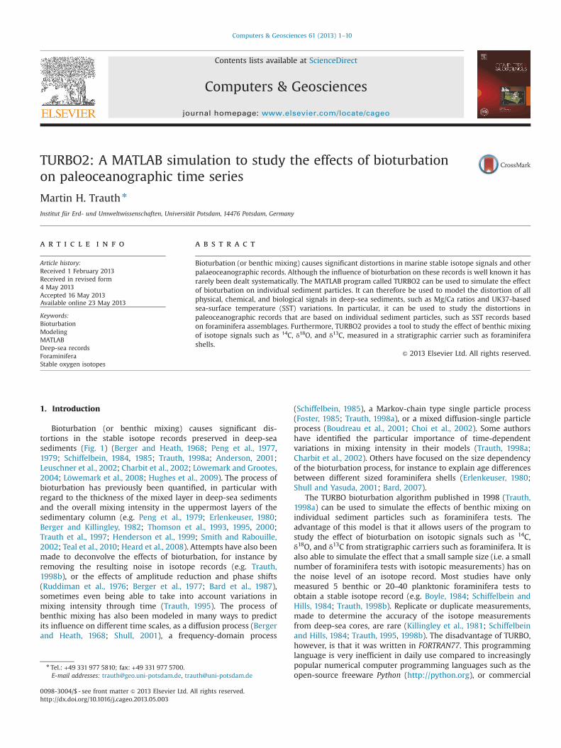
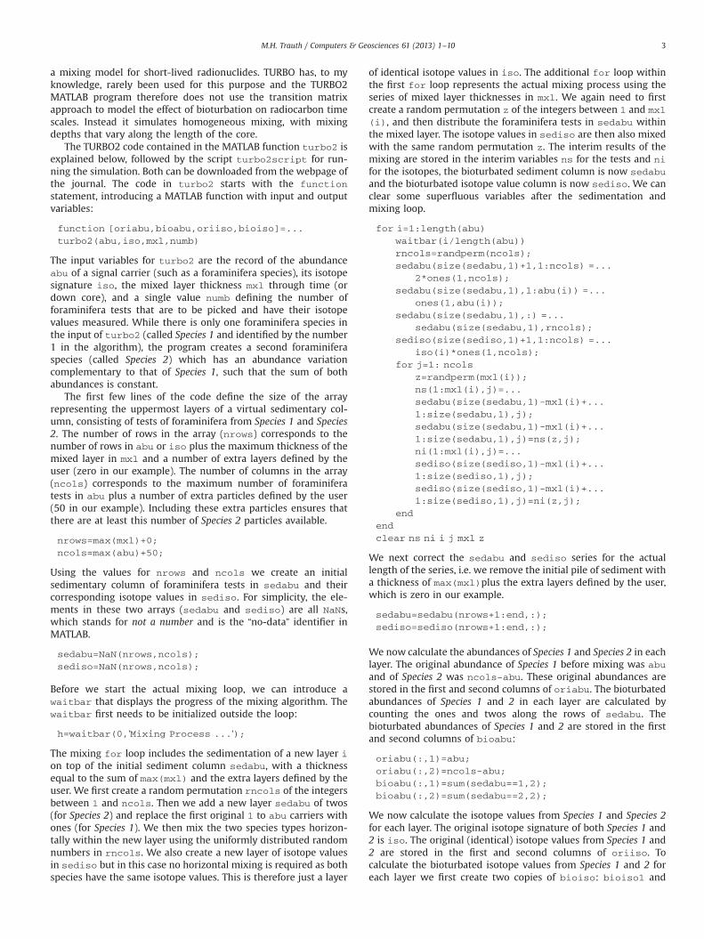
Fig. 1. (A) Real δ18O oxygen isotope record for planktonic foraminifera species G.bulloides (blue circles) and N. pachyderma (sinistral) (red squares) in deep-sea core17049-6 (Rockall Plateau, east Atlantic, 55.26N 26.73W, 3331 m water depth).(B) Duplicate record of oxygen isotope measurements on G. bulloides from the samecore. Stable isotope analyses were performed on multi-shell samples of 20 testseach. Sedimentation rates were around 10 cm kyr−1 during the Holocene andaround 6 cm kyr−1 during the glacial period (Jung, 1996). Sampling interval is2.5 cm, corresponding to 250 yr during the Holocene and 240 yr during the glacialperiod. The thickness of the homogeneous mixed layer is around 11 cm for theHolocene and around 14 cm for the glacial period, using the equation by Trauthet al. (1997) to reconstruct the mixing depth on the basis of organic carbon flux atthe seafloor. (For interpretation of the references to color in this figure legend, thereader is referred to the web version of this article.)

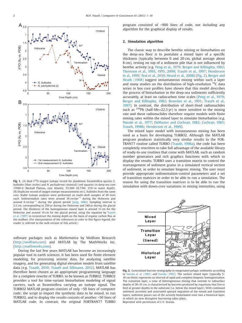
Fig. 2. Generalized burrow stratigraphy in oxygenated pelagic sediments accordingto Savrda et al. (1991) and Savrda (1992). The surface mixed layer (typically 5–10 cm thick) represents an interval of rapid and complete biogenic homogenization.The transition layer, a zone of heterogeneous mixing that extends to subsurfacedepths of 20–35 cm, is characterized by burrows produced by organisms that live orfeed at greater depths in the substrate (i.e. below the mixed layer). With continuedsediment accretion and associated upward migration of the mixed and transitionlayers, sediment passes out of the actively bioturbated zone into a historical layer,in which no new disruptive burrowing takes place.Reprinted with permission of C.V. Svarda.

M.H. Trauth / Computers & Geosciences 61 (2013) 1–102

software packages such as Mathematica by Wolfram Research(http://wolfram.com) and MATLAB by The MathWorks Inc.(http://mathworks.com).

During the last few years MATLAB has become an increasinglypopular tool in earth sciences. It has been used for finite elementmodeling, for processing seismic data, for analyzing satelliteimagery, and for generating digital elevation models from satellitedata (e.g. Trauth, 2010; Trauth and Sillmann, 2012). MATLAB hastherefore been chosen as an appropriate programming languagefor a complete rewrite of TURBO, to be known as TURBO2. TURBO2provides a tool for time-variant bioturbation modeling of signalcarriers, such as foraminifera carrying an isotope signal. TheTURBO2 MATLAB program consists of only ∼50 lines of computercode; the script to import the synthetic data to be mixed, to runTURBO2, and to display the results consists of another ∼50 lines ofMATLAB code. In contrast, the original FORTRAN77 TURBO

program consisted of ∼900 lines of code, not including anyalgorithm for the graphical display of results.

2. Simulation algorithm

The classic way to describe benthic mixing or bioturbation onthe deep-sea floor is to postulate a mixed layer of a specificthickness (typically between 0 and 20 cm, global average about8 cm), resting on top of a sediment pile that is not influenced bybenthic activity (e.g. Peng et al., 1979; Berger and Killingley, 1982;Thomson et al., 1993, 1995, 2000; Trauth et al., 1997; Hendersonet al., 1999; Teal et al., 2010; Heard et al., 2008) (Fig. 2). Berger andHeath (1968) suggest instantaneous mixing within such a layerand many studies on the distribution of high-resolution 14C dataseries in box core profiles have shown that this model describesthe process of bioturbation in the deep-sea sediments sufficientlyaccurately, at least on radiocarbon time scales (Peng et al., 1979;Berger and Killingley, 1982; Broecker et al., 1991; Trauth et al.,1997). In contrast, the distribution of short-lived radionuclidessuch as 210Pb (half-life=22.3 yr) is more sensitive to the mixingrate and these radionuclides therefore require models with finitemixing rates within the mixed layer to simulate bioturbation (e.g.Nozaki et al., 1977; DeMaster and Cochran, 1982; Cochran, 1985;Trauth, 1998b; Henderson et al., 1999).

The mixed layer model with instantaneous mixing has beenused as a basis for developing TURBO2. Although the MATLABprogram produces statistically very similar results to the FOR-TRAN77 routine called TURBO (Trauth, 1998a), the code has beencompletely rewritten to take full advantage of the available libraryof ready-to-use routines that come with MATLAB, such as randomnumber generators and rich graphics functions with which todisplay the results. TURBO uses a transition matrix to control therearrangement of sediment grains in a simulated vertical sectionof sediment, in order to simulate biogenic mixing. The user mustprovide appropriate sedimentation-control parameters and a setof transition matrices in order to be able to run a simulation. Thereason for using the transition matrices is to be able to run thesimulation with down-core variations in mixing intensities, using

M.H. Trauth / Computers & Geosciences 61 (2013) 1–10 3

a mixing model for short-lived radionuclides. TURBO has, to myknowledge, rarely been used for this purpose and the TURBO2MATLAB program therefore does not use the transition matrixapproach to model the effect of bioturbation on radiocarbon timescales. Instead it simulates homogeneous mixing, with mixingdepths that vary along the length of the core.

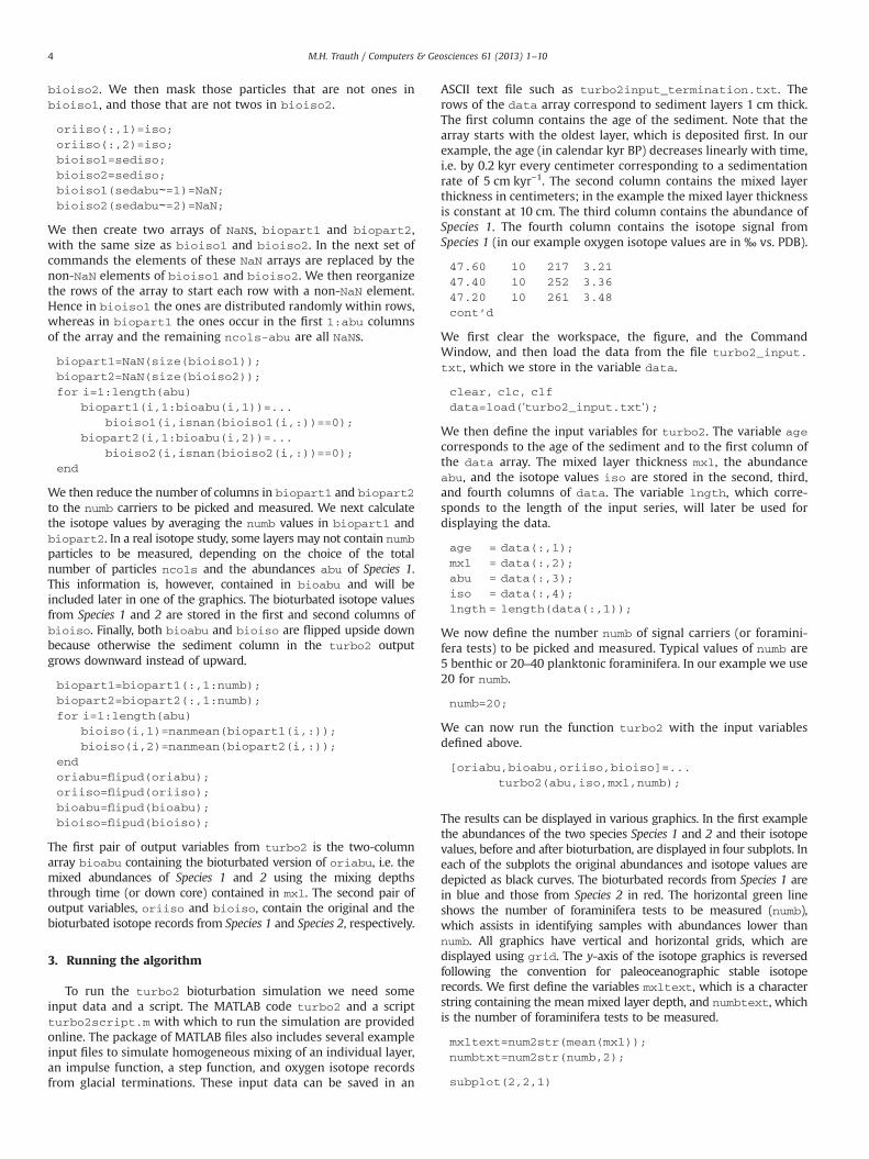
The TURBO2 code contained in the MATLAB function turbo2 isexplained below, followed by the script turbo2script for run-ning the simulation. Both can be downloaded from the webpage ofthe journal. The code in turbo2 starts with the function

statement, introducing a MATLAB function with input and outputvariables:

function [oriabu,bioabu,oriiso,bioiso]=...

turbo2(abu,iso,mxl,numb)

The input variables for turbo2 are the record of the abundanceabu of a signal carrier (such as a foraminifera species), its isotopesignature iso, the mixed layer thickness mxl through time (ordown core), and a single value numb defining the number offoraminifera tests that are to be picked and have their isotopevalues measured. While there is only one foraminifera species inthe input of turbo2 (called Species 1 and identified by the number1 in the algorithm), the program creates a second foraminiferaspecies (called Species 2) which has an abundance variationcomplementary to that of Species 1, such that the sum of bothabundances is constant.

The first few lines of the code define the size of the arrayrepresenting the uppermost layers of a virtual sedimentary col-umn, consisting of tests of foraminifera from Species 1 and Species2. The number of rows in the array (nrows) corresponds to thenumber of rows in abu or iso plus the maximum thickness of themixed layer in mxl and a number of extra layers defined by theuser (zero in our example). The number of columns in the array(ncols) corresponds to the maximum number of foraminiferatests in abu plus a number of extra particles defined by the user(50 in our example). Including these extra particles ensures thatthere are at least this number of Species 2 particles available.

nrows=max(mxl)+0;

ncols=max(abu)+50;

Using the values for nrows and ncols we create an initialsedimentary column of foraminifera tests in sedabu and theircorresponding isotope values in sediso. For simplicity, the ele-ments in these two arrays (sedabu and sediso) are all NaNs,which stands for not a number and is the “no-data” identifier inMATLAB.

sedabu=NaN(nrows,ncols);

sediso=NaN(nrows,ncols);

Before we start the actual mixing loop, we can introduce awaitbar that displays the progress of the mixing algorithm. Thewaitbar first needs to be initialized outside the loop:

h=waitbar(0,'Mixing Process ...');

The mixing for loop includes the sedimentation of a new layer ion top of the initial sediment column sedabu, with a thicknessequal to the sum of max(mxl) and the extra layers defined by theuser. We first create a random permutation rncols of the integersbetween 1 and ncols. Then we add a new layer sedabu of twos(for Species 2) and replace the first original 1 to abu carriers withones (for Species 1). We then mix the two species types horizon-tally within the new layer using the uniformly distributed randomnumbers in rncols. We also create a new layer of isotope valuesin sediso but in this case no horizontal mixing is required as bothspecies have the same isotope values. This is therefore just a layer

of identical isotope values in iso. The additional for loop withinthe first for loop represents the actual mixing process using theseries of mixed layer thicknesses in mxl. We again need to firstcreate a random permutation z of the integers between 1 and mxl

(i), and then distribute the foraminifera tests in sedabu withinthe mixed layer. The isotope values in sediso are then also mixedwith the same random permutation z. The interim results of themixing are stored in the interim variables ns for the tests and ni

for the isotopes, the bioturbated sediment column is now sedabu

and the bioturbated isotope value column is now sediso. We canclear some superfluous variables after the sedimentation andmixing loop.

for i=1:length(abu)

waitbar(i/length(abu))

rncols=randperm(ncols);

sedabu(size(sedabu,1)+1,1:ncols) =...

2*ones(1,ncols);

sedabu(size(sedabu,1),1:abu(i)) =...

ones(1,abu(i));

sedabu(size(sedabu,1),:) =...

sedabu(size(sedabu,1),rncols);

sediso(size(sediso,1)+1,1:ncols) =...

iso(i)*ones(1,ncols);

for j=1: ncols

z=randperm(mxl(i));

ns(1:mxl(i),j)=...

sedabu(size(sedabu,1)-mxl(i)+...

1:size(sedabu,1),j);

sedabu(size(sedabu,1)-mxl(i)+...

1:size(sedabu,1),j)=ns(z,j);

ni(1:mxl(i),j)=...

sediso(size(sediso,1)-mxl(i)+...

1:size(sediso,1),j);

sediso(size(sediso,1)-mxl(i)+...

1:size(sediso,1),j)=ni(z,j);

end

end

clear ns ni i j mxl z

We next correct the sedabu and sediso series for the actuallength of the series, i.e. we remove the initial pile of sediment witha thickness of max(mxl)plus the extra layers defined by the user,which is zero in our example.

sedabu=sedabu(nrows+1:end,:);

sediso=sediso(nrows+1:end,:);

We now calculate the abundances of Species 1 and Species 2 in eachlayer. The original abundance of Species 1 before mixing was abu

and of Species 2 was ncols-abu. These original abundances arestored in the first and second columns of oriabu. The bioturbatedabundances of Species 1 and 2 in each layer are calculated bycounting the ones and twos along the rows of sedabu. Thebioturbated abundances of Species 1 and 2 are stored in the firstand second columns of bioabu:

oriabu(:,1)=abu;

oriabu(:,2)=ncols-abu;

bioabu(:,1)=sum(sedabu==1,2);

bioabu(:,2)=sum(sedabu==2,2);

We now calculate the isotope values from Species 1 and Species 2for each layer. The original isotope signature of both Species 1 and2 is iso. The original (identical) isotope values from Species 1 and2 are stored in the first and second columns of oriiso. Tocalculate the bioturbated isotope values from Species 1 and 2 foreach layer we first create two copies of bioiso: bioiso1 and

M.H. Trauth / Computers & Geosciences 61 (2013) 1–104

bioiso2. We then mask those particles that are not ones inbioiso1, and those that are not twos in bioiso2.

oriiso(:,1)=iso;

oriiso(:,2)=iso;

bioiso1=sediso;

bioiso2=sediso;

bioiso1(sedabu∼=1)=NaN;bioiso2(sedabu∼=2)=NaN;

We then create two arrays of NaNs, biopart1 and biopart2,with the same size as bioiso1 and bioiso2. In the next set ofcommands the elements of these NaN arrays are replaced by thenon-NaN elements of bioiso1 and bioiso2. We then reorganizethe rows of the array to start each row with a non-NaN element.Hence in bioiso1 the ones are distributed randomly within rows,whereas in biopart1 the ones occur in the first 1:abu columnsof the array and the remaining ncols-abu are all NaNs.

biopart1=NaN(size(bioiso1));

biopart2=NaN(size(bioiso2));

for i=1:length(abu)

biopart1(i,1:bioabu(i,1))=...

bioiso1(i,isnan(bioiso1(i,:))==0);

biopart2(i,1:bioabu(i,2))=...

bioiso2(i,isnan(bioiso2(i,:))==0);

end

We then reduce the number of columns in biopart1 and biopart2

to the numb carriers to be picked and measured. We next calculatethe isotope values by averaging the numb values in biopart1 andbiopart2. In a real isotope study, some layers may not contain numb

particles to be measured, depending on the choice of the totalnumber of particles ncols and the abundances abu of Species 1.This information is, however, contained in bioabu and will beincluded later in one of the graphics. The bioturbated isotope valuesfrom Species 1 and 2 are stored in the first and second columns ofbioiso. Finally, both bioabu and bioiso are flipped upside downbecause otherwise the sediment column in the turbo2 outputgrows downward instead of upward.

biopart1=biopart1(:,1:numb);

biopart2=biopart2(:,1:numb);

for i=1:length(abu)

bioiso(i,1)=nanmean(biopart1(i,:));

bioiso(i,2)=nanmean(biopart2(i,:));

end

oriabu=flipud(oriabu);

oriiso=flipud(oriiso);

bioabu=flipud(bioabu);

bioiso=flipud(bioiso);

The first pair of output variables from turbo2 is the two-columnarray bioabu containing the bioturbated version of oriabu, i.e. themixed abundances of Species 1 and 2 using the mixing depthsthrough time (or down core) contained in mxl. The second pair ofoutput variables, oriiso and bioiso, contain the original and thebioturbated isotope records from Species 1 and Species 2, respectively.

3. Running the algorithm

To run the turbo2 bioturbation simulation we need someinput data and a script. The MATLAB code turbo2 and a scriptturbo2script.m with which to run the simulation are providedonline. The package of MATLAB files also includes several exampleinput files to simulate homogeneous mixing of an individual layer,an impulse function, a step function, and oxygen isotope recordsfrom glacial terminations. These input data can be saved in an

ASCII text file such as turbo2input_termination.txt. Therows of the data array correspond to sediment layers 1 cm thick.The first column contains the age of the sediment. Note that thearray starts with the oldest layer, which is deposited first. In ourexample, the age (in calendar kyr BP) decreases linearly with time,i.e. by 0.2 kyr every centimeter corresponding to a sedimentationrate of 5 cm kyr−1. The second column contains the mixed layerthickness in centimeters; in the example the mixed layer thicknessis constant at 10 cm. The third column contains the abundance ofSpecies 1. The fourth column contains the isotope signal fromSpecies 1 (in our example oxygen isotope values are in ‰ vs. PDB).

47.60 1

0 2 17 3 .21

47.40 1

0 2 52 3 .36

47.20 1

0 2 61 3 .48

cont’d

We first clear the workspace, the figure, and the CommandWindow, and then load the data from the file turbo2_input.

txt, which we store in the variable data.

clear, clc, clf

data=load('turbo2_input.txt');

We then define the input variables for turbo2. The variable age

corresponds to the age of the sediment and to the first column ofthe data array. The mixed layer thickness mxl, the abundanceabu, and the isotope values iso are stored in the second, third,and fourth columns of data. The variable lngth, which corre-sponds to the length of the input series, will later be used fordisplaying the data.

age = data(:,1);

mxl = data(:,2);

abu = data(:,3);

iso = data(:,4);

lngth = length(data(:,1));

We now define the number numb of signal carriers (or foramini-fera tests) to be picked and measured. Typical values of numb are5 benthic or 20–40 planktonic foraminifera. In our example we use20 for numb.

numb=20;

We can now run the function turbo2 with the input variablesdefined above.

[oriabu,bioabu,oriiso,bioiso]=...

turbo2(abu,iso,mxl,numb);

The results can be displayed in various graphics. In the first examplethe abundances of the two species Species 1 and 2 and their isotopevalues, before and after bioturbation, are displayed in four subplots. Ineach of the subplots the original abundances and isotope values aredepicted as black curves. The bioturbated records from Species 1 arein blue and those from Species 2 in red. The horizontal green lineshows the number of foraminifera tests to be measured (numb),which assists in identifying samples with abundances lower thannumb. All graphics have vertical and horizontal grids, which aredisplayed using grid. The y-axis of the isotope graphics is reversedfollowing the convention for paleoceanographic stable isotoperecords. We first define the variables mxltext, which is a characterstring containing the mean mixed layer depth, and numbtext, whichis the number of foraminifera tests to be measured.

mxltext=num2str(mean(mxl));

numbtxt=num2str(numb,2);

subplot(2,2,1)

M.H. Trauth / Computers & Geosciences 61 (2013) 1–10 5

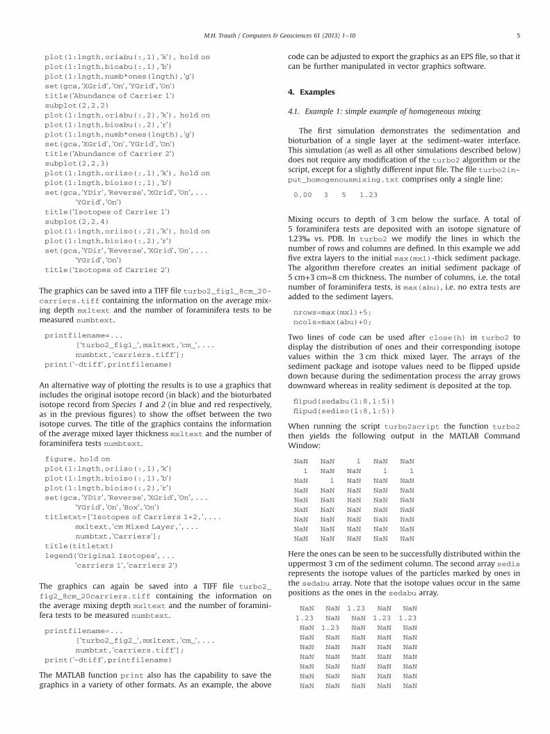
plot(1:lngth,oriabu(:,1),'k'), hold on

plot(1:lngth,bioabu(:,1),'b')plot(1:lngth,numb*ones(lngth),'g')set(gca,'XGrid','On','YGrid','On')title('Abundance of Carrier 1')subplot(2,2,2)

plot(1:lngth,oriabu(:,2),'k'), hold on

plot(1:lngth,bioabu(:,2),'r')plot(1:lngth,numb*ones(lngth),'g')set(gca,'XGrid','On','YGrid','On')title('Abundance of Carrier 2')subplot(2,2,3)

plot(1:lngth,oriiso(:,1),'k'), hold on

plot(1:lngth,bioiso(:,1),'b')set(gca,'YDir','Reverse','XGrid','On',...

'YGrid','On')title('Isotopes of Carrier 1')subplot(2,2,4)

plot(1:lngth,oriiso(:,2),'k'), hold on

plot(1:lngth,bioiso(:,2),'r')set(gca,'YDir','Reverse','XGrid','On',...

'YGrid','On')title('Isotopes of Carrier 2')

The graphics can be saved into a TIFF file turbo2_fig1_8cm_20-

carriers.tiff containing the information on the average mix-ing depth mxltext and the number of foraminifera tests to bemeasured numbtext.

printfilename=...

['turbo2_fig1_',mxltext,'cm_',...numbtxt,'carriers.tiff'];

print('-dtiff',printfilename)

An alternative way of plotting the results is to use a graphics thatincludes the original isotope record (in black) and the bioturbatedisotope record from Species 1 and 2 (in blue and red respectively,as in the previous figures) to show the offset between the twoisotope curves. The title of the graphics contains the informationof the average mixed layer thickness mxltext and the number offoraminifera tests numbtext.

figure, hold on

plot(1:lngth,oriiso(:,1),'k')plot(1:lngth,bioiso(:,1),'b')plot(1:lngth,bioiso(:,2),'r')set(gca,'YDir','Reverse','XGrid','On',...

'YGrid','On','Box','On')titletxt=['Isotopes of Carriers 1+2,',...

mxltext,'cm Mixed Layer,',...numbtxt,'Carriers'];

title(titletxt)

legend('Original Isotopes',...'carriers 1','carriers 2')

The graphics can again be saved into a TIFF file turbo2_

fig2_8cm_20carriers.tiff containing the information onthe average mixing depth mxltext and the number of foramini-fera tests to be measured numbtext.

printfilename=...

['turbo2_fig2_',mxltext,'cm_',...numbtxt,'carriers.tiff'];

print('-dtiff',printfilename)

The MATLAB function print also has the capability to save thegraphics in a variety of other formats. As an example, the above

code can be adjusted to export the graphics as an EPS file, so that itcan be further manipulated in vector graphics software.

4. Examples

4.1. Example 1: simple example of homogeneous mixing

The first simulation demonstrates the sedimentation andbioturbation of a single layer at the sediment–water interface.This simulation (as well as all other simulations described below)does not require any modification of the turbo2 algorithm or thescript, except for a slightly different input file. The file turbo2in-

put_homogenousmixing.txt comprises only a single line:

0.00

3 5 1.23

Mixing occurs to depth of 3 cm below the surface. A total of5 foraminifera tests are deposited with an isotope signature of1.23‰ vs. PDB. In turbo2 we modify the lines in which thenumber of rows and columns are defined. In this example we addfive extra layers to the initial max(mxl)-thick sediment package.The algorithm therefore creates an initial sediment package of5 cm+3 cm=8 cm thickness. The number of columns, i.e. the totalnumber of foraminifera tests, is max(abu), i.e. no extra tests areadded to the sediment layers.

nrows=max(mxl)+5;

ncols=max(abu)+0;

Two lines of code can be used after close(h) in turbo2 todisplay the distribution of ones and their corresponding isotopevalues within the 3 cm thick mixed layer. The arrays of thesediment package and isotope values need to be flipped upsidedown because during the sedimentation process the array growsdownward whereas in reality sediment is deposited at the top.

flipud(sedabu(1:8,1:5))

flipud(sediso(1:8,1:5))

When running the script turbo2script the function turbo2

then yields the following output in the MATLAB CommandWindow:

NaN

NaN 1 NaN NaN

1

NaN NaN 1 1

NaN

1 NaN NaN NaN

NaN

NaN NaN NaN NaN

NaN

NaN NaN NaN NaN

NaN

NaN NaN NaN NaN

NaN

NaN NaN NaN NaN

NaN

NaN NaN NaN NaN

NaN

NaN NaN NaN NaN

Here the ones can be seen to be successfully distributed within theuppermost 3 cm of the sediment column. The second array sedis

represents the isotope values of the particles marked by ones inthe sedabu array. Note that the isotope values occur in the samepositions as the ones in the sedabu array.

NaN

NaN 1.23 NaN NaN

1.23

NaN NaN 1.23 1.23

NaN

1.23 NaN NaN NaN

NaN

NaN NaN NaN NaN

NaN

NaN NaN NaN NaN

NaN

NaN NaN NaN NaN

NaN

NaN NaN NaN NaN

NaN

NaN NaN NaN NaN

NaN

NaN NaN NaN NaN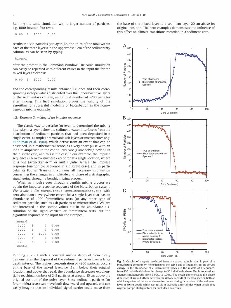

M.H. Trauth / Computers & Geosciences 61 (2013) 1–106

Running the same simulation with a larger number of particles,e.g. 1000 foraminifera tests,

0.00

3 1000 0.00

500

450

results in ∼333 particles per layer (i.e. one-third of the total withineach of the three layers) in the uppermost 3 cm of the sedimentarycolumn, as can be seen by typing

400

bioabu

350

300

f Par

ticle

s

after the prompt in the Command Window. The same simulationcan easily be repeated with different values in the input file for themixed layer thickness:

o

250True abundancebe

r

0.00

5 1000 0.00

0 20 40 60 80 100

200

150

100

50

0

500

450

400

350

300

250

200

150

100

50

0

Core Depth (cm)

0 20 40 60 80 100Core Depth (cm)

1

1.5

Bioturbated abundanceSpecies 1

True abundanceBioturbated abundanceSpecies 2

. PD

B)

Num

ber o

f Par

ticle

sN

um

and the corresponding results obtained, i.e. ones and their corre-sponding isotope values distributed over the uppermost five layersof the sedimentary column, and a total number of ∼200 particlesafter mixing. This first simulation proves the validity of thealgorithm for successful modeling of bioturbation in the homo-geneous mixing example.

4.2. Example 2: mixing of an impulse sequence

The classic way to describe (or even to determine) the mixingintensity in a layer below the sediment–water interface is from thedistribution of sediment particles that had been deposited in asingle event. Examples are volcanic ash layers or microtectites (e.g.Ruddiman et al., 1980), which derive from an event that can bedescribed, in a mathematical sense, as a very short pulse with aninfinite amplitude in the continuous case (Dirac delta function). Inthe discrete case, and this is the case in our example, the impulsesequence is zero everywhere except for at a single location, whereit is one (Kronecker delta or unit impulse series). The impulseresponse function (or sequence in a discrete case), and in parti-cular its Fourier Transform, contains all necessary informationconcerning the changes in amplitude and phase of a stratigraphicsignal going through a benthic mixing process.

When an impulse goes through a benthic mixing process weobtain the impulse response sequence of the bioturbation system.We create a file turbo2input_impulsesequence.txt withzero abundance everywhere except for a single layer that has anabundance of 1000 foraminifera tests (or any other type ofsediment particle, such as ash particles or microtectites). We arenot interested in the isotope values but in the abundance dis-tribution of the signal carriers or foraminifera tests, but thealgorithm requires some input for the isotopes.

s

2

‰ v

(cont'd)

O (

0.00 5 0 0.00

True isotope recordδ18

0.00

5 0 0.00 2.5 Bioturbated isotope 0.00 5 1000 0.00

record Species 1Bioturbated isotope

0.00 5 0 0.00

3record Species 2

0.00 5 0 0.00

0 20 40 60 80 100Core Depth (cm)

Fig. 3. Graphs of outputs produced from a turbo2 sample run. Impact of abioturbating community homogenizing the top 8 cm of sediment on an abruptchange in the abundance of a foraminifera species in the middle of a sequence,from 450 individuals below the change to 50 individuals above. The isotope valueschange simultaneously from 3.00‰ to 1.00‰. The result demonstrates the phasedifference of around 20 cm between the isotope records of the two species, both ofwhich experienced the same change in climate during deposition of the sedimentlayer at 50 cm depth, which can result in dramatic uncertainties when developingoxygen isotope stratigraphies for such deep sea cores.

(cont'd)

Running turbo2 with a constant mixing depth of 5 cm nicelydemonstrates the dispersal of the sediment particles over a largedepth interval. The highest concentration of ∼200 particles occursat the base of the mixed layer, i.e. 5 cm below their originallocation, and above that peak the abundance decreases exponen-tially reaching numbers of 2–5 particles at around 15 cm above theoriginal position of the pulse layer. Since sediment particles (orforaminifera tests) can move both downward and upward, one caneasily imagine that an individual signal carrier could move from

the base of the mixed layer to a sediment layer 20 cm above itsoriginal position. The next examples demonstrate the influence ofthis effect on climate transitions recorded in a sediment core.

1

1.5

2

2.5

3

3.5

True isotope recordBioturbated isotoperecord Species 1Bioturbated isotoperecord Species 2

Holocene

Termination

Glacial

Ib

Ia

δ18 O

(‰ v

s. P

DB

)

M.H. Trauth / Computers & Geosciences 61 (2013) 1–10 7

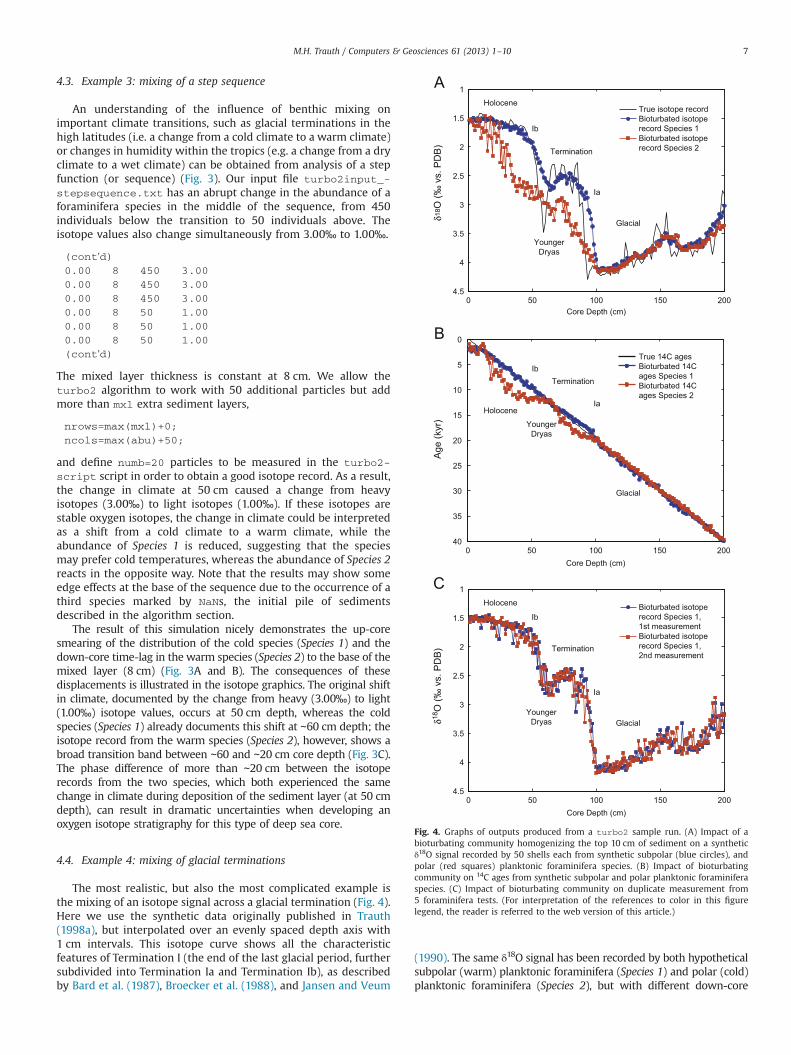
4.3. Example 3: mixing of a step sequence

An understanding of the influence of benthic mixing onimportant climate transitions, such as glacial terminations in thehigh latitudes (i.e. a change from a cold climate to a warm climate)or changes in humidity within the tropics (e.g. a change from a dryclimate to a wet climate) can be obtained from analysis of a stepfunction (or sequence) (Fig. 3). Our input file turbo2input_-

stepsequence.txt has an abrupt change in the abundance of aforaminifera species in the middle of the sequence, from 450individuals below the transition to 50 individuals above. Theisotope values also change simultaneously from 3.00‰ to 1.00‰.

Younger

4Dryas

(cont'd)

0.00 8 450 3.00

4.5

0.00 8 450 3.00

0 50 100 150 200

0.00 8 450 3.00 Core Depth (cm) 0.00 8 50 1.00

0.00

8 50 1.00 0 0.00 8 50 1.00

5

10

True 14C agesBioturbated 14Cages Species 1Bioturbated 14Cages Species 2

Holocene

TerminationIb

Ia

(cont'd)

The mixed layer thickness is constant at 8 cm. We allow theturbo2 algorithm to work with 50 additional particles but addmore than mxl extra sediment layers,

15

20

YoungerDryas

e (k

yr)

nrows=max(mxl)+0;

ncols=max(abu)+50;

0 50 100 150 200

25

30

35

40

Core Depth (cm)

Glacial

Bioturbated isotoperecord Species 1,1st measurementBioturbated isotoperecord Species 1,2nd measurement

0 50 100 150 200

1

1.5

2

2.5

3

3.5

4

4.5

Core Depth (cm)

Holocene

Termination

GlacialYounger

Dryas

Ib

Ia

δ18O

(‰ v

s. P

DB

) A

g

and define numb=20 particles to be measured in the turbo2-

script script in order to obtain a good isotope record. As a result,the change in climate at 50 cm caused a change from heavyisotopes (3.00‰) to light isotopes (1.00‰). If these isotopes arestable oxygen isotopes, the change in climate could be interpretedas a shift from a cold climate to a warm climate, while theabundance of Species 1 is reduced, suggesting that the speciesmay prefer cold temperatures, whereas the abundance of Species 2reacts in the opposite way. Note that the results may show someedge effects at the base of the sequence due to the occurrence of athird species marked by NaNs, the initial pile of sedimentsdescribed in the algorithm section.

The result of this simulation nicely demonstrates the up-coresmearing of the distribution of the cold species (Species 1) and thedown-core time-lag in the warm species (Species 2) to the base of themixed layer (8 cm) (Fig. 3A and B). The consequences of thesedisplacements is illustrated in the isotope graphics. The original shiftin climate, documented by the change from heavy (3.00‰) to light(1.00‰) isotope values, occurs at 50 cm depth, whereas the coldspecies (Species 1) already documents this shift at ∼60 cm depth; theisotope record from the warm species (Species 2), however, shows abroad transition band between ∼60 and ∼20 cm core depth (Fig. 3C).The phase difference of more than ∼20 cm between the isotoperecords from the two species, which both experienced the samechange in climate during deposition of the sediment layer (at 50 cmdepth), can result in dramatic uncertainties when developing anoxygen isotope stratigraphy for this type of deep sea core.

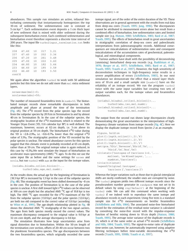
Fig. 4. Graphs of outputs produced from a turbo2 sample run. (A) Impact of abioturbating community homogenizing the top 10 cm of sediment on a syntheticδ18O signal recorded by 50 shells each from synthetic subpolar (blue circles), andpolar (red squares) planktonic foraminifera species. (B) Impact of bioturbatingcommunity on 14C ages from synthetic subpolar and polar planktonic foraminiferaspecies. (C) Impact of bioturbating community on duplicate measurement from5 foraminifera tests. (For interpretation of the references to color in this figurelegend, the reader is referred to the web version of this article.)

4.4. Example 4: mixing of glacial terminations

The most realistic, but also the most complicated example isthe mixing of an isotope signal across a glacial termination (Fig. 4).Here we use the synthetic data originally published in Trauth(1998a), but interpolated over an evenly spaced depth axis with1 cm intervals. This isotope curve shows all the characteristicfeatures of Termination I (the end of the last glacial period, furthersubdivided into Termination Ia and Termination Ib), as describedby Bard et al. (1987), Broecker et al. (1988), and Jansen and Veum

(1990). The same δ18O signal has been recorded by both hypotheticalsubpolar (warm) planktonic foraminifera (Species 1) and polar (cold)planktonic foraminifera (Species 2), but with different down-core

M.H. Trauth / Computers & Geosciences 61 (2013) 1–108

abundances. This sample run simulates an active, infaunal bio-turbating community that instantaneously homogenizes the top10 cm of sediment. The sedimentation rate is constant at5 cm kyr−1. Each sedimentation event deposits a 1 cm thick layerof new sediment that is mixed with older sediment during thesubsequent bioturbation event. Each combined sedimentation andbioturbation event therefore represents a discrete time interval of200 years. The input file turbo2input_termination.txt lookslike this:

238

47.60 10 217 3.21

237

47.40 10 252 3.36

236

47.20 10 261 3.48

235

47.00 10 222 3.60

234

46.80 10 182 3.66

233

46.60 10 185 3.58

232

46.40 10 193 3.50

cont'd

We again allow the algorithm turbo2 to work with 50 additionalparticles but this time we do not add more than mxl extra sedimentlayers,

nrows=max(mxl)+0;

ncols=max(abu)+50;

The number of measured foraminifera tests is numb=50. The biotur-bated isotopic records show remarkable discrepancies in bothamplitude and phase at around the time of the termination(Fig. 4A). The δ18O record from the polar species lags the recordfrom the subpolar species by 20 Fcm in Termination Ia and by almost40 cm in Termination Ib. In the case of the subpolar species, thestratigraphic location of the δ18O maximum, which is related to theYounger Dryas Event (YD, 11.6 calendar kyr BP) is well defined. Themaximum, however, occurs at 62 cm depth, i.e. 3 cm above itsoriginal position at 59 cm depth. The bioturbated δ18O value duringthe YD is ∼2.8–2.9‰, i.e. ∼0.6–0.7‰ lower than the original δ18Ovalue of 3.5‰. The stratigraphic position of the YD recorded by thepolar species is unclear. The mixed abundance curves for this speciessuggest that this climatic event is probably recorded at 65 cm depth,rather than at 59 cm. The original isotope value is again reduced, inthis case by ∼0.3‰.We next simulate the impact of bioturbation onaccelerator mass spectrometry (AMS) 14C ages. To do this we use thesame input file as before and the same settings for nrows andncols, but run turbo2 with age as the input for the isotope values.

[oriabu,bioabu,oriiso,bioiso]=...

turbo2(abu,age,mxl,numb);

As the results show, the actual age for the beginning of Termination Ia(18.3 kyr BP) is increased by 1.3 kyr in the case of the subpolar species(Fig. 4B). This stratigraphic event has been shifted downward by ∼8 cmin the core. The position of Termination Ia in the case of the polarspecies is unclear. A first shift toward light δ18O values can be observedat 100 cm core depth but the attached AMS 14C age of 19.8 kyr is toohigh. The AMS 14C ages recorded for the δ18O maximum of the YDfrom the subpolar species (13.0 kyr) and the polar species (12.6 kyr),are both too old compared to the correct value of 11.6 kyr (accordingto Winn et al., 1991). The age–depth relationship plotted in Fig. 4Bshows the distorted AMS 14C stratigraphy of the two signal carriers.The ages from both species mostly exceed the correct values. Themaximum discrepancy compared to the original value is 9.0 kyr at32 cm core depth, and the average discrepancy is 0.6 kyr.

The simulation illustrates how large uncertainties arise fromsignal distortion due to bioturbation. Within the 50 cm length ofthe termination core section, offsets of 20–40 cm occur between twothe planktonic foraminifera species. The age discrepancies betweenthe two foraminifera species, which originally recorded the same

isotope signal, are of the order of the entire duration of the YD. Theseobservations are in general agreement with the results from real datafrom deep-sea cores (Trauth, 1995; Jung, 1996). The discrepanciescannot be attributed to measurement errors alone but result from acombined effect of bioturbation, low sedimentation rates and limitedsample size (e.g. Hutson, 1980; Schiffelbein, 1985; Bard et al., 1987;Trauth, 1995). The effects of bioturbation result in great uncertaintiesin stratigraphic correlation of deep-sea cores and paleoclimaticinterpretations from paleoceanographic records. Additional conse-quences are miscalculations of sedimentation rates and consequentmiscalculations of the accumulation rates of geochemical, paleonto-logical, and mineralogical components.

Various authors have dealt with the possibility of deconvolving(unmixing) bioturbated deep-sea records (e.g. Ruddiman et al.,1976; Berger et al., 1977; Schiffelbein, 1985; Bard et al., 1987;Trauth, 1995; Trauth et al., 1997). However, the high sensitivity ofdeconvolution techniques to high-frequency noise results in asevere amplification of errors (Schiffelbein, 1985). In our nextsimulation we demonstrate the effect that a mixed layer thick-ness of 10 cm and a small sample size (numb=5) have on thereliability of an isotope record. We run the program turbo2

twice with the same input variables but creating two sets ofoutput variables each, for the isotope values and foraminiferaabundances.

[oriabu1,bioabu1,oriiso1,bioiso1]=...

turbo2(abu,iso,mxl,numb);

[oriabu2,bioabu2,oriiso2,bioiso2]=...

turbo2(abu,iso,mxl,numb);

The output from the second run shows large discrepancies clearlydemonstrating the great uncertainties in the interpretation of high-frequency climate variations from isotope records (Fig. 4C). Here wedisplay the duplicate isotope record from Species 2 as an example.

figure, hold on

plot(1:lngth,oriiso1(:,2),'k')plot(1:lngth,bioiso1(:,2),'b')plot(1:lngth,bioiso2(:,2),'r')set(gca,'YDir','Reverse','XGrid','On',...

'YGrid','On','Box','On')titletxt=['Isotopes of Carriers 1+2, ',...

mxltext, 'cm Mixed Layer, ',...numbtxt,'Carriers'];

title(titletxt)

legend('Original Isotopes',...'carriers 1','carriers 2')

Whereas the larger variations such as those due to glacial–interglacialshifts are nicely confirmed, the smaller ones are corrupted by noise.The turbo2 program yields two different isotope records since thepseudorandom number generator in randperm was not set to itsdefault values by using rng('default') at the beginning of theturbo2 code. We can add this command when working withturbo2 if we indeed wish to reproduce the same isotope andabundance records in each experiment. Using five tests is a standardsample size for δ18O measurements on benthic foraminifera(Schiffelbein and Hills, 1984). The associated noise-free bioturbatedrecord for the estimation of the residual noise variance is calculatedby convolving the noise-free record with the impulse-responsefunction of benthic mixing down to 10 cm depth (Hutson, 1980;Trauth, 1995). The average noise variance of the duplicate records is3%, which is of the same order as actual δ18O records (Schiffelbeinand Hills, 1984; Trauth, 1995). The signal-to-noise ratio of duplicatetime-series can, however, be automatically improved using adaptivefiltering techniques before time-variable deconvolving the δ18Orecords (Trauth, 1995, 1998b; Trauth et al., 1997).

M.H. Trauth / Computers & Geosciences 61 (2013) 1–10 9

The last simulation demonstrates time-dependent mixingintensities due to changes in benthic ecology (Trauth, 1998a;Charbit et al., 2002). Such a temporal change in mixing intensitycan be simulated by varying the value of mxl in the input fileturbo2input_variablemixing.txt. In this file the mixingdepth increases gradually by 2 cm every 20 layers, starting with0 cm (no bioturbation) at the bottom of the core and reaching8 cm at the top. The number of measured foraminifera tests isnumb=50. The simulation results clearly demonstrate the increas-ing offsets between the two records from Species 1 and Species 2,as well as the upward increase in noise levels in both sets ofrecords. A time-variable mixing intensity requires a time-variabledeconvolution technique in either the time or the frequencydomain. An example of such a deconvolution technique has beenpresented in a previous publication (Trauth, 1995). A duplicateisotope record is first adaptively filtered using an adaptive noisecanceller published by Trauth (1998b). The filtered time series isthen divided into segments, each overlapping by one sample. Theoverlapping segments are then Fourier transformed and dividedby the Fourier transformed impulse response sequence of thebioturbation process. In order to avoid the typical edge effects of aFourier transform an alternative method can be used to performthe deconvolution that uses a Wavelet transform instead of aFourier transform. The impulse response sequence used to decon-volve the sample at a particular depth in the core depends on themixed layer thickness at this depth. The mixed layer thicknessMXLcan be calculated using the equation

MXL ¼ –0:36þ 2:01� FC

from Trauth et al. (1997), where FC corresponds to the organiccarbon flux to the sea floor at the time of deposition of thatparticular layer. The thickness MXL of the bioturbated zone there-fore increases by approximately 2 cm if the food supply FCincreases by 1 g C m−2 yr−1, at least within a range of FC=1–6 g C m−2 yr−1. The combination of bioturbation modeling, adap-tive filtering, and time variant deconvolution effectively removessignal distortions due to benthic mixing.

5. Conclusions

The TURBO2 MATLAB program can be used to simulate theeffects of bioturbation on paleoceanographic signals such as thosefrom stable isotopes and radiocarbon ages, measured in a strati-graphic carrier such as foraminifera. In this simulation bioturba-tion is treated as a time-varying process responding to changingecological conditions at the water–sediment interface. It thereforeallows paleoceanographers to recognize signal distortions that areintroduced by bioturbation in combination with low sedimenta-tion rates and small sample sizes of foraminifera shells used forisotope measurements. The turbo2 MATLAB code, the script torun the simulations (turbo2script), and the example filesdiscussed within this paper are all available for download fromthe server of this journal.

Appendix A. Supplementary material

Supplementary data associated with this article can be found inthe online version at http://dx.doi.org/10.1016/j.cageo.2013.05.003.

References

Anderson, D.M., 2001. Attenuation of millennial-scale events by bioturbation inmarine sediments. Paleoceanography 16, 352–357.

Bard, E., Arnold, M., Duprat, L., Moyes, L., Dublessy, L.C., 1987. Reconstruction of thelast deglaciation: deconvolved records of δ18O profiles, micropaleontologicalvariations and accelerator mass spectrometric 14C dating. Climate Dynamics 1,102–112.

Bard, E., 2007. Paleoceanographic implications of the difference in deep-seasediment mixing between large and fine particles. Paleoceanography 16,235–239.

Berger, W.H., Heath, R.G., 1968. Vertical mixing in pelagic sediments. Journal ofMarine Research 26, 134–143.

Berger, W.H., Killingley, J.S., 1982. Box cores from the equatorial Pacific: 14Csedimentation rates and benthic mixing. Marine Geology 45, 93–125.

Berger, W.H., Johnson, R.F., Killingley, J.S., 1977. Unmixing of the deep-sea recordand the deglacial meltwater spike. Nature 269, 661–663.

Boudreau, B.P., Choi, J., Meysman, F., Francois-Carcaillet, F., 2001. Diffusion in alattice-automaton model of bioturbation by small deposit feeders. Journal ofMarine Research 59, 749–768.

Boyle, E.A., 1984. Sampling statistic limitations on benthic foraminifera chemicaland isotopic data. Marine Geology 58, 213–224.

Broecker, W.S., Andree, M., Wolfli, M., Oeschger, H., Bonani, G., Kennett, J., Peteet, D.,1988. The chronology of the last deglaciation: implications to the cause of theYounger Dryas event. Paleoceanography 3, 1–19.

Broecker, W.S., Klas, M., Clark, E., 1991. The influence of CaCO3 dissolution on coretop radiocarbon ages for deep-sea sediments. Paleoceanography 6, 593–608.

Charbit, S., Rabouille, C., Siani, G., 2002. Effects of benthic transport processes onabrupt climatic changes recorded in deep-sea sediments: a time-dependentmodeling approach. Journal of Geophysical Research 107 15-1–15-19.

Choi, J., Francois-Carcaillet, F., Boudreau, B.P., 2002. Lattice-automaton bioturbationsimulator (LABS): implementation for small deposit feeders. Computers andGeosciences 28, 213–222.

Cochran, J.K., 1985. Particle mixing rates in sediments of the eastern equatorialPacific: evidence from 210Pb, 239,240Pu and 137Cs distributions at MANOP sites.Geochimica et Cosmochimica Acta 49, 1195–1210.

DeMaster, D.J., Cochran, J.K., 1982. Particle mixing rates in deep-sea sedimentsdetermined from excess 210Pb and 32Si profiles. Earth and Planetary ScienceLetters 61, 257–271.

Erlenkeuser, H., 1980. 14C age and vertical mixing of deep-sea sediments. Earth andPlanetary Science Letters 47, 319–326.

Foster, D.W., 1985. BIOTURB: a Fortran Program to simulate the effects ofbioturbation on the vertical distribution of sediment. Computers and Geos-ciences 11, 39–54.

Heard, T., Pickering, K., Robinson, S., 2008. Milankovitch forcing of bioturbationintensity in deep-marine thin-bedded siliciclastic turbidites. Earth and Plane-tary Science Letters 272, 130–138.

Henderson, G., Lindsay, F., Slowey, N., 1999. Variation in bioturbation with waterdepth on marine slopes: a study on the Little Bahamas Bank. Marine Geology160, 105–118.

Hughes, M.W., Almond, P.C., Roering, J.J., 2009. Increased sediment transport viabioturbation at the last glacial–interglacial transition. Geology 37, 919–922.

Hutson, W.H., 1980. Bioturbation of deep-sea sediments: oxygen isotopes andstratigraphic uncertainty. Geology 8, 127–130.

Jansen, E., Veum, T., 1990. Two-step deglaciation: timing and impact on NorthAtlantic deep water circulation. Nature 343, 612–616.

Jung, S.J.A., 1996. Wassermassenaustausch zwischen NE-Atlantik und Nordmeerwährend der letzten 300.000/80.000 Jahre im Abbild stabiler O- und C-Isotope.In: Berichte aus dem Sonderforschungsbereich 313 der Universität Kiel, vol. 61,pp. 1–104.

Killingley, J.S., Johnson, R.F., Berger, W.H., 1981. Oxygen and carbon isotopes ofindividual shells of planktonic foraminifera from Ontong-Java Plateau, equator-ial Pacific. Palaeogeography, Palaeoclimatology, Palaeoecology 33, 193–204.

Leuschner, D.C., Sirocko, F., Grootes, P.M., Erlenkeuser, H., 2002. Possible influenceof Zoophycos bioturbation on radiocarbon dating and environmental inter-pretation. Marine Micropaleontology 46, 111–126.

Lowemark, L., 2004. Large age differences between planktic foraminifers caused byabundance variations and Zoophycosbioturbation. Paleoceanography 19,PA2001.

Lowemark, L., Konstantinou, K., Steinke, S., 2008. Bias in foraminiferal multispeciesreconstructions of paleohydrographic conditions caused by foraminiferalabundance variations and bioturbational mixing: a model approach. MarineGeology 256, 101–106.

Nozaki, Y., Cochran, J.K., Turekian, K.K., Keller, G., 1977. Radiocarbon and 210Pbdistribution in submersible taken deep sea cores from Project FAMOUS. Earthand Planetary Science Letters 34, 167–173.

Peng, T.H., Broecker, W.S., Kipphut, G., Shackleton, N., 1977. Benthic mixing in deepsea cores as determined by 14C dating and its implications regarding climatestratigraphy and the fate of fossil fuel CO2. In: Andersen, N.R., Malahoff, A.(Eds.), The Fate of Fossil Fuel in the Oceans. Plenum Press, New York,pp. 355–373.

Peng, T.H., Broecker, W.S., Berger, W.H., 1979. Rates of benthic mixing in deep-seasediments as determined by radioactive tracers. Quaternary Research 11,141–149.

Ruddiman, W.F., Dicus, R.L., Glover, L.K., 1976. Elimination of biotubation effects indeep-sea sediment core by deconvolution processing. In: Proceedings of theGeological Society of America Annual 1976 Meeting Abstracts, p. 1079.

Ruddiman, W.F., Jones, G.A., Peng, T.H., Glover, L.K., Glass, B.P., Liebertz, P.S., 1980.Tests of size and shape dependency in deep-sea mixing. Sedimentary Geology25, 257–276.

M.H. Trauth / Computers & Geosciences 61 (2013) 1–1010

Schiffelbein, P., 1984. Effect of benthic mixing on the information content of deep-sea stratigraphical signals. Nature 311, 651–653.

Schiffelbein, P., Hills, S., 1984. Direct assessment of stable isotope variability inplanktonic foraminifera populations. Palaeogeography, Palaeoclimatology,Palaeoecology 48, 197–213.

Schiffelbein, P., 1985. Extracting the benthic impulse response function: a con-strained deconvolution technique. Marine Geology 64, 313–336.

Shull, D.H., 2001. Transition-matrix model of bioturbation and radionuclidediagenesis. Limnology and Oceanography 46, 905–916.

Shull, D.H., Yasuda, M., 2001. Size-selective downward particle transport byCirratulid polychaetes. Journal of Marine Research 59, 453–473.

Smith, C.R., Rabouille, C., 2002. What controls the mixed-layer depth in deep-seasediments? The importance of POC flux. Limnology and Oceanography 47,418–426.

Savrda, C.E., 1992. Trace fossils and benthic oxygenation. In: Maples, C.G., West, R.R.(Eds.), Trace Fossils, Paleontological Society. University of Tennessee, Knoxville,pp. 172–196.

Savrda, C.E., Bottjer, D.J., Seilacher, A., 1991. Redox-related benthic events. In:Einsele, G., Ricken, W., Seilacher, A. (Eds.), Cycles and Events in Stratigraphy.Springer-Verlag, New York, pp. 524–571.

Teal, L., Bulling, M., Parker, E., Solan, M., 2010. Global patterns of bioturbationintensity and mixed depth of marine soft sediments. Aquatic Biology 2,207–218.

Thomson, J., Colley, S., Anderson, R., Cook, G.T., MacKenzie, A.B., Harkness, D.D.,1993. Holocene sediment fluxes in the Northeast Atlantic from 230Thexcess andradiocarbon measurements. Paleoceanography 8, 631–650.

Thomson, J., Colley, S., Anderson, R., Cook, G.T., MacKenzie, A.B., 1995. A comparisonof sediment accumulation chronologies by the radiocarbon and 230Thexcess

methods. Earth and Planetary Science Letters 133, 59–70.Thomson, J., Brown, L., Nixon, S., Cook, C.T., MacKenzie, A.B., 2000. Bioturbation and

Holocene sediment accumulation fluxes in the north-east Atlantic Ocean(Benthic Boundary Layer experiment sites). Marine Geology 169, 21–39.

Trauth, M.H., 1995. Bioturbate Signalverzerrung hochauflösender paläoozeanogra-phischer Zeitreihen. In: Berichte Reports des Geologisch-PaläontologischenInstituts der Universität Kiel, vol. 74, pp. 1–167.

Trauth, M.H., 1998a. TURBO: a dynamic-probabilistic simulation to study the effectsof bioturbation on paleoceanographic time series. Computers and Geosciences24, 433–441.

Trauth, M.H., 1998b. Noise removal from duplicate paleoceanographic time-series:the use of adaptive filtering techniques. Mathematical Geology 30, 557–574.

Trauth, M.H., Sarnthein, M., Arnold, M., 1997. Bioturbational mixing depth andcarbon flux at the seafloor. Paleoceanography 12, 517–526.

Trauth, M.H., 2010. MATLAB Recipes for Earth Sciences, Third edition, Springer,Heidelberg.

Trauth, M.H., Sillmann, E., 2012. MATLAB and Design Recipes for Earth Sciences:How to Collect, Process and Present Geoscientific Information. Springer,Heidelberg.

Winn, K., Sarnthein, M., Erlenkeuser, H., 1991. δ18O Stratigraphy and Chronology ofKiel Sediment Cores from the East Atlantic. In: Berichte-Reports Geologisch-Paläontologisches Institut der Universität Kiel, vol. 45, pp. 1–99.