Tuning-free Plug-and-Play Proximal Algorithm for Inverse ... · Tuning-free Plug-and-Play Proximal Algorithm for Inverse Imaging Problems denoiser) and the penalty parameter used

Tuning-free Plug-and-Play Proximal Algorithm for Inverse Imaging Problems

Kaixuan Wei 1 Angelica Aviles-Rivero 2 Jingwei Liang 3 Ying Fu 1 Carola-Bibiane Schnlieb 3 Hua Huang 1

Abstract

Plug-and-play (PnP) is a non-convex frameworkthat combines ADMM or other proximal algo-rithms with advanced denoiser priors. Recently,PnP has achieved great empirical success, espe-cially with the integration of deep learning-baseddenoisers. However, a key problem of PnP basedapproaches is that they require manual parametertweaking. It is necessary to obtain high-qualityresults across the high discrepancy in terms ofimaging conditions and varying scene content. Inthis work, we present a tuning-free PnP proximalalgorithm, which can automatically determine theinternal parameters including the penalty parame-ter, the denoising strength and the terminal time.A key part of our approach is to develop a pol-icy network for automatic search of parameters,which can be effectively learned via mixed model-free and model-based deep reinforcement learn-ing. We demonstrate, through numerical and vi-sual experiments, that the learned policy can cus-tomize different parameters for different states,and often more efficient and effective than exist-ing handcrafted criteria. Moreover, we discussthe practical considerations of the plugged denois-ers, which together with our learned policy yieldstate-of-the-art results. This is prevalent on bothlinear and nonlinear exemplary inverse imagingproblems, and in particular, we show promisingresults on Compressed Sensing MRI and phaseretrieval.

1. IntroductionThe problem of recovering an underlying unknown im-age x ∈ RN from noisy and/or incomplete measured datay ∈ RM is fundamental in computational imaging, in ap-plications including magnetic resonance imaging (MRI)

1School of Computer Science and Technology, Beijing Instituteof Technology, Beijing, China 2DPMMS, University of Cambridge,Cambridge, United Kingdom 3DAMTP, University of Cambridge,Cambridge, United Kingdom.

(Fessler, 2010), computed tomography (CT) (Elbakri &Fessler, 2002), microscopy (Aguet et al., 2008; Zheng et al.,2013), and inverse scattering (Katz et al., 2014; Metzleret al., 2017b). This image recovery task is often formulatedas an optimization problem that minimizes a cost function,i.e.,

minimizex∈RN

D (x) + λR (x) , (1)

where D is a data-fidelity term that ensures consistencybetween the reconstructed image and measured data. Ris a regularizer that imposes certain prior knowledge, e.g.smoothness (Osher et al., 2005; Ma et al., 2008), sparsity(Yang et al., 2010; Liao & Sapiro, 2008; Ravishankar &Bresler, 2010), low rank (Semerci et al., 2014; Gu et al.,2017) and nonlocal self-similarity (Mairal et al., 2009; Quet al., 2014), regarding the unknown image. The problem inEq. (1) is often solved by first-order iterative proximal algo-rithms, e.g. fast iterative shrinkage/thresholding algorithm(FISTA) (Beck & Teboulle, 2009) and alternating direc-tion method of multipliers (ADMM) (Boyd et al., 2011), totackle the nonsmoothness of the regularizers.

To handle the nonsmoothness caused by regularizers, first-order algorithms rely on the proximal operators (Beck &Teboulle, 2009; Boyd et al., 2011; Chambolle & Pock, 2011;Parikh et al., 2014; Geman, 1995; Esser et al., 2010) definedby

Proxσ2R(v) = argminx

(R(x) + 1

2σ2‖x− v‖22

). (2)

Interestingly, given the mathematical equivalence of theproximal operator to the regularized denoising, the proximaloperators Proxσ2R can be replaced by any off-the-shelfdenoisersHσ with noise level σ, yielding a new frameworknamely plug-and-play (PnP) prior (Venkatakrishnan et al.,2013). The resulting algorithms, e.g. PnP-ADMM, can bewritten as

xk+1 = Proxσ2kR (zk − uk) = Hσk (zk − uk) , (3)

zk+1 = Prox 1µkD (xk+1 + uk) , (4)

uk+1 = uk + xk+1 − zk+1, (5)

where k ∈ [0, τ) denotes the k-th iteration, τ is the terminaltime, σk and µk indicate the denoising strength (of the

arX

iv:2

002.

0961

1v1

[ee

ss.I

V]

22

Feb

2020


denoiser) and the penalty parameter used in the k-th iterationrespectively.

In this formulation, the regularizerR can be implicitly de-fined by a plugged denoiser, which opens a new door toleverage the vast progress made on the image denoisingfront to solve more general inverse imaging problems. Toplug well-known image denoisers, e.g. BM3D (Dabov et al.,2007) and NLM (Buades et al., 2005), into optimization al-gorithms often leads to sizeable performance gain comparedto other explicitly defined regularizers, e.g. total variantion.That is PnP as a stand-alone framework can combine the ben-efits of both deep learning based denoisers and optimizationmethods, e.g. (Zhang et al., 2017b; Rick Chang et al., 2017;Meinhardt et al., 2017). These highly desirable benefits arein terms of fast and effective inference whilst circumvent-ing the need of expensive network retraining whenever thespecific problem changes.

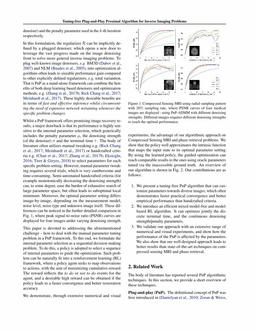
Whilst a PnP framework offers promising image recovery re-sults, a major drawback is that its performance is highly sen-sitive to the internal parameter selection, which genericallyincludes the penalty parameter µ, the denoising strength(of the denoiser) σ and the terminal time τ . The body ofliterature often utilizes manual tweaking e.g. (Rick Changet al., 2017; Meinhardt et al., 2017) or handcrafted crite-ria e.g. (Chan et al., 2017; Zhang et al., 2017b; Eksioglu,2016; Tirer & Giryes, 2018) to select parameters for eachspecific problem setting. However, manual parameter tweak-ing requires several trials, which is very cumbersome andtime-consuming. Semi-automated handcrafted criteria (forexample monotonically decreasing the denoising strength)can, to some degree, ease the burden of exhaustive search oflarge parameter space, but often leads to suboptimal localminimum. Moreover, the optimal parameter setting differsimage-by-image, depending on the measurement model,noise level, noise type and unknown image itself. These dif-ferences can be noticed in the further detailed comparison inFig. 1, where peak signal-to-noise ratio (PSNR) curves aredisplayed for four images under varying denoising strength.

This paper is devoted to addressing the aforementionedchallenge – how to deal with the manual parameter tuningproblem in a PnP framework. To this end, we formulate theinternal parameter selection as a sequential decision-makingproblem. To do this, a policy is adopted to select a sequenceof internal parameters to guide the optimization. Such prob-lem can be naturally fit into a reinforcement learning (RL)framework, where a policy agent seeks to map observationsto actions, with the aim of maximizing cumulative-reward.The reward reflects the to do or not to do events for theagent, and a desirable high reward can be obtained if thepolicy leads to a faster convergence and better restorationaccuracy.

We demonstrate, through extensive numerical and visual

Figure 1. Compressed Sensing MRI using radial sampling patternwith 20% sampling rate, where PSNR curves of four medicalimages are displayed - using PnP-ADMM with different denoisingstrengths. Different images requires different denoising strengthsto reach the optimal performance.

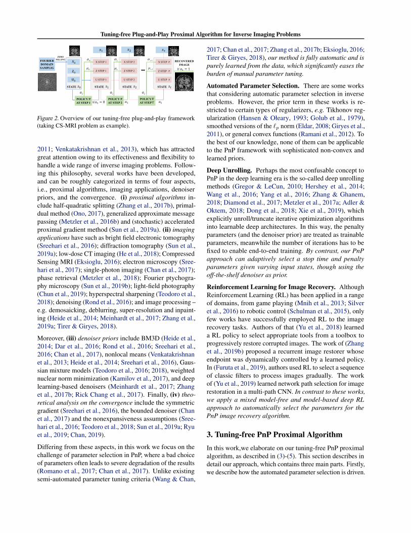
experiments, the advantage of our algorithmic approach onCompressed Sensing MRI and phase retrieval problems. Weshow that the policy well approximates the intrinsic functionthat maps the input state to its optimal parameter setting.By using the learned policy, the guided optimization canreach comparable results to the ones using oracle parameterstuned via the inaccessible ground truth. An overview ofour algorithm is shown in Fig. 2. Our contributions are asfollows:

1. We present a tuning-free PnP algorithm that can cus-tomize parameters towards diverse images, which oftendemonstrates faster practical convergence and betterempirical performance than handcrafted criteria.

2. We introduce an efficient mixed model-free and model-based RL algorithm. It can optimize jointly the dis-crete terminal time, and the continuous denoisingstrength/penalty parameters.

3. We validate our approach with an extensive range ofnumerical and visual experiments, and show how theperformance of the PnP is affected by the parameters.We also show that our well-designed approach leads tobetter results than state-of-the-art techniques on com-pressed sensing MRI and phase retrieval.

2. Related WorkThe body of literature has reported several PnP algorithmictechniques. In this section, we provide a short overview ofthese techniques.

Plug-and-play (PnP). The definitional concept of PnP wasfirst introduced in (Danielyan et al., 2010; Zoran & Weiss,


FOURIER DOMAIN SAMPLIG

ZEROFILLING

X STEP 1

Z STEP 1

U STEP 1

X STEP 2

Z STEP 2

U STEP 2

RECOVERED IMAGE

1-0 1

0 1 1-

X STEP

POLICYAT STEP 1

𝜋

0x

0u0z

𝑎 0

2a 2a 2a

U STEP

Z STEP

𝑠STATE

𝑥 𝑥 𝑥

𝑠STATE 𝑠STATE 𝑠STATE

If 𝑎 𝑎

𝑎 1If

POLICY AT STEP

𝜋𝜏

POLICY AT STEP 2

𝜋

Figure 2. Overview of our tuning-free plug-and-play framework(taking CS-MRI problem as example).

2011; Venkatakrishnan et al., 2013), which has attractedgreat attention owing to its effectiveness and flexibility tohandle a wide range of inverse imaging problems. Follow-ing this philosophy, several works have been developed,and can be roughly categorized in terms of four aspects,i.e., proximal algorithms, imaging applications, denoiserpriors, and the convergence. (i) proximal algorithms in-clude half-quadratic splitting (Zhang et al., 2017b), primal-dual method (Ono, 2017), generalized approximate messagepassing (Metzler et al., 2016b) and (stochastic) acceleratedproximal gradient method (Sun et al., 2019a). (ii) imagingapplications have such as bright field electronic tomography(Sreehari et al., 2016); diffraction tomography (Sun et al.,2019a); low-dose CT imaging (He et al., 2018); CompressedSensing MRI (Eksioglu, 2016); electron microscopy (Sree-hari et al., 2017); single-photon imaging (Chan et al., 2017);phase retrieval (Metzler et al., 2018); Fourier ptychogra-phy microscopy (Sun et al., 2019b); light-field photography(Chun et al., 2019); hyperspectral sharpening (Teodoro et al.,2018); denoising (Rond et al., 2016); and image processing –e.g. demosaicking, deblurring, super-resolution and inpaint-ing (Heide et al., 2014; Meinhardt et al., 2017; Zhang et al.,2019a; Tirer & Giryes, 2018).

Moreover, (iii) denoiser priors include BM3D (Heide et al.,2014; Dar et al., 2016; Rond et al., 2016; Sreehari et al.,2016; Chan et al., 2017), nonlocal means (Venkatakrishnanet al., 2013; Heide et al., 2014; Sreehari et al., 2016), Gaus-sian mixture models (Teodoro et al., 2016; 2018), weightednuclear norm minimization (Kamilov et al., 2017), and deeplearning-based denoisers (Meinhardt et al., 2017; Zhanget al., 2017b; Rick Chang et al., 2017). Finally, (iv) theo-retical analysis on the convergence include the symmetricgradient (Sreehari et al., 2016), the bounded denoiser (Chanet al., 2017) and the nonexpansiveness assumptions (Sree-hari et al., 2016; Teodoro et al., 2018; Sun et al., 2019a; Ryuet al., 2019; Chan, 2019).

Differing from these aspects, in this work we focus on thechallenge of parameter selection in PnP, where a bad choiceof parameters often leads to severe degradation of the results(Romano et al., 2017; Chan et al., 2017). Unlike existingsemi-automated parameter tuning criteria (Wang & Chan,

2017; Chan et al., 2017; Zhang et al., 2017b; Eksioglu, 2016;Tirer & Giryes, 2018), our method is fully automatic and ispurely learned from the data, which significantly eases theburden of manual parameter tuning.

Automated Parameter Selection. There are some worksthat considering automatic parameter selection in inverseproblems. However, the prior term in these works is re-stricted to certain types of regularizers, e.g. Tikhonov reg-ularization (Hansen & Ołeary, 1993; Golub et al., 1979),smoothed versions of the `p norm (Eldar, 2008; Giryes et al.,2011), or general convex functions (Ramani et al., 2012). Tothe best of our knowledge, none of them can be applicableto the PnP framework with sophisticated non-convex andlearned priors.

Deep Unrolling. Perhaps the most confusable concept toPnP in the deep learning era is the so-called deep unrollingmethods (Gregor & LeCun, 2010; Hershey et al., 2014;Wang et al., 2016; Yang et al., 2016; Zhang & Ghanem,2018; Diamond et al., 2017; Metzler et al., 2017a; Adler &Oktem, 2018; Dong et al., 2018; Xie et al., 2019), whichexplicitly unroll/truncate iterative optimization algorithmsinto learnable deep architectures. In this way, the penaltyparameters (and the denoiser prior) are treated as trainableparameters, meanwhile the number of iterations has to befixed to enable end-to-end training. By contrast, our PnPapproach can adaptively select a stop time and penaltyparameters given varying input states, though using theoff-the-shelf denoiser as prior.

Reinforcement Learning for Image Recovery. AlthoughReinforcement Learning (RL) has been applied in a rangeof domains, from game playing (Mnih et al., 2013; Silveret al., 2016) to robotic control (Schulman et al., 2015), onlyfew works have successfully employed RL to the imagerecovery tasks. Authors of that (Yu et al., 2018) learneda RL policy to select appropriate tools from a toolbox toprogressively restore corrupted images. The work of (Zhanget al., 2019b) proposed a recurrent image restorer whoseendpoint was dynamically controlled by a learned policy.In (Furuta et al., 2019), authors used RL to select a sequenceof classic filters to process images gradually. The workof (Yu et al., 2019) learned network path selection for imagerestoration in a multi-path CNN. In contrast to these works,we apply a mixed model-free and model-based deep RLapproach to automatically select the parameters for thePnP image recovery algorithm.

3. Tuning-free PnP Proximal AlgorithmIn this work,we elaborate on our tuning-free PnP proximalalgorithm, as described in (3)-(5). This section describes indetail our approach, which contains three main parts. Firstly,we describe how the automated parameter selection is driven.


Secondly, we introduce our environment model, and finally,we introduce the policy learning, which is guided by a mixedmodel-free and a model-based RL.

It is worth mentioning that our method is generic, and canbe applicable to PnP methods derived from other proximalalgorithms, e.g. forward backward splitting, as well. Thereason is that these are distinct methods, they share the samefixed points as PnP-ADMM (Meinhardt et al., 2017).

3.1. RL Formulation for Automated ParameterSelection

This work mainly focuses on the automated parameter selec-tion problem in the PnP framework, where we aim to selecta sequence of parameters (σ0, µ0, σ1, µ1, · · · , στ−1, µτ−1)to guide optimization such that the recovered image xτ isclose to the underlying image x. We formulate this prob-lem as a Markov decision process (MDP), which can beaddressed via reinforcement learning (RL).

We denote the MDP by the tuple (S,A, p, r), where S is thestate space,A is the action space, p is the transition functiondescribing the environment dynamics, and r is the rewardfunction. Specifically, for our task, S is the space of opti-mization variable states, which includes the initialization(x0, z0, u0) and all intermedia results (xk, zk, uk) in the op-timization process. A is the space of internal parameters,including both discrete terminal time τ and the continuousdenoising strength/penalty parameters (σk, µk). The transi-tion function p : S ×A 7→ S maps input state s ∈ S to itsoutcome state s′ ∈ S after taking action a ∈ A. The statetransition can be expressed as st+1 = p(st, at), which iscomposed of one or several iterations of optimization. Oneach transition, the environment emits a reward in terms ofthe reward function r : S×A 7→ R, which evaluates actionsgiven the state. Applying a sequence of parameters to theinitial state s0 results in a trajectory T of states, actionsand rewards: T = {s0, a0, r0, · · · , sN , aN , rN}. Given atrajectory T , we define the return rγt as the summation ofdiscounted rewards after st,

rγt =

N−t∑t′=0

γt′r(st+t′ , at+t′), (6)

where γ ∈ [0, 1] is a discount factor and prioritizes earlierrewards over later ones.

Our goal is to learn a policy π, denoted as π(a|s) : S 7→ Afor the decision-making agent, in order to maximize theobjective defined as

J (π) = Es0∼S0,T∼π [rγ0 ] , (7)

where E represents expectation, s0 is the initial state, andS0 is the corresponding initial state distribution. Intuitively,the objective describes the expected return over all possible

trajectories induced by the policy π. The expected return onstates and state-action pairs under the policy π are definedby state-value functions V π and action-value functions Qπ

respectively, i.e.,

V π (s) = ET∼π [rγ0 |s0 = s] , (8)Qπ (s, a) = ET∼π [rγ0 |s0 = s, a0 = a] . (9)

In our task, we decompose actions into two parts: a dis-crete decision a1 on terminal time and a continuous deci-sion a2 on denoising strength and penalty parameter. Thepolicy also consists of two sub-policies: π = (π1, π2), astochastic policy and a deterministic policy that generatea1 and a2 respectively. The role of π1 is to decide whetherto terminate the iterative algorithm when the next state isreached. It samples a boolean-valued outcome a1 from atwo-class categorical distribution π1(·|s), whose probabilitymass function is calculated from the current state s. Wemove forward to the next iteration if a1 = 0, otherwisethe optimization would be terminated to output the finalstate. Compared to the stochastic policy π1, we treat π2deterministically, i.e. a2 = π2(s) since π2 is differentiablewith respect to the environment, such that its gradient canbe precisely estimated.

3.2. Environment Model

In RL, the environment is characterized by two components:the environment dynamics and reward function. In our task,the environment dynamics is described by the transitionfunction p related to the PnP-ADMM. Here, we elucidatethe detailed setting of the PnP-ADMM as well as the rewardfunction used for training policy.

Denoiser Prior. Differentiable environment makes thepolicy learning more efficient. To make the environmentdifferentiable with respect to π21, we take a convolutionalneural network (CNN) denoiser as the image prior. In prac-tice, we use a residual U-Net (Ronneberger et al., 2015)architecture, which was originally designed for medical im-age segmentation, but was founded to be useful in imagedenoising recently. Besides, we incorporate an additionaltunable noise level map into the input as (Zhang et al., 2018),enabling us to provide continuous noise level control (i.e.different denoising strength) within a single network.

Proximal operator of data-fidelity term. Enforcing con-sistency with measured data requires evaluating the proxi-mal operator in (4). For inverse problems, there might existfast solutions due to the special structure of the observationmodel. We adopt the fast solution if feasible (e.g. closed-form solution using fast Fourier transform, rather than thegeneral matrix inversion) otherwise a single step of gradientdescent is performed as an inexact solution for (4).

1π1 is non-differentiable towards environment regardless of theformulation of the environment.


Transition function. To reduce the computation cost, wedefine the transition function p to involve m iterations ofthe optimization. At each time step, the agent thus needs todecide the internal parameters for m iterates. We set m = 5and the max time step N = 6 in our algorithm, leading to30 iterations of the optimization at most.

Reward function. To take both image recovery perfor-mance and runtime efficiency into account, we define thereward function as

r(st, at) = ζ(p(st, at))− ζ(st)− η. (10)

The first term, ζ(p(st, at))−ζ(st), denotes the PSNR incre-ment made by the policy, where ζ(st) denotes the PSNR ofthe recovered image at step t. A higher reward is acquiredif the policy leads to higher performance gain in terms ofPSNR. The second term, η, implies penalizing the policyas it does not select to terminate at step t, where η sets thedegree of penalty. A negative reward is given if the PSNRgain does not exceed the degree of penalty, thereby encour-aging the policy to early stop the iteration with diminishedreturn. We set η = 0.05 in our algorithm2.

3.3. RL-based policy learning

In this section, we present a mixed model-free and model-based RL algorithm to learn the policy. Specifically, model-free RL (agnostic to the environment dynamics) is usedto train π1, while model-based RL is utilized to optimizeπ2 to make full use of the environment model3. We ap-ply the actor-critic framework (Sutton et al., 2000), thatuses a policy network πθ(at|st) (actor) and a value networkV πφ (st) (critic) to formulate the policy and the state-valuefunction respectively4. The policy and the value networksare learned in an interleaved manner. For each gradient step,we optimize the value network parameters φ by minimizing

Lφ = Es∼D,a∼πθ(s)[1

2(r(s, a) + γV π

φ̂(p(s, a))− V πφ (s))2

],

(11)

where D is the distribution of previously sampled states,practically implemented by a state buffer. This partly servesas a role of the experience replay mechanism (Lin, 1992),which is observed to ”smooth” the training data distribution(Mnih et al., 2013). The update makes use of a target valuenetwork V π

φ̂, where φ̂ is the exponentially moving average

of the value network weights and has been shown to stabilizetraining (Mnih et al., 2015).

2The choice of the hyperparameters m,N and η is discussedin the suppl. material.

3π2 can also be optimized in a model-free manner. The com-parison can be found in the Section 4.2.

4Details of networks are given in the suppl. material.

Table 1. Comparisons of different CNN-based denoisers: we showthe results of (1) Gaussian denoising performance (PSNR) un-der noise level σ = 50; (2) the CS-MRI performance (PSNR)when plugged into the PnP-ADMM; (3) the GPU runtime (ms) ofdenoisers when processing an image with size 256× 256.

Performance DnCNN MemNet UNetDENOISING PERF. 27.18 27.32 27.40

PNP PERF. 25.43 25.67 25.76TIMES 8.09 64.65 5.65

The policy network has two sub-policies, which employsshared convolutional layers to extract image features, fol-lowed by two separated groups of fully-connected layersto produce termination probability π1(·|s) (after softmax)or denoising strength/penalty parameters π2(s) (after sig-moid). We denote the parameters of the sub-polices as θ1and θ2 respectively, and we seek to optimize θ = (θ1, θ2)so that the objective J(πθ) is maximized. The policy net-work is trained using policy gradient methods (Peters &Schaal, 2006). The gradient of θ1 is estimated in a model-free manner by a likelihood estimator, while the gradientof θ2 is estimated relying on backpropagation via environ-ment dynamics in a model-based manner. Specifically, fordiscrete terminal time decision π1, we apply the policygradient theorem (Sutton et al., 2000) to obtain unbiasedMonte Carlo estimate of Oθ1J(πθ) using advantage func-tion Aπ(s, a) = Qπ(s, a)− V π(s) as target, i.e.,

Oθ1J(πθ) =Es∼D,a∼πθ(s) [Oθ1 log π1(a1|s)Aπ(s, a)] .

(12)

For continuous denoising strength and penalty parameterselection π2, we utilize the deterministic policy gradienttheorem (Silver et al., 2014) to formulate its gradient, i.e.,

Oθ2J(πθ) =Es∼D,a∼πθ(s) [Oa2 Qπ(s, a)Oθ2π2(s)] ,

(13)

where we approximate the action-value function Qπ(s, a)by r(s, a) + γV πφ (p(s, a)) given its unfolded definition.

Using the chain rule, we can directly obtain the gradient ofθ2 by backpropagation via the reward function, the valuenetwork and the transition function, in contrast to relying onthe gradient backpropagated from only the learned action-value function in the model-free DDPG algorithm (Lillicrapet al., 2016).

4. ExperimentsIn this section, we detail the experiments and evaluate ourproposed algorithm. We mainly focus on the tasks of Com-pressed Sensing MRI (CS-MRI) and phase retrieval (PR),which are the representative linear and nonlinear inverseimaging problems respectively.


Table 2. Comparisons of different policies used in PnP-ADMMalgorithm for CS-MRI on seven widely used medical images undervarious acceleration factors (x2/x4/x8) and noise level 15. Weshow both PSNR and the number of iterations (#IT.) used to induceresults. * denotes to report the best PSNR over all iterations (i.e.with optimal early stopping). The best results are indicated byorange color and the second best results are denoted by blue color.

×2 ×4 ×8POLICIES PSNR #IT. PSNR #IT. PSNR #IT.

handcrafted 30.05 30.0 27.90 30.0 25.76 30.0handcrafted∗ 30.06 29.1 28.20 18.4 26.06 19.4fixed 23.94 30.0 24.26 30.0 22.78 30.0fixed∗ 28.45 1.6 26.67 3.4 24.19 7.3fixed optimal 30.02 30.0 28.27 30.0 26.08 16.7fixed optimal∗ 30.03 6.7 28.34 12.6 26.16 30.0oracle 30.25 30.0 28.60 30.0 26.41 30.0oracle∗ 30.26 8.0 28.61 13.9 26.45 21.6

model-free 28.79 30.0 27.95 30.0 26.15 30.0Ours 30.33 5.0 28.42 5.0 26.44 15.0

4.1. Implementation Details

Our algorithm requires two training processes for: the de-noising network and the policy network (and value network).For training the denoising network, we follow the commonpractice that uses 87,000 overlapping patches (with size128× 128) drawn from 400 images from the BSD dataset(Martin et al., 2001). For each patch, we add white Gaussiannoise with noise level sampled from [1, 50]. The denoisingnetworks are trained with 50 epoch using L1 loss and Adamoptimizer (Kingma & Ba, 2014) with batch size 32. Thebase learning rate is set to 10−4 and halved at epoch 30,then reduced to 10−5 at epoch 40.

To train the policy network and value network, we use the17,125 resized images with size 128×128 from the PASCALVOC dataset (Everingham et al., 2014). Both networks aretrained using Adam optimizer with batch size 48 and 1500iterations, with a base learning rate of 3 × 10−4 for thepolicy network and 10−3 for the value network. Then weset these learning rates to 10−4 and 3 × 10−4 at iteration1000. We perform 10 gradient steps at every iteration.

For the CS-MRI application, a single policy network istrained to handle multiple sampling ratios (with x2/x4/x8acceleration) and noise levels (5/10/15), simultaneously.Similarly, one policy network is learned for phase retrievalunder different settings.

4.2. Compressed sensing MRI

The forward model of CS-MRI can be mathematicallydescribed as y = Fpx + ω, where x ∈ CN is the un-derlying image, the operator Fp : CN → CM , withM < N , denotes the partially-sampled Fourier transform,and ω ∼ N (0, σnIM ) is the additive white Gaussian noise.The data-fidelity term is D(x) = 1

2‖y−Fpx‖2 whose prox-

imal operator is given in (Eksioglu, 2016).

Denoiser priors. To show how denoiser priors affect theperformance of the PnP, we train three state-of-the-art CNN-based denoisers, i.e. DnCNN (Zhang et al., 2017a), Mem-Net (Tai et al., 2017) and residual UNet (Ronneberger et al.,2015), with tunable noise level map. We compare both theGaussian denoising performance and the PnP performance5

using these denoisers. As shown in Table 1, the resid-ual UNet and MemNet consistently outperform DnCNNin terms of denoising and CS-MRI. It seems to imply abetter Gaussian denoiser is also a better denoiser prior forthe PnP framework6. Since UNet is significantly faster thanMemNet, we choose UNet as our denoiser prior.

Comparisons of different policies. We start by givingsome insights of our learned policy by comparing the per-formance of PnP-ADMM with different polices: i) the hand-crafted policy used in IRCNN (Zhang et al., 2017b); ii) thefixed policy that uses fixed parameters (σ = 15, µ = 0.1);iii) the fixed optimal policy that adopts fixed parameterssearched to maximize the average PSNR across all testingimages; iv) the oracle policy that uses different parametersfor different images such that the PSNR of each image ismaximized and v) our learned policy based on a learnedpolicy network to optimize parameters for each image. Weremark that all compared polices are run for 30 iterationwhilst ours automatically choose the terminal time.

To understand the usefulness of the early stopping mecha-nism, we also report the results of these polices with optimalearly stopping7. Moreover, we analyze whether the model-based RL benefits our algorithm by comparing it with thelearned policy by model-free RL whose π2 is optimized us-ing the model-free DDPG algorithm (Lillicrap et al., 2016).

The results of all aforementioned policies are provided inTable 2. We can see that the bad choice of parameters (see“fixed”) induces poor results, in which the early stopping isquite needed to rescue performance (see “fixed∗”). Whenthe parameters are properly assigned, the early stoppingwould be helpful to reduce computation cost. Our learnedpolicy leads to fast practical convergence as well as excellentperformance, sometimes even outperforms the oracle policytuned via inaccessible ground truth (in ×2 case). We notethis is owing to the varying parameters across iterationsgenerated automatically in our algorithm, which yield extraflexibility than constant parameters over iterations. Besides,we find the learned model-free policy produces suboptimal

5We exhaustively search the best denoising strength/penaltyparameters to exclude the impact of internal parameters.

6Further investigation of this argument can be found in thesuppl. material.

7It should be noted some policies (e.g. ”fixed optimal” and ”or-acle”) requires to access the ground truth to determine parameters,which is generally impractical in real testing scenarios.


Table 3. Quantitative results (PSNR) of different CS-MRI methods on two datasets under various acceleration factors f and noise levelsσn. The best results are indicated by orange color and the second best results are denoted by blue color.

DATASET f σnTRADITIONAL DEEP UNROLLING PNP

RecPF FCSA ADMMNet ISTANet BM3D-MRI IRCNN Ours

Medical7

×25 32.46 31.70 33.10 34.58 33.33 34.67 34.7810 29.48 28.33 31.37 31.81 29.44 31.80 32.0015 27.08 25.52 29.16 29.99 26.90 29.96 30.27

×45 28.67 28.21 30.24 31.34 30.33 31.36 31.6210 26.98 26.67 29.20 29.71 28.30 29.52 29.6815 25.58 24.93 27.87 28.38 26.66 27.94 28.43

×85 24.72 24.62 26.57 27.65 26.53 27.32 28.2610 23.94 24.04 26.21 26.90 25.81 26.44 27.3515 23.18 23.36 25.49 26.23 25.09 25.53 26.41

MICCAI

×25 36.39 34.90 36.74 38.17 36.00 38.42 38.5710 31.95 30.12 34.20 34.81 31.39 34.93 35.0615 28.91 26.68 31.42 32.65 28.46 32.81 33.09

×45 33.05 32.30 34.15 35.46 34.79 35.80 36.1110 30.21 29.56 32.58 33.13 31.63 32.99 33.0715 28.13 26.93 30.55 31.48 29.35 30.98 31.42

×85 28.35 28.71 30.36 31.62 31.34 31.66 32.6410 26.86 27.68 29.78 30.54 29.86 30.16 30.8915 25.70 26.35 28.83 29.50 28.53 28.72 29.65

Table 4. Quantitative results of different PR algorithms on fourCDP measurements and varying amount of Possion noise (large αindicates low sigma-to-noise ratio).

α = 9 α = 27 α = 81Algorithms PSNR PSNR PSNR

HIO 35.96 25.76 14.82WF 34.46 24.96 15.76DOLPHIn 29.93 27.45 19.35SPAR 35.20 31.82 22.44BM3D-prGAMP 40.25 32.84 25.43prDeep 39.70 33.54 26.82Ours 40.33 33.90 27.23

denoising strength/penalty parameters compared with ourmixed model-free and model-based policy, and it also failsto learn early stopping behavior.

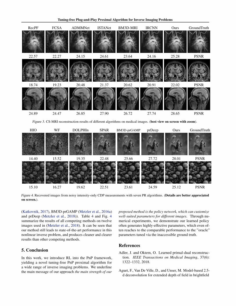
Comparisons with state-of-the-arts. We compare ourmethod against six state-of-the-art methods for CS-MRI,including the traditional optimization-based approaches(RecPF (Yang et al., 2010) and FCSA (Huang et al., 2010)),the PnP approaches (BM3D-MRI (Eksioglu, 2016) and IR-CNN (Zhang et al., 2017b)), and the deep unrolling ap-proaches (ADMMNet (Yang et al., 2016) and ISTANet(Zhang & Ghanem, 2018)). To keep comparison fair, foreach deep unrolling method, only single network is trainedto tackle all the cases using the same dataset as ours. Table3 shows the method performance on two set of medical im-ages, i.e. 7 widely used medical images (Medical7) (Huanget al., 2010) and 50 medical images from MICCAI 2013grand challenge dataset8. The visual comparison can be

8https://my.vanderbilt.edu/masi/

found in Fig. 3. It can be seen that our approach significantlyoutperforms the state-of-the-art PnP method (IRCNN) bya large margin, especially under the difficult ×8 case. Inthe simple cases (e.g. ×2), our algorithm only runs 5 it-erations to arrive at the desirable performance, in contrastwith 30 or 70 iterations required in IRCNN and BM3D-MRIrespectively.

4.3. Phase retrieval

The goal of phase retrieval (PR) is to recover the underlyingimage from only the amplitude, or intensity of the outputof a complex linear system. Mathematically, PR can bedefined as the problem of recovering a signal x ∈ RN orCN from measurement y of the form y = |Ax|+ ω, wherethe measurement matrix A represents the forward operatorof the system, and ω represents shot noise. We approximateit with ω ∼ N (0, α|Ax|). The term α controls the sigma-to-noise ratio in this problem.

We test algorithms with coded diffraction pattern (CDP)(Cands et al., 2015). Multiple measurements, with differentrandom spatial modulator (SLM) patterns are recorded. Wemodel the capture of four measurements using a phase-onlySLM as (Metzler et al., 2018). Each measurement opera-tor can be mathematically described as Ai = FDi, i ∈[1, 2, 3, 4], where F can be represented by the 2D Fouriertransform and Di is diagonal matrices with nonzero ele-ments drawn uniformly from the unit circle in the complexplanes.

We compare our method with three classic approaches (HIO(Fienup, 1982), WF (Candes et al., 2014), and DOLPHIn(Mairal et al., 2016)) and three PnP approaches (SPAR


RecPF FCSA ADMMNet ISTANet BM3D-MRI IRCNN Ours GroundTruth

22.57 22.27 24.15 24.61 23.64 24.16 25.28 PSNR

18.74 19.23 20.48 21.37 20.62 20.91 22.02 PSNR

24.89 24.47 26.85 27.90 26.72 27.74 28.65 PSNR

Figure 3. CS-MRI reconstruction results of different algorithms on medical images. (best view on screen with zoom).

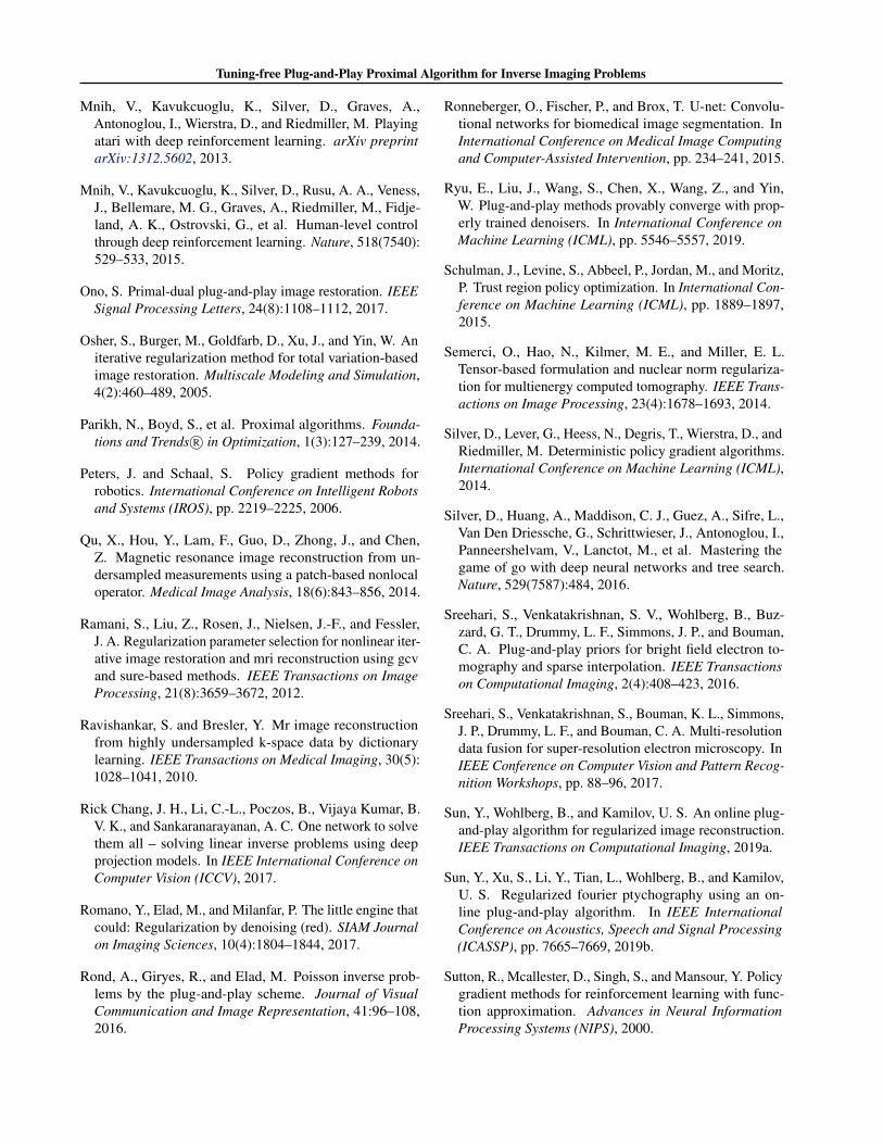
HIO WF DOLPHIn SPAR BM3D-prGAMP prDeep Ours GroundTruth

14.40 15.52 19.35 22.48 25.66 27.72 28.01 PSNR

15.10 16.27 19.62 22.51 23.61 24.59 25.12 PSNR

Figure 4. Recovered images from noisy intensity-only CDP measurements with seven PR algorithms. (Details are better appreciatedon screen.).

(Katkovnik, 2017), BM3D-prGAMP (Metzler et al., 2016a)and prDeep (Metzler et al., 2018)). Table 4 and Fig. 4summarize the results of all competing methods on twelveimages used in (Metzler et al., 2018). It can be seen thatour method still leads to state-of-the-art performance in thisnonlinear inverse problem, and produces cleaner and clearerresults than other competing methods.

5. ConclusionIn this work, we introduce RL into the PnP framework,yielding a novel tuning-free PnP proximal algorithm fora wide range of inverse imaging problems. We underlinethe main message of our approach the main strength of our

proposed method is the policy network, which can customizewell-suited parameters for different images. Through nu-merical experiments, we demonstrate our learned policyoften generates highly-effective parameters, which even of-ten reaches to the comparable performance to the ”oracle”parameters tuned via the inaccessible ground truth.

ReferencesAdler, J. and Oktem, O. Learned primal-dual reconstruc-

tion. IEEE Transactions on Medical Imaging, 37(6):1322–1332, 2018.

Aguet, F., Van De Ville, D., and Unser, M. Model-based 2.5-d deconvolution for extended depth of field in brightfield


microscopy. IEEE Transactions on Image Processing, 17(7):1144–1153, 2008.

Beck, A. and Teboulle, M. A fast iterative shrinkage-thresholding algorithm for linear inverse problems. SIAMJournal on Imaging Sciences, 2(1):183–202, 2009.

Boyd, S., Parikh, N., Chu, E., Peleato, B., Eckstein, J., et al.Distributed optimization and statistical learning via thealternating direction method of multipliers. Foundationsand Trends R© in Machine learning, 3(1):1–122, 2011.

Buades, A., Coll, B., and Morel, J.-M. A non-local al-gorithm for image denoising. In IEEE Conference onComputer Vision and Pattern Recognition (CVPR), pp.60–65, 2005.

Candes, E., Li, X., and Soltanolkotabi, M. Phase retrievalvia wirtinger flow: Theory and algorithms. IEEE Trans-actions on Information Theory, 61, 07 2014.

Cands, E. J., Li, X., and Soltanolkotabi, M. Phase retrievalfrom coded diffraction patterns. Applied and Computa-tional Harmonic Analysis, 39(2):277–299, 2015.

Chambolle, A. and Pock, T. A first-order primal-dual algo-rithm for convex problems with applications to imaging.Journal of Mathematical Imaging and Vision, 40(1):120–145, 2011.

Chan, S. H. Performance analysis of plug-and-play admm:A graph signal processing perspective. IEEE Transactionson Computational Imaging, 5(2):274–286, 2019.

Chan, S. H., Wang, X., and Elgendy, O. A. Plug-and-playadmm for image restoration: Fixed-point convergenceand applications. IEEE Transactions on ComputationalImaging, 3(1):84–98, 2017.

Chun, I. Y., Huang, Z., Lim, H., and Fessler, J. A.Momentum-net: Fast and convergent iterative neu-ral network for inverse problems. arXiv preprintarXiv:1907.11818, 2019.

Dabov, K., Foi, A., Katkovnik, V., and Egiazarian, K. Imagedenoising by sparse 3-d transform-domain collaborativefiltering. IEEE Transactions on Image Processing, 16(8):2080, 2007.

Danielyan, A., Katkovnik, V., and Egiazarian, K. Imagedeblurring by augmented lagrangian with bm3d frameprior. In Workshop on Information Theoretic Methods inScience and Engineering, pp. 16–18, 2010.

Dar, Y., Bruckstein, A. M., Elad, M., and Giryes, R. Postpro-cessing of compressed images via sequential denoising.IEEE Transactions on Image Processing, 25(7):3044–3058, 2016.

Diamond, S., Sitzmann, V., Heide, F., and Wetzstein, G.Unrolled optimization with deep priors. arXiv preprintarXiv:1705.08041, 2017.

Dong, W., Wang, P., Yin, W., Shi, G., Wu, F., and Lu, X.Denoising prior driven deep neural network for imagerestoration. IEEE Transactions on Pattern Analysis andMachine Intelligence, 41(10):2305–2318, 2018.

Eksioglu, E. M. Decoupled algorithm for mri reconstructionusing nonlocal block matching model: Bm3d-mri. Jour-nal of Mathematical Imaging and Vision, 56(3):430–440,2016.

Elbakri, I. A. and Fessler, J. A. Segmentation-free statis-tical image reconstruction for polyenergetic x-ray com-puted tomography. In IEEE International Symposium onBiomedical Imaging, pp. 828–831, 2002.

Eldar, Y. C. Generalized sure for exponential families: Ap-plications to regularization. IEEE Transactions on SignalProcessing, 57(2):471–481, 2008.

Esser, E., Zhang, X., and Chan, T. F. A general frameworkfor a class of first order primal-dual algorithms for con-vex optimization in imaging science. SIAM Journal onImaging Sciences, 3(4):1015–1046, 2010.

Everingham, M., Eslami, S., Van Gool, L., Williams, C.,Winn, J., and Zisserman, A. The pascal visual objectclasses challenge: A retrospective. International Journalof Computer Vision, 111, 01 2014.

Fessler, J. A. Model-based image reconstruction for mri.IEEE Signal Processing Magazine, 27(4):81–89, 2010.

Fienup, J. R. Phase retrieval algorithms: a comparison.Applied Optics, 21(15):2758–2769, 1982.

Furuta, R., Inoue, N., and Yamasaki, T. Fully convolutionalnetwork with multi-step reinforcement learning for imageprocessing. In AAAI Conference on Artificial Intelligence,pp. 3598–3605, 2019.

Geman, D. Nonlinear image recovery with half-quadraticregularization. IEEE Transactions on Image Processing,4(7):932–946, 1995.

Giryes, R., Elad, M., and Eldar, Y. C. The projected gsure forautomatic parameter tuning in iterative shrinkage meth-ods. Applied and Computational Harmonic Analysis, 30(3):407–422, 2011.

Golub, G. H., Heath, M., and Wahba, G. Generalized cross-validation as a method for choosing a good ridge parame-ter. Technometrics, 21(2):215–223, 1979.

http://arxiv.org/abs/1907.11818



Gregor, K. and LeCun, Y. Learning fast approximations ofsparse coding. In International Conference on MachineLearning (ICML), pp. 399–406, 2010.

Gu, S., Xie, Q., Meng, D., Zuo, W., Feng, X., and Zhang, L.Weighted nuclear norm minimization and its applicationsto low level vision. International Journal of ComputerVision, 121(2):183–208, 2017.

Hansen, P. C. and Ołeary, D. P. The use of the l-curve inthe regularization of discrete ill-posed problems. SIAMJournal on Scientific Computing, 14(6):1487–1503, 1993.

He, J., Yang, Y., Wang, Y., Zeng, D., Bian, Z., Zhang, H.,Sun, J., Xu, Z., and Ma, J. Optimizing a parameterizedplug-and-play admm for iterative low-dose ct reconstruc-tion. IEEE Transactions on Medical Imaging, 38(2):371–382, 2018.

Heide, F., Steinberger, M., Tsai, Y.-T., Rouf, M., Pajak, D.,Reddy, D., Gallo, O., Liu, J., Heidrich, W., Egiazarian,K., et al. Flexisp: A flexible camera image processingframework. ACM Transactions on Graphics, 33(6):231,2014.

Hershey, J. R., Roux, J. L., and Weninger, F. Deep unfold-ing: Model-based inspiration of novel deep architectures.arXiv preprint arXiv:1409.2574, 2014.

Huang, J., Zhang, S., and Metaxas, D. Efficient mr image re-construction for compressed mr imaging. Medical ImageAnalysis, 15:135–142, 2010.

Kamilov, U. S., Mansour, H., and Wohlberg, B. A plug-and-play priors approach for solving nonlinear imaginginverse problems. IEEE Signal Processing Letters, 24(12):1872–1876, 2017.

Katkovnik, V. Phase retrieval from noisy data based onsparse approximation of object phase and amplitude.arXiv preprint arXiv:1709.01071, 2017.

Katz, O., Heidmann, P., Fink, M., and Gigan, S. Non-invasive single-shot imaging through scattering layersand around corners via speckle correlations. Nature Pho-tonics, 8(10):784, 2014.

Kingma, D. P. and Ba, J. Adam: A method for stochasticoptimization. arXiv preprint arXiv:1412.6980, 2014.

Liao, H. Y. and Sapiro, G. Sparse representations for limiteddata tomography. In IEEE International Symposium onBiomedical Imaging: From Nano to Macro, pp. 1375–1378. IEEE, 2008.

Lillicrap, T., Hunt, J. J., Pritzel, A., Heess, N., Erez, T.,Tassa, Y., Silver, D., and Wierstra, D. Continuous controlwith deep reinforcement learning. international confer-ence on learning representations (ICLR), 2016.

Lin, L. Self-improving reactive agents based on reinforce-ment learning, planning and teaching. Machine Learning,8(3):293–321, 1992.

Ma, S., Yin, W., Zhang, Y., and Chakraborty, A. An effi-cient algorithm for compressed mr imaging using totalvariation and wavelets. In IEEE Conference on ComputerVision and Pattern Recognition (CVPR), pp. 1–8. IEEE,2008.

Mairal, Julien, Tillmann, Andreas, M., Eldar, Yonina, andC. Dolphin-dictionary learning for phase retrieval. IEEETransactions on Signal Processing, 2016.

Mairal, J., Bach, F. R., Ponce, J., Sapiro, G., and Zisser-man, A. Non-local sparse models for image restoration.In IEEE International Conference on Computer Vision(ICCV), volume 29, pp. 54–62, 2009.

Martin, D., Fowlkes, C., Tal, D., and Malik, J. A databaseof human segmented natural images and its applicationto evaluating segmentation algorithms and measuringecological statistics. In IEEE International Conferenceon Computer Vision (ICCV), pp. 416–423, 2001.

Meinhardt, T., Moller, M., Hazirbas, C., and Cremers, D.Learning proximal operators: Using denoising networksfor regularizing inverse imaging problems. In IEEE In-ternational Conference on Computer Vision (ICCV), Oct2017.

Metzler, C., Mousavi, A., and Baraniuk, R. Learned d-amp: Principled neural network based compressive imagerecovery. In Advances in Neural Information ProcessingSystems (NIPS), pp. 1772–1783. 2017a.

Metzler, C., Schniter, P., Veeraraghavan, A., et al. prdeep:Robust phase retrieval with a flexible deep network. InInternational Conference on Machine Learning (ICML),pp. 3498–3507, 2018.

Metzler, C. A., Maleki, A., and Baraniuk, R. G. Bm3d-prgamp: Compressive phase retrieval based on bm3ddenoising. In IEEE International Conference on ImageProcessing, 2016a.

Metzler, C. A., Maleki, A., and Baraniuk, R. G. Fromdenoising to compressed sensing. IEEE Transactions onInformation Theory, 62(9):5117–5144, 2016b.

Metzler, C. A., Sharma, M. K., Nagesh, S., Baraniuk, R. G.,Cossairt, O., and Veeraraghavan, A. Coherent inversescattering via transmission matrices: Efficient phase re-trieval algorithms and a public dataset. In IEEE In-ternational Conference on Computational Photography(ICCP), pp. 1–16, 2017b.





Mnih, V., Kavukcuoglu, K., Silver, D., Graves, A.,Antonoglou, I., Wierstra, D., and Riedmiller, M. Playingatari with deep reinforcement learning. arXiv preprintarXiv:1312.5602, 2013.

Mnih, V., Kavukcuoglu, K., Silver, D., Rusu, A. A., Veness,J., Bellemare, M. G., Graves, A., Riedmiller, M., Fidje-land, A. K., Ostrovski, G., et al. Human-level controlthrough deep reinforcement learning. Nature, 518(7540):529–533, 2015.

Ono, S. Primal-dual plug-and-play image restoration. IEEESignal Processing Letters, 24(8):1108–1112, 2017.

Osher, S., Burger, M., Goldfarb, D., Xu, J., and Yin, W. Aniterative regularization method for total variation-basedimage restoration. Multiscale Modeling and Simulation,4(2):460–489, 2005.

Parikh, N., Boyd, S., et al. Proximal algorithms. Founda-tions and Trends R© in Optimization, 1(3):127–239, 2014.

Peters, J. and Schaal, S. Policy gradient methods forrobotics. International Conference on Intelligent Robotsand Systems (IROS), pp. 2219–2225, 2006.

Qu, X., Hou, Y., Lam, F., Guo, D., Zhong, J., and Chen,Z. Magnetic resonance image reconstruction from un-dersampled measurements using a patch-based nonlocaloperator. Medical Image Analysis, 18(6):843–856, 2014.

Ramani, S., Liu, Z., Rosen, J., Nielsen, J.-F., and Fessler,J. A. Regularization parameter selection for nonlinear iter-ative image restoration and mri reconstruction using gcvand sure-based methods. IEEE Transactions on ImageProcessing, 21(8):3659–3672, 2012.

Ravishankar, S. and Bresler, Y. Mr image reconstructionfrom highly undersampled k-space data by dictionarylearning. IEEE Transactions on Medical Imaging, 30(5):1028–1041, 2010.

Rick Chang, J. H., Li, C.-L., Poczos, B., Vijaya Kumar, B.V. K., and Sankaranarayanan, A. C. One network to solvethem all – solving linear inverse problems using deepprojection models. In IEEE International Conference onComputer Vision (ICCV), 2017.

Romano, Y., Elad, M., and Milanfar, P. The little engine thatcould: Regularization by denoising (red). SIAM Journalon Imaging Sciences, 10(4):1804–1844, 2017.

Rond, A., Giryes, R., and Elad, M. Poisson inverse prob-lems by the plug-and-play scheme. Journal of VisualCommunication and Image Representation, 41:96–108,2016.

Ronneberger, O., Fischer, P., and Brox, T. U-net: Convolu-tional networks for biomedical image segmentation. InInternational Conference on Medical Image Computingand Computer-Assisted Intervention, pp. 234–241, 2015.

Ryu, E., Liu, J., Wang, S., Chen, X., Wang, Z., and Yin,W. Plug-and-play methods provably converge with prop-erly trained denoisers. In International Conference onMachine Learning (ICML), pp. 5546–5557, 2019.

Schulman, J., Levine, S., Abbeel, P., Jordan, M., and Moritz,P. Trust region policy optimization. In International Con-ference on Machine Learning (ICML), pp. 1889–1897,2015.

Semerci, O., Hao, N., Kilmer, M. E., and Miller, E. L.Tensor-based formulation and nuclear norm regulariza-tion for multienergy computed tomography. IEEE Trans-actions on Image Processing, 23(4):1678–1693, 2014.

Silver, D., Lever, G., Heess, N., Degris, T., Wierstra, D., andRiedmiller, M. Deterministic policy gradient algorithms.International Conference on Machine Learning (ICML),2014.

Silver, D., Huang, A., Maddison, C. J., Guez, A., Sifre, L.,Van Den Driessche, G., Schrittwieser, J., Antonoglou, I.,Panneershelvam, V., Lanctot, M., et al. Mastering thegame of go with deep neural networks and tree search.Nature, 529(7587):484, 2016.

Sreehari, S., Venkatakrishnan, S. V., Wohlberg, B., Buz-zard, G. T., Drummy, L. F., Simmons, J. P., and Bouman,C. A. Plug-and-play priors for bright field electron to-mography and sparse interpolation. IEEE Transactionson Computational Imaging, 2(4):408–423, 2016.

Sreehari, S., Venkatakrishnan, S., Bouman, K. L., Simmons,J. P., Drummy, L. F., and Bouman, C. A. Multi-resolutiondata fusion for super-resolution electron microscopy. InIEEE Conference on Computer Vision and Pattern Recog-nition Workshops, pp. 88–96, 2017.

Sun, Y., Wohlberg, B., and Kamilov, U. S. An online plug-and-play algorithm for regularized image reconstruction.IEEE Transactions on Computational Imaging, 2019a.

Sun, Y., Xu, S., Li, Y., Tian, L., Wohlberg, B., and Kamilov,U. S. Regularized fourier ptychography using an on-line plug-and-play algorithm. In IEEE InternationalConference on Acoustics, Speech and Signal Processing(ICASSP), pp. 7665–7669, 2019b.

Sutton, R., Mcallester, D., Singh, S., and Mansour, Y. Policygradient methods for reinforcement learning with func-tion approximation. Advances in Neural InformationProcessing Systems (NIPS), 2000.



Tai, Y., Yang, J., Liu, X., and Xu, C. Memnet: A persistentmemory network for image restoration. In IEEE Inter-national Conference on Computer Vision (ICCV), Oct2017.

Teodoro, A. M., Bioucas-Dias, J. M., and Figueiredo, M. A.Image restoration and reconstruction using variable split-ting and class-adapted image priors. In IEEE Interna-tional Conference on Image Processing, pp. 3518–3522,2016.

Teodoro, A. M., Bioucas-Dias, J. M., and Figueiredo, M. A.A convergent image fusion algorithm using scene-adaptedgaussian-mixture-based denoising. IEEE Transactionson Image Processing, 28(1):451–463, 2018.

Tirer, T. and Giryes, R. Image restoration by iterative de-noising and backward projections. IEEE Transactions onImage Processing, 28(3):1220–1234, 2018.

Venkatakrishnan, S. V., Bouman, C. A., and Wohlberg, B.Plug-and-play priors for model based reconstruction. InIEEE Global Conference on Signal and Information Pro-cessing, pp. 945–948, 2013.

Wang, S., Fidler, S., and Urtasun, R. Proximal deep struc-tured models. In Advances in Neural Information Pro-cessing Systems (NIPS), pp. 865–873, 2016.

Wang, X. and Chan, S. H. Parameter-free plug-and-playadmm for image restoration. In IEEE InternationalConference on Acoustics, Speech and Signal Processing(ICASSP), pp. 1323–1327, 2017.

Xie, X., Wu, J., Liu, G., Zhong, Z., and Lin, Z. Differen-tiable linearized admm. In International Conference onMachine Learning (ICML), pp. 6902–6911, 2019.

Yang, J., Zhang, Y., and Yin, W. A fast alternating direc-tion method for tvl1-l2 signal reconstruction from partialfourier data. IEEE Journal of Selected Topics in SignalProcessing, 4(2):288–297, 2010.

Yang, Y., Sun, J., Li, H., and Xu, Z. Deep admm-net forcompressive sensing mri. In Advances in Neural Infor-mation Processing Systems (NIPS), pp. 10–18. 2016.

Yu, K., Dong, C., Lin, L., and Change Loy, C. Craftinga toolchain for image restoration by deep reinforcementlearning. In IEEE Conference on Computer Vision andPattern Recognition (CVPR), pp. 2443–2452, 2018.

Yu, K., Wang, X., Dong, C., Tang, X., and Loy, C. C.Path-restore: Learning network path selection for imagerestoration. arXiv preprint arXiv:1904.10343, 2019.

Zhang, J. and Ghanem, B. Ista-net: Interpretableoptimization-inspired deep network for image compres-sive sensing. In IEEE Conference on Computer Visionand Pattern Recognition (CVPR), 2018.

Zhang, K., Zuo, W., Chen, Y., Meng, D., and Zhang, L.Beyond a gaussian denoiser: Residual learning of deepcnn for image denoising. IEEE Transactions on ImageProcessing, 26(7):3142–3155, 2017a.

Zhang, K., Zuo, W., Gu, S., and Zhang, L. Learning deepcnn denoiser prior for image restoration. In IEEE Con-ference on Computer Vision and Pattern Recognition(CVPR), 2017b.

Zhang, K., Zuo, W., and Zhang, L. Ffdnet: Toward afast and flexible solution for cnn-based image denoising.IEEE Transactions on Image Processing, 27(9):4608–4622, 2018.

Zhang, K., Zuo, W., and Zhang, L. Deep plug-and-playsuper-resolution for arbitrary blur kernels. In IEEE Con-ference on Computer Vision and Pattern Recognition(CVPR), 2019a.

Zhang, X., Lu, Y., Liu, J., and Dong, B. Dynamically un-folding recurrent restorer: A moving endpoint controlmethod for image restoration. In International Confer-ence on Learning Representations (ICLR), 2019b.

Zheng, G., Horstmeyer, R., and Yang, C. Wide-field, high-resolution fourier ptychographic microscopy. Nature Pho-tonics, 7(9):739, 2013.

Zoran, D. and Weiss, Y. From learning models of naturalimage patches to whole image restoration. In IEEE In-ternational Conference on Computer Vision (ICCV), pp.479–486, 2011.


Documents

Tuning-free Plug-and-Play Proximal Algorithm for Inverse ... · Tuning-free Plug-and-Play Proximal Algorithm for Inverse Imaging Problems denoiser) and the penalty parameter used