Embed Size (px)
Citation preview
Tunable diode-laser absorption-based
sensors for the detection of water vapor
concentration, film thickness and temperature
Von der Fakultät für Ingenieurwissenschaften,
Abteilung Maschinenbau und Verfahrenstechnik der
Universität Duisburg-Essen
zur Erlangung des akademischen Grades
einer
Doktorin der Ingenieurwissenschaften
Dr.-Ing.
genehmigte Dissertation
von
Huinan Yang
aus
Sichuan, China
Referent: Prof. Dr. Christof Schulz
Korreferent: Prof. Dr. Volker Ebert
Tag der mündlichen Prüfung: 12. Januar 2012

II

III

IV
Summary
Temperature and species concentration are fundamental parameters in combustion-related
systems. For optimizing the operation and minimizing the pollutant emissions of combustion
devices and to provide validation data for simulations, quantitative measurement techniques
of these parameters are required.
Laser-based diagnostic techniques are an advantageous tool for in-situ non-intrusive mea-
surement in combustion related systems, e.g. flame reactors, combustors, and shock tubes.
Fiber-based multiplexed tunable diode laser absorption spectroscopy (TDLAS) is attractive
and employed in this thesis because of compact, rugged packaging, low cost, reliability and
relative ease of use. In the present work, water (H2O) is chosen as the target species for the
technique, since it has a rich absorption spectrum in the vapor-phase and a broad-band absorp-
tion spectrum for the liquid-phase in the near infrared region (NIR).
TDLAS two-line thermometry is used to determine the temperature in gas-phase systems with
homogenous temperature distribution. However, in many practical environments, temperature
varies along the beam path. For this case the temperature-binning technique is used for re-
trieving non-uniform temperature distributions from line-of-sight (LOS) absorption data with
multiplexed five-color absorbance areas. In this thesis, TDLAS was applied to determine the
spatially-resolved temperature information inside a low-pressure nanoparticle flame synthesis
reactor. The temperature distribution was obtained by assuming the temperature to be constant
in variable lengths along the LOS. The length fractions for the temperature values along the
LOS are determined using postulated temperature bins.
Quantitative knowledge of liquid film thickness is important in many industrial applications.
One example is Diesel engine exhaust gas aftertreatment, where NOx reduction via selective
catalytic reduction (SCR) is accomplished in the exhaust using sprays of water/urea solutions.
In this thesis a novel TDLAS sensor was developed to simultaneously measure the water film
thickness, film temperature and vapor-phase temperature above the film. For this sensor four
individual NIR wavelengths were selected for optimized sensitivity of the technique. The sen-
sor was first validated using a calibration tool providing known film thicknesses and tempera-
ture, and then applied to open liquid water films deposited on a transparent quartz plate. In a
collaborative project the technique was also compared with imaging measurements based on
laser-induced fluorescence and Raman scattering, respectively. Furthermore, the TDLAS sen-
sor was applied to determine time series data of liquid water film thickness resulting from
impinging water jets and subsequent film evaporation on the wall of a gas flow channel.
V
Zusammenfassung
Temperatur und Spezies-Konzentration sind elementare Kenngrößen in Verbrennungssyste-
men. Um den Betrieb von Verbrennungs- und Reaktionsprozessen zu optimieren, die Schad-
stoffemission zu minimieren und außerdem Validierungsdaten für Simulationen zu generie-
ren, sind quantitative Messungen dieser Kenngrößen notwendig.
Laserbasierte Diagnostik-Methoden sind nützliche Verfahren für die berührungslose in-situ
Messung innerhalb von Verbrennungssystemen wie z.B. Brenner, Flammenreaktoren und
Stoßwellenrohren. Absorptionsspektroskopie mit mehreren faserbasierten und abstimmbaren
Laserdioden (tunable diode laser absorption spectroscopy, TDLAS) wurde in dieser Arbeit
wegen des kompakten, robusten Aufbaus, der kostengünstigen Komponenten und der Zuver-
lässigkeit aufgrund der optischen Fasern verwendet. In der vorliegenden Arbeit wurde Wasser
(H2O) als Untersuchungssubstanz für diese Methode ausgewählt, da es in zahlreichen tech-
nisch relevanten Prozessen, im nahen Infrarot-Bereich (NIR) in der Gasphase ein schmalban-
diges und in der flüssigen Phase ein breitbandiges Absorptionsspektrum besitzt.
Die TDLAS-zwei-Linien-Thermometrie wird zur Temperaturbestimmung in Verbrennungs-
systemen mit homogener Temperaturverteilung benutzt. In anwendungsnahen Systemen je-
doch ändert sich die Temperatur entlang des Strahlweges. In diesem Fall ist ein Temperatur-
binning-Verfahren nötig, um aus einer Absorptionsmessung entlang einer Sichtlinie auch auf
ungleichförmige Temperaturverteilungen rückschließen zu können. In der vorliegenden Ar-
beit wurde TDLAS mit einer Kombination von fünf Wellenlängen eingesetzt, um räumlich
aufgelöst Temperaturen innerhalb eines Niederdruck-Nanopartikel-Synthesereaktors zu be-
stimmen. Dabei wurden Temperaturen bestimmt, indem diese in variablen Längen entlang der
Sichtlinie als konstant angesehen wurde. Die Längenanteile dieser Wegstrecken mit verschie-
denen Temperaturen wurden für vordefinierte Temperaturbereiche bestimmt.
Die quantitative Kenntnis der Filmdicke von flüssigen Filmen ist wichtig für zahlreiche in-
dustrielle Anwendungen, z.B. die NOx-Reduktion mittels einer Wasser/Harnstoff-Lösung in
selektiv-katalytischer Reduktion (selective catalytic reduction, SCR) im Abgas von Dieselmo-
toren. In der vorliegenden Arbeit wurde ein neuartiger TDLAS-Sensor entwickelt, um gleich-
zeitig Filmdicke, Filmtemperatur und Wasserdampftemperatur oberhalb des Films zu messen.
Die vier eingesetzten NIR-Wellenlängen wurden hierbei auf optimale Empfindlichkeit hin
ausgewählt. Der Sensor wurde zuerst in einer Kalibrationszelle mit bekannter Filmdicke und
Filmtemperatur validiert und dann an einem freien Film auf einer transparenten Quarzglas-
Platte getestet. Zusätzlich wurde der TDLAS-Sensor verwendet, um zeitaufgelöst die Filmdi-
cke während der Einspritzung- und Verdampfungsprozesse innerhalb eines Strömungskanals
zu bestimmen.

VI
VII
Contents
1 Introduction .............................................................................................................. 1
2 Theoretical background ........................................................................................... 5
2.1 Fundamentals of diode lasers ................................................................................... 5
2.1.1 Basics of diode lasers .................................................................................... 5
2.1.2 Fabry-Perot laser ........................................................................................... 7
2.1.3 DBR and DFB diode lasers ........................................................................... 8
2.2 Spectroscopy ............................................................................................................ 9
2.2.1 Boltzmann distribution ................................................................................ 10
2.2.2 Absorption ................................................................................................... 11
2.2.3 Beer-Lambert law ....................................................................................... 14
2.3 Line broadening mechanisms ................................................................................ 15
2.3.1 Collisional broadening and shift ................................................................. 16
2.3.2 Doppler broadening .................................................................................... 17
2.3.3 Voigt profiles .............................................................................................. 19
2.4 Direct absorption spectroscopy .............................................................................. 20
2.4.1 Fixed-wavelength absorption spectroscopy ................................................ 20
2.4.2 Scanned-wavelength absorption spectroscopy ........................................... 20
2.5 Absorption-based thermometry ............................................................................. 23
2.5.1 System with homogenous temperature distribution .................................... 24
2.5.2 System with inhomogeneous temperature distribution ............................... 26
3 Sensor design .......................................................................................................... 29
3.1 Water vapor ............................................................................................................ 29
3.2 Carbon dioxide (CO2) ............................................................................................ 31
3.3 Line selection strategies ......................................................................................... 32
3.4 Multiplexing techniques ......................................................................................... 35
3.4.1 Time-division multiplexing ........................................................................ 35
3.4.2 Wavelength-division multiplexing .............................................................. 36
3.5 Spectrometer design ............................................................................................... 38
3.5.1 1.4 µm spectrometer ................................................................................... 38
3.5.2 2.7 µm spectrometer ................................................................................... 40
3.6 Literature review .................................................................................................... 41
4 Water-vapor temperature sensing in a low-pressure flame reactor .................. 45
4.1 Introduction ............................................................................................................ 45
4.2 Experimental setup ................................................................................................. 48
4.2.1 Atmospheric-pressure burner ...................................................................... 48
4.2.2 Low-pressure flame reactor ........................................................................ 49
4.3 Results and discussion ........................................................................................... 52
VIII
4.3.1 Validation in the atmospheric-pressure burner ........................................... 52
4.3.2 Low-pressure flame reactor ........................................................................ 53
4.3.3 Low-pressure flame reactor after 90° rotation ............................................ 57
4.4 TDLAS temperature measurements: Summary ..................................................... 61
5 TDLAS applied for liquid-water film-thickness measurements ........................ 63
5.1 Liquid water ........................................................................................................... 63
5.2 Measurement strategy ............................................................................................ 64
5.2.1 Vapor-phase temperature ............................................................................ 65
5.2.2 Liquid-phase temperature and film thickness ............................................. 66
5.3 Experimental setup and results .............................................................................. 72
5.3.1 Calibration tool ........................................................................................... 72
5.3.2 Measurement of liquid film thickness on transparent quartz plates ........... 75
5.3.3 Comparison of TDLAS and shadowgraphy ................................................ 79
5.3.4 Measurement of liquid film thickness in a flow channel ............................ 82
5.3.5 Comparison of TDLAS with tracer LIF and Raman imaging .................... 84
5.4 TDLAS liquid water film thickness measurements: Summary ............................. 86
6 Conclusions and future work ................................................................................ 89
6.1 Conclusions ............................................................................................................ 89
6.2 Future work ............................................................................................................ 90
7 Own publications originating from this thesis ..................................................... 91
7.1 Articles in peer-reviewed journals ......................................................................... 91
7.2 Non peer-reviewed articles and conference publications ...................................... 91
8 References ............................................................................................................... 93
9 List of abbreviations ............................................................................................. 101
10 Acknowledgements ............................................................................................... 105
1 Introduction
Improvement of combustion efficiency and reduction of emissions in combustion-related sys-
tems are key tasks in the next decades due to limited fuel resources on earth and an increa-
singly deteriorated environment. Measurements of combustion parameters, e.g. temperature,
species concentrations are helpful to understand the combustion process, improve the com-
bustion efficiency and reduce the production of pollutants. Laser-based diagnostics is advan-
tageous in providing in-situ measurements of these parameters due to its non-intrusiveness,
fast time response, high sensitivity, and robustness [1-3].
Tunable diode laser absorption spectroscopy (TDLAS) is one of the attractive diagnostics
methods [4-7]. Compared with many bulky laser systems, diode lasers are compact, ruggedly
packed, low-cost instruments and can be used with relative ease [4]. Furthermore, their wave-
lengths can be directly tuned by varying the injection current thus scanning over the entire
lineshape of an absorption line. In addition, the diode lasers employed in the present work
emit around ~1.4 µm in the near-infrared (NIR) region, which is a wavelength region that is
commonly used for telecommunication [4]. Therefore, robust systems have been developed
and are readily available at low cost.
Temperature is a fundamental parameter in combustion processes. Several methods have been
developed to measure the temperature. A traditional thermometer requires thermal contact
with the object of interest. Glass and gas thermometers are based on the thermal expansion of
liquids and gases, respectively. The frequently used thermocouples are based on the thermoe-
lectric effect generating a potential difference at the bead of two different metals. Optical me-
thods can measure the temperature remotely, like laser-induced fluorescence (LIF) [8-9], UV
absorption [10], coherent anti-Stokes Raman scattering (CARS) [11], and TDLAS [12-13]
applied in this thesis. For more detailed reviews on the laser-based gas phase temperature
measurement techniques, see [14-15].
Water vapor (H2O) is a major product in hydrocarbon combustion and has a rich absorption
spectrum in the NIR region from 1.3 to 1.5 µm, where the v1+v3 combination and 2v1 overtone
bands of H2O absorption spectra overlap with the commonly used NIR-telecommunication
bands. In the liquid phase, due to van der Waals hydrogen bridge bonding and hindered rota-
tions H2O exhibits broad unstructured absorption bands in the OH-stretch vibrational overtone
and combination band regions within the same spectral range. The selection of appropriate
absorption lines is very important for the TDLAS sensor employed in the thesis for both va-
por-phase temperature and liquid film measurement. The HITRAN (High Resolution Trans-
mission Molecular Absorption Database) database [16-17] contains spectroscopic parameters
for specific spectral lines, which allows to simulate the gas-phase absorption spectra and to
optimize the line selection.
Introduction
2
TDLAS two-line thermometry [12-13, 18-19] is a frequently used method for TDLAS tem-
perature measurements. The gas temperature is determined by forming a ratio between the
line strengths of two different transitions which have different temperature dependences (dif-
ferent lower state energies). Therefore, this technique is exact for temperature measurements
in homogenous gas-phase distributed systems or for very short pathlengths where the temper-
ature distribution can be assumed uniform. However, in many practical applications, tempera-
ture varies significantly along the beam path. The temperature distribution along the beam
path can be determined by using multiple transitions with different temperature dependences,
that is, different lower state energy. Hence, other strategies, like temperature-binning tech-
niques [20] were applied to determine the most probable temperature distribution along the
beam path using estimated temperature bins. In the present thesis the temperature binning
technique is first validated on an atmospheric-pressure burner, and then applied in a low-
pressure nanoparticle synthesis premixed-flame reactor.
Liquid film formation and evaporation is common in many practical applications. For the de-
sign and optimization of the application systems, e.g., Diesel engine exhaust gas aftertreat-
ment, a quantitative measurement of film thickness is important. Various methods [21-23]
have been developed to determine the film thickness. In the present work the motivation to
develop a film thickness measurement technique is related to exhaust gas aftertreatment in
modern Diesel engines by selective catalytic reduction (SCR) of nitrogen oxides (NOx), where
water-based urea solutions are injected into the exhaust manifold, which generally is accom-
panied by wall wetting. Temperature measurements in liquid films are important to under-
stand heat and mass transfer processes [24]. In many applications the temperature of the liquid
film is not known, which is an important quantity on one hand when determining heat transfer
and simulating evaporation. On the other hand, temperature information helps for the evalua-
tion of film thickness because the essential physical parameters required for signal evaluation
in absorption or emission based techniques, such as temperature-dependent parameter, ab-
sorption cross-sections and fluorescence quantum yields. Thermocouples are typically inade-
quate for applications in thin liquid films. Therefore, non-intrusive techniques are required.
A novel multi-wavelength TDLAS based sensor was developed here for liquid water film
thickness measurements, which simultaneously is capable to rapidly scan the narrow line-
shapes of water vapor via current tuning of the diode lasers to obtain the vapor-phase tem-
perature and thus distinguish from laser attenuation due to absorption of the liquid and other
non-specific attenuation, e.g. window fouling, scattering, beam steering, etc. The film thick-
ness and temperature can be then determined by forming the absorbance ratio at three wave-
lengths assessing the broad-band attenuation of liquid water. Thus, the liquid-film temperature

Introduction
3
changed during film evaporation can be obtained in real time with getting more accurate film
thickness.
In this work, four diode lasers were chosen based on an optimization via a sensitivity analysis.
The developed TDLAS sensor is first validated using a calibration tool providing known wa-
ter film thickness at known temperatures. In a second step the sensor is applied to open water
films deposited on a transparent quartz plate for the simultaneous measurement of liquid film
thickness, liquid-phase temperature and vapor-phase temperature above the film. The TDLAS
technique is compared to the results of water film thickness imaging diagnostics methods
based on tracer based laser-induced fluorescence (LIF) and spontaneous Raman scattering.
Finally, the sensor is also applied for the film thickness measurements in a flow channel.
The main objective of the thesis is to develop fiber-based, multiplexed tunable diode laser
absorption spectrometers for the measurement of spatially-resolved temperature in a low pres-
sure premixed-flame flame reactor, and for the development and application of a system to
simultaneously measure liquid water film thickness, temperature and vapor phase temperature.
In the present chapter, the motivation and structure of the thesis are discussed. Chapter 2 in-
troduces the background of diode laser and also presents the basic theory of absorption and
the related important parameters and methods. Chapter 3 provides the vapor phase of the wa-
ter absorption lines in the HITRAN spectroscopic database, the line selection strategies and an
overview of the multiplexing techniques. The 1.4 µm H2O sensor involved in the thesis and
2.7 µm CO2 sensor planned for the future work are also introduced. A literature review of the
related previous research is also given. Chapter 4 describes the spatially-resolved temperature
sensing inside the low-pressure reactor. The temperature distribution inside a low-pressure
flat-flame reactor is determined by a temperature-binning technique. Chapter 5 introduces the
development and application of the 1.4 µm sensor for simultaneous measurement of liquid
water film thickness and vapor-phase temperature above the film during film evaporation.
Chapter 6 summarizes the major investigations and conclusions of the thesis, and suggests
some future work in the related areas. Chapter 7 lists the achieved publications during the
course of this PhD research, and the list of references and abbreviation are provided in chapter
8 and 9.

Introduction
4
Theoretical background
5
2 Theoretical background
In this chapter, the basics of the diode laser are briefly introduced. The basic theory of absorp-
tion and important related parameters such as the different kinds of broadening mechanisms
are summarized. Finally, two methods of direct absorption spectroscopy: Fixed- and scanned-
wavelength absorption techniques are discussed and the absorption-based thermometry for
systems with homogenous and inhomogeneous temperature distribution is described.
2.1 Fundamentals of diode lasers
The first GaAs semiconductor diode laser was invented by three groups independently [25-27]
in 1962 based on the analysis done by Basov et al. [28], and it has been developed fast over
the last decades. Diode lasers have been widely used in a number of applications, e.g., in opti-
cal-fiber communication and optical data storage. For optical-fiber communication systems
the systems are modified such that the laser output can be modulated by modulating the injec-
tion current. The development of diode lasers in the NIR region (1.3–1.5 µm) is mainly moti-
vated by telecommunication industry, since optical fiber technology is well developed there as
the most important medium for signal transmission with minimum loss at 1.3 µm and mini-
mum dispersion of fiber material around 1.5 µm, respectively [29]. Therefore, the fiber-based
distributed feedback (DFB) diode lasers at ~1.4 µm are used in most of our work presented
here.
2.1.1 Basics of diode lasers
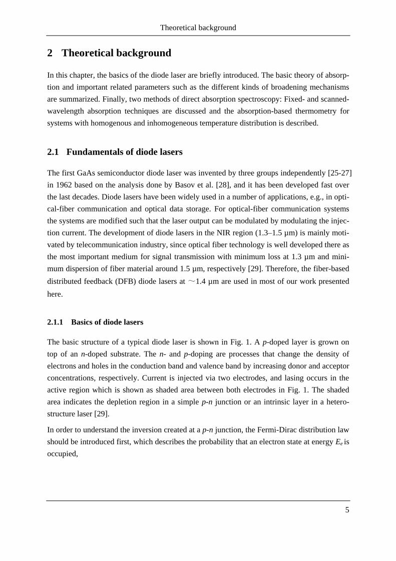
The basic structure of a typical diode laser is shown in Fig. 1. A p-doped layer is grown on
top of an n-doped substrate. The n- and p-doping are processes that change the density of
electrons and holes in the conduction band and valence band by increasing donor and acceptor
concentrations, respectively. Current is injected via two electrodes, and lasing occurs in the
active region which is shown as shaded area between both electrodes in Fig. 1. The shaded
area indicates the depletion region in a simple p-n junction or an intrinsic layer in a hetero-
structure laser [29].
In order to understand the inversion created at a p-n junction, the Fermi-Dirac distribution law
should be introduced first, which describes the probability that an electron state at energy Ee is
occupied,
Theoretical background
6
(1)
where EF is the Fermi energy, which is the chemical potential of electrons in semiconductors,
k is the Boltzmann constant and T is the temperature. At T = 0 K, according to eq. 1, all the
states below EF are filled with electrons, and those above it are empty. Due to the current flow
in the p-n junction, a number of electrons and holes are created by the applied potential, the
quasi-Fermi levels EFc and EFv are used for the conduction band and valence band, respective-
ly.
Fig. 1: Schematic drawing of a diode laser [29]
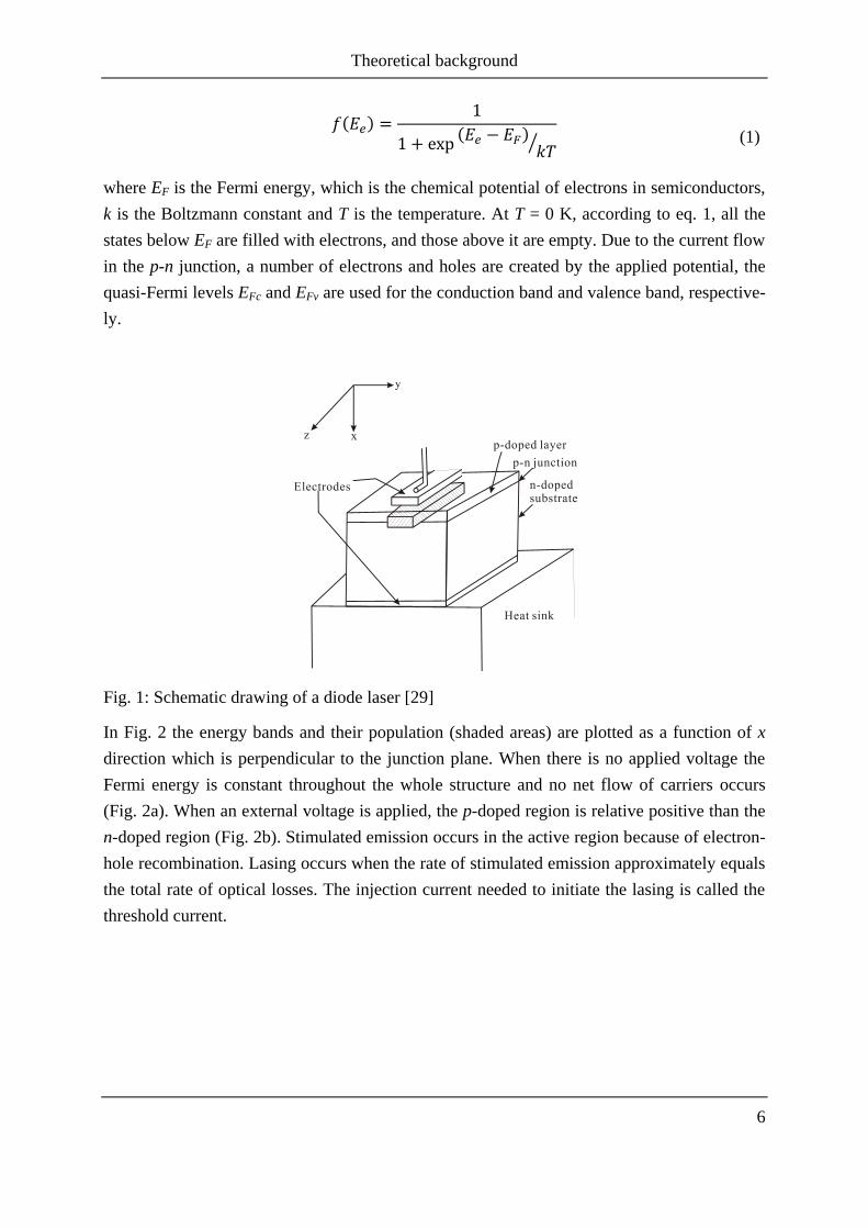
In Fig. 2 the energy bands and their population (shaded areas) are plotted as a function of x
direction which is perpendicular to the junction plane. When there is no applied voltage the
Fermi energy is constant throughout the whole structure and no net flow of carriers occurs
(Fig. 2a). When an external voltage is applied, the p-doped region is relative positive than the
n-doped region (Fig. 2b). Stimulated emission occurs in the active region because of electron-
hole recombination. Lasing occurs when the rate of stimulated emission approximately equals
the total rate of optical losses. The injection current needed to initiate the lasing is called the
threshold current.
Theoretical background
7
(a) (b)
Fig. 2: Electron energy and occupation perpendicular to the p-n junction (a) without an ap-
plied voltage and (b) with a forward biased applied voltage [29]
Several types of diode lasers have been developed in the last decades, e.g., edge-emitting las-
ers: Fabry-Perot (FP) laser; distributed Bragg grating (DBR) and distributed feedback (DFB)
lasers, and surface-emitting laser: Vertical cavity surface emitting lasers (VCSELs), quantum
cascade lasers and external cavity lasers. However, only the edge-emitting lasers will be dis-
cussed further in this thesis. The structure of these lasers is such that the emitted laser beams
and laser cavities are parallel to the laser substrates.
2.1.2 Fabry-Perot laser
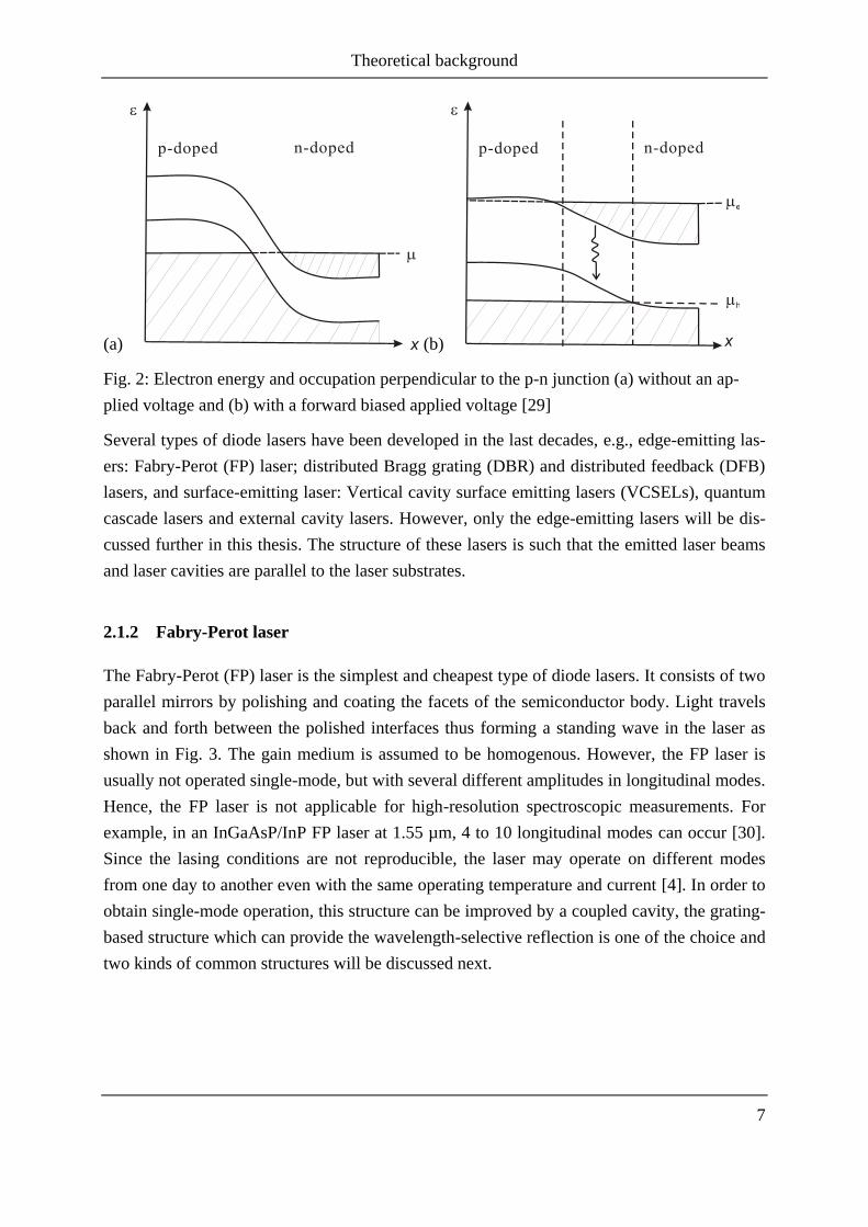
The Fabry-Perot (FP) laser is the simplest and cheapest type of diode lasers. It consists of two
parallel mirrors by polishing and coating the facets of the semiconductor body. Light travels
back and forth between the polished interfaces thus forming a standing wave in the laser as
shown in Fig. 3. The gain medium is assumed to be homogenous. However, the FP laser is
usually not operated single-mode, but with several different amplitudes in longitudinal modes.
Hence, the FP laser is not applicable for high-resolution spectroscopic measurements. For
example, in an InGaAsP/InP FP laser at 1.55 µm, 4 to 10 longitudinal modes can occur [30].
Since the lasing conditions are not reproducible, the laser may operate on different modes
from one day to another even with the same operating temperature and current [4]. In order to
obtain single-mode operation, this structure can be improved by a coupled cavity, the grating-
based structure which can provide the wavelength-selective reflection is one of the choice and
two kinds of common structures will be discussed next.
Theoretical background
8
Fig. 3: Schematic drawing of FP laser in the longitudinal axis
2.1.3 DBR and DFB diode lasers
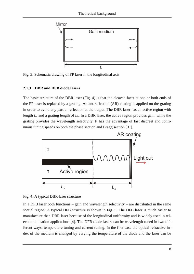
The basic structure of the DBR laser (Fig. 4) is that the cleaved facet at one or both ends of
the FP laser is replaced by a grating. An antireflection (AR) coating is applied on the grating
in order to avoid any partial reflection at the output. The DBR laser has an active region with
length La and a grating length of Lb. In a DBR laser, the active region provides gain, while the
grating provides the wavelength selectivity. It has the advantage of fast discreet and conti-
nuous tuning speeds on both the phase section and Bragg section [31].
Fig. 4: A typical DBR laser structure
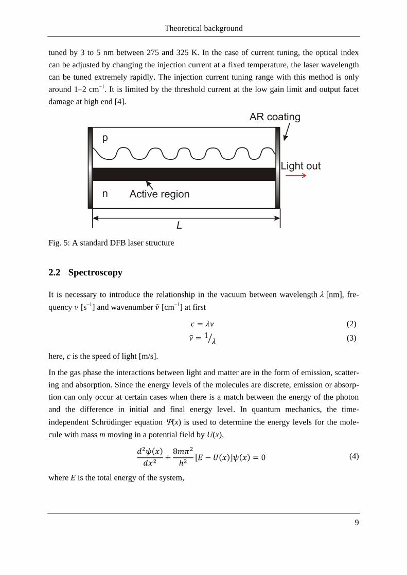
In a DFB laser both functions – gain and wavelength selectivity – are distributed in the same
spatial region: A typical DFB structure is shown in Fig. 5. The DFB laser is much easier to
manufacture than DBR laser because of the longitudinal uniformity and is widely used in tel-
ecommunication applications [4]. The DFB diode lasers can be wavelength-tuned in two dif-
ferent ways: temperature tuning and current tuning. In the first case the optical refractive in-
dex of the medium is changed by varying the temperature of the diode and the laser can be
Theoretical background
9
tuned by 3 to 5 nm between 275 and 325 K. In the case of current tuning, the optical index
can be adjusted by changing the injection current at a fixed temperature, the laser wavelength
can be tuned extremely rapidly. The injection current tuning range with this method is only
around 1–2 cm–1
. It is limited by the threshold current at the low gain limit and output facet
damage at high end [4].
Fig. 5: A standard DFB laser structure
2.2 Spectroscopy
It is necessary to introduce the relationship in the vacuum between wavelength[nm], fre-
quency [s–1
] and wavenumber [cm–1
] at first
(2)
(3)
here, c is the speed of light [m/s].
In the gas phase the interactions between light and matter are in the form of emission, scatter-
ing and absorption. Since the energy levels of the molecules are discrete, emission or absorp-
tion can only occur at certain cases when there is a match between the energy of the photon
and the difference in initial and final energy level. In quantum mechanics, the time-
independent Schrödinger equation (x) is used to determine the energy levels for the mole-
cule with mass m moving in a potential field by U(x),
(4)
where E is the total energy of the system,

Theoretical background
10
(5)
where h is Planck„s constant. Eelec is the electronic energy, Evib is the vibrational energy and
Erot is the rotational energy. They are depending on quantum numbers.
If one assumes the diatomic molecule is a rigid rotor the rotational energy can be obtained as
(6)
where J = 0, 1, 2, 3, … is the rotational quantum number and B [cm–1
] is the rotational con-
stant. For pure rotational lines (absorption or emission), the change in rotational quantum
number is J = ±1. And the rotational frequencies for these transitions are given by
(7)
where J’ and J” are the quantum numbers for the upper and lower state, respectively.
If one further assumes that the diatomic molecule is a simple harmonic oscillator (SHO), the
vibrational energy is given by
(8)
where = 0, 1, 2, 3,… is the vibrational quantum number, and we is the energy spacing be-
tween adjacent quantum states. The quantum mechanics solution for absorption and emission
assumed by the SHO model leads to a simple selection rule that says that the change in vibra-
tional quantum number is = ± 1.
2.2.1 Boltzmann distribution
The Boltzmann equation describes the temperature-dependent population distribution of the
molecules in their allowed quantum states. The fraction of molecules or atoms in energy level
i can be described by [32],
(9)
where gi is the degeneracy of level i, i is the common energy for state i, N is the total number
of molecules,
(10)
and the partition function Q is given by,
Theoretical background
11
(11)
which in this approximation can also be described as the product for rotational, vibrational
and electronic partition functions ,that are Qrot, Qvib, and Qelec, respectively.
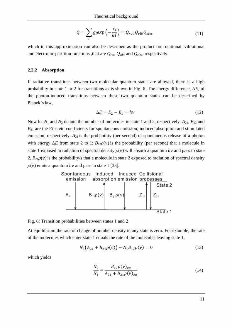
2.2.2 Absorption
If radiative transitions between two molecular quantum states are allowed, there is a high
probability in state 1 or 2 for transitions as is shown in Fig. 6. The energy difference, ΔE, of
the photon-induced transitions between these two quantum states can be described by
Planck‟s law,
(12)
Now let N1 and N2 denote the number of molecules in state 1 and 2, respectively. A21, B12 and
B21 are the Einstein coefficients for spontaneous emission, induced absorption and stimulated
emission, respectively. A21 is the probability (per second) of spontaneous release of a photon
with energy ΔE from state 2 to 1; B12( ) is the probability (per second) that a molecule in
state 1 exposed to radiation of spectral density ( ) will absorb a quantum h and pass to state
2, B21( ) is the probability/s that a molecule in state 2 exposed to radiation of spectral density
( ) emits a quantum h and pass to state 1 [33].
Fig. 6: Transition probabilities between states 1 and 2
At equilibrium the rate of change of number density in any state is zero. For example, the rate
of the molecules which enter state 1 equals the rate of the molecules leaving state 1,
(13)
which yields
(14)
Theoretical background
12
On the other hand, the ratio of the number density between the two quantum states can also be
expressed with the Boltzmann fraction
(15)
Compare eq. 14 with eq. 15,(v)eq will be obtained as
(16)
It follows that
(17)
(18)
When light enters a gas medium with differential length dx, the spectral absorbance v is de-
fined as the fraction of the incident light Iv over the frequency range [ , + ] that is ab-
sorbed; it can be also described as the product of absorption coefficient kv and length dx [33].
the absorption coefficient can be expressed as
(20)
The change in intensity after transmitting the gas medium (dIv) is the net combination of
the effects of absorption and emission [33]
(21)
where n1 and n2 are the number densities in states 1 and 2, respectively.
Hence,
(22)
therefore, kv can be described as
(23)
The normalized line shape function is defined as
Theoretical background
13
(24)
such that its integral over frequency is unity,
(25)
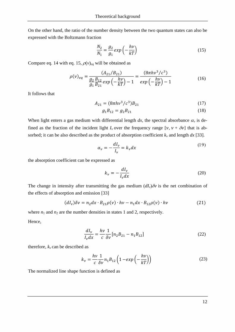
Fig. 7: The lineshape function for a transition located at 0
A typical lineshape of an isolated line centered at 0 is shown in Fig. 7. The lineshape func-
tion has a maximum value ( ) at the line center, and the width of the line can be described
by the full width at half maximum (FWHM) ∆ .
For the frequency range [ , + ], multiply ( ) from eq. 13 to eq. 22 and kv can be ex-
pressed as when considering the line shape function [33]
(26)
Integrating kv over the frequency range yields the line strength S12
(27)
(28)

Theoretical background
14
2.2.3 Beer-Lambert law
The typical setup of an absorption-spectroscopy experiment is sketched in Fig. 8. The laser is
used as a radiation source, which sends a beam with the initial intensity I0 through a gas me-
dium with a path length L, and the transmitted light intensity It behind the gas medium can be
recorded by a detector.
Fig. 8: Schematic of absorption-spectroscopy experimental setup
The basic law of absorption spectroscopy is the Beer-Lambert law
(29)
where is the transmission, kv [cm–1
] is the spectral absorption coefficient, n is the number
density of the absorbing species [molecules/cm3] and v [cm
2/molecules] is the frequency-
dependent absorption cross-section. For an isolated transition i,
(30)
where p [bar] is the total pressure of the gas medium, xabs is the mole fraction of the absorp-
tion species of interest, ( ) is the lineshape function, Si(T) [cm–2
bar–1
] is the line strength of
the transition at temperature T [K], which is only a function of T,
(31)
k is Boltzmann‟s constant, v0 is the center frequency of the transition, S(T0) denotes the line
strength at a reference temperature T0 (296 K), Q is the partition function and E” is the lower-
state energy of the quantum transition. These parameters at reference temperature can be
measured in a reference cell or obtained from the HITRAN database [16-17]. The last ratio of
eq. 31 can be neglected in a small temperature and frequency range.

Theoretical background
15
The partition function of water vapor can be described over a range of temperatures by a
third-order polynomial fit to a calculated partition function summation, the coefficients of the
polynomial expression aQ, bQ, cQ, and dQ are listed in Table 1 [16].
(32)
Table 1: Coefficients of the polynomial expression for the partition function of water vapor
[16]
Coefficients 70 K < T < 405 K 400 K < T < 1500 K 1500 K < T < 3005 K
aQ –0.44405 × 101 -0.94327 × 10² –0.11727 × 10⁴
bQ 0.27678 × 100 0.81903 × 100 0.29261 × 101
cQ 0.12536 × 10⁻² 0.74005 × 10⁻⁴ –0.13299 × 10⁻²
dQ –0.48938 × 10⁻⁶ 0.42437 × 10⁻⁶ 0.74356 × 10⁻⁶
Usually, the absorbance v can be described as
(33)
The integrated area Ai under the lineshape can be calculated as the integral of the absorbance,
(34)
which is only related to the partial pressure pxabs, pathlength and the temperature depended
line strength.
2.3 Line broadening mechanisms
The absorption lineshape broadening occurs when the absorbing molecules interact with light
or the energy levels of the transition are perturbed by physical mechanisms [34-35]. The
broadening mechanisms can be classified into two groups: homogenous broadening and in-
homogeneous broadening. The homogenous broadening mechanisms affect all the molecules
the same way. However, in the inhomogeneous broadening mechanisms, there are separate
classes or subgroups for which the interaction varies. The most important broadening mechan-
isms are discussed below [33].
Theoretical background
16
The Heisenberg uncertainty principle describes the relationship between the uncertainties of
these energy levels with their lifetimes, the uncertainty in the energy level i is limited by
(35)
where i is the lifetime of level i. The total uncertainty of a transition in units of frequency ∆v
can be given by
(36)
where „ and „„ are the lifetimes for the upper and lower states. Since the uncertainty is ho-
mogenous for all the molecules, the broadening is homogenous. The resulting lineshape func-
tion (v) can be derived as a form of Lorentzian function [36]:
(37)
where v0 is the line center. There are several different mechanisms which lead to line broaden-
ing. Three main types of broadening are described below.
2.3.1 Collisional broadening and shift
Collisional broadening is the other most important homogenous broadening mechanism. The
lifetime of an energy state can be shortened because of perturbations that occur during colli-
sions. According to eq. 36, the reduced lifetime leads to a broader linewidth. And it also can
be expressed by a Lorentzian profile [36]:
(38)
where ΔvC is the collisional FWHM and ΔvS is the pressure-induced frequency shift. If colli-
sions occur between identical species this is called self-broadening, while when it takes place
between different species it is called foreign broadening and needs to be known for each spe-
cies i. Both ΔvC and ΔvS are proportional to pressure p
(39)
(40)
Theoretical background
17
where xi is the mole fraction of the component i, and i and i are the collisional line broaden-
ing half-width and shifting coefficients due to the perturbation by the ith
component. The
broadening coefficient i is a function of temperature according to the following expression:
(41)
(42)
where T0 is the reference temperature, ni and mi are the corresponding temperature-dependent
coefficients which generally are determined experimentally.
2.3.2 Doppler broadening
Doppler broadening is the dominant inhomogeneous broadening mechanism. If the direction
of a molecule‟s (with mass m) velocity component is consistent with the light‟s propagation
path, there will be a frequency shift called Doppler shift. The values of velocities of molecules
are described by the Maxwellian velocity distribution function. Each group of molecules with
velocities in a small interval is considered part of a specific velocity class. The Maxwellian
velocity distribution function describes the fraction of molecules in each class. The distribu-
tion function leads to a Doppler lineshape function D with a Gaussian form:
(43)
the Gaussian lineshape at line center v0 is
(44)
where ΔvD is the Doppler half width (FWHM) given by
(45)
which also can be expressed as
(46)
where v0 [cm–1
] is the wavenumber of the line center, T [K] is the temperature, and M
[g/mole] is the molecular mass. When temperature increases the Doppler half width will be
bigger, and hence, the line is broadened. Thus, the Doppler half width can be used to roughly
Theoretical background
18
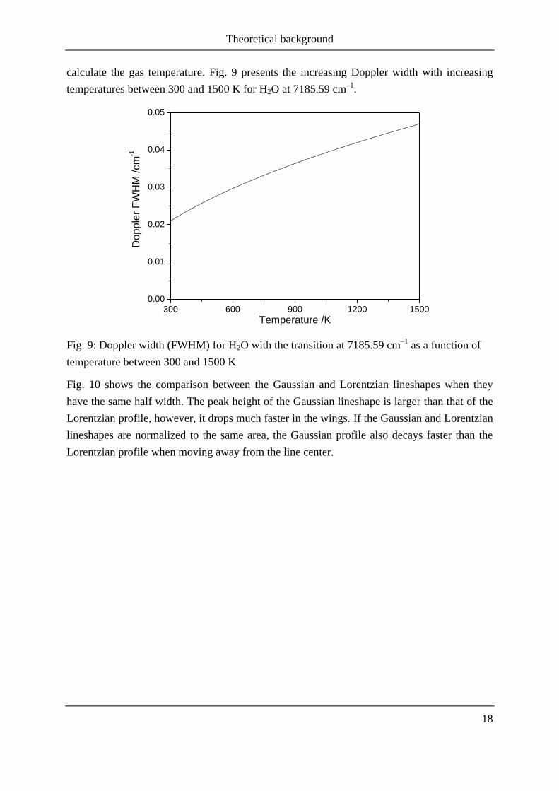
calculate the gas temperature. Fig. 9 presents the increasing Doppler width with increasing
temperatures between 300 and 1500 K for H2O at 7185.59 cm–1
.
300 600 900 1200 1500
0.00
0.01
0.02
0.03
0.04
0.05
Dopple
r F
WH
M /
cm
-1
Temperature /K
Fig. 9: Doppler width (FWHM) for H2O with the transition at 7185.59 cm–1
as a function of
temperature between 300 and 1500 K
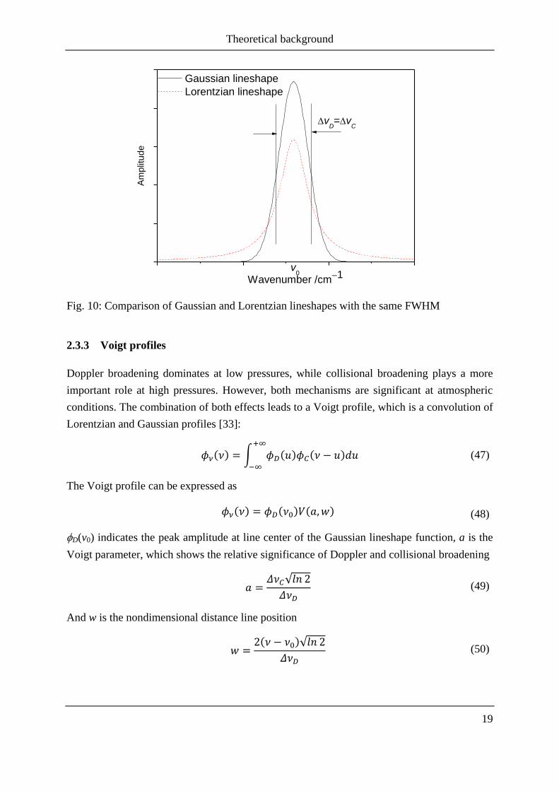
Fig. 10 shows the comparison between the Gaussian and Lorentzian lineshapes when they
have the same half width. The peak height of the Gaussian lineshape is larger than that of the
Lorentzian profile, however, it drops much faster in the wings. If the Gaussian and Lorentzian
lineshapes are normalized to the same area, the Gaussian profile also decays faster than the
Lorentzian profile when moving away from the line center.
Theoretical background
19
Wavenumber /cm1
Am
plit
ud
e
v0
Gaussian lineshape
Lorentzian lineshape
vD=v
C
Fig. 10: Comparison of Gaussian and Lorentzian lineshapes with the same FWHM
2.3.3 Voigt profiles
Doppler broadening dominates at low pressures, while collisional broadening plays a more
important role at high pressures. However, both mechanisms are significant at atmospheric
conditions. The combination of both effects leads to a Voigt profile, which is a convolution of
Lorentzian and Gaussian profiles [33]:
(47)
The Voigt profile can be expressed as
(48)
D(v0) indicates the peak amplitude at line center of the Gaussian lineshape function, a is the
Voigt parameter, which shows the relative significance of Doppler and collisional broadening
(49)
And w is the nondimensional distance line position
(50)

Theoretical background
20
The Voigt function V(a,w) can be determined by mathematical routines. A number of numeri-
cal approximations for the Voigt lineshape has been published before [37-38], one of the most
common used assumption is the algorithm published by Humlicek et al. [39].
2.4 Direct absorption spectroscopy
There are typically two kinds of experimental methods for direct absorption spectroscopy:
Fixed- and scanned- wavelength spectroscopy. Both of them have been widely used to meas-
ure a number of gas dynamic parameters, e.g. temperature, pressure, species concentration
and flow velocity [4].
2.4.1 Fixed-wavelength absorption spectroscopy
In fixed-wavelength absorption spectroscopy, the laser wavelength is fixed at the center of an
absorption line, or – if a broadband absorber is investigated – at a suitable position depending
on other measurement issues. The laser beam is sent through the gas medium and the trans-
mission is measured for a certain time period depending on the intended temporal resolution
of data acquisition. The method is easy to design and it can also achieve high sensor band-
width of several MHz in which allows the acquisition of highly transient events such as in IC
engines [40]. The wavelength selection range of this technique is relative large by tuning the
laser temperature while the laser current is constant. However, two aspects must be consi-
dered for this technique: one is non-resonant attenuation by unknown species or other effects
(scattering, extinction, dirty optics, beam steering), and the missing lineshape information. In
most practical environments, beam steering, window fouling and absorption by other liquid-
phase species will cause non-resonant attenuation of the laser beam. Hence, an additional non-
resonant laser must be combined to infer the non-absorbing baseline [40]. For the second as-
pect, as described above the lineshape of the absorption line depends on pressure, temperature
and absorber concentration. These parameters and their effects on the lineshape need to be
known beforehand for extracting meaningful quantitative information, i.e. concentration, from
the measurement.
2.4.2 Scanned-wavelength absorption spectroscopy
The scanned-wavelength absorption spectroscopy will compensate the drawbacks of the
fixed-wavelength absorption method [19, 41], and the schematic drawing of a typical
scanned-wavelength absorption setup is shown in Fig. 11. The laser wavelength is rapidly

Theoretical background
21
current-tuned by a saw-tooth signal generated by a function generator. The laser output is se-
parated into two parts by a splitter. The main portion of the beam is transmitted directly
through the gas medium onto a detector. A typical measured signal as a function of time is
shown in Fig. 12. A third-order polynomial is fitted to the baseline region of the signal as
shown by the dotted line in Fig. 12, while the absorption spectrum (here as a function of scan
time of the laser wavelength) will be obtained by subtracting the baseline. A fraction of the
incident beam is sent through a Fabry-Perot interferometer (etalon), and the transmission is
measured by a second detector.
Fig. 11: Schematic drawing of a typical scanned-wavelength absorption experiment
0 2 4 6 8 10
0.0
0.4
0.8
1.2
Time /ms
Sig
nal /V
Transmission signal
Regions used to
fit baseline
Baseline
Fig. 12: Detected signal for a direct absorption scan near 1353 nm
Theoretical background
22
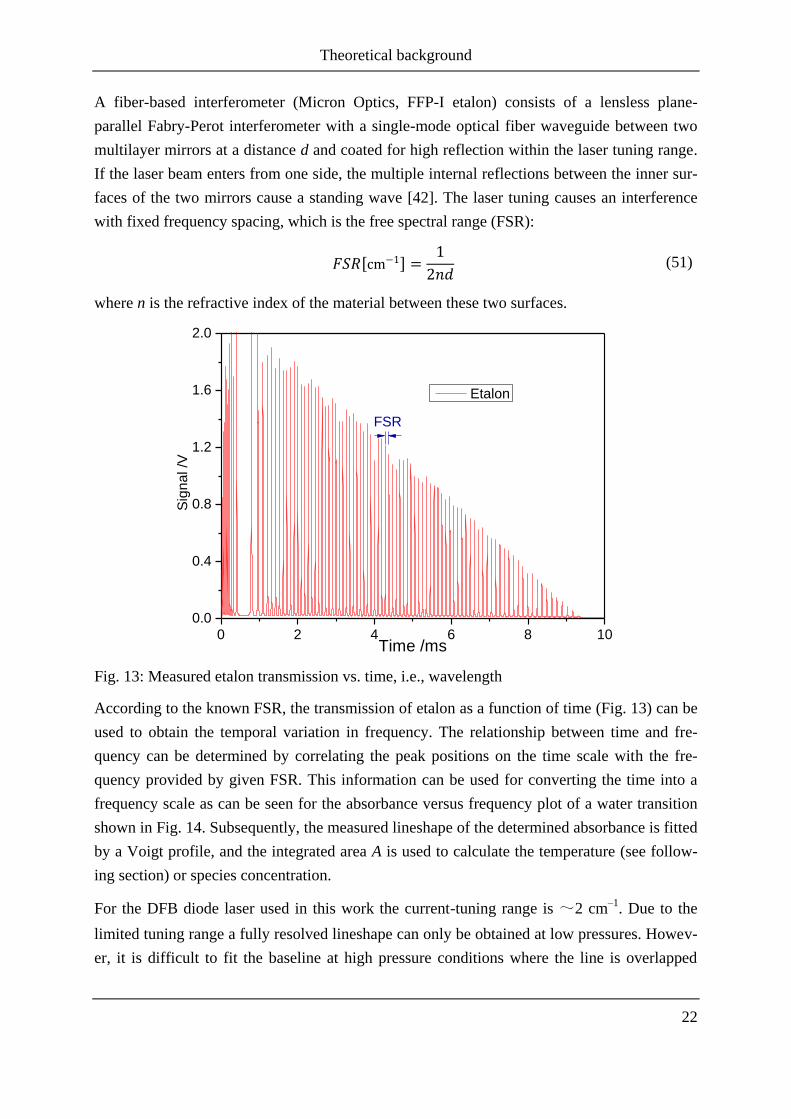
A fiber-based interferometer (Micron Optics, FFP-I etalon) consists of a lensless plane-
parallel Fabry-Perot interferometer with a single-mode optical fiber waveguide between two
multilayer mirrors at a distance d and coated for high reflection within the laser tuning range.
If the laser beam enters from one side, the multiple internal reflections between the inner sur-
faces of the two mirrors cause a standing wave [42]. The laser tuning causes an interference
with fixed frequency spacing, which is the free spectral range (FSR):
(51)
where n is the refractive index of the material between these two surfaces.
0 2 4 6 8 10
0.0
0.4
0.8
1.2
1.6
2.0
Sig
na
l /V
Time /ms
Etalon
FSR
Fig. 13: Measured etalon transmission vs. time, i.e., wavelength
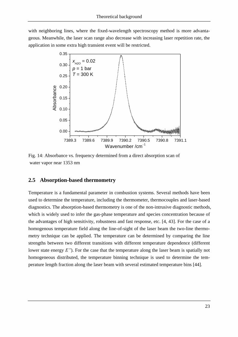
According to the known FSR, the transmission of etalon as a function of time (Fig. 13) can be
used to obtain the temporal variation in frequency. The relationship between time and fre-
quency can be determined by correlating the peak positions on the time scale with the fre-
quency provided by given FSR. This information can be used for converting the time into a
frequency scale as can be seen for the absorbance versus frequency plot of a water transition
shown in Fig. 14. Subsequently, the measured lineshape of the determined absorbance is fitted
by a Voigt profile, and the integrated area A is used to calculate the temperature (see follow-
ing section) or species concentration.
For the DFB diode laser used in this work the current-tuning range is ~2 cm–1
. Due to the
limited tuning range a fully resolved lineshape can only be obtained at low pressures. Howev-
er, it is difficult to fit the baseline at high pressure conditions where the line is overlapped
Theoretical background
23
with neighboring lines, where the fixed-wavelength spectroscopy method is more advanta-
geous. Meanwhile, the laser scan range also decrease with increasing laser repetition rate, the
application in some extra high transient event will be restricted.
7389.3 7389.6 7389.9 7390.2 7390.5 7390.8 7391.1
0.00
0.05
0.10
0.15
0.20
0.25
0.30
0.35
Absorb
ance
Wavenumber /cm1
xH2O
= 0.02
p = 1 bar
T = 300 K
Fig. 14: Absorbance vs. frequency determined from a direct absorption scan of
water vapor near 1353 nm
2.5 Absorption-based thermometry
Temperature is a fundamental parameter in combustion systems. Several methods have been
used to determine the temperature, including the thermometer, thermocouples and laser-based
diagnostics. The absorption-based thermometry is one of the non-intrusive diagnostic methods,
which is widely used to infer the gas-phase temperature and species concentration because of
the advantages of high sensitivity, robustness and fast response, etc. [4, 43]. For the case of a
homogenous temperature field along the line-of-sight of the laser beam the two-line thermo-
metry technique can be applied. The temperature can be determined by comparing the line
strengths between two different transitions with different temperature dependence (different
lower state energy E”). For the case that the temperature along the laser beam is spatially not
homogeneous distributed, the temperature binning technique is used to determine the tem-
perature length fraction along the laser beam with several estimated temperature bins [44].
Theoretical background
24
2.5.1 System with homogenous temperature distribution
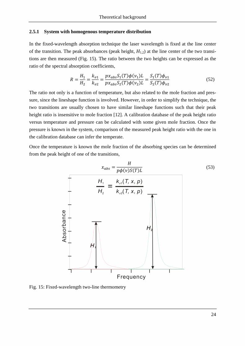
In the fixed-wavelength absorption technique the laser wavelength is fixed at the line center
of the transition. The peak absorbances (peak height, H1,2) at the line center of the two transi-
tions are then measured (Fig. 15). The ratio between the two heights can be expressed as the
ratio of the spectral absorption coefficients,
(52)
The ratio not only is a function of temperature, but also related to the mole fraction and pres-
sure, since the lineshape function is involved. However, in order to simplify the technique, the
two transitions are usually chosen to have similar lineshape functions such that their peak
height ratio is insensitive to mole fraction [12]. A calibration database of the peak height ratio
versus temperature and pressure can be calculated with some given mole fraction. Once the
pressure is known in the system, comparison of the measured peak height ratio with the one in
the calibration database can infer the temperate.
Once the temperature is known the mole fraction of the absorbing species can be determined
from the peak height of one of the transitions,
(53)
Fig. 15: Fixed-wavelength two-line thermometry
Theoretical background
25
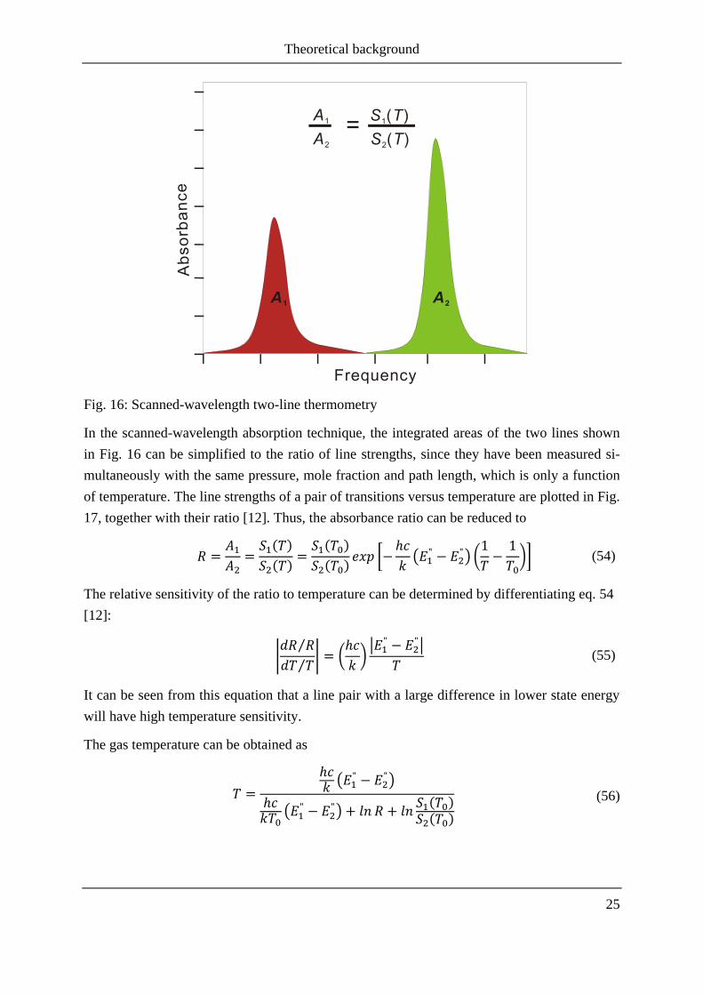
Fig. 16: Scanned-wavelength two-line thermometry
In the scanned-wavelength absorption technique, the integrated areas of the two lines shown
in Fig. 16 can be simplified to the ratio of line strengths, since they have been measured si-
multaneously with the same pressure, mole fraction and path length, which is only a function
of temperature. The line strengths of a pair of transitions versus temperature are plotted in Fig.
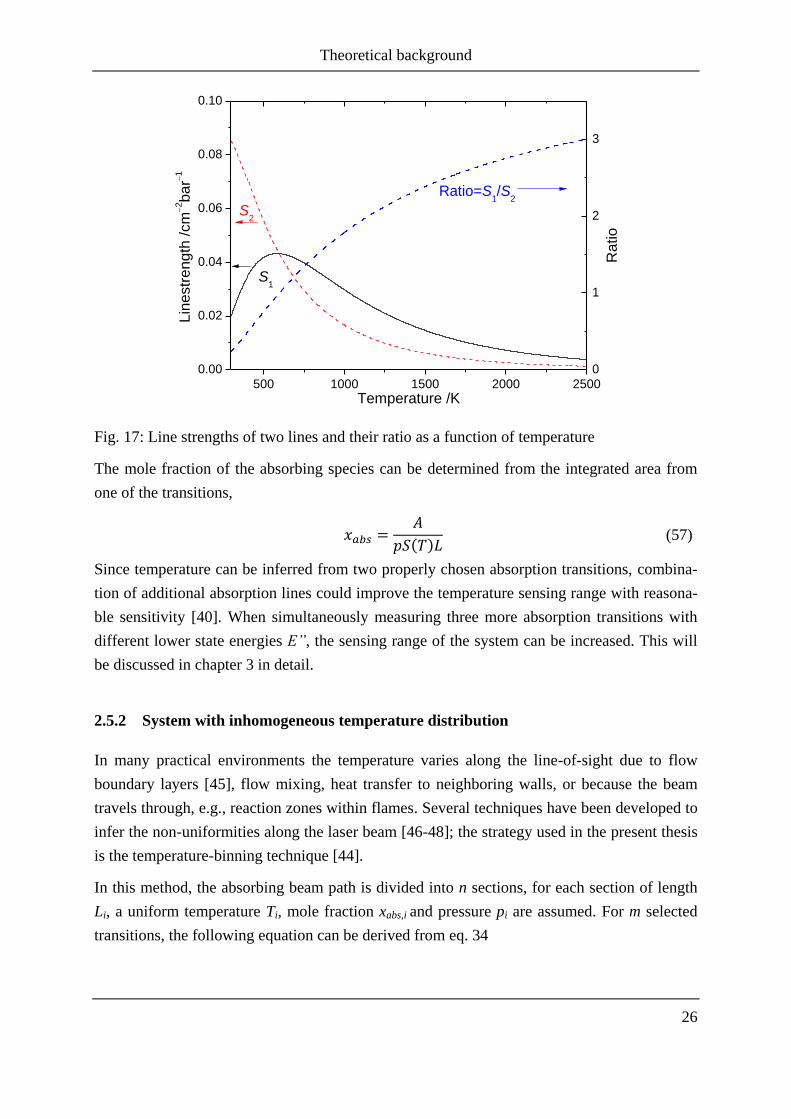
17, together with their ratio [12]. Thus, the absorbance ratio can be reduced to
(54)
The relative sensitivity of the ratio to temperature can be determined by differentiating eq. 54
[12]:
(55)
It can be seen from this equation that a line pair with a large difference in lower state energy
will have high temperature sensitivity.
The gas temperature can be obtained as
(56)
Theoretical background
26
500 1000 1500 2000 2500
0.00
0.02
0.04
0.06
0.08
0.10
Lin
estr
ength
/cm
2bar
1
Temperature /K
0
1
2
3
S1
S2
Ratio
Ratio=S1/S
2
Fig. 17: Line strengths of two lines and their ratio as a function of temperature
The mole fraction of the absorbing species can be determined from the integrated area from
one of the transitions,
(57)
Since temperature can be inferred from two properly chosen absorption transitions, combina-
tion of additional absorption lines could improve the temperature sensing range with reasona-
ble sensitivity [40]. When simultaneously measuring three more absorption transitions with
different lower state energies E”, the sensing range of the system can be increased. This will
be discussed in chapter 3 in detail.
2.5.2 System with inhomogeneous temperature distribution
In many practical environments the temperature varies along the line-of-sight due to flow
boundary layers [45], flow mixing, heat transfer to neighboring walls, or because the beam
travels through, e.g., reaction zones within flames. Several techniques have been developed to
infer the non-uniformities along the laser beam [46-48]; the strategy used in the present thesis
is the temperature-binning technique [44].
In this method, the absorbing beam path is divided into n sections, for each section of length
Li, a uniform temperature Ti, mole fraction xabs,i and pressure pi are assumed. For m selected
transitions, the following equation can be derived from eq. 34
Theoretical background
27
(58)
If the individual temperatures (T1, T2, … Tn) along the beam path are estimated, the line
strength matrix, which only is a function of temperature, can be calculated. The vector of ab-
sorbances Ai is the measured quantity. If the number of the selected absorption transitions m is
larger than the number of temperature bins n, the equation can be solved unambiguously by a
non-negative constrained least-square algorithm, which minimizes the following expression
[44].
(59)
with
(60)
When the pressure and mole fraction are assumed uniform along the beam path, the length
fraction fj for each temperature bin can be calculated,
(61)

Theoretical background
28
Sensor design
29
3 Sensor design
A suitable sensor design is the first step in absorption-based thermometry. This chapter first
discusses the basic structure and fundamental vibrational modes of water and an overview of
known water-vapor absorption lines in the HITRAN ([16]) spectroscopic database. The car-
bon dioxide absorption spectrum is also described. Then optimal line pair selection rules are
presented, and the multiplexing techniques for multi-line two-line thermometry are also de-
scribed. Finally, the 1.4 µm sensor used in the present work and the 2.7 µm laser applied in
future work are introduced.
3.1 Water vapor
Water (H2O) is one of the most important molecules in life. It is presented in three different
states of aggregation on earth: liquid (e.g., seawater), solid (e.g., ice) and gas (e.g., water va-
por). The water molecule has one oxygen and two hydrogen atoms connected by covalent
bonds.
Water vapor is the main product in hydrocarbon combustion, and mainly shows strong ab-
sorptions in the infrared region. Thus many spectroscopic sensors developed before [49-51],
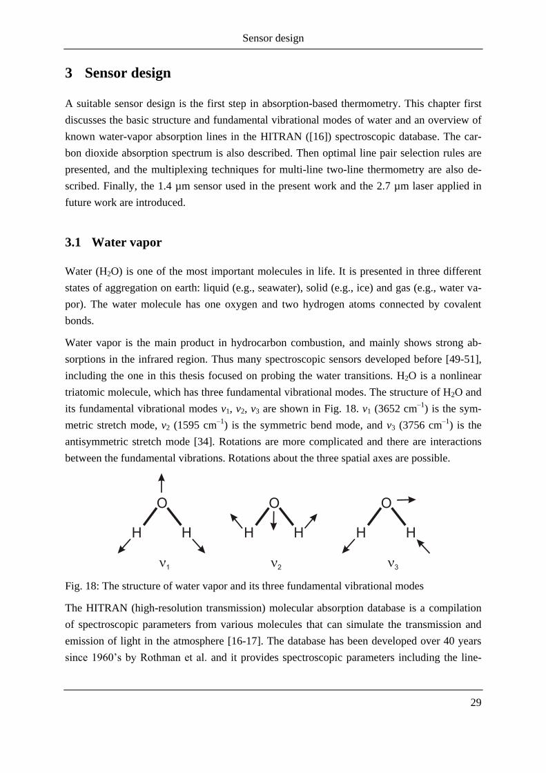
including the one in this thesis focused on probing the water transitions. H2O is a nonlinear
triatomic molecule, which has three fundamental vibrational modes. The structure of H2O and
its fundamental vibrational modes v1, v2, v3 are shown in Fig. 18. v1 (3652 cm–1
) is the sym-
metric stretch mode, v2 (1595 cm–1
) is the symmetric bend mode, and v3 (3756 cm–1
) is the
antisymmetric stretch mode [34]. Rotations are more complicated and there are interactions
between the fundamental vibrations. Rotations about the three spatial axes are possible.
Fig. 18: The structure of water vapor and its three fundamental vibrational modes
The HITRAN (high-resolution transmission) molecular absorption database is a compilation
of spectroscopic parameters from various molecules that can simulate the transmission and
emission of light in the atmosphere [16-17]. The database has been developed over 40 years
since 1960‟s by Rothman et al. and it provides spectroscopic parameters including the line-

Sensor design
30
center frequency v0 [cm–1
], lines strength S [cm–2
/bar], lower state energy E” [cm–1
], air-
broadening half-width air [cm–1
bar–1
], temperature-dependent exponents nair [–], self-
broadening coefficients self [cm–1
bar–1
] and air-induced frequency-shift coefficients air [cm–
1bar
–1]. There are more than 2.7 million spectral lines for 39 different molecules in the HI-
TRAN 2008 database [17]. However, the HITRAN database only contains data relevant to
atmospheric conditions where temperature ranges between 200 and 350 K. Hence, a high
temperature molecular database (HITEMP) was developed for improvement of data taken in
high temperature applications, e.g. combustion processes, exhaust plumes, etc. It is analogous
to HITRAN but encompasses many more bands and transitions than HITRAN [52]. There are
more than 114 million water lines in HITEMP 2010. The line-by-line data, including the im-
portant spectroscopic parameter can be manipulated by the JavaHAWKS (HITRAN atmos-
pheric workstation) software which is used to improve the cross-platform compatibility [53].
1.0 1.5 2.0 2.5 3.0 3.5 4.0
1E-4
1E-3
0.01
0.1
1
10
100
v1+v
2+v
3
v2+2v
3
2v1+v
2
v1+v
3
2v3
2v1
v2+v
3
v1+v
2
v3
v1
2v2
Lin
e s
trength
/cm
2/b
ar
Wavelength /µm
Room temperature
HITRAN 2004
Fig. 19: Absorption spectrum of water vapor at room temperature from 1 to 4 µm based on
HITRAN 2004 database
Since the water molecule has very small moment inertia, there are a large number of narrow-
band and closely spaced rovibrational absorption lines. In Fig. 19, the water vapor absorption
lines at room temperature from 1 to 4 µm based on the HITRAN database are plotted. The 2v1,
2v3 and v1+v3 absorption bands in the NIR region are popular for the sensor development
since fiber-based, single-mode tunable diode lasers are commercially available in that wave-
Sensor design
31
length range. Several researchers have chosen proper line pairs in this region to infer gas-
phase temperatures [54-55]. The selection strategies will be discussed in the next section. It is
also shown in Fig. 19 that in the region of the v1, v3 fundamental bands in the mid-infrared
(MIR) region, e.g. around 2.7 µm, the corresponding line strengths are 20 times larger than in
the NIR region. The transitions in this region are optimal to be used in the application with
low absorber concentration or short path lengths.
3.2 Carbon dioxide (CO2)
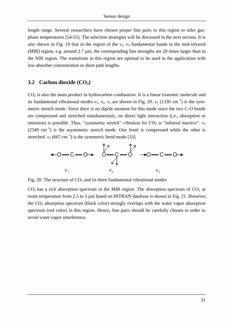
CO2 is also the main product in hydrocarbon combustion. It is a linear triatomic molecule and
its fundamental vibrational modes v1, v2, v3 are shown in Fig. 20. v1 (1330 cm–1
) is the sym-
metric stretch mode. Since there is no dipole moment for this mode since the two C-O bonds
are compressed and stretched simultaneously, no direct light interaction (i.e., absorption or
emission) is possible. Thus, “symmetric stretch” vibration for CO2 is “infrared inactive”. v3
(2349 cm–1
) is the asymmetric stretch mode. One bond is compressed while the other is
stretched. v2 (667 cm–1
) is the symmetric bend mode [33].
Fig. 20: The structure of CO2 and its three fundamental vibrational modes
CO2 has a rich absorption spectrum in the MIR region. The absorption spectrum of CO2 at
room temperature from 2.5 to 3 µm based on HITRAN database is shown in Fig. 21. However,
the CO2 absorption spectrum (black color) strongly overlaps with the water vapor absorption
spectrum (red color) in this region. Hence, line pairs should be carefully chosen in order to
avoid water vapor interference.

Sensor design
32
2.5 2.6 2.7 2.8 2.9 3.0
1E-5
1E-4
1E-3
0.01
0.1
1
10
100
Lin
estr
ength
/cm
2/b
ar
Wavelength /µm
Room temperature
HITRAN 2004
H2O
CO2
Fig. 21: Absorption spectrum of CO2 and H2O at room temperature from 2.5 to 3 µm based on
HITRAN 2004 database
3.3 Line selection strategies
Since the absorption sensor used in this thesis operates around 1.4 µm in the NIR region, this
section first focuses on describing the strategy of choosing proper line pairs between 1 and 2
µm for the conventional TDLAS two-line water vapor thermometry. The selection rules have
been introduced by the group of Prof. Hanson at Stanford University, USA, and are summa-
rized below [12,54]:
First, the selection of candidate H2O lines should be limited to the spectral region of 1.25–
1.65 µm, where H2O absorption spectra overlap with the most common telecommunication
bands, where optic fiber based diode lasers are widely available.
Second, both lines need sufficient absorption over the selected temperature range. A mini-
mum detectable absorbance (noise level, NL) of 10–4
and a desired signal/noise ratio (SNR) of
10 are given. It is required that the peak absorption must be greater than (NL) × (SNR), that is
10–3
. However, the product should be less than 0.8 to avoid “optically-thick” measurements.
Third, the two lines should have sufficiently different lower state energy to make sure that the
absorption ratio is sensitive to temperature. The larger the difference of the lower state energy
is, the better is the temperature sensitivity (see. eq. 55). However, there are still two limita-
tions. One is that lines with smaller E” have large absorbance at cold boundary layers. The
Sensor design
33
other is that lines with high E” always have very small absorbance, such that it is difficult to
obtain a reasonable signal-to-noise ratio (SNR) with the smaller E” lines when building the
ratio.
Fourth, both lines should be relatively free from interference of ambient H2O and cold boun-
dary layers. This can be achieved by using transitions with high ground-state energies. The
two lines should also be free of significant interference from nearby transitions.
A single laser covering the wavelength range of two adjacent water lines with the above men-
tioned properties is optimal because of the simplicity of experimental setup. However, only
few adjacent transition pairs exist which have proper spectroscopic parameters to enable sen-
sitive temperature measurements. Zhou et al. has chosen a single laser at 1398 nm (denoted as
laser 1) which was chosen here in a previous work [56] to measure the temperature in a pre-
mixed atmospheric-pressure burner. The spectroscopic parameters of the two transitions are
shown in Table 2 [12].
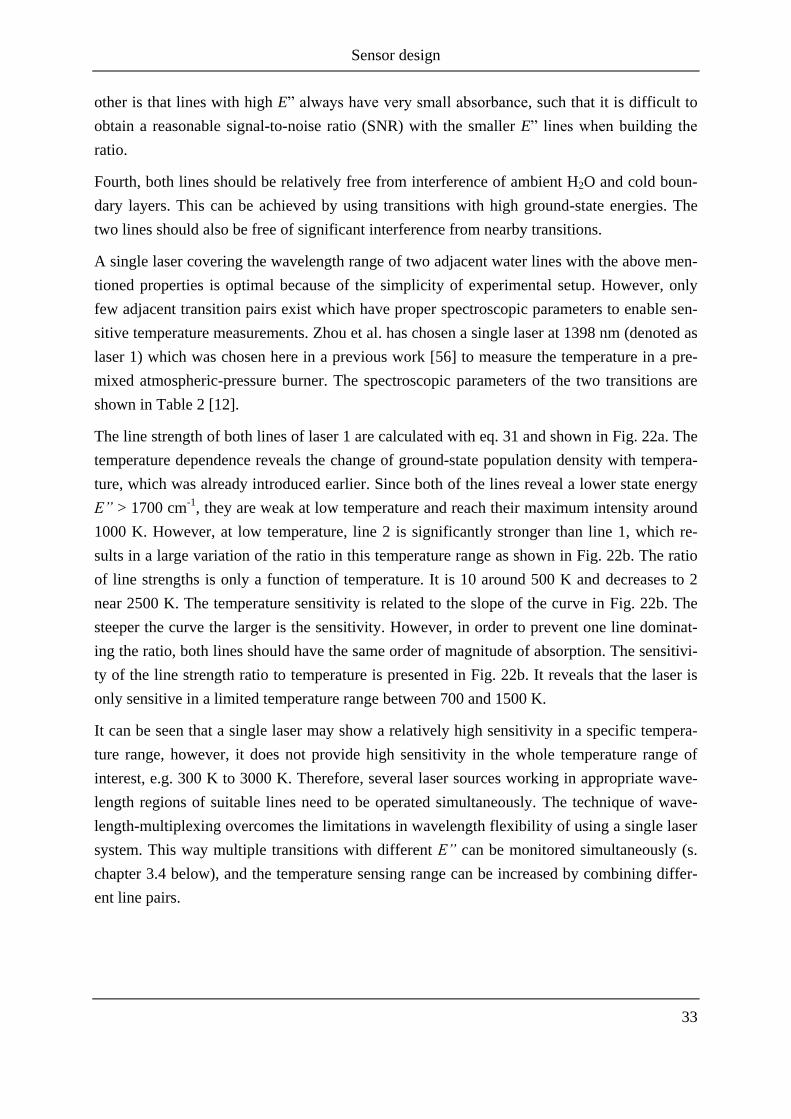
The line strength of both lines of laser 1 are calculated with eq. 31 and shown in Fig. 22a. The
temperature dependence reveals the change of ground-state population density with tempera-
ture, which was already introduced earlier. Since both of the lines reveal a lower state energy
E” > 1700 cm-1
, they are weak at low temperature and reach their maximum intensity around
1000 K. However, at low temperature, line 2 is significantly stronger than line 1, which re-
sults in a large variation of the ratio in this temperature range as shown in Fig. 22b. The ratio
of line strengths is only a function of temperature. It is 10 around 500 K and decreases to 2
near 2500 K. The temperature sensitivity is related to the slope of the curve in Fig. 22b. The
steeper the curve the larger is the sensitivity. However, in order to prevent one line dominat-
ing the ratio, both lines should have the same order of magnitude of absorption. The sensitivi-
ty of the line strength ratio to temperature is presented in Fig. 22b. It reveals that the laser is
only sensitive in a limited temperature range between 700 and 1500 K.
It can be seen that a single laser may show a relatively high sensitivity in a specific tempera-
ture range, however, it does not provide high sensitivity in the whole temperature range of
interest, e.g. 300 K to 3000 K. Therefore, several laser sources working in appropriate wave-
length regions of suitable lines need to be operated simultaneously. The technique of wave-
length-multiplexing overcomes the limitations in wavelength flexibility of using a single laser
system. This way multiple transitions with different E” can be monitored simultaneously (s.
chapter 3.4 below), and the temperature sensing range can be increased by combining differ-
ent line pairs.
Sensor design
34
500 1000 1500 2000 2500
0.000
0.002
0.004
0.006
0.008
0.010
a)
Lin
estr
en
gth
/cm
2bar
1
Temperature /K
Line 1
Line 2
500 1000 1500 2000 2500
0
1
2
3
4
Ra
tio
(dR
/R)/
(dT
/T)
Temperature /K
b)0
1
2
3
4
5
slope
slope
Fig. 22: Line strengths (a) and ratio (b) of line strength (blue dashed line) and its sensitivity
(green line) vs. temperature for the lines 1 and 2 of laser 1 described in Table 2
Mattison et al. have set up a multiplexed diode-laser temperature sensor for measuring in a
valveless pulse detonation engine [57]. At IVG such a system was used previously for tem-
perature measurements in a shock tube [58]. The spectroscopic parameters of the used transi-
tions are also listed in Table 2 (laser 1–4).
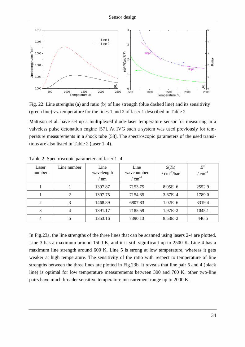
Table 2: Spectroscopic parameters of laser 1‒4
Laser
number Line number Line
wavelength
/ nm
Line
wavenumber
/ cm–1
S(T0)
/ cm–2/bar
E”
/ cm–1
1 1 1397.87 7153.75 8.05E–6 2552.9
1 2 1397.75 7154.35 3.67E–4 1789.0
2 3 1468.89 6807.83 1.02E–6 3319.4
3 4 1391.17 7185.59 1.97E–2 1045.1
4 5 1353.16 7390.13 8.53E–2 446.5
In Fig.23a, the line strengths of the three lines that can be scanned using lasers 2-4 are plotted.
Line 3 has a maximum around 1500 K, and it is still significant up to 2500 K. Line 4 has a
maximum line strength around 600 K. Line 5 is strong at low temperature, whereas it gets
weaker at high temperature. The sensitivity of the ratio with respect to temperature of line
strengths between the three lines are plotted in Fig.23b. It reveals that line pair 5 and 4 (black
line) is optimal for low temperature measurements between 300 and 700 K, other two-line
pairs have much broader sensitive temperature measurement range up to 2000 K.
Sensor design
35
500 1000 1500 2000 2500
0.00
0.02
0.04
0.06
0.08
0.10
a)
Lin
e s
tre
ng
th /
cm
2bar
1
Temperature /K
Line 3
Line 4
Line 5
500 1000 1500 2000 2500
0
2
4
6
8
10
(dR
/R)/
(dT
/T)
Temperature /K
Ratio sensitivity line 4/ line 3
Ratio sensitivity line 5/ line 3
Ratio sensitivity line 5/ line 4
b)
Fig. 23: Line strengths (a) and ratio sensitivity (b) vs. temperature for the lines 3–5 of
laser 2–4 described in Table 2
In the following these four laser sources covering five transitions will be applied in a low-
pressure reactor described in Chapter 4. Laser 3 and 4 will later further be applied for the liq-
uid film measurement and introduced in Chapter 5.
3.4 Multiplexing techniques
The advantage of the wavelength-multiplexing technique has been introduced in the last sec-
tion. Several lasers are combined together and transmitted along the same optical path. There
are three different kinds of techniques usually used for this method: Time-Division Multiplex-
ing (TDM), Frequency-Division Multiplexing (FDM) and Wavelength-Division Multiplexing
(WDM). In order to simplify the description, for all the methods introduced below examples
are restricted to two-line techniques. The FDM is typically used in modulation spectroscopy
where the different wavelengths are modulated at different frequencies which is not used in
the present thesis [59]. The other two methods are introduced in detail as below.
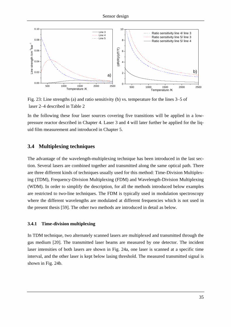
3.4.1 Time-division multiplexing
In TDM technique, two alternately scanned lasers are multiplexed and transmitted through the
gas medium [20]. The transmitted laser beams are measured by one detector. The incident
laser intensities of both lasers are shown in Fig. 24a, one laser is scanned at a specific time
interval, and the other laser is kept below lasing threshold. The measured transmitted signal is
shown in Fig. 24b.
Sensor design
36
Fig. 24: The incident (a) and transmitted (b) laser intensities of TDM
The advantage of this technique is the simplicity of the optical setup, since only one detector
is used. However, there are two drawbacks. One is that the laser intensities are not measured
simultaneously. Therefore, the technique can only be applied in temperature steady environ-
ments, which will lead to large measurement uncertainties for the applications in highly tran-
sient events. The other drawback is that the sensor bandwidth is limited, since each laser is
only scanned during a short time period. As will be discussed in Chapter 5, the TDM tech-
nique was used for water film thickness measurements in a flow channel.
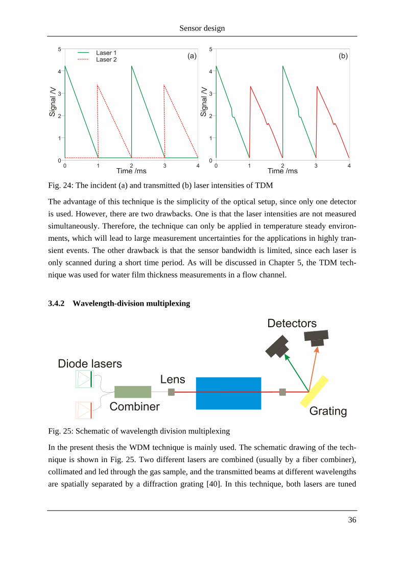
3.4.2 Wavelength-division multiplexing
Fig. 25: Schematic of wavelength division multiplexing
In the present thesis the WDM technique is mainly used. The schematic drawing of the tech-
nique is shown in Fig. 25. Two different lasers are combined (usually by a fiber combiner),
collimated and led through the gas sample, and the transmitted beams at different wavelengths
are spatially separated by a diffraction grating [40]. In this technique, both lasers are tuned

Sensor design
37
simultaneously by a continuous saw-tooth signal (shown in Fig. 26a). The transmitted intensi-
ties of each laser are detected by individual detectors and shown in Fig. 26b and Fig. 26c.
Fig. 26: The incident (a) and transmitted laser intensities of laser 1 (b) and laser 2 (c) of
WDM
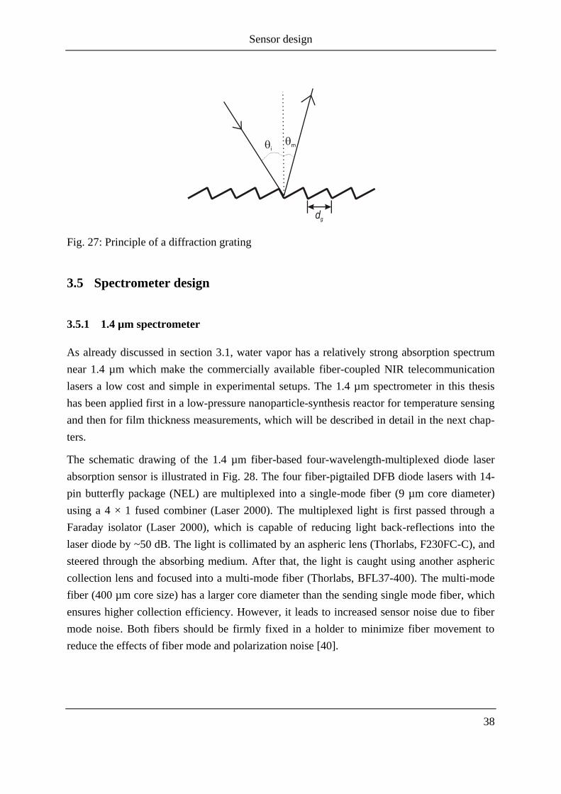
A diffraction grating is an optical component with parallel grooves with distance dg, as shown
in Fig. 27. The grating equation is given by
(62)
where i is the incident angle, m is the diffracted angle, m is the order of diffraction and is
the wavelength. The diffracted angle depends on wavelength. Thus, the multiple transmitted
laser beams of different wavelength after diffraction will propagate in different directions and
can be steered onto different detectors as shown in Fig. 25. It should be noticed that WDM
cannot be used for a large number of wavelengths due to the overlap between different order
reflections or the wavelength separation is geometrically insufficient.
Sensor design
38
Fig. 27: Principle of a diffraction grating
3.5 Spectrometer design
3.5.1 1.4 µm spectrometer
As already discussed in section 3.1, water vapor has a relatively strong absorption spectrum
near 1.4 µm which make the commercially available fiber-coupled NIR telecommunication
lasers a low cost and simple in experimental setups. The 1.4 µm spectrometer in this thesis
has been applied first in a low-pressure nanoparticle-synthesis reactor for temperature sensing
and then for film thickness measurements, which will be described in detail in the next chap-
ters.
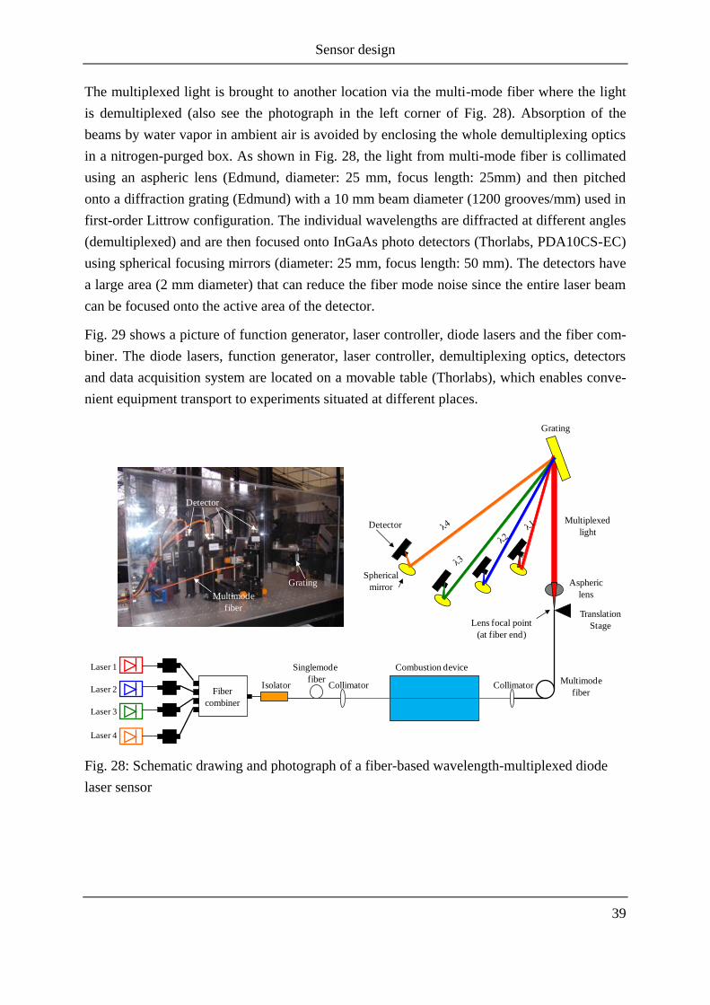
The schematic drawing of the 1.4 µm fiber-based four-wavelength-multiplexed diode laser
absorption sensor is illustrated in Fig. 28. The four fiber-pigtailed DFB diode lasers with 14-
pin butterfly package (NEL) are multiplexed into a single-mode fiber (9 µm core diameter)
using a 4 × 1 fused combiner (Laser 2000). The multiplexed light is first passed through a
Faraday isolator (Laser 2000), which is capable of reducing light back-reflections into the
laser diode by ~50 dB. The light is collimated by an aspheric lens (Thorlabs, F230FC-C), and
steered through the absorbing medium. After that, the light is caught using another aspheric
collection lens and focused into a multi-mode fiber (Thorlabs, BFL37-400). The multi-mode
fiber (400 µm core size) has a larger core diameter than the sending single mode fiber, which
ensures higher collection efficiency. However, it leads to increased sensor noise due to fiber
mode noise. Both fibers should be firmly fixed in a holder to minimize fiber movement to
reduce the effects of fiber mode and polarization noise [40].
Sensor design
39
The multiplexed light is brought to another location via the multi-mode fiber where the light
is demultiplexed (also see the photograph in the left corner of Fig. 28). Absorption of the
beams by water vapor in ambient air is avoided by enclosing the whole demultiplexing optics
in a nitrogen-purged box. As shown in Fig. 28, the light from multi-mode fiber is collimated
using an aspheric lens (Edmund, diameter: 25 mm, focus length: 25mm) and then pitched
onto a diffraction grating (Edmund) with a 10 mm beam diameter (1200 grooves/mm) used in
first-order Littrow configuration. The individual wavelengths are diffracted at different angles
(demultiplexed) and are then focused onto InGaAs photo detectors (Thorlabs, PDA10CS-EC)
using spherical focusing mirrors (diameter: 25 mm, focus length: 50 mm). The detectors have
a large area (2 mm diameter) that can reduce the fiber mode noise since the entire laser beam
can be focused onto the active area of the detector.
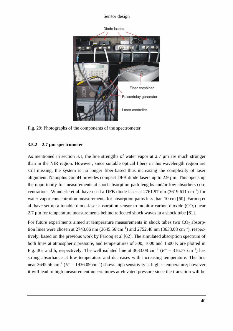
Fig. 29 shows a picture of function generator, laser controller, diode lasers and the fiber com-
biner. The diode lasers, function generator, laser controller, demultiplexing optics, detectors
and data acquisition system are located on a movable table (Thorlabs), which enables conve-
nient equipment transport to experiments situated at different places.
Fig. 28: Schematic drawing and photograph of a fiber-based wavelength-multiplexed diode
laser sensor
Laser 1
Laser 2
Laser 3
Fiber
combiner
Singlemode
fiberIsolator Collimator Collimator
Translation
Stage
Grating
Multiplexed
light
Aspheric
lens
Lens focal point
(at fiber end)
Multimode
fiber
Detector
Spherical
mirror
Combustion device
Laser 4
Detector
Multimode
fiber
Grating
Sensor design
40
Fig. 29: Photographs of the components of the spectrometer
3.5.2 2.7 µm spectrometer
As mentioned in section 3.1, the line strengths of water vapor at 2.7 µm are much stronger
than in the NIR region. However, since suitable optical fibers in this wavelength region are
still missing, the system is no longer fiber-based thus increasing the complexity of laser
alignment. Nanoplus GmbH provides compact DFB diode lasers up to 2.9 µm. This opens up
the opportunity for measurements at short absorption path lengths and/or low absorbers con-
centrations. Wunderle et al. have used a DFB diode laser at 2761.97 nm (3619.611 cm–1
) for
water vapor concentration measurements for absorption paths less than 10 cm [60]. Farooq et
al. have set up a tunable diode-laser absorption sensor to monitor carbon dioxide (CO2) near
2.7 µm for temperature measurements behind reflected shock waves in a shock tube [61].
For future experiments aimed at temperature measurements in shock tubes two CO2 absorp-
tion lines were chosen at 2743.06 nm (3645.56 cm–1
) and 2752.48 nm (3633.08 cm–1
), respec-
tively, based on the previous work by Farooq et al [62]. The simulated absorption spectrum of
both lines at atmospheric pressure, and temperatures of 300, 1000 and 1500 K are plotted in
Fig. 30a and b, respectively. The well isolated line at 3633.08 cm–1
(E” = 316.77 cm–1
) has
strong absorbance at low temperature and decreases with increasing temperature. The line
near 3645.56 cm–1
(E” = 1936.09 cm–1
) shows high sensitivity at higher temperature; however,
it will lead to high measurement uncertainties at elevated pressure since the transition will be
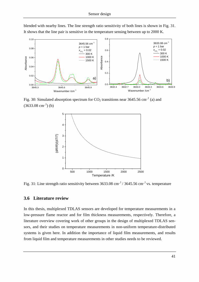
Sensor design
41
blended with nearby lines. The line strength ratio sensitivity of both lines is shown in Fig. 31.
It shows that the line pair is sensitive in the temperature sensing between up to 2000 K.
3645.3 3645.6 3645.9
0.00
0.02
0.04
0.06
0.08
0.10
300 K
1000 K
1500 K
Abso
rba
nce
Wavenumber /cm1
3645.56 cm1
p = 1 bar
xCO
2
= 0.02
a)
3632.4 3632.7 3633.0 3633.3 3633.6 3633.9
0.0
0.2
0.4
0.6
0.8
300 K
1000 K
1500 K
Absorb
ance
Wavenumber /cm1
3633.08 cm1
p = 1 bar
xCO
2
= 0.02
b)
Fig. 30: Simulated absorption spectrum for CO2 transitions near 3645.56 cm–1 (a) and
(3633.08 cm–1) (b)
500 1000 1500 2000 2500
0
1
2
3
4
5
(dR
/R)/
(dT
/T)
Temperature /K
Fig. 31: Line strength ratio sensitivity between 3633.08 cm–1 / 3645.56 cm–1
vs. temperature
3.6 Literature review
In this thesis, multiplexed TDLAS sensors are developed for temperature measurements in a
low-pressure flame reactor and for film thickness measurements, respectively. Therefore, a
literature overview covering work of other groups in the design of multiplexed TDLAS sen-
sors, and their studies on temperature measurements in non-uniform temperature-distributed
systems is given here. In addition the importance of liquid film measurements, and results
from liquid film and temperature measurements in other studies needs to be reviewed.

Sensor design
42
Many researchers have applied multiplexed TDLAS sensors for vapor-phase concentration
and temperature measurements in combustion-related systems in the previous work. Mattison
et al. used a multiplexed TDLAS spectrometer to measure crank-angle-resolved temperature
and water concentration in a homogenous-charge-compression-ignition (HCCI) engine with
wavelength-division multiplexing technique [40]. Baer et al. developed a multiplexed TDLAS
sensor to simultaneously monitor several flow field constituents and properties along a single
path to achieve combustion control, emissions monitoring, atmospheric studies and process
control [63]. Ebert et al. demonstrated a spectrometer with two DFB diode lasers and one Fa-
bry-Perot diode laser to simultaneously measure O2, CH4, CO2, H2O concentration and the
temperature in order to ensure a safe ignition procedure of large-scare multi-burner gas-fired
combustion systems [64].
A variety of studies have been done based on two-line thermometry for applications of tem-
perature measurements in homogenous gas-phase distributed systems [12-13, 18-19]. For sys-
tems with inhomogeneous temperature distribution, Zhou et al. used a linear mixing model by
assuming a trapezoidal-shaped temperature profiles to take into account the boundary layer
effect in a Hencken burner [12], Palaghita et al. defined a non-uniformity variable based on
the difference in temperatures measured with two pairs of absorption lines as well as by using
several absorption lines to evaluate temperature non-uniformities [65]. Sanders et al. intro-
duced a novel multi-line thermometry strategy and measured multiple O2 absorption lines to
determine the temperature distribution within an optical path through two static cells at differ-
ent temperatures [44]. Liu et al. have improved the former multi-line thermometry with two
different strategies, the profile fitting and temperature binning technique, and did several si-
mulation studies and laboratory experiments [20]. The latter strategy is applied in this thesis.
Liquid film formation in the sub-millimeter thickness range is common in many practical ap-
plications. A quantitative measurement of liquid film thickness is helpful to optimize the op-
eration of technical devices and to provide validation data for simulations of such processes.
For instance, the characterization of fuel films is required in many situations of engine com-
bustion: Fuel films may be formed on inner walls of the inlet port in port-injected gasoline
engines (e.g. [66]), on piston heads in direct-injection spark-ignition (DISI) engines (e.g.
[67]), or in the intake manifold during cold start [68]. The aim for improvement is to avoid
wall wetting during fuel injection, thus increasing fuel efficiency and simultaneously decreas-
ing pollutant (i.e., unburned hydrocarbon and soot) emissions. Water-based films or water
mist diagnostics are of interest, e.g., in chemical industry [24], fire suppression [69], and, e.g.
steam power generation [22]. In engine-related applications the observation of the dynamic
behavior of liquid water films is also of interest during injection of water-urea solutions into
Sensor design
43
the exhaust pipe for selective catalytic reduction (SCR) of NOx [70], which motivates the
present work of water-film measurements.
Because of their non-intrusiveness, in the past a number of optical techniques have been de-
veloped to measure liquid film thicknesses. Some of these make use of the relative intensity
difference at the detector, of the totally and partially reflected light, respectively, inside the
film as a measurement of film thickness. Hurlburt et al. used the technique of total internal
reflection which occurs at a liquid-vapor interface due to the refractive index difference be-
tween the two phases. Film thickness was measured in a triangulation scheme where the later-
al displacement of a laser beam; reflected off the liquid layer is observed by a camera [71].
Instead of a laser Shedd et al. directed light from a LED through the film-covered wall and
also determined the displacement of the beam [22].
Spectroscopic methods have also been used for the measurement of fluid film thickness: The
fluorescence emitted from hydrocarbon fuel films after excitation in the ultraviolet was ex-
ploited by Kull et al. for two-dimensional imaging [72]. Greszik et al. used a combination of
LIF and spontaneous Raman scattering for imaging water film thickness [73]. The absorption
of blue laser light in a dye-doped liquid was employed by Mouza et al. to measure the thick-
ness of flowing films [23]. Porter et al. quantified the strong absorption bands around 3.4 µm
of liquid hydrocarbon fuels [74] and used a mid-infrared laser-absorption sensor in this wave-
length range to determine the thickness of liquid films of n-dodecane on transparent windows
in the presence of n-decane vapor [75]. The absorption of near infrared (NIR) emission from a
HeNe-laser was used by Wittig et al. to study the wall film behavior in the suction pipe of a
spark ignition engine [21]. As mentioned in chapter 1, liquid film temperature measurements
are also important. Schagen et al. has used a laser-induced luminescence technique to simul-
taneously determine the temperature distribution and film thickness in wavy liquid films [24],
Alderfer et al. performed sub-microsecond temperature measurement in liquid water using
laser-induced thermal acoustics [76].
In the present work, we apply the introduced temperature-binning technique [44] to resolve
the non-uniform temperature distribution inside a low-pressure flat-flame reactor. Meanwhile,
we setup a novel multi-line TDLAS sensor in the NIR region to simultaneous measure the
liquid water film thickness, temperature and vapor-phase temperature above the film during
film evaporation. To our knowledge, it is the first time to use diode laser absorption technique
to measure liquid water film temperature.

Sensor design
44
Water-vapor temperature sensing in a low-pressure flame reactor
45
4 Water-vapor temperature sensing in a low-pressure flame
reactor
Two different diagnostic methods were compared to determine the spatially-resolved tem-
perature information inside a low-pressure premixed-flame reactor for nanoparticle synthesis.
One method is tunable diode laser absorption spectroscopy (TDLAS) of water vapor, where
the temperature distribution can be obtained by assuming the temperature to be constant in
variable lengths along the line-of-sight (LOS, section 2.5.2). The length fraction of postulated
temperature bins along the LOS is determined. The TDLAS temperature binning technique is
first validated on a premixed atmospheric-pressure burner that has a two-zone temperature
distribution to infer the measurement accuracy and then applied in the lower-pressure reactor.
In the reactor, the other method multi-line NO-LIF imaging was used to validate the spatial
temperature distributions deduced from H2O TDLAS.
4.1 Introduction
Nanosized semiconducting metal oxide particles including ZnO, SnO2, and TiO2 are widely
used for gas-sensing devices, photocatalysis and (opto)electronic devices. A promising route
for the synthesis of these particles is combustion synthesis from evaporated metal-organic
precursors in low-pressure premixed flames [77]. Temperature is an important factor that in-
fluences the properties of the synthesized particles. Therefore, the temperature distribution
inside the low-pressure premixed-flame reactor for nanoparticle synthesis must be known to
simulate the particle formation and growth. For further studies, more specific information is
of great interest, e.g. the effect of the three-dimensional structure of the flame (flame symme-
try) on the particle growth process. Therefore, three-dimensional temperature distribution is
necessary to be determined in such flames.
H2O TDLAS
Laser-based diagnostic techniques are widely used for in-situ non-intrusive temperature mea-
surements in flames [4]. In previous work TDLAS two-line thermometry with a single laser
(laser 1) was used to infer the temperature inside the reactor [78]. This strategy can only pro-
vide LOS-averaged temperature information through the sample by assuming a homogenous
temperature distribution along the path. In general, temperature varies along the beam path in
the reactor due to inhomogeneous mixing flows, heat conduction near chamber walls, and
boundary layer effects, etc. Previous research has been done to correct for such non-uniform-
ities, e.g., the effect from boundary layers [45, 79], the sensitivities to flow non-uniformities
Water-vapor temperature sensing in a low-pressure flame reactor
46
[80], and to infer the path-averaged temperature via different line pairs with different tem-
perature sensitivities [81].
In this thesis the temperature binning technique first demonstrated by Sanders et al. [44] is
applied to obtain the non-uniform temperature distribution inherent in the investigated reactor.
As introduced in section 2.5.2, the length fraction in each specified temperature bin can be
determined by postulated temperature bins with assumed known and uniform pressure and
species mole fraction. However, no information is obtained with respect to the way in which
the constant temperature sections are distributed along the beam path [44]. The technique has
two main advantages: It is fast data evaluation process, because a system of linear equations is
solved and only little knowledge of the temperature distribution in the system is required. The
major drawback is that the result will be too coarse unless many bins are used. However, the
number of probed transitions is limited by the number of laser sources, too many bins can
result in an ill-conditioned problem (cf. chapter 2.5.2) [44].
The four DFB diode lasers (laser 1–4) employed here were used in our lab for previous work,
e.g., temperature measurements in a flat-flame burner and a shock tube. They were first cho-
sen by Mattison et al. [57] and have been listed in Table 2. The five water-vapor lines have
lower state energies E” from 446.5 to 3319.4 cm–1
which are sensitive enough for the applica-
tion in the reactor with a temperature range of 300–2000 K. The temperature distribution
along the absorption path is obtained iteratively using estimated temperature bins along in-
itially unknown length sections through the gas sample. From evaluating the temperature pro-
file with this method at a fixed height position in the flame, TDLAS yields a coarse one-
dimensional temperature profile that indicates the lengths of the paths within the different
temperature regions but without information about their sequence and orientation. Here, we
assume temperature is symmetrically monotonous distributed from the center towards the wall.
Thus, by scanning the laser beam parallel to the burner plate a two-dimensional temperature
distribution can be determined at a fixed height position in the flame. Repeating this proce-
dure at different heights above the burner (HAB), three-dimensional temperature information
can be finally obtained.
In Fig. 32, the simulated spectrum based on the spectroscopic parameters listed in HITRAN
2004 [16] for these five water vapor transitions with different temperature dependence (i.e.,
different lower state energy E”) for the conditions in the atmospheric pressure flame and the
low-pressure reactor are plotted. The black lines are for the methane/air flame at atmospheric
pressure (for water vapor mole fraction: 0.19, optical pathlength: 20 cm, temperature 1000 K).
The red dashed lines are for the low-pressure flame reactor (for water vapor mole fraction:
0.30, optical pathlength: 40 cm, reactor pressure 30 mbar, temperature 1000 K). The simula-
tion in the atmospheric-pressure burner shows that all five transitions show absorbance values

Water-vapor temperature sensing in a low-pressure flame reactor
47
that are larger than 5%. However, for the low pressure reactor, it reveals that water-vapor line
4 and 5 has absorbance values that are larger than 10%, whereas lines 1 and 3 are smaller than
5% since they are more sensitive at even higher temperatures. Liu et al. have developed an
important line selection guideline for the temperature binning technique [20]. For instance,
with a narrow range of E” will not guarantee a good least square fitting for eq. 58.
7153.0 7153.5 7154.0 7154.5 7155.0 7155.5 7156.0
0.0
0.1
0.2
0.3
0.4
0.5
Line 2
Line 1
Atmospheric-pressure burner
Low-pressure reactor
Ab
so
rba
nce
Wavenumber /cm1
6807.0 6807.5 6808.0 6808.5 6809.0
0.0
0.1
0.2
0.3
0.4
0.5
Absorb
ance
Wavenumber /cm1
Line 3
Atmospheric-pressure burner
Low-pressure reactor
7185.0 7185.5 7186.0 7186.5 7187.0
0.0
0.1
0.2
0.3
0.4
0.5
0.6
0.7
0.8
0.9
1.0Line 4
Atmospheric-pressure burner
Low-pressure reactor
Absorb
ance
Wavenumber /cm1
7389.0 7389.5 7390.0 7390.5 7391.0
0.0
0.1
0.2
0.3
0.4
0.5
Line 5
Atmospheric-pressure burner
Low-pressure reactor
Absorb
ance
Wavenumber /cm1
Fig. 32: Simulation of H2O absorption lines for the five transitions for atmospheric-pressure
burner and low-pressure reactor
Multi-line NO-LIF imaging
The diagnostic method of multi-line nitric-oxide (NO) laser-induced fluorescence (LIF) ther-
mometry [8, 82-83] was applied to validate the TDLAS experiments. LIF is a process of spon-
taneous emission from an excited electronic state populated upon absorption of a laser photon.
Quantitative state population distributions or total population prior to laser excitation, measur-
ing temperature or species concentrations can be determined by this method. Multi-line LIF
thermometry can consecutively probe several ground states with different term energies to
determine the temperature with high temperature sensitivity in a wide temperature range.
With this multi-line scanning method, lineshape effects caused by only partial overlap of exci-
Water-vapor temperature sensing in a low-pressure flame reactor
48
tation and absorption lines as well as background contributions are taken into account during
numerical simulations of excitation spectra. Since NO is stable at a wide temperature range
(250–2500 K) and provides strong red-shifted fluorescence signals, NO-LIF thermometry is
attractive [78, 82]. The fundamentals of NO-LIF thermometry have been described previously
[8, 82-83]. A pulsed, tunable, narrowband laser system was used, together with a spectrally
filtered, gated and intensified CCD camera [78]. The laser is tuned over a part of the absorp-
tion spectrum of the NO molecule and individual fluorescence images are taken by the inten-
sified CCD camera for each excitation wavelength. NO-LIF excitation spectra can then be
obtained for each single pixel for the stack of images. The temperature is determined for each
spatial location in the image plane via a non-linear least-square fitting (Levenberg-Marquardt
algorithm) of simulated to experimentally determined NO-LIF excitation spectra. In the fitting
procedure, the line shape and the exact position of the excitation lines are first determined and
a pixel-by-pixel fit is then performed to obtain the temperature [78]. The technique has been
used in previous work to determine the two-dimensional temperature profile (in planes con-
taining the center line of the flame, i.e. parallel to the main gas flow direction) inside the same
reactor [83].
By placing the excitation laser sheet parallel to the burner head, with different locations of the
burner head relative to the light sheet, three dimensional temperature distributions can be ob-
tained in the flame. The technique is provided to select temperature bins in the horizontal
planes of the flame probed by TDLAS and will also help validating the results from TDLAS
measurements. These NO-LIF measurements inside the reactor were performed by C. Hecht
are described in detail in his PhD thesis [84], the results reported here are for purposes of
comparison and validation with the TDLAS measurements.
4.2 Experimental setup
4.2.1 Atmospheric-pressure burner
The 1.4 µm multiplexed fiber-based diode-laser sensor was first applied on an atmospheric-
pressure burner in order to verify the measurement accuracy of the temperature binning tech-
nique. The experimental setup is depicted in Fig. 33. The atmospheric-pressure burner (45
mm diameter) with a water-cooler porous bronze sinter matrix was used here stabilizing a
premixed stoichiometric methane/air flame. A plate was positioned 20 mm above the burner
to stabilize the flame and the temperature was measured at 15 mm height above the burner.
Since this burner has a two-zone temperature distribution: a uniform high temperature in the
flame zone that can be measured by a thermocouple and an ambient air temperature (~300 K)

Water-vapor temperature sensing in a low-pressure flame reactor
49
at both sides (Fig. 33). The TDLAS calculated temperature distribution can be then compared
with the estimated value.
Fig. 33: Experimental setup for the temperature binning technique of TDLAS on an atmos-
pheric-pressure burner
Four fiber-pigtailed diode lasers (NEL) (laser 1–4) are combined, collimated and transmitted
through the atmospheric pressure. Since laser 1 (1398 nm) and 3 (1392 nm) has only 6 nm
difference in wavelength, in the wavelength demultiplexing technique they cannot be sepa-
rated by a grating. Since the flame is steady, the time division multiplexing (TDM) technique
can here be used. In the case the multiplexed beam passing through the sample is registered
by only one detector, which simultaneously simplifies the experimental setup. Each laser is
scanned by a saw-tooth current ramp of 100 Hz across its targeted absorption transition. The
individual absorbances are calculated by Voigt fits using LabVIEW (National instruments)
program which also controlled the experiment.
4.2.2 Low-pressure flame reactor
The low-pressure nanoparticle flame-synthesis reactor is described in detail in [83]. A sche-
matic drawing with front view (a) and top view (b) through the reactor are shown in Fig. 34.
The top view in Fig. 34(b) is the cross section towards the ICCD camera in Fig. 34(a). The
reaction chamber is 300 mm long with a diameter of 100 mm. A H2/O2/Ar flat flame (with
flows of 600, 800, and 300 sccm, respectively) is stabilized at a total pressure of 30 mbar on a
water-cooled sinter matrix burner, which is horizontally mounted inside the vacuum chamber.
Laser 1
Laser 2
Laser 3
Laser 4
Fiber
combiner
Singlemode
Fiber
Isolator
45 mm
20 mm
Stabilizing plate
Collimator Collection
optics
Flat-flame burnerDetector
180 mm

Water-vapor temperature sensing in a low-pressure flame reactor
50
For NO-LIF a fraction of Ar flow is substituted by a 2% NO/Ar mixture to obtain an overall
concentration of 600 ppm NO.
H2O TDLAS
The experimental setup of TDLAS shown in Fig. 34 (a) is similar to the application in the
atmospheric-pressure burner introduced in section 4.2.1. Two wedged (2°) quartz windows
with a free aperture of 90 mm at two sides of the chamber enable the diode laser beams to
pass through the flame perpendicular to the translation axis of the burner head. The distance
between the inner faces of two quartz windows at both sides is 150 mm. All the dimensions
are marked in Fig. 34(b). The position of the beams was varied in a plane parallel to the burn-
er head. Based on the temperature binning method and the assumption of a symmetric tem-
perature distribution with the highest temperature on the burner axis, multiple parallel mea-
surements provide information about the two-dimensional temperature distribution.
Multi-line NO LIF imaging
For the multi-line NO-LIF thermometry, a Raman-shifted narrowband KrF-excimer laser was
tuned over individual NO absorption lines of the A-X (0,0) -band system around 225 nm,
and an ICCD camera (LaVision) was placed perpendicular to the light sheet taking individual
images for each excitation wavelength. The laser energy was kept low enough to avoid satura-
tion of the NO transitions. LIF excitation spectra were then extracted for each pixel from the
obtained images. The experimental data were then fitted with simulated spectra using LIFSim
[85]. By this procedure temperature images were determined in the plane containing the cen-
terline of the reaction chamber.
In the NO-LIF imaging, the windows at both sides previously used for the TDLAS measure-
ments were used to pass the excitation laser light sheet through the combustion chamber in a
plane parallel to the burner head. A third observation window opposite to the burner head
allows detection of the LIF signal (see Fig. 34(a)). Since the limitation of space in the lab, the
laser light is first reflected by a rectangle mirror in front of the window, and then an ICCD
camera (LaVision) was placed far away to obtain the fluorescence images. Hence, the dimen-
sion of the 2D image obtained by NO-LIF is not round but a rectangle with length 90 mm and
width 50 mm.
Through the movement of the burner head perpendicular to the laser light sheet in the same
plane of the beams of the TDLAS technique to obtain a stack of two-dimensional data sets.
These can be assembled into three-dimensional temperature distributions of the flame. It
should be noted that the flame structure slightly changes whenever the burner head is moved
to a different measurement position due to a variation in the heat losses of the flame gases to
the combustion chamber walls.
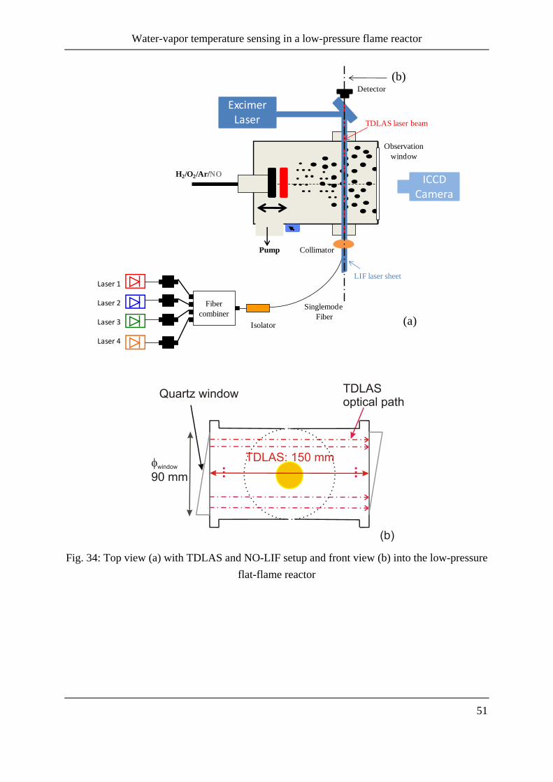
Water-vapor temperature sensing in a low-pressure flame reactor
51
Fig. 34: Top view (a) with TDLAS and NO-LIF setup and front view (b) into the low-pressure
flat-flame reactor
ExcimerLaser
H2/O2/Ar/NO
Laser 1
Laser 2
Laser 3
Laser 4
Fiber
combinerSinglemode
FiberIsolator
Detector
CollimatorPump
Observation
window
ICCDCamera
LIF laser sheet
TDLAS laser beam
(a)
(b)
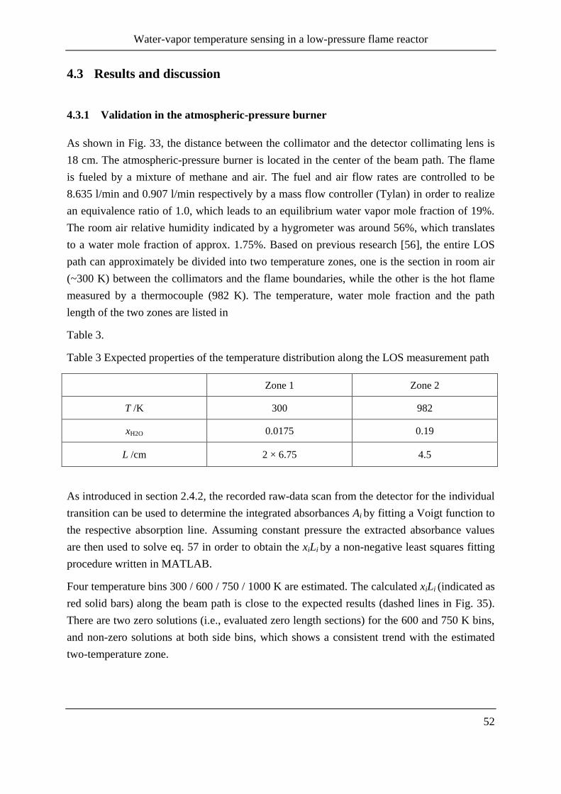
Water-vapor temperature sensing in a low-pressure flame reactor
52
4.3 Results and discussion
4.3.1 Validation in the atmospheric-pressure burner
As shown in Fig. 33, the distance between the collimator and the detector collimating lens is
18 cm. The atmospheric-pressure burner is located in the center of the beam path. The flame
is fueled by a mixture of methane and air. The fuel and air flow rates are controlled to be
8.635 l/min and 0.907 l/min respectively by a mass flow controller (Tylan) in order to realize
an equivalence ratio of 1.0, which leads to an equilibrium water vapor mole fraction of 19%.
The room air relative humidity indicated by a hygrometer was around 56%, which translates
to a water mole fraction of approx. 1.75%. Based on previous research [56], the entire LOS
path can approximately be divided into two temperature zones, one is the section in room air
(~300 K) between the collimators and the flame boundaries, while the other is the hot flame
measured by a thermocouple (982 K). The temperature, water mole fraction and the path
length of the two zones are listed in
Table 3.
Table 3 Expected properties of the temperature distribution along the LOS measurement path
Zone 1 Zone 2
T /K 300 982
xH2O 0.0175 0.19
L /cm 2 × 6.75 4.5
As introduced in section 2.4.2, the recorded raw-data scan from the detector for the individual
transition can be used to determine the integrated absorbances Ai by fitting a Voigt function to
the respective absorption line. Assuming constant pressure the extracted absorbance values
are then used to solve eq. 57 in order to obtain the xiLi by a non-negative least squares fitting
procedure written in MATLAB.
Four temperature bins 300 / 600 / 750 / 1000 K are estimated. The calculated xiLi (indicated as
red solid bars) along the beam path is close to the expected results (dashed lines in Fig. 35).
There are two zero solutions (i.e., evaluated zero length sections) for the 600 and 750 K bins,
and non-zero solutions at both side bins, which shows a consistent trend with the estimated
two-temperature zone.

Water-vapor temperature sensing in a low-pressure flame reactor
53
0 200 400 600 800 1000 1200
0.0
0.2
0.4
0.6
0.8
1.0
Temperature /K
xi*L
i
Expected
Experimental data
Fig. 35: Illustration of the temperature binning results using five individual transitions in the
atmospheric-pressure burner
4.3.2 Low-pressure flame reactor
At low pressure, the linewidth is dominated by Doppler broadening. The reduced collisional
broadening causes narrower transition linewidths in low-pressure than in atmospheric-
pressure environments. Meanwhile, according to eq. 34, the absorbance is also smaller at low
pressure than at atmospheric pressure when species concentration, temperature and pathlength
are identical. However, at low pressure the transitions are more isolated from neighboring
lines, as e.g., for line 2 depicted in Fig. 32.
As suggested in [44], the choice of the temperature bins is critical in the temperature binning
technique. In the present work the temperature profile was first evaluated from the multi NO-
LIF thermometry measurement and, from this information suitable temperature bins were
estimated for evaluating the TDLAS line-of-sight temperature profile. The NO-LIF has an
optical access of 90 mm because of the observation window aperture, while the free beam
path of TDLAS is 150 mm (as shown in Fig. 34b). Hence, the temperature information ob-
tained by NO-LIF should be expanded to a larger region.
In the NO-LIF experiments the gas temperature field was measured by moving the burner
head relative to reference positions for different HAB, thus obtaining a stack of temperature
fields in planes parallel to the burner head for different burner positions. The 2D temperature
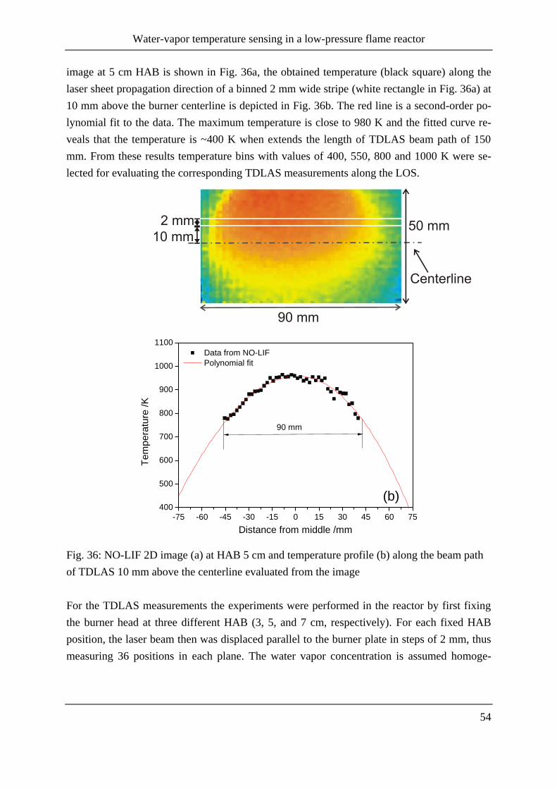
Water-vapor temperature sensing in a low-pressure flame reactor
54
image at 5 cm HAB is shown in Fig. 36a, the obtained temperature (black square) along the
laser sheet propagation direction of a binned 2 mm wide stripe (white rectangle in Fig. 36a) at
10 mm above the burner centerline is depicted in Fig. 36b. The red line is a second-order po-
lynomial fit to the data. The maximum temperature is close to 980 K and the fitted curve re-
veals that the temperature is ~400 K when extends the length of TDLAS beam path of 150
mm. From these results temperature bins with values of 400, 550, 800 and 1000 K were se-
lected for evaluating the corresponding TDLAS measurements along the LOS.
-75 -60 -45 -30 -15 0 15 30 45 60 75
400
500
600
700
800
900
1000
1100
Data from NO-LIF
Polynomial fit
Tem
pera
ture
/K
Distance from middle /mm
90 mm
(b)
Fig. 36: NO-LIF 2D image (a) at HAB 5 cm and temperature profile (b) along the beam path
of TDLAS 10 mm above the centerline evaluated from the image
For the TDLAS measurements the experiments were performed in the reactor by first fixing
the burner head at three different HAB (3, 5, and 7 cm, respectively). For each fixed HAB
position, the laser beam then was displaced parallel to the burner plate in steps of 2 mm, thus
measuring 36 positions in each plane. The water vapor concentration is assumed homoge-

Water-vapor temperature sensing in a low-pressure flame reactor
55
nously distributed along the whole beam path inside the reactor. This is justified because the
flame gases fill the whole chamber due to the absence of an inert gas co-flow.
By these assumptions the length fractions fj for each temperature bin were calculated by eq.
58-61 as shown in Fig. 37. A value of zero on the y-axis indicates the beam crossing the
symmetry axis of the burner, and positive and negative values corresponding to the laser beam
passing above or below this line. The length fraction distribution shows that the flame shape
is asymmetric with respect to the central axis: The maximum of the length fraction of the
highest temperature bin (1000 K) is not located at the zero position. Since the flame is
mounted horizontally, the flame is distorted by buoyancy effects. The evaluated length frac-
tions show that the temperature in the upper part of the plane above the burner is higher than
in the lower part, the location of the highest flame temperature is slightly shifted to the higher
part and distribution of the highest temperature distribution is getting narrower with increas-
ing HAB. It is shown that the high-temperature length fraction is largest (i.e., ~35%) at 3 cm
HAB. The majority of the data points fall within the intermediate temperature bins (550 and
800 K, black circles in Fig. 37), which occupy regions further outside the centerline of the
burner, whereas the higher temperature regions are located in the center region of the respec-
tive planes. As expected, significant length fractions of the low temperature bin (400 K) are
located near the edge of the probed regions. The asymmetric length fraction distribution is
visible for each of the selected temperature bins and all three HAB positions.
To validate the measured spatially resolved water vapor temperature distributions from
TDLAS, the temperature values deduced from the NO-LIF measurements, averaged over a 2
cm stripe along the direction of NIR beam path (as shown in Fig. 36a) were obtained. An ex-
ample for the 5 cm HAB experiment is plotted in Fig. 38. In qualitative agreement with the
TDLAS measurements the temperature profile is also shifted with respect to the burner cen-
terline. Because the flame is asymmetric inside the reactor, TDLAS 2D temperature recon-
struction is impossible. In order to get a symmetric flame, the reactor should be turned to an
upright configuration for further experiments.
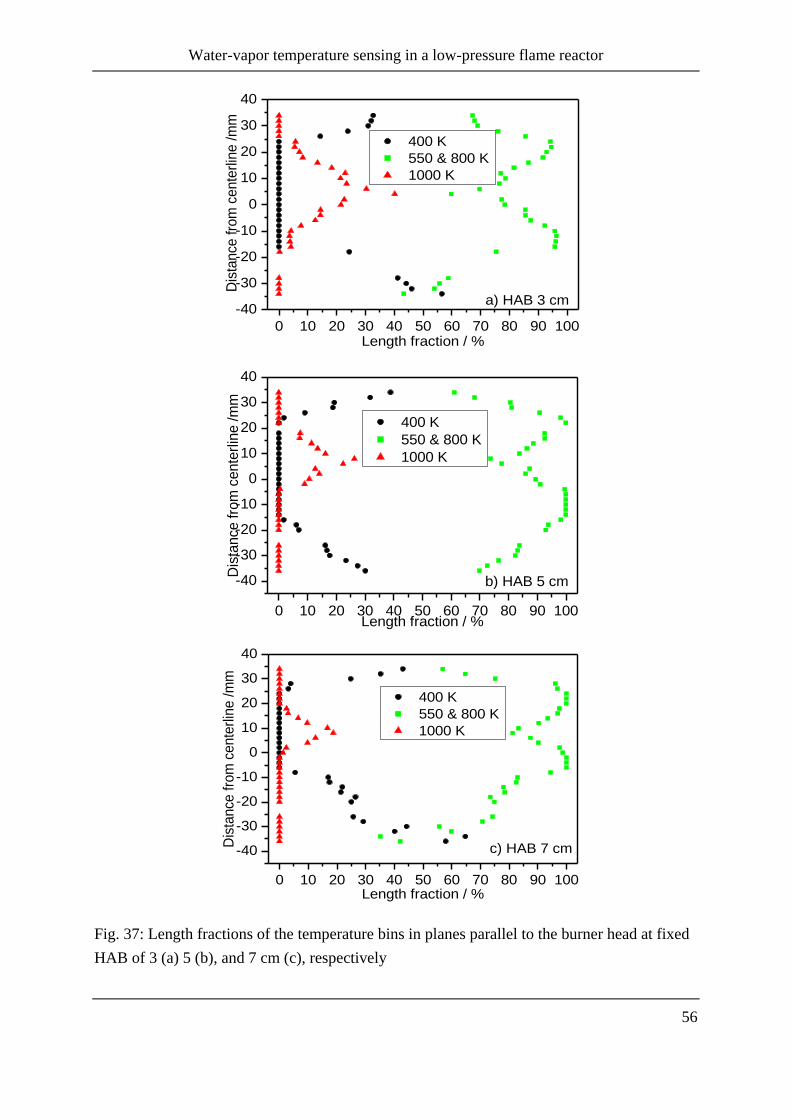
Water-vapor temperature sensing in a low-pressure flame reactor
56
0 10 20 30 40 50 60 70 80 90 100
-40
-30
-20
-10
0
10
20
30
40
a) HAB 3 cm
400 K
550 & 800 K
1000 K
Dis
tance
fro
m c
ente
rlin
e /m
m
Length fraction / %
0 10 20 30 40 50 60 70 80 90 100
-40
-30
-20
-10
0
10
20
30
40
b) HAB 5 cm
400 K
550 & 800 K
1000 K
Dis
tance fro
m c
ente
rlin
e /m
m
Length fraction / %
0 10 20 30 40 50 60 70 80 90 100
-40
-30
-20
-10
0
10
20
30
40
c) HAB 7 cm
400 K
550 & 800 K
1000 K
Dis
tance
fro
m c
ente
rlin
e /m
m
Length fraction / %
Fig. 37: Length fractions of the temperature bins in planes parallel to the burner head at fixed
HAB of 3 (a) 5 (b), and 7 cm (c), respectively
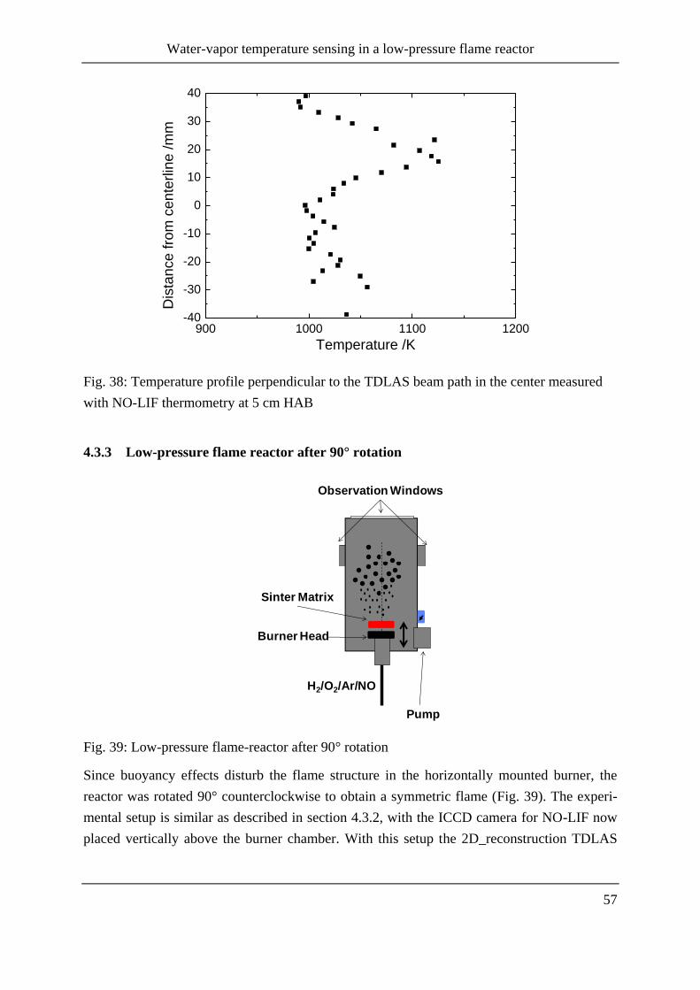
Water-vapor temperature sensing in a low-pressure flame reactor
57
900 1000 1100 1200-40
-30
-20
-10
0
10
20
30
40
Dis
tan
ce
fro
m c
en
terlin
e /
mm
Temperature /K
Fig. 38: Temperature profile perpendicular to the TDLAS beam path in the center measured
with NO-LIF thermometry at 5 cm HAB
4.3.3 Low-pressure flame reactor after 90° rotation
Fig. 39: Low-pressure flame-reactor after 90° rotation
Since buoyancy effects disturb the flame structure in the horizontally mounted burner, the
reactor was rotated 90° counterclockwise to obtain a symmetric flame (Fig. 39). The experi-
mental setup is similar as described in section 4.3.2, with the ICCD camera for NO-LIF now
placed vertically above the burner chamber. With this setup the 2D_reconstruction TDLAS
Observation Windows
H2/O2/Ar/NO
Pump
Sinter Matrix
Burner Head
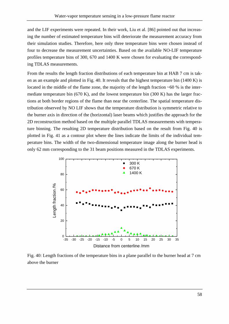
Water-vapor temperature sensing in a low-pressure flame reactor
58
and the LIF experiments were repeated. In their work, Liu et al. [86] pointed out that increas-
ing the number of estimated temperature bins will deteriorate the measurement accuracy from
their simulation studies. Therefore, here only three temperature bins were chosen instead of
four to decrease the measurement uncertainties. Based on the available NO-LIF temperature
profiles temperature bins of 300, 670 and 1400 K were chosen for evaluating the correspond-
ing TDLAS measurements.
From the results the length fraction distributions of each temperature bin at HAB 7 cm is tak-
en as an example and plotted in Fig. 40. It reveals that the highest temperature bin (1400 K) is
located in the middle of the flame zone, the majority of the length fraction ~60 % is the inter-
mediate temperature bin (670 K), and the lowest temperature bin (300 K) has the larger frac-
tions at both border regions of the flame than near the centerline. The spatial temperature dis-
tribution observed by NO LIF shows that the temperature distribution is symmetric relative to
the burner axis in direction of the (horizontal) laser beams which justifies the approach for the
2D reconstruction method based on the multiple parallel TDLAS measurements with tempera-
ture binning. The resulting 2D temperature distribution based on the result from Fig. 40 is
plotted in Fig. 41 as a contour plot where the lines indicate the limits of the individual tem-
perature bins. The width of the two-dimensional temperature image along the burner head is
only 62 mm corresponding to the 31 beam positions measured in the TDLAS experiments.
-35 -30 -25 -20 -15 -10 -5 0 5 10 15 20 25 30 350
20
40
60
80
100
300 K
670 K
1400 K
Length
fra
ction /
%
Distance from centerline /mm
Fig. 40: Length fractions of the temperature bins in a plane parallel to the burner head at 7 cm
above the burner
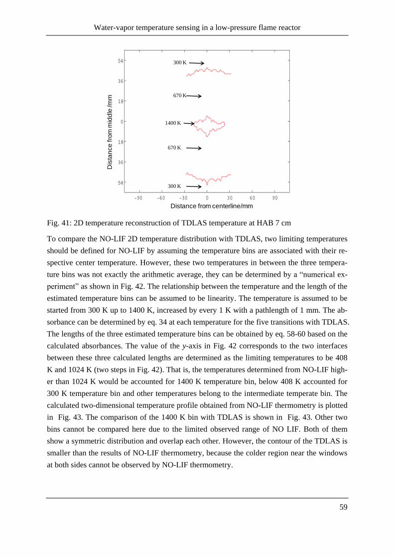
Water-vapor temperature sensing in a low-pressure flame reactor
59
Fig. 41: 2D temperature reconstruction of TDLAS temperature at HAB 7 cm
To compare the NO-LIF 2D temperature distribution with TDLAS, two limiting temperatures
should be defined for NO-LIF by assuming the temperature bins are associated with their re-
spective center temperature. However, these two temperatures in between the three tempera-
ture bins was not exactly the arithmetic average, they can be determined by a “numerical ex-
periment” as shown in Fig. 42. The relationship between the temperature and the length of the
estimated temperature bins can be assumed to be linearity. The temperature is assumed to be
started from 300 K up to 1400 K, increased by every 1 K with a pathlength of 1 mm. The ab-
sorbance can be determined by eq. 34 at each temperature for the five transitions with TDLAS.
The lengths of the three estimated temperature bins can be obtained by eq. 58-60 based on the
calculated absorbances. The value of the y-axis in Fig. 42 corresponds to the two interfaces
between these three calculated lengths are determined as the limiting temperatures to be 408
K and 1024 K (two steps in Fig. 42). That is, the temperatures determined from NO-LIF high-
er than 1024 K would be accounted for 1400 K temperature bin, below 408 K accounted for
300 K temperature bin and other temperatures belong to the intermediate temperate bin. The
calculated two-dimensional temperature profile obtained from NO-LIF thermometry is plotted
in Fig. 43. The comparison of the 1400 K bin with TDLAS is shown in Fig. 43. Other two
bins cannot be compared here due to the limited observed range of NO LIF. Both of them
show a symmetric distribution and overlap each other. However, the contour of the TDLAS is
smaller than the results of NO-LIF thermometry, because the colder region near the windows
at both sides cannot be observed by NO-LIF thermometry.
Distance from centerline/mm
Dis
tan
ce f
rom
mid
dle
/mm
300 K
670 K
1400 K
670 K
300 K
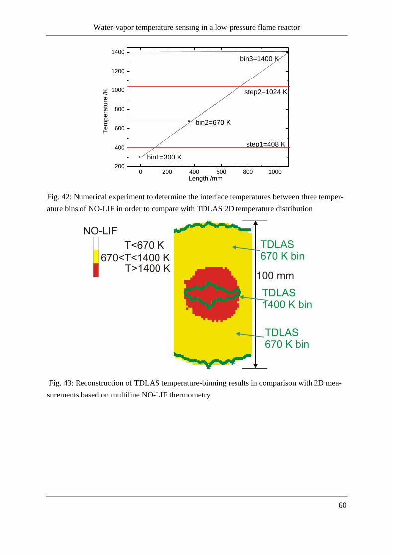
Water-vapor temperature sensing in a low-pressure flame reactor
60
0 200 400 600 800 1000200
400
600
800
1000
1200
1400
step2=1024 K
step1=408 K
bin3=1400 K
bin2=670 K
bin1=300 K
Tem
pera
ture
/K
Length /mm
Fig. 42: Numerical experiment to determine the interface temperatures between three temper-
ature bins of NO-LIF in order to compare with TDLAS 2D temperature distribution
Fig. 43: Reconstruction of TDLAS temperature-binning results in comparison with 2D mea-
surements based on multiline NO-LIF thermometry
Water-vapor temperature sensing in a low-pressure flame reactor
61
4.4 TDLAS temperature measurements: Summary
In this chapter, the TDLAS multi-line thermometry for flames exhibiting a non-uniform tem-
perature distribution along the absorption beam path was investigated. The temperature bin-
ning technique was applied using four diode lasers (lasers 1–4) with five water absorption
transitions of different temperature dependency (i.e., different lower-state energies E”). In
such cases the non-uniform temperature distribution along the line of sight can be obtained by
non-negative least squares fitting.
The technique was first investigated in an atmospheric-pressure burner with a “two-zone”
temperature distribution to provide an estimate for the measurement accuracy. The calculated
product of assumed concentration and length fraction within which concentration is assumed
to be constant, xi Li, was compared with expected values and showed reasonable consistency.
The technique was then applied in a low-pressure flat-flame burner, where a comparison with
results from multi-line NO-LIF thermometry was available, and which provided some initial
estimate for the choice of proper temperature bins (400, 550, 800, and 1000 K, respectively).
Experiments were performed at different HAB (3, 5, and 7 cm, respectively), with the NIR
laser beams routed through the reactor in planes parallel with the burner head at each fixed
HAB position. The length fractions of each temperature bin at each HAB were evaluated from
the absorption signals. The highest temperature was observed at 3 cm HAB. However, since
the burner was mounted horizontally, the 1000 K temperature bin was located off center of
the burner symmetry line, which was an indication that the flame was asymmetric due to
buoyancy effects. After rotating the reactor by 90°, the TDLAS showed (e.g. at HAB 7 cm) a
symmetric temperature distribution. It shows a similar spatial temperature distribution com-
pared to the NO-LIF method.

Water-vapor temperature sensing in a low-pressure flame reactor
62
TDLAS applied for liquid-water film-thickness measurements
63
5 TDLAS applied for liquid-water film-thickness measurements
In this thesis a fiber-based multiplexed tunable diode-laser absorption sensor with four near-
infrared (NIR) distributed-feedback (DFB) diode lasers at ~1.4 µm was used for the first time
for simultaneous non-intrusive measurement of liquid water film thickness, liquid-phase tem-
perature, and vapor-phase temperature above the film, respectively. As detailed in section
2.5.1, the vapor-phase temperature is obtained from the absorbance ratio of two lasers rapidly
tuned across narrow gas-phase absorption transitions, whereas the other parameters are calcu-
lated from the absorbance ratio at three wavelengths assessing the broad-band spectral signa-
ture of liquid water. With regard to the water film temperature measurements an optimized
combination of laser wavelengths were determined using liquid-water absorption cross sec-
tions measured by a Fourier transform infrared (FTIR) spectrometer. When probing the liquid
film at three different wavelengths with significantly different absorption cross-sections, two
of these have extreme different temperature sensitivities, which favors them for liquid tem-
perature measurements. It allows discriminating against additional signal losses due to surface
fowling, reflection and beam steering simultaneously. The performance of the sensor was first
validated in calibration-tool experiments with liquid layers of known thickness and tempera-
ture. Then experiments are presented for time-resolved thickness and temperature measure-
ments of evaporating water films on a transparent quartz plate. The sensor was also applied in
a flow channel for film thickness measurements. The TDLAS technique is also compared
with two imaging diagnostic methods performed within the PhD thesis work of D. Greszik –
laser-induced fluorescence (LIF) from low concentrations of a dissolved tracer substance, and
spontaneous Raman scattering of liquid water, respectively, both excited with a laser beam at
266 nm [87]. Results from each method are compared for the thickness measurement of liquid
water films deposited on a transparent quartz plate.
5.1 Liquid water
In the liquid phase, water exhibits broad-band absorption from the OH-stretch vibrational
bands in the NIR region due to hydrogen bridge bonding and hindered rotations. The vibra-
tional manifolds are broadened significantly due to the high density and the large number of
collisions. Compared to the gas phase the main stretching band in liquid water is shifted to a
lower frequency (v3, 3490 cm–1
and v1, 3280 cm–1
) [88] and the bending frequency increased
(v2, 1644 cm–1
) [89]. The frequency of the fundamental vibration modes for liquid water and
water vapor are shown in Table 4. A review of the absorption spectrum of liquid water cover-
ing the wavelength region between 0.2 and 200 µm is given by Hale et al. [90] and a more

TDLAS applied for liquid-water film-thickness measurements
64
detailed compilation in the 0.65–2.5 µm range was presented by Kou et al. [91]. A portion of
the broad-band liquid water absorption spectrum published by Kou et al is shown in Fig. 44
[91]. The imaginary part of the refractive index of water at room temperature was reported,
however, the measurements were performed in a Bomem DA3.02 FTIR spectrometer with
low spectral resolution of 16 cm–1
[91]. In the present work higher resolution spectra at differ-
ent temperatures were measured in our FTIR spectrometer, which will be described in the
section 5.2.2.
Table 4: Fundamental vibrations and frequencies for water vapor and liquid water [34]
Vibrational mode Frequency in water vapor [cm–1] Frequency in liquid water [cm–1]
v1 3652 3280
v2 1595 1644
v3 3756 3490
4000 5000 6000 7000 8000
-20
0
20
40
60
80
100
120
140
Wavenumber /cm1
Absorp
tion /
cm
Temperature : 22oC
Fig. 44: Absorption spectrum of liquid water from 4000 to 8000 cm–1
[91]
5.2 Measurement strategy
TDLAS relies on a rapid scanning of the laser wavelength via current tuning to distinguish
between narrow band molecular absorption features in the gas phase and laser attenuation due
to other losses such as reflection at interfaces, window fouling, scattering, and beam steering.
TDLAS applied for liquid-water film-thickness measurements
65
When applying to water-vapor measurements, the molecular absorption of gas-phase species
is then derived from the spectrally integrated narrowband absorption features after subtracting
the spectrally unstructured background effects. When a liquid water film is present in the
beam path, additional absorption originating from the unstructured broad overtone and/or
combination vibrational bands in the liquid occurs. Using a suitable combination of different
wavelengths its contribution also is subtracted in the data evaluation when determining the
line-integrated absorption from the gas-phase species. At the same time the data evaluation
can also return information about the broad-band liquid water absorption and thus film thick-
ness. Because in the NIR region (5500–8000 cm–1
) the broad-band absorption of liquid water
is strongly wavelength dependent, a measurement at more than one wavenumber position al-
lows separating the absorption due to liquid water from the other light losses that can be con-
sidered wavelength independent absorption. In addition, the liquid water absorption spectrum
changes with temperature (cf. [92]) in this region, this must be taken into account when de-
termining the film thickness. With a suitable choice of several different wavenumber positions
based on our survey FTIR measurements of liquid water absorption cross sections (see be-
low), the liquid film thickness and its temperature in the presence of unspecific laser attenua-
tion can be simultaneously deduced.
5.2.1 Vapor-phase temperature
As already introduced in chapter 4, TDLAS is commonly used for the measurement of vapor-
phase temperature, Tv, and species concentration [18, 60, 93-94]. For temperature measure-
ments in environments with unknown absorber concentrations a minimum of two transitions
with a separation in ground state energy adjusted to the expected temperature range must be
used [12] taking into account their spectral properties, such as overlap with neighboring tran-
sitions, line strength, lower state energy, thermal population, and line broadening and shifting
[54]. The contribution of broad-band absorbers or the attenuation due to losses on the optics is
excluded by scanning the lasers rapidly across the line profiles and by evaluating the contribu-
tion of the narrow-band absorption only. When measuring water vapor concentration and
temperature above liquid films, the broad-band absorption features of the liquid film add to
the losses and can be neglected from the evaluation of absorbance ratios.
In the experiments presented here, we follow the line selection for the measurement of Tv as
discussed in chapter 3.3 assessing two transitions in the v1+v3 band with transition frequencies
of 7185.59 and 7390.13 cm–1
(denoted as laser 3 and 4 in chapter 3.3, respectively). The va-
por-phase temperature can be then obtained by comparing the absorbance ratio between laser
3 and 4 with two-line thermometry.

TDLAS applied for liquid-water film-thickness measurements
66
5.2.2 Liquid-phase temperature and film thickness
Since in the early research there are no accurate enough liquid-water absorption cross sections
available in the NIR region of interest, in the present thesis a FTIR spectrometer with a spec-
tral resolution of 2 cm–1
was used to measure the wavelength- and temperature- dependent
absorption cross section (v,Tl) of liquid water. For this purpose tri-distilled water was filled
in a 1-mm-pathlength quartz cuvette with two optical windows and a double-jacket wall
through which thermostating oil was circulated with temperatures between 298 and 348 K.
The absorption spectrum at different temperatures is presented in Fig. 45. The error bars indi-
cate a statistical error of 1% for three repeated experiments. With increasing temperature, the
peak of the absorption feature slightly shifts towards larger wavenumbers (i.e., shorter wave-
lengths) [92, 95]. Hence, the temperature of the liquid can thus be retrieved from measured
transmittance ratios at suitably chosen wavelength positions, ideally at both sides of the peak
maximum, where the derivative of absorption cross-sections with respect to temperature,
d/dT has an opposite sign.
6000 6500 7000 75000
100
200
300
400
500
600
700
298 K
298 K
308 K
318 K
328 K
338 K
348 K
Absorp
tion c
ross-s
ection /
cm
2/m
ol
Wavenumber /cm–1
348 K
Fig. 45: Near-infrared absorption spectrum of liquid water in the range 5500–8000 cm–1
for
temperatures between 298 and 348 K measured via FTIR
The d/dT is depicted as a dashed line in Fig. 46. The wavenumbers of the diode lasers used
in the present work are marked as vertical lines. Lasers 3 and 4 are the two used for the vapor
phase temperature measurements (see section 5.2.1). Two additional diode lasers (laser 5 and
laser 6) were positioned around the extrema (7082.89 cm–1
and 6714.57 cm–1
, respectively) of
the d/dT curve. Because laser 4 exhibits the lowest absorption cross-section in the liquid (red
curve shown in Fig. 46), it can be combined with laser 5 and 6 to infer the additional non-
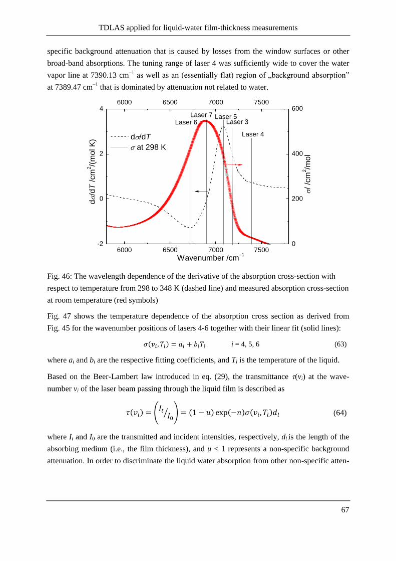
TDLAS applied for liquid-water film-thickness measurements
67
specific background attenuation that is caused by losses from the window surfaces or other
broad-band absorptions. The tuning range of laser 4 was sufficiently wide to cover the water
vapor line at 7390.13 cm–1
as well as an (essentially flat) region of „background absorption”
at 7389.47 cm–1
that is dominated by attenuation not related to water.
6000 6500 7000 7500-2
0
2
4
/
/cm
2/m
ol
Laser 7Laser 3
Laser 4
Laser 5
d/d
T /
cm
2/(
mo
l K
) d/dT
Laser 6
Wavenumber /cm1
6000 6500 7000 7500
0
200
400
600
at 298 K
Fig. 46: The wavelength dependence of the derivative of the absorption cross-section with
respect to temperature from 298 to 348 K (dashed line) and measured absorption cross-section
at room temperature (red symbols)
Fig. 47 shows the temperature dependence of the absorption cross section as derived from
Fig. 45 for the wavenumber positions of lasers 4-6 together with their linear fit (solid lines):
i = 4, 5, 6 (63)
where ai and bi are the respective fitting coefficients, and Tl is the temperature of the liquid.
Based on the Beer-Lambert law introduced in eq. (29), the transmittance (vi) at the wave-
number vi of the laser beam passing through the liquid film is described as
(64)
where It and I0 are the transmitted and incident intensities, respectively, dl is the length of the
absorbing medium (i.e., the film thickness), and u < 1 represents a non-specific background
attenuation. In order to discriminate the liquid water absorption from other non-specific atten-
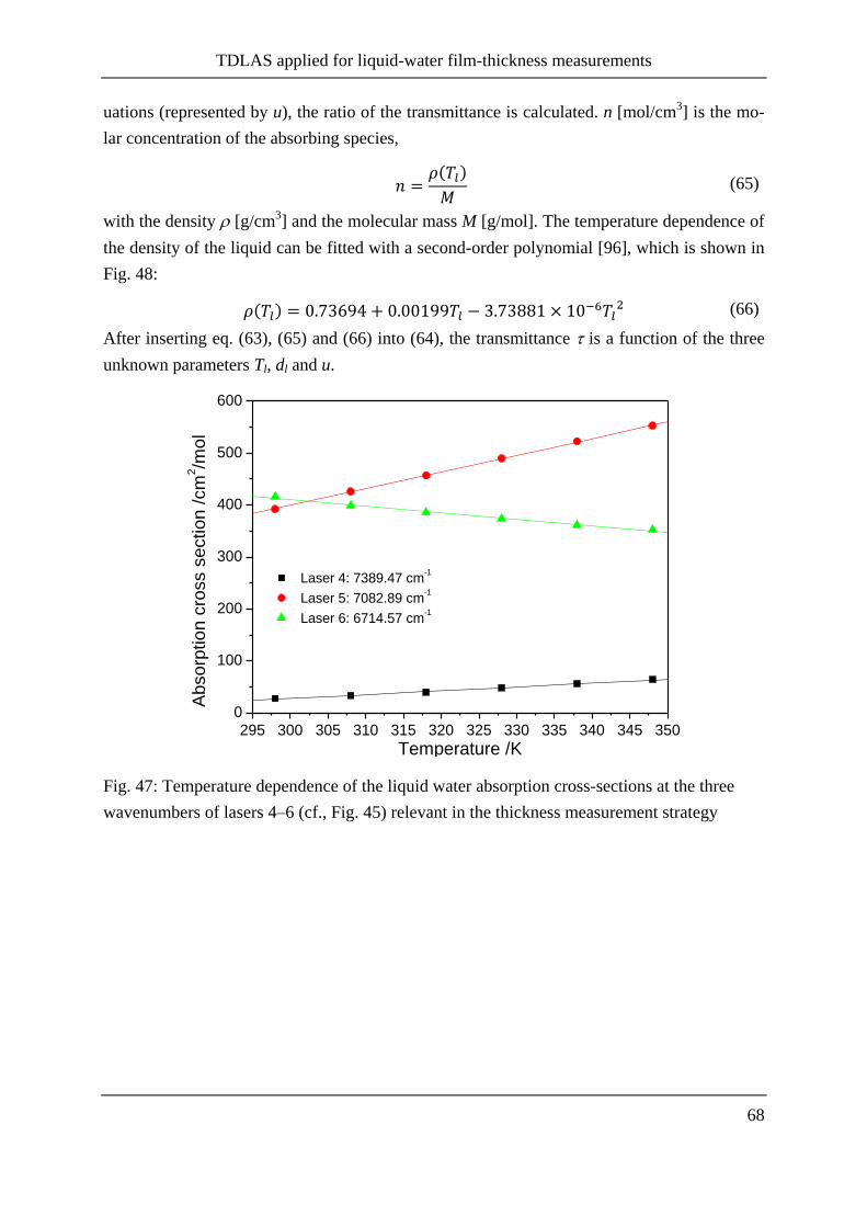
TDLAS applied for liquid-water film-thickness measurements
68
uations (represented by u), the ratio of the transmittance is calculated. n [mol/cm3] is the mo-
lar concentration of the absorbing species,
(65)
with the density [g/cm3] and the molecular mass M [g/mol]. The temperature dependence of
the density of the liquid can be fitted with a second-order polynomial [96], which is shown in
Fig. 48:
(66)
After inserting eq. (63), (65) and (66) into (64), the transmittance is a function of the three
unknown parameters Tl, dl and u.
295 300 305 310 315 320 325 330 335 340 345 350
0
100
200
300
400
500
600
Laser 4: 7389.47 cm-1
Laser 5: 7082.89 cm-1
Laser 6: 6714.57 cm-1
Ab
so
rptio
n c
ross s
ectio
n /
cm
2/m
ol
Temperature /K
Fig. 47: Temperature dependence of the liquid water absorption cross-sections at the three
wavenumbers of lasers 4–6 (cf., Fig. 45) relevant in the thickness measurement strategy
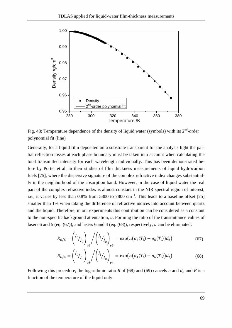
TDLAS applied for liquid-water film-thickness measurements
69
280 300 320 340 360 380
0.95
0.96
0.97
0.98
0.99
1.00
Density /
g/c
m3
Temperature /K
Density
2nd
-order polynomial fit
Fig. 48: Temperature dependence of the density of liquid water (symbols) with its 2nd
-order
polynomial fit (line)
Generally, for a liquid film deposited on a substrate transparent for the analysis light the par-
tial reflection losses at each phase boundary must be taken into account when calculating the
total transmitted intensity for each wavelength individually. This has been demonstrated be-
fore by Porter et al. in their studies of film thickness measurements of liquid hydrocarbon
fuels [75], where the dispersive signature of the complex refractive index changes substantial-
ly in the neighborhood of the absorption band. However, in the case of liquid water the real
part of the complex refractive index is almost constant in the NIR spectral region of interest,
i.e., it varies by less than 0.8% from 5800 to 7800 cm–1
. This leads to a baseline offset [75]
smaller than 1% when taking the difference of refractive indices into account between quartz
and the liquid. Therefore, in our experiments this contribution can be considered as a constant
to the non-specific background attenuation, u. Forming the ratio of the transmittance values of
lasers 6 and 5 (eq. (67)), and lasers 6 and 4 (eq. (68)), respectively, u can be eliminated:
(67)
(68)
Following this procedure, the logarithmic ratio R of (68) and (69) cancels n and dl, and R is a
function of the temperature of the liquid only:
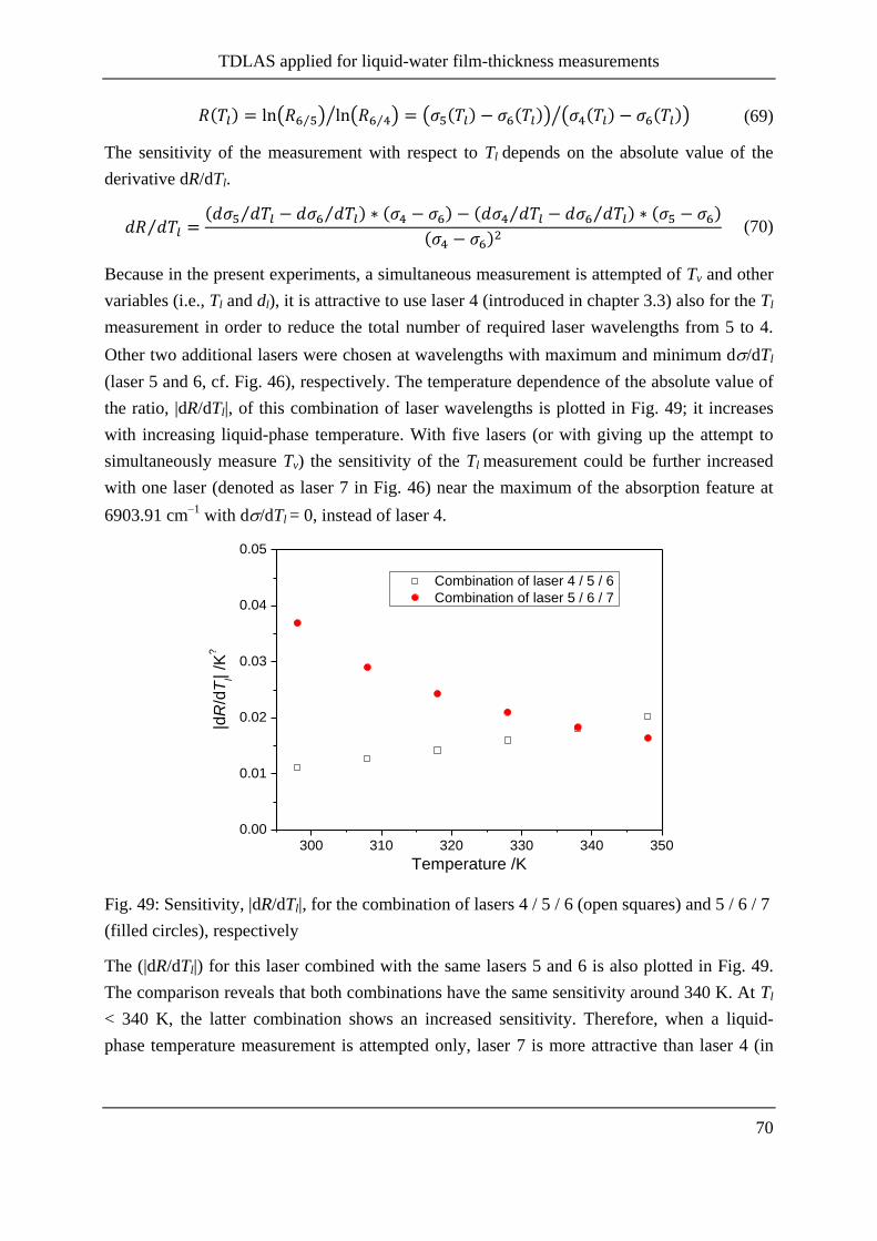
TDLAS applied for liquid-water film-thickness measurements
70
(69)
The sensitivity of the measurement with respect to Tl depends on the absolute value of the
derivative dR/dTl.
(70)
Because in the present experiments, a simultaneous measurement is attempted of Tv and other
variables (i.e., Tl and dl), it is attractive to use laser 4 (introduced in chapter 3.3) also for the Tl
measurement in order to reduce the total number of required laser wavelengths from 5 to 4.
Other two additional lasers were chosen at wavelengths with maximum and minimum d/dTl
(laser 5 and 6, cf. Fig. 46), respectively. The temperature dependence of the absolute value of
the ratio, |dR/dTl|, of this combination of laser wavelengths is plotted in Fig. 49; it increases
with increasing liquid-phase temperature. With five lasers (or with giving up the attempt to
simultaneously measure Tv) the sensitivity of the Tl measurement could be further increased
with one laser (denoted as laser 7 in Fig. 46) near the maximum of the absorption feature at
6903.91 cm–1
with d/dTl = 0, instead of laser 4.
300 310 320 330 340 350
0.00
0.01
0.02
0.03
0.04
0.05
|dR
/dT
l| /K
?
Temperature /K
Combination of laser 4 / 5 / 6
Combination of laser 5 / 6 / 7
Fig. 49: Sensitivity, |dR/dTl|, for the combination of lasers 4 / 5 / 6 (open squares) and 5 / 6 / 7
(filled circles), respectively
The (|dR/dTl|) for this laser combined with the same lasers 5 and 6 is also plotted in Fig. 49.
The comparison reveals that both combinations have the same sensitivity around 340 K. At Tl
< 340 K, the latter combination shows an increased sensitivity. Therefore, when a liquid-
phase temperature measurement is attempted only, laser 7 is more attractive than laser 4 (in
TDLAS applied for liquid-water film-thickness measurements
71
both cases, combined with lasers 5 and 6). However, laser 7 hits a transition with a very large
absorption cross-section, which is not optimal for applications with large film thicknesses.
Therefore, the combination with laser 4 gives a reasonable sensitivity leading to the measure-
ment accuracy discussed later.
When inserting eq. (63) into eq. (69) for the respective laser frequencies, the temperature Tl of
the liquid can be obtained:
(71)
Once Tl is known, dl can be derived when inserting (72) into (68):
(72)
Finally, with the insertion of (72) and (73) into (65), u can be determined from the transmit-
tance measured at the frequency of laser 4:
(73)
The four diode lasers (laser 3‒6) used in the present work are listed in Table 5 with their re-
spective center wavenumber positions and fractional absorptions for a typical liquid film
thickness of 500 µm, and saturated water vapor with 1 cm absorption length at room tempera-
ture, respectively.
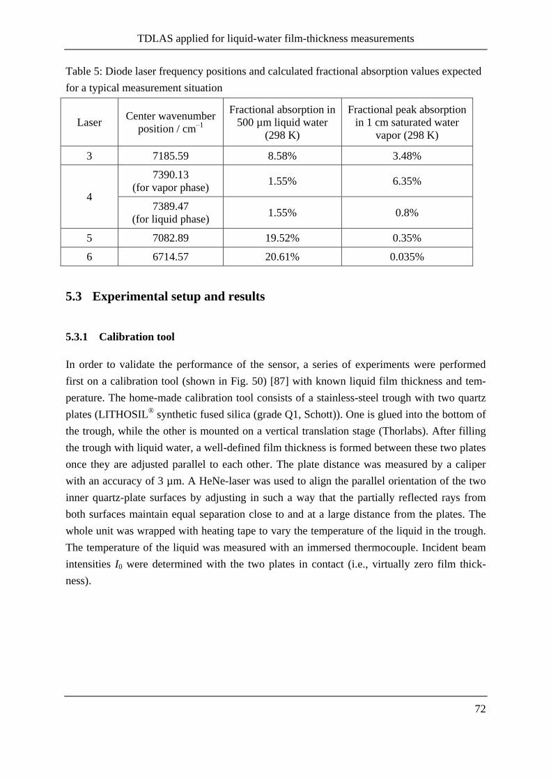
TDLAS applied for liquid-water film-thickness measurements
72
Table 5: Diode laser frequency positions and calculated fractional absorption values expected
for a typical measurement situation
Laser Center wavenumber
position / cm–1
Fractional absorption in
500 µm liquid water
(298 K)
Fractional peak absorption
in 1 cm saturated water
vapor (298 K)
3 7185.59 8.58% 3.48%
4
7390.13
(for vapor phase) 1.55% 6.35%
7389.47
(for liquid phase) 1.55% 0.8%
5 7082.89 19.52% 0.35%
6 6714.57 20.61% 0.035%
5.3 Experimental setup and results
5.3.1 Calibration tool
In order to validate the performance of the sensor, a series of experiments were performed
first on a calibration tool (shown in Fig. 50) [87] with known liquid film thickness and tem-
perature. The home-made calibration tool consists of a stainless-steel trough with two quartz
plates (LITHOSIL®
synthetic fused silica (grade Q1, Schott)). One is glued into the bottom of
the trough, while the other is mounted on a vertical translation stage (Thorlabs). After filling
the trough with liquid water, a well-defined film thickness is formed between these two plates
once they are adjusted parallel to each other. The plate distance was measured by a caliper
with an accuracy of 3 µm. A HeNe-laser was used to align the parallel orientation of the two
inner quartz-plate surfaces by adjusting in such a way that the partially reflected rays from
both surfaces maintain equal separation close to and at a large distance from the plates. The
whole unit was wrapped with heating tape to vary the temperature of the liquid in the trough.
The temperature of the liquid was measured with an immersed thermocouple. Incident beam
intensities I0 were determined with the two plates in contact (i.e., virtually zero film thick-
ness).
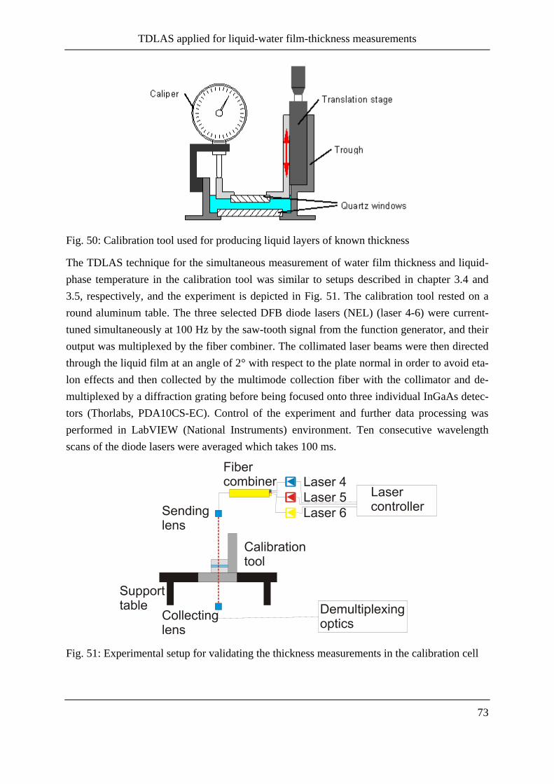
TDLAS applied for liquid-water film-thickness measurements
73
Fig. 50: Calibration tool used for producing liquid layers of known thickness
The TDLAS technique for the simultaneous measurement of water film thickness and liquid-
phase temperature in the calibration tool was similar to setups described in chapter 3.4 and
3.5, respectively, and the experiment is depicted in Fig. 51. The calibration tool rested on a
round aluminum table. The three selected DFB diode lasers (NEL) (laser 4-6) were current-
tuned simultaneously at 100 Hz by the saw-tooth signal from the function generator, and their
output was multiplexed by the fiber combiner. The collimated laser beams were then directed
through the liquid film at an angle of 2° with respect to the plate normal in order to avoid eta-
lon effects and then collected by the multimode collection fiber with the collimator and de-
multiplexed by a diffraction grating before being focused onto three individual InGaAs detec-
tors (Thorlabs, PDA10CS-EC). Control of the experiment and further data processing was
performed in LabVIEW (National Instruments) environment. Ten consecutive wavelength
scans of the diode lasers were averaged which takes 100 ms.
Fig. 51: Experimental setup for validating the thickness measurements in the calibration cell
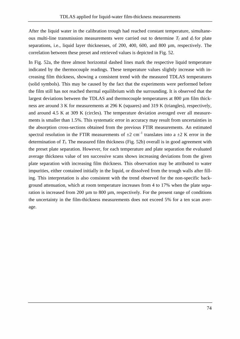
TDLAS applied for liquid-water film-thickness measurements
74
After the liquid water in the calibration trough had reached constant temperature, simultane-
ous multi-line transmission measurements were carried out to determine Tl and dl for plate
separations, i.e., liquid layer thicknesses, of 200, 400, 600, and 800 µm, respectively. The
correlation between these preset and retrieved values is depicted in Fig. 52.
In Fig. 52a, the three almost horizontal dashed lines mark the respective liquid temperature
indicated by the thermocouple readings. These temperature values slightly increase with in-
creasing film thickness, showing a consistent trend with the measured TDLAS temperatures
(solid symbols). This may be caused by the fact that the experiments were performed before
the film still has not reached thermal equilibrium with the surrounding. It is observed that the
largest deviations between the TDLAS and thermocouple temperatures at 800 µm film thick-
ness are around 3 K for measurements at 296 K (squares) and 319 K (triangles), respectively,
and around 4.5 K at 309 K (circles). The temperature deviation averaged over all measure-
ments is smaller than 1.5%. This systematic error in accuracy may result from uncertainties in
the absorption cross-sections obtained from the previous FTIR measurements. An estimated
spectral resolution in the FTIR measurements of ±2 cm–1
translates into a ±2 K error in the
determination of Tl. The measured film thickness (Fig. 52b) overall is in good agreement with
the preset plate separation. However, for each temperature and plate separation the evaluated
average thickness value of ten successive scans shows increasing deviations from the given
plate separation with increasing film thickness. This observation may be attributed to water
impurities, either contained initially in the liquid, or dissolved from the trough walls after fill-
ing. This interpretation is also consistent with the trend observed for the non-specific back-
ground attenuation, which at room temperature increases from 4 to 17% when the plate sepa-
ration is increased from 200 µm to 800 µm, respectively. For the present range of conditions
the uncertainty in the film-thickness measurements does not exceed 5% for a ten scan aver-
age.
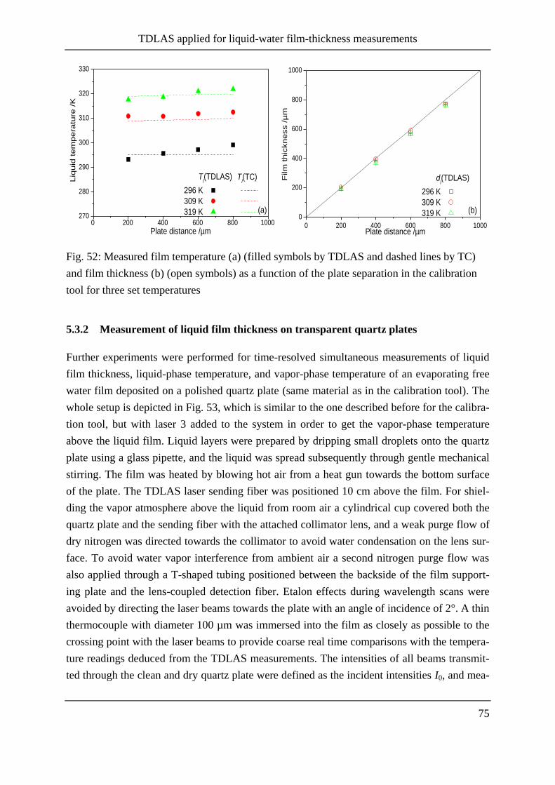
TDLAS applied for liquid-water film-thickness measurements
75
0 200 400 600 800 1000270
280
290
300
310
320
330
(a)
Tl(TC)
Tl(TDLAS)
296 K
309 K
319 K
Liq
uid
tem
pera
ture
/K
Plate distance /µm0 200 400 600 800 1000
0
200
400
600
800
1000
dl(TDLAS)
296 K
309 K
319 K
Film
th
ickn
ess /
µm
Plate distance /µm
(b)
Fig. 52: Measured film temperature (a) (filled symbols by TDLAS and dashed lines by TC)
and film thickness (b) (open symbols) as a function of the plate separation in the calibration
tool for three set temperatures
5.3.2 Measurement of liquid film thickness on transparent quartz plates
Further experiments were performed for time-resolved simultaneous measurements of liquid
film thickness, liquid-phase temperature, and vapor-phase temperature of an evaporating free
water film deposited on a polished quartz plate (same material as in the calibration tool). The
whole setup is depicted in Fig. 53, which is similar to the one described before for the calibra-
tion tool, but with laser 3 added to the system in order to get the vapor-phase temperature
above the liquid film. Liquid layers were prepared by dripping small droplets onto the quartz
plate using a glass pipette, and the liquid was spread subsequently through gentle mechanical
stirring. The film was heated by blowing hot air from a heat gun towards the bottom surface
of the plate. The TDLAS laser sending fiber was positioned 10 cm above the film. For shiel-
ding the vapor atmosphere above the liquid from room air a cylindrical cup covered both the
quartz plate and the sending fiber with the attached collimator lens, and a weak purge flow of
dry nitrogen was directed towards the collimator to avoid water condensation on the lens sur-
face. To avoid water vapor interference from ambient air a second nitrogen purge flow was
also applied through a T-shaped tubing positioned between the backside of the film support-
ing plate and the lens-coupled detection fiber. Etalon effects during wavelength scans were
avoided by directing the laser beams towards the plate with an angle of incidence of 2°. A thin
thermocouple with diameter 100 µm was immersed into the film as closely as possible to the
crossing point with the laser beams to provide coarse real time comparisons with the tempera-
ture readings deduced from the TDLAS measurements. The intensities of all beams transmit-
ted through the clean and dry quartz plate were defined as the incident intensities I0, and mea-

TDLAS applied for liquid-water film-thickness measurements
76
surements were carried out until disturbances by beam steering occurred when the films were
strongly distorted due to surface tension effects.
Fig. 53: Experimental setup of liquid film measurement on a transparent quartz plate
Fig. 54 shows the results from the simultaneous time-resolved measurement of the liquid
layer thickness (blue triangles), the temperature of the liquid (red circles: TDLAS, open
squares: thermocouple (TC)) and the vapor-phase (green diamonds), respectively, for an eva-
porating open water film deposited on the heated quartz plate. Because the data acquisition
time step for the thermocouple reading is 2 s, the other measured parameters were calculated
as an average value for 200 consecutive scans at the 100 Hz repetition rate of the TDLAS
spectrometer. To not overload the figure only every tenth data point is plotted. For ten re-
peated measurements the RMS deviation for the measurement of liquid film thickness and
temperature is 1.5% and 0.5 K, respectively.
At the start of the evaporation process, the temperature of the liquid is around 295 K and then
slowly increases during the first five minutes after data acquisition, before reaching a plateau
region at around 332 K for the following 18 minutes. During the initial heating period the film
thickness slightly decreases from about 1400 µm to around 1210 µm. In the constant tempera-
ture phase the liquid layer thickness linearly decreases until about 300 µm (after 22 min). This
behavior can be understood from a simple model of film evaporation off surfaces, as de-
scribed by the empirical equation [97]:
(74)
Here, g [kg/h] is the mass flux of liquid water leaving the surface area A [m2] of the liquid as
vapor, and [kg/m2h] represents the evaporation coefficient, which for an assumed quiescent
atmosphere above the liquid is a constant with a value of 25. xs [kg/kg] is the humidity ratio in

TDLAS applied for liquid-water film-thickness measurements
77
saturated air at the same temperature as the water surface (at 332 K, xs = 0.155), and x [kg/kg]
is the given humidity ratio of the surrounding air (0.0175 during the experimental run). For
the simulation the initial film thickness was given by 1.22 mm, when the liquid temperature
starts to remain at a constant value of 332 K, as indicated by the thermocouple measurements
(open squares in Fig. 54). It can be observed that the trend calculated from eq. 74 (solid line)
is consistent with the linear decrease of the evaluated TDLAS data.
0 5 10 15 20
260
280
300
320
340
360
0
300
600
900
1200
1500
Film
th
ickn
ess /
µm
Te
mp
era
ture
/K
Time /min
Fig. 54: Time-resolved measurement of film thickness (filled blue triangles), liquid-phase
temperature (filled red circles) and vapor-phase temperature (filled green diamonds) during
film evaporation. Open squares: Thermocouple measurement in the liquid film
For the determination of vapor-phase temperatures, ten consecutive measurements of laser 3
and 4 were averaged and fitted by Voigt functions before the vapor-phase temperature can be
inferred by forming the ratios (eq. (56) in section 2.5.1). The averaged vapor temperature and
RMS error for every 2 s during the experimental run is shown in Fig. 54 (green diamonds). At
the start of film evaporation the measurement uncertainty is 4% (±10 K). This error is the re-
sult of the relatively strong background absorption due to the presence of a thick liquid water
layer at the start of the experiment, which at the given laser power reduces the intensity of the
transmitted signal for the vapor phase measurements, thus decreasing the signal-to-noise ratio
for the scanned absorption lines. This effect can be seen in Fig. 55, where the average from
ten consecutive scans are plotted for each water vapor absorption line accessible by laser 1
and 2, respectively, at 6 min (bottom) and 20 min (top) after start of film evaporation. Also
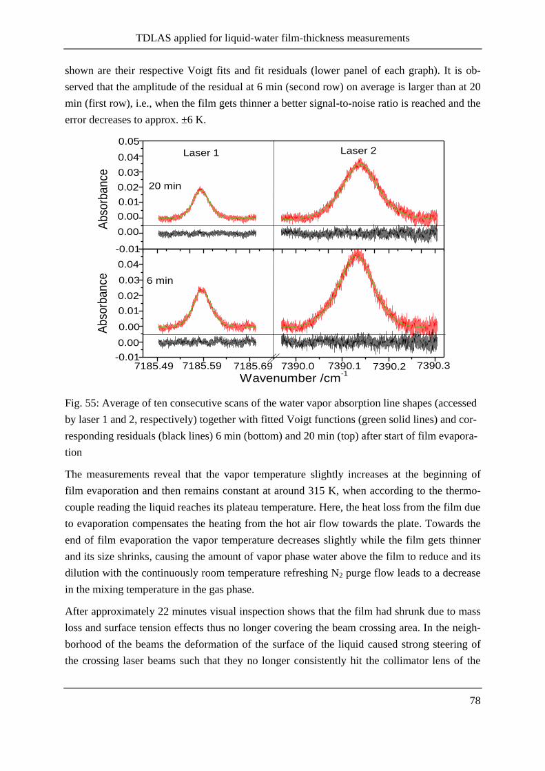
TDLAS applied for liquid-water film-thickness measurements
78
shown are their respective Voigt fits and fit residuals (lower panel of each graph). It is ob-
served that the amplitude of the residual at 6 min (second row) on average is larger than at 20
min (first row), i.e., when the film gets thinner a better signal-to-noise ratio is reached and the
error decreases to approx. ±6 K.
7390.07185.69
6 min
7390.37390.1 7390.27185.49
Abso
rbance
Wavenumber /cm-1
7185.59
Abso
rbance
20 min
0.05
0.04
0.03
0.02
0.01
0.00
-0.01
Laser 2Laser 1
0.00
0.04
0.03
0.02
0.01
0.00
-0.01
0.00
Fig. 55: Average of ten consecutive scans of the water vapor absorption line shapes (accessed
by laser 1 and 2, respectively) together with fitted Voigt functions (green solid lines) and cor-
responding residuals (black lines) 6 min (bottom) and 20 min (top) after start of film evapora-
tion
The measurements reveal that the vapor temperature slightly increases at the beginning of
film evaporation and then remains constant at around 315 K, when according to the thermo-
couple reading the liquid reaches its plateau temperature. Here, the heat loss from the film due
to evaporation compensates the heating from the hot air flow towards the plate. Towards the
end of film evaporation the vapor temperature decreases slightly while the film gets thinner
and its size shrinks, causing the amount of vapor phase water above the film to reduce and its
dilution with the continuously room temperature refreshing N2 purge flow leads to a decrease
in the mixing temperature in the gas phase.
After approximately 22 minutes visual inspection shows that the film had shrunk due to mass
loss and surface tension effects thus no longer covering the beam crossing area. In the neigh-
borhood of the beams the deformation of the surface of the liquid caused strong steering of
the crossing laser beams such that they no longer consistently hit the collimator lens of the
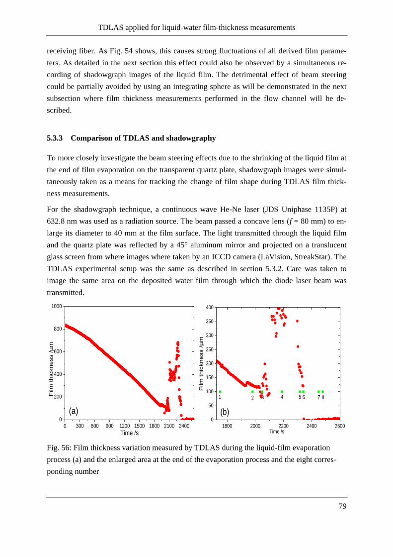
TDLAS applied for liquid-water film-thickness measurements
79
receiving fiber. As Fig. 54 shows, this causes strong fluctuations of all derived film parame-
ters. As detailed in the next section this effect could also be observed by a simultaneous re-
cording of shadowgraph images of the liquid film. The detrimental effect of beam steering
could be partially avoided by using an integrating sphere as will be demonstrated in the next
subsection where film thickness measurements performed in the flow channel will be de-
scribed.
5.3.3 Comparison of TDLAS and shadowgraphy
To more closely investigate the beam steering effects due to the shrinking of the liquid film at
the end of film evaporation on the transparent quartz plate, shadowgraph images were simul-
taneously taken as a means for tracking the change of film shape during TDLAS film thick-
ness measurements.
For the shadowgraph technique, a continuous wave He-Ne laser (JDS Uniphase 1135P) at
632.8 nm was used as a radiation source. The beam passed a concave lens (f = 80 mm) to en-
large its diameter to 40 mm at the film surface. The light transmitted through the liquid film
and the quartz plate was reflected by a 45° aluminum mirror and projected on a translucent
glass screen from where images where taken by an ICCD camera (LaVision, StreakStar). The
TDLAS experimental setup was the same as described in section 5.3.2. Care was taken to
image the same area on the deposited water film through which the diode laser beam was
transmitted.
0 300 600 900 1200 1500 1800 2100 2400
0
200
400
600
800
1000
F
ilm
th
ickn
ess /
µm
Time /s
(a)
1800 2000 2200 2400 2600
0
50
100
150
200
250
300
350
400
Film
th
ickn
ess /
µm
8765432
1
Time /s
(b)
Fig. 56: Film thickness variation measured by TDLAS during the liquid-film evaporation
process (a) and the enlarged area at the end of the evaporation process and the eight corres-
ponding number

TDLAS applied for liquid-water film-thickness measurements
80
The film thickness evaluated from the TDLAS measurements is plotted vs. time in Fig. 56. It
is observed that the film thickness monotonously decreases during the first 1800 s after the
start of the experiment, after which large irregularities in the retrieved values appear (shown
in the enlarged area from 1700 to 2600 s in Fig. 56 (b)). Eight specific instances in time
(marked as green dots in Fig. 56(b) were chosen where the recorded shadowgraph images
where investigated in Fig. 57, where a black dot marks the point of transmission of the NIR
laser beams through the film. At 1750 s and 1980 s (instant 1 and 2) the spatial extent of the
film has reduced but its shape did not change, thus obviously not disturbing the TDLAS mea-
surements. From 2050 s (instant 3) on the film started to shrink substantially, and until 2341s
(instant 6), the NIR laser beams are located at the edge of the film thus being refracted out of
the collection angle of the collimating lens with an accompanying large thickness measure-
ment error (cf. Fig. 56). From 2449s (instant 7), the film was totally evaporated at the position
where the laser beam transmitted the plate, thus the thickness is zero. An integrating sphere
will avoid this effect and will be used in the next section.
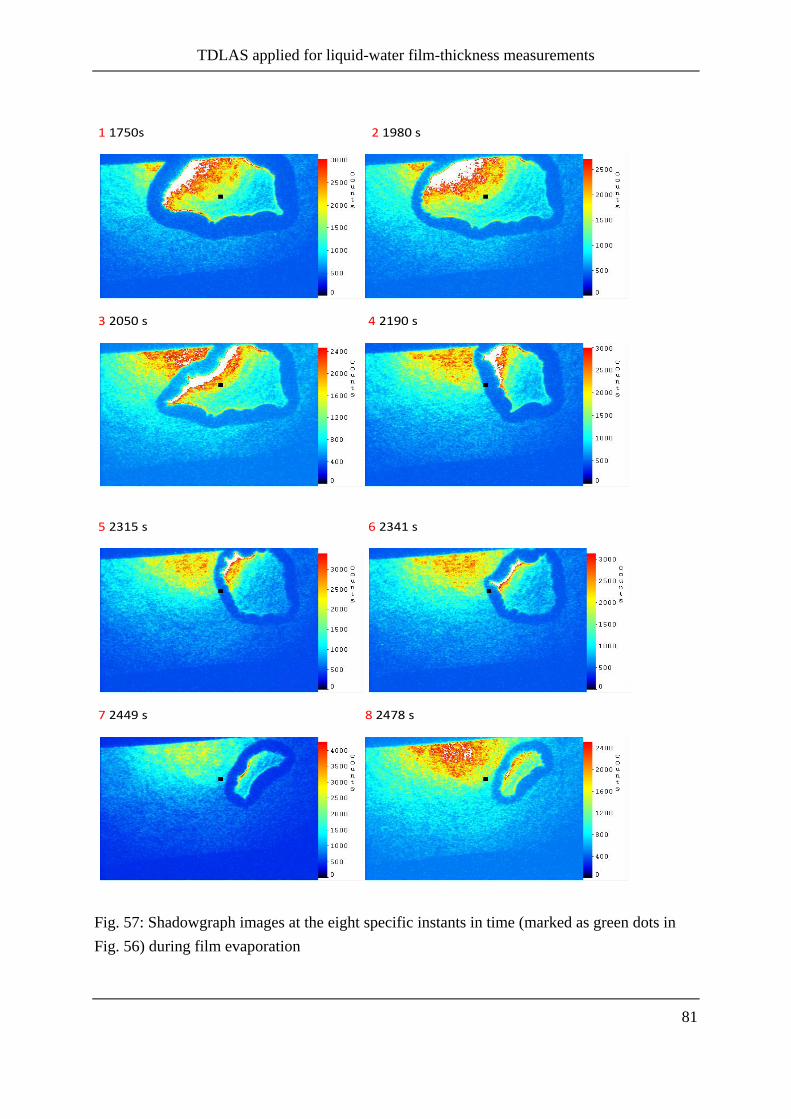
TDLAS applied for liquid-water film-thickness measurements
81
Fig. 57: Shadowgraph images at the eight specific instants in time (marked as green dots in
Fig. 56) during film evaporation
1 1750s 2 1980 s
3 2050 s 4 2190 s
5 2315 s 6 2341 s
7 2449 s 8 2478 s

TDLAS applied for liquid-water film-thickness measurements
82
5.3.4 Measurement of liquid film thickness in a flow channel
The experiments presented in section 5.3.2 on liquid films in an enclosed housing were per-
formed in quiescent atmospheres. However, in many practical applications the measurement
of liquid film thickness in the presence of gas flows above the film is of great interest. For this
purpose a flow channel with rectangular cross section was employed which can provide air
flows of various strength.
The experimental setup for film thickness measurements in the flow channel is shown in Fig.
58. The flow channel consists of four separated aluminum segments with square cross section
of 50 x 50 mm2. The two segments at both ends of the channel are with length 21 cm. There is
an extra honeycomb structure in the first upstream segment of the channel to laminarize the
flow. The two center segments with length 31 cm allow for optical access by transparent
quartz windows in all four sidewalls. A three-hole injection nozzle is inserted into the upper
sidewall which ejects three closely spaced water spray cones onto the lower sidewall used for
film analysis. The air flow velocity in the middle of the channel is to be measured about at
maximum of 7.5 m/s [87].
Fig. 58: Experimental setup for film thickness measurements in a flow channel
The TDLAS spectrometer is operated in the time multiplexing mode. Three diode lasers are
combined and current scanned by a 100 Hz saw-tooth signal during consecutive time spans.
The beams are transmitted through the film. As discussed previously in section 5.3.2 a curved
film surface may refract the transmitted beam such that they will not hit the collimation lens
(5 mm diameter) of the detection fiber. Hence, an integrating sphere (Thorlabs, IS210C) with
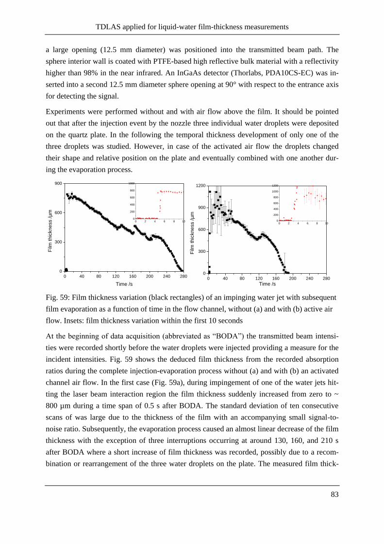
TDLAS applied for liquid-water film-thickness measurements
83
a large opening (12.5 mm diameter) was positioned into the transmitted beam path. The
sphere interior wall is coated with PTFE-based high reflective bulk material with a reflectivity
higher than 98% in the near infrared. An InGaAs detector (Thorlabs, PDA10CS-EC) was in-
serted into a second 12.5 mm diameter sphere opening at 90° with respect to the entrance axis
for detecting the signal.
Experiments were performed without and with air flow above the film. It should be pointed
out that after the injection event by the nozzle three individual water droplets were deposited
on the quartz plate. In the following the temporal thickness development of only one of the
three droplets was studied. However, in case of the activated air flow the droplets changed
their shape and relative position on the plate and eventually combined with one another dur-
ing the evaporation process.
0 40 80 120 160 200 240 280
0
300
600
900
Film
th
ickn
ess /
µm
Time /s
0 2 4 6 8 100
200
400
600
800
1000
0 40 80 120 160 200 240 280
0
300
600
900
1200
Film
th
ickn
ess /
µm
Time /s
0 2 4 6 8 100
200
400
600
800
1000
1200
Fig. 59: Film thickness variation (black rectangles) of an impinging water jet with subsequent
film evaporation as a function of time in the flow channel, without (a) and with (b) active air
flow. Insets: film thickness variation within the first 10 seconds
At the beginning of data acquisition (abbreviated as “BODA”) the transmitted beam intensi-
ties were recorded shortly before the water droplets were injected providing a measure for the
incident intensities. Fig. 59 shows the deduced film thickness from the recorded absorption
ratios during the complete injection-evaporation process without (a) and with (b) an activated
channel air flow. In the first case (Fig. 59a), during impingement of one of the water jets hit-
ting the laser beam interaction region the film thickness suddenly increased from zero to ~
800 µm during a time span of 0.5 s after BODA. The standard deviation of ten consecutive
scans of was large due to the thickness of the film with an accompanying small signal-to-
noise ratio. Subsequently, the evaporation process caused an almost linear decrease of the film
thickness with the exception of three interruptions occurring at around 130, 160, and 210 s
after BODA where a short increase of film thickness was recorded, possibly due to a recom-
bination or rearrangement of the three water droplets on the plate. The measured film thick-
TDLAS applied for liquid-water film-thickness measurements
84
ness decreased to zero at around 275 s after BODA; thus, the whole evaporation process can
be tracked without excessive variations of the transmitted signal intensity, as it was the case in
the previous measurements depicted in Fig. 54 and Fig. 56. Hence, the beam steering effects
occurring when the NIR laser beams are refracted off a changing film surface or during inte-
raction with the film boundaries can be avoided by using the integrating sphere.
For the case with an active air flow above the film the retrieved thickness variation is shown
in Fig. 59b. Also in this case it drastically increased from zero to ~ 1000 µm within the first
0.5 s after BODA. However, in contrast to the case without active air flow the variation in
measured film thickness shows a much stronger fluctuation with a standard deviation of more
than ±100 µm within the first minute after BODA. This might have been caused by small air
bubbles present and vibrate on the surface of the liquid, their movement in the strong air flow
leading to additional beam deflections/deformations not leveled out by the integrating sphere
in front of the detector. When these effects disappeared after approx. 60 s the standard devia-
tion of the measurement decreased to levels similar to the case with no air flow. There also
are visible temporally short increases in film thickness, e.g. around 140 s after BODA –
though much slower than in the case without air flow – which may be ascribed to movement
and/or recombination of the individual water droplets on the surface. The air flow assisted
film evaporation ceased after approx. 180 s after BODA, roughly within 65% of the time it
needed for the case without air flow.
5.3.5 Comparison of TDLAS with tracer LIF and Raman imaging
In collaboration with D. Greszik in our team at IVG the TDLAS technique was compared
with two other nonintrusive diagnostic methods for thickness measurements of liquid water:
tracer LIF and Raman scattering (for details, see [73, 98]). The liquid films were deposited on
the polished quartz plate as described in chapter 5.3.2 (cf. Fig. 60).
Tracer LIF and Raman scattering measurements were performed with a beam from a qua-
drupled Nd:YAG laser at 266 nm with a pulse energy of 9±1 mJ. After a diverging lens the
energy was distributed homogeneously in a circular cross section with a diameter of 30 mm
and passed from below through the quartz plate for excitation of the liquid film (Fig. 60).
After being reflected from an aluminum mirror the backward propagating signal radiation –
either from the tracer fluorescence or from Raman scattering of liquid water – was detected
spatially resolved with an ICCD camera (LaVision, StreakStar) fitted with a UV-lens (Coastal
Optics, 105 mm focal length, f# = 4.5). Fluorescence in the 320–550 nm range was generated
from adding 0.1% by weight of ethyl-acetoacetate (EAA) to the liquid, and was filtered from
scattered and background light by a 320-nm long-pass filter (Schott WG 320). Further sup-
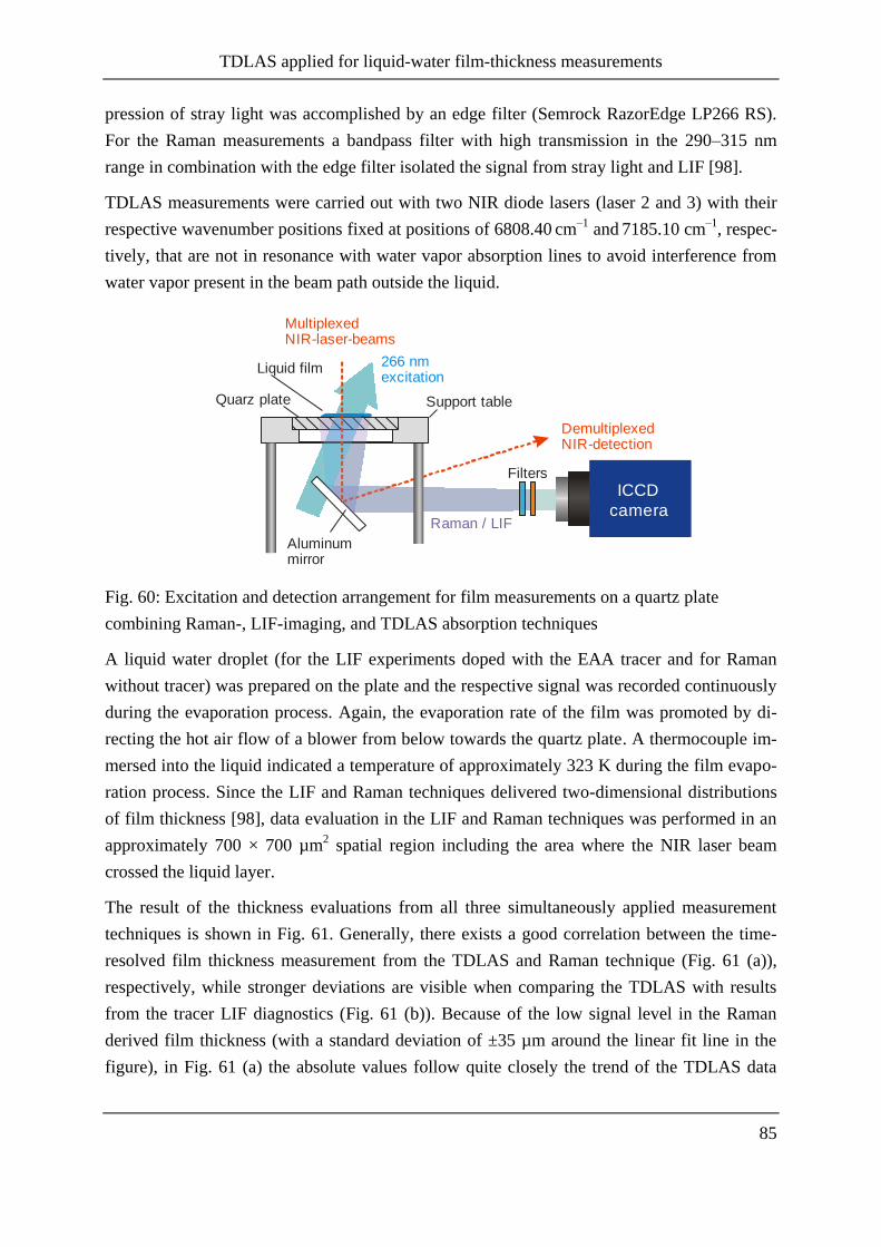
TDLAS applied for liquid-water film-thickness measurements
85
pression of stray light was accomplished by an edge filter (Semrock RazorEdge LP266 RS).
For the Raman measurements a bandpass filter with high transmission in the 290–315 nm
range in combination with the edge filter isolated the signal from stray light and LIF [98].
TDLAS measurements were carried out with two NIR diode lasers (laser 2 and 3) with their
respective wavenumber positions fixed at positions of 6808.40 cm
–1 and
7185.10 cm
–1, respec-
tively, that are not in resonance with water vapor absorption lines to avoid interference from
water vapor present in the beam path outside the liquid.
Raman / LIF
266 nmexcitation
Liquid film
Filters
Aluminummirror
ICCD
camera
MultiplexedNIR-laser-beams
DemultiplexedNIR-detection
Quarz plate Support table
Fig. 60: Excitation and detection arrangement for film measurements on a quartz plate
combining Raman-, LIF-imaging, and TDLAS absorption techniques
A liquid water droplet (for the LIF experiments doped with the EAA tracer and for Raman
without tracer) was prepared on the plate and the respective signal was recorded continuously
during the evaporation process. Again, the evaporation rate of the film was promoted by di-
recting the hot air flow of a blower from below towards the quartz plate. A thermocouple im-
mersed into the liquid indicated a temperature of approximately 323 K during the film evapo-
ration process. Since the LIF and Raman techniques delivered two-dimensional distributions
of film thickness [98], data evaluation in the LIF and Raman techniques was performed in an
approximately 700 × 700 µm2 spatial region including the area where the NIR laser beam
crossed the liquid layer.
The result of the thickness evaluations from all three simultaneously applied measurement
techniques is shown in Fig. 61. Generally, there exists a good correlation between the time-
resolved film thickness measurement from the TDLAS and Raman technique (Fig. 61 (a)),
respectively, while stronger deviations are visible when comparing the TDLAS with results
from the tracer LIF diagnostics (Fig. 61 (b)). Because of the low signal level in the Raman
derived film thickness (with a standard deviation of ±35 µm around the linear fit line in the
figure), in Fig. 61 (a) the absolute values follow quite closely the trend of the TDLAS data

TDLAS applied for liquid-water film-thickness measurements
86
during the whole film evaporation process. On the other hand, during the whole observation
time the measured tracer LIF film thickness is smaller than the TDLAS results and results in a
15% deviation at the end. It is also observed that the measured film thickness deduced from
LIF data decreases much faster than what is evaluated from the TDLAS diagnostic. This phe-
nomenon can be attributed to a preferential evaporation of the tracer from the solution, show-
ing that a suitable tracer still needs to be found for this system. Alternatively, in cases of suf-
ficient signal levels the tracer free diagnostic technique of spontaneous Raman scattering (or
TDLAS) would be more appropriate.
0 60 120 180 240 300 3600
200
400
600
800
1000
1200
(a)
DLAS
Raman scattering
Lin. fit Raman scattering
dl=1017.1-1.7*t
Film
th
ickn
ess /m
Time /s
0 100 200 300 400 500 600 7000
200
400
600
800
1000
1200
(b)
DLAS ratio 1469 / 1392 nm
Tracer LIF
Lin. fit Tracer LIF
dl=1017.06-1.69*t
Film
thic
kness /m
Time /s Fig. 61: Variation of liquid water layer thickness with time during film evaporation deduced,
respectively, from the Raman (a) and LIF (b) signal intensities (open symbols), in comparison
with simultaneously acquired NIR-DLAS ratio measurements (filled symbols). To guide the
eye, the Raman and LIF data, respectively, were fitted with a straight line (red dashed line)
5.4 TDLAS liquid water film thickness measurements: Summary
In this work, a multiplexed TDLAS sensor with a wavelength of ~1.4 µm was employed for
time-resolved measurements of liquid water film thickness. To reliably determine liquid water
film thickness, the absorption strength and the temperature of the liquid must be known accu-
rately. Therefore, absolute absorption cross-sections of liquid water and their temperature
dependence were determined by FTIR spectroscopy within the range of the respective laser
wavelengths. They were first measured with a FTIR spectrometer for liquid temperatures in
the 298–348 K range. Because the liquid-water absorption spectrum shifts towards shorter
wavelengths with increasing temperature, a sensitivity analysis enabled a proper choice of
three wavelengths (lasers 4–6) for an optimized simultaneous measurement of the temperature
of the liquid. This information can be used for correction of the film thickness data obtained
TDLAS applied for liquid-water film-thickness measurements
87
from other line-pair ratios. Probing the liquid film at three wavelengths can eliminate other
non-specific attenuation caused by surface fowling, reflection and beam steering.
The performance of the sensor was first validated in a calibration tool with liquid layers of
known thickness between 200 and 800 µm, and temperatures between 296 and 319 K, respec-
tively. It is found that the uncertainties for the liquid temperature measurement – relative to
the thermocouple readings – are ±1.5%, and for film thickness measurements 5% with respect
to the manually set plate distance.
Experiments were also performed for time-resolved thickness and temperature measurements
of evaporating liquid water films on a transparent quartz plate. The temperatures measured
with TDLAS showed good correlations with simultaneous thermocouple recordings. The liq-
uid temperature increased at the beginning, and remained at a constant level during film eva-
poration as long as thermal equilibrium exists. During film evaporation the thickness linearly
decreased, which was also consistent with a simple model of mass loss by evaporation in a
humid atmosphere. At beginning of film evaporation the vapor-phase temperature determined
by two-line thermometry from the ratio of lasers 3 and 4 has a RMS error of ±10 K due to the
large background absorption from the liquid. The error margin decreased to ±6 K when film
thickness decreased. The temperature of the liquid measured by the thermocouple and
TDLAS correlated well, showing the validity of the optical technique. The vapor-phase tem-
perature increased at the beginning of surface heat up, reached a constant value of 310 K and
decreased towards the end of the evaporation process.
Film thickness measurements were also performed during dynamic film formation, i.e., the
impingement of a water jet on a quartz plate in the presence of an air stream parallel to the
plate. To avoid disturbance of the signal collection due to beam steering caused by distortion
of the film during the impingement and the evaporation, an integrating sphere was installed in
front of the detector. Diode laser control and data readout was done in a time division multip-
lexing (TDM) mode. After deposition the film thickness variation was recorded without and
with active air flow. It is shown that the film decreased much faster with air flow. However,
the accidental presence of air bubbles on the film right after jet impingement caused large
standard deviations for the set of thickness values during this event.
The TDLAS technique was also compared with film thickness imaging techniques developed
in our lab within the thesis of D. Greszik [87] based on tracer LIF (using ethyl acetoacetate as
a fluorescent tracer) and spontaneous Raman scattering, respectively, and simultaneously ap-
plied with the TDLAS technique. The comparison showed a good correlation between the
TDLAS technique and results from Raman scattering. However, film thickness values de-
TDLAS applied for liquid-water film-thickness measurements
88
duced from tracer LIF decreased much faster than results from TDLAS because of preferen-
tial tracer evaporation.
Conclusions and future work
89
6 Conclusions and future work
The main objective of this thesis is to investigate the temperature and liquid film thickness
measurement with fiber-based, multiplexed diode laser absorption spectroscopy (TDLAS)
sensors in combustion-related systems.
6.1 Conclusions
Vapor-phase temperature measurements in combustion-related systems, especially the deter-
mination of temperature in systems with inhomogeneous temperature distribution is of great
interest in practical applications. In this thesis a multiple parallel scanning measurement tech-
nique using several path absorption and temperature binning was employed by monitoring
several absorption lines with different lower state energies and estimating different tempera-
ture bins to infer the temperature distribution along the laser beam path.
In this thesis a ~1.4 µm tunable diode laser absorption spectroscopy (TDLAS) sensor, using
four multiplexed and fiber-coupled DFB diode lasers (lasers 1–4) capable of probing five wa-
ter-vapor absorption lines was set up and applied in a low-pressure flat-flame reactor. The
temperature binning technique was first validated in an atmospheric-pressure flat flame burner
with known temperature profile. When applying the sensor into the low-pressure flat-flame
reactor, it was shown that the flame was asymmetric since the burner was mounted horizontal-
ly. The length fractions of estimated temperature bins evaluated from the TDLAS experiments
by a non-negative least-squares fitting procedure were compared with multi-line NO-LIF
temperature imaging in the same flame environment. After rotating the burner by 90°, the
flame showed a symmetric temperature distribution and TDLAS enabled a 2D temperature
reconstruction. For future applications, simulation for specific line selection should be done
[20] to maximize temperature measurement sensitivity in the temperature range of interest.
Liquid film measurements are crucial in many practical applications. In this thesis, using four
DFB diode lasers (lasers 3–6), the multiplexed TDLAS sensor was applied for the first time
for the simultaneous measurement of the thickness and temperature of liquid water films and
the vapor-phase temperature above the film by using absorption ratios of four individual laser
sources. The developed sensor was first validated in a calibration tool with known film thick-
nesses and temperatures. This resulted in uncertainties of liquid temperature and thickness of
±1.5% and ~5%, respectively. The sensor was then successfully applied for open evaporating
films on a transparent quartz plate and in a flow channel. For the film-thickness measurements
in the flow channel, an integrating sphere was used to reduce the effects of beam steering
when the laser beams traverse the liquid layer with irregular surface topology. This necessi-
Conclusions and future work
90
tated time-multiplexing instead of wavelength multiplexing for evaluating absorbances from
each laser source. The film thickness evaluated from the TDLAS technique was also com-
pared with other laser-based techniques, e.g., tracer-LIF and Raman imaging. Shadowgraphy
was also used to compare with TDLAS in order to investigate the beam-steering effects of
TDLAS. The present thesis is the first realization of a NIR diode-laser absorption technique
for the simultaneous measurement of liquid water film thickness and temperature.
6.2 Future work
In the present work, direct absorption methods with fixed- and scanned-wavelength spectros-
copy were used. With these methods, significant errors occur when the absorption is low and
other noise sources exist. Wavelength-modulation spectroscopy (WMS) was demonstrated to
be another attractive diagnostic technique, which provides better signal-to-noise ratio (SNR)
[55, 99-100]. For WMS, the laser is fast modulated at hundreds of kHz, and the first harmonic
(1f) and second harmonic (2f) of the laser transmission signals are recorded. With 2f detec-
tion, the sensor sensitivity and accuracy are improved. This technique is more sensitive to the
absorption lineshape not only the amplitude, and insensitive to the low-frequency noise. Nor-
malization of 2f signal by 1f signal can minimize the influences from other non-specific atten-
uation and is also calibration free. Therefore, to improve the SNR for the further applications
in the future, WMS is an advantageous tool [55].
Alternative fuels are currently being developed for internal combustion engines. However,
these fuels have different ignition behavior than conventional fuels. Therefore, the ignition
delay time is of great interest. Ignition delay times can be measured in shock tubes. The initial
gas-dynamic temperature behind the shock wave is usually calculated from the shock wave
velocity. However, the temperature history behind the shock wave that is influenced by both,
gas-dynamic effects at long test time as well as the thermochemistry of the reaction is of great
interest. CO2 is the main product of hydrocarbon combustion, as mentioned in section 3.4.2, a
2.7 µm spectrometer for CO2 is developed and that will be applied for the temperature mea-
surements in the shock tube in future.
In this thesis, only pure water liquid film thickness measurement has been studied. Further
research will be done with various aqueous solutions. In practical applications, studies on thin
films are of interest. Hence, future development of this technique for the characterization of
liquid films might focus on other wavelength regions, e.g., in the mid-infrared exhibiting
stronger absorption features with larger liquid water absorption cross-sections. Furthermore,
detection of film thickness in a reflection mode, e.g., with a retro-reflecting surface would be
also studied in the future.
Own publications originating from this thesis
91
7 Own publications originating from this thesis
7.1 Articles in peer-reviewed journals
1. H. Yang, D. Greszik, I. Wlokas, T. Dreier, C. Schulz, "Tunable diode laser absorption
sensor for the simultaneous measurement of water film thickness, liquid- and vapor-phase
temperature", Appl. Phys. B, 104, 21-27 (2011)
2. D. Greszik, H. Yang, T. Dreier, C. Schulz, "Laser-based Diagnostics for the
Measurement of Liquid Water Film Thickness", Appl. Opt. 50, A60-A67 (2011) .
3. H. Yang, D. Greszik, T. Dreier, C. Schulz, "Simulaneous measurement of liquid water
film thickness and vapor temperature using near-infrared tunable diode laser
spectroscopy," Appl. Phys. B 99, 385-390 (2010).
4. D. Greszik, H. Yang, T. Dreier, C. Schulz, "Measurements of water film thickness by
laser-induced fluorescence and Raman imaging", Appl. Phys.B, 102, 123-132 (2010) .
7.2 Non peer-reviewed articles and conference publications
1. H. Yang, D. Greszik, T. Dreier, C. Schulz, "Laser-based diagnostics for water-film
thickness measurements" (Gordon Conference on Laser Diagnostics in Combustion,
Poster, Watervielly, USA, 2011).
2. D. Greszik, H. Yang, T. Dreier, C. Schulz, Measurements of Liquid Film Thickness by
Tracer LIF, Raman Scattering and Diode Laser Absorption Spectroscopy" (Laser
Applications to Chemical, Security, and Environmental Analysis (LACSEA), San Diego,
CA, USA, 2010).
3. C. Hecht, H. Yang, T. Dreier, and Schulz, "In situ Laser Diagnostics of Temperature,
Intermediate Species Concentration and Particle Size in Gas-Phase Nanoparticle
Synthesis" (Laser Applications to Chemical, Security, and Environmental Analysis
(LACSEA), San Diego, CA, USA, 2010).
4. H. Yang, D. Greszik, T. Dreier, C. Schulz, "Diode laser absorption spectroscopy for
liquid film thickness measurement on transparent walls" (Gordon Conference on Laser
Diagnostics in Combustion, Poster, Watervielly, USA, 2009).
5. C. Hecht, H. Yang, T. Dreier, H. Wiggers, C. Schulz, "3-Dimensional temperature
imaging in a low-pressure flame reactor for nanoparticle synthesis using tomographic
tunable diode laser absorption and multi-line nitric-oxide laser-induced fluorescence
Own publications originating from this thesis
92
imaging" (Gordon Conference on Laser Diagnostics in Combustion, Poster, Watervielly,
USA, 2009).
6. H. Yang, C. Hecht, T. Dreier, H. Wiggers, C. Schulz, "3-Dimensional temperature
imaging in a low-pressure reactor for nanoparticle synthesis using tomographic tunable
diode laser absorption and multi-line nitric-oxide laser-induced fluorescence imaging"
(4th
European Combustion Meeting, Vienna, Austria, 2009).
7. H. Yang, C. Hecht, T. Dreier, H. Wiggers, C. Schulz, "3D tempearture imaging in a low-
pressure flame reactor for nanoparticle synthesis using tomographic TDLAS and multi-
line NO LIF" (4th
European Combustion Meeting, Poster, Vienna, Austria, 2009).
8. H. Yang, M. Hartmann, H. Kronemayer, C. Hecht, T. Dreier, C. Schulz, "A multiplexed
diode-laser sensor for temperature measurements in combustion systems" (32nd
International Symposium on Combustion, Poster, Montreal, Canada, 2008)
References
93
8 References
1. C. Schulz, A. Dreizler, V. Ebert, and J. Wolfrum, "Combustion diagnostics," in Springer
handbook of experimental fluid mechanics, C. Tropea, J. Foss, and A. Yarin, eds.
(Springer, Berlin, 2007).
2. V. Ebert, C. Schulz, H. R. Volpp, J. Wolfrum, and P. Monkhouse, "Laser diagnostics of
combustion processes: From chemical dynamics to technical devices," Isr. J. Chem. 39,
1-24 (1998).
3. J. Wolfrum, T. Dreier, V. Ebert, and C. Schulz, "Laser-based combustion diagnostics," in
Encyclopedia of Anlytical Chemistry, R. A. Meyers, ed. (John Wiley & Sons Ltd,
Chichester, 2000).
4. M. G. Allen, "Diode laser absorption sensors for gas dynamic and combustion flows,"
Meas. Sci. Technol. 9, 545-562 (1998).
5. J. A. Silver, and D. J. Kane, "Diode laser measurements of concentration and temperature
in microgravity combustion," Meas. Sci. Technol. 10, 845-852 (1999).
6. E. R. Furlong, D. S. Baer, and R. K. Hanson, "Combustion control and monitoring using
a multiplexed diode-laser sensor system," Proc. Comb. Inst. 26, 2851-2858 (1996).
7. V. Ebert, and J. Wolfrum, "Absorption spectroscopy," in Optical measurements-
techniques and applications, F. Mayinger, and O. Feldmann, eds. (Springer, Heidelberg,
München, 2001), pp. 227-265.
8. H. Kronemayer, W. G. Bessler, and C. Schulz, "Gas-phase temperature imaging in spray
systems using multi-line NO-LIF thermometry," Appl. Phys. B 81, 1071-1074 (2005).
9. C. Schulz, and V. Sick, "Tracer-LIF diagnostics: Quantitative measurement of fuel
concentration, temperature and air/fuel ratio in practical combustion situations," Prog.
Energy Combust. Sci 31, 75-121 (2005).
10. E. Barbour, M. Oehlschlaeger, D. Mattison, D. Davidson, C. Schulz, J. Jeffries, and R.
Hanson, "UV absorption of CO2 for temperature diagnostics," Laser Applications to
Chemical and Environmental Analysis, Technial Digest (Optical Society of America,
2004), paper MF4.
11. R. P. Lucht, and V. Velur-Natarajan, "Dual-pump coherent anti-stokes Raman scattering
temperature and CO2 concentration measurements," AIAA J. 41, 679-686 (2003).
12. X. Zhou, X. Liu, J. B. Jeffries, and R. K. Hanson, "Development of a sensor for
temperature and water concentration in combustion gases using a single tunable diode
laser," Meas. Sci. Technol. 14, 1459-1468 (2003).
13. H. Teichert, T. Fernholz, and V. Ebert, "In situ measurement of CO, H2O and gas
temperature in a lignite-fired power-plant," Appl. Opt. 42, 2043-2051 (2003).
14. A. C. Eckbreth, Laser diagnostics for combustion, temperature and species (Gordon and
Breach Publishers, Amsterdam, 1996).
15. K. Kohse-Hönighaus, and J. B. Jeffries, Applied combustion diagnostics (Taylor &
Francis, New York, 2002).
References
94
16. L. S. Rothman, D. Jacquemart, A. Barbe, D. C. Benner, M. Birk, L. R. Brown, M. R.
Carleer, C. C. Jr., K. Chance, L. H. Coudert, V. Dana, V. M. Devi, J.-M. Flaud, R. R.
Gamache, A. Goldman, J.-M. Hartmann, K. W. Jucks, A. G. Maki, J.-Y. Mandin, S. T.
Massie, J. Orphal, A. Perrin, C. P. Rinsland, M. A. H. Smith, J. Tennyson, R. N.
Tolchenov, R. A. Toth, J. V. Auwera, P. Varanasi, and G. Wagner, "The HITRAN 2004
molecular spectroscopic database," J. Quant. Spectrosc. Radiat. Transfer 96, 139-204
(2005).
17. L. S. Rothman, I. E. Gordon, A. Barbe, D. C. Benner, P. F. Bernath, M. Birk, V. Boudon,
L. R. Brown, A. Campargue, J.-P. Champion, K. Chance, L. H. Coudert, V. Dana, V. M.
Devi, S. Fally, J.-M. Flaud, R. R. Gamache, A. Goldman, D. Jacquemart, I. Kleiner, N.
Lacome, W. J. Lafferty, O. V. Naumenko, A. V. Nikitin, J. Orphal, V. I. Perevalov, A.
Perrin, A. Predoi-Cross, C. P. Rinsland, M. Rotger, M. Simeckova, M. A. H. Smith, K.
Sung, S. A. Tashkun, J. Tennyson, R. A. Toth, A. C. Vandaele, and J. V. Auwera, "The
HITRAN 2008 molecular spectroscopic database," J. Quant. Spectrosc. Radiat. Transfer
110, 533-572 (2009).
18. X. Liu, J. B. Jeffries, R. K. Hanson, K. M. Hinckley, and M. A. Woodmansee,
"Development of a tunable diode laser sensor for measurements of gas turbine exhaust
temperature," Appl. Phys. B 82, 469-478 (2006).
19. M. P. Arroyo, and R. K. Hanson, "Absorption measurements of water-vapor
concentration, temperature and line-shape parameters using a tunable InGaAsP diode
laser," Appl. Opt., 6105-6116 (1993).
20. X. Liu, "Line-of-sight absorption of H2O vapor: Gas temperature sensing in uniform and
nonuniform flows," (Dissertation, Stanford University, USA, 2006).
21. S. Wittig, J. Himmelsbach, B. Noll, H. J. Feld, and W. Samenfink, "Motion and
evaporation of shear-driven liquid films in turbulent gases," Journal of Engineering for
Gas Turbines and Power 114, 395-400 (1992).
22. T. A. Shedd, and T. A. Newell, "Automated optical liquid film thickness measurement
method," Rev. Sci. Instrum. 69, 4205-4213 (1998).
23. A. A. Mouza, N. A. Vlachos, S. V. Paras, and A. J. Karabelas, "Measurement of liquid
film thickness using a laser light absorption method," Exp. Fluids 28, 355-359 (2000).
24. A. Schagen, and M. Modigell, "Local film thickness and temperature distribution
measurement in wavy liquid films with a laser-induced luminescence technique," Exp.
Fluids 43, 209-221 (2007).
25. M. I. Nathan, W. P. Dumke, G. Burns, F. H. Dills, and G. Lasher, "Stimulated emission
of radiation from GaAs p-n junctions," Appl. Phys. Lett 1, 62-64 (1962).
26. T. M. Quist, R. J. Keyes, W. E. Krag, B. Lax, A. L. McWhorter, R. H. Rediker, and H. J.
Zeigler, "Semiconductor Maser of GaAs," Appl. Phys. Lett 1, 91-92 (1962).
27. R. N. Hall, G. E. Fenner, J. D. Kingsley, T. J. Soltys, and R. O. Carlson, "Coherent light
emission from GaAs junctions," Phys. Rev. Lett 9, 366-369 (1962).
28. N. G. Basov, B. M. Vul, and Y. M. Popov, "Quantum mechanical semiconductor
generators of electromagnetic oscillations," J. Exptl. Theoret. Phys. (USSR) 37, 587-588
(1959).
References
95
29. W. W. Chow, and S. W. Koch, Semiconductor laser fundamentals: Physics of the gain
materail (Springer-Verlag, Berlin, 1999).
30. M. C. Amann, and J. Buus, Tunable laser diodes (Artech House, Boston, 1998).
31. M. Teshima, "Dynamic wavelength tuning characteristics of the 1.5-µm three-section
DBR lasers: Analysis and experiment," IEEE J. Quant. Electron. 31, 1389-1400 (1995).
32. P. Aktins, and J. d. Paula, Physical chemistry (Oxford University Press Inc., New York,
2002).
33. R. K. Hanson, Introduction to spectroscopic diagnostics for gases (Stanford University,
2001).
34. C. N. Banwell, and E. M. McCash, Fundamentals of molecular spectroscopy (McGraw-
Hill Book Co., Maidenhead, Berkshire, 1994).
35. A. Yariv, An introduction to theory and applications of quantum mechanics (Wiley, NY,
1982).
36. W. Demtröder, Laser Spectroscopy: Basic Concepts and Instrumentation (Springer,
Berlin, 1996).
37. E. E. Whiting, "An empirical approximation to the Voigt profile," J. Quant. Spectrosc.
Radiat. Transfer 8, 1379-1384 (1968).
38. F. Schreier, "The Voigt and complex error function: A comparison of computational
methods," J. Quant. Spectrosc. Radiat. Transfer 48, 743-762 (1992).
39. J. Humlicek, "Optimized computation of the Voigt and complex probability functions," J.
Quant. Spectrosc. Radiat. Transfer 27, 437-444 (1982).
40. D. W. Mattison, J. B. Jeffries, R. K. Hanson, R. R. Steeper, S. D. Zilwa, J. E. Dec, M.
Sjoberg, and W. Hwang, "In-cylinder gas temperature and water concentration
measurements in HCCI engines using a multiplexed-wavelength diode-laser system:
Sensor development and initial demonstration," Proc. Combust. Inst. 31, 791-798 (2007).
41. A. D. Griffiths, and A. F. P. Houwing, "Diode laser absorption spectroscopy of water-
vapor in a scramjet combustion," Appl. Opt. 44, 6653-6659 (2005).
42. M. Born, and E. Wolf, Principles of optics (Pergamon, Oxford, 1975).
43. L. C. Philippe, and R. K. Hanson, "Lase diode wavelength-modulation spectroscopy for
simultanoues measurment of temperature, pressure and velocity in shock-heated oxygen
flows," Appl. Opt. 32, 6090-6103 (1993).
44. S. T. Sanders, J. Wang, J. B. Jeffries, and R. K. Hanson, "Diode-laser absorption sensor
for line-of-sight gas temperature distributions," Appl. Opt. 40, 4404-4415 (2001).
45. X. Ouyang, and P. L. Varghese, "Line-of-sight absorption measurements of high
temperature gases with thermal and concentration boundary layers," Appl. Opt. 28, 3979-
3984 (1989).
46. F. Y. Zhang, T. Fujiwara, and K. Komurasaki, "Diode-laser tomography for arcjet plume
reconstruction," Appl. Opt. 40, 957-964 (2001).

References
96
47. W. J. A. Dahm, S.-J. Chen, J. A. Silver, J. A. Mullin, and N. D. Pilltch, "Mixture fraction
measurements via WMS-ITAC in a microgravity vortex ring diffusion flame," Proc.
Combust. Inst. 29, 2519-2526 (2002).
48. P. Kauranen, H. M. Hertz, and S. Svanberg, "Tomographic imaging of fluid flows by the
use of two-tone frequency-modulation spectroscopy," Opt. Lett. 19, 1489-1491 (1994).
49. J. T. C. Liu, G. B. Rieker, J. B. Jeffries, M. R. Gruber, C. D. Carter, T. Mathur, and R. K.
Hanson, "Near-infrared diode laser absorption diagnostic for temperature and water vapor
in a scramjet combustor," Appl. Opt., 6701-6711 (2005).
50. M. A. Bolshov, Y. A. Kuritsyn, V. V. Liger, V. R. Mironenko, S. B. Leonov, and D. A.
Yarantesv, "Measurements of the temperature and water vapor concentration in a hot
zone by tunable diode laser absorption spectroscopy," Appl. Phys. B 100, 397-407
(2010).
51. A. R. Awtry, B. T. Fisher, R. A. Moffatt, V. Ebert, and J. W. Fleming, "Simultaneous
diode laser based in situ quantification of oxygen, carbon monoxide, water vapor, and
liquid water in a dense water mist environment," Proc. Comb. Inst. 31, 799-806 (2007).
52. L. S. Rothman, I. E. Gordon, R. J. Barber, H. Dothe, R. R. Gamache, A. Goldman, V.
Perevalov, S. A. Tashkun, and J. Tennyson, "HITEMP, the high-temperature molecular
spectroscopic database," J. Quant. Spectrosc. Radiat. Transfer 111, 2139-2450 (2010).
53. "HITRAN homepage, http://www.cfa.harvard.edu/HITRAN/ ".
54. X. Zhou, X. Liu, J. B. Jeffries, and R. K. Hanson, "Selection of NIR H2O absorption
transitions for in-cylinder measurement of temperature in IC engines," Meas. Sci.
Technol. 16, 2437-2445 (2005).
55. H. Li, A. Farooq, J. B. Jeffries, and R. K. Hanson, "Near-infrared diode laser absorption
sensor for rapid measurements of temperature and water vapor in shock tube," Appl.
Phys. B 89, 407-416 (2007).
56. J. Yin, "Setup and demonstration of a tunable diode-laser gas-temperature sensor for
combustion systems," (Bachelor Thesis, University of Duisburg-Essen, Germany, 2007).
57. D. W. Mattison, J. T. C. Liu, J. B. Jeffries, and R. K. Hanson, "Tunable diode-laser
temperature sensor for evaluation of a valveless pulse detonation engine," 43rd
AIAA-
2005-0224 (2005).
58. H. Yang, "Setup and application of a multiplexed diode-laser gas-temperature sensor for
combustion systems," (Master Thesis, University of Duisburg-Essen, Germany, 2008).
59. G. B. Rieker, J. B. Jeffries, and R. K. Hanson, "Calibration-free wavelength-modulation
spectroscopy for measurements of gas temperature and concentration in harsh
environments," Appl. Opt. 48, 5546-5560 (2009).
60. K. Wunderle, S. Wagner, I. Pasti, R. Pieruschka, U. Rascher, U. Schurr, and V. Ebert,
"Distributed feedback diode laser spectrometer at 2.7 µm for sensitive, spatially resolved
H2O vapor detection," Appl. Opt. 48, 172-182 (2009).
61. A. Farooq, J. B. Jeffries, and R. K. Hanson, "Sensitive detection of temperature behind
reflected shock waves using wavelength modulation spectroscopy of CO2 near 2.7 µm,"
Appl. Phys. B 96, 161-173 (2009).
References
97
62. A. Farooq, J. B. Jeffries, and R. K. Hanson, "CO2 concentration and temperature sensor
for combustion gases using diode-laser absorption near 2.7 µm," Appl. Phys. B 90, 619-
628 (2008).
63. D. S. Baer, and R. K. Hanson, "Multiplexed diode-laser sensor system for simultaneous
H2O, O2 and temperature measurements," Opt. Lett. 19, 1900-1902 (1994).
64. V. Ebert, T. Fernholz, C. Giesemann, H. Pitz, H. Teichert, J. Wolfrum, and H. Jaritz,
"Simultaneous diode-laser-based in-situ-detection of multiple species and temperature in
a gas-fired power-plant," Proc. Comb. Inst. 28, 423-430 (2000).
65. T. I. Palaghita, and J. M. Seitzman, "Pattern factor sensing and control based on diode
laser absorption," 41st
AIAA-2005-3578 (2005).
66. W. Hentschel, A. Grote, and O. Langer, "Measurement of wall film thickness in the
intake manifold of a standard production SI engine by a spectroscopic technique," SAE
Technical Paper, 972832 (1997).
67. M. C. Drake, T. D. Fansler, A. S. Solomon, and J. G. A. Szekely, "Piston fule films as a
source of smoke and hydrocarbon emissions from a wall-controlled spark ignited direct-
injection engine," SAE Technical Paper, 2003010547 (2003).
68. P. G. Felton, D. C. Kyritsis, and S. K. Fulcher, "LIF visualiaztion of liquid fuel in the
intake manifold during cold start," SAE Technical Paper, 952464 (1995).
69. J. R. Mawhinney, and J. K. Richardson, "A review of water mist fire suppression research
and development," Fire Technol. 33, 54-90 (1996).
70. J. Gieshoff, M. Pfeifer, A. Schafer-Sindlinger, P. C. Spurk, G. Garr, T. Leprince, and M.
Crocker, "Advanced urea SCR catalysts for automotive applications," SAE Technical
Paper, 2001010514 (2001).
71. E. T. Hurlburt, and T. A. Newell, "Optical measurement of liquid film thickness and
wave velocity in liquid film flows," Exp. Fluids 21, 357-362 (1996).
72. E. Kull, G. Wiltafsky, W. Stolz, K. D. Min, and E. Holder, "Two-dimensional
visualization of liquid layers on transparent walls," Opt. Lett. 22, 645-647 (1997).
73. D. Greszik, H. Yang, T. Dreier, and C. Schulz, "Measurement of water film thickness by
laser-induced fluorescence and Raman imaging," Appl. Phys. B 102, 123-132 (2011).
74. J. M. Porter, J. B. Jeffries, and R. K. Hanson, "Mid-infrared absorption measurements of
liquid hydrocarbon fuels near 3.4 µm," J. Quant. Spectrosc. Radiat. Transfer 110, 2135-
2147 (2009).
75. J. M. Porter, J. B. Jeffries, and R. K. Hanson, "Mid-infrared laser-absorption diagnostic
for vapor-phase fuel mole fraction and liquid fuel film thickness," Appl. Phys. B 102,
345-355 (2011).
76. W. Alderfer D, G. C. Herring, M. Danehy Paul, T. Mizukaki, and K. Takayama,
"Submicrosecond temperature measurement in liquid water with laser-induced thermal
acoustics," Appl. Opt. 44, 2818-2826 (2005).
77. V. Simanzhenkov, P. Ifeacho, H. Wiggers, J. Knipping, and P. Roth, "Synthesis of
germanium oxide nanoparticles in low-pressure premixed flames," J. Nanosci.
Nanotechnol. 4, 157-161 (2004).

References
98
78. H. Kronemayer, "Laser-based temperature diagnostics in practical combustion systems,"
(Dissertation, University of Heidelberg, Germany, 2007).
79. S. M. Schoenung, and R. K. Hanson, "Carbon monoxide and temperature measurements
in a flat flame by laser absorption spectroscopy and probe techniques," Combust. Sci.
Technol. 24, 227-237 (1981).
80. J. Wang, M. Maiorov, J. B. Jeffries, D. Z. Garbuzov, J. C. Connolly, and R. K. Hanson,
"A potential remote sensor of CO in vehicle exhausts using 2.3 µm diode lasers," Meas.
Sci. Technol. 11, 1576-1584 (2000).
81. J. M. Seitzman, and B. T. Scully, "Broadband infrared absorption sensor for high-
pressure combustor control," J. Propul. Power 16, 994-1001 (2000).
82. W. G. Bessler, and C. Schulz, "Quantitative multi-line NO-LIF temperature imaging,"
Appl. Phys. B 78, 519-533 (2004).
83. H. Kronemayer, P. Ifeacho, C. Hecht, T. Dreier, H. Wiggers, and C. Schulz, "Gas-
temperature imaging in a low-pressure flame reactor for nanoparticle synthesis with
multi-line NO-LIF thermometry," Appl. Phys. B 88, 373-377 (2007).
84. C. Hecht, "Laserspektroskopische Charakterisierung von Reaktionsprozessen zur Gas-
phasensynthese von Nanopartikeln," (University of Duisburg-Essen, Duisburg, 2011).
85. W. G. Bessler, C. Schulz, V. Sick, and J. W. Daily, "A versatile modeling tool for nitric
oxide LIF spectra (http://www.lifsim.com)," in 3rd
Joint meeting of the US sections of the
Combustion Institute(Chicago, 2003), pp. PI1-6.
86. X. Liu, J. B. Jeffries, and R. K. Hanson, "Measurement of nonuniform temperature
distributions using line-of-sight absorption spectroscopy," AIAA J. 45, 411-419 (2007).
87. D. Greszik, "Entwicklung eines laseroptischen Messverfahrens zur Quantifizierung der
Schichtdicke von Wasserfilmen," (Universität Duisburg-Essen, 2011).
88. D. Eisenberg, and W. Kauzmann, The structure and properties of water (Oxford
University Press, London, 1969).
89. J.-J. Max, and C. Chapados, "Isotope effects in liquid water by infrared spectroscopy. III.
H2O and D2O spectra from 6000 to 0 cm-1
," J. Chem. Phys. 131, 184505 (2009).
90. G. M. Hale, and M. R. Querry, "Optical constants of water in the 200-nm to 200-µm
wavelength region," Appl. Opt. 12, 555-563 (1973).
91. L. Kou, D. Labrie, and P. Chylek, "Refractive indices of water and ice in the 0.65- to 2.5-
µm spectral range," Appl. Opt. 32, 3531-3540 (1993).
92. J. R. Collins, "Change in the infra-red absorption spectrum of water with temperature,"
Phys. Rev. 26, 771-779 (1925).
93. X. Chao, J. B. Jeffries, and R. K. Hanson, "Absorption sensor for CO in combustion
gases using 2.3 µm tunable diode lasers," Meas. Sci. Technol. 20, 115201/115201-
115201/115209 (2009).
94. A. D. Griffiths, and A. F. P. Houwing, "Diode laser absorption spectroscopy of water
vapor in a scramjet combustor," Appl. Opt. 44, 6653-6659 (2005).
References
99
95. H. Yang, D. Greszik, T. Dreier, and C. Schulz, "Simultaneous measurement of liquid
water film thickness and vapor temperature using near-infrared tunable diode laser
spectroscopy," Appl. Phys. B 99, 385-390 (2010).
96. D. R. Lide, Handbook of Chemistry and Physics, 75th Edition (Taylor & Francis, Florida,
1994).
97. "The Engineering Toolbox, http://www.engineeringtoolbox.com/evaporation-water-
surface-d_690.html," (2010).
98. D. Greszik, H. Yang, T. Dreier, and C. Schulz, "Laser-based diagnostics for the
measurement of liquid water film thickness," Appl. Opt. 50, 60-67 (2011).
99. J. T. C. Liu, J. B. Jeffries, and R. K. Hanson, "Wavelength modulation absorption
spectroscopy with 2f detection using multiplexed diode lasers for rapid temperature
measurements in gaseous flows," Appl. Phys. B 78, 503-511 (2004).
100. V. Ebert, K.-U. Pleban, and J. Wolfrum, "In-situ oxygen-monitoring using near-infrared
diode lasers and wavelength modulation spectroscopy," Laser Applications to Chemical
and Environmental Analysis, Technial Digest (Optical Society of America, 1998), 206-
209.

References
100
List of abbreviations
101
9 List of abbreviations
a Voigt parameter
aQ Coefficients of 3rd polynomial expression for water vapor partition function
Ai Integrated area
A Surface area of the liquid
ai Respective fitting coefficients
v Spectral absorbance
A21 Einstein coefficients of spontaneous emission
B Rotational constant
bQ Coefficients of 3rd polynomial expression for water vapor partition function
B12 Einstein coefficients of induced absorption
B21 Einstein coefficients of stimulated emission
bi Respective fitting coefficients
c Speed of light
cQ Coefficients of 3rd polynomial expression for water vapor partition function
d Distance between two parallel plates in etalon
dQ Coefficients of 3rd polynomial expression for water vapor partition function
dg Distance between parallel grooves in grating
dl Length of absorbing medium (water)
dx Gas medium with differential length dx
∆v Full width at half maximum (FWHM)
∆vC Collisional FWHM
∆vD Doppler FWHM
∆vS Pressure-induced frequency shift
∆Ei Uncertainty of energy of two states in the absorption transition with limited life-
time
i Collisional line shifting coefficients
Ee Electron energy
EF Fermi energy
EFc Quasi-Fermi levels for conduction band
EFv Quasi-Fermi levels for valence band
E Total energy
Eelec Electronic energy
List of abbreviations
102
Evib Vibrational energy
Erot Rotational energy
i Common energy at each individual states
∆E Energy difference at two quantum states
E” Lower-state energy of the quantum transition
FSR Free spectral range
fj Length fraction for each temperature bin
fi Fraction of molecules or atoms in energy level i
f(E) Probability that an electron state at energy is occupied by an electron
(v) Normalized lineshape function
C(v) Lorentzian lineshape function
D(v) Doppler lineshape function
V(v) Voigt lineshape function
gi Degeneracy of the level i
i Collisional line broadening half-width
g Mass flux of liquid water
h Planck‟s constant
ħ Reduced Planck‟s constant
H Peak absorbance (height) at the line center of transition
i Energy level, isolated transition
Iv Incident intensity
I0 Initial intensity
It Transmitted light intensity
J Rotational quantum number
J’ Quantum number for the upper state
J” Quantum number for the lower state
k Boltzmann constant
kv Absorption coefficient
Wavelength
L Pathlength
m Mass of molecule
m order of diffraction
m number of selected absorption transitions in temperature-binning technique
List of abbreviations
103
M Molar mass
mi Temperature-dependent coefficients
N Total number of molecules
n Refractive index
n molar concentration of the absorbing species
n1 Number density at state 1
ni Temperature dependent coefficients
Frequency
Vibrational quantum number
Wavenumber
0 Center frequency of the transition
p Pressure
Q Partition function
Qelec Electronic partition function
Qvib Vibrational partition function
Qrot Rotational partition function
i Incident angle
m Diffraction angle
Evaporation coefficient
Density
R Ratio
(v) Spectral density
S Line strength
v Frequency-dependent absorption cross section
T Temperature
Transmission
Reference temperature
Tl Liquid temperature
i Lifetime of state i
’ Lifetime for upper state
” Lifetime for lower state
U(x) Potential field
u Non-specific background attenuation

List of abbreviations
104
V(a,w) Voigt function
we Energy spacing between adjacent quantum states
xabs Mole fraction of the absorption species
xi Mole fraction of the component i
xs Humidity ratio in saturated air at the same temperature as water surface
x Humidity ratio in surrounding air
x Time-independent Schrödinger‟s wave equation
Acknowledgements
105
10 Acknowledgements
I am sincerely grateful to Prof. Dr. Christof Schulz for his support and guidance during my
work. Thanks for his insightful ideas and suggestions. For my questions, he always answers
immediately since he leads such a large group. Special thanks for offering me the opportunity
to attend several international conferences.
I would like to acknowledge Dr. Thomas Dreier for his patience and great help through my
research and read on this thesis. And I would like also thank Prof. Ron Hanson and Dr. Jay
Jeffries from Stanford University for the discussion and advice in my research.
Further, I also want to acknowledge all the colleagues who have provided help during this
work. I want to thank Christian Hecht, especially for the measurement in the low-pressure
flame reactor; to Daniel Greszik, for the collaboration of film thickness measurements and the
other colleagues in the IVG group: Ahmed, Alessandro, Ali, Ashrina, Barbara Graf, Barbara
Nota, Beate, Ben, Benjamin, Birgit, Christian Meffert, Christopher, Claudia, Dennis, Dieter,
Eugen, Hartmut, Hans, Heidi, Helge, Ingo, Irenäus, Jörg, Khadijeh, Ludger, Malin, Markus,
Michaela, Martin Leschowski, Martin Schild, Metehan, Mohammad, Mustapha, Natascha,
Nejra, Nils, Oliver, Omid, Ralf, Robert, Sebastian Hardt, Sebastian Kaiser, Shuying, Sonja,
Stefan, Steffen, etc. Thanks for the nice atmosphere all of them have brought to me. Especial-
ly, thanks to the whole diagnostic group for the discussion in the group meeting every week.
Meantime, thanks to the mechanical workshop (Ulrich Visser, Harald Landmann, etc.) and
optical workshop (Martin Jerman) at the University of Duisburg-Essen for their production of
parts for my experimental setup.
I would like to give special thanks to my husband, Ping Deng, for his love, support and confi-
dence in me. He always encourages me when I meet difficulties. I am grateful to my whole
family, my grandparents, parents, parents-in-law, sister and brother. Thanks for their love,
understanding and supporting of my study in Germany.