Tuffy: Scaling up Statistical Inference in Markov Logic Networks

using an RDBMS

Feng Niu Christopher Re AnHai Doan Jude Shavlik

University of Wisconsin-Madisonleonn,chrisre,anhai,shavlik@cs.wisc.edu

December 7, 2010

Abstract

Markov Logic Networks (MLNs) have emerged as a powerful framework that combines sta-tistical and logical reasoning; they have been applied to many data intensive problems includinginformation extraction, entity resolution, and text mining. Current implementations of MLNsdo not scale to real-world data sets, which is preventing their wide-spread adoption. We presentTuffy that achieves scalability via three novel contributions: (1) a bottom-up approach togrounding that allows us to leverage the full power of the relational optimizer, (2) a novel hy-brid architecture that allows us to perform AI-style local search efficiently using an RDBMS,and (3) a theoretical insight that shows when one can (exponentially) improve the efficiencyof stochastic local search. We leverage (3) to build novel partitioning, loading, and parallelalgorithms. We show that our approach outperforms state-of-the-art implementations in bothquality and speed on several publicly available datasets.

1 Introduction

Over the past few years, Markov Logic Networks (MLNs) have emerged as a powerful and popularframework that combines logical and probabilistic reasoning. MLNs have been successfully appliedto a wide variety of data management problems, including information extraction, entity resolution,and text mining. In contrast to probability models like factor graphs [24] that require complexdistributions to be specified in tedious detail, MLNs allow us to declare a rigorous statistical modelat a much higher level using essentially first-order logic. For example, in a problem where we tryto classify papers by research area, one could write a rule such as “it is likely that if one paper citesanother they are in the same research area.”

Our interest in MLNs stems from our involvement in a DARPA project called “Machine Read-ing.” The grand challenge is to build software that can read the Web, i.e., extract and integratestructured data (e.g., entities, relationships) from Web data, then use this structured data to answeruser queries. The current approach is to use MLNs as a lingua franca to combine many differentkinds of extractions into one coherent picture. To accomplish this goal, it is critical that MLNsscale to large data sets, and we have been put in charge of investigating this problem.

Unfortunately, none of the current MLN implementations scale beyond relatively small datasets (and even on many of these data sets, existing implementations routinely take hours to run).The first obvious reason is that these are in-memory implementations: when manipulating large

1

intermediate data structures that overflow main memory, they either crash or thrash badly. Con-sequently, there is an emerging effort across several research groups to scale up MLNs. In thispaper, we describe our system, Tuffy, that leverages an RDBMS to address the above scalabilityproblem.

Reasoning with MLNs can be classified as either learning or inference [21]. We focus on infer-ence, since typically a model is learned once, and then an application may perform inference manytimes using the same model; hence inference is an on-line process, which must be fast. Conceptu-ally, inference in MLNs has two phases: a grounding phase, which constructs a large, weighted SATformula, and a search phase, which searches for a low cost (weight) assignment (called a solution)to the SAT formula from grounding (using WalkSAT [14], a local search procedure).1 Groundingis a non-trivial portion of the overall inference effort: on a classification benchmark (called RC)the state-of-the-art MLN inference engine, Alchemy [7], spends over 96% of its execution time ingrounding. The state-of-the-art strategy for the grounding phase (and the one used by Alchemy)is a top-down procedure (similar to the proof strategy in Prolog). In contrast, we propose a bottom-up grounding strategy. Intuitively, bottom-up grounding allows Tuffy to fully exploit the RDBMSoptimizer, and thereby significantly speed up the grounding phase of MLN inference. On an entityresolution task, Alchemy takes over 7 hours to complete grounding, while Tuffy’s groundingfinishes in less than 2 minutes.

But not all phases are well-optimized by the RDBMS: during the search phase, we found thatthe RDBMS implementation performed poorly. The underlying reason is a fundamental problemfor pushing local search procedures into an RDBMS: search procedures often perform inherentlysequential, random data accesses. Consequently, any RDBMS-based solution must execute a largenumber of disk accesses, each of which has a substantial overhead (due to the RDBMS) versus directmain-memory access. Not surprisingly, given the same amount of time, an in-memory solution canexecute between three and five orders of magnitude more search steps than an approach that usesan RDBMS. Thus, to achieve competitive performance, we are forced to develop a novel hybridarchitecture that supports local search procedures in main memory whenever possible. This is oursecond technical contribution.

Our third contribution is a simple partitioning technique that allows Tuffy to introduce paral-lelism and use less memory than state-of-the-art approaches. Surprisingly, this same technique oftenallows Tuffy to speed up the search phase exponentially. The underlying idea is simple: in manycases, a local search problem can be divided into multiple independent subproblems. For example,the formula that is output by the grounding phase may consist of multiple connected components.On such datasets, we derive a sufficient condition under which solving the subproblems indepen-dently results in exponentially faster search than running the larger global problem (Thm. 3.1). Anapplication of our theorem shows that on an information extraction testbed, a system that is notaware of the partitioning phenomenon (such as Alchemy) must take at least 2200 more steps thanTuffy’s approach. Empirically we found that, on some real-world datasets, solutions found byTuffy within one minute has higher quality than those found by non-partitioning systems (suchas Alchemy) even after running for days.

The exponential difference in running time for independent subproblems versus the larger globalproblem suggests that in some cases, further decomposing the search space may improve the overall

1We discuss maximum a posteriori inference (highest probability world) which is critical for many integrationtasks. Our system, Tuffy, supports marginal probabilistic inference as well: the algorithms are similar, and in §A.5,we apply our results to marginal inference.

2

runtime. To implement this idea for MLNs, we must address two difficult problems: (1) partitioningthe formula from grounding (and so the search space) to minimize the number of formula that aresplit between partitions, and (2) augmenting the search algorithm to be aware of partitioning.We show that the first problem is NP-hard (even to approximate), and design a scalable heuristicpartitioning algorithm. For the second problem, we apply a technique from non-linear optimizationto leverage the insights gained from our characterization of the phenomenon described above. Theeffect of such partitioning is dramatic. As an example, on a classification benchmark (called RC),Tuffy (using 15MB of RAM) produces much better result quality in minutes than Alchemy(using 2.8GB of RAM) even after days of running. In fact, Tuffy is able to answer queries on aversion of the RC dataset that is over 2 orders of magnitude larger. (We estimate that Alchemywould need 280GB+ of RAM to process it.)

Related Work MLNs are an integral part of state-of-the-art approaches in a variety of applica-tions: natural language processing [22], ontology matching [30], information extraction [18], entityresolution [26], data mining [27], etc. And so, there is an application push to support MLNs. Incontrast to machine learning research that has focused on quality and algorithmic efficiency, weapply fundamental data management principles to improve scalability and performance.

Pushing statistical reasoning models inside a database system has been a goal of many projects [5,11, 12, 20, 29]. Most closely related is the BayesStore project, in which the database essentiallystores Bayes Nets [17] and allows these networks to be retrieved for inference by an external pro-gram. In contrast, Tuffy uses an RDBMS to optimize the inference procedure. The Monte-Carlodatabase [11] made sampling a first-class citizen inside an RDBMS. In contrast, in Tuffy ourapproach can be viewed as pushing classical search inside the database engine. One way to viewan MLN is a compact specification of factor graphs [23, 24]. Sen et al. proposed new algorithms;in contrast, we take an existing, widely used class of algorithms (local search), and our focus is toleverage the RDBMS to improve performance.

There has also been an extensive amount of work on probabilistic databases [1, 2, 4, 19] thatdeal with simpler probabilistic models. Finding the most likely world is trivial in these models;in contrast, it is highly non-trivial in MLNs (in fact, it is NP-hard [6]). MLNs also provide anappealing answer for one of the most pressing questions in the area of probabilistic databases:“Where do those probabilities come from?” Finally, none of these prior approaches deal with thecore technical challenge Tuffy addresses, which is handling AI-style search inside a database.Additional related work can be found in §D.

Contributions, Validation, and Outline To summarize, we make the following contributions:

• In §3.1, we design a solution that pushes MLNs into RDBMSes. The key idea is to usebottom-up grounding that allows us to leverage the RDBMS optimizer; this idea improvesthe performance of the grounding phase by several orders of magnitude.• In §3.2, we devise a novel hybrid architecture to support efficient grounding and in-memory

inference. By itself, this architecture is orders of magnitude more scalable and, given thesame amount of time, performs orders of magnitude more search steps than prior art.• In §3.3, we describe novel data partitioning techniques to decrease the memory usage and

to increase parallelism (and so improve the scalability) of Tuffy’s in-memory inference al-gorithms. Additionally, we show that for any MLN with an MRF that contains multiple

3

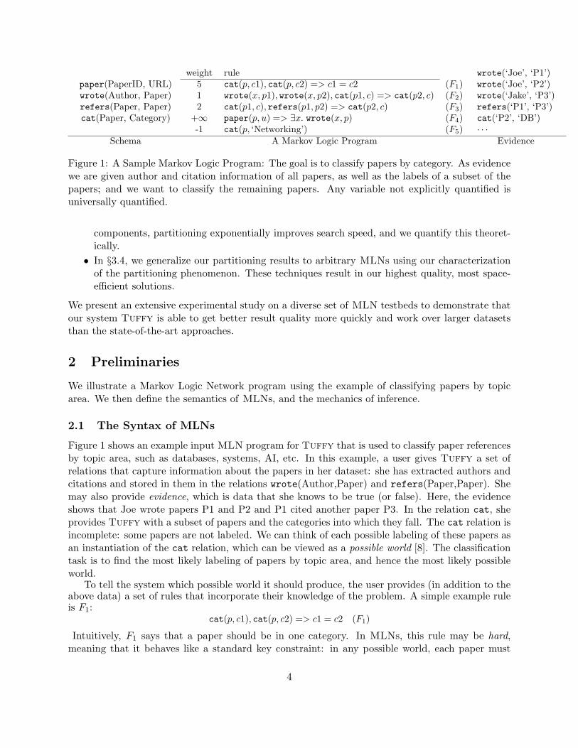
paper(PaperID, URL)wrote(Author, Paper)refers(Paper, Paper)cat(Paper, Category)

weight rule5 cat(p, c1), cat(p, c2) => c1 = c2 (F1)1 wrote(x, p1), wrote(x, p2), cat(p1, c) => cat(p2, c) (F2)2 cat(p1, c), refers(p1, p2) => cat(p2, c) (F3)

+∞ paper(p, u) => ∃x. wrote(x, p) (F4)-1 cat(p, ‘Networking’) (F5)

wrote(‘Joe’, ‘P1’)wrote(‘Joe’, ‘P2’)wrote(‘Jake’, ‘P3’)refers(‘P1’, ‘P3’)cat(‘P2’, ‘DB’)· · ·

Schema A Markov Logic Program Evidence

Figure 1: A Sample Markov Logic Program: The goal is to classify papers by category. As evidencewe are given author and citation information of all papers, as well as the labels of a subset of thepapers; and we want to classify the remaining papers. Any variable not explicitly quantified isuniversally quantified.

components, partitioning exponentially improves search speed, and we quantify this theoret-ically.• In §3.4, we generalize our partitioning results to arbitrary MLNs using our characterization

of the partitioning phenomenon. These techniques result in our highest quality, most space-efficient solutions.

We present an extensive experimental study on a diverse set of MLN testbeds to demonstrate thatour system Tuffy is able to get better result quality more quickly and work over larger datasetsthan the state-of-the-art approaches.

2 Preliminaries

We illustrate a Markov Logic Network program using the example of classifying papers by topicarea. We then define the semantics of MLNs, and the mechanics of inference.

2.1 The Syntax of MLNs

Figure 1 shows an example input MLN program for Tuffy that is used to classify paper referencesby topic area, such as databases, systems, AI, etc. In this example, a user gives Tuffy a set ofrelations that capture information about the papers in her dataset: she has extracted authors andcitations and stored in them in the relations wrote(Author,Paper) and refers(Paper,Paper). Shemay also provide evidence, which is data that she knows to be true (or false). Here, the evidenceshows that Joe wrote papers P1 and P2 and P1 cited another paper P3. In the relation cat, sheprovides Tuffy with a subset of papers and the categories into which they fall. The cat relation isincomplete: some papers are not labeled. We can think of each possible labeling of these papers asan instantiation of the cat relation, which can be viewed as a possible world [8]. The classificationtask is to find the most likely labeling of papers by topic area, and hence the most likely possibleworld.

To tell the system which possible world it should produce, the user provides (in addition to theabove data) a set of rules that incorporate their knowledge of the problem. A simple example ruleis F1:

cat(p, c1), cat(p, c2) => c1 = c2 (F1)

Intuitively, F1 says that a paper should be in one category. In MLNs, this rule may be hard,meaning that it behaves like a standard key constraint: in any possible world, each paper must

4

be in at most one category. This rule may also be soft, meaning that it may be violated in somepossible worlds. For example, in some worlds a paper may be in two categories. Soft rules also haveweights that intuitively tell us how likely the rule is to hold in a possible world. In this example, F1

is a soft rule and has weight 5. Roughly, this means that a fixed paper is e5 times more likely to bein a single category compared to being in 2 categories.2 MLNs can also involve data in non-trivialways, we refer the reader to §A.1 for a more complete exposition.

Query Model Given the data and the rules, a user may write arbitrary queries in terms of therelations. In Tuffy, the system is responsible for filling in whatever missing data is needed: in thisexample, the category of each unlabeled paper is unknown, and so to answer a query the systeminfers the most likely labels for each paper from the evidence.

2.2 Semantics of MLNs

We describe the semantics of MLNs. Formally, we first fix a schema σ (as in Figure 1) and a domainof constants D. Given as input a set of formula F = F1, . . . , FN (in clausal form3) with weightsw1, . . . , wN , they define a probability distribution over possible worlds (deterministic databases).To construct this probability distribution, the first step is grounding: given a formula F with freevariables x = (x1, . . . , xm), then for each d ∈ Dm, we create a new formula gd called a ground clausewhere gd denotes the result of substituting each variable xi of F with di. For example, for F3 thevariables are p1, p2, c: one tuple of constants is d = (‘P1’, ‘P2’, ‘DB’) and the ground formula fdis:

cat(‘P1’, ‘DB’), refers(‘P1’, ‘P2’) => cat(‘P2’, ‘DB’)

Each constituent in the ground formula, such as cat(‘P1’, ‘DB’) and refers(‘P1’, ‘P2’), is called aground predicate or atom for short. In the worst case there are D3 ground clauses for F3. For eachformula Fi (for i = 1 . . . N), we perform the above process. Each ground clause g of a formula Fi

is assigned the same weight, wi. So, a ground clause of F1 has weight 5, while any ground clauseof F2 has weight 1. We denote by G = (g, w) the set of all ground clauses of F and a function wthat maps each ground clause to its assigned weight. Fix an MLN F , then for any possible world(instance) I we say a ground clause g is violated if w(g) > 0 and g is false in I or if w(g) < 0 andg is true in I. We denote the set of ground clauses violated in a world I as V (I). The cost of theworld I is

cost(I) =∑

g∈V (I)

|w(g)| (1)

Through cost, an MLN defines a probability distribution over all instances (denoted Inst) as:

Pr[I] = Z−1 exp −cost(I) where Z =∑

J∈Inst

exp −cost(J)

A lowest cost world I is called a most likely world. Since cost(I) ≥ 0, if cost(I) = 0 then I is amost likely world. On the other hand the most likely world may have positive cost. There are twomain types of inference with MLNs: MAP inference, where we want to find a most likely world,

2In MLNs, it is not possible to give a direct probabilistic interpretation of weights [21]. In practice, the weightsassociated to formula are learned,which compensates for their non-intuitive nature. In this work, we do not discussthe mechanics of learning.

3Clausal form is a disjunction of positive or negative literals. For example, the rule is R(a) => R(b) is not inclausal form, but is equivalent to ¬R(a) ∨R(b), which is in clausal form.

5

and marginal inference, where we want to compute marginal probabilities. Tuffy is capable ofboth types of inference, but we present only MAP inference in the body of this paper. We referthe reader to §A.5 for details of marginal inference.

2.3 Inference

We now describe the state of the art of inference for MLNs (as in Alchemy, the reference MLNimplementation).

Grounding Conceptually, to obtain the ground clauses of an MLN formula F , the most straight-forward way is to enumerate all possible assignments to the free variables in F . There have beenseveral heuristics in the literature that improve the grounding process by pruning groundings thathave no effect on inference results; we describe the heuristics that Tuffy (and Alchemy) im-plements in §A.3. The set of ground clauses corresponds to a hypergraph where each atom is anode and each clause is a hyperedge. This graph structure is often called a Markov Random Field(MRF). We describe this structure formally in §A.2.

Search Finding a most likely world of an MLN is a generalization of the (NP-hard) MaxSATproblem. In this paper we concentrate on one of the most popular heuristic search algorithms,WalkSAT [14], which is used by Alchemy. WalkSAT works by repeatedly selecting a randomviolated clause and “fixing” it by flipping (i.e., changing the truth value of) an atom in it (see§A.4). As with any heuristic search, we cannot be sure that we have achieved the optimal, and sothe goal of any system that executes such a search procedure is: execute more search steps in thesame amount of time. To keep the comparison with Alchemy fair, we only discuss WalkSAT inthe body and defer our experience with other search algorithms to §C.1.

Problem Description The primary challenge that we address in this paper is scaling bothphases of MAP inference algorithms, grounding and search, using an RDBMS. Second, our goalis to improve the number of (effective) steps of the local search procedure using parallelism andpartitioning – but only when it provably improves the search quality. To achieve these goals,we attack three main technical challenges: (1) efficiently grounding large MLNs, (2) efficientlyperforming inference (search) on large MLNs, and (3) designing partitioning and partition-awaresearch algorithms that preserve (or enhance) search quality and speed.

3 Tuffy Systems

In this section, we describe our technical contributions: a bottom-up grounding approach to fullyleverage the RDBMS (§3.1); a hybrid main-memory RDBMS architecture to support efficient end-to-end inference (§3.2). In §3.3 and §3.4 we discuss data partitioning which dramatically improvesTuffy’s space and time efficiency.

3.1 Grounding with a Bottom-up Approach

We describe how Tuffy performs grounding. In contrast to top-down approaches (similar toProlog) that employ nested loops, Tuffy takes a bottom-up approach (similar to Datalog) and

6

expresses grounding as a sequence of SQL queries. Each SQL query is optimized by the RDBMS,which allows Tuffy to complete the grounding process orders of magnitude more quickly thanprior approaches.

For each predicate P (A) in the input MLN, Tuffy creates a relation RP (aid, A, truth) whereeach row ap represents an atom, aid is a globally unique identifier, A is the tuple of arguments ofP , and truth is a three-valued attribute that indicates if ap is true or false (in the evidence), or notspecified in the evidence. These tables form the input to grounding, and Tuffy constructs themusing standard bulk-loading techniques.

In Tuffy, we produce an output table C(cid, lits, weight) where each row corresponds to asingle ground clause. Here, cid is the id of a ground clause, lits is an array that stores the atomid of each literal in this clause (and whether or not it is negated), and weight is the weight ofthis clause. We first consider a formula without existential quantifiers. In this case, the formulaF can be written as F (x) = l1 ∨ · · · ∨ lN where x are all variables in F . Tuffy produces a SQLquery Q for F that joins together the relations corresponding to the predicates in F to producethe atom ids of the ground clauses (and whether or not they are negated). The join conditions inQ enforce variable equality inside F , and incorporate the pruning strategies described in §A.3. Formore details on the compilation procedure see §B.2.

3.2 A Hybrid Architecture for Inference

Our initial prototype of Tuffy ran both grounding and search in the RDBMS. While the groundingphase described in the previous section had good performance and scalability, we found that searchin an RDBMS is often a bottleneck. Thus, we design a hybrid architecture that allows efficientin-memory search while retaining the performance benefits of RDBMS-based grounding. To seewhy in-memory search is critical, recall that WalkSAT works by selecting an unsatisfied clause C,selecting an atom in C and “flipping” that atom to satisfy C. Thus, WalkSAT performs a largenumber of random accesses to the data representing ground clauses and atoms. Moreover, the datathat is accessed in one iteration depends on the data that is accessed in the previous iteration. Andso, this access pattern prevents both effective caching and parallelism, which causes a high overheadper data access. Thus, we implement a hybrid architecture where the RDBMS performs groundingand Tuffy is able to read the result of grounding from the RDBMS into memory and performinference. If the grounding result is too large to fit in memory, Tuffy invokes an implementationof search directly inside the RDBMS (§B.3). This approach is much less efficient than in-memorysearch, but it runs on very large datasets without crashing. §B.4 illustrates the architecture ofTuffy in more detail.

While it is clear that this hybrid approach is at least as scalable as a direct memory imple-mentation, such as Alchemy; in fact, there are cases where Tuffy can run in-memory searchwhile Alchemy would crash. The reason is that the space requirement of a purely in-memoryimplementation is determined by the peak memory footprint throughout grounding and search,whereas Tuffy needs main memory only for search. For example, on a dataset called RelationalClassification (RC), Alchemy allocated 2.8 GB of RAM only to produce 4.8 MB of ground clauses.On RC, Tuffy uses only 19 MB of RAM.

7

3.3 Partitioning to Improve Performance

In the following two sections, we study how to further improve Tuffy’s space and time efficiencywithout sacrificing its scalability. The underlying idea is simple: we will try to partition the data.By splitting the problem into smaller pieces, we can reduce the memory footprint and introduceparallelism, which conceptually breaks the sequential nature of the search. These are expectedbenefits of partitioning. An unexpected benefit is an exponentially increase of the effective searchspeed, a point that we return to below.

First, observe that the logical forms of MLNs often result in an MRF with multiple disjointcomponents (see §B.5). For example, on the RC dataset there are 489 components. Let G bean MRF with components G1, · · · , Gk; let I be a truth assignment to the atoms in G and Ii itsprojection over Gi. Then, it’s clear that ∀I:

costG(I) =∑

1≤i≤k

costGi(Ii).

Hence, instead of minimizing costG(I) directly, it suffices to minimize each individual costGi(Ii).The benefit is that, even if G itself does not fit in memory, it is possible that each Gi does. As such,we can solve each Gi with in-memory search one by one, and finally merge the results together.

Component detection is done after the grounding phase and before the search phase, as follows.We maintain an in-memory union-find structure over the nodes, and scan the clause table whileupdating the union-find structure. The end result is the set of connected components in the MRF.An immediate issue raised by partitioning is I/O efficiency.

Efficient Data Loading Once an MRF is split into components, loading in and running inferenceon each component sequentially one by one may incur many I/O operations, as there may be manypartitions. For example, the MRF of the Information Extraction (IE) dataset contains thousandsof 2-cliques and 3-cliques. One solution is to group the components into batches. The goal is tominimize the total number of batches (and thereby the I/O cost of loading), and the constraint isthat each batch cannot exceed the memory budget. This is essentially the bin packing problem,and we implement the First Fit Decreasing algorithm [28].

Once the partitions are in memory, we can take advantage of parallelism. In Tuffy, we executethreads using a round-robin policy. It is future work to consider more advanced thread schedulingpolicies, such as the Gittins Index in the multi-armed bandit literature [10].

Quality Although processing each component individually produces solutions that are no worsethan processing the whole graph at once, we give an example to illustrate that independentlyprocessing each component may result in exponentially faster speed of search.

Example 1 Consider an MRF consisting of N identical connected components each containingtwo atoms Xi, Yi and three weighted clauses

(Xi, 1), (Yi, 1), (Xi ∨ Yi,−1),

where i = 1 . . . N . Based on how WalkSAT works, it’s not hard to show that, if N = 1, startingfrom a random state, the expected hitting time4 of the optimal state, i.e. (X1, Y1) = (1, 1), is no

4The hitting time is a standard notion from Markov Chains [9], it is a random variable that represents the numberof steps taken by WalkSAT to reach an optimum for the first time.

8

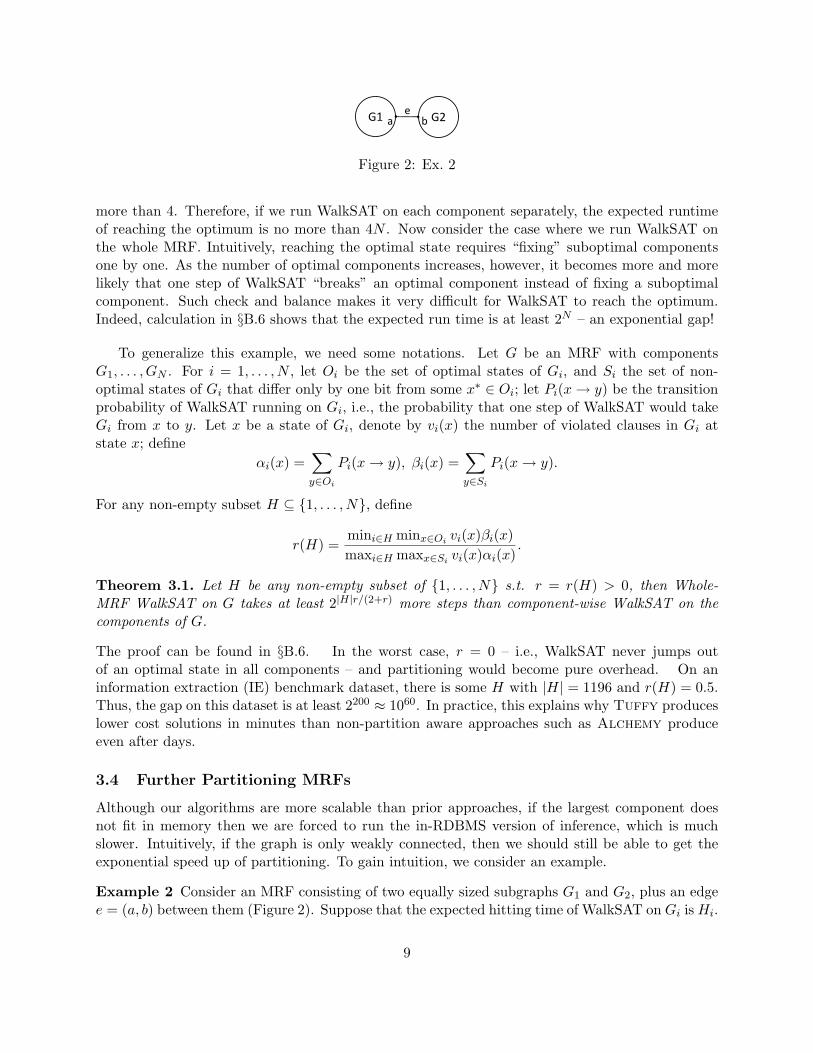
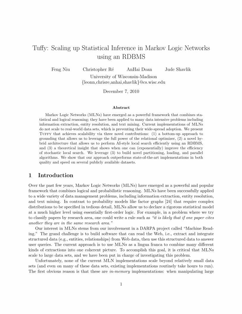
G1 G2 e

a b

Figure 2: Ex. 2

more than 4. Therefore, if we run WalkSAT on each component separately, the expected runtimeof reaching the optimum is no more than 4N . Now consider the case where we run WalkSAT onthe whole MRF. Intuitively, reaching the optimal state requires “fixing” suboptimal componentsone by one. As the number of optimal components increases, however, it becomes more and morelikely that one step of WalkSAT “breaks” an optimal component instead of fixing a suboptimalcomponent. Such check and balance makes it very difficult for WalkSAT to reach the optimum.Indeed, calculation in §B.6 shows that the expected run time is at least 2N – an exponential gap!

To generalize this example, we need some notations. Let G be an MRF with componentsG1, . . . , GN . For i = 1, . . . , N , let Oi be the set of optimal states of Gi, and Si the set of non-optimal states of Gi that differ only by one bit from some x∗ ∈ Oi; let Pi(x→ y) be the transitionprobability of WalkSAT running on Gi, i.e., the probability that one step of WalkSAT would takeGi from x to y. Let x be a state of Gi, denote by vi(x) the number of violated clauses in Gi atstate x; define

αi(x) =∑y∈Oi

Pi(x→ y), βi(x) =∑y∈Si

Pi(x→ y).

For any non-empty subset H ⊆ 1, . . . , N, define

r(H) =mini∈H minx∈Oi vi(x)βi(x)maxi∈H maxx∈Si vi(x)αi(x)

.

Theorem 3.1. Let H be any non-empty subset of 1, . . . , N s.t. r = r(H) > 0, then Whole-MRF WalkSAT on G takes at least 2|H|r/(2+r) more steps than component-wise WalkSAT on thecomponents of G.

The proof can be found in §B.6. In the worst case, r = 0 – i.e., WalkSAT never jumps outof an optimal state in all components – and partitioning would become pure overhead. On aninformation extraction (IE) benchmark dataset, there is some H with |H| = 1196 and r(H) = 0.5.Thus, the gap on this dataset is at least 2200 ≈ 1060. In practice, this explains why Tuffy produceslower cost solutions in minutes than non-partition aware approaches such as Alchemy produceeven after days.

3.4 Further Partitioning MRFs

Although our algorithms are more scalable than prior approaches, if the largest component doesnot fit in memory then we are forced to run the in-RDBMS version of inference, which is muchslower. Intuitively, if the graph is only weakly connected, then we should still be able to get theexponential speed up of partitioning. To gain intuition, we consider an example.

Example 2 Consider an MRF consisting of two equally sized subgraphs G1 and G2, plus an edgee = (a, b) between them (Figure 2). Suppose that the expected hitting time of WalkSAT on Gi is Hi.

9

Since H1 and H2 are essentially independent, the hitting time of WalkSAT on G could be roughlyH1H2. On the other hand, consider the following scheme: enumerate all possible truth assignmentsto one of the boundary variables a, b, say a – of which there are two – and conditioning on eachassignment, run WalkSAT on G1 and G2 independently. Clearly, the overall hitting time is nomore than 2(H1 + H2), which is a huge improvement over H1H2 since Hi is usually a high-orderpolynomial or even exponential in the size of Gi.

To capitalize on this idea, we need to address two challenges: 1) designing an efficient MRFpartitioning algorithm; and 2) designing an effective partition-aware search algorithm. We addresseach of them in turn.

MRF Partitioning Intuitively, to maximally utilize the memory budget, we want to partitionthe MRF into roughly equal sizes; to minimize information loss, we want to minimize total weightof clauses that span over multiple partitions, i.e., the cut size. To capture this notion, we define abalanced bisection of a hypergraph G = (V,E) as a partition of V = V1 ∪ V2 such that |V1| = |V2|.The cost of a bisection (V1, V2) is |e ∈ E|e ∩ V1 6= ∅ and e ∩ V2 6= ∅|.

Theorem 3.2. Consider the MLN Γ given by the single rule p(x), r(x, y) → p(y) where r is anevidence predicate. Then, the problem of finding a minimum-cost balanced bisection of the MRFthat results from Γ is NP-hard in the size of the evidence (data).

The proof (§B.7) is by reduction to the graph minimum bisection problem [15], which is hardto approximate (unless P = NP, there is no PTAS). In fact, the problem we are facing (multi-way hypergraph partitioning) is more challenging than graph bisection, and has been extensivelystudied [13, 25]. And so, we design a simple, greedy partitioning algorithm: it assigns each clauseto a bin in descending order by clause weight, subject to the constraint that no component in theresulting graph is larger than an input parameter β. We include pseudocode in §B.8.

Partition-aware Search We need to refine the search procedure to be aware of partitions: thecentral challenge is that a clause in the cut may depend on atoms in two distinct partitions. Hence,there are dependencies between the partitions. We exploit the idea in Example 2 to design thefollowing partition-aware search scheme – which is an instance of the Gauss-Seidel method fromnonlinear optimization [3, pg. 219]. Denote by X1, . . . , Xk the states (i.e., truth assignments to theatoms) of the partitions. First initialize Xi = x0

i for i = 1 . . . k. For t = 1 . . . T , for i = 1 . . . k, runWalkSAT on xt−1

i conditioned on xtj |1 ≤ j < i ∪ xt−1

j |i < j ≤ k to obtain xti. Finally, return

xTi |1 ≤ i ≤ k.

4 Experiments

In this section, we validate first that our system Tuffy is orders of magnitude more scalable andefficient than prior approaches. We then validate that each of our techniques contributes to thegoal.

Experimental Setup We select Alchemy, the currently most widely used MLN system, as ourcomparison point. Alchemy and Tuffy are implemented in C++ and Java, respectively. TheRDBMS used by Tuffy is PostgreSQL 8.4. Unless specified otherwise, all experiments are run

10

on an Intel Core2 at 2.4GHz with 4 GB of RAM running Red Hat Enterprise Linux 5. For faircomparison, in all experiments Tuffy runs a single thread unless otherwise noted.

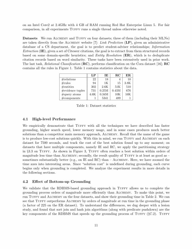
Datasets We run Alchemy and Tuffy on four datasets; three of them (including their MLNs)are taken directly from the Alchemy website [7]: Link Prediction (LP), given an administrativedatabase of a CS department, the goal is to predict student-adviser relationships; InformationExtraction (IE), given a set of Citeseer citations, the goal is to extract from them structured recordsbased on some domain-specific heuristics; and Entity Resolution (ER), which is to deduplicatecitation records based on word similarity. These tasks have been extensively used in prior work.The last task, Relational Classification (RC), performs classification on the Cora dataset [16]; RCcontains all the rules in Figure 1. Table 1 contains statistics about the data.

LP IE RC ER#relations 22 18 4 10#rules 94 1K 15 3.8K#entities 302 2.6K 51K 510#evidence tuples 731 0.25M 0.43M 676#query atoms 4.6K 0.34M 10K 16K#components 1 5341 489 1

Table 1: Dataset statistics

4.1 High-level Performance

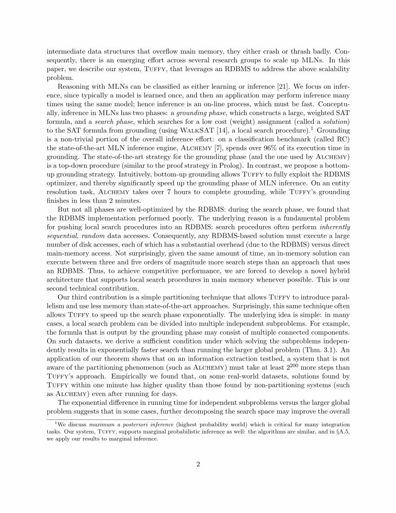
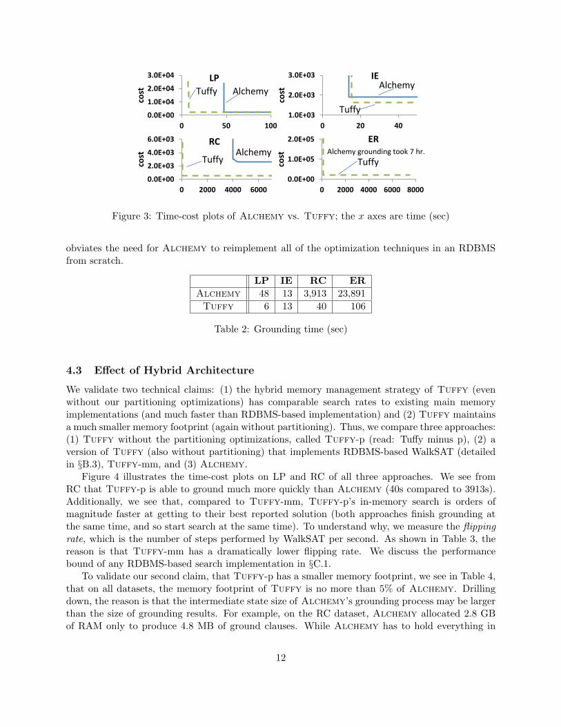
We empirically demonstrate that Tuffy with all the techniques we have described has fastergrounding, higher search speed, lower memory usage, and in some cases produces much bettersolutions than a competitor main memory approach, Alchemy. Recall that the name of the gameis to produce low-cost solutions quickly. With this in mind, we run Tuffy and Alchemy on eachdataset for 7500 seconds, and track the cost of the best solution found up to any moment; ondatasets that have multiple components, namely IE and RC, we apply the partitioning strategyin §3.3 on Tuffy. As shown in Figure 3, Tuffy often reaches a best solution within orders ofmagnitude less time than Alchemy; secondly, the result quality of Tuffy is at least as good as –sometimes substantially better (e.g., on IE and RC) than – Alchemy. Here, we have zoomed thetime axes into interesting areas. Since “solution cost” is undefined during grounding, each curvebegins only when grounding is completed. We analyze the experiment results in more details inthe following sections.

4.2 Effect of Bottom-up Grounding

We validate that the RDBMS-based grounding approach in Tuffy allows us to complete thegrounding process orders of magnitude more efficiently than Alchemy. To make this point, werun Tuffy and Alchemy on the four datasets, and show their grounding time in Table 2. We cansee that Tuffy outperforms Alchemy by orders of magnitude at run time in the grounding phase(a factor of 225 on the ER dataset). To understand the differences, we dug deeper with a lesionstudy, and found that sort join and hash join algorithms (along with predicate pushdown) are thekey components of the RDBMS that speeds up the grounding process of Tuffy (§C.2). Tuffy

11

1.0E+03

2.0E+03

3.0E+03

0 20 40

cost

IE Alchemy

Tuffy 0.0E+00

1.0E+04

2.0E+04

3.0E+04

0 50 100

cost

LP

Alchemy Tuffy

0.0E+00

1.0E+05

2.0E+05

0 2000 4000 6000 8000

cost

ER Alchemy grounding took 7 hr.

Tuffy

0.0E+00

2.0E+03

4.0E+03

6.0E+03

0 2000 4000 6000

cost

RC

Alchemy Tuffy

Figure 3: Time-cost plots of Alchemy vs. Tuffy; the x axes are time (sec)

obviates the need for Alchemy to reimplement all of the optimization techniques in an RDBMSfrom scratch.

LP IE RC ERAlchemy 48 13 3,913 23,891Tuffy 6 13 40 106

Table 2: Grounding time (sec)

4.3 Effect of Hybrid Architecture

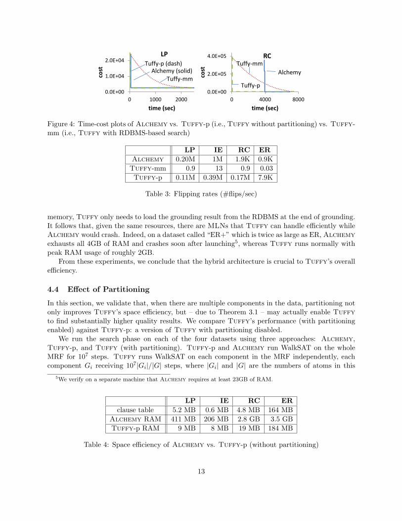
We validate two technical claims: (1) the hybrid memory management strategy of Tuffy (evenwithout our partitioning optimizations) has comparable search rates to existing main memoryimplementations (and much faster than RDBMS-based implementation) and (2) Tuffy maintainsa much smaller memory footprint (again without partitioning). Thus, we compare three approaches:(1) Tuffy without the partitioning optimizations, called Tuffy-p (read: Tuffy minus p), (2) aversion of Tuffy (also without partitioning) that implements RDBMS-based WalkSAT (detailedin §B.3), Tuffy-mm, and (3) Alchemy.

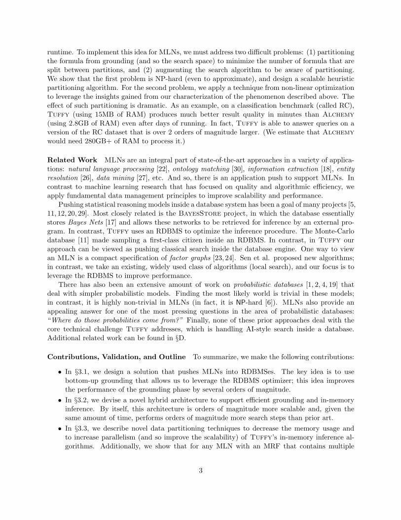
Figure 4 illustrates the time-cost plots on LP and RC of all three approaches. We see fromRC that Tuffy-p is able to ground much more quickly than Alchemy (40s compared to 3913s).Additionally, we see that, compared to Tuffy-mm, Tuffy-p’s in-memory search is orders ofmagnitude faster at getting to their best reported solution (both approaches finish grounding atthe same time, and so start search at the same time). To understand why, we measure the flippingrate, which is the number of steps performed by WalkSAT per second. As shown in Table 3, thereason is that Tuffy-mm has a dramatically lower flipping rate. We discuss the performancebound of any RDBMS-based search implementation in §C.1.

To validate our second claim, that Tuffy-p has a smaller memory footprint, we see in Table 4,that on all datasets, the memory footprint of Tuffy is no more than 5% of Alchemy. Drillingdown, the reason is that the intermediate state size of Alchemy’s grounding process may be largerthan the size of grounding results. For example, on the RC dataset, Alchemy allocated 2.8 GBof RAM only to produce 4.8 MB of ground clauses. While Alchemy has to hold everything in

12

0.0E+00

1.0E+04

2.0E+04

0 1000 2000co

st

time (sec)

LP

Alchemy (solid) Tuffy-p (dash)

Tuffy-mm

0.0E+00

2.0E+05

4.0E+05

0 4000 8000

cost

time (sec)

RC

Alchemy

Tuffy-p

Tuffy-mm

Figure 4: Time-cost plots of Alchemy vs. Tuffy-p (i.e., Tuffy without partitioning) vs. Tuffy-mm (i.e., Tuffy with RDBMS-based search)

LP IE RC ERAlchemy 0.20M 1M 1.9K 0.9KTuffy-mm 0.9 13 0.9 0.03Tuffy-p 0.11M 0.39M 0.17M 7.9K

Table 3: Flipping rates (#flips/sec)

memory, Tuffy only needs to load the grounding result from the RDBMS at the end of grounding.It follows that, given the same resources, there are MLNs that Tuffy can handle efficiently whileAlchemy would crash. Indeed, on a dataset called “ER+” which is twice as large as ER, Alchemyexhausts all 4GB of RAM and crashes soon after launching5, whereas Tuffy runs normally withpeak RAM usage of roughly 2GB.

From these experiments, we conclude that the hybrid architecture is crucial to Tuffy’s overallefficiency.

4.4 Effect of Partitioning

In this section, we validate that, when there are multiple components in the data, partitioning notonly improves Tuffy’s space efficiency, but – due to Theorem 3.1 – may actually enable Tuffyto find substantially higher quality results. We compare Tuffy’s performance (with partitioningenabled) against Tuffy-p: a version of Tuffy with partitioning disabled.

We run the search phase on each of the four datasets using three approaches: Alchemy,Tuffy-p, and Tuffy (with partitioning). Tuffy-p and Alchemy run WalkSAT on the wholeMRF for 107 steps. Tuffy runs WalkSAT on each component in the MRF independently, eachcomponent Gi receiving 107|Gi|/|G| steps, where |Gi| and |G| are the numbers of atoms in this

5We verify on a separate machine that Alchemy requires at least 23GB of RAM.

LP IE RC ERclause table 5.2 MB 0.6 MB 4.8 MB 164 MB

Alchemy RAM 411 MB 206 MB 2.8 GB 3.5 GBTuffy-p RAM 9 MB 8 MB 19 MB 184 MB

Table 4: Space efficiency of Alchemy vs. Tuffy-p (without partitioning)

13

component and the MRF, respectively. This is weighted round-robin scheduling.

LP IE RC ER#components 1 5341 489 1Tuffy-p RAM 9MB 8MB 19MB 184MBTuffy RAM 9MB 8MB 15MB 184MBTuffy-p cost 2534 1933 1943 18717Tuffy cost 2534 1635 1281 18717

Table 5: Performance of Tuffy vs. Tuffy-p (i.e., Tuffy without partitioning)

1000

1400

1800

2200

2600

0 20 40 60 80

cost

time (sec)

IE

Tuffy

Tuffy-p (dotted) Alchemy (solid)

0

1000

2000

3000

0 100 200 300co

st

time (sec)

RC

Tuffy

Tuffy-p

Alchemy grounding took over 1 hr.

Figure 5: Time-cost plots of Tuffy vs Tuffy-p (i.e., Tuffy without partitioning)

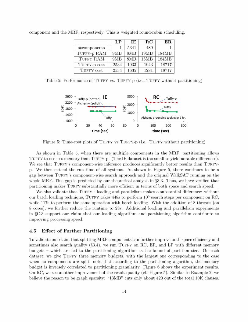
As shown in Table 5, when there are multiple components in the MRF, partitioning allowsTuffy to use less memory than Tuffy-p. (The IE dataset is too small to yield notable differences).We see that Tuffy’s component-wise inference produces significantly better results than Tuffy-p. We then extend the run time of all systems. As shown in Figure 5, there continues to be agap between Tuffy’s component-wise search approach and the original WalkSAT running on thewhole MRF. This gap is predicted by our theoretical analysis in §3.3. Thus, we have verified thatpartitioning makes Tuffy substantially more efficient in terms of both space and search speed.

We also validate that Tuffy’s loading and parallelism makes a substantial difference: withoutour batch loading technique, Tuffy takes 448s to perform 106 search steps per component on RC,while 117s to perform the same operation with batch loading. With the addition of 8 threads (on8 cores), we further reduce the runtime to 28s. Additional loading and parallelism experimentsin §C.3 support our claim that our loading algorithm and partitioning algorithm contribute toimproving processing speed.

4.5 Effect of Further Partitioning

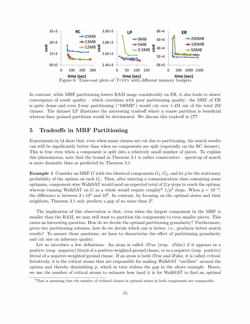
To validate our claim that splitting MRF components can further improve both space efficiency andsometimes also search quality (§3.4), we run Tuffy on RC, ER, and LP with different memorybudgets – which are fed to the partitioning algorithm as the bound of partition size. On eachdataset, we give Tuffy three memory budgets, with the largest one corresponding to the casewhen no components are split; note that according to the partitioning algorithm, the memorybudget is inversely correlated to partitioning granularity. Figure 6 shows the experiment results.On RC, we see another improvement of the result quality (cf. Figure 5). Similar to Example 2, webelieve the reason to be graph sparsity: “13MB” cuts only about 420 out of the total 10K clauses.

14

0E+0

1E+3

2E+3

3E+3

0 100 200 300

cost

time (sec)

RC 15MB13MB12MB

2.4E+3

2.6E+3

2.8E+3

3.0E+3

0 50 100 150

cost

time (sec)

LP

9MB5MB3.5MB

0E+0

2E+4

4E+4

6E+4

8E+4

0 500 1000 1500

cost

time (sec)

ER 200MB

100MB

50MB

Figure 6: Time-cost plots of Tuffy with different memory budgets

In contrast, while MRF partitioning lowers RAM usage considerably on ER, it also leads to slowerconvergence of result quality – which correlates with poor partitioning quality: the MRF of ERis quite dense and even 2-way partitioning (“100MB”) would cut over 1.4M out of the total 2Mclauses. The dataset LP illustrates the interesting tradeoff where a coarse partition is beneficialwhereas finer grained partitions would be detrimental. We discuss this tradeoff in §??.

5 Tradeoffs in MRF Partitioning

Experiments in §4 show that, even when many clauses are cut due to partitioning, the search resultscan still be significantly better than when no components are split (especially on the RC dataset).This is true even when a component is split into a relatively small number of pieces. To explainthis phenomenon, note that the bound in Theorem 3.1 is rather conservative – speed-up of searchis more dramatic than as predicted by Theorem 3.1.

Example 1 Consider an MRF G with two identical components G1, G2, and let p be the stationaryprobability of the optima on each Gi. Then, after entering a communication class containing someoptimum, component-wise WalkSAT would need an expected total of 2/p steps to reach the optima;whereas running WalkSAT on G as a whole would require roughly6 1/p2 steps. When p = 10−4,the difference is between 2 ∗ 104 and 108. In contrast, by focusing on the optimal states and theirneighbors, Theorem 3.1 only predicts a gap of no more than 22.

The implication of this observation is that, even when the largest component in the MRF issmaller than the RAM, we may still want to partition the components to even smaller pieces. Thisraises an interesting question: How do we decide the optimal partitioning granularity? Furthermore,given two partitioning schemes, how do we decide which one is better, i.e., produces better searchresults? To answer those questions, we have to characterize the effect of partitioning granularityand cut size on inference quality.

Let us introduce a few definitions. An atom is called iTrue (resp. iFalse) if it appears in apositive (resp. negative) literal of a positive-weighted ground clause, or in a negative (resp. positive)literal of a negative-weighted ground clause. If an atom is both iTrue and iFalse, it is called critical.Intuitively, it is the critical atoms that are responsible for making WalkSAT “oscillate” around theoptima and thereby diminishing p, which in turn widens the gap in the above example. Hence,we use the number of critical atoms to estimate how hard it is for WalkSAT to find an optimal

6That is assuming that the number of violated clauses in optimal states in both components are comparable.

15

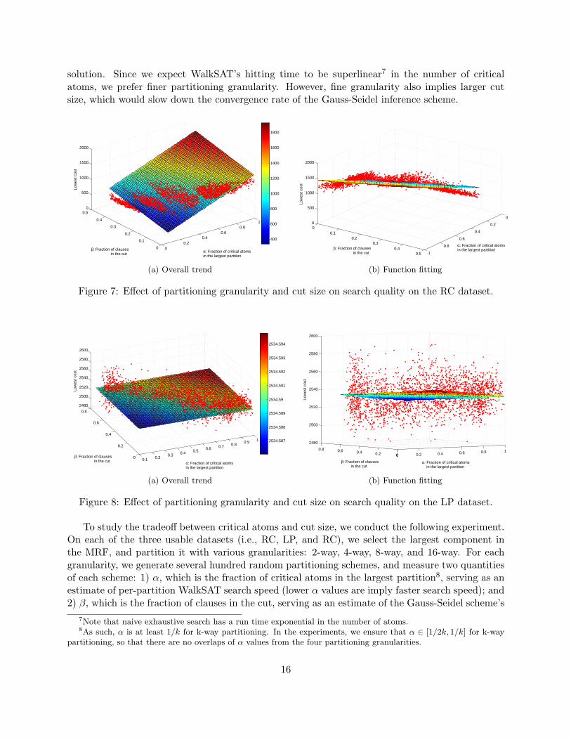
solution. Since we expect WalkSAT’s hitting time to be superlinear7 in the number of criticalatoms, we prefer finer partitioning granularity. However, fine granularity also implies larger cutsize, which would slow down the convergence rate of the Gauss-Seidel inference scheme.

00.2

0.40.6

0.81

0

0.1

0.2

0.3

0.4

0.50

500

1000

1500

2000

α: Fraction of critical atomsin the largest partition

β: Fraction of clausesin the cut

Low

est c

ost

400

600

800

1000

1200

1400

1600

1800

(a) Overall trend

0

0.2

0.4

0.6

0.8

1

00.1

0.20.3

0.40.5

0

500

1000

1500

2000

α: Fraction of critical atomsin the largest partitionβ: Fraction of clauses

in the cut

Low

est c

ost

(b) Function fitting

Figure 7: Effect of partitioning granularity and cut size on search quality on the RC dataset.

0.1 0.20.3 0.4 0.5

0.6 0.7 0.80.9 1

0

0.2

0.4

0.6

0.8

2480

2500

2520

2540

2560

2580

2600

α: Fraction of critical atomsin the largest partition

β: Fraction of clausesin the cut

Low

est c

ost

2534.587

2534.588

2534.589

2534.59

2534.591

2534.592

2534.593

2534.594

(a) Overall trend

0 0.2 0.4 0.6 0.8 100.20.40.60.8

2480

2500

2520

2540

2560

2580

2600

α: Fraction of critical atomsin the largest partition

β: Fraction of clausesin the cut

Low

est c

ost

(b) Function fitting

Figure 8: Effect of partitioning granularity and cut size on search quality on the LP dataset.

To study the tradeoff between critical atoms and cut size, we conduct the following experiment.On each of the three usable datasets (i.e., RC, LP, and RC), we select the largest component inthe MRF, and partition it with various granularities: 2-way, 4-way, 8-way, and 16-way. For eachgranularity, we generate several hundred random partitioning schemes, and measure two quantitiesof each scheme: 1) α, which is the fraction of critical atoms in the largest partition8, serving as anestimate of per-partition WalkSAT search speed (lower α values are imply faster search speed); and2) β, which is the fraction of clauses in the cut, serving as an estimate of the Gauss-Seidel scheme’s

7Note that naive exhaustive search has a run time exponential in the number of atoms.8As such, α is at least 1/k for k-way partitioning. In the experiments, we ensure that α ∈ [1/2k, 1/k] for k-way

partitioning, so that there are no overlaps of α values from the four partitioning granularities.

16

00.2

0.40.6

0.81

0

0.2

0.4

0.6

0.8

11

1.5

2

2.5

3

3.5

4

x 104

α: Fraction of critical atomsin the largest partition

β: Fraction of clausesin the cut

Low

est c

ost

1.6

1.8

2

2.2

2.4

2.6

2.8

3

3.2

3.4

3.6x 10

4

(a) Overall trend

00.2

0.40.6

0.81

00.2

0.40.6

0.81

1

1.5

2

2.5

3

3.5

4

x 104

α: Fraction of critical atomsin the largest partition

β: Fraction of clausesin the cut

Low

est c

ost

(b) Function fitting

Figure 9: Effect of partitioning granularity and cut size on search quality on the ER dataset.

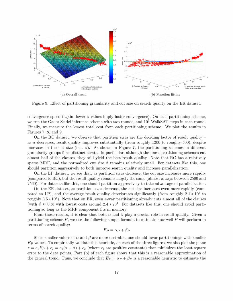
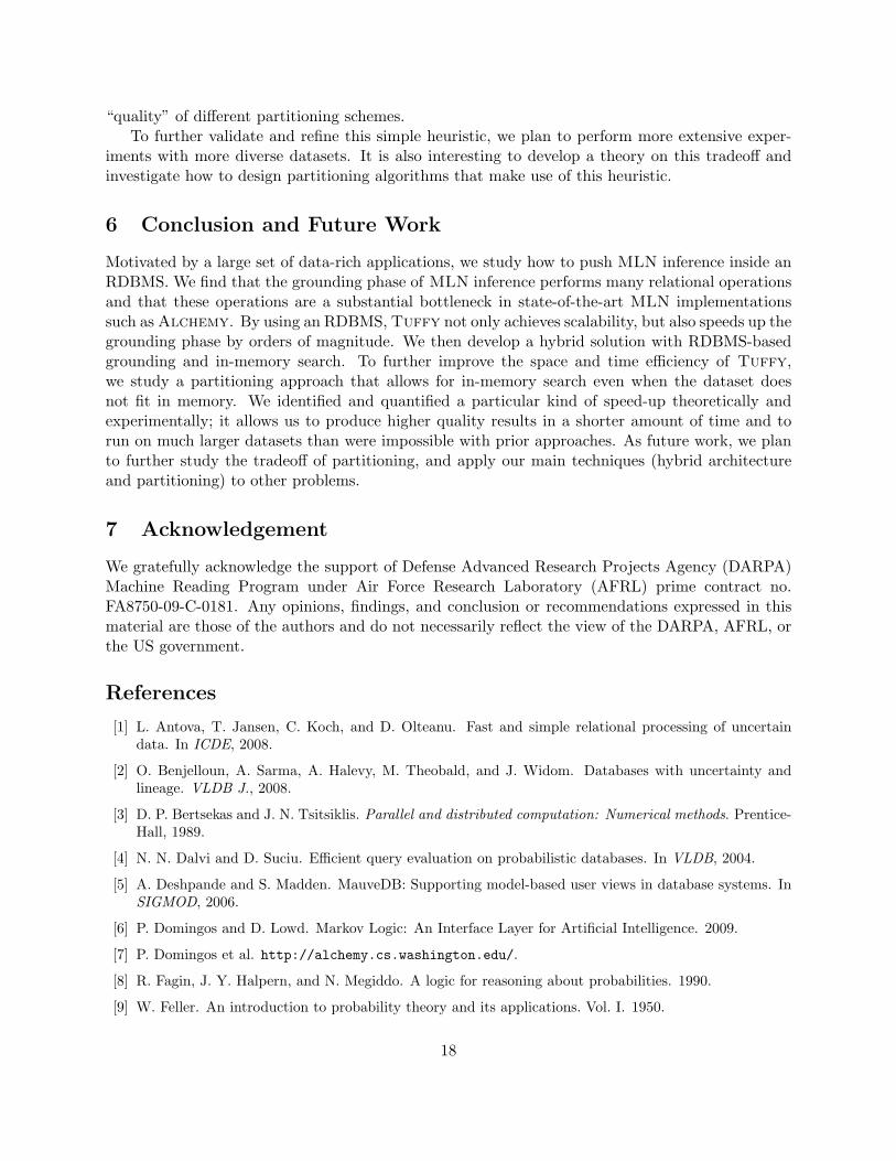
convergence speed (again, lower β values imply faster convergence). On each partitioning scheme,we run the Gauss-Seidel inference scheme with two rounds, and 105 WalkSAT steps in each round.Finally, we measure the lowest total cost from each partitioning scheme. We plot the results inFigures 7, 8, and 9.

On the RC dataset, we observe that partition sizes are the deciding factor of result quality –as α decreases, result quality improves substantially (from roughly 1200 to roughly 500), despiteincreases in the cut size (i.e., β). As shown in Figure 7, the partitioning schemes in differentgranularity groups form distinct strata. In particular, although the finest partitioning schemes cutalmost half of the clauses, they still yield the best result quality. Note that RC has a relativelysparse MRF, and the normalized cut size β remains relatively small. For datasets like this, oneshould partition aggressively to both improve search quality and increase parallelization.

On the LP dataset, we see that, as partition sizes decrease, the cut size increases more rapidly(compared to RC), but the result quality remains largely the same (almost always between 2500 and2560). For datasets like this, one should partition aggressively to take advantage of parallelization.

On the ER dataset, as partition sizes decrease, the cut size increases even more rapidly (com-pared to LP), and the average result quality deteriorates significantly (from roughly 2.1 ∗ 104 toroughly 3.5 ∗ 104). Note that on ER, even 4-way partitioning already cuts almost all of the clauses(with β ≈ 0.8) with lowest costs around 2.4 ∗ 204. For datasets like this, one should avoid parti-tioning so long as the MRF component fits in memory.

From those results, it is clear that both α and β play a crucial role in result quality. Given apartitioning scheme P , we use the following simple formula to estimate how well P will perform interms of search quality:

EP = αP + βP

Since smaller values of α and β are more desirable, one should favor partitionings with smallerEP values. To empirically validate this heuristic, on each of the three figures, we also plot the planez = c1EP + c2 = c1(α + β) + c2 (where ci are positive constants) that minimizes the least squareerror to the data points. Part (b) of each figure shows that this is a reasonable approximation ofthe general trend. Thus, we conclude that EP = αP + βP is a reasonable heuristic to estimate the

17

“quality” of different partitioning schemes.To further validate and refine this simple heuristic, we plan to perform more extensive exper-

iments with more diverse datasets. It is also interesting to develop a theory on this tradeoff andinvestigate how to design partitioning algorithms that make use of this heuristic.

6 Conclusion and Future Work

Motivated by a large set of data-rich applications, we study how to push MLN inference inside anRDBMS. We find that the grounding phase of MLN inference performs many relational operationsand that these operations are a substantial bottleneck in state-of-the-art MLN implementationssuch as Alchemy. By using an RDBMS, Tuffy not only achieves scalability, but also speeds up thegrounding phase by orders of magnitude. We then develop a hybrid solution with RDBMS-basedgrounding and in-memory search. To further improve the space and time efficiency of Tuffy,we study a partitioning approach that allows for in-memory search even when the dataset doesnot fit in memory. We identified and quantified a particular kind of speed-up theoretically andexperimentally; it allows us to produce higher quality results in a shorter amount of time and torun on much larger datasets than were impossible with prior approaches. As future work, we planto further study the tradeoff of partitioning, and apply our main techniques (hybrid architectureand partitioning) to other problems.

7 Acknowledgement

We gratefully acknowledge the support of Defense Advanced Research Projects Agency (DARPA)Machine Reading Program under Air Force Research Laboratory (AFRL) prime contract no.FA8750-09-C-0181. Any opinions, findings, and conclusion or recommendations expressed in thismaterial are those of the authors and do not necessarily reflect the view of the DARPA, AFRL, orthe US government.

References

[1] L. Antova, T. Jansen, C. Koch, and D. Olteanu. Fast and simple relational processing of uncertaindata. In ICDE, 2008.

[2] O. Benjelloun, A. Sarma, A. Halevy, M. Theobald, and J. Widom. Databases with uncertainty andlineage. VLDB J., 2008.

[3] D. P. Bertsekas and J. N. Tsitsiklis. Parallel and distributed computation: Numerical methods. Prentice-Hall, 1989.

[4] N. N. Dalvi and D. Suciu. Efficient query evaluation on probabilistic databases. In VLDB, 2004.

[5] A. Deshpande and S. Madden. MauveDB: Supporting model-based user views in database systems. InSIGMOD, 2006.

[6] P. Domingos and D. Lowd. Markov Logic: An Interface Layer for Artificial Intelligence. 2009.

[7] P. Domingos et al. http://alchemy.cs.washington.edu/.

[8] R. Fagin, J. Y. Halpern, and N. Megiddo. A logic for reasoning about probabilities. 1990.

[9] W. Feller. An introduction to probability theory and its applications. Vol. I. 1950.

18

[10] S. Guha and K. Munagala. Multi-armed bandits with metric switching costs. ICALP, 2009.

[11] R. Jampani, F. Xu, M. Wu, L. L. Perez, C. M. Jermaine, and P. J. Haas. MCDB: a monte carloapproach to managing uncertain data. In SIGMOD, 2008.

[12] B. Kanagal and A. Deshpande. Online filtering, smoothing and probabilistic modeling of streamingdata. In ICDE, 2008.

[13] G. Karypis, R. Aggarwal, V. Kumar, and S. Shekhar. Multilevel hypergraph partitioning: Applicationsin VLSI domain. VLSI Systems, IEEE Transactions on, 2002.

[14] H. Kautz, B. Selman, and Y. Jiang. A general stochastic approach to solving problems with hard andsoft constraints. The Satisfiability Problem: Theory and Applications, 1997.

[15] S. Khot. Ruling out PTAS for graph min-bisection, densest subgraph and bipartite clique. In FOCS,2004.

[16] A. McCallum, K. Nigam, J. Rennie, and K. Seymore. Automating the construction of internet portalswith machine learning. Information Retrieval Journal, 2000.

[17] J. Pearl. Probabilistic reasoning in intelligent systems: networks of plausible inference. 1988.

[18] H. Poon and P. Domingos. Joint inference in information extraction. In AAAI ’07.

[19] C. Re, N. N. Dalvi, and D. Suciu. Efficient top-k query evaluation on probabilistic data. In ICDE, 2007.

[20] C. Re, J. Letchner, M. Balazinska, and D. Suciu. Event queries on correlated probabilistic streams. InSIGMOD, 2008.

[21] M. Richardson and P. Domingos. Markov logic networks. Machine Learning, 2006.

[22] S. Riedel and I. Meza-Ruiz. Collective semantic role labeling with Markov logic. In CoNLL ’08.

[23] P. Sen and A. Deshpande. Representing and querying correlated tuples in probabilistic databases. InICDE, 2007.

[24] P. Sen, A. Deshpande, and L. Getoor. PrDB: managing and exploiting rich correlations in probabilisticdatabases. VLDB J., 2009.

[25] H. Simon and S. Teng. How good is recursive bisection? SIAM Journal on Scientific Computing, 1997.

[26] P. Singla and P. Domingos. Entity resolution with Markov logic. In ICDE ’06.

[27] P. Singla, H. Kautz, J. Luo, and A. Gallagher. Discovery of social relationships in consumer photocollections using Markov Logic. In CVPR Workshops 2008.

[28] V. Vazirani. Approximation algorithms. Springer Verlag, 2001.

[29] D. Z. Wang, E. Michelakis, M. N. Garofalakis, and J. M. Hellerstein. BayesStore: managing large,uncertain data repositories with probabilistic graphical models. PVLDB, 2008.

[30] F. Wu and D. S. Weld. Automatically refining the Wikipedia infobox ontology. In WWW ’08, 2008.

19

A Material for Preliminaries

A.1 More Details on the MLN Program

Rules in MLNs are expressive and may involve data in non-trivial ways. For example, consider F2:

wrote(x, p1), wrote(x, p2), cat(p1, c) => cat(p2, c) (F2)

Intuitively, this rule says that all the papers written by a particular person are likely to be in thesame category. Rules may also have existential quantifiers: F4 says “any paper in our databasemust have at least one author.” It is also a hard rule, which is indicated by the infinite weight, andso no possible world may violate this rule. The weight of a formula may also be negative, whicheffectively means that the negation of the formula is likely to hold. For example, F5 models ourbelief that none or very few of the unlabeled papers belong to ‘Networking’. Tuffy supports allof these features.

If the input MLN contains hard rules (indicated by a weight of +∞ or −∞), then we insistthat the set of possible worlds (Inst) only contain worlds that satisfy every hard rule with +∞ andviolate every rule with −∞. In practice, schemata have type information, and we can use this toremove nonsensical ground clauses, e.g., both attributes of refers are paper references, and so itis unnecessary to ground this predicate with another type, say person.

A.2 Markov Random Field

A Boolean Markov Random Field (or Boolean Markov network is a model of the joint distributionof a set of Boolean random variables X = (X1, . . . , XN ). It is defined by a hypergraph G = (X,E);for each hyperedge e ∈ E there is a potential function (aka “feature”) denoted φe, which is afunction from the values of the set of variables in e to non-negative real numbers. This defines ajoint distribution Pr(X = x) as follows:

Pr(X = x) =1Z

∏e∈E

φe(xe)

where x ∈ 0, 1N , Z is a normalization constant and xe denotes the values of the variables in e.Fix a set of constants C = c1, . . . , cM. An MLN defines a Boolean Markov Random Field as

follows: for each possible grounding of each predicate (i.e., atom), create a node (and so a Booleanrandom variable). For example, there will be a node refers(p1, p2) for each pair of papers p1, p2.For each formula Fi we ground it in all possible ways, then we create a hyperedge e that contains thenodes corresponding to all terms in the formula. For example, the key constraint creates hyperedgesfor each paper and all of its potential categories. We refer to this graph as the ground network.Once we have the ground network, our task reduces to inference in Markov models.

Explicitly representing such ground networks is prohibitively expensive and unnecessary. Inpractice, we only include non-evidence nodes and groundings that are relevant to answering thequery (see §A.3).

A.3 Optimizing MLN Grounding Process

Conceptually, we might ground an MLN formula by enumerating all possible assignments to itsfree variables. However, this is both impractical and unnecessary. For example, if we ground F2

20

exhaustively this way, the result would contain |D|4 ground clauses. Fortunately, in practice avast majority of ground clauses are satisfied by evidence regardless of the assignments to unknowntruth values; we can safely discard such clauses [42]. Consider the ground clause gd of F2 whered =(‘Joe’, ‘P2’, ‘P3’, ‘DB’). Suppose that wrote(‘Joe’, ‘P3’) is known to be false, then gd will besatisfied no matter how the other atoms are set (gd is an implication). Hence, we can ignore gd

during the search phase.Pushing this idea further, [41] proposes a method called “lazy inference” which is implemented

by Alchemy. Specifically, Alchemy works under the more aggressive hypothesis that most atomswill be false in the final solution, and in fact throughout the entire execution. To make this ideaprecise, call a ground clause active if it can be violated by flipping zero or more active atoms,where an atom is active if its value flips at any point during execution. Observe that in thepreceding example the ground clause gd is not active. Alchemy keeps only active ground clausesin memory, which can be much smaller than the full set ground clauses. Furthermore, as on-the-flyincremental grounding is more expensive than batch grounding, Alchemy uses the following one-step look-ahead strategy: assume all atoms are inactive and compute active clauses; activate theatoms in the grounding result and recompute active clauses. This “look-ahead” procedure couldbe repeatedly applied until convergence, resulting in an active closure. Tuffy implements thisclosure algorithm.

In addition, we use a pruning strategy that ensures grounding to focus on only predicates andrules that are relevant to the query. Similar ideas can be found in KBMC [46] inference and theuse of Rete algorithm [33] in production rule systems.

A.4 The WalkSAT Algorithm

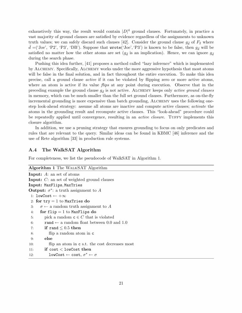
For completeness, we list the pseudocode of WalkSAT in Algorithm 1.

Algorithm 1 The WalkSAT AlgorithmInput: A: an set of atomsInput: C: an set of weighted ground clausesInput: MaxFlips, MaxTriesOutput: σ∗: a truth assignment to A

1: lowCost← +∞2: for try = 1 to MaxTries do3: σ ← a random truth assignment to A4: for flip = 1 to MaxFlips do5: pick a random c ∈ C that is violated6: rand← a random float between 0.0 and 1.07: if rand ≤ 0.5 then8: flip a random atom in c9: else

10: flip an atom in c s.t. the cost decreases most11: if cost < lowCost then12: lowCost← cost, σ∗ ← σ

21

A.5 Marginal Inference of MLNs

In marginal inference, we are given a set of atoms together with a truth assignment to them.The goal is to estimate the marginal probability of this partial assignment. Since this problemis generally intractable, we usually resort to sampling methods. The state-of-the-art marginalinference algorithm of MLNs is MC-SAT [40], which is implemented in both Alchemy and Tuffy.In MC-SAT, each sampling step consists of a call to a heuristic SAT sampler named SampleSAT [45].Essentially, SampleSAT is a combination of simulated annealing and WalkSAT. And so, Tuffy isable to perform marginal inference more efficiently as well.

B Material for Systems

B.1 An Example SQL Query For Grounding

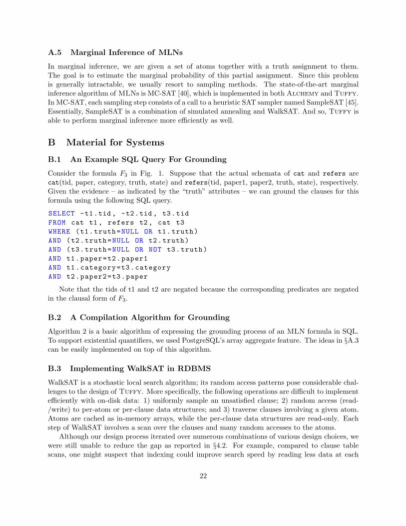
Consider the formula F3 in Fig. 1. Suppose that the actual schemata of cat and refers arecat(tid, paper, category, truth, state) and refers(tid, paper1, paper2, truth, state), respectively.Given the evidence – as indicated by the “truth” attributes – we can ground the clauses for thisformula using the following SQL query.

SELECT -t1.tid , -t2.tid , t3.tidFROM cat t1 , refers t2 , cat t3WHERE (t1.truth=NULL OR t1.truth)AND (t2.truth=NULL OR t2.truth)AND (t3.truth=NULL OR NOT t3.truth)AND t1.paper=t2.paper1AND t1.category=t3.categoryAND t2.paper2=t3.paper

Note that the tids of t1 and t2 are negated because the corresponding predicates are negatedin the clausal form of F3.

B.2 A Compilation Algorithm for Grounding

Algorithm 2 is a basic algorithm of expressing the grounding process of an MLN formula in SQL.To support existential quantifiers, we used PostgreSQL’s array aggregate feature. The ideas in §A.3can be easily implemented on top of this algorithm.

B.3 Implementing WalkSAT in RDBMS

WalkSAT is a stochastic local search algorithm; its random access patterns pose considerable chal-lenges to the design of Tuffy. More specifically, the following operations are difficult to implementefficiently with on-disk data: 1) uniformly sample an unsatisfied clause; 2) random access (read-/write) to per-atom or per-clause data structures; and 3) traverse clauses involving a given atom.Atoms are cached as in-memory arrays, while the per-clause data structures are read-only. Eachstep of WalkSAT involves a scan over the clauses and many random accesses to the atoms.

Although our design process iterated over numerous combinations of various design choices, wewere still unable to reduce the gap as reported in §4.2. For example, compared to clause tablescans, one might suspect that indexing could improve search speed by reading less data at each

22

Algorithm 2 MLN Grounding in SQL

Input: an MLN formula φ = ∨ki=1li where each li is a literal supported by predicate table r(li)

Output: a SQL query Q that grounds φ1: FROM clause of Q includes ‘r(li) ti’ for each literal li2: SELECT clause of Q contains ‘ti.aid’ for each literal li3: For each positive (resp. negative) literal li, there is a WHERE predicate ‘ti.truth 6= true’ (resp.

‘ti.truth 6= false’)4: For each variable x in φ, there is a WHERE predicate that equates the corresponding columns

of ti’s with li containing x5: For each constant argument of li, there is an equal-constant WHERE predicate for table ti6: Form a conjunction with the above WHERE predicates

step. However, we actually found that the cost of maintaining indices often outweighs the benefitprovided by indexing. Moreover, we found it very difficult to get around RDBMS overhead suchas PostgreSQL’s mandatory MVCC.

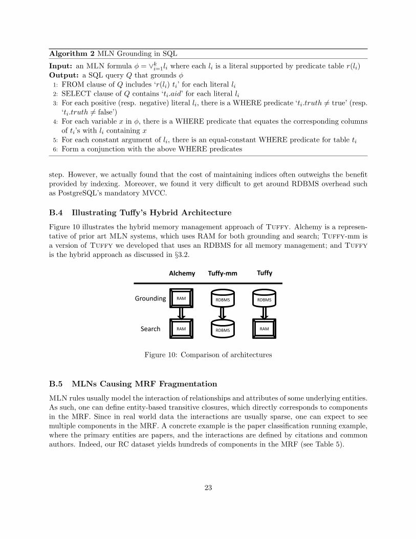
B.4 Illustrating Tuffy’s Hybrid Architecture

Figure 10 illustrates the hybrid memory management approach of Tuffy. Alchemy is a represen-tative of prior art MLN systems, which uses RAM for both grounding and search; Tuffy-mm isa version of Tuffy we developed that uses an RDBMS for all memory management; and Tuffyis the hybrid approach as discussed in §3.2.

RDBMS RAM

RAM RDBMS RAM

RDBMS Grounding

Search

Alchemy Tuffy-mm Tuffy

Figure 10: Comparison of architectures

B.5 MLNs Causing MRF Fragmentation

MLN rules usually model the interaction of relationships and attributes of some underlying entities.As such, one can define entity-based transitive closures, which directly corresponds to componentsin the MRF. Since in real world data the interactions are usually sparse, one can expect to seemultiple components in the MRF. A concrete example is the paper classification running example,where the primary entities are papers, and the interactions are defined by citations and commonauthors. Indeed, our RC dataset yields hundreds of components in the MRF (see Table 5).

23

B.6 Theorem 3.1

of Theorem 3.1. We follow the notations of the theorem. Without loss of generality and for easeof notation, suppose H = 1, . . . , N. Denote by Ω the state space of G. Let Qk ⊆ Ω be theset of states of G where there are exactly k non-optimal components. For any state x ∈ Ω,define H(x) = E[Hx(Q0)], i.e., the expected hitting time of an optimal state from x. Definefk = minx∈Qk

H(x); in particular, f0 = 0. Define gk = fk+1 − fk. For any x, y ∈ Ω, let Pr(x→ y)be the transition probability of WalkSAT, i.e., the probability that next state will be y given currentstate x. Note that Pr(x→ y) > 0 only if y ∈ N(x), where N(x) is the set of states that differ fromx by at most one bit. For any A ⊆ Ω, define Pr(x→ A) =

∑y∈A Pr(x→ y).

For any x ∈ Qk, we have

H(x) = 1 +∑y∈Ω

Pr(x→ y)H(y)

= 1 +∑

t∈−1,0,1

∑y∈Qk+t

Pr(x→ y)H(y)

≥ 1 +∑

t∈−1,0,1

∑y∈Qk+t

Pr(x→ y)fk+t.

DefineP x

+ = Pr(x→ Qk+1), P x− = Pr(x→ Qk−1),

then Pr(x→ Qk) = 1− P x+ − P x

−, and

H(x) ≥ 1 + fk(1− P x+ − P x

−) + fk−1Px− + fk+1P

x+.

Since this inequality holds for any x ∈ Qk, we can fix it to be some x∗ ∈ Qk s.t. H(x∗) = fk.Then gk−1P

x∗− ≥ 1 + gkP

x∗+ , which implies gk−1 ≥ gkP

x∗+ /P x∗

− .Now without loss of generality assume that in x∗, G1, . . . , Gk are non-optimal whileGk+1, . . . , GN

are optimal. Let x∗i be the projection of x∗ on Gi. Then since

P x∗− =

∑k1 vi(x∗i )αi(x∗i )∑N

1 vi(x∗i ), P x∗

+ =

∑Nk+1 vj(x∗j )βj(x∗j )∑N

1 vi(x∗i ),

we have

gk−1 ≥ gk

∑Nk+1 vj(x∗j )βj(x∗j )∑k

1 vi(x∗i )αi(x∗i )≥ gk

r(N − k)k

,

where the second inequality follows from definition of r.For all k ≤ rN/(r + 2), we have gk−1 ≥ 2gk. Since gk ≥ 1 for any k, f1 = g0 ≥ 2rN/(r+2).

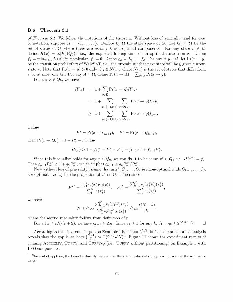
According to this theorem, the gap on Example 1 is at least 2N/3; in fact, a more detailed analysisreveals that the gap is at least

(N−1N2

)≈ Θ(2N/

√N).9 Figure 11 shows the experiment results of

running Alchemy, Tuffy, and Tuffy-p (i.e., Tuffy without partitioning) on Example 1 with1000 components.

9Instead of applying the bound r directly, we can use the actual values of αi, βi, and vi to solve the recurrenceon gk.

24

500

1000

1500

2000

0 20 40 60 80

cost

time (sec)

Performance on Example 1

Tuffy-p (dotted) Alchemy (solid)

Tuffy

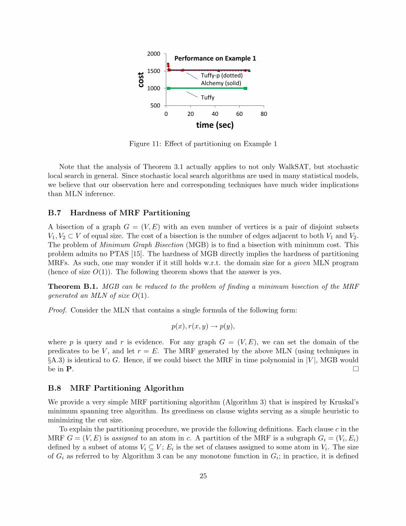
Figure 11: Effect of partitioning on Example 1

Note that the analysis of Theorem 3.1 actually applies to not only WalkSAT, but stochasticlocal search in general. Since stochastic local search algorithms are used in many statistical models,we believe that our observation here and corresponding techniques have much wider implicationsthan MLN inference.

B.7 Hardness of MRF Partitioning

A bisection of a graph G = (V,E) with an even number of vertices is a pair of disjoint subsetsV1, V2 ⊂ V of equal size. The cost of a bisection is the number of edges adjacent to both V1 and V2.The problem of Minimum Graph Bisection (MGB) is to find a bisection with minimum cost. Thisproblem admits no PTAS [15]. The hardness of MGB directly implies the hardness of partitioningMRFs. As such, one may wonder if it still holds w.r.t. the domain size for a given MLN program(hence of size O(1)). The following theorem shows that the answer is yes.

Theorem B.1. MGB can be reduced to the problem of finding a minimum bisection of the MRFgenerated an MLN of size O(1).

Proof. Consider the MLN that contains a single formula of the following form:

p(x), r(x, y)→ p(y),

where p is query and r is evidence. For any graph G = (V,E), we can set the domain of thepredicates to be V , and let r = E. The MRF generated by the above MLN (using techniques in§A.3) is identical to G. Hence, if we could bisect the MRF in time polynomial in |V |, MGB wouldbe in P.

B.8 MRF Partitioning Algorithm

We provide a very simple MRF partitioning algorithm (Algorithm 3) that is inspired by Kruskal’sminimum spanning tree algorithm. Its greediness on clause wights serving as a simple heuristic tominimizing the cut size.

To explain the partitioning procedure, we provide the following definitions. Each clause c in theMRF G = (V,E) is assigned to an atom in c. A partition of the MRF is a subgraph Gi = (Vi, Ei)defined by a subset of atoms Vi ⊆ V ; Ei is the set of clauses assigned to some atom in Vi. The sizeof Gi as referred to by Algorithm 3 can be any monotone function in Gi; in practice, it is defined

25

to be the total number of literals and atoms in Gi. Note that when the parameter β is set to +∞,the output is the connected components of G.

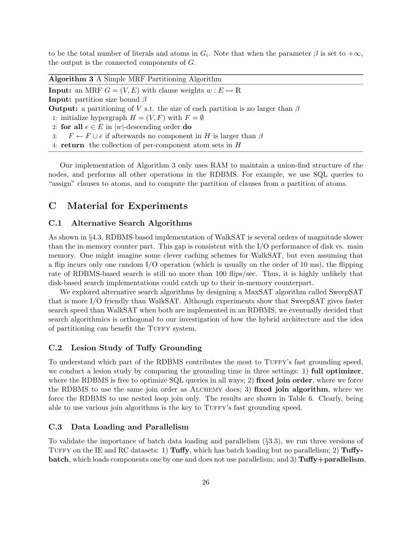
Algorithm 3 A Simple MRF Partitioning Algorithm

Input: an MRF G = (V,E) with clause weights w : E 7→ R

Input: partition size bound βOutput: a partitioning of V s.t. the size of each partition is no larger than β

1: initialize hypergraph H = (V, F ) with F = ∅2: for all e ∈ E in |w|-descending order do3: F ← F ∪ e if afterwards no component in H is larger than β4: return the collection of per-component atom sets in H

Our implementation of Algorithm 3 only uses RAM to maintain a union-find structure of thenodes, and performs all other operations in the RDBMS. For example, we use SQL queries to“assign” clauses to atoms, and to compute the partition of clauses from a partition of atoms.

C Material for Experiments

C.1 Alternative Search Algorithms

As shown in §4.3, RDBMS-based implementation of WalkSAT is several orders of magnitude slowerthan the in-memory counter part. This gap is consistent with the I/O performance of disk vs. mainmemory. One might imagine some clever caching schemes for WalkSAT, but even assuming thata flip incurs only one random I/O operation (which is usually on the order of 10 ms), the flippingrate of RDBMS-based search is still no more than 100 flips/sec. Thus, it is highly unlikely thatdisk-based search implementations could catch up to their in-memory counterpart.

We explored alternative search algorithms by designing a MaxSAT algorithm called SweepSATthat is more I/O friendly than WalkSAT. Although experiments show that SweepSAT gives fastersearch speed than WalkSAT when both are implemented in an RDBMS, we eventually decided thatsearch algorithmics is orthogonal to our investigation of how the hybrid architecture and the ideaof partitioning can benefit the Tuffy system.

C.2 Lesion Study of Tuffy Grounding

To understand which part of the RDBMS contributes the most to Tuffy’s fast grounding speed,we conduct a lesion study by comparing the grounding time in three settings: 1) full optimizer,where the RDBMS is free to optimize SQL queries in all ways; 2) fixed join order, where we forcethe RDBMS to use the same join order as Alchemy does; 3) fixed join algorithm, where weforce the RDBMS to use nested loop join only. The results are shown in Table 6. Clearly, beingable to use various join algorithms is the key to Tuffy’s fast grounding speed.

C.3 Data Loading and Parallelism

To validate the importance of batch data loading and parallelism (§3.3), we run three versions ofTuffy on the IE and RC datasets: 1) Tuffy, which has batch loading but no parallelism; 2) Tuffy-batch, which loads components one by one and does not use parallelism; and 3) Tuffy+parallelism,

26

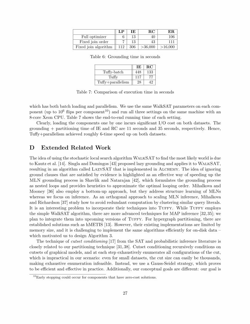
LP IE RC ERFull optimizer 6 13 40 106

Fixed join order 7 13 43 111Fixed join algorithm 112 306 >36,000 >16,000

Table 6: Grounding time in seconds

IE RCTuffy-batch 448 133

Tuffy 117 77Tuffy+parallelism 28 42

Table 7: Comparison of execution time in seconds

which has both batch loading and parallelism. We use the same WalkSAT parameters on each com-ponent (up to 106 flips per component10) and run all three settings on the same machine with an8-core Xeon CPU. Table 7 shows the end-to-end running time of each setting.

Clearly, loading the components one by one incurs significant I/O cost on both datasets. Thegrounding + partitioning time of IE and RC are 11 seconds and 35 seconds, respectively. Hence,Tuffy+parallelism achieved roughly 6-time speed up on both datasets.

D Extended Related Work

The idea of using the stochastic local search algorithm WalkSAT to find the most likely world is dueto Kautz et al. [14]. Singla and Domingos [43] proposed lazy grounding and applies it to WalkSAT,resulting in an algorithm called LazySAT that is implemented in Alchemy. The idea of ignoringground clauses that are satisfied by evidence is highlighted as an effective way of speeding up theMLN grounding process in Shavlik and Natarajan [42], which formulates the grounding processas nested loops and provides heuristics to approximate the optimal looping order. Mihalkova andMooney [36] also employ a bottom-up approach, but they address structure learning of MLNswhereas we focus on inference. As an orthogonal approach to scaling MLN inference, Mihalkovaand Richardson [37] study how to avoid redundant computation by clustering similar query literals.It is an interesting problem to incorporate their techniques into Tuffy. While Tuffy employsthe simple WalkSAT algorithm, there are more advanced techniques for MAP inference [32,35]; weplan to integrate them into upcoming versions of Tuffy. For hypergraph partitioning, there areestablished solutions such as hMETIS [13]. However, their existing implementations are limited bymemory size, and it is challenging to implement the same algorithms efficiently for on-disk data –which motivated us to design Algorithm 3.

The technique of cutset conditioning [17] from the SAT and probabilistic inference literature isclosely related to our partitioning technique [31,38]. Cutset conditioning recursively conditions oncutsets of graphical models, and at each step exhaustively enumerates all configurations of the cut,which is impractical in our scenario: even for small datasets, the cut size can easily be thousands,making exhaustive enumeration infeasible. Instead, we use a Gauss-Seidel strategy, which provesto be efficient and effective in practice. Additionally, our conceptual goals are different: our goal is

10Early stopping could occur for components that have zero-cost solutions.

27

to find an analytic formula that quantifies the effect of partitioning and then, we use this formulato optimize the IO and scheduling behavior of a wide class of local search algorithms; in contrast,prior work focuses on designing new inference algorithms.

Finally, we note that there are statistical-logical frameworks similar to MLNs, such as Proba-bilistic Relational Models [34] and Relational Markov Models [44]. Since inference on those modelsalso requires grounding and search, we believe that the lessons we learned with MLNs will carryover to them, too.

References

[31] D. Allen and A. Darwiche. New advances in inference by recursive conditioning. In UAI03, 2003.

[32] J. Duchi, D. Tarlow, G. Elidan, and D. Koller. Using combinatorial optimization within max-productbelief propagation. NIPS, 2007.

[33] C. Forgy. Rete: A fast algorithm for the many pattern/many object pattern match problem. Artificialintelligence, 1982.

[34] N. Friedman, L. Getoor, D. Koller, and A. Pfeffer. Learning probabilistic relational models. In IJCAI,1999.

[35] R. Gupta, A. Diwan, and S. Sarawagi. Efficient inference with cardinality-based clique potentials. InICML, 2007.

[36] L. Mihalkova and R. Mooney. Bottom-up learning of Markov logic network structure. In ICML, 2007.

[37] L. Mihalkova and M. Richardson. Speeding up inference in statistical relational learning by clusteringsimilar query literals. Inductive Logic Programming, 2010.

[38] T. Park and A. Van Gelder. Partitioning methods for satisfiability testing on large formulas. AutomatedDeduction, 1996.

[39] J. Pearl. Probabilistic reasoning in intelligent systems: networks of plausible inference. 1988.

[40] H. Poon and P. Domingos. Sound and efficient inference with probabilistic and deterministic dependen-cies. In AAAI, 2006.

[41] H. Poon, P. Domingos, and M. Sumner. A general method for reducing the complexity of relationalinference and its application to MCMC. AAAI-08.

[42] J. Shavlik and S. Natarajan. Speeding up inference in Markov logic networks by preprocessing to reducethe size of the resulting grounded network. In IJCAI-09.

[43] P. Singla and P. Domingos. Memory-efficient inference in relational domains. In AAAI ’06.

[44] B. Taskar, P. Abbeel, and D. Koller. Discriminative probabilistic models for relational data. In UAI,2002.

[45] W. Wei, J. Erenrich, and B. Selman. Towards efficient sampling: Exploiting random walk strategies.In AAAI, 2004.

[46] M. Wellman, J. Breese, and R. Goldman. From knowledge bases to decision models. The KnowledgeEngineering Review, 1992.

28