Embed Size (px)
Citation preview
C R A N F I E L D U N I V E R S I T Y S C H O O L O F E N G I N E E R I N G
A s t e r i s A p o s t o l i d i s
T URBINE COOLING AND HE AT TRAN SFE R MODE LLING FOR GAS TURB INE PE RFORMANCE
S IMUL ATION
P h D T h e s i s M a r c h 2 0 1 5
C R A N F I E L D U N I V E R S I T Y S C H O O L O F E N G I N E E R I N G
F u l l T i m e P h D
A c a d e m i c Y e a r 2 0 1 4 - 2 0 1 5
A s t e r i s A p o s t o l i d i s
T URBINE COOLING AND HE AT TRAN SFE R MODE LLING FOR GAS TURB INE PE RFORMANCE
S IMUL ATION
S u p e r v i s o r s :
D r P a n a g i o t i s L a s k a r i d i s P r o f P e r i c l e s P i l i d i s
M a r c h 2 0 1 5
© Cranfield University 2015. All rights reserved. No part of this publication may be reproduced without the written permission of the copyright owner.
Abstract
The successful design of cooling systems for gas turbine engines is a key factor to feasibility of new projects, as the trend for increasing turbine entry temperatures implies requirements for more sophisticated cooling methods. This work focuses on the prediction of cooling performance of turbines, starting from local heat transfer effects at the surface of blades and vanes and expanding to performance simulation of cooled high pressure turbines and engines. In this context, this thesis establishes a new method that investigates the following topics:
• The connection between the gas flow field around a cooled blade or vane and the prediction of cooling requirements of the setup.
• The connection between a detailed gas flow field around a cooled blade or vane and a preliminary estimation of its metal temperature.
• The effect that blade cooling requirements prediction has towards the performance simulation of a cooled turbine and the difference in results between turbine models of different axial resolution.
• A simulation platform that includes the aforementioned topics under a web-based gas turbine performance simulation program.
The first two objectives are tackled by developing a preliminary cooling design framework, which performs the needed convective and conductive heat transfer calculations between the gas and the blade, the blade and the coolant, and within the blade material. The method divides the geometry into a finite number of volumes, where heat transfer calculations are performed for steady-state conditions. One- and two-dimensional results show a good agreement with previous experimental work. The results suggest that chord resolution for blade heat transfer prediction is essential for a more accurate coolant temperature and mass flow rate prediction. In addition, conduction modelling has a dominant effect in heat transfer prediction of blades with steep temperature gradients.
The third objective is achieved by associating the coolant state before mixing with the main stream and the results in turbine performance. The coolant temperature and mass flow rate prediction have a significant impact on turbine work and thermodynamic efficiency, figures highlighted as well for different turbine axial resolution methods. The results suggest that as the coolant heats up through a blade

iv
or vane and eventually mixes with the main flow, it contributes significantly towards the predicted turbine work, affecting as well the overall engine performance results, such as specific fuel consumption and specific thrust. A multistage turbine model is most suitable for capturing these effects, but it requires a number of additional inputs.
Finally, the thesis suggests that a simulation framework such as the aforementioned, it can be of high usability and applicability if implemented on the cloud, rather than locally installed.

v
Acknowledgements
Pursuing a PhD degree is always a challenging task that requires patience, clarity of thinking and definitely some caring people to be around. I was very lucky to be supported by the following persons, to whom I wish to express my gratitude.
First, I would like to express my heartfelt thanks to Dr Panos Laskaridis, not only for being my supervisor but also for his continuous support, effort and for always being available for long (not always technical) discussions. Without his contribution, the present thesis would not have been possible.
I am very thankful to Prof Pericles Pilidis for supporting this thesis with his honest interest, for giving me the opportunity to accomplish this degree and for always being available to listen and advise me through the different phases of this project.
I feel very lucky to have met and worked with Dr Suresh Sampath for those three years at Cranfield. A significant part of this work is outcome of our collaboration and despite the physical distance during most of the time, I consider him as a true friend.
I would like to express my sincere gratitude to Prof Riti Singh, for selecting me to work on the WebEngine project and for his commitment and support throughout the duration of my studies at Cranfield.
A heartfelt “thank you” goes to Prof Anestis Kalfas, for mentoring me during my years at Aristotle University and thereafter. I will never forget his truly inspiring lectures that revealed to me the amazing field of gas turbines.
I am more than grateful to Dr Pavlos Zachos for honouring me with his friendship. I thank him for his honest interest and support, for always being available to discuss anything troubling me. Pavlos was part of my “second family” at Cranfield and this is invaluable.
I would like to honestly thank Dr Theoklis Nikolaidis, Dr Georgios Doulgeris, Dr Bobby Sethi, Dr Uyi Igie and Dr Devaiah Nalianda for their support to this project and their valuable pieces of advice, as friends.
I am thankful to MSc by Research students Tomás Baudín and Atif Shafi for accepting the challenge to be the first people to use the WebEngine for their research, providing us with very useful feedback and suggestions.

vi
The long hours I spent in building 183 would have been very lonely without my officemates and friends Dinos, Eduardo, Alice, Abu and Yiannis. I truly thank them for their solidarity and support.
During my years at Cranfield I have met some people I consider as lifetime friends. Periklis, Elias, Panos, Avgoustinos, Orlando, Thanasis, Yiannis, Giorgos, Fanis, Nikos and Kostis, I deeply thank you for all the moments we shared. You made Cranfield feel like home.
Outside Cranfield, I feel very fortunate to have met my friends and companion for some decades now. Vasios, Panagiotis, Orestis, Kostas, Anastasis, Alexandros, Antigonos, Alexis, Lefteris and Tasos, thank you for your camaraderie. I am looking forward to our next big adventure together!
My life would not be the same without my beloved grandparents Thanasis and Sotiroula, who continuous care and courageously support me. Their love is always a motivation and the summers we spent together in Chalkidiki will always be a sweet memory.
My parents, Christos and Angeliki and my sister, Myrto are the people to whom I owe the biggest “thank you”. For all of my life, they have been a source of love, dignity and courage. They insisted that the biggest asset in life is education and I always keep this in mind as a principle.
Finally, I would like to thank my dearest Margarita for deciding to share her life with me.
Asteris Apostolidis May 2014
vii
Table of Contents
Abstract ................................................................................................................................. iii
Acknowledgements ............................................................................................................. v
List of Figures ...................................................................................................................... xi
List of Tables ....................................................................................................................... xv
Nomenclature .................................................................................................................... xvi
Chapter 1
Introduction .......................................................................................................................... 1
1.1 Scope of Research ....................................................................................................................... 1
1.2 Literature Overview .................................................................................................................. 2
1.2.1 Turbine Blade Heat Transfer ........................................................................................ 2
1.2.2 Multistage Cooled Turbine Simulation .................................................................... 3
1.2.3 Gas Turbine Performance Simulation ...................................................................... 3
1.3 Project Aim and Objectives .................................................................................................... 3
1.4 Thesis Structure ........................................................................................................................... 4
Chapter 2
Project Overview ................................................................................................................. 6
2.1 Current Status and Technology ............................................................................................ 6
2.2 Simulation Platform Overview ............................................................................................. 9
Chapter 3
Turbine Blade Heat Transfer Prediction Overview ................................................. 12
3.1 Introduction ................................................................................................................................ 12
3.2 Heat Transfer Fundamentals .............................................................................................. 13
3.2.1 Thermal Conduction ...................................................................................................... 14
3.2.2 Thermal Convection ...................................................................................................... 15
3.2.3 Heat Transfer by Radiation ........................................................................................ 16
3.3 Two-Dimensional Turbine Flow ....................................................................................... 17
viii
3.4 Turbine Cooling ........................................................................................................................ 18
3.4.1 Introduction ...................................................................................................................... 18
3.4.2 Turbine Blade Materials .............................................................................................. 20
3.4.3 Turbine Cooling Prediction ........................................................................................ 21
Chapter 4
Turbine Blade Heat Transfer Method .......................................................................... 32
4.1 Introduction ................................................................................................................................ 32
4.2 One-Dimensional Method .................................................................................................... 33
4.2.1 Method Background ...................................................................................................... 33
4.2.2 Introduction of Conduction Modelling ................................................................. 35
4.2.3 System Solving Method ................................................................................................ 37
4.2.4 Internal Geometry Modelling .................................................................................... 39
4.2.5 Film Cooling Modelling ................................................................................................ 40
4.3 The Energy Efficient Engine – Method Inputs............................................................ 41
4.4 One-Dimensional Results ..................................................................................................... 45
4.5 One-Dimensional Method Validation ............................................................................. 49
4.6 Two-Dimensional Method ................................................................................................... 51
4.7 Turbine Blade CFD Analysis................................................................................................ 58
4.8 Two-Dimensional Results .................................................................................................... 65
4.9 Two-Dimensional Method Validation ............................................................................ 71
4.10 Three-Dimensional Method ........................................................................................... 72
4.11 Three-Dimensional Results ............................................................................................ 75
4.12 Conclusions and Discussion ........................................................................................... 78
Chapter 5
Multistage Cooled Turbine Simulation ........................................................................ 81
5.1 Gas Turbine Performance Simulation ............................................................................ 81
5.1.1 Introduction ...................................................................................................................... 81
5.1.2 Degrees of Fidelity .......................................................................................................... 82
5.1.3 High Fidelity Components and Integration with the Main Code ............. 84
ix
5.2 The Cooled Turbine – A Literature Survey .................................................................. 86
5.2.1 Introduction ...................................................................................................................... 86
5.2.2 Turbine Aero-Thermodynamics and Efficiency ............................................... 87
5.2.3 Turbine Flow and Sources of Loss .......................................................................... 90
5.2.4 Turbine Modelling .......................................................................................................... 91
5.3 Zero-Dimensional Turbine .................................................................................................. 94
5.3.1 Introduction ...................................................................................................................... 94
5.3.2 Method ................................................................................................................................. 97
5.4 Single-Stage Equivalent Turbine ....................................................................................100
5.4.1 Introduction ....................................................................................................................100
5.4.2 Method ...............................................................................................................................102
5.5 Multistage Turbine ................................................................................................................105
5.5.1 Introduction ....................................................................................................................105
5.5.2 Method ...............................................................................................................................105
5.6 Program Development ........................................................................................................107
5.7 Cooled Turbine Case Study................................................................................................111
5.7.1 Introduction ....................................................................................................................111
5.7.2 Single-Stage HPT Investigation ..............................................................................111
5.7.3 Two-Stage HPT Investigation .................................................................................120
5.7.4 Conclusions ......................................................................................................................130
5.8 Engine Performance Analysis ..........................................................................................131
5.8.1 Introduction ....................................................................................................................131
5.8.2 Method ...............................................................................................................................131
5.8.3 Design Point Case Study ............................................................................................136
5.9 Turbine Cooling Platform Discussion and Applications......................................139
Chapter 6
A Web-based Gas Turbine Performance Simulation Tool ................................... 142
6.1 Introduction ..............................................................................................................................142
6.2 Gas Turbine Performance Simulation ..........................................................................144
x
6.2.1 Simulation Tools Overview ......................................................................................144
6.2.2 Simulation Tools Classification ..............................................................................146
6.3 WebEngine Overview ...........................................................................................................150
6.4 Turbomatch Code Structure .............................................................................................152
6.5 WebEngine Code Structure ...............................................................................................154
6.6 WebEngine Features ............................................................................................................155
6.7 Future Developments...........................................................................................................158
6.8 Conclusions ...............................................................................................................................158
Chapter 7
Conclusions and Future Work ..................................................................................... 160
7.1 Conclusions ...............................................................................................................................160
7.1.1 Turbine Blade Heat Transfer Method .................................................................160
7.1.2 Multistage Cooled Turbine Method......................................................................163
7.1.3 Web-Based Gas Turbine Performance Simulation .......................................165
7.2 Future Work .............................................................................................................................166
References ........................................................................................................................ 168
Appendix
Turbine Blade Heat Transfer (TBHT) Code User Guide.........................................179
xi
List of Figures
2.1: Turbine simulation framework ..................................................................................................... 9
3.1: Turbine Entry Temperature evolution and cooling technologies [Ballal, 2004] 13
3.2: Thermal conduction in molecular level [www.esa.int] ................................................... 14
3.3: Two-Dimensional turbine velocity triangles [Dixon, 2005] ......................................... 17
3.4: Air-Cooled blade modes ................................................................................................................. 19
3.5: Development of turbine cooling technology [Rolls-Royce, 1996] ............................. 19
3.6: Development of turbine blade materials [Schulz, 2003]................................................ 20
3.7: Ainley’s cooling approach [Horlock, 2006]........................................................................... 23
3.8: Garg’s [2000] turbine blade meshing ...................................................................................... 28
4.1: One-Dimensional modelling strategy ...................................................................................... 37
4.2: Meridional HPT view ....................................................................................................................... 43
4.3: E3 HPT NGV and blade dimensions .......................................................................................... 43
4.4: E3 HPT NGV and blade internal configuration .................................................................... 44
4.5: E3 HPT blade cooling mass flow distribution...................................................................... 44
4.6: E3 HPT NGV and blade heat transfer coefficient distribution ..................................... 45
4.7: Level of technology effect .............................................................................................................. 47
4.8: Span gas profile effect ..................................................................................................................... 48
4.9: Span conductivity effect ................................................................................................................. 49
4.10: One-Dimensional validation ...................................................................................................... 50
4.11: Two-Dimensional turbine blade modelling ....................................................................... 54
4.12: Two-dimensional program structure ................................................................................... 55
4.13: CFD model overview ..................................................................................................................... 59
4.14: Grid quality criteria ....................................................................................................................... 60
4.15: CFD boundary conditions overview ...................................................................................... 61
xii
4.16: Vane and blade y+ distribution ................................................................................................ 62
4.17: Stator gas static temperature, Grid sensitivity ................................................................. 62
4.18: Rotor gas static temperature, Grid sensitivity .................................................................. 63
4.19: Vane and blade flow streamlines ............................................................................................ 64
4.20: Stator Mach number and static temperature .................................................................... 64
4.21: Rotor static temperature ............................................................................................................ 65
4.22: Typical Two-dimensional results ........................................................................................... 67
4.23: Axial resolution effect - Stator .................................................................................................. 68
4.24: Chord conductivity effect ............................................................................................................ 69
4.25: Axial resolution effect - Rotor................................................................................................... 70
4.26: Two-Dimensional validation ..................................................................................................... 72
4.27: Finite blade thickness effect ...................................................................................................... 76
4.28: Chord TBC thickness effect ........................................................................................................ 77
4.29: Cooling effectiveness effects ..................................................................................................... 78
5.1: NPSS zooming interconnection platform [Follen, 2000] ............................................... 84
5.2: H-S diagram for the un-cooled turbine stage [Young, 2006] ....................................... 88
5.3: Isentropic and polytropic efficiency, for variable pressure ratio and constant gamma [Dixon, 2005] ............................................................................................................................... 90
5.4: The cooled turbine model of Young and Wilcock [2002b] ............................................ 93
5.5: Single-stage and equivalent zero-dimensional turbine .................................................. 96
5.6: Two-stage and equivalent zero-dimensional turbine...................................................... 96
5.7: Zero-dimensional turbine inputs and outputs .................................................................... 99
5.8: H-S diagram of single-stage equivalent turbine expansion and mixing processes ...........................................................................................................................................................................101
5.9: Schematic diagram of mixing process ...................................................................................102
5.10: H-S diagram of two-stage turbine expansion and mixing processes...................106
5.11: Multistage cooled turbine program information flow ................................................110
xiii
5.12: Power output for different Wc stator/Wc rotor (Parameter: Wc/Wref) ..........112
5.13: Rotor enthalpy drop and mass flow rate for different Wc stator/Wc rotor ....113
5.14: Isentropic and thermodynamic efficiency for different Wc stator/Wc rotor (Parameter: Wc/Wref) ..........................................................................................................................113
5.15: Power output for different Wc stator/Wc rotor (Parameter: Tc) .........................116
5.16: Isentropic and thermodynamic efficiency for different Wc stator/Wc rotor (Parameter: Tc) .........................................................................................................................................117
5.17: H-S diagram of gas and coolant expansions ....................................................................117
5.18: Isentropic and thermodynamic efficiency for different Tc (Parameter: Wc stator/Wc rotor) .......................................................................................................................................118
5.19: Different efficiency definitions for different Wc stator/Wc rotor ........................119
5.20: Power and thermodynamic efficiency comparison between MCT and SSE, for different Wc/Wc max .............................................................................................................................122
5.21: Station-wise Tg comparison between MCT and SSE ...................................................123
5.22: Power output comparison between MCT and SSE for different Wc/Wc max .124
5.23: Efficiency comparison between MCT and SSE for different Wc/Wc max .........125
5.24: Power output comparison between MCT and SSE for different Wc/Wc max (Parameter: Tc) .........................................................................................................................................125
5.25: Thermodynamic efficiency comparison between MCT and SSE for different Wc/Wc max (Parameter: Tc) ..............................................................................................................126
5.26: Thermodynamic efficiency comparison between MCT and SSE for different Tc (Parameter: Wc/Wc max) ....................................................................................................................127
5.27: Total and stage power output for different first stage PR/total PR .....................128
5.28: Power output comparison between MCT and SSE for different first stage PR/total PR ..................................................................................................................................................129
5.29: Thermodynamic efficiency comparison between MCT and SSE for different first stage PR/total PR............................................................................................................................129
5.30: Typical turbine maps (Pachidis, 1999) ..............................................................................133
5.31: Turbine off-design simulation method ..............................................................................134

xiv
5.32: Multistage design-point turbine simulation platform ................................................135
5.33: Isentropic efficiency and power for different HPC pressure ratios and constant thermodynamic efficiency....................................................................................................................137
5.34: “Fish-hook curves” comparison between constant isentropic and thermodynamic efficiency....................................................................................................................138
6.1: Engine off-design simulation webpage .................................................................................144
6.2: GasTurb user interface [Kurzke, 2007] ................................................................................147
6.3: PROOSIS user interface [Alexiou, 2006] ..............................................................................148
6.4: Engine design webpage ................................................................................................................150
6.5: Brick information flow..................................................................................................................153
6.6: WebEngine architecture ..............................................................................................................154
6.7: Engine Specifications File editor webpage .........................................................................156
6.8: Virtual Sensors selection webpage .........................................................................................157
6.9: Power Pland Day Plan webpage ...............................................................................................158
xv
List of Tables
Table 4.1: One-Dimensional Essential Method Inputs ............................................................. 42
Table 4.2: One-Dimensional Inputs ................................................................................................... 46
Table 4.3: Grid Elements ......................................................................................................................... 59
Table 4.4: Two-Dimensional Inputs .................................................................................................. 66
Table 4.5: Three-Dimensional Inputs ............................................................................................... 75
Table 5.1: Cooling streams accounted for different turbine models ................................. 95
Table 5.2: Multistage cooled turbine inputs ................................................................................108
Table 5.3: Station notation ...................................................................................................................108
Table 5.4: Stations Quantities .............................................................................................................109
Table 5.5: P&W E3 Single-Stage turbine inputs.........................................................................112
Table 5.6: MCT and SSE isentropic efficiency comparison for same power output .121
Table 5.7: MCT and SSE inputs ..........................................................................................................122
Table 5.8: Turbine simulation methods comparison ..............................................................131
Table 6.1: Station Vector Variables..................................................................................................152
xvi
Nomenclature
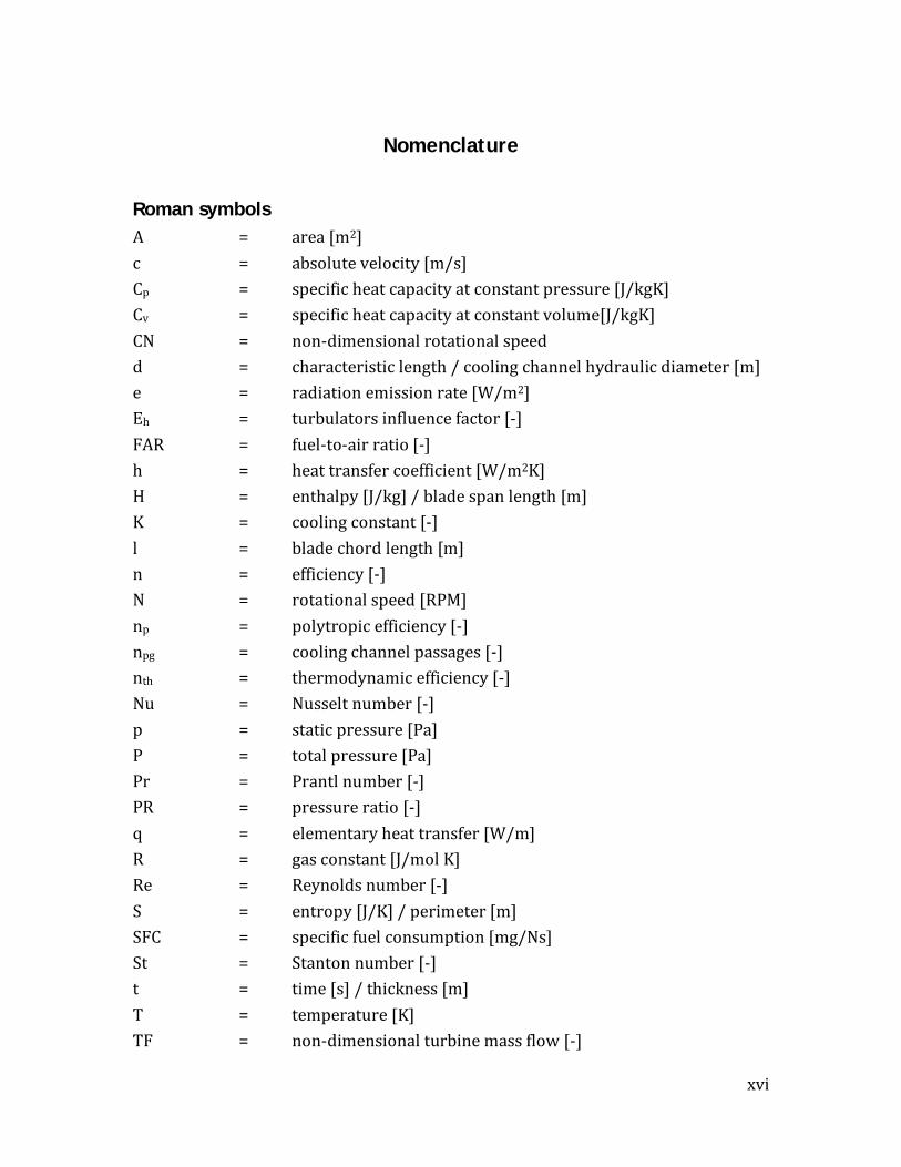
Roman symbols A = area [m2] c = absolute velocity [m/s] Cp = specific heat capacity at constant pressure [J/kgK] Cv = specific heat capacity at constant volume[J/kgK] CN = non-dimensional rotational speed d = characteristic length / cooling channel hydraulic diameter [m] e = radiation emission rate [W/m2] Eh = turbulators influence factor [-] FAR = fuel-to-air ratio [-] h = heat transfer coefficient [W/m2K] H = enthalpy [J/kg] / blade span length [m] K = cooling constant [-] l = blade chord length [m] n = efficiency [-] N = rotational speed [RPM] np = polytropic efficiency [-] npg = cooling channel passages [-] nth = thermodynamic efficiency [-] Nu = Nusselt number [-] p = static pressure [Pa] P = total pressure [Pa] Pr = Prantl number [-] PR = pressure ratio [-] q = elementary heat transfer [W/m] R = gas constant [J/mol K] Re = Reynolds number [-] S = entropy [J/K] / perimeter [m] SFC = specific fuel consumption [mg/Ns] St = Stanton number [-] t = time [s] / thickness [m] T = temperature [K] TF = non-dimensional turbine mass flow [-]
xvii
TW = turbine work [W] U = blade tangential speed [m/s] uT = friction velocity [m/s] v = kinematic viscocity [m2s] V = volume [m3] w = relative velocity [m/s] W = mass flow rate [kg/s] W+ = non-dimensional coolant mass flow rate [-] X = hcSc / hgSg
y+ = non-dimentional wall distance [-] Z = internal geometry technology parameter [-]
Greek symbols α = absolute angle [degrees] αh = empty blade cross-sectional area upon chord squared [-] β = relative angle [degrees] γ = heat capacity ratio [-] ε = emissivity [-] ε0 = cooling effectiveness [-] εfc = film cooling effectiveness [-] λ = thermal conductivity [W/mK] μ = dynamic viscosity [Pa s] ξ = Wc / Wg [-] ρ = density [kg/m3] σ = Stefan-Boltzmann constant [W/m2K4] Ψi = adjacent cooling channels heat transfer factor [-]
Subscripts / Superscripts 1 = stator inlet 2 = stator outlet / rotor inlet 3 = rotor outlet aw = adiabatic wall b = blade c = coolant
xviii
ext = external fc = film cooling g = gas i = inlet i, j = numerical coordinates is = isentropic k = pseudo-time step m = metal / mixed condition me = metal external mi = metal internal MP = mainstream pressure o = outlet ref = reference s = span S = ideal TBC = thermal barrier coating x, y, z = Cartesian coordinates ∞ = far field
Abbreviations ANN = artificial neural networks BBN = Bayesian belief network CFD = computational fluid dynamics E3 = NASA Energy Efficient engine FEM = finite elements method FL = fuzzy logic GA = genetic algorithms HP = high pressure HPT = high pressure turbine HPC = high pressure compressor LES = large eddy simulation LGPA = linear gas path analysis LP = low pressure MCT = multistage cooled turbine NGV = nozzle guide vane
xix
NLGPA = non-linear gas path analysis NTU = number of transfer units OPR = overall pressure ratio SFC = specific fuel consumption SSE = single-stage equivalent TBC = thermal barrier coating TET = turbine entry temperature
1
1 Introduction
1.1 Scope of Research Gas turbines are the dominant propulsion system in modern aviation and a major contributor to the energy industry for almost eight decades. Despite the fact that the main cycle thermodynamic layout remains the same until today, major updates in materials and manufacturing technology enabled series of improvements at the achievable cycle limits, concerning the maximum cycle temperature and pressure.
This path of evolution aims to improved cycle thermal efficiency for the new designs, which keep developing based on higher cycle temperatures even nowadays, offering substantial benefits in both techno-economic and environmental terms. On the other hand, there is solid evidence that the improvement in thermal efficiency with increasing temperature will eventually reach a maximum point [Horlock, 2001a].
Under this consideration, the design of new and more effective cooling systems is an increasingly challenging task, as the amount of available cooling air needs to be kept as minimum as possible. Various methods have been developed for the prediction of blade cooling requirements, ranging from very simplified, to very detailed. The selection of a suitable method is mainly driven by the project design phase, since the availability of detailed blade geometry data is not always possible during the early stages of development.
Literature Overview
2
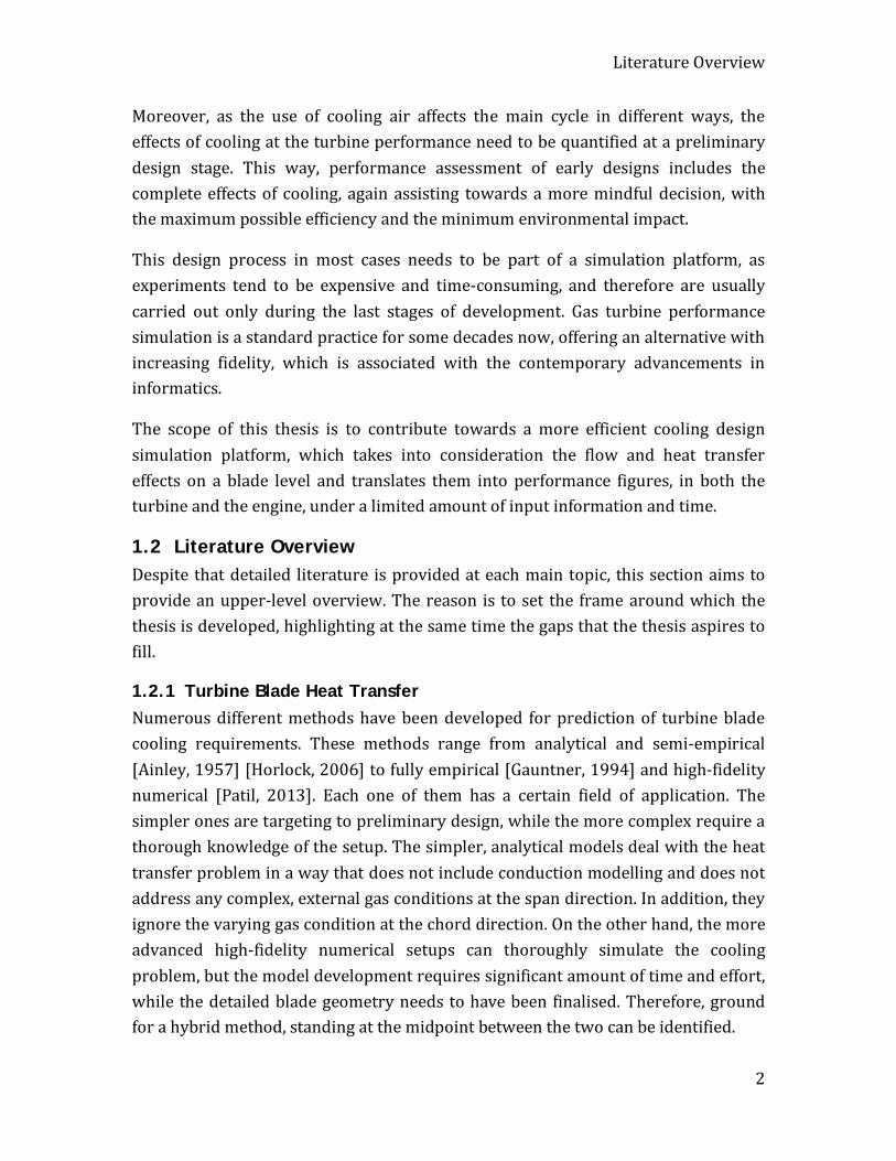
Moreover, as the use of cooling air affects the main cycle in different ways, the effects of cooling at the turbine performance need to be quantified at a preliminary design stage. This way, performance assessment of early designs includes the complete effects of cooling, again assisting towards a more mindful decision, with the maximum possible efficiency and the minimum environmental impact.
This design process in most cases needs to be part of a simulation platform, as experiments tend to be expensive and time-consuming, and therefore are usually carried out only during the last stages of development. Gas turbine performance simulation is a standard practice for some decades now, offering an alternative with increasing fidelity, which is associated with the contemporary advancements in informatics.
The scope of this thesis is to contribute towards a more efficient cooling design simulation platform, which takes into consideration the flow and heat transfer effects on a blade level and translates them into performance figures, in both the turbine and the engine, under a limited amount of input information and time.
1.2 Literature Overview Despite that detailed literature is provided at each main topic, this section aims to provide an upper-level overview. The reason is to set the frame around which the thesis is developed, highlighting at the same time the gaps that the thesis aspires to fill.
1.2.1 Turbine Blade Heat Transfer Numerous different methods have been developed for prediction of turbine blade cooling requirements. These methods range from analytical and semi-empirical [Ainley, 1957] [Horlock, 2006] to fully empirical [Gauntner, 1994] and high-fidelity numerical [Patil, 2013]. Each one of them has a certain field of application. The simpler ones are targeting to preliminary design, while the more complex require a thorough knowledge of the setup. The simpler, analytical models deal with the heat transfer problem in a way that does not include conduction modelling and does not address any complex, external gas conditions at the span direction. In addition, they ignore the varying gas condition at the chord direction. On the other hand, the more advanced high-fidelity numerical setups can thoroughly simulate the cooling problem, but the model development requires significant amount of time and effort, while the detailed blade geometry needs to have been finalised. Therefore, ground for a hybrid method, standing at the midpoint between the two can be identified.

Project Aim and Objectives
3
1.2.2 Multistage Cooled Turbine Simulation There are different approaches in turbine modelling, as part of gas turbine performance simulation programs. As cooling flows are mixing with the gas stream in various axial stations along the turbine, the composition and mass flow of the working fluid changes as well. When a turbine is modelled as zero-dimensional [MacMillan, 1974] or single-stage equivalent [Alexiou, 2006], a certain error is introduced to turbine calculations, as the influence of cooling flows is not correctly calculated, for multi-stage cooled turbines. The only way that this can be addressed is with the development of multi-stage models, where the coolant/gas mixing takes place at the actual axial position, as with the real engine. Such higher fidelity turbine models can be either integrated to the main code, or they can run externally. In any case, a multi-stage model is capable of calculating the thermodynamic efficiency of a turbine as well, a useful figure for the evaluation of the performance of a cooled turbine, as it includes the effects of cooling, compared to more classic efficiency definitions.
1.2.3 Gas Turbine Performance Simulation There are a number of commercial gas turbine simulation codes, each targeting to a different audience. Programs of fixed structure are more oriented to students and teaching applications, whereas more complex codes of interchangeable components and open architecture are targeting to research applications and design projects. Moreover, there are programs more suitable for the aero engine market, or other programs designed for the simulation of complex industrial setups. A common feature that someone could identify is the need for local installation. This may be a restricting factor for many users, as the need for mobility and remote data accessibility is in constant rise, combined with the recent internet evolutions.
1.3 Project Aim and Objectives The aim of this project is to develop a cooling simulation framework, starting from local blade heat transfer effects and expanding to the overall turbine and engine performance. This way, the blade cooling configuration of a new design can be quickly assessed in terms of feasibility and environmental impact, or inversely, the specifications requirements for a new cooling system to be set according to the desired performance.
Thesis Structure
4
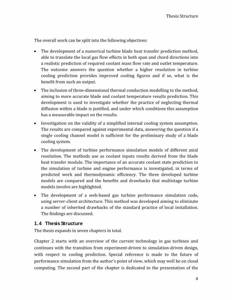
The overall work can be split into the following objectives:
• The development of a numerical turbine blade heat transfer prediction method, able to translate the local gas flow effects in both span and chord directions into a realistic prediction of required coolant mass flow rate and outlet temperature. The outcome answers the question whether a higher resolution in turbine cooling prediction provides improved cooling figures and if so, what is the benefit from such an output.
• The inclusion of three-dimensional thermal conduction modelling to the method, aiming to more accurate blade and coolant temperature results prediction. This development is used to investigate whether the practice of neglecting thermal diffusion within a blade is justified, and under which conditions this assumption has a measurable impact on the results.
• Investigation on the validity of a simplified internal cooling system assumption. The results are compared against experimental data, answering the question if a single cooling channel model is sufficient for the preliminary study of a blade cooling system.
• The development of turbine performance simulation models of different axial resolution. The methods use as coolant inputs results derived from the blade heat transfer module. The importance of an accurate coolant state prediction to the simulation of turbine and engine performance is investigated, in terms of predicted work and thermodynamic efficiency. The three developed turbine models are compared and the benefits and drawbacks that multistage turbine models involve are highlighted.
• The development of a web-based gas turbine performance simulation code, using server-client architecture. This method was developed aiming to eliminate a number of inherited drawbacks of the standard practice of local installation. The findings are discussed.
1.4 Thesis Structure The thesis expands in seven chapters in total.
Chapter 2 starts with an overview of the current technology in gas turbines and continues with the transition from experiment-driven to simulation-driven design, with respect to cooling prediction. Special reference is made to the future of performance simulation from the author’s point of view, which may well be on cloud computing. The second part of the chapter is dedicated to the presentation of the
Thesis Structure
5
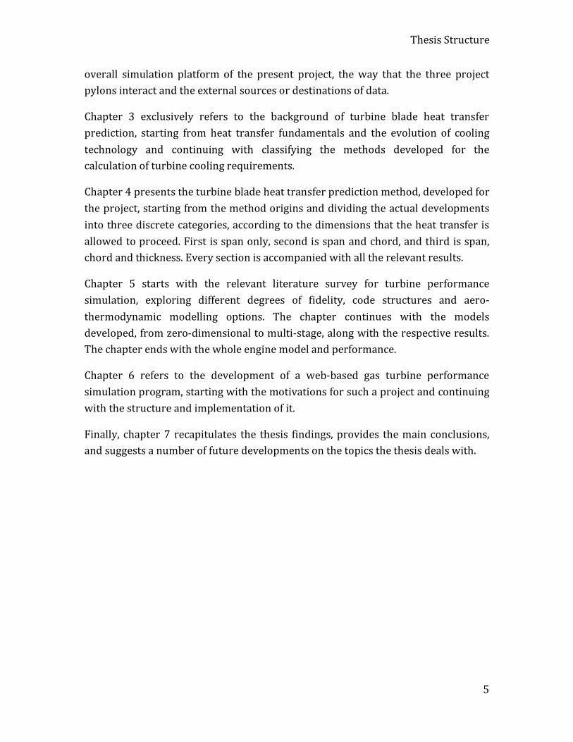
overall simulation platform of the present project, the way that the three project pylons interact and the external sources or destinations of data.
Chapter 3 exclusively refers to the background of turbine blade heat transfer prediction, starting from heat transfer fundamentals and the evolution of cooling technology and continuing with classifying the methods developed for the calculation of turbine cooling requirements.
Chapter 4 presents the turbine blade heat transfer prediction method, developed for the project, starting from the method origins and dividing the actual developments into three discrete categories, according to the dimensions that the heat transfer is allowed to proceed. First is span only, second is span and chord, and third is span, chord and thickness. Every section is accompanied with all the relevant results.
Chapter 5 starts with the relevant literature survey for turbine performance simulation, exploring different degrees of fidelity, code structures and aero-thermodynamic modelling options. The chapter continues with the models developed, from zero-dimensional to multi-stage, along with the respective results. The chapter ends with the whole engine model and performance.
Chapter 6 refers to the development of a web-based gas turbine performance simulation program, starting with the motivations for such a project and continuing with the structure and implementation of it.
Finally, chapter 7 recapitulates the thesis findings, provides the main conclusions, and suggests a number of future developments on the topics the thesis deals with.

6
2 Project Overview
2.1 Current Status and Technology Gas turbine engines are in constant development for eight decades now, a period of time during which vast improvements took place in design, operation and manufacturing [Ballal, 2004]. Meanwhile, gas turbine industry has been evolved into an important sector of the global economy, with great influence and constant growth [Birch, 2000].
Under these conditions, competition increased as well, being a driving force for further improvements in all aspects, from shorter development time, to engines of higher efficiencies, and from improved manufacturability, to lower production costs. At the same time, increasingly stricter environmental legislation and the need for improved reliability are equally important driving forces for the future of the whole industry [Green, 2003].
During the past, the development of new engine and component designs was greatly dependent on experimental testing of prototypes, combined with empirical knowledge, gained after years of experience. The thorough testing of numerous engine and component prototypes can be an expensive and time-consuming task, especially when timetables are strict. At the same time, the vast progress of informatics and computer technology made computer simulations increasingly applicable and popular among designers [Follen, 2000]. This evolution was more capitalised during the last two decades, when flow, mechanical integrity and
Current Status and Technology
7
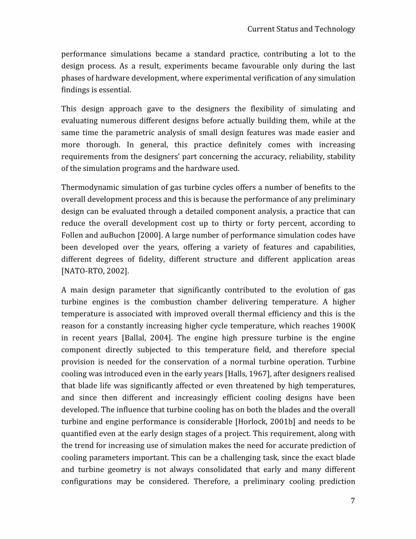
performance simulations became a standard practice, contributing a lot to the design process. As a result, experiments became favourable only during the last phases of hardware development, where experimental verification of any simulation findings is essential.
This design approach gave to the designers the flexibility of simulating and evaluating numerous different designs before actually building them, while at the same time the parametric analysis of small design features was made easier and more thorough. In general, this practice definitely comes with increasing requirements from the designers’ part concerning the accuracy, reliability, stability of the simulation programs and the hardware used.
Thermodynamic simulation of gas turbine cycles offers a number of benefits to the overall development process and this is because the performance of any preliminary design can be evaluated through a detailed component analysis, a practice that can reduce the overall development cost up to thirty or forty percent, according to Follen and auBuchon [2000]. A large number of performance simulation codes have been developed over the years, offering a variety of features and capabilities, different degrees of fidelity, different structure and different application areas [NATO-RTO, 2002].
A main design parameter that significantly contributed to the evolution of gas turbine engines is the combustion chamber delivering temperature. A higher temperature is associated with improved overall thermal efficiency and this is the reason for a constantly increasing higher cycle temperature, which reaches 1900K in recent years [Ballal, 2004]. The engine high pressure turbine is the engine component directly subjected to this temperature field, and therefore special provision is needed for the conservation of a normal turbine operation. Turbine cooling was introduced even in the early years [Halls, 1967], after designers realised that blade life was significantly affected or even threatened by high temperatures, and since then different and increasingly efficient cooling designs have been developed. The influence that turbine cooling has on both the blades and the overall turbine and engine performance is considerable [Horlock, 2001b] and needs to be quantified even at the early design stages of a project. This requirement, along with the trend for increasing use of simulation makes the need for accurate prediction of cooling parameters important. This can be a challenging task, since the exact blade and turbine geometry is not always consolidated that early and many different configurations may be considered. Therefore, a preliminary cooling prediction

Current Status and Technology
8
method can be of high interest for this kind of applications, and the present work is proposing one.
At the same time, as turbine performance is highly affected by cooling, there is a need for higher fidelity prediction of the influence that cooling has in both the turbine and ultimately, the engine. As most gas turbine performance simulation codes were developed as zero-dimensional [NATO-RTO, 2002], not providing information about the internal operation of components, the prediction of cooling influence is less accurately addressed [Alexiou, 2006]. The development of a method able to break down the turbine in axial stations and allocate the different cooling streams, investigating their influence at the final performance result is of significant importance, again to assess the benefits or drawbacks of different cooling designs. And this is because cooling has an adverse effect on the engine thermal efficiency, which may be dominant in modern, heavily-cooled designs [Horlock, 2001a]. At this stage, it is important to remind that a more efficient design is translated into a more financially attractive engine, which makes the final product more feasible for potential customers. Therefore, the preliminary design decisions have a great impact at the commercial aspects of the product, making the simulation methods of great importance.
As there are many different gas turbine performance simulation tools available, each one of them targets to a certain audience. In general, performance simulation programs can be either of fixed or modular structure, with the second approach making possible an interconnection with other, external codes. This must be the case for a cooling prediction method, which needs first to be associated with a higher resolution turbine simulation model and both of them with an engine performance code.
At the internet era, remote data access and transfer have been proved to be of great importance, not only for the gas turbine industry, but in general. There are examples of gas turbine simulation users where local installation, along with an appropriate program configuration proved to be impediments for a wider applicability. In academia, such users may be part time or distant learning students, short course delegates, or even full time students that require access from their place of residence. The same restrictions apply to engineering professionals, which may frequently travel and work from remote facilities, but at the same time require access to their simulation and diagnostics data on site. A response to such requirements can be a key point for the future of gas turbine performance
Simulation Platform Overview
9
simulation and even more if a modular structure facilitates the communication with external design tools, such as the aforementioned ones.
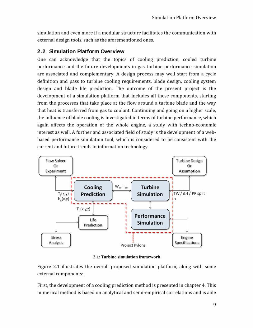
2.2 Simulation Platform Overview One can acknowledge that the topics of cooling prediction, cooled turbine performance and the future developments in gas turbine performance simulation are associated and complementary. A design process may well start from a cycle definition and pass to turbine cooling requirements, blade design, cooling system design and blade life prediction. The outcome of the present project is the development of a simulation platform that includes all these components, starting from the processes that take place at the flow around a turbine blade and the way that heat is transferred from gas to coolant. Continuing and going on a higher scale, the influence of blade cooling is investigated in terms of turbine performance, which again affects the operation of the whole engine, a study with techno-economic interest as well. A further and associated field of study is the development of a web-based performance simulation tool, which is considered to be consistent with the current and future trends in information technology.
2.1: Turbine simulation framework
Figure 2.1 illustrates the overall proposed simulation platform, along with some external components:
First, the development of a cooling prediction method is presented in chapter 4. This numerical method is based on analytical and semi-empirical correlations and is able
Simulation Platform Overview
10
to provide the cooling requirements of a turbine blade or vane, along with the coolant and blade temperatures. The method requires the temperature and heat transfer coefficient of the surrounding gas as inputs, information that may derive from experimental or numerical sources. Then, based on some basic information about the blade geometry and with an intentionally simplified internal cooling channel, a computationally light process is completed, providing results not only at the blade span, but at the blade chord and thickness directions as well. A number of case studies for all dimensions complete the chapter, along with validation at the span and chord directions.
The output of the method can be used for blade creep analysis and life prediction, in the case of blade temperature calculations, when combined with stress analysis. In addition, the coolant calculations are used as inputs for a further cycle calculation.
Chapter 5 is referred to the one-dimensional multistage cooled turbine performance simulation method, developed to account the effects of cooling at the turbine operation. The coolant mass flow and temperature, as calculated from the method of chapter 4, when rejoining the main cycle can greatly affect the gas enthalpy and have a significant effect on the power output. Moreover, the importance of thermodynamic efficiency [Young, 2006] is investigated, since it can be more indicative of the overall turbine performance, as it includes the effects of cooling in contrast with the isentropic efficiency which describes the level of the expansion technology. Two separate cases are explored and compared, the first with a single-stage and the second with a two-stage high pressure turbine, where the findings on stage cooling allocation greatly supports the need for higher fidelity turbine models when the effects of cooling are considered. In order such a simulation to take place, an assumption is required, for the work or enthalpy drop or pressure ratio allocation between the separate stages [Kurzke, 2002]. Moreover, an individual stage isentropic efficiency is required in each case.
The turbine outputs can subsequently used for overall engine cycle calculations. Indeed, as the virtual turbine is ultimately part of an engine simulation tool, the effects of cooled turbine simulation are evaluated in respect to a cycle investigation for a new engine design. In order such investigation to take place, the technical specifications for all the other parts of the engine are required, apparently.
Finally, as earlier denoted, the author’s point of view for the future developments in gas turbine performance simulation programs, but also in general, is that local
Simulation Platform Overview
11
installation of programs will keep shrinking, as most of them will eventually pass to cloud computing. The last part of the project, presented in chapter 6, refers to the development of a web-based gas turbine simulation program, known as Turbomatch WebEngine. The WebEngine is the client-server version of a well-established performance simulation computer code, developed within Cranfield University for almost forty years and currently providing a large amount of technical features. Wrapped on an attractive and user-friendly environment, the WebEngine is ideal for distance learning applications or for remote access from field engineers, as explained in paragraph 2.1. Moreover, the modular structure of the core solver permits future developments of the tool that can include the outcome of the work presented in chapters 4 and 5.
Overall, the three pylons of this piece of work are developed in a way that permits their consideration as a common framework. This framework is able to investigate the performance of cooled turbines in both microscopic and macroscopic level, ideal for preliminary investigation of heavily cooled cycles, where cooling has a great influence. Additionally, blade temperature prediction may very well be a starting point for the consideration of blade life, especially when qualitative comparison among different designs is intended. Last, as society progresses towards an information-oriented direction, cloud computing has a dominant role and a web-based performance simulation tool may be the best platform for the applicability of this work.
12
3 Turbine Blade Heat Transfer Prediction Overview
3.1 Introduction Throughout the last eighty years of development, gas turbine engines have been improved in all aspects. Thrust increased to remarkable levels, while at the same time the efficiency, maintainability and the environmental impact on a life-cycle level were significantly improved compared to the machines of the early years [Ballal, 2004]. A lot of effort was put in various areas, as improvements in all parts of the engine contributed to the success of modern designs.
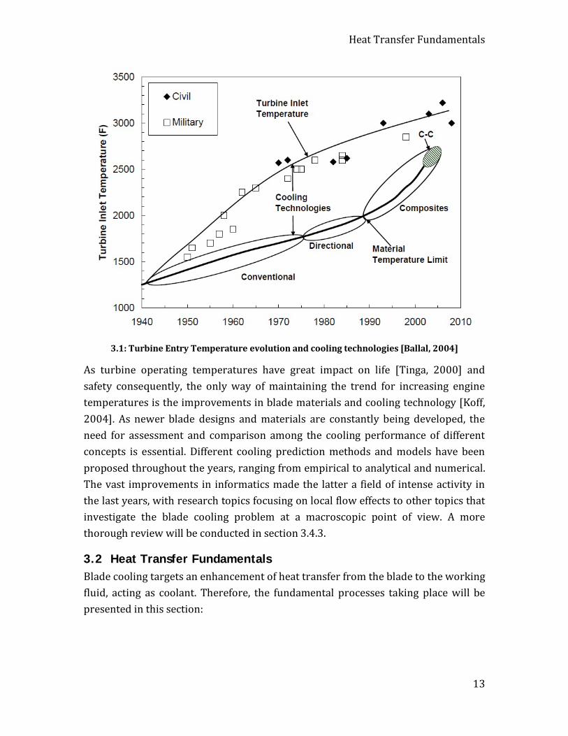
A big step towards this direction is the improvements in engine pressure ratio and combustion temperature that still keep increasing, as illustrated in figure 3.1. The overall thermal efficiency improves as well with increasing temperature, but this comes with a penalty: The need for increased in quantity and improved in efficiency cooling. Indeed, with Turbine Entry Temperatures that reach 1900K for new designs, the materials’ thermal threshold has been far exceeded.
Heat Transfer Fundamentals
13
3.1: Turbine Entry Temperature evolution and cooling technologies [Ballal, 2004]
As turbine operating temperatures have great impact on life [Tinga, 2000] and safety consequently, the only way of maintaining the trend for increasing engine temperatures is the improvements in blade materials and cooling technology [Koff, 2004]. As newer blade designs and materials are constantly being developed, the need for assessment and comparison among the cooling performance of different concepts is essential. Different cooling prediction methods and models have been proposed throughout the years, ranging from empirical to analytical and numerical. The vast improvements in informatics made the latter a field of intense activity in the last years, with research topics focusing on local flow effects to other topics that investigate the blade cooling problem at a macroscopic point of view. A more thorough review will be conducted in section 3.4.3.
3.2 Heat Transfer Fundamentals Blade cooling targets an enhancement of heat transfer from the blade to the working fluid, acting as coolant. Therefore, the fundamental processes taking place will be presented in this section:

Heat Transfer Fundamentals
14
3.2.1 Thermal Conduction The term conduction describes the heat transfer by the interaction of neighbouring molecules with different energy contents. Let us assume two plates of different temperature, separated by an amount of gas in still condition. The interaction of the gas molecules with the hot plate lead to a gas temperature gradient between the two extremes. A higher temperature implies higher molecular energy levels. Therefore, when two molecules of different temperature interact, energy is transferred from the higher energy to the lower energy ones. In other words, when a temperature gradient exists, energy is transferred by conduction along the direction of descending temperature, described as thermal diffusion as well.
3.2: Thermal conduction in molecular level [www.esa.int]
The mechanism of thermal conduction exists in all three phases of matter, despite the different structure and kinetics in a molecular level. The energy transfer along a descending temperature remains present, but quantitatively it is higher in solids, due to the lower distance and the higher interaction between the molecules [Lienhard, 2012].
These observations can be quantified with the understanding of the thermal conduction kinetics equation, which is known as the equation of Fourier, which takes the following form for one-dimensional conduction:
dTqdx
λ= − (3.1)
The equation of Fourier for one dimension states that the amount of energy transferred by conduction is analogous to the temperature gradient, but with an opposite direction. The lamda term is conductivity, a material property that defines the rate of heat transfer.
Heat Transfer Fundamentals
15
3.2.2 Thermal Convection The term convection describes the heat transfer to or from a fluid in motion. In other words, in this case the macroscopic motion of the fluid contributes as well to the transfer of energy, on top of the heat transfer due to molecular motion.
As known, when a viscous fluid flows over a surface, a velocity boundary layer forms. In addition to the viscous boundary layer, a thermal boundary layer is formed as well, where the fluid temperature gradually changes from surface temperature to the temperature of the far field [Lakshminarayana, 1995]. The thickness of the thermal boundary layer differs from the thickness of the velocity boundary layer and it can be anywhere from lower to higher, in comparison between the two. The convective heat transfer is present in any case where there is a temperature gradient between a surface and a moving fluid.
Thermal convection can be classified to forced and natural. At the former, the fluid motion is a result of an external source, whereas at the latter the fluid motion is a result of buoyancy due to non-uniformities at the fluid composition and density, or in multi-phase problems.
Independently of the mechanisms that cause the fluid motion, the convective heat transfer is described by Newton’s law of cooling:
( )q h T T∞= − (3.2)
According to the convection equation, the relation between the amount of heat transferred and the temperature gradient is between the fluid and the surface is linear. Heat transfer coefficient h includes all the factors that have effect on the amount of heat transferred by convection. Therefore, the boundary layer form, the geometry, the flow properties, they all influence heat transfer coefficient h. As a result, the determination of heat transfer coefficient on a specific problem is crucial and very influential to the results.
Heat transfer coefficient h is many times expressed as Nusselt number [Hodge, 1960a, 1960b] [Garg, 1997]. The definitions of the most common non-dimensional numbers, relevant to the heat transfer problem, follow:
Nusselt number
Nusselt number expresses the ratio between convective and conductive heat transfer across a boundary. As convection includes both diffusion and advection, on

Heat Transfer Fundamentals
16
a laminar boundary layer Nusselt number is low, at a unity magnitude. As the flow transits to turbulent, Nusselt number increases significantly due to mixing, that increases the temperature gradient as well across the boundary layer.
h dNuλ
= ( 3.3)
Stanton number
Stanton number is widely used as well in forced convection problems, as it expresses the ratio between the convective heat transfer coefficient and the heat capacity of the fluid.
p
hStcCρ
= (3.4)
Reynolds number
Reynolds number is an expression of the flow inertia forces compared with the viscous forces within the fluid. It is used to predict the type of flow and the patterns associated with it, in different kinds of problems.
Re c dρµ
= (3.5)
Prandtl number
Finally, Prandtl number expresses the ratio between the momentum and thermal diffusivity. It should be noted that there is no physical length scale accounted, and therefore this is a property of the fluid, in contrast with the previous numbers, being properties of a specific flow.
Pr pCµλ
= (3.6)
3.2.3 Heat Transfer by Radiation Matter emits radiation, depending on temperature and other properties and independently from the matter phase. Heat transfer by radiation is associated with changes in the electrons structure of molecules or atoms. The energy of radiation is transferred via electromagnetic waves or in other words, photons. Therefore, there

Two-Dimensional Turbine Flow
17
the presence of a medium for heat transfer by radiation is not necessary. As a result, vacuum is where heat transfer by radiation is most efficient [Howell, 2002].
The Stefan-Boltzmann equation describes the rate of heat transfer by radiation:
4e Tε σ= (3.7)
Where e is the rate of radiation emission, ε is the emissivity (unity for a black body), σ is the Stefan-Boltzmann constant and T is the absolute temperature. In other words, emissivity is the ratio between the radiation emissions of an object upon the radiation emission of a black body.
The models developed at this chapter include both heat transfer by conduction and convection, neglecting the heat transfer by radiation.
3.3 Two-Dimensional Turbine Flow A two-dimensional approach offers a simplification at the study of turbine flow properties. The two main approximations are referred to a zero radial velocity, and a uniform flow along the circumferential direction.
An axial turbine stage is composed by a row of fixed guide vanes (stator) and a row of moving blades (rotor), as illustrated in figure 3.3.
3.3: Two-Dimensional turbine velocity triangles [Dixon, 2005]

Turbine Cooling
18
The flow is assumed to pass through the stator row with an absolute velocity c1 and an angle α1, being accelerated to an absolute velocity c2 and an angle α2 from the axial direction. Passing to the relative coordinate system attached to the rotor, the rotor relative inlet velocity is w2, with a relative angle β2. The blade is assumed to have a linear (derived from the tangential in reality) speed U. The fluid exits the rotor at a relative speed w3, which is translated to c3 at the absolute system and angles α3 and β3, respectively, if added the vector of blade velocity U.
For this set of calculations, a constant axial velocity is assumed at all stations, which converts the equation of continuity as following:
1 1 1 2 2 2 3 3 31 1 2 2 3 3
1 2 3
x x x
x x x
A c A c A cA A A
c c c
ρ ρ ρρ ρ ρ
= = = == =
(3.8)
Constant axial velocity is an assumption often used in preliminary turbine design.
3.4 Turbine Cooling
3.4.1 Introduction The cooling of turbine blades is a necessity for all modern gas turbine engines, as a high portion of engine failures are related to blade failures [Tinga, 2001]. Most of these problems are associated with thermal stresses in turbine blades, where creep is a very significant factor in blade plastic deformation.
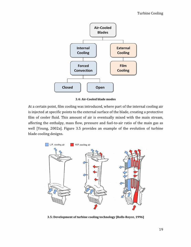
For the prevention of such failures, a better blade thermal performance is required, a fact that drove the cooling research towards more sophisticated designs. For blades cooled with air, the first designs were internal forced convective cooling, that became more advanced with time. More channels were added, along with multiple sources of cooling air. Figure 3.4 illustrates the modes of cooling for air-cooled blades:
Turbine Cooling
19
3.4: Air-Cooled blade modes
At a certain point, film cooling was introduced, where part of the internal cooling air is injected at specific points to the external surface of the blade, creating a protective film of cooler fluid. This amount of air is eventually mixed with the main stream, affecting the enthalpy, mass flow, pressure and fuel-to-air ratio of the main gas as well [Young, 2002a]. Figure 3.5 provides an example of the evolution of turbine blade cooling designs.
3.5: Development of turbine cooling technology [Rolls-Royce, 1996]
Turbine Cooling
20
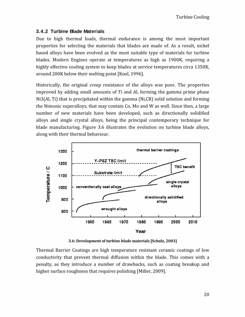
3.4.2 Turbine Blade Materials Due to high thermal loads, thermal endurance is among the most important properties for selecting the materials that blades are made of. As a result, nickel based alloys have been evolved as the most suitable type of materials for turbine blades. Modern Engines operate at temperatures as high as 1900K, requiring a highly effective cooling system to keep blades at service temperatures circa 1350K, around 200K below their melting point [Kool, 1996].
Historically, the original creep resistance of the alloys was poor. The properties improved by adding small amounts of Ti and Al, forming the gamma prime phase Ni3(Al, Ti) that is precipitated within the gamma (Ni,CR) solid solution and forming the Nimonic superalloys, that may contain Co, Mo and W as well. Since then, a large number of new materials have been developed, such as directionally solidified alloys and single crystal alloys, being the principal contemporary technique for blade manufacturing. Figure 3.6 illustrates the evolution on turbine blade alloys, along with their thermal behaviour.
3.6: Development of turbine blade materials [Schulz, 2003]
Thermal Barrier Coatings are high temperature resistant ceramic coatings of low conductivity that prevent thermal diffusion within the blade. This comes with a penalty, as they introduce a number of drawbacks, such as coating breakup and higher surface roughness that requires polishing [Miller, 2009].

Turbine Cooling
21
3.4.3 Turbine Cooling Prediction
3.4.3.1 Introduction Throughout years of development, new gas turbine engines keep running at increasingly higher temperatures, while demanding higher amounts of cooling air bled from the cold part of the engine, in order to maintain the mechanical integrity of the components downstream the combustion chamber. This demand for higher amount of cooling air extraction is directly associated with a penalty at the overall thermal efficiency of the cycle [Horlock, 2001a]. At the same time, the level of technology used for the blade and disc cooling systems has significantly increased, by designing more sophisticated layouts for the internal cooling channel network of the blade and more effective film cooling configurations.
At the preliminary design stage of a cycle, little knowledge exists for the actual component design. An extended number of different scenarios is examined, with only few of them actually manufactured and tested [Follen, 2000]. Since the amount of required cooling air is an essential figure for the assessment of the engine thermal efficiency and feasibility, designers are based on different kinds of methods for this kind of prediction, as referred in [Simoneau, 1993]. These methods can be classified according to their fundamental approach to analytical and semi-empirical [Ainley, 1957] [Horlock, 1973] [Holland, 1980] [Consonni, 1992] [Torbidoni, 2004a] [Torbidoni, 2004b] [Horlock, 2006], empirical [Gauntner, 1994] and high-fidelity numerical [Garg, 1999] [Tinga, 2001] [Lakehal, 2001] [Wheeler, 2011] [Kegalj, 2007]. Additionally, the methods differ in the provided blade resolution. The number of heat transfer directions used can be anywhere from zero for low fidelity empirical methods [Gauntner, 1994] to three, for detailed numerical simulations using CFD [Rosic, 2011] [Wheeler, 2011] [Patil, 2013], FEM [Tinga, 2000] or conjugate modeling [Duchaine, 2009] that combines the two. Of course, the intended type and use of the results is an essential parameter, as the time needed for model development and execution differs a lot among them.
A more thorough description follows:
3.4.3.2 Analytical and Semi-Empirical Models The model developed by Ainley [1957] was a significant first step towards the further development of a series of analytical models. The model results include the calculation of the blade temperature distribution Tb(y) and the coolant temperature distribution Tc(y) in the span direction of thin-walled blades cooled by internal
Turbine Cooling
22
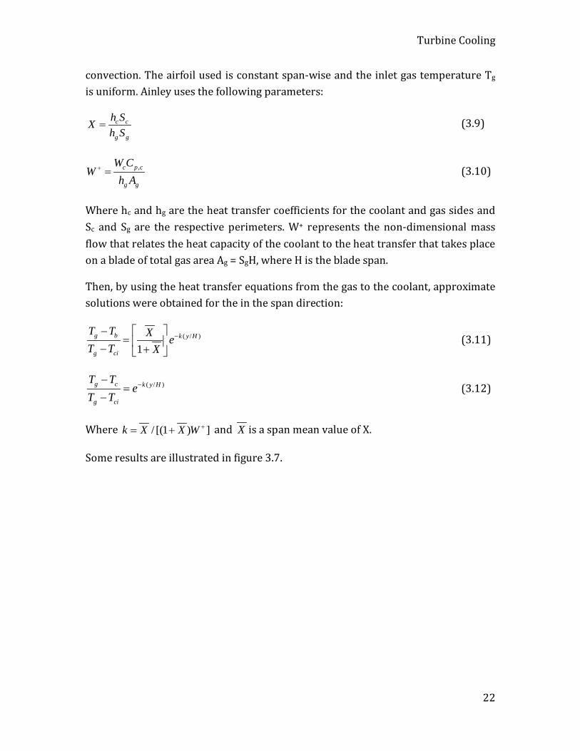
convection. The airfoil used is constant span-wise and the inlet gas temperature Tg is uniform. Ainley uses the following parameters:
c c
g g
h SXh S
= (3.9)
,c p c
g g
W CW
h A+ = (3.10)
Where hc and hg are the heat transfer coefficients for the coolant and gas sides and Sc and Sg are the respective perimeters. W+ represents the non-dimensional mass flow that relates the heat capacity of the coolant to the heat transfer that takes place on a blade of total gas area Ag = SgH, where H is the blade span.
Then, by using the heat transfer equations from the gas to the coolant, approximate solutions were obtained for the in the span direction:
( / )
1g b k y H
g ci
T T X eT T X
−− = − +
(3.11)
( / )g c k y H
g ci
T Te
T T−−
=−
(3.12)
Where / [(1 ) ]k X X W += + and X is a span mean value of X.
Some results are illustrated in figure 3.7.
Turbine Cooling
23
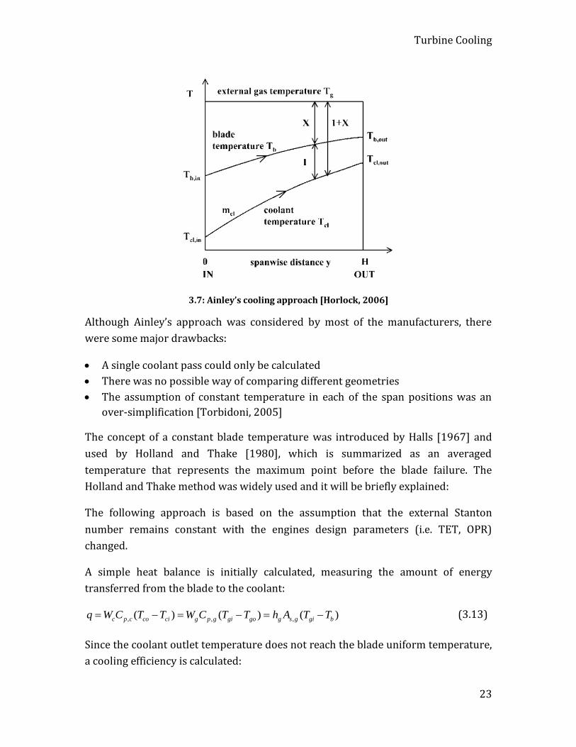
3.7: Ainley’s cooling approach [Horlock, 2006]
Although Ainley’s approach was considered by most of the manufacturers, there were some major drawbacks:
• A single coolant pass could only be calculated • There was no possible way of comparing different geometries • The assumption of constant temperature in each of the span positions was an
over-simplification [Torbidoni, 2005]
The concept of a constant blade temperature was introduced by Halls [1967] and used by Holland and Thake [1980], which is summarized as an averaged temperature that represents the maximum point before the blade failure. The Holland and Thake method was widely used and it will be briefly explained:
The following approach is based on the assumption that the external Stanton number remains constant with the engines design parameters (i.e. TET, OPR) changed.
A simple heat balance is initially calculated, measuring the amount of energy transferred from the blade to the coolant:
, , ,( ) ( ) ( )c p c co ci g p g gi go g s g gi bq W C T T W C T T h A T T= − = − = − (3.13)
Since the coolant outlet temperature does not reach the blade uniform temperature, a cooling efficiency is calculated:
Turbine Cooling
24
( ) / ( )c co ci b cin T T T T= − − (3.14)
Then it is assumed that in a family of similar gas turbines, the ratio of the area that heat transfer takes place to the cross-section of the main hot gas path is constant.
Those two concepts are introduced to the heat transfer calculation, along with the external Stanton number:
, , , , ,( / ) ( / )( / )( / )( ) / ( )c g s g x g p g p c g p g g g g i b c b ciW W A A C C h C V T T n T Tρ= − −
, , , ,( / )( / ) ( ) / ( )s g x g p g p c g gi b c b ciA A C C St T T n T T= − − (3.15)
This calculates the cooling mass flow rate as a fraction of the main gas flow rate
With further calculations, the following equation can be derived:
0 0/ (1 )Kξ ε ε= − (3.16)
It should be noted that /c gW Wξ = and that K is a constant that includes gas
properties, geometric ratios and the cooling efficiency. Finally, ε0 is the cooling effectiveness, defined as:
0 ( ) / ( )gi b gi ciT T T Tε = − − (3.17)
In a similar approach, film cooling is calculated by Holland and Thake [1980].
Considering the heat transfer taking place the following equation derives:
, , ,( ) ( )s g fc g aw b c p c co ciq A h T T W C T T= − = − (3.18)
Where hfc is the heat transfer coefficient for film cooling and Taw the adiabatic wall temperature.
The film cooling effectiveness can be defined as:
( ) / ( )fc g aw g coT T T Tε = − − (3.19)
And a ratio of the cooling mass flow to the main gas mass flow can be derived as previously, taking into account the Biot number and the TBC thickness and conductivity.

Turbine Cooling
25
The above mentioned method in practice needs a large number of inputs that may not be available in a preliminary stage and should be guessed. In addition it tends to underestimate the amount of the coolant mass flow compared to real designs, but this is normal as extra safety coefficients are introduced by the designers and some areas that may be introduced to the calculations are only cooled by convective cooling.
Horlock in 1973, in a similar way, developed a method that calculates the heat flow rate by convection per length unit of a “standard” turbine blade. According to Horlock, the external heat transfer rates are high near the leading edge, lower as the boundary layer thickens and high again after the transition point, where the presence of turbulence accelerates the process again.
Horlock uses an overall heat transfer relation developed by Ainley, based on the calculation of the mean Nusselt number for the gas part and based on assumptions for specific Reynolds number and cooling efficiency on the blade.
He then uses a model developed by Hodge [1960a], according to which the development of the thermal boundary layer is similar to the development of the momentum boundary layer, introducing proper corrections for the turbulent and laminar separation regions.
A combination then of the Nusselt-Reynolds-Prandtl relation and the semi-empirical laws developed by Hodge can express X with a number of geometrical and flow data. Among them, the coolant geometric parameter Z is introduced, as described by Ainley:
1.2
2/c cS AZl l
=
(3.20)
Where l is the blade chord length and Sc and Ac the total perimeter and area of the cooling passages.
A higher Z means a higher X and a higher ratio of the heat transferred to the coolant, compared to the heat transferred to the surface. According to Horlock, Some typical values of Z for an effective cooling lie between 150 and 250.
With the introduction of the Z parameter, a geometry input for the design of a cooling system has been achieved. With analysing the range of the inputs, the design of a specific cooling system can be determined.
Turbine Cooling
26
Consonni [1992] proposed a new model, based on Ainley’s work [1957]. In his approach, Consonni enabled the blade temperature variation in the radial direction and following the heat transfer calculations for the internal convective cooling, he determined the heat transfer coefficients and the technology factor Z. His improvements to the model include the introduction of TBC and of finite blade thickness. In addition, he includes the effects of film cooling with the following method:
Consonni considers the blade as a heat exchanger that includes both the blade itself and the film cooling flow. The external temperature is constant and equal to the gas temperature Tg for the case of a convectively cooled blade and to the adiabatic wall temperature Taw for the case of a film cooled blade. A new cooling efficiency is derived:
' ( ) / ( )c co ci g cin T T T T= − − (3.21)
Since the above equation is related to the known cooling efficiency definition, a coolant outlet temperature Tco can be determined. Then, by equating the heat flux between the two sides the blade outlet temperature can be calculated.
An iterative procedure can be then used, changing the geometry input parameters until the blade outlet temperature reaches the maximum allowable for the blade material. At this point, the minimum cooling flow rate can be determined, as a fraction of the total air mass flow.
Horlock [2006] and Torbidoni [2005] in their recent work identify the need for a higher resolution to the blade chord direction in the previous analysis. They follow Consonni’s work with introducing an elementary chord length and then integrating to the whole blade span.
Torbidoni and Massardo [2004a, 2004b] proposed a procedure for connecting an analytical blade cooling calculation model with a semi-empirical model. This idea combines the benefits and the accuracy of an analytical approach without the need for extensive geometry input data, since this would be difficult for the preliminary phase of a new design. This model, in addition, can evaluate the cooling performance of novel coolants, such as carbon dioxide or steam.
As discussed previously, the Z parameter represents the level technology of a cooling system and therefore can be the starting point of a new blade design,
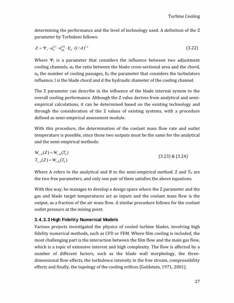
Turbine Cooling
27
determining the performance and the level of technology used. A definition of the Z parameter by Torbidoni follows:
0.2 0.8 1.2( / )i h pg hZ a n E l d= Ψ ⋅ ⋅ ⋅ ⋅ (3.22)
Where Ψi is a parameter that considers the influence between two adjustment cooling channels, αh the ratio between the blade cross-sectional area and the chord, np the number of cooling passages, Eh the parameter that considers the turbulators influence, l is the blade chord and d the hydraulic diameter of the cooling channel.
The Z parameter can describe in the influence of the blade internal system to the overall cooling performance. Although the Z value derives from analytical and semi-empirical calculations, it can be determined based on the existing technology and through the consideration of the Z values of existing systems, with a procedure defined as semi-empirical assessment module.
With this procedure, the determination of the coolant mass flow rate and outlet temperature is possible, since those two outputs must be the same for the analytical and the semi-empirical methods:
, ,
, ,
( ) ( )( ) ( )
c A c B b
c A c B b
W Z W TT Z W T
=
= (3.23) & (3.24)
Where A refers to the analytical and B to the semi-empirical method. Z and Tb are the two free parameters, and only one pair of them satisfies the above equations.
With this way, he manages to develop a design space where the Z parameter and the gas and blade target temperatures act as inputs and the coolant mass flow is the output, as a fraction of the air mass flow. A similar procedure follows for the coolant outlet pressure at the mixing point.
3.4.3.3 High Fidelity Numerical Models Various projects investigated the physics of cooled turbine blades, involving high fidelity numerical methods, such as CFD or FEM. Where film cooling is included, the most challenging part is the interaction between the film flow and the main gas flow, which is a topic of extensive interest and high complexity. The flow is affected by a number of different factors, such as the blade wall morphology, the three-dimensional flow effects, the turbulence intensity in the free stream, compressibility effects and finally, the topology of the cooling orifices [Goldstein, 1971, 2001].
Turbine Cooling
28
3.8: Garg’s [2000] turbine blade meshing
Garg [2000] investigated the performance of a three-dimensional film cooled turbine blade, illustrated in figure 3.8, by utilizing a NASA in-house Navier-Stokes solver. The blade, hub and shroud were calculated and a comparison with the same, un-cooled geometry was performed. Experimental results were also available to the author and the boundary conditions are based on them. Garg points out that even with the contemporary advanced tools that are available, the design of the cooling system is still based on one-dimensional analysis and empirical correlations, as the models analysed in previous sections. The verdict for every new design can only derive through experimental investigation of the setups, an expensive and time-consuming procedure. The numerical calculation specifications are discussed. The turbulence model used is the k-ω model of Wilcox [1994] with Menter's modifications [Menter, 1993] without any wall functions, since it was proved that gives better results in Garg’s previous works. As a requirement then, the target of a y+ lower than the unity was of high importance. The coolant mass flow rate was set by the actual blade. The results are presented in the form of the heat transfer coefficient h and film cooling effectiveness for all the regions of interest. The regions of extensive heat transfer rates are recognised and justified according to the coolant

Turbine Cooling
29
flow properties. A direct comparison between the cooled and un-cooled setups is performed as well.
NLR conducted a series of experiments and computational investigations and the results are presented in a series of papers by Tinga [2000, 2001] and de Wolf [2001]. The main purpose of this project is the life prediction of a F100-PW-220 low bypass turbofan military engine HP Turbine blade. The method included performance prediction tools (the in-house NLR GT performance code GSP), CFD and FEM analysis. The working fluid boundary conditions (i.e. Inlet and Outlet conditions) were given by the engine monitoring system. Two cases were considered, with and without film cooling, while the simplification of slot coolant injection rather than a number of cooling orifices was tested for simplicity in the CFD model.
The procedure started with entering the engine experimental and literature data to the performance analysis code. Various operating conditions were simulated, derived from the flight envelope. The boundary conditions were defined this way and uniformity was assumed for the turbine inlet. It should be pointed out that the number of the CFD cases that finally was simulated is lower than the actual ones for lower computational effort. The cases missing were calculated with the use of interpolation techniques. The external heat transfer, between the film and the gas is calculated through equation:
,( )ext ext fc g extq h T T= − (3.25)
Where it is assumed that the heat transfer coefficient hext can be derived from the un-cooled cases. The film temperature Tfc is determined by the film cooling efficiency. The local Stanton number is calculated as well. Concerning the specifications of the internal cooling system and the prediction of the coolant flow properties, an engineering model was used such as the ones presented earlier in this section. The distribution of the coolant mass flow to the various engine components was calculated analytically, with knowing the gas conditions and orifice areas.
The heat transfer and temperature predictions were treated as inputs to the FEM model that calculated the life, considering in addition the blade mechanical properties.
Lakehal [2001] presented a paper investigating the flow phenomena of film cooling in a more conceptual and microscopic way. They explore the effect of the
Turbine Cooling
30
coolant/gas mixing through an orifice near the leading edge of a symmetrical aerofoil. Two angles of injection are considered and a number of the k-ε turbulence model versions are tested, with the one proposed by Bergeles [1978] found to be the most accurate. Grid independency was also examined, with a number of different grids. The results are validated against experimental data of the same geometry and conditions, from experiments held in the Technical University of Darmstadt, Germany.
After running the model, the flow points of interest were identified, and the various flow zones were associated with the local rate of heat transfer. The film cooling effectiveness is the main output of the analysis and the way of comparing the measured with the calculated results.
Kegalj [2007] simulated the film cooling properties of the leading edge of a turbine stator blade using three-dimensional and one-dimensional methods, in order to compare it with a number of experiments they conducted as well. The overall aim was to investigate the accuracy of the numerical results and to assess if the one-dimensional method is sufficient for the design of a cooling system. The results show that the three-dimensional computational method can be very close to the experiment - using a carefully selected setup. On the other hand, the one-dimensional code can be close to the three-dimensional method and its use is recommended during the preliminary phase of blade design.
Collin [2004] investigated the aero/thermodynamics of three different actual blade designs, provided by a manufacturer. The objective of the investigation was to extract the detailed wall boundary conditions for a further FEM lifing analysis. The methodology includes an initial analysis of a blade with adiabatic domain boundaries and a second one with isothermal. The difference between the two cases reveals the heat transfer coefficient distribution. Following, details for the computational setup are presented by Collin. The control volume boundary conditions are given by the industrial partner, while validation against experimental data was performed for the mid-span region. A number of turbulence models were tried, with the v2-f to give the higher accuracy and a grid independence investigation was performed. The three dimensional flow properties were identified and the heat transfer in such regions was assessed with respect to the life properties. Two-dimensional simulations were performed as well, indicating that with no capturing of the three-dimensional effects, the heat transfer calculations may be invalid.
Turbine Cooling
31
Wheeler [2011] published their work on heat transfer taking place on a HP turbine blade tip. They used a CFD code validated by experimental data and they simulated two cases, the first with low and the second with high free stream speed. They analysed the total flow properties and local flow effects, along with the blade heat flux. They concluded that, as the separation bubble increases in size, the rest of the flow accelerates and the turbulent mixing decreases, affecting the local heat transfer coefficient.
Patil and Tafti [2013] focus again on the local geometry of a ribbed duct, in order to investigate the local heat transfer with the use of Large Eddy Simulation methods for two Reynolds numbers and validate the results against the experimental work of Rau [1998], Han [1986] and Tafti [2005]. The method used is wall-modelled LES setup, which was proved to predict the Nusselt number and friction factors in a good agreement with the experiments. Finally, the wall treatment proved to be essential for the flow prediction, in both velocity and thermal terms.
Duchaine [2009], demonstrated the coupling capabilities of a conjugate model that includes an LES flow solver and a heat transfer prediction method for a turbine blade. They validated the results and investigated the coupling stability. They concluded that this kind of simulations can be difficult to converge due to the complexity of three-dimensional flows, the diversity of physics that require different length and time scales and the extended size of computational requirements. On the other hand, LES is proved again to predict the flow in a good accuracy, in comparison to previous experiments on the same configuration.
32
4 Turbine Blade Heat Transfer Method
4.1 Introduction The method presented in this chapter is a computationally light numerical scheme, able to predict the heat transfer processes on a turbine blade or vane. The scheme is based on analytical and semi-empirical calculations for the blade, which is divided in a number of discrete elements, treated numerically.
The benefits from such an approach are numerous: The method is suitable for a detailed heat transfer analysis of any blade, in both span and chord, as being assembled by elements. This last gives the flexibility to simulate different geometries and configurations.
The method presented to this study differentiates in fidelity from any analytical method, since it can handle all forms of gas flow field boundary conditions, as it functions numerically, dividing the blade into a finite number of elements. It calculates the heat balance in every blade element and returns the local blade and coolant temperatures. It takes into account both convection and conduction terms in the used equations and offers a resolution from one-dimension, with a span analysis only, to two-dimensions, with span and chord analysis, to three-dimensions, with an additional thickness analysis. Of course, all three cases are referred to a three-dimensional blade and they differentiate in the directions the problem is allowed to proceed. The internal cooling geometry is represented by a single cooling channel with averaged heat transfer properties.
One-Dimensional Method
33
In contrast, the method is not as detailed as any CFD and FEM method, since the blade geometry used is a simplified form of a real configuration. Compared to any empirical methods, the method provides a higher resolution, based on a physics realistic solving process. It offers a quick assess of the cooling performance of a certain configuration, as the performance of the internal cooling system is averaged. This is the case for the film cooling modeling as well, where the local effects around the orifices are neglected. The approach followed by this method requires a minimum number of inputs and a small execution time, making the code suitable for optimisation studies as well, where a large number of individual cases can be considered and predicted. Overall, the method was designed to provide the inputs for two types of further analysis: First, a detailed investigation of the turbine performance, where the coolant state (i.e. total temperature and mass flow rate) the time it reenters the main cycle is needed for each blade row. Second, the conduction of three-dimensional estimation of the blade temperature field, suitable for mechanical integrity analyses, such as creep life estimation.
The structure of this work follows the method evolution from one-dimensional, discussing the differentiation from previous analytical and semi-empirical woks and the structure, and then passes to two-dimensions: A simple CFD study feeds the program with input data and further analysis on the structure and a number of features is performed. Finally, the third dimension is introduced, suitable for the modeling of multiple layers such as TBC, by utilizing an analysis based on Biot number.
4.2 One-Dimensional Method
4.2.1 Method Background The basis for this analysis is the work produced by Ainley [1957], Horlock [1973], Holland and Thake [1980], Consonni [1992] and most recently, Horlock and Torbidoni [2006].
Horlock and Torbidoni [2006], in their modeling produced analytical and semi-empirical mathematical relations able to predict the coolant and blade temperatures along the blade span of a simple model: The blade is treated as a heat exchanger between the external gas field and the internal coolant flow. Various options were examined, with constant or uniform blade and gas temperatures and the effects of TBC and film cooling included in some of them. The simplest form of equations, for uniform gas temperature is:
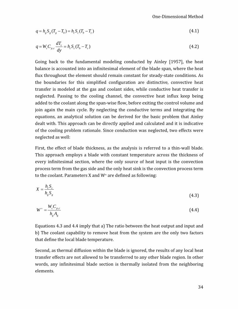
One-Dimensional Method
34
( ) ( )g g g b c c b cq h S T T h S T T= − = − (4.1)
, ( )cc p c c c b c
dTq W C h S T Tdy
= = − (4.2)
Going back to the fundamental modeling conducted by Ainley [1957], the heat balance is accounted into an infinitesimal element of the blade span, where the heat flux throughout the element should remain constant for steady-state conditions. As the boundaries for this simplified configuration are distinctive, convective heat transfer is modeled at the gas and coolant sides, while conductive heat transfer is neglected. Passing to the cooling channel, the convective heat influx keep being added to the coolant along the span-wise flow, before exiting the control volume and join again the main cycle. By neglecting the conductive terms and integrating the equations, an analytical solution can be derived for the basic problem that Ainley dealt with. This approach can be directly applied and calculated and it is indicative of the cooling problem rationale. Since conduction was neglected, two effects were neglected as well:
First, the effect of blade thickness, as the analysis is referred to a thin-wall blade. This approach employs a blade with constant temperature across the thickness of every infinitesimal section, where the only source of heat input is the convection process term from the gas side and the only heat sink is the convection process term to the coolant. Parameters X and W+ are defined as following:
c c
g g
h SXh S
= (4.3)
,c p c
g g
W CW
h A+ = (4.4)
Equations 4.3 and 4.4 imply that a) The ratio between the heat output and input and b) The coolant capability to remove heat from the system are the only two factors that define the local blade temperature.
Second, as thermal diffusion within the blade is ignored, the results of any local heat transfer effects are not allowed to be transferred to any other blade region. In other words, any infinitesimal blade section is thermally isolated from the neighboring elements.
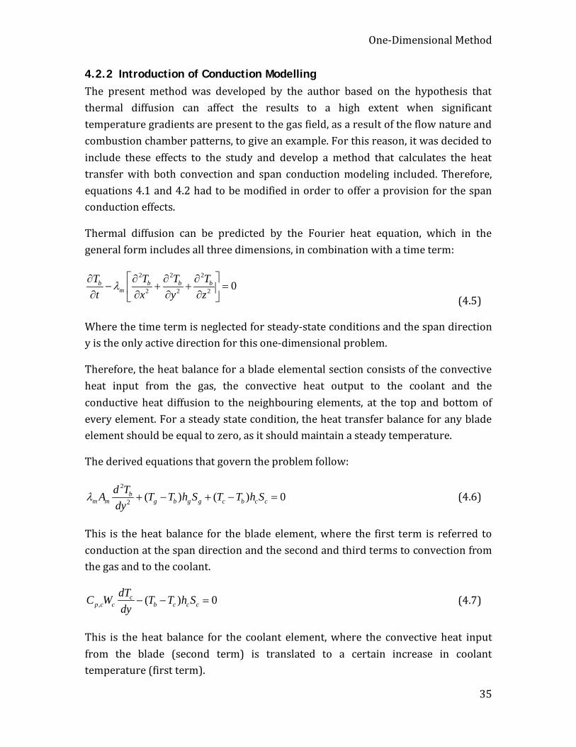
One-Dimensional Method
35
4.2.2 Introduction of Conduction Modelling The present method was developed by the author based on the hypothesis that thermal diffusion can affect the results to a high extent when significant temperature gradients are present to the gas field, as a result of the flow nature and combustion chamber patterns, to give an example. For this reason, it was decided to include these effects to the study and develop a method that calculates the heat transfer with both convection and span conduction modeling included. Therefore, equations 4.1 and 4.2 had to be modified in order to offer a provision for the span conduction effects.
Thermal diffusion can be predicted by the Fourier heat equation, which in the general form includes all three dimensions, in combination with a time term:
2 2 2
2 2 2 0b b b bm
T T T Tt x y z
λ ∂ ∂ ∂ ∂
− + + = ∂ ∂ ∂ ∂ (4.5)
Where the time term is neglected for steady-state conditions and the span direction y is the only active direction for this one-dimensional problem.
Therefore, the heat balance for a blade elemental section consists of the convective heat input from the gas, the convective heat output to the coolant and the conductive heat diffusion to the neighbouring elements, at the top and bottom of every element. For a steady state condition, the heat transfer balance for any blade element should be equal to zero, as it should maintain a steady temperature.
The derived equations that govern the problem follow:
2
2 ( ) ( ) 0bm m g b g g c b c c
d TA T T h S T T h Sdy
λ + − + − = (4.6)
This is the heat balance for the blade element, where the first term is referred to conduction at the span direction and the second and third terms to convection from the gas and to the coolant.
, ( ) 0cp c c b c c c
dTC W T T h Sdy
− − = (4.7)
This is the heat balance for the coolant element, where the convective heat input from the blade (second term) is translated to a certain increase in coolant temperature (first term).
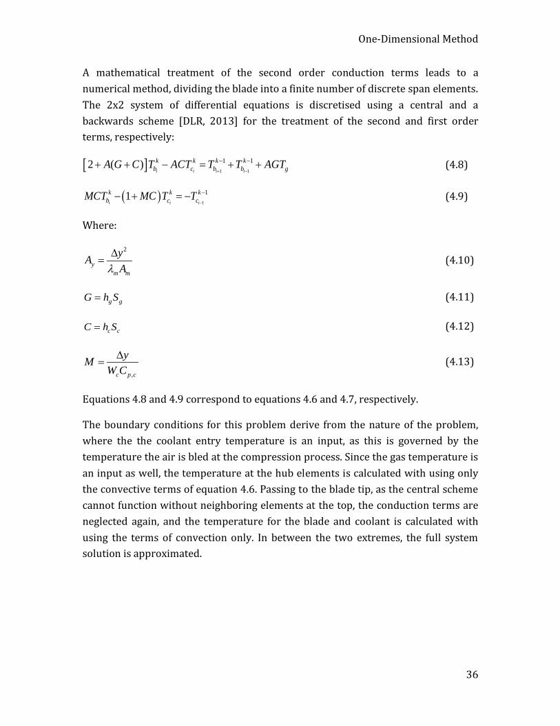
One-Dimensional Method
36
A mathematical treatment of the second order conduction terms leads to a numerical method, dividing the blade into a finite number of discrete span elements. The 2x2 system of differential equations is discretised using a central and a backwards scheme [DLR, 2013] for the treatment of the second and first order terms, respectively:
[ ]1 1
1 12 ( )i i i i
k k k kb c b b gA G C T ACT T T AGT
+ −
− −+ + − = + + (4.8)
( )1
11i i i
k k kb c cMCT MC T T
−
−− + = − (4.9)
Where:
2
ym m
yAAλ
∆= (4.10)
g gG h S= (4.11)
c cC h S= (4.12)
,c p c
yMW C∆
= (4.13)
Equations 4.8 and 4.9 correspond to equations 4.6 and 4.7, respectively.
The boundary conditions for this problem derive from the nature of the problem, where the the coolant entry temperature is an input, as this is governed by the temperature the air is bled at the compression process. Since the gas temperature is an input as well, the temperature at the hub elements is calculated with using only the convective terms of equation 4.6. Passing to the blade tip, as the central scheme cannot function without neighboring elements at the top, the conduction terms are neglected again, and the temperature for the blade and coolant is calculated with using the terms of convection only. In between the two extremes, the full system solution is approximated.
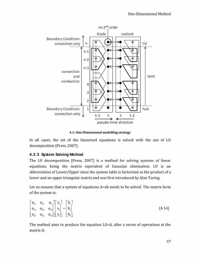
One-Dimensional Method
37
4.1: One-Dimensional modelling strategy
In all cases, the set of the linearised equations is solved with the use of LU decomposition [Press, 2007].
4.2.3 System Solving Method The LU decomposition [Press, 2007] is a method for solving systems of linear equations, being the matrix equivalent of Gaussian elimination. LU is an abbreviation of Lower/Upper since the system table is factorised as the product of a lower and an upper triangular matrix and was first introduced by Alan Turing.
Let us assume that a system of equations A=xb needs to be solved. The matrix form of the system is:
11 12 3 1 1
21 22 23 2 2
31 32 33 3 3
a a a x ba a a x ba a a x b
=
(4.14)
The method aims to produce the equation LU=A, after a series of operations at the matrix A:

One-Dimensional Method
38
11 11 12 3 11 12 3
21 22 22 23 21 22 23
31 32 33 33 31 32 33
0 00 0
0 0
l u u u a a al l u u a a al l l a a a a
=
(4.15)
The system is now transformed to the following expression:
11 11 12 3 1 1
21 22 22 23 2 2
31 32 33 33 3 3
0 00 0
0 0
l u u u x bl l u u x bl l l a x b
=
(4.16)
This above relation can be broken down into two individual equations:
Ly bLUx b
Ux y=
= ⇒ = (4.17)
Which eventually will give the values of matrix x, the solution to the initial system.
This process is followed for the solution of the system of equations for every element and every pseudo-time step at the method described in this chapter. The system of equations to be solved is 2x2, with the equations being 4.8 and 4.9:
11 12 1
21 22 2
b
c
Ta a bTa a b
=
The matrix elements can be calculated as:
[ ]11 2 ( )a A G C= + + (4.18)
12a AC= − (4.19)
21a MC= (4.20)
( )22 1a MC= − + (4.21)
1 1
1 11 i i
k kb b gb T T AGT+ −
− −= + + (4.22)
1
12 i
kcb T−
−= − (4.23)
With A, G, C, M as defined earlier, in equations 4.10 – 4.13.
One-Dimensional Method
39
It should be noted that the terms Tg and hg (included in G) may have a constant value for a constant gas temperature and heat transfer coefficient along the span, or they may vary for every element, being Tgi and hgi, if the gas temperature and heat transfer coefficient vary as well along the span. Both cases will be examined in the following paragraphs.
4.2.4 Internal Geometry Modelling As previously mentioned, the internal cooling network is modeled by a single channel with a constant heat transfer coefficient. That was a decision that simplifies any problem development to an extent acceptable for preliminary estimation of the cooling performance. Since the problem modeling is based on heat balance, this approach deals with the overall energy in a way that the total amount of enthalpy transferred is equal between the real geometry and the simplified one. The two parameters affecting the performance of the cooling system is the overall convective heat transfer coefficient between the blade and the coolant hc, and the coolant mass flow rate W. According to Horlock [1973], the cooling system technology level can be represented by parameter Z. Since the design aim for more efficient cooling systems is to enhance the amount of heat which is transferred from the blade to the coolant, this is expressed by the cooling efficiency:
co cic
b ci
T TnT T
−=
− (4.24)
Here, the exit coolant temperature Tco represents a higher exchange of heat for a given mass flow rate. Back in terms of modeling, the only factor in equation 4.6 governing the rate of heat transferred to the coolant for a given geometry is the mean heat transfer coefficient hc. Therefore, a higher level of technology implies a higher cooling efficiency and a better heat transfer coefficient hc.
Z technology parameter can be used for the determination of the mean internal flow heat transfer coefficient.
0.2 0.8 1.2( / )i h pg hZ a n E l d= Ψ ⋅ ⋅ ⋅ ⋅ (4.25)
Z parameter is proportional to the Number of Transfer Units and a linear function of the mean coolant heat transfer coefficient hc. The cooling efficiency nc is a function of the NTU, and since at the same time cooling efficiency nc is associated with the coolant outlet temperature, by adjusting the mean internal heat transfer coefficient,
One-Dimensional Method
40
the internal cooling performance of the blade is changing as well. Continuing, it can be assigned to a certain cooling efficiency, coolant outlet temperature and internal channel configuration, if the actual geometry is known.
Overall, the inputs required for this kind of analysis are the gas temperature Tg and heat transfer coefficient hg, which can be either constant or variable in the span direction. In addition, the coolant entry temperature Tc , mass flow rate W and mean heat transfer coefficient hc are required, along with a number of geometry data: The blade height H, the blade external and internal perimeters Sg and Sc and the area of conduction Am in the y-direction, equal to the metal areal in a blade cross-section. It is worth mentioning that the material conductivity is essential, as it governs the span thermal diffusion, according to equation 4.5.
4.2.5 Film Cooling Modelling Another addition to the method is the inclusion of a model that simulates the effects of film cooling. The film cooling model was introduced to to all three versions of the code, from one- to three-dimensional, as film cooling may be investigated in any degree of fidelity and in different kinds of problems.
First, film cooling effectiveness needs to be introduced:
g awfc
g co
T TT T
ε−
=− (4.26)
The idea behind the model is simple: As all calculations are performed with having an external gas field that transfers part of its heat to the blade, another layer could be introduced between the gas and the external surface of the blade that simulates the film.
The film consists of a mixture between the external gas and part of the coolant, which leaves the internal channel and is injected in a way that surrounds and protects the external blade surfaces. How effective is the mix, it is dictated by film cooling effectiveness: The closer the adiabatic wall temperature [Horlock, 2006] is to the coolant injection temperature, the more effective is the film cooling process, as the blade is subjected to a lower temperature. Therefore, effectiveness is an input to the method.
The code initially calculates the adiabatic wall temperature Taw with the use of the film effectiveness input, and mixes the calculated coolant temperature of the first

The Energy Efficient Engine – Method Inputs
41
run with the gas temperature at every span position. Therefore, the film temperature varies along the span, accordingly to the mix between the two components, as both the coolant and gas temperatures vary as well along the span.
At a second time, the blade is not surrounded anymore by the gas, and the external temperature differs significantly, as the film has been introduced. At this point, an iterative process is engaged, until the internal coolant and the film temperatures reach equilibrium.
Therefore, at the results an external gas temperature is reported, along with the adiabatic wall equilibrium temperature, the blade temperature and the coolant temperature at all span positions. It is important to mention at this point that in reality the film is not as uniform as modelled. There are certain locations on a blade that film cooling is used and the injection of coolant is handled by orifices of various specifications. Therefore it is normal for a significant non-uniformity to exist. But on the other hand, this method from the beginning does not focus again on any local flow properties, but only on the averaged film state for every span element row. The introduction of effectiveness as a way to assess the film cooling performance of a certain configuration leads towards this direction as well, as it is based on average and not local flow properties.
An important assumption of the method that should be mentioned is that no coolant mass flow is modelled to be lost along the cooling channel. All the mass that enters the blade at the hub, exits the blade at the tip, as previously.
4.3 The Energy Efficient Engine – Method Inputs The Energy Efficient Engine or E3 as called, is an early 1980s NASA concept for the development of a family of conceptual turbofan engines, assigned to General Electric and Pratt & Whitney. The overall aim was the development of an advanced for the era concept, that implements a number of contemporary design novelties. The project is very well documented [Gray, 1978] [Owens 1978] [NASA, 1980a] [NASA, 1980b] [NASA, 1982] [Davis, 1985] [Ciepluch, 1987] and detailed information for the high pressure turbine can be found at the relevant report [Thulin, 1982].
The Pratt & Whitney version of the high pressure turbine is used for all case studies at this chapter. The choice of this specific engine was made mainly due to the wide availability of data that the Energy Efficient Engine project offered. The choice between the Pratt & Whitney and the General Electric variant was made due to the

The Energy Efficient Engine – Method Inputs
42
single-stage design of the former, which helps the simulation and evaluation of the results.
Along the present chapter, a number of inputs were necessary for the function of the cooling prediction method and computer program. Table 4.1 summarises the data needed to be extracted from the report.
Table 4.1: One-Dimensional Essential Method Inputs
Stator and Rotor Blade span Blade external perimeter Total perimeter of cooling channels Average blade thickness Thermal Barrier Coating thickness Cross-section metal area Film Cooling effectiveness Coolant mass flow rate Coolant inlet temperature Gas heat transfer coefficient
Starting with the span, the dimensions of the vane and blade are illustrated at the meridional cross-section of the HPT in figure 4.2, and extracted from there.
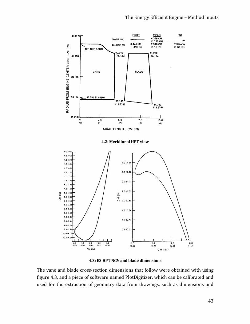
The Energy Efficient Engine – Method Inputs
43
4.2: Meridional HPT view
4.3: E3 HPT NGV and blade dimensions
The vane and blade cross-section dimensions that follow were obtained with using figure 4.3, and a piece of software named PlotDigitizer, which can be calibrated and used for the extraction of geometry data from drawings, such as dimensions and
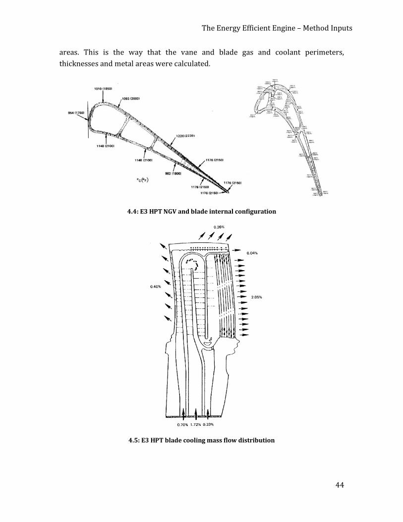
The Energy Efficient Engine – Method Inputs
44
areas. This is the way that the vane and blade gas and coolant perimeters, thicknesses and metal areas were calculated.
4.4: E3 HPT NGV and blade internal configuration
4.5: E3 HPT blade cooling mass flow distribution
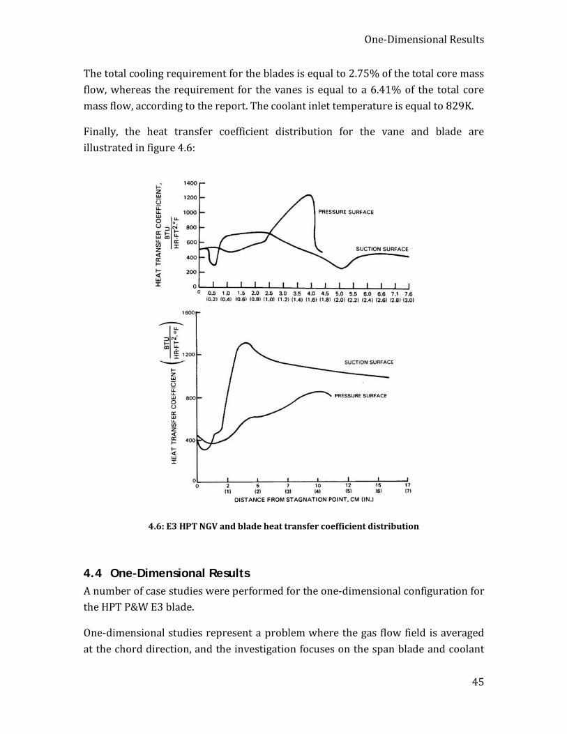
One-Dimensional Results
45
The total cooling requirement for the blades is equal to 2.75% of the total core mass flow, whereas the requirement for the vanes is equal to a 6.41% of the total core mass flow, according to the report. The coolant inlet temperature is equal to 829K.
Finally, the heat transfer coefficient distribution for the vane and blade are illustrated in figure 4.6:
4.6: E3 HPT NGV and blade heat transfer coefficient distribution
4.4 One-Dimensional Results A number of case studies were performed for the one-dimensional configuration for the HPT P&W E3 blade.
One-dimensional studies represent a problem where the gas flow field is averaged at the chord direction, and the investigation focuses on the span blade and coolant
One-Dimensional Results
46
temperature distribution. Therefore, the coolant is modelled to flow on a single channel at the span direction, from the root to the tip, where it exits the blade and mixes with the gas.
Of course, a number of approximations are included in such a scenario, with the main ones to be the constant gas temperature in the axial direction, a limitation that is going to be removed later, with the inclusion of chord heat transfer modelling. The single cooling channel is another assumption, as in modern blades the coolant follows a path that passes a blade multiple times, but that was necessary for a light design tool that requires a minimum amount of inputs.
The differentiation of this model compared to previous analytical ones is that the contribution of metal conduction along the span is accounted and demonstrated at the relevant section, influencing significantly the results.
For all simulations in the present paragraph, a base case was selected, with certain specifications. Then, some parametric analyses were performed with the range of the parameter indicated in every case individually.
The program inputs for the base case are the following:
Table 4.2: One-Dimensional Inputs for the rotor
One-Dimensional Inputs Blade span H=0.0608 m Blade external perimeter Sg=0.115 m Total perimeter of cooling channels Sc=0.0945 m Cross-section metal area Am=0.000145 m2 Blade conductivity λm=90 W/mK Coolant mass flow rate Wc=0.038 kg/s Coolant inlet temperature Tci=829 K
Gas heat transfer coefficient [averaged] hg=3423 W/m2K Coolant heat transfer coefficient [averaged] hc=2800 W/m2K
A parametric analysis for the level technology of the internal cooling geometry was performed, as illustrated in Figure 4.7. Three different cases were simulated, under a constant and uniform gas temperature and heat gas transfer coefficient along the span: A base case with a “standard” level of internal cooling technology and two different configurations with enhanced and reduced internal heat transfer
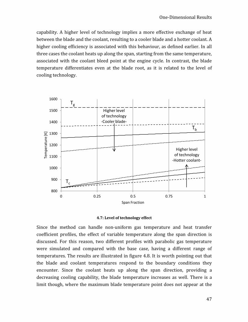
One-Dimensional Results
47
capability. A higher level of technology implies a more effective exchange of heat between the blade and the coolant, resulting to a cooler blade and a hotter coolant. A higher cooling efficiency is associated with this behaviour, as defined earlier. In all three cases the coolant heats up along the span, starting from the same temperature, associated with the coolant bleed point at the engine cycle. In contrast, the blade temperature differentiates even at the blade root, as it is related to the level of cooling technology.
4.7: Level of technology effect
Since the method can handle non-uniform gas temperature and heat transfer coefficient profiles, the effect of variable temperature along the span direction is discussed. For this reason, two different profiles with parabolic gas temperature were simulated and compared with the base case, having a different range of temperatures. The results are illustrated in figure 4.8. It is worth pointing out that the blade and coolant temperatures respond to the boundary conditions they encounter. Since the coolant heats up along the span direction, providing a decreasing cooling capability, the blade temperature increases as well. There is a limit though, where the maximum blade temperature point does not appear at the
800
900
1000
1100
1200
1300
1400
1500
1600
0 0.25 0.5 0.75 1
Tem
pera
ture
[K]
Span Fraction
Tg
Tb
Tc
Higher level of technology -Cooler blade-
Higher level of technology
-Hotter coolant-
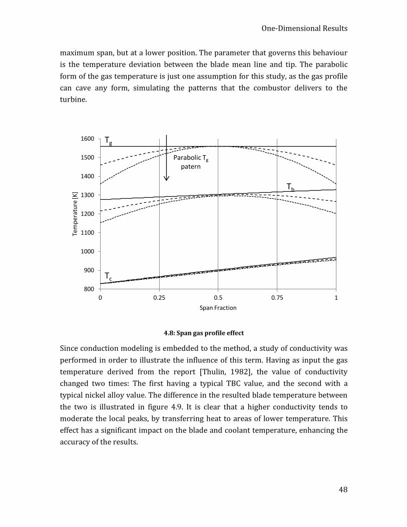
One-Dimensional Results
48
maximum span, but at a lower position. The parameter that governs this behaviour is the temperature deviation between the blade mean line and tip. The parabolic form of the gas temperature is just one assumption for this study, as the gas profile can cave any form, simulating the patterns that the combustor delivers to the turbine.
4.8: Span gas profile effect
Since conduction modeling is embedded to the method, a study of conductivity was performed in order to illustrate the influence of this term. Having as input the gas temperature derived from the report [Thulin, 1982], the value of conductivity changed two times: The first having a typical TBC value, and the second with a typical nickel alloy value. The difference in the resulted blade temperature between the two is illustrated in figure 4.9. It is clear that a higher conductivity tends to moderate the local peaks, by transferring heat to areas of lower temperature. This effect has a significant impact on the blade and coolant temperature, enhancing the accuracy of the results.
800
900
1000
1100
1200
1300
1400
1500
1600
0 0.25 0.5 0.75 1
Tem
pera
ture
[K]
Span Fraction
Parabolic Tg patern
Tg
Tb
Tc
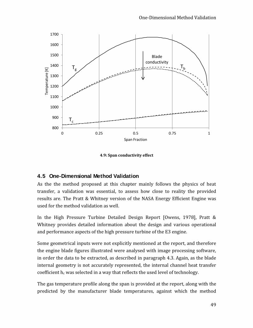
One-Dimensional Method Validation
49
4.9: Span conductivity effect
4.5 One-Dimensional Method Validation As the the method proposed at this chapter mainly follows the physics of heat transfer, a validation was essential, to assess how close to reality the provided results are. The Pratt & Whitney version of the NASA Energy Efficient Engine was used for the method validation as well.
In the High Pressure Turbine Detailed Design Report [Owens, 1978], Pratt & Whitney provides detailed information about the design and various operational and performance aspects of the high pressure turbine of the E3 engine.
Some geometrical inputs were not explicitly mentioned at the report, and therefore the engine blade figures illustrated were analysed with image processing software, in order the data to be extracted, as described in paragraph 4.3. Again, as the blade internal geometry is not accurately represented, the internal channel heat transfer coefficient hc was selected in a way that reflects the used level of technology.
The gas temperature profile along the span is provided at the report, along with the predicted by the manufacturer blade temperatures, against which the method
800
900
1000
1100
1200
1300
1400
1500
1600
1700
0 0.25 0.5 0.75 1
Tem
pera
ture
[K]
Span Fraction
Tg Tb
Tc
Blade conductivity
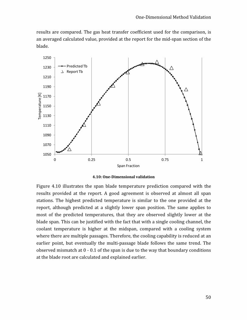
One-Dimensional Method Validation
50
results are compared. The gas heat transfer coefficient used for the comparison, is an averaged calculated value, provided at the report for the mid-span section of the blade.
4.10: One-Dimensional validation
Figure 4.10 illustrates the span blade temperature prediction compared with the results provided at the report. A good agreement is observed at almost all span stations. The highest predicted temperature is similar to the one provided at the report, although predicted at a slightly lower span position. The same applies to most of the predicted temperatures, that they are observed slightly lower at the blade span. This can be justified with the fact that with a single cooling channel, the coolant temperature is higher at the midspan, compared with a cooling system where there are multiple passages. Therefore, the cooling capability is reduced at an earlier point, but eventually the multi-passage blade follows the same trend. The observed mismatch at 0 - 0.1 of the span is due to the way that boundary conditions at the blade root are calculated and explained earlier.
1050
1070
1090
1110
1130
1150
1170
1190
1210
1230
1250
0 0.25 0.5 0.75 1
Tem
pera
ture
[K]
Span Fraction
Predicted Tb Report Tb

Two-Dimensional Method
51
4.6 Two-Dimensional Method The presented one-dimensional method provides a good first indication of the blade thermal behaviour, especially when gas temperature gradients exist at the span direction. As aforementioned, the temperature at the chord direction is averaged for both the gas and blade, so no resolution is provided along the gas expansion direction.
The introduction of the axial resolution may be challenging in terms of modelling and programming, and requires a more thorough problem setup from the user, but since the thermal processes taking place along the chord affect the results significantly, the extra effort is well justified.
If the method had been developed only to include convection modelling, the implementation would be relatively straightforward, as every blade element would be analysed independently and isolated from the four elements that it is directly neighbouring at this case. The thermal interaction of all the blade elements though, through heat transfer via conduction makes the method implementation more complex, as will be analysed at the next section.
The modelling of conduction though is justified, as the effects of conductivity are significant, not only in the span, but most importantly in the blade chord direction, where the flow field changes completely along the flow direction. Heat transfer modeling that includes only the convection terms means that any local flow property has a direct effect on the local blade area, without allowing it to be diffused. The blade responds directly to every spatial variation of the gas field, an assumption which can be simplistic. In reality, as heat diffuses isotropically, there is the tendency for temperature gradients to be moderated.
Mathematical modeling of the effects of conduction along the chord is a necessary development. The surrounding gas static temperature changes completely through the turbine and this should be captured by a cooling prediction method, justifying the introduction of a second dimension. Two main reasons for the static temperature variation along the chord follow: First, the flow acceleration through the NGV creates a significant drop in it. Second, as the total temperature drops through the rotor, the static temperature follows, having a steep negative gradient along the chord. These gradients should not be directly translated into a blade temperature profile, as energy is transferred within the material, resulting on a totally different pattern.

Two-Dimensional Method
52
Since the gas temperature Tg and heat transfer coefficient hg are inputs to the method, the stochastic nature of them means that each blade elementary area needs to be treated independently. Each element will have a different gas input. For this reason, the numerical strategy followed for the one-dimensional analysis is expanded to cover this two-dimensional problem: The blade is discretized into a finite number of elements in the span and chord directions, resulting to a further segmentation of the one-dimensional elements, that now offer a chord resolution as well.
The equations that describe the problem for the span direction derive from equations 4.6 and 4.7:
2
2 ( ) ( ) 0bm my g b g g c b c c
d TA T T h dx T T h dxdy
λ + − + − = (4.27)
, ( ) 0c cp c c c b c c
c
W dTC dx T T h dxS dy
− − = (4.28)
Two modifications were undertaken in order to accommodate the nature of the problem: First, the previously perimeter terms have become elementary lengths dxg and dxc, as they are now referred to a fraction of the blade and cooling channel perimeter, respectively. Second, the total mass flow through the cooling channel has been divided into flow elements along the span direction, the number of them being equal to the elements at the chord direction.
The linearised form of equations 4.27 and 4.28 follows:
, , , 1 , 1 ,
1 12 22 ( )
i j i j i j i j i j
k kk ky b y c b b y gA G C T A CT T T A GT
+ −
− − + + − = + + (4.29)
( ), , , 1
121
i j i j i j
kk kb c cMCT MC LT LT
−
−− + = − (4.30)
Where
2
ym my
yAAλ
∆=
(4.31)
g xgG h= ∆ (4.32)
Two-Dimensional Method
53
c xcC h= ∆ (4.33)
,c p c
yMW C∆
= (4.34)
c
c
xLS∆
= (4.35)
As this 2x2 system of equations promotes the problem to the span direction for a strip of elements, it needs to be iterated for all the element strips that form the blade perimeter. This loop promotes the heat diffusion for one pseudo-time step and only in the span direction. The next time step needs to promote the heat diffusion around the blade or, in other words, at the chord direction. The second pseudo-time step then, takes the results from the previous intermediate solution and calculates the heat diffusion circumferentially.
If this is scaled up, the odd pseudo-time steps promote the span diffusion, whereas the even steps the chord diffusion, alternating the direction of diffusion and moderating the temperature gradients according to the material conductivity.
For the chord direction then, equation 4.27 is modified to:
2
2 ( ) ( ) 0bm my g b g g c b c c
d TA T T h dx T T h dxdx
λ + − + − = (4.36)
With the linearised form being:
[ ], , 1, 1, ,
1 12 22 ( )
i j i j i j i j i j
k k k kx b x c b b x gA G C T A CT T T A GT
+ −
+ ++ + − = + + (4.37)
Where the elementary dimensions remain the same, as the elementary control volumes are the same as previously. On the other hand, the direction of the diffusion process has changed to peripheral-wise, or in other words from the y-axis to the x-axis.
The second equation of the system remains the same as 4.28, as it is referred to the progress of heat transfer to the coolant in a way that averaged properties are introduced.
, ( ) 0c cp c c c b c c
c
W dTC dx T T h dxS dy
− − =

Two-Dimensional Method
54
An interesting observation is that this scheme is necessary because of the thermal diffusion evolution in both axes. If conductivity had not been accounted, the solution to the problem would be again straightforward, since every element would be thermally isolated from the neighbouring ones. In such a case, the elementary blade and coolant temperatures would only be functions of the local gas temperature and heat transfer coefficients.
Figure 4.11 illustrates the modelling of a turbine blade on a schematic way:
4.11: Two-Dimensional turbine blade modelling
Schematically, the whole solving process is illustrated in figure 4.12.
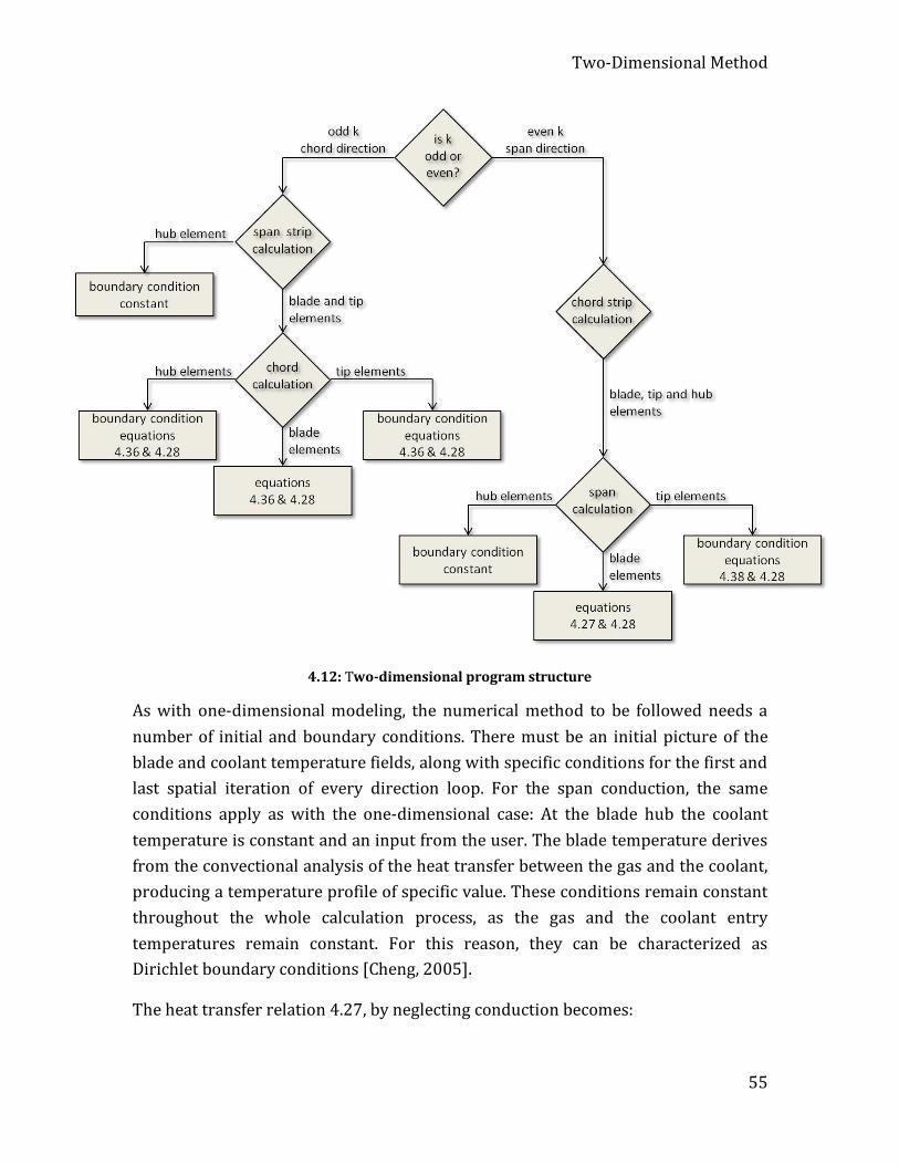
Two-Dimensional Method
55
4.12: Two-dimensional program structure
As with one-dimensional modeling, the numerical method to be followed needs a number of initial and boundary conditions. There must be an initial picture of the blade and coolant temperature fields, along with specific conditions for the first and last spatial iteration of every direction loop. For the span conduction, the same conditions apply as with the one-dimensional case: At the blade hub the coolant temperature is constant and an input from the user. The blade temperature derives from the convectional analysis of the heat transfer between the gas and the coolant, producing a temperature profile of specific value. These conditions remain constant throughout the whole calculation process, as the gas and the coolant entry temperatures remain constant. For this reason, they can be characterized as Dirichlet boundary conditions [Cheng, 2005].
The heat transfer relation 4.27, by neglecting conduction becomes:
Two-Dimensional Method
56
( ) ( ) 0g b g g c b c cT T h dx T T h dx− + − = (4.38)
Accompanied by known equation 4.28:
, ( ) 0c cp c c c b c c
c
W dTC dx T T h dxS dy
− − =
But since the gas and coolant temperatures remain constant throughout the whole blade calculation, the blade temperature remains constant as well, as described.
At the blade tip, the conduction modeling does not function without neighboring elements on top, so the code turns again into a convectional terms only equation, which follows:
( ) ( ) 0g b g g c b c cT T h dx T T h dx− + − =
With the linerised form being:
( ), ,,b i j i ji j
k kc gG C T CT GT+ − =
(4.39)
This time, the local coolant temperature is a variable and so is the tip blade temperature as well, which floats throughout the calculations until it converges to a certain value. Therefore, as the first derivative of the boundary conditions remains constant throughout the calculation they are boundary conditions of Neumann type [Cheng, 2005].
Passing to the chord direction, the same conditions apply for the hub and the tip. At this time step though, the code moves circumferentially, making a full circle around the blade chord direction elements. This means that a special condition should be introduced for the first and the last element of the loop. Specifically, the thermal diffusion should be directed to treat the edge elements as they interact thermally, to close the circle in other words, when moving peripherally. Therefore, they are characterized as periodic boundary conditions.
The required inputs for the two-dimensional analysis are the same with the one-dimensional, with two important differences: First, inputs are needed for the whole gas field around the blade. That means that gas temperature Tg and heat transfer coefficient hg are essential in all the elements as boundary conditions. Those inputs can be the outcome of a CFD analysis or an experiment.

Two-Dimensional Method
57
It is worth mentioning that since the gas flow field is formed by the blade and accounted as boundary condition, the external shape of the blade stops affecting the results of this method. Since the method is based on elementary heat balance, the local properties affect the rate of heat which is transferred to the coolant. A further remark on the modeling strategy is that the blade should have a constant external and internal perimeter in the span direction. It may be twisted span-wise though, as this will be accounted as boundary condition.
Overall, the method provides a calculation of the blade cooling requirements which is based on the heat being transferred or diffused, with the last being a modeling update for the engine conceptual design process. In addition, the results provided are of variable resolution in both span and chord directions, according to the user needs. Moreover, the span and chord discretisation can be selected independently. The suitable selection of this last parameter must be a compromise between the desired fidelity and the computational speed of the solving process. The method can be downgraded by setting the boundary conditions as constant along the desired direction. This makes the problem simpler, as there are not always input data available for the totality of the flow field.
Passing to the results, there are two kinds of output data. First the data needed for engine performance prediction: The coolant mass flow rate and temperature at the blade exit are essential figures for the accurate prediction of one-dimensional turbines and the overall engine performance, at a larger scale, as discussed at the following chapter. Since a turbine blade row can be simulated independently, the prediction of the gas state and the gradual mixing with the individual cooling flows can be performed [Kurzke, 2002]. It is worth mentioning that the method is suitable for both stators and rotors, as the main difference between the two are the gas boundary conditions. Second, the blade temperature at all span and chord locations is calculated by the method, an essential input for preliminary creep analysis.
There are some limitations as well that the method does not address. First, detailed picture of the gas flow field is required, i.e. gas temperature and heat transfer coefficient. That information is usually more difficult to obtain compared to averaged values at different engine stations. Second, the internal cooling system is not modeled in detail, having a single cooling channel with an averaged heat transfer coefficient. The result of this is a metal temperature that is just indicative of the reality and not predicted in detail. On the other hand, a detailed representation
Turbine Blade CFD Analysis
58
of the actual geometry would be extremely challenging and long, a process not suitable for a preliminary investigation.
Although the method is based on existing analytical and semi-empirical schemes, it follows a numerical approach. This approach is more demanding computationally and potentially numerically sensitive, but includes modeling of conduction in two directions, an important detail of turbine operation. It introduces a numerical error as well, by neglecting the high order Taylor series terms during the equations discretization. On the other hand, it provides the flexibility to solve the cooling problem of the most common configurations, with variable gas flow field topology.
As previously mentioned, the method requires the surrounding gas state as input, i.e. the gas temperature and heat transfer coefficient for every blade element. Uniform gas inputs are an option as well in any of the two directions, reducing the resolution by one dimension in the case of uniform chord gas state. If the span gas temperature and coefficient profile remain constant along the span, this results again to a variable blade and coolant temperature at the span direction, as the coolant heats up and provides reduced cooling capability towards this direction.
4.7 Turbine Blade CFD Analysis As mentioned, the surrounding gas state can be derived from a number of different sources, such as experiments, or numerical flow prediction methods, including CFD. For the scopes of this work, a turbine stage CFD analysis was performed, in order to provide the method with the necessary boundary conditions.
As the availability of detailed information on the design and performance of gas turbine engines is limited in general, the geometry of the high pressure turbine of the Pratt & Whitney Energy Efficient Engine was selected, mainly due to the extended availability of data .
The geometry of the model includes the whole single-stage HPT with the simplification of no rotor tip modelling. Therefore, no tip leakages were investigated.
The overall model configuration is illustrated in figure 4.13.
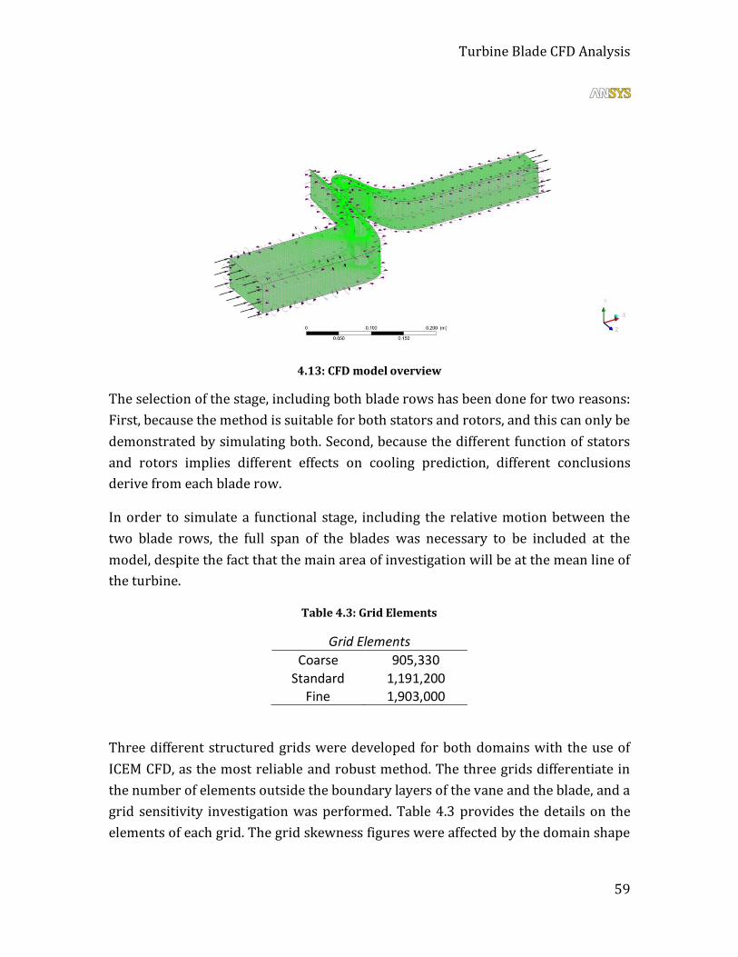
Turbine Blade CFD Analysis
59
4.13: CFD model overview
The selection of the stage, including both blade rows has been done for two reasons: First, because the method is suitable for both stators and rotors, and this can only be demonstrated by simulating both. Second, because the different function of stators and rotors implies different effects on cooling prediction, different conclusions derive from each blade row.
In order to simulate a functional stage, including the relative motion between the two blade rows, the full span of the blades was necessary to be included at the model, despite the fact that the main area of investigation will be at the mean line of the turbine.
Table 4.3: Grid Elements
Grid Elements Coarse 905,330
Standard 1,191,200 Fine 1,903,000
Three different structured grids were developed for both domains with the use of ICEM CFD, as the most reliable and robust method. The three grids differentiate in the number of elements outside the boundary layers of the vane and the blade, and a grid sensitivity investigation was performed. Table 4.3 provides the details on the elements of each grid. The grid skewness figures were affected by the domain shape
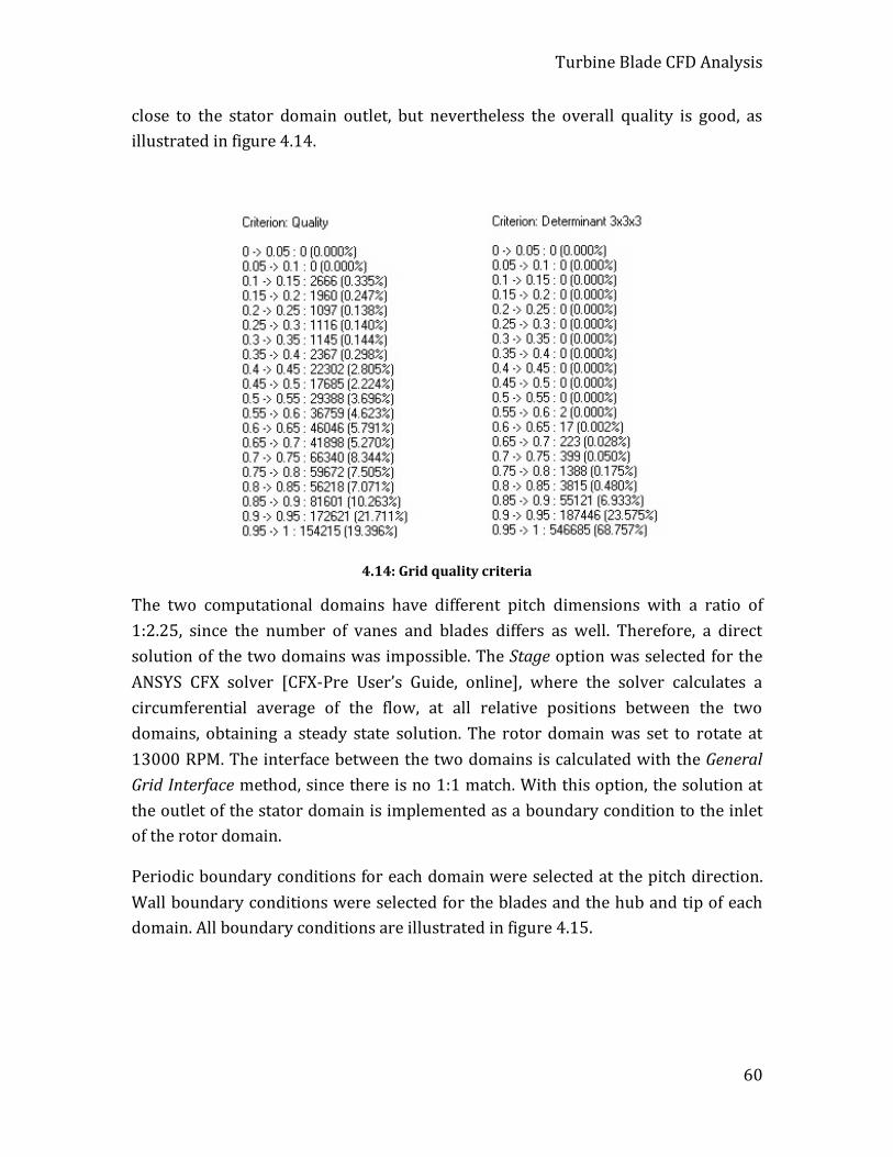
Turbine Blade CFD Analysis
60
close to the stator domain outlet, but nevertheless the overall quality is good, as illustrated in figure 4.14.
4.14: Grid quality criteria
The two computational domains have different pitch dimensions with a ratio of 1:2.25, since the number of vanes and blades differs as well. Therefore, a direct solution of the two domains was impossible. The Stage option was selected for the ANSYS CFX solver [CFX-Pre User’s Guide, online], where the solver calculates a circumferential average of the flow, at all relative positions between the two domains, obtaining a steady state solution. The rotor domain was set to rotate at 13000 RPM. The interface between the two domains is calculated with the General Grid Interface method, since there is no 1:1 match. With this option, the solution at the outlet of the stator domain is implemented as a boundary condition to the inlet of the rotor domain.
Periodic boundary conditions for each domain were selected at the pitch direction. Wall boundary conditions were selected for the blades and the hub and tip of each domain. All boundary conditions are illustrated in figure 4.15.
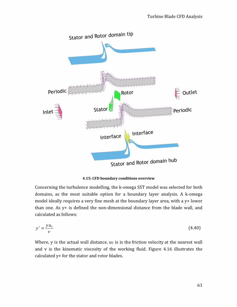
Turbine Blade CFD Analysis
61
4.15: CFD boundary conditions overview
Concerning the turbulence modelling, the k-omega SST model was selected for both domains, as the most suitable option for a boundary layer analysis. A k-omega model ideally requires a very fine mesh at the boundary layer area, with a y+ lower than one. As y+ is defined the non-dimensional distance from the blade wall, and calculated as follows:
Ty uyν
+ ≡ (4.40)
Where, y is the actual wall distance, uT is is the friction velocity at the nearest wall and v is the kinematic viscosity of the working fluid. Figure 4.16 illustrates the calculated y+ for the stator and rotor blades.

Turbine Blade CFD Analysis
62
4.16: Vane and blade y+ distribution
A grid sensitivity analysis was performed for the three different models, in order to evaluate the dependency on truncation error [Stoer, 2002]. Figures 4.17 and 4.18 illustrate the differences among the models as concerning the gas static temperature Tg at the stator and rotor.
4.17: Stator gas static temperature, Grid sensitivity
1300
1350
1400
1450
1500
1550
1600
1650
1700
0 0.25 0.5 0.75 1
Gas
tem
pera
ture
[K]
Fraction of Perimeter
Coarse grid Standard grid Fine grid
Trailing edge
Pressure side
Suction side
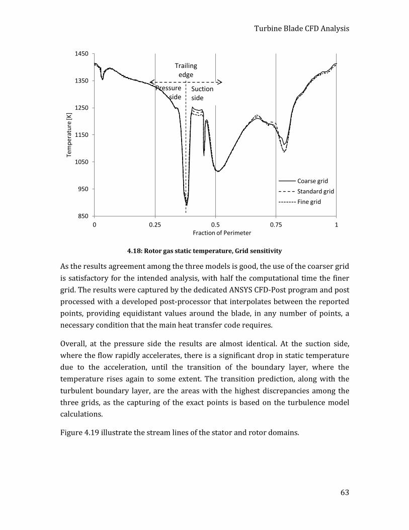
Turbine Blade CFD Analysis
63
4.18: Rotor gas static temperature, Grid sensitivity
As the results agreement among the three models is good, the use of the coarser grid is satisfactory for the intended analysis, with half the computational time the finer grid. The results were captured by the dedicated ANSYS CFD-Post program and post processed with a developed post-processor that interpolates between the reported points, providing equidistant values around the blade, in any number of points, a necessary condition that the main heat transfer code requires.
Overall, at the pressure side the results are almost identical. At the suction side, where the flow rapidly accelerates, there is a significant drop in static temperature due to the acceleration, until the transition of the boundary layer, where the temperature rises again to some extent. The transition prediction, along with the turbulent boundary layer, are the areas with the highest discrepancies among the three grids, as the capturing of the exact points is based on the turbulence model calculations.
Figure 4.19 illustrate the stream lines of the stator and rotor domains.
850
950
1050
1150
1250
1350
1450
0 0.25 0.5 0.75 1
Tem
pera
ture
[K]
Fraction of Perimeter
Coarse grid Standard grid Fine grid
Trailing edge
Pressure side
Suction side
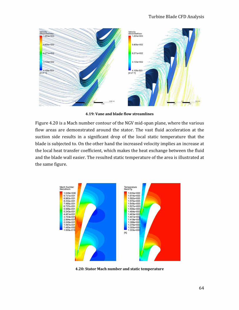
Turbine Blade CFD Analysis
64
4.19: Vane and blade flow streamlines
Figure 4.20 is a Mach number contour of the NGV mid-span plane, where the various flow areas are demonstrated around the stator. The vast fluid acceleration at the suction side results in a significant drop of the local static temperature that the blade is subjected to. On the other hand the increased velocity implies an increase at the local heat transfer coefficient, which makes the heat exchange between the fluid and the blade wall easier. The resulted static temperature of the area is illustrated at the same figure.
4.20: Stator Mach number and static temperature
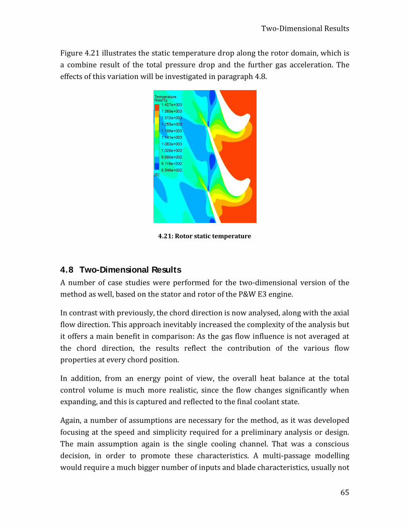
Two-Dimensional Results
65
Figure 4.21 illustrates the static temperature drop along the rotor domain, which is a combine result of the total pressure drop and the further gas acceleration. The effects of this variation will be investigated in paragraph 4.8.
4.21: Rotor static temperature
4.8 Two-Dimensional Results A number of case studies were performed for the two-dimensional version of the method as well, based on the stator and rotor of the P&W E3 engine.
In contrast with previously, the chord direction is now analysed, along with the axial flow direction. This approach inevitably increased the complexity of the analysis but it offers a main benefit in comparison: As the gas flow influence is not averaged at the chord direction, the results reflect the contribution of the various flow properties at every chord position.
In addition, from an energy point of view, the overall heat balance at the total control volume is much more realistic, since the flow changes significantly when expanding, and this is captured and reflected to the final coolant state.
Again, a number of assumptions are necessary for the method, as it was developed focusing at the speed and simplicity required for a preliminary analysis or design. The main assumption again is the single cooling channel. That was a conscious decision, in order to promote these characteristics. A multi-passage modelling would require a much bigger number of inputs and blade characteristics, usually not
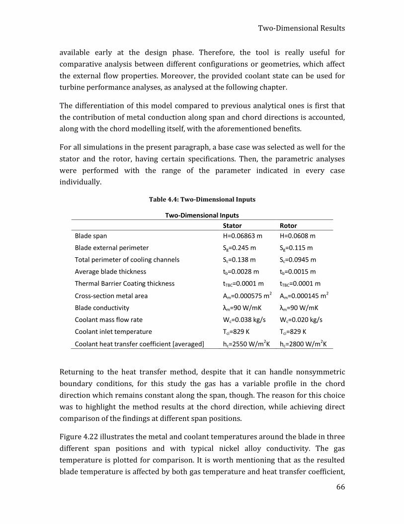
Two-Dimensional Results
66
available early at the design phase. Therefore, the tool is really useful for comparative analysis between different configurations or geometries, which affect the external flow properties. Moreover, the provided coolant state can be used for turbine performance analyses, as analysed at the following chapter.
The differentiation of this model compared to previous analytical ones is first that the contribution of metal conduction along span and chord directions is accounted, along with the chord modelling itself, with the aforementioned benefits.
For all simulations in the present paragraph, a base case was selected as well for the stator and the rotor, having certain specifications. Then, the parametric analyses were performed with the range of the parameter indicated in every case individually.
Table 4.4: Two-Dimensional Inputs
Two-Dimensional Inputs Stator Rotor Blade span H=0.06863 m H=0.0608 m Blade external perimeter Sg=0.245 m Sg=0.115 m Total perimeter of cooling channels Sc=0.138 m Sc=0.0945 m Average blade thickness tb=0.0028 m tb=0.0015 m Thermal Barrier Coating thickness tTBC=0.0001 m tTBC=0.0001 m Cross-section metal area Am=0.000575 m2 Am=0.000145 m2 Blade conductivity λm=90 W/mK λm=90 W/mK Coolant mass flow rate Wc=0.038 kg/s Wc=0.020 kg/s Coolant inlet temperature Tci=829 K Tci=829 K Coolant heat transfer coefficient [averaged] hc=2550 W/m2K hc=2800 W/m2K
Returning to the heat transfer method, despite that it can handle nonsymmetric boundary conditions, for this study the gas has a variable profile in the chord direction which remains constant along the span, though. The reason for this choice was to highlight the method results at the chord direction, while achieving direct comparison of the findings at different span positions.
Figure 4.22 illustrates the metal and coolant temperatures around the blade in three different span positions and with typical nickel alloy conductivity. The gas temperature is plotted for comparison. It is worth mentioning that as the resulted blade temperature is affected by both gas temperature and heat transfer coefficient,
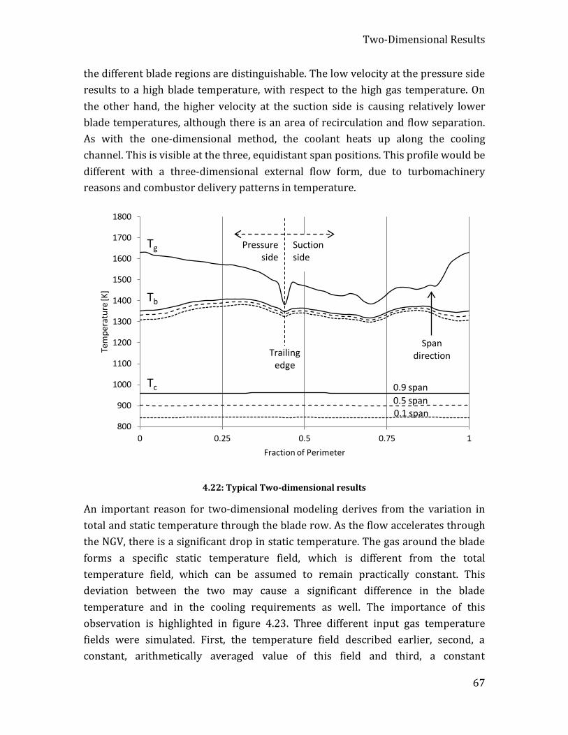
Two-Dimensional Results
67
the different blade regions are distinguishable. The low velocity at the pressure side results to a high blade temperature, with respect to the high gas temperature. On the other hand, the higher velocity at the suction side is causing relatively lower blade temperatures, although there is an area of recirculation and flow separation. As with the one-dimensional method, the coolant heats up along the cooling channel. This is visible at the three, equidistant span positions. This profile would be different with a three-dimensional external flow form, due to turbomachinery reasons and combustor delivery patterns in temperature.
4.22: Typical Two-dimensional results
An important reason for two-dimensional modeling derives from the variation in total and static temperature through the blade row. As the flow accelerates through the NGV, there is a significant drop in static temperature. The gas around the blade forms a specific static temperature field, which is different from the total temperature field, which can be assumed to remain practically constant. This deviation between the two may cause a significant difference in the blade temperature and in the cooling requirements as well. The importance of this observation is highlighted in figure 4.23. Three different input gas temperature fields were simulated. First, the temperature field described earlier, second, a constant, arithmetically averaged value of this field and third, a constant
800
900
1000
1100
1200
1300
1400
1500
1600
1700
1800
0 0.25 0.5 0.75 1
Tem
pera
ture
[K]
Fraction of Perimeter
Trailing edge
Pressure side
Suction side
Tg
Tb
Tc 0.9 span
0.5 span 0.1 span
Span direction
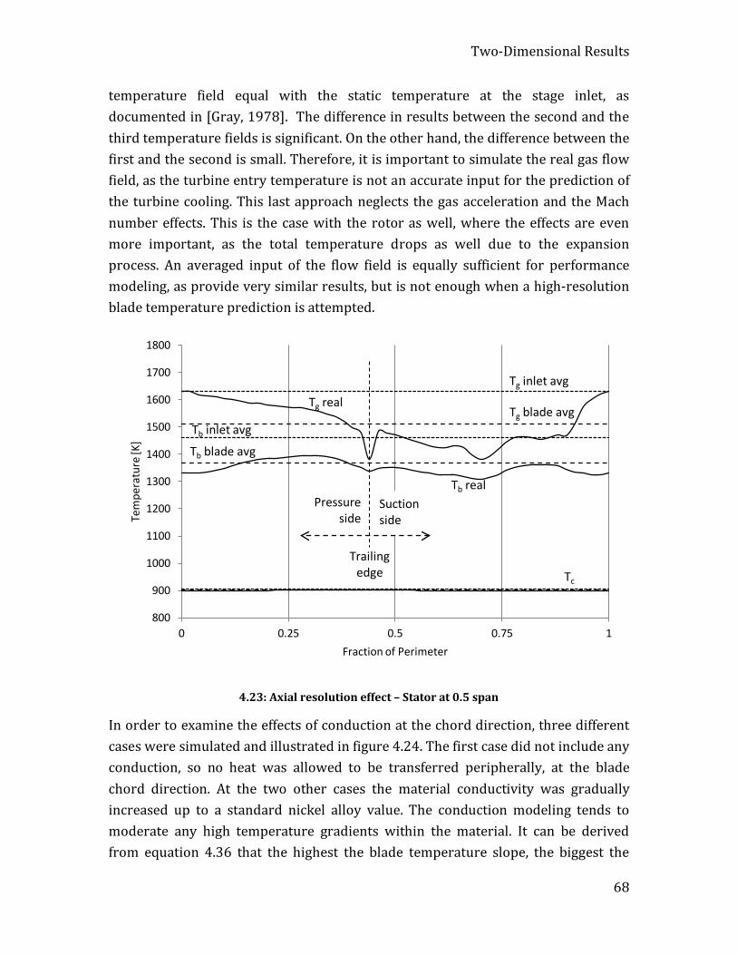
Two-Dimensional Results
68
temperature field equal with the static temperature at the stage inlet, as documented in [Gray, 1978]. The difference in results between the second and the third temperature fields is significant. On the other hand, the difference between the first and the second is small. Therefore, it is important to simulate the real gas flow field, as the turbine entry temperature is not an accurate input for the prediction of the turbine cooling. This last approach neglects the gas acceleration and the Mach number effects. This is the case with the rotor as well, where the effects are even more important, as the total temperature drops as well due to the expansion process. An averaged input of the flow field is equally sufficient for performance modeling, as provide very similar results, but is not enough when a high-resolution blade temperature prediction is attempted.
4.23: Axial resolution effect – Stator at 0.5 span
In order to examine the effects of conduction at the chord direction, three different cases were simulated and illustrated in figure 4.24. The first case did not include any conduction, so no heat was allowed to be transferred peripherally, at the blade chord direction. At the two other cases the material conductivity was gradually increased up to a standard nickel alloy value. The conduction modeling tends to moderate any high temperature gradients within the material. It can be derived from equation 4.36 that the highest the blade temperature slope, the biggest the
800
900
1000
1100
1200
1300
1400
1500
1600
1700
1800
0 0.25 0.5 0.75 1
Tem
pera
ture
[K]
Fraction of Perimeter
Trailing edge
Pressure side
Suction side
Tg inlet avg
Tg blade avg Tg real
Tb blade avg
Tb inlet avg
Tb real
Tc
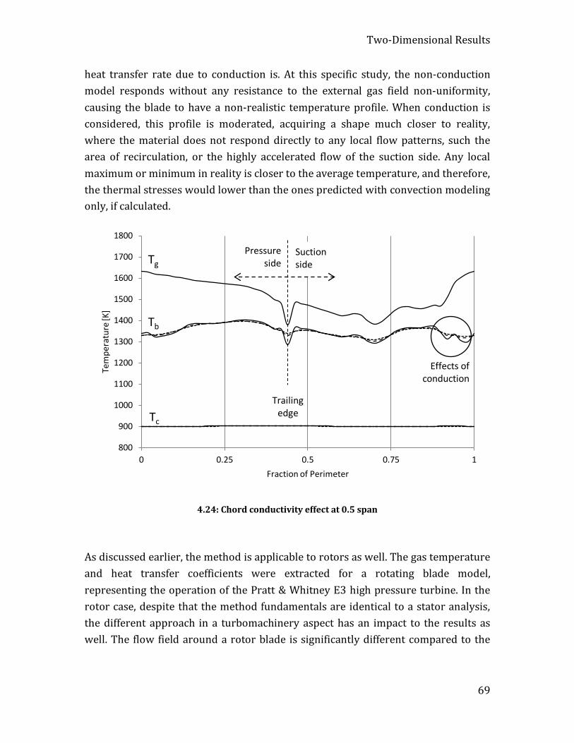
Two-Dimensional Results
69
heat transfer rate due to conduction is. At this specific study, the non-conduction model responds without any resistance to the external gas field non-uniformity, causing the blade to have a non-realistic temperature profile. When conduction is considered, this profile is moderated, acquiring a shape much closer to reality, where the material does not respond directly to any local flow patterns, such the area of recirculation, or the highly accelerated flow of the suction side. Any local maximum or minimum in reality is closer to the average temperature, and therefore, the thermal stresses would lower than the ones predicted with convection modeling only, if calculated.
4.24: Chord conductivity effect at 0.5 span
As discussed earlier, the method is applicable to rotors as well. The gas temperature and heat transfer coefficients were extracted for a rotating blade model, representing the operation of the Pratt & Whitney E3 high pressure turbine. In the rotor case, despite that the method fundamentals are identical to a stator analysis, the different approach in a turbomachinery aspect has an impact to the results as well. The flow field around a rotor blade is significantly different compared to the
800
900
1000
1100
1200
1300
1400
1500
1600
1700
1800
0 0.25 0.5 0.75 1
Tem
pera
ture
[K]
Fraction of Perimeter
Trailing edge
Pressure side
Suction side Tg
Tb
Tc
Effects of conduction

Two-Dimensional Results
70
one around the stator, mainly because of the motion and the different total pressure field.
At the stator, the gas acceleration results to a static pressure drop that has impact on the temperature that the surface experiences. In the rotor case, this effect still exists, since there is a further gas acceleration at the stationary plane, but the total temperature drop due to the expansion results has a combined effect on that.
Figure 4.25, illustrates the results of this analysis, where the aforementioned effects are visible. The gas static temperature drops vastly from leading edge to the trailing edge, while having some variations at the suction side, mainly due to the boundary layer transition. This results on an equivalent variation at the blade temperature that follows the general trend. This variation has a great impact on the thermal stresses within the blade and needs to be accounted at the design.
4.25: Axial resolution effect – Rotor at 0.5 span
At the same chart, two other averaging scenarios are investigated. The first scenario investigates the case where the rotor inlet gas temperature is used as an input for
800
900
1000
1100
1200
1300
1400
1500
0 0.25 0.5 0.75 1
Tem
pera
ture
[K]
Fraction of Perimeter
Trailing edge
Pressure side
Suction side
Tg inlet avg
Tg blade avg
Tg real
Tb blade avg
Tb inlet avg
Tb real
Tc
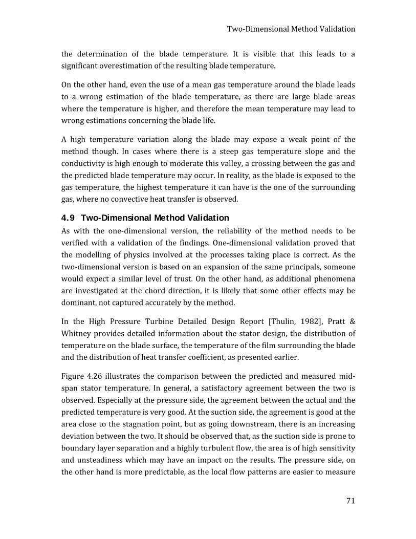
Two-Dimensional Method Validation
71
the determination of the blade temperature. It is visible that this leads to a significant overestimation of the resulting blade temperature.
On the other hand, even the use of a mean gas temperature around the blade leads to a wrong estimation of the blade temperature, as there are large blade areas where the temperature is higher, and therefore the mean temperature may lead to wrong estimations concerning the blade life.
A high temperature variation along the blade may expose a weak point of the method though. In cases where there is a steep gas temperature slope and the conductivity is high enough to moderate this valley, a crossing between the gas and the predicted blade temperature may occur. In reality, as the blade is exposed to the gas temperature, the highest temperature it can have is the one of the surrounding gas, where no convective heat transfer is observed.
4.9 Two-Dimensional Method Validation As with the one-dimensional version, the reliability of the method needs to be verified with a validation of the findings. One-dimensional validation proved that the modelling of physics involved at the processes taking place is correct. As the two-dimensional version is based on an expansion of the same principals, someone would expect a similar level of trust. On the other hand, as additional phenomena are investigated at the chord direction, it is likely that some other effects may be dominant, not captured accurately by the method.
In the High Pressure Turbine Detailed Design Report [Thulin, 1982], Pratt & Whitney provides detailed information about the stator design, the distribution of temperature on the blade surface, the temperature of the film surrounding the blade and the distribution of heat transfer coefficient, as presented earlier.
Figure 4.26 illustrates the comparison between the predicted and measured mid-span stator temperature. In general, a satisfactory agreement between the two is observed. Especially at the pressure side, the agreement between the actual and the predicted temperature is very good. At the suction side, the agreement is good at the area close to the stagnation point, but as going downstream, there is an increasing deviation between the two. It should be observed that, as the suction side is prone to boundary layer separation and a highly turbulent flow, the area is of high sensitivity and unsteadiness which may have an impact on the results. The pressure side, on the other hand is more predictable, as the local flow patterns are easier to measure
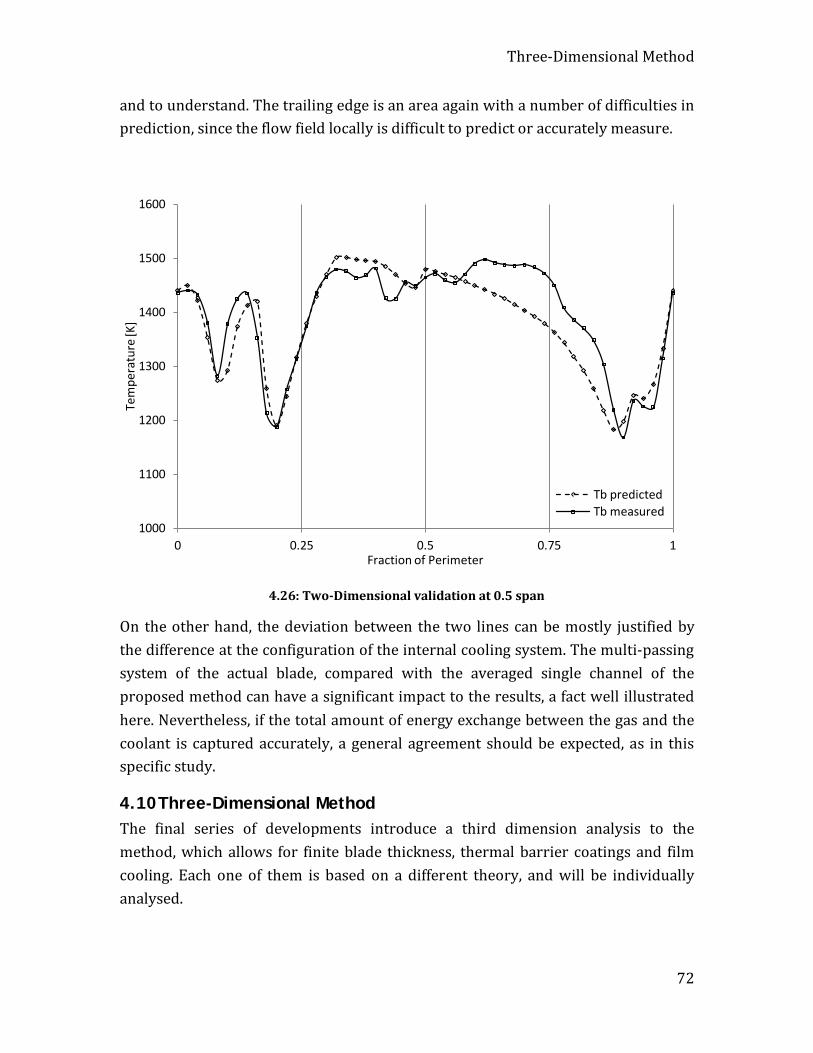
Three-Dimensional Method
72
and to understand. The trailing edge is an area again with a number of difficulties in prediction, since the flow field locally is difficult to predict or accurately measure.
4.26: Two-Dimensional validation at 0.5 span
On the other hand, the deviation between the two lines can be mostly justified by the difference at the configuration of the internal cooling system. The multi-passing system of the actual blade, compared with the averaged single channel of the proposed method can have a significant impact to the results, a fact well illustrated here. Nevertheless, if the total amount of energy exchange between the gas and the coolant is captured accurately, a general agreement should be expected, as in this specific study.
4.10 Three-Dimensional Method The final series of developments introduce a third dimension analysis to the method, which allows for finite blade thickness, thermal barrier coatings and film cooling. Each one of them is based on a different theory, and will be individually analysed.
1000
1100
1200
1300
1400
1500
1600
0 0.25 0.5 0.75 1
Tem
pera
ture
[K]
Fraction of Perimeter
Tb predicted Tb measured
Three-Dimensional Method
73
The one- and two-dimensional models presented so far are capable of simulating the thermal diffusion that allows the heat to be transferred at the whole of the blade surface, but do not have any provision for modeling the heat transferred across the blade thickness. As previously explained, the blade was still considered to be thin-walled, an assumption that gives to every element a single temperature value. In reality, one one or more material layers give a certain temperature profile to the blade wall, which should be modeled as well, providing a third dimension to the results. Therefore, the last development was to include provision for the evolution of the problem to the third dimension of the blade model as well. The additional dimension implies a finite blade thickness, which can be primarily used for TBC modeling. This feature has again a fundamental influence to both the performance of a cooled turbine blade and the mechanical integrity of it.
According to Henze [2013], the Biot number of a turbine blade indicates the order of magnitude between the external convection and the conduction within the blade material. The models of the previous sections are developed in a form where material conduction counts for heat diffusion in the span and peripheral directions, but since the blade is considered to have a uniform temperature across the thickness direction, the resolution was up to two-dimensional. This means that by adjusting the material conductivity the local temperature peaks and valleys on the blade surface are accordingly adjusted, as heat is allowed to be transferred, but the mean levels of blade and coolant temperatures remain the same, as there is no provision for modeling of the heat diffusion in the third direction. In reality, temperature forms a gradient from the blade external surface to the internal one, adjacent to coolant.
An additional feature was developed to take into consideration the finite thickness of an actual blade, along with the effects of TBC and the temperature gradients associated with the two. The approach can be divided into two discrete phases: First, an identical type of analysis with the two-dimensional method is performed, having as outputs the standard blade and coolant temperatures, as previously described. This means that first, heat is allowed to be diffused on the blade surface. Second, the results are used as inputs to the calculation of thermal diffusion across the blade material, in order to determine the temperature profile across the thickness direction.
In more details, Biot numbers for the TBC and the metal layers of the blade need to be introduced and they are calculated as following:
Three-Dimensional Method
74
g TBCTBC
TBC
h zBi
λ∆
= (4.41)
g mm
m
h zBi
λ∆
= (4.42)
Here, the overbar indicates a mean value of the gas heat transfer coefficient over the blade surface, as Biot number characterizes the problem in total.
Once the two-dimensional program is executed, the calculated Tb is equalized with TTBC, which is the outer blade temperature for this kind of analysis [Horlock, 2006]. Following, as the difference ΔTg between Tg and TTBC is proportional to Χ, ΔTTBC between TTBC and Tme is proportional to XBiTBC and ΔTm between Tme and Tmi is proportional to XBim, ΔTg is calculated for every discrete blade point and the two other layer temperature differences are calculated according to these proportionalities, as following:
TBC g TBCT T Bi∆ = ∆ (4.43)
m g mT T Bi∆ = ∆ (4.44)
Passing to coolant, it is not subjected anymore to the temperature of the thin-walled blade, but to the temperature Tmi of the blade inner wall. By assuming that the convective heat transfer coefficient remains the same between the two cases, Tc is recalculated with the use of equation 4.28, where now Tb is replaced by Tmi, which is a known quantity.
Overall, the additional inputs for this analysis are the conductivity and thickness values of the TBC. The results produced for each blade element are the external temperature of the TBC, the temperature of the interface between the TBC and the metallic part of the blade and the internal blade temperature. Finally, the coolant temperature is recalculated, as it is now reduced due to the intervention of the TBC between the gas and the internal cooling channel.
All the other temperatures referred to blade thickness can be easily derived with interpolation, as the temperature profile of a blade operating at steady state conditions is linear [Lakshminarayana, 1995].
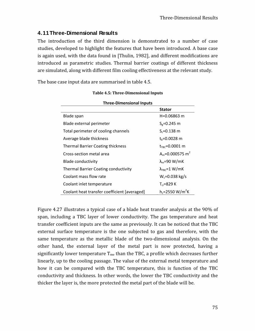
Three-Dimensional Results
75
4.11 Three-Dimensional Results The introduction of the third dimension is demonstrated to a number of case studies, developed to highlight the features that have been introduced. A base case is again used, with the data found in [Thulin, 1982], and different modifications are introduced as parametric studies. Thermal barrier coatings of different thickness are simulated, along with different film cooling effectiveness at the relevant study.
The base case input data are summarised in table 4.5.
Table 4.5: Three-Dimensional Inputs
Three-Dimensional Inputs Stator Blade span H=0.06863 m Blade external perimeter Sg=0.245 m Total perimeter of cooling channels Sc=0.138 m Average blade thickness tb=0.0028 m Thermal Barrier Coating thickness tTBC=0.0001 m Cross-section metal area Am=0.000575 m2 Blade conductivity λm=90 W/mK Thermal Barrier Coating conductivity λTBC=1 W/mK Coolant mass flow rate Wc=0.038 kg/s Coolant inlet temperature Tci=829 K Coolant heat transfer coefficient [averaged] hc=2550 W/m2K
Figure 4.27 illustrates a typical case of a blade heat transfer analysis at the 90% of span, including a TBC layer of lower conductivity. The gas temperature and heat transfer coefficient inputs are the same as previously. It can be noticed that the TBC external surface temperature is the one subjected to gas and therefore, with the same temperature as the metallic blade of the two-dimensional analysis. On the other hand, the external layer of the metal part is now protected, having a significantly lower temperature Tme than the TBC, a profile which decreases further linearly, up to the cooling passage. The value of the external metal temperature and how it can be compared with the TBC temperature, this is function of the TBC conductivity and thickness. In other words, the lower the TBC conductivity and the thicker the layer is, the more protected the metal part of the blade will be.

Three-Dimensional Results
76
4.27: Finite blade thickness effect at 0.9 span
Indeed, Figure 4.28 illustrates two different TBC configurations, with thicknesses of 0.05mm and 0.2mm and the same conductivity. The results in temperature decrease are evident, as a thicker TBC implies a higher Biot number and therefore, a better protected metal part of the blade.
800
900
1000
1100
1200
1300
1400
1500
1600
1700
1800
0 0.25 0.5 0.75 1
Tem
pera
ture
[K]
Fraction of Perimeter
Tg
TTBC
Tc
Blade layers Tm external
Tm internal
Trailing edge
Pressure side
Suction side
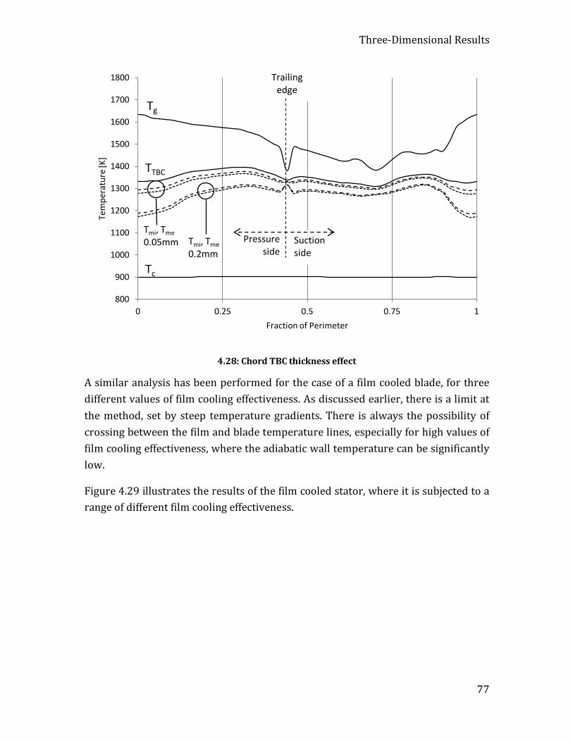
Three-Dimensional Results
77
4.28: Chord TBC thickness effect
A similar analysis has been performed for the case of a film cooled blade, for three different values of film cooling effectiveness. As discussed earlier, there is a limit at the method, set by steep temperature gradients. There is always the possibility of crossing between the film and blade temperature lines, especially for high values of film cooling effectiveness, where the adiabatic wall temperature can be significantly low.
Figure 4.29 illustrates the results of the film cooled stator, where it is subjected to a range of different film cooling effectiveness.
800
900
1000
1100
1200
1300
1400
1500
1600
1700
1800
0 0.25 0.5 0.75 1
Tem
pera
ture
[K]
Fraction of Perimeter
Trailing edge
Pressure side
Suction side
Tg
TTBC
Tc
Tmi, Tme 0.05mm Tmi, Tme
0.2mm
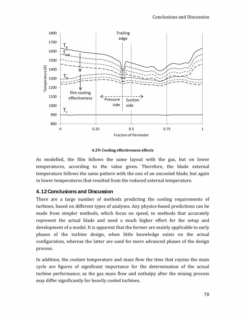
Conclusions and Discussion
78
4.29: Cooling effectiveness effects
As modelled, the film follows the same layout with the gas, but on lower temperatures, according to the value given. Therefore, the blade external temperature follows the same pattern with the one of an uncooled blade, but again in lower temperatures that resulted from the reduced external temperature.
4.12 Conclusions and Discussion There are a large number of methods predicting the cooling requirements of turbines, based on different types of analyses. Any physics-based predictions can be made from simpler methods, which focus on speed, to methods that accurately represent the actual blade and need a much higher effort for the setup and development of a model. It is apparent that the former are mainly applicable to early phases of the turbine design, when little knowledge exists on the actual configuration, whereas the latter are used for more advanced phases of the design process.
In addition, the coolant temperature and mass flow the time that rejoins the main cycle are figures of significant importance for the determination of the actual turbine performance, as the gas mass flow and enthalpy after the mixing process may differ significantly for heavily cooled turbines.
800
900
1000
1100
1200
1300
1400
1500
1600
1700
1800
0 0.25 0.5 0.75 1
Tem
pera
ture
[K]
Fraction of Perimeter
Trailing edge
Pressure side
Suction side
Tg
Tb
Tc
Taw
film cooling effectiveness
Conclusions and Discussion
79
The simpler, analytical or semi-empirical methods discussed earlier do not offer a resolution at the chord direction, which can affect the results, as the flow varies significantly at the axial direction. In addition, the modelling of conduction was proved to affect the blade temperature results as well, which is neglected with the earlier methods.
On the other hand, the more complex, numerical methods that can simulate the problem with a more accurate geometry and higher fidelity are complex to setup and very time-consuming. In addition, the moment when a designer knows the internal geometry in details, this is an advanced phase of the design process.
Therefore, the presented method is mainly applicable at an early stage of the design or the evaluation of an existing design, when not many information exist for the final outcome. The relatively limited number of inputs required means that the evaluation and parametric analysis of many different configurations is favourable. In addition, as the method can feed a gas turbine performance simulation program with data for the turbine coolant, the light computational requirements ensure that the code can be easily coupled with the performance module.
Revising the method fundamentals and findings, the blade is modeled as a heat exchanger between the gas and coolant, with a single internal cooling channel with averaged heat transfer properties. The method includes individual treating of discrete blade elements in span and chord directions and accounts the effects of thermal diffusion due to conduction in both directions. The inclusion of conduction modeling is important, as diffusion tends to moderate steep blade temperature slopes, affecting both the performance and life of it.
In addition, the variable resolution adds to the method fidelity, as it can be independently selected by the user. The importance of high resolution gas inputs is highlighted as well, as the vast gas acceleration and expansion in turbines has a significant effect on the gas static and total temperature, a process usually ignored when no flow simulation is performed, with the use of station averaged gas properties instead. Both stator and rotor studies can be performed, as the difference lies on suitable data input as boundary conditions.
Moreover, the method is completed with the addition of conductivity modeling in the third (thickness) direction. Here, the approach is based on Biot number analysis. This kind of modeling adds the feature of a finite blade thickness, with a predicted temperature gradient as an output, along with provision for multiple blade layers,

Conclusions and Discussion
80
such as Thermal Barrier Coatings. Therefore, the metal temperature can be calculated at any blade point and the influence of the TBC can be assessed. The method has been developed for the preliminary phase of the design of turbines, where no experiments or sophisticated CFD investigations are essential. Empirical inputs can be equally used or simple flow solvers, such as Euler-based methods for the definition of the necessary boundary conditions.
A main method limitation is that a detailed picture of the gas flow field is required, i.e. gas temperature and heat transfer coefficient. That information is usually more difficult to obtain compared to averaged values at different engine stations. Uniform gas inputs are an option as well in any of the two directions, reducing the resolution by one dimension in the case of uniform chord gas state. If the span gas temperature and coefficient profile remain constant along the span, this results again to a variable blade and coolant temperature at the span direction, as the coolant heats up and provides reduced cooling capability towards this direction.
As, the internal cooling system is not modeled in detail, the model simulates a single cooling channel with an averaged heat transfer coefficient. The result of this is a metal temperature that is just indicative of the reality and not predicted in detail. On the other hand, that was a conscious design decision, as a detailed representation of the actual geometry would be extremely challenging and long.
81
5 Multistage Cooled Turbine Simulation
5.1 Gas Turbine Performance Simulation
5.1.1 Introduction A significant number of gas turbine simulation codes were developed throughout the years, with different intended use and fidelity. Accuracy in results is always a requirement, but this means that most times a higher accuracy or a higher order of fidelity usually increases the complexity of the method, the execution time, and inevitably, the number of inputs. In other words, it appears that fidelity most times increases complexity as well.
Therefore, all the gas turbine performance simulation codes can be classified into different categories, according to their specifications, mostly derived as a result of the use and a trade-off analysis between the two driving factors. Some codes focus on speed and flexibility, whereas others aim for the accurate prediction of the physics. The first group is used for cycle analysis mainly, where different conceptual engine designs can be simulated and assessed, while the second group usually focuses more on conceptual component design and the basic parameters associated with this procedure.
Another field of differentiation is the code structure, where again different code philosophies emphasise on different modes of use. A more fixed structure is in favour of stability, while inevitably limiting the flexibility of the tool. In contrast, a
Gas Turbine Performance Simulation
82
more modular structure facilitates the simulation of different concepts and designs, but affects stability and user friendliness.
Simulation of the engine turbine, as an essential part of any performance code is treated with different degrees of fidelity and structure by different developers: From zero-dimensional to fully three-dimensional and from externally coupled, to fully integrated to the code. Again, every application requires a different approach and this is the reason that a number of different turbine simulation methods have been developed.
5.1.2 Degrees of Fidelity As gas turbine simulation follows the evolution of informatics, it is apparent that the low computational capabilities of the early computers allowed only for low-fidelity simulation codes. Low-fidelity codes are still in great use until today, as their main application is to provide an overview of the engine performance under a certain thermodynamic cycle. In parallel, a number of higher fidelity codes has been developed throughout the years. Following the computers advancements, the simulation of the internal operation of components has been integrated, providing data for the gas state at different axial or even radial positions [Denton, 1998].
Gas turbine simulation programs can be classified according to the maximum dimensions of resolution being able to provide, varying from zero- to three-dimensional. A zero-dimensional code means that the engine components act as black boxes [MacMillan, 1974], where no output information is provided for their internal performance. No axial, radial or circumferential resolution is provided, and the gas state takes single values at every station calculated. At off-design analysis, the component operation is based on predefined maps that provide the component-averaged performance characteristics for any given operating condition [Kurzke, 1996] [Sieros, 1997] [Kong, 2006].
The benefits associated with such kind of simulations are mainly related to the minimisation of the required time and effort, when a cycle overview is intended, rather that detailed component analysis. The drawbacks are mainly related to the inability of capturing any complex physics on a local level. Typical examples of such kind of codes include GasTurb [Kurzke, 2007], GSP [Visser, 2000] and Turbomatch [Janikovič, 2007].
A higher fidelity code mainly is able to fully or partially provide a higher than zero resolution to some of the engine parts. Flow and performance physics in different
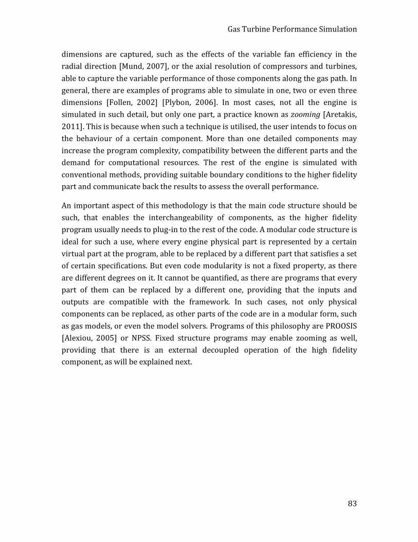
Gas Turbine Performance Simulation
83
dimensions are captured, such as the effects of the variable fan efficiency in the radial direction [Mund, 2007], or the axial resolution of compressors and turbines, able to capture the variable performance of those components along the gas path. In general, there are examples of programs able to simulate in one, two or even three dimensions [Follen, 2002] [Plybon, 2006]. In most cases, not all the engine is simulated in such detail, but only one part, a practice known as zooming [Aretakis, 2011]. This is because when such a technique is utilised, the user intends to focus on the behaviour of a certain component. More than one detailed components may increase the program complexity, compatibility between the different parts and the demand for computational resources. The rest of the engine is simulated with conventional methods, providing suitable boundary conditions to the higher fidelity part and communicate back the results to assess the overall performance.
An important aspect of this methodology is that the main code structure should be such, that enables the interchangeability of components, as the higher fidelity program usually needs to plug-in to the rest of the code. A modular code structure is ideal for such a use, where every engine physical part is represented by a certain virtual part at the program, able to be replaced by a different part that satisfies a set of certain specifications. But even code modularity is not a fixed property, as there are different degrees on it. It cannot be quantified, as there are programs that every part of them can be replaced by a different one, providing that the inputs and outputs are compatible with the framework. In such cases, not only physical components can be replaced, as other parts of the code are in a modular form, such as gas models, or even the model solvers. Programs of this philosophy are PROOSIS [Alexiou, 2005] or NPSS. Fixed structure programs may enable zooming as well, providing that there is an external decoupled operation of the high fidelity component, as will be explained next.
Gas Turbine Performance Simulation
84
5.1: NPSS zooming interconnection platform [Follen, 2000]
According to Follen [2000], the benefits from high fidelity components simulation are three:
• In component design level, every design can be evaluated as part of the engine rather that individually. This improves the engine performance results as well, since a part of the simulation is based on a more sophisticated model.
• The optimisation of the higher fidelity component can be carried out more effectively, as the assessment of every set of results is based in both a local and an engine performance level.
• The resources needed are lower as well in comparison with a fully experimental approach. Any change in design can be directly evaluated for a physics-based component performance model and the more successful designs can be experimentally tested thereafter. By following such a procedure, the amount of experiments needed is lower in comparison with a conventional approach, as commitment to hardware is extremely costly.
5.1.3 High Fidelity Components and Integration with the Main Code There are different ways that virtual engine components communicate with the main code. A component model can be in many cases an integral part of the main program, or it can be a completely externally managed self-contained program. Between the two extremes, there are different levels of integration:

Gas Turbine Performance Simulation
85
Decoupled Components
A decoupled simulation approach, as implemented by Melloni [2006], is a procedure where an engine component is a self-contained program that runs externally and independently from the main code. The external component runs on a wide range of different operating conditions that are registered subsequently and produce a performance map. The map is then utilised by a lower fidelity component, integrated to the main code and the performance of the engine is predicted, based on the map, which represents a higher fidelity approach. An example of such a scheme is given by Alexiou [2007], where an one-dimensional compressor, assembled with the use of a stage-stacking method is simulated by PROOSIS with both three coupling methods.
Semi-Coupled Components
A semi-coupled approach follows the same layout with the decoupled mode, where an engine component runs externally from the main engine performance program. The difference with previously is that the external program runs on demand of the main code and not indepedently, producing maps. Indeed, when a certain simulation starts, the main program provides the external module with a set of boundary conditions and specifications. The component then performs a simulation based on those inputs and communicates back to the main code a set of results. In the case of an off design simulation, this process is repeated with different inputs every time, until an equilibrium among the performance of all components is achieved. Back to the main program, the results communicated back from the external module may be directly addressed to the other engine parts, or indirectly through the use of maps. In this case, a lower-fidelity component that utilises maps represents the external one and scales them according to the results communicated back. A typical example of this approach is given by Pachidis [2006a], where a three-dimensional CFD intake model is externally simulated, in coupling with a performance code named PYTHIA, developed by the Department of Power & Propulsion of Cranfield University. Another example of such an approach follows at the paragraph 5.8 of this chapter.
Integrated Components
The third and final coupling mode for the communication of external engine components is a component is integrated with the main code. At this approach, the main program is developed in a way that can fully operate the higher fidelity component without the intervention of an equivalent lower-fidelity, acting as the
The Cooled Turbine – A Literature Survey
86
messenger between them. The higher fidelity model is able to directly receive data and handled by the main program, it calculates the component performance results based on a certain model and communicates the results back to the main code, in order to calculate the overall performance. An example of a fully-coupled engine is given by Hall [2000], where various components based on three-dimensional CFD simulations are integrated into NASA’s NPSS gas turbine performance code.
5.2 The Cooled Turbine – A Literature Survey
5.2.1 Introduction Engine turbines operate in extremely high temperatures that can only be reached with the use of a high amount of efficient cooling. A large amount of resources is required by the engine manufacturers in order to investigate, understand and improve the cooling technology, as a large number of benefits are associated with a more effective cooling. As a result, it can be observed that maximum engine temperatures are constantly increasing, since a higher cycle temperature is associated with benefits in thermal efficiency, until a certain point is reached where chemical reactions become dominant [Sethi, 2008]. On the other hand, higher cycle temperatures usually mean a higher amount of cooling air extraction from the main cycle, a practice with increasing thermal penalties, as Horlock [2001a] observed. Therefore, a more effective cooling for a constant amount of coolant is an important field of research, along with materials and coatings with improved thermal behaviour.
The performance of cooled turbines has been a field of study for many years and a lot of effort has been put towards the understanding of the complex flow and heat transfer effects that take place. As technology improves, there is always ground for new configurations and methods that need to be investigated. More environmentally friendly approaches are currently under research by many programs, and improvements in turbine technology are among the highest priority items.
On a cycle basis, the need for more sophisticated turbine performance prediction tools is important, as cooling is a dominant aspect of the overall turbine behaviour. A more accurate or comprehensive turbine performance prediction enables the assessment of cooling effects otherwise ignored or underestimated.
The Cooled Turbine – A Literature Survey
87
5.2.2 Turbine Aero-Thermodynamics and Efficiency
5.2.2.1 Working Fluid Composition Modelling According to Young [2002a] the working fluid composition modelling is an important aspect of turbine simulation. They suggested that the degree of accuracy needed cannot be reached with a perfect gas model and varying Cp and gamma properties. Since the composition of the exhaust gases varies according to the combustion process, the fuel composition and the fuel-to-air ratio, they suggest that a satisfactory model should acknowledge the various gases that compose the main gas. A semi-perfect mixture of N2, O2, CO2 and H2O is therefore suggested, with temperature dependent Cp and gamma properties.
Another modelling approach by Young suggests that a fluid model composed by air and gas and properties defined according to their component synthesis is acceptable as well under certain conditions. Following, they examine the entropy creation in compositional mixing. They state that entropy is created in every irreversible diffusion mixing of air and gas, and this is unavoidable under the conditions that mixing takes place. Following, they examine the influence of the station that mixing takes place: Ahead or behind the rotor. They observe that with ideal gas components the power output is not affected. However, with pressure dependant Cp and gamma, the mixing created entropy is dependent as well and the power output and efficiency of the turbine are affected.
5.2.2.2 Turbine Efficiency The determination of turbine efficiency is a topic of extensive discussion. Until today, there is no standard way for the definition of it, making the communication of associated figures a task that needs caution. The difficulty in defining a commonly used accounting method is that turbine cooling complicates the calculations, since the definition of an ideal turbine operation is ambiguous.
Young and Horlock [2006] have tried to register the various definitions and methods. A first classification can be made between cooled and un-cooled turbines. A universal definition applicable in all cases is the following:
S
TWnTW
= (5.1)
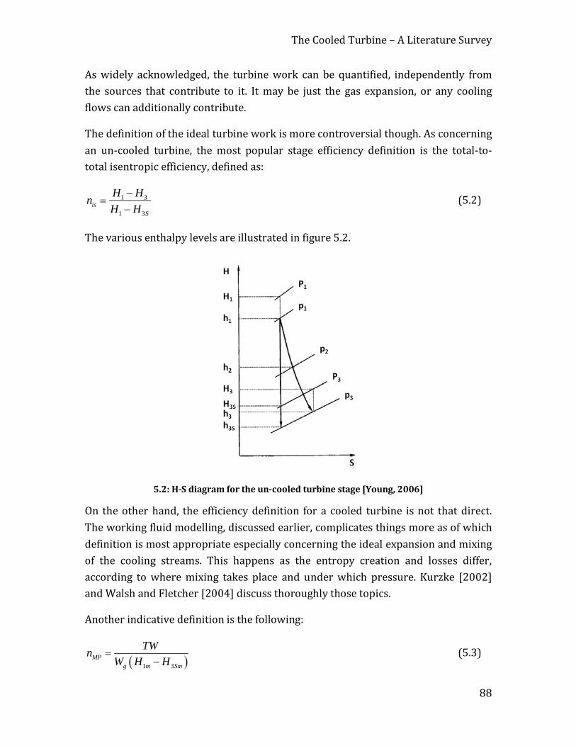
The Cooled Turbine – A Literature Survey
88
As widely acknowledged, the turbine work can be quantified, independently from the sources that contribute to it. It may be just the gas expansion, or any cooling flows can additionally contribute.
The definition of the ideal turbine work is more controversial though. As concerning an un-cooled turbine, the most popular stage efficiency definition is the total-to-total isentropic efficiency, defined as:
1 3
1 3is
S
H HnH H
−=
− (5.2)
The various enthalpy levels are illustrated in figure 5.2.
5.2: H-S diagram for the un-cooled turbine stage [Young, 2006]
On the other hand, the efficiency definition for a cooled turbine is not that direct. The working fluid modelling, discussed earlier, complicates things more as of which definition is most appropriate especially concerning the ideal expansion and mixing of the cooling streams. This happens as the entropy creation and losses differ, according to where mixing takes place and under which pressure. Kurzke [2002] and Walsh and Fletcher [2004] discuss thoroughly those topics.
Another indicative definition is the following:
( )1 3MP
g m Sm
TWnW H H
=−
(5.3)
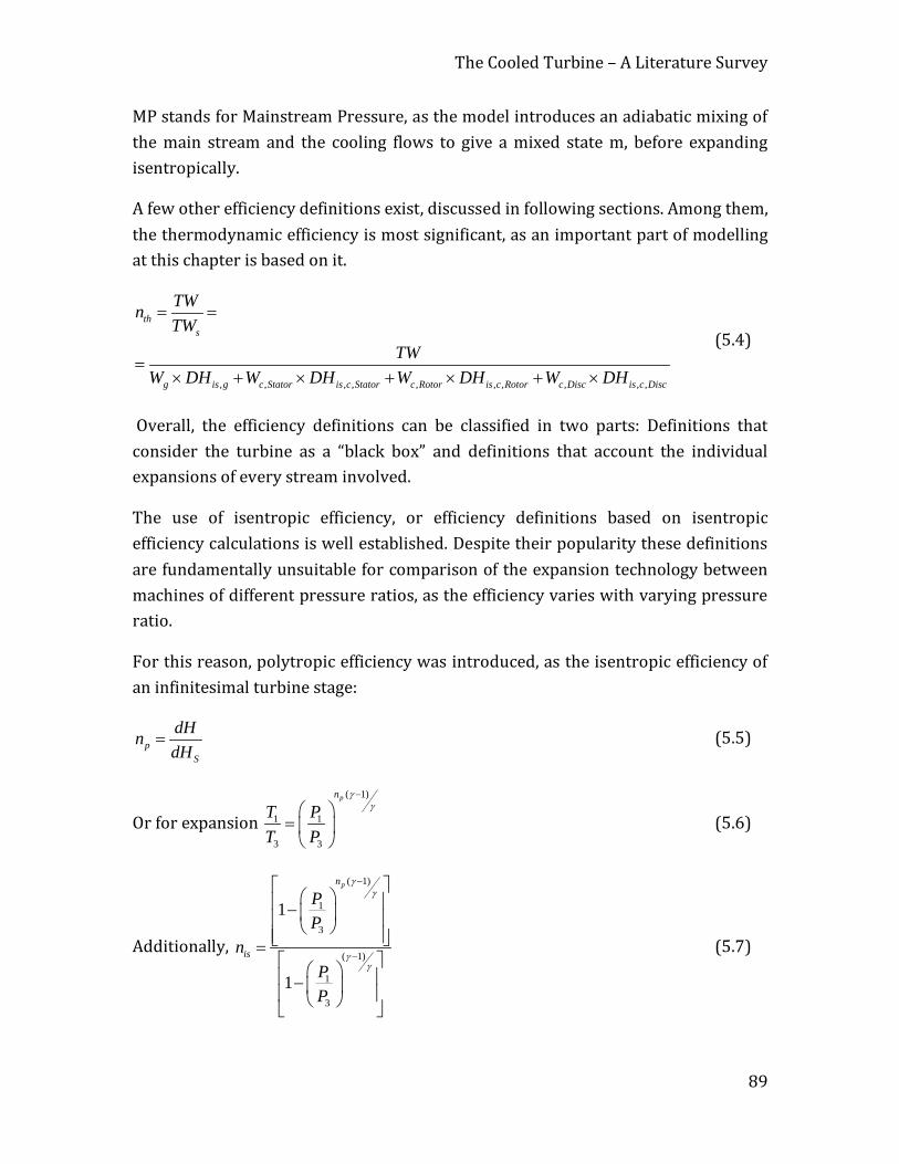
The Cooled Turbine – A Literature Survey
89
MP stands for Mainstream Pressure, as the model introduces an adiabatic mixing of the main stream and the cooling flows to give a mixed state m, before expanding isentropically.
A few other efficiency definitions exist, discussed in following sections. Among them, the thermodynamic efficiency is most significant, as an important part of modelling at this chapter is based on it.
, , , , , , , , , ,
ths
g is g c Stator is c Stator c Rotor is c Rotor c Disc is c Disc
TWnTW
TWW DH W DH W DH W DH
= =
=× + × + × + ×
(5.4)
Overall, the efficiency definitions can be classified in two parts: Definitions that consider the turbine as a “black box” and definitions that account the individual expansions of every stream involved.
The use of isentropic efficiency, or efficiency definitions based on isentropic efficiency calculations is well established. Despite their popularity these definitions are fundamentally unsuitable for comparison of the expansion technology between machines of different pressure ratios, as the efficiency varies with varying pressure ratio.
For this reason, polytropic efficiency was introduced, as the isentropic efficiency of an infinitesimal turbine stage:
pS
dHndH
= (5.5)
Or for expansion
( 1)
1 1
3 3
pn
T PT P
γγ
−
=
(5.6)
Additionally,
( 1)
1
3
( 1)
1
3
1
1
pn
is
PP
nPP
γγ
γγ
−
−
− =
−
(5.7)
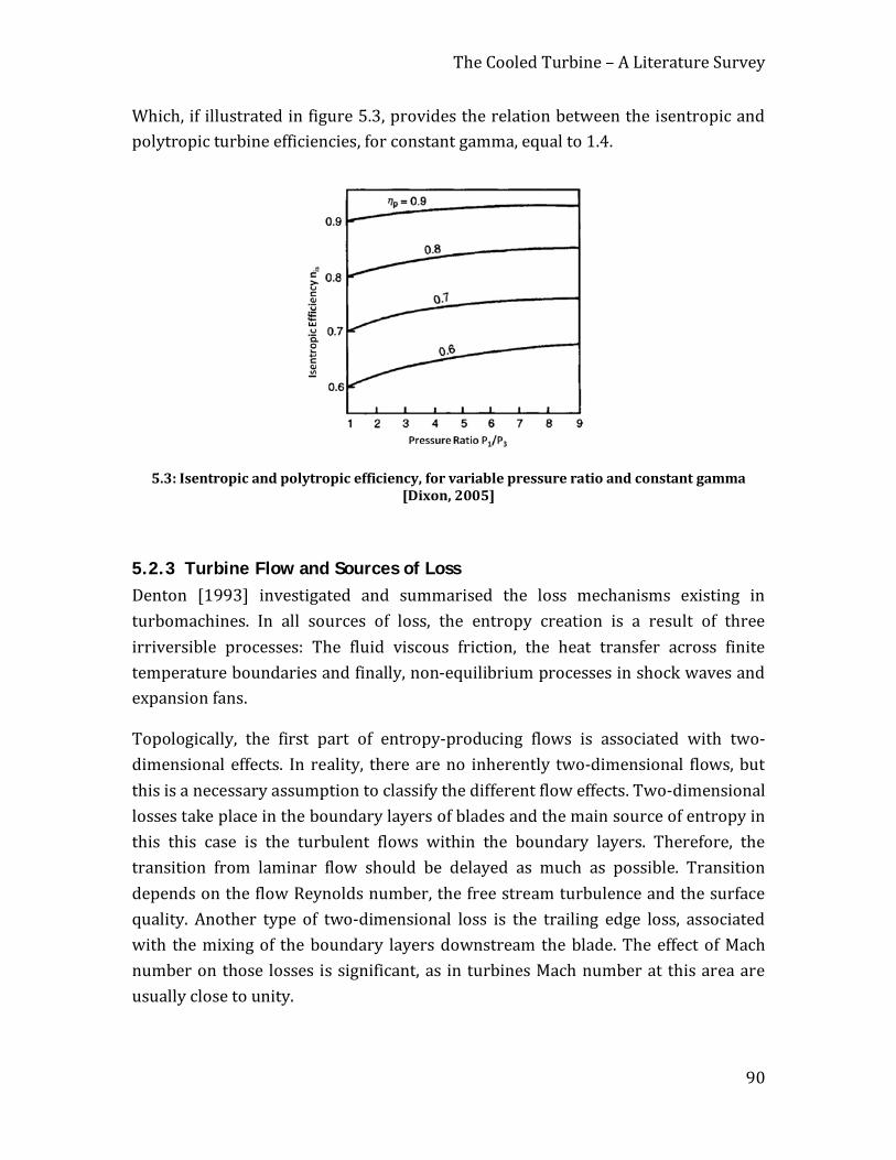
The Cooled Turbine – A Literature Survey
90
Which, if illustrated in figure 5.3, provides the relation between the isentropic and polytropic turbine efficiencies, for constant gamma, equal to 1.4.
5.3: Isentropic and polytropic efficiency, for variable pressure ratio and constant gamma [Dixon, 2005]
5.2.3 Turbine Flow and Sources of Loss Denton [1993] investigated and summarised the loss mechanisms existing in turbomachines. In all sources of loss, the entropy creation is a result of three irriversible processes: The fluid viscous friction, the heat transfer across finite temperature boundaries and finally, non-equilibrium processes in shock waves and expansion fans.
Topologically, the first part of entropy-producing flows is associated with two-dimensional effects. In reality, there are no inherently two-dimensional flows, but this is a necessary assumption to classify the different flow effects. Two-dimensional losses take place in the boundary layers of blades and the main source of entropy in this this case is the turbulent flows within the boundary layers. Therefore, the transition from laminar flow should be delayed as much as possible. Transition depends on the flow Reynolds number, the free stream turbulence and the surface quality. Another type of two-dimensional loss is the trailing edge loss, associated with the mixing of the boundary layers downstream the blade. The effect of Mach number on those losses is significant, as in turbines Mach number at this area are usually close to unity.
The Cooled Turbine – A Literature Survey
91
The second part of entropy-producing effects is the flows at the area of blade tips, where tip leakages take place. Bindon [1989] investigated thoroughly the the mechanisms that lead to tip leakage losses. The most dominant effect is the turbine mass flow increase, with a simultaneous reduced pressure drop, in both shrouded and unshrouded blades. In shrouded blades, the entropy creation is mainly attributed to the mixing of the leakage flow with the mainstream flow. In unshrouded blades, the secondary flow enters the tip gap at the pressure side, due to pressure differential and subsequently separates from the blade, forming a local jet. Following, the jet is mixed with the main stream, forming a vortex that may propagate downstream.
Endwall loss is the third source of loss in turbomachinery flows. It remains relatively unexplored, even today and the loss mechanisms are still unclear, although it highly contributes to the lost efficiency in turbines. The prediction of enwall losses is still widely based on empirical correlations. Dunham and Came [1970] developed an empirical correlation that predicts the overall efficiency, although they discovered that loss in actual machines is a few times the loss measured in their experimental cascades. An endwall boundary layer is formed upstream the blade, and as approaching, it separates and forms a horseshoe vortex. The streams then incline to the blade suction side, approach the boundary layer at the trailing edge and form a region of high entropy creation.
Overall, these flow properties are mainly contributing to the entropy creation in turbines and along with cooling, the main topics in aero- and thermodynamics investigation topics on turbine turbomachinery. The contribution of these effects to the turbine efficiency is dominant. In many cases, they can empirically modelled and accounted in a joined way.
5.2.4 Turbine Modelling
5.2.4.1 Standard Turbine Modelling The current standard industrial approach in turbine modelling is zero-dimensional. This means that the turbine is not represented with any physical dimensions. In contrast, it is accounted as a “black box”, where the gas condition changes from the inlet to the outlet based on certain mathematical correlations. The off-design point performance of the turbine is based on component maps that guide the expansion process between the inlet and outlet stations. The presence of any physically turbine stages is neglected and the gas is considered to expand between the two pressure
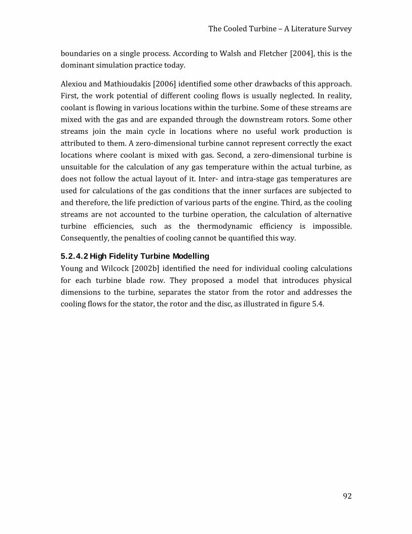
The Cooled Turbine – A Literature Survey
92
boundaries on a single process. According to Walsh and Fletcher [2004], this is the dominant simulation practice today.
Alexiou and Mathioudakis [2006] identified some other drawbacks of this approach. First, the work potential of different cooling flows is usually neglected. In reality, coolant is flowing in various locations within the turbine. Some of these streams are mixed with the gas and are expanded through the downstream rotors. Some other streams join the main cycle in locations where no useful work production is attributed to them. A zero-dimensional turbine cannot represent correctly the exact locations where coolant is mixed with gas. Second, a zero-dimensional turbine is unsuitable for the calculation of any gas temperature within the actual turbine, as does not follow the actual layout of it. Inter- and intra-stage gas temperatures are used for calculations of the gas conditions that the inner surfaces are subjected to and therefore, the life prediction of various parts of the engine. Third, as the cooling streams are not accounted to the turbine operation, the calculation of alternative turbine efficiencies, such as the thermodynamic efficiency is impossible. Consequently, the penalties of cooling cannot be quantified this way.
5.2.4.2 High Fidelity Turbine Modelling Young and Wilcock [2002b] identified the need for individual cooling calculations for each turbine blade row. They proposed a model that introduces physical dimensions to the turbine, separates the stator from the rotor and addresses the cooling flows for the stator, the rotor and the disc, as illustrated in figure 5.4.
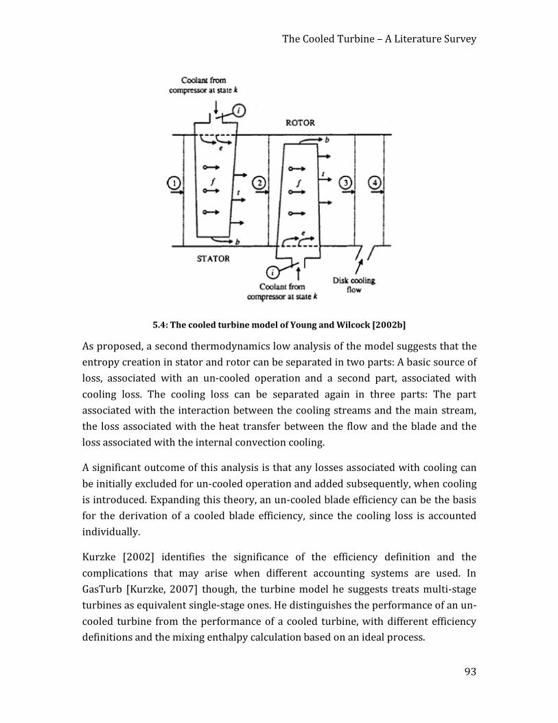
The Cooled Turbine – A Literature Survey
93
5.4: The cooled turbine model of Young and Wilcock [2002b]
As proposed, a second thermodynamics low analysis of the model suggests that the entropy creation in stator and rotor can be separated in two parts: A basic source of loss, associated with an un-cooled operation and a second part, associated with cooling loss. The cooling loss can be separated again in three parts: The part associated with the interaction between the cooling streams and the main stream, the loss associated with the heat transfer between the flow and the blade and the loss associated with the internal convection cooling.
A significant outcome of this analysis is that any losses associated with cooling can be initially excluded for un-cooled operation and added subsequently, when cooling is introduced. Expanding this theory, an un-cooled blade efficiency can be the basis for the derivation of a cooled blade efficiency, since the cooling loss is accounted individually.
Kurzke [2002] identifies the significance of the efficiency definition and the complications that may arise when different accounting systems are used. In GasTurb [Kurzke, 2007] though, the turbine model he suggests treats multi-stage turbines as equivalent single-stage ones. He distinguishes the performance of an un-cooled turbine from the performance of a cooled turbine, with different efficiency definitions and the mixing enthalpy calculation based on an ideal process.
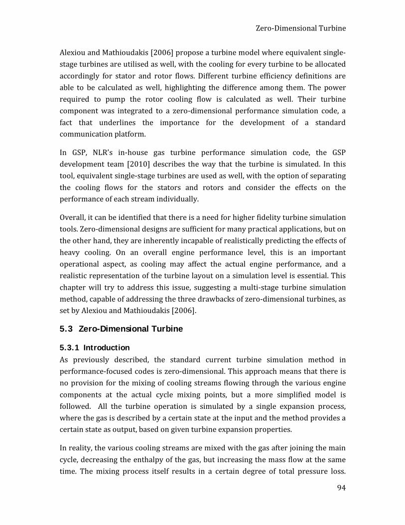
Zero-Dimensional Turbine
94
Alexiou and Mathioudakis [2006] propose a turbine model where equivalent single-stage turbines are utilised as well, with the cooling for every turbine to be allocated accordingly for stator and rotor flows. Different turbine efficiency definitions are able to be calculated as well, highlighting the difference among them. The power required to pump the rotor cooling flow is calculated as well. Their turbine component was integrated to a zero-dimensional performance simulation code, a fact that underlines the importance for the development of a standard communication platform.
In GSP, NLR’s in-house gas turbine performance simulation code, the GSP development team [2010] describes the way that the turbine is simulated. In this tool, equivalent single-stage turbines are used as well, with the option of separating the cooling flows for the stators and rotors and consider the effects on the performance of each stream individually.
Overall, it can be identified that there is a need for higher fidelity turbine simulation tools. Zero-dimensional designs are sufficient for many practical applications, but on the other hand, they are inherently incapable of realistically predicting the effects of heavy cooling. On an overall engine performance level, this is an important operational aspect, as cooling may affect the actual engine performance, and a realistic representation of the turbine layout on a simulation level is essential. This chapter will try to address this issue, suggesting a multi-stage turbine simulation method, capable of addressing the three drawbacks of zero-dimensional turbines, as set by Alexiou and Mathioudakis [2006].
5.3 Zero-Dimensional Turbine
5.3.1 Introduction As previously described, the standard current turbine simulation method in performance-focused codes is zero-dimensional. This approach means that there is no provision for the mixing of cooling streams flowing through the various engine components at the actual cycle mixing points, but a more simplified model is followed. All the turbine operation is simulated by a single expansion process, where the gas is described by a certain state at the input and the method provides a certain state as output, based on given turbine expansion properties.
In reality, the various cooling streams are mixed with the gas after joining the main cycle, decreasing the enthalpy of the gas, but increasing the mass flow at the same time. The mixing process itself results in a certain degree of total pressure loss.

Zero-Dimensional Turbine
95
Moreover, the time a proportion of the cooling air joins the main cycle, affects the performance of the components downstream. To give an example, again in the case of a two-stage HPT, the cooling stream of the NGV is a part of the gas for the first stage rotor and the whole second stage.
The main assumption here is that there are streams accounted to the expansion process through a rotor and streams that do not. Again, single- and two-stage turbines differentiate on the accuracy of the results, as in the case of the latter more assumptions are necessary.
By using a zero-dimensional model, there are a number of options for the simulation of a cooled multi-stage HPT. It is common ground to assume that there are three cooling streams for each stage [Kurzke, 2002], each one of them individually treated by the method. The first stream represents the cooling of the stator vanes, the second stream represents the rotor blade cooling and the third stream represents the disc and casing cooling streams.
In table 5.1, the cooling streams accounted for each turbine model are illustrated:
Table 5.1: Cooling streams accounted for different turbine models
2-stage 1-stage 0-D NGV stream NGV stream -
1st rotor stream Rotor stream 1st disc stream Disc stream
2nd stator stream 2nd rotor stream 2nd disc stream
As the input to a zero-dimensional turbine, that performs just the expansion, is controlled by the user, the mixing of a proportion of the total HPT cooling air upstream the component is possible. This proportion represents coolant that contributes to the work produced by both rotors. This can be the coolant provided to the NGV. Equivalently, a proportion of the cooling air can be mixed with the main stream downstream the turbine component. This typically represents the second rotor and disc cooling, as it is assumed that they do not contribute at any work produced by the HPT. There is though, a significant part of the coolant that is should not be mixed in any of the two mixing points. These are typically the cooling streams for the first stage rotor and disc and the second stage stator that contribute only to a
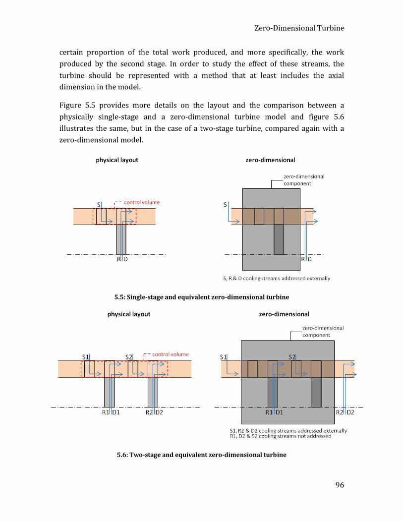
Zero-Dimensional Turbine
96
certain proportion of the total work produced, and more specifically, the work produced by the second stage. In order to study the effect of these streams, the turbine should be represented with a method that at least includes the axial dimension in the model.
Figure 5.5 provides more details on the layout and the comparison between a physically single-stage and a zero-dimensional turbine model and figure 5.6 illustrates the same, but in the case of a two-stage turbine, compared again with a zero-dimensional model.
5.5: Single-stage and equivalent zero-dimensional turbine
5.6: Two-stage and equivalent zero-dimensional turbine
Zero-Dimensional Turbine
97
In the case of a single-stage HPT, it is apparent that the stream allocation is not a restriction anymore. The assumed three discrete cooling streams can be simulated individually, with the NGV cooling mixed upstream and the rotor, disc and casing cooling mixed downstream the virtual turbine. But again, as the zero-dimensional turbine is performing just the expansion process, the mixing processes are handled externally. As a result, the efficiency reported by the component is the turbine isentropic efficiency, which is indicative of the technology level, but not indicative of the actual process that takes place with the certain cooling specifications. This last issue can only be addressed with a turbine component that includes the handling of the mixing processes of the three cooling streams.
Therefore, the results of a zero-dimensional turbine model neglect three different areas:
First, the work produced may deviate by neglecting the contribution of the cooling streams expanded through the second stage rotor. This is an additional source of error in respect to the predicted turbine work that affects the operating point and the overall performance simulation. This may be projected to the cost and feasibility assessment of a certain layout during the preliminary design phase, affecting the decision process concerning the chosen cycle parameters.
Second, it is impossible to calculate the different inter-stage temperatures for the same reason. The prediction of a certain inter-stage temperature at the HPT is an important input for the preliminary thermal design of the turbomachinery components and a crucial life determining factor.
Third, the actual cooled turbine efficiency is different from the turbine isentropic efficiency, and impossible to be calculated without accounting the contribution of each individual cooling stream. As previously discussed, the cooled turbine efficiency is a figure that describes more accurately the process that takes place and it is more indicative of the actual turbine performance. As a result, it helps the communication of results among different teams, as it gives a better indication of how the physical component performs.
5.3.2 Method A zero-dimensional turbine module working independently from the main gas turbine program (semi-coupled mode) controls just one expansion process. Hence, the layout of the component structure is fairly simple. The necessary inputs for the gas condition include the total pressure and temperature, fuel-to-air ratio and mass
Zero-Dimensional Turbine
98
flow at the inlet. In addition, the turbine pressure ratio or enthalpy drop is necessary, along with the isentropic efficiency to calculate the expansion output quantities.
As the heat capacity of the gas Cp is a function of the gas fuel-to-air ratio and the gas temperature, it can be calculated at the turbine input, using a suitable model, such as the one described by Walsh [2004]:
( ), ,p i i iC f FAR T= (5.8)
With the heat capacity known, the total enthalpy per mass unit at the inlet is calculated as:
,i p i iH C T= × (5.9)
Passing to the turbine output, the total fuel-to-air ratio and mass flow rate remain the same, as there is no any source or sink of mass inside the zero-dimensional module.
i o
gi go
FAR FARW W
==
(5.10) & (5.11)
The total pressure of the gas at the outlet can be calculated by the specified pressure ratio:
/o iP P PR= (5.12)
Or alternatively, the total enthalpy at the outlet can be calculated by using the specified enthalpy drop ratio:
/o iH H DH= (5.13)
By having the total outlet pressure or the total outlet enthalpy, the ideal total outlet temperature can be calculated as following, in the case of the former:
1,s o o
i i
T PT P
γγ −
=
(5.14)
With /p vC Cγ = (5.15)
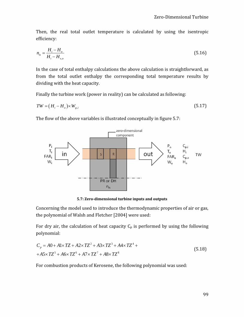
Zero-Dimensional Turbine
99
Then, the real total outlet temperature is calculated by using the isentropic efficiency:
,
i ois
i s o
H HnH H
−=
− (5.16)
In the case of total enthalpy calculations the above calculation is straightforward, as from the total outlet enthalpy the corresponding total temperature results by dividing with the heat capacity.
Finally the turbine work (power in reality) can be calculated as following:
( ) ,i o g iTW H H W= − × (5.17)
The flow of the above variables is illustrated conceptually in figure 5.7:
5.7: Zero-dimensional turbine inputs and outputs
Concerning the model used to introduce the thermodynamic properties of air or gas, the polynomial of Walsh and Fletcher [2004] were used:
For dry air, the calculation of heat capacity Cp is performed by using the following polynomial:
2 3 4
5 6 7 8
0 1 2 3 4
5 6 7 8pC A A TZ A TZ A TZ A TZ
A TZ A TZ A TZ A TZ
= + × + × + × + × +
+ × + × + × + × (5.18)
For combustion products of Kerosene, the following polynomial was used:
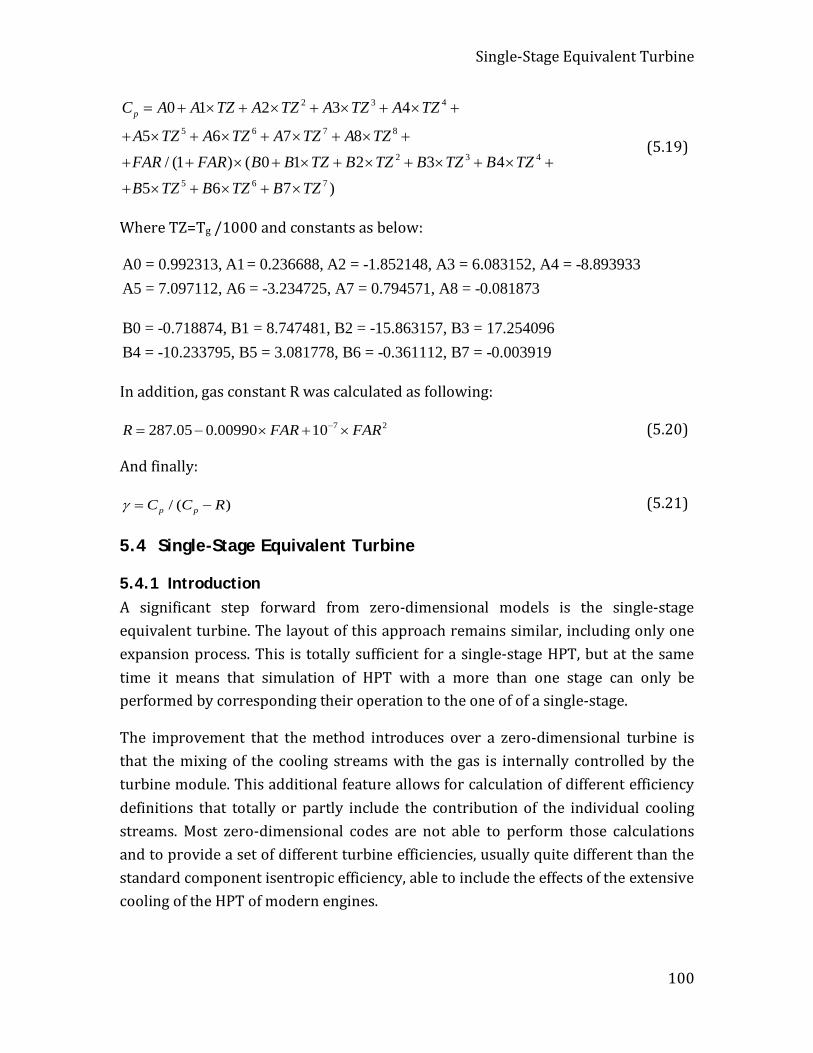
Single-Stage Equivalent Turbine
100
2 3 4
5 6 7 8
2 3 4
5 6 7
0 1 2 3 4
5 6 7 8/ (1 ) ( 0 1 2 3 4
5 6 7 )
pC A A TZ A TZ A TZ A TZ
A TZ A TZ A TZ A TZFAR FAR B B TZ B TZ B TZ B TZB TZ B TZ B TZ
= + × + × + × + × +
+ × + × + × + × +
+ + × + × + × + × + × +
+ × + × + ×
(5.19)
Where TZ=Tg /1000 and constants as below:
A0 = 0.992313, A1 = 0.236688, A2 = -1.852148, A3 = 6.083152, A4 = -8.893933A5 = 7.097112, A6 = -3.234725, A7 = 0.794571, A8 = -0.081873
B0 = -0.718874, B1 = 8.747481, B2 = -15.863157, B3 = 17.254096B4 = -10.233795, B5 = 3.081778, B6 = -0.361112, B7 = -0.003919
In addition, gas constant R was calculated as following:
7 2287.05 0.00990 10R FAR FAR−= − × + × (5.20)
And finally:
/ ( )p pC C Rγ = − (5.21)
5.4 Single-Stage Equivalent Turbine
5.4.1 Introduction A significant step forward from zero-dimensional models is the single-stage equivalent turbine. The layout of this approach remains similar, including only one expansion process. This is totally sufficient for a single-stage HPT, but at the same time it means that simulation of HPT with a more than one stage can only be performed by corresponding their operation to the one of of a single-stage.
The improvement that the method introduces over a zero-dimensional turbine is that the mixing of the cooling streams with the gas is internally controlled by the turbine module. This additional feature allows for calculation of different efficiency definitions that totally or partly include the contribution of the individual cooling streams. Most zero-dimensional codes are not able to perform those calculations and to provide a set of different turbine efficiencies, usually quite different than the standard component isentropic efficiency, able to include the effects of the extensive cooling of the HPT of modern engines.
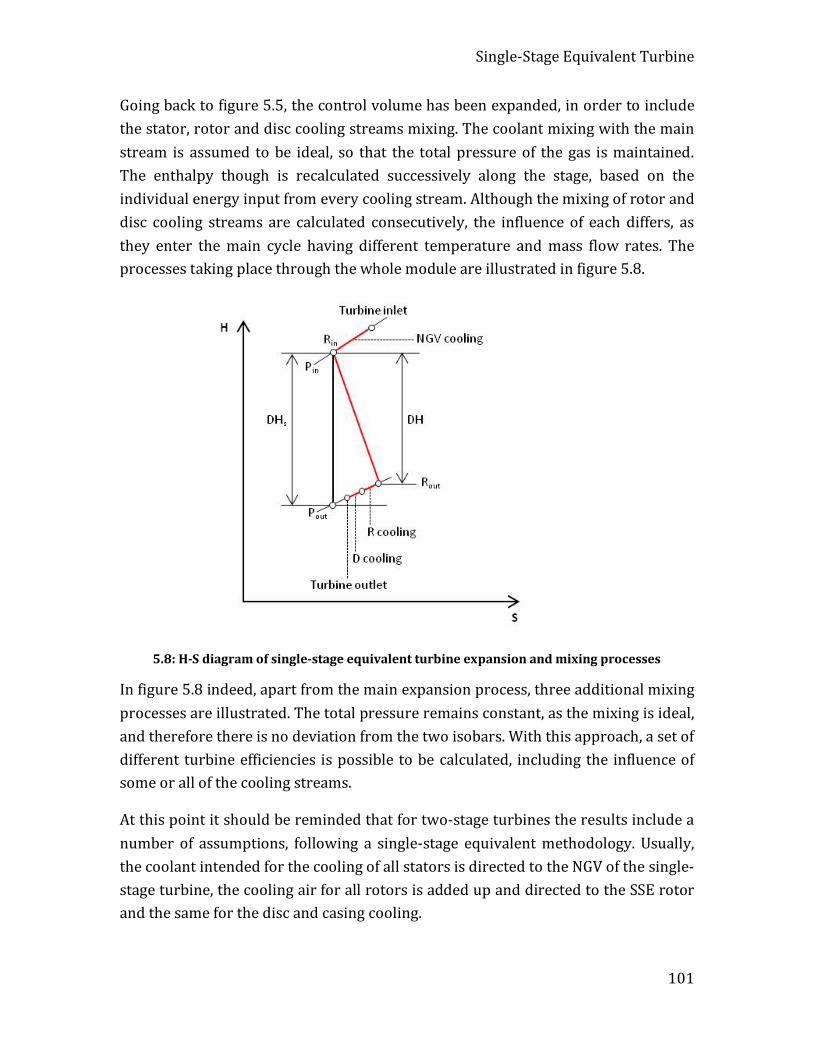
Single-Stage Equivalent Turbine
101
Going back to figure 5.5, the control volume has been expanded, in order to include the stator, rotor and disc cooling streams mixing. The coolant mixing with the main stream is assumed to be ideal, so that the total pressure of the gas is maintained. The enthalpy though is recalculated successively along the stage, based on the individual energy input from every cooling stream. Although the mixing of rotor and disc cooling streams are calculated consecutively, the influence of each differs, as they enter the main cycle having different temperature and mass flow rates. The processes taking place through the whole module are illustrated in figure 5.8.
5.8: H-S diagram of single-stage equivalent turbine expansion and mixing processes
In figure 5.8 indeed, apart from the main expansion process, three additional mixing processes are illustrated. The total pressure remains constant, as the mixing is ideal, and therefore there is no deviation from the two isobars. With this approach, a set of different turbine efficiencies is possible to be calculated, including the influence of some or all of the cooling streams.
At this point it should be reminded that for two-stage turbines the results include a number of assumptions, following a single-stage equivalent methodology. Usually, the coolant intended for the cooling of all stators is directed to the NGV of the single-stage turbine, the cooling air for all rotors is added up and directed to the SSE rotor and the same for the disc and casing cooling.
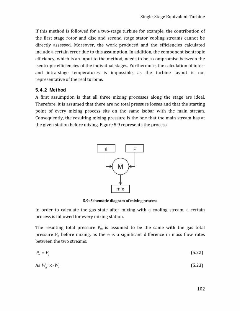
Single-Stage Equivalent Turbine
102
If this method is followed for a two-stage turbine for example, the contribution of the first stage rotor and disc and second stage stator cooling streams cannot be directly assessed. Moreover, the work produced and the efficiencies calculated include a certain error due to this assumption. In addition, the component isentropic efficiency, which is an input to the method, needs to be a compromise between the isentropic efficiencies of the individual stages. Furthermore, the calculation of inter- and intra-stage temperatures is impossible, as the turbine layout is not representative of the real turbine.
5.4.2 Method A first assumption is that all three mixing processes along the stage are ideal. Therefore, it is assumed that there are no total pressure losses and that the starting point of every mixing process sits on the same isobar with the main stream. Consequently, the resulting mixing pressure is the one that the main stream has at the given station before mixing. Figure 5.9 represents the process.
5.9: Schematic diagram of mixing process
In order to calculate the gas state after mixing with a cooling stream, a certain process is followed for every mixing station.
The resulting total pressure Pm is assumed to be the same with the gas total pressure Pg before mixing, as there is a significant difference in mass flow rates between the two streams:
m gP P= (5.22)
As g cW W>> (5.23)
Single-Stage Equivalent Turbine
103
The resulting mass flow after the mixing is the sum of the two individual mass flows of the gas and coolant:
m g cW W W= + (5.24)
The new fuel-to-air ratio can be calculated as following:
mm
W CFARC−
= (5.25)
Where
1 1g c
g c
W WCFAR FAR
= ++ +
(5.26)
With 0cFAR = (5.27)
Having the temperature and fuel-to-air ratio for gas and coolant, the heat capacity and enthalpy can be calculated for both:
( ), ,p g g gC f FAR T= (5.28)
And ( ), ,p c c cC f FAR T= (5.29)
And then:
,g p g gH C T= × (5.30)
And ,c p c cH C T= × (5.31)
And therefore, the enthalpy Hm after mixing is calculated as following:
g g c cm
m
H W H WH
W× + ×
= (5.32)
Finally, after following an iterative process, both Tm and Cp,m are determined, as following:
,/m m p mT H C= (5.33)

Single-Stage Equivalent Turbine
104
The widely used isentropic turbine efficiency is defined as following, which accounts just for the expansion process:
,
i ois
s is i s o
H HTW DHnTW DH H H
−= = =
− (5.34)
This is a figure indicative of the technology level of the device, but differs from the thermodynamic turbine efficiency, which is also affected by the amount and state of cooling air used. Again, the definition of the accounting system is important as a number of different efficiencies can be calculated. The last method updates, that include the mixing processes, enable the calculation of three new efficiency definitions.
First, the thermodynamic efficiency, which includes the contribution of all three cooling streams at the denominator, as they expand isentropically from their initial state to the final state at the turbine outlet, which is common for the gas and the three streams:
, , , , , , , , ,
ths
g is c Stator is c Stator c Rotor is c Rotor c Disc is c Disc
TWnTW
TWW DH W DH W DH W DH
= =
× + × + × + ×
(5.35)
The thermodynamic efficiency is an important figure, since is more indicative of the actual work potential of the turbine, including the cooling. It can significantly differ from the isentropic efficiency, as the amount of air used for cooling is a high proportion of the core mass flow rate.
Depending on the accounting system that someone may use, the amount of air used for the rotor and disc cooling may be included or not at the definition of the efficiency. This is because those streams have a certain work potential if expanded, but it is assumed that they do not contribute to the expansion process of a single-stage turbine. There is therefore an efficiency definition that does not count any stream after the turbine rotor, since they have a work potential that is not used in reality.
The definition of this efficiency follows:
Multistage Turbine
105
, , ,th
s g is c Stator is c Stator
TW TWnTW W DH W DH
= =× + ×
(5.36)
Again, the difference is a matter of definition of what an ideal expansion would be. There is no need for universal agreement, but a turbine designer should be aware of what is the definition used by a project partner and compare results on a common basis.
At this point, it is important to mention that in reality there may be different sources of loss accounted or not. To give some examples, the work required for the acceleration of the rotor coolant to the blade velocity may be accounted, the disc windage or the bearing losses. It is crucial to define accurately what an efficiency definition includes, and the same applies of course to the cooling streams accounted.
5.5 Multistage Turbine
5.5.1 Introduction The final step towards multi-stage turbine simulation is the introduction of a fully one-dimensional method, where every stage is simulated independently. This means that the processes along the turbine are represented by a number of stations, where every station corresponds to a certain process. The improvements over a zero-dimensional turbine or an equivalent single-stage are significant for physically two- or multi-stage turbines. The influence of every cooling stream is now addressed more realistically, at the cycle point where it actually happens.
This development enables the calculation of the three important figures, as set earlier in the chapter: First, the inter-stage and intra-stage temperatures along every blade row and cooling station. Second, the calculated turbine work is based on the enthalpy potential and mass flow of the gas and coolant mixture before every rotor. Third, the calculated thermodynamic efficiencies are based on the actual work and the enthalpy potential of every individual cooling stream, additionally to the main stream.
5.5.2 Method Going back to figure 5.6, the control volume has been further expanded, in order to include all the stages independently. For every stage and station, the mixing and expansion processes and calculations of paragraphs 5.3 and 5.4 are repeated and the outputs act as inputs for the stage(s) downstream. Therefore, for a two-stage turbine, there will be six mixing and two expansion processes in total, calculated in a
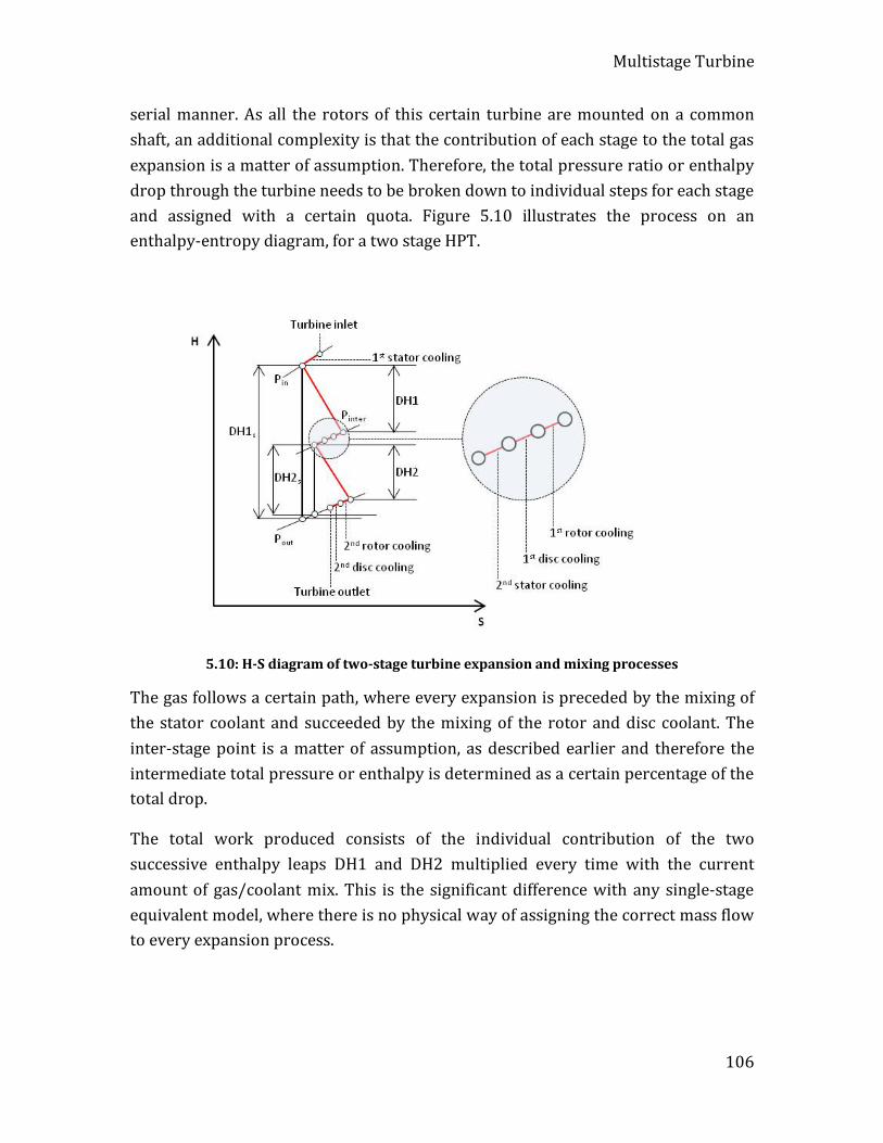
Multistage Turbine
106
serial manner. As all the rotors of this certain turbine are mounted on a common shaft, an additional complexity is that the contribution of each stage to the total gas expansion is a matter of assumption. Therefore, the total pressure ratio or enthalpy drop through the turbine needs to be broken down to individual steps for each stage and assigned with a certain quota. Figure 5.10 illustrates the process on an enthalpy-entropy diagram, for a two stage HPT.
5.10: H-S diagram of two-stage turbine expansion and mixing processes
The gas follows a certain path, where every expansion is preceded by the mixing of the stator coolant and succeeded by the mixing of the rotor and disc coolant. The inter-stage point is a matter of assumption, as described earlier and therefore the intermediate total pressure or enthalpy is determined as a certain percentage of the total drop.
The total work produced consists of the individual contribution of the two successive enthalpy leaps DH1 and DH2 multiplied every time with the current amount of gas/coolant mix. This is the significant difference with any single-stage equivalent model, where there is no physical way of assigning the correct mass flow to every expansion process.
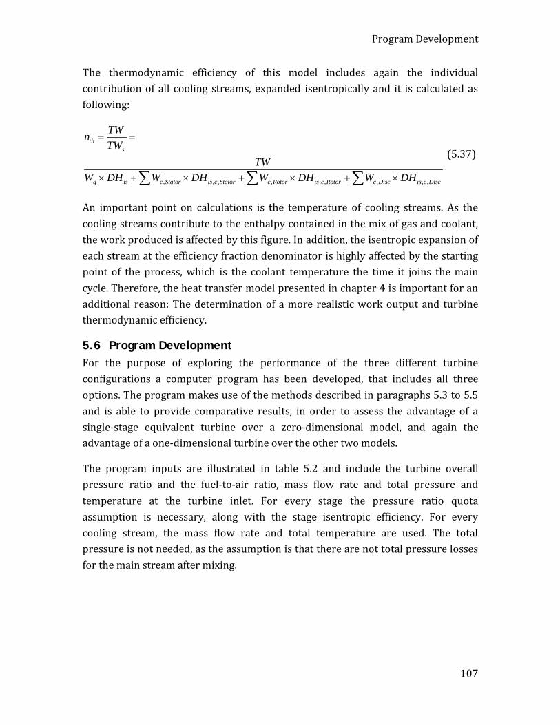
Program Development
107
The thermodynamic efficiency of this model includes again the individual contribution of all cooling streams, expanded isentropically and it is calculated as following:
, , , , , , , , ,
ths
g is c Stator is c Stator c Rotor is c Rotor c Disc is c Disc
TWnTW
TWW DH W DH W DH W DH
= =
× + × + × + ×∑ ∑ ∑
(5.37)
An important point on calculations is the temperature of cooling streams. As the cooling streams contribute to the enthalpy contained in the mix of gas and coolant, the work produced is affected by this figure. In addition, the isentropic expansion of each stream at the efficiency fraction denominator is highly affected by the starting point of the process, which is the coolant temperature the time it joins the main cycle. Therefore, the heat transfer model presented in chapter 4 is important for an additional reason: The determination of a more realistic work output and turbine thermodynamic efficiency.
5.6 Program Development For the purpose of exploring the performance of the three different turbine configurations a computer program has been developed, that includes all three options. The program makes use of the methods described in paragraphs 5.3 to 5.5 and is able to provide comparative results, in order to assess the advantage of a single-stage equivalent turbine over a zero-dimensional model, and again the advantage of a one-dimensional turbine over the other two models.
The program inputs are illustrated in table 5.2 and include the turbine overall pressure ratio and the fuel-to-air ratio, mass flow rate and total pressure and temperature at the turbine inlet. For every stage the pressure ratio quota assumption is necessary, along with the stage isentropic efficiency. For every cooling stream, the mass flow rate and total temperature are used. The total pressure is not needed, as the assumption is that there are not total pressure losses for the main stream after mixing.
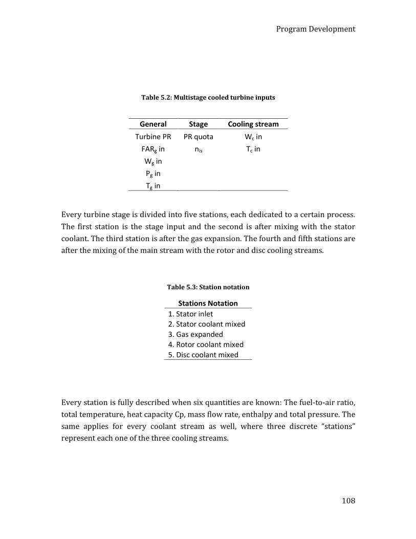
Program Development
108
Table 5.2: Multistage cooled turbine inputs
General Stage Cooling stream Turbine PR PR quota Wc in
FARg in nis Tc in Wg in
Pg in Tg in
Every turbine stage is divided into five stations, each dedicated to a certain process. The first station is the stage input and the second is after mixing with the stator coolant. The third station is after the gas expansion. The fourth and fifth stations are after the mixing of the main stream with the rotor and disc cooling streams.
Table 5.3: Station notation
Stations Notation 1. Stator inlet 2. Stator coolant mixed 3. Gas expanded 4. Rotor coolant mixed 5. Disc coolant mixed
Every station is fully described when six quantities are known: The fuel-to-air ratio, total temperature, heat capacity Cp, mass flow rate, enthalpy and total pressure. The same applies for every coolant stream as well, where three discrete “stations” represent each one of the three cooling streams.
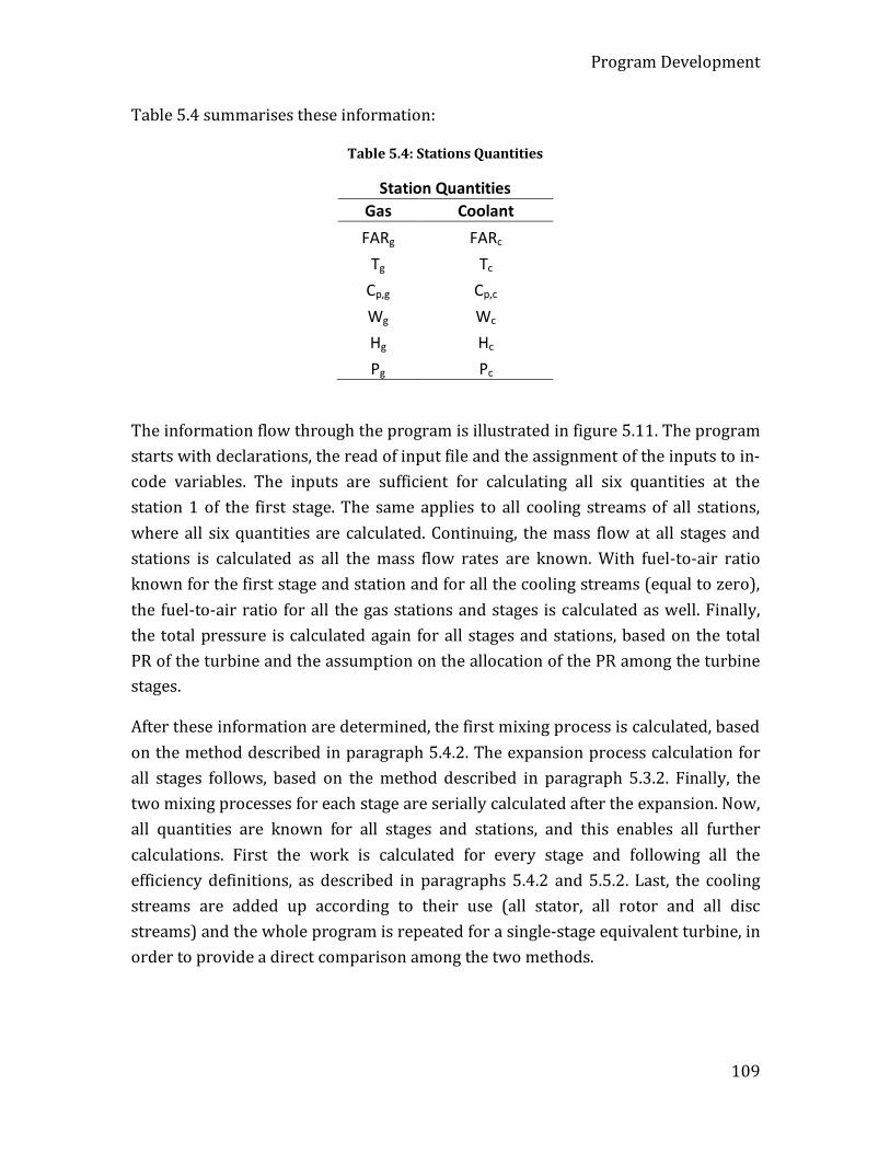
Program Development
109
Table 5.4 summarises these information:
Table 5.4: Stations Quantities
Station Quantities Gas Coolant FARg FARc
Tg Tc Cp,g Cp,c Wg Wc Hg Hc Pg Pc
The information flow through the program is illustrated in figure 5.11. The program starts with declarations, the read of input file and the assignment of the inputs to in-code variables. The inputs are sufficient for calculating all six quantities at the station 1 of the first stage. The same applies to all cooling streams of all stations, where all six quantities are calculated. Continuing, the mass flow at all stages and stations is calculated as all the mass flow rates are known. With fuel-to-air ratio known for the first stage and station and for all the cooling streams (equal to zero), the fuel-to-air ratio for all the gas stations and stages is calculated as well. Finally, the total pressure is calculated again for all stages and stations, based on the total PR of the turbine and the assumption on the allocation of the PR among the turbine stages.
After these information are determined, the first mixing process is calculated, based on the method described in paragraph 5.4.2. The expansion process calculation for all stages follows, based on the method described in paragraph 5.3.2. Finally, the two mixing processes for each stage are serially calculated after the expansion. Now, all quantities are known for all stages and stations, and this enables all further calculations. First the work is calculated for every stage and following all the efficiency definitions, as described in paragraphs 5.4.2 and 5.5.2. Last, the cooling streams are added up according to their use (all stator, all rotor and all disc streams) and the whole program is repeated for a single-stage equivalent turbine, in order to provide a direct comparison among the two methods.
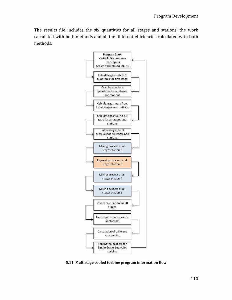
Program Development
110
The results file includes the six quantities for all stages and stations, the work calculated with both methods and all the different efficiencies calculated with both methods.
5.11: Multistage cooled turbine program information flow
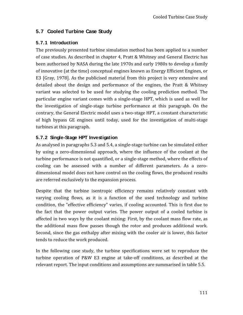
Cooled Turbine Case Study
111
5.7 Cooled Turbine Case Study
5.7.1 Introduction The previously presented turbine simulation method has been applied to a number of case studies. As described in chapter 4, Pratt & Whitney and General Electric has been authorised by NASA during the late 1970s and early 1980s to develop a family of innovative (at the time) conceptual engines known as Energy Efficient Engines, or E3 [Gray, 1978]. As the publicised material from this project is very extensive and detailed about the design and performance of the engines, the Pratt & Whitney variant was selected to be used for studying the cooling prediction method. The particular engine variant comes with a single-stage HPT, which is used as well for the investigation of single-stage turbine performance at this paragraph. On the contrary, the General Electric model uses a two-stage HPT, a constant characteristic of high bypass GE engines until today, used for the investigation of multi-stage turbines at this paragraph.
5.7.2 Single-Stage HPT Investigation As analysed in paragraphs 5.3 and 5.4, a single-stage turbine can be simulated either by using a zero-dimensional approach, where the influence of the coolant at the turbine performance is not quantified, or a single-stage method, where the effects of cooling can be assessed with a number of different parameters. As a zero-dimensional model does not have control on the cooling flows, the produced results are referred exclusively to the expansion process.
Despite that the turbine isentropic efficiency remains relatively constant with varying cooling flows, as it is a function of the used technology and turbine condition, the “effective efficiency” varies, if cooling accounted. This is first due to the fact that the power output varies. The power output of a cooled turbine is affected in two ways by the coolant mixing: First, by the coolant mass flow rate, as the additional mass flow passes though the rotor and produces additional work. Second, since the gas enthalpy after mixing with the cooler air is lower, this factor tends to reduce the work produced.
In the following case study, the turbine specifications were set to reproduce the turbine operation of P&W E3 engine at take-off conditions, as described at the relevant report. The input conditions and assumptions are summarised in table 5.5.
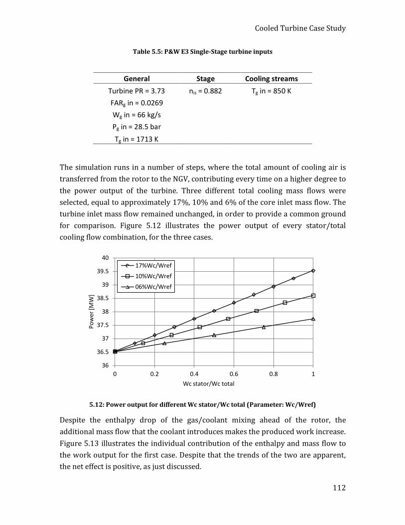
Cooled Turbine Case Study
112
Table 5.5: P&W E3 Single-Stage turbine inputs
General Stage Cooling streams Turbine PR = 3.73 nis = 0.882 Tg in = 850 K FARg in = 0.0269
Wg in = 66 kg/s Pg in = 28.5 bar Tg in = 1713 K
The simulation runs in a number of steps, where the total amount of cooling air is transferred from the rotor to the NGV, contributing every time on a higher degree to the power output of the turbine. Three different total cooling mass flows were selected, equal to approximately 17%, 10% and 6% of the core inlet mass flow. The turbine inlet mass flow remained unchanged, in order to provide a common ground for comparison. Figure 5.12 illustrates the power output of every stator/total cooling flow combination, for the three cases.
5.12: Power output for different Wc stator/Wc total (Parameter: Wc/Wref)
Despite the enthalpy drop of the gas/coolant mixing ahead of the rotor, the additional mass flow that the coolant introduces makes the produced work increase. Figure 5.13 illustrates the individual contribution of the enthalpy and mass flow to the work output for the first case. Despite that the trends of the two are apparent, the net effect is positive, as just discussed.
36
36.5
37
37.5
38
38.5
39
39.5
40
0 0.2 0.4 0.6 0.8 1
Pow
er [M
W]
Wc stator/Wc total
17%Wc/Wref
10%Wc/Wref
06%Wc/Wref
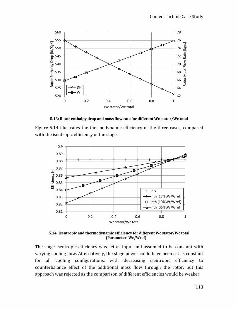
Cooled Turbine Case Study
113
5.13: Rotor enthalpy drop and mass flow rate for different Wc stator/Wc total
Figure 5.14 illustrates the thermodynamic efficiency of the three cases, compared with the isentropic efficiency of the stage.
5.14: Isentropic and thermodynamic efficiency for different Wc stator/Wc total (Parameter: Wc/Wref)
The stage isentropic efficiency was set as input and assumed to be constant with varying cooling flow. Alternatively, the stage power could have been set as constant for all cooling configurations, with decreasing isentropic efficiency to counterbalance effect of the additional mass flow through the rotor, but this approach was rejected as the comparison of different efficiencies would be weaker.
62
64
66
68
70
72
74
76
78
520
525
530
535
540
545
550
555
560
0 0.2 0.4 0.6 0.8 1
Roto
r Mas
s Flo
w R
ate
[kg/
s]
Roto
r Ent
halp
y Dr
op [k
J/Kg
K]
Wc stator/Wc total
DH W
0.81
0.82
0.83
0.84
0.85
0.86
0.87
0.88
0.89
0.9
0 0.2 0.4 0.6 0.8 1
Effic
ienc
y [-]
Wc stator/Wc total
nis nth [17%Wc/Wref] nth [10%Wc/Wref] nth [06%Wc/Wref]

Cooled Turbine Case Study
114
The thermodynamic efficiency, which includes the contribution of all cooling flows, starts from a low level, as the rotor flow does not contribute to the work produced, but accounted as potential source of work. The difference among the three cases for 0% stator cooling is significant. The work output of the three is identical, as illustrated in figure 5.12, but the work potential of the cooling flow directed to the rotor is higher for the case where Wc/Wref=17%. Therefore, the thermodynamic efficiency of the latter is lower. While cooling flow is passing from rotor to stator, the additional mass starts contributing to the work produced, despite the decreased enthalpy discussed earlier. The increased work starts improving the efficiency, since the denominator remains constant, as the work potential of all the flows remains unchanged.
The efficiency keeps increasing until equals the isentropic efficiency of the stage at a certain point, common for all three cases. At this point, the following happens:
1 ,
2 2 3 2 2 3
2 2 3 1 1 , 1
2 2 3 1 1 , 1
( ) ( )( ) ( ) ( )
( ) ( ) ( )
is th
is is c is c
is is c is c is
is is c is c is
n n
TW TWTW W DH W DH
W H H W H HW H H W H H W H H
W H H W H H W H H
=
⇒ =× + ×
− −⇒ =
− × − + × −
⇒ − = × − + × −
(5.38)
As the right side of the equation remains constant along the cooling air redistribution between the rotor and stator, it is the left side of the equation that equals it at a specific point. One could expect the two sides of the equation to be equal at the point where 100% of coolant is directed to stator, as at this point the amount of gas or air on the left side equals the total one on the right side. This is not the case, as the sum of the work produced by individual ideal expansions of gas and air is not the same as the ideal expansion of the mix composed of the two portions, and this is because of the deviation of the isobars at the enthalpy-entropy diagram. Therefore, the closer the coolant to the gas temperature it is, the further right is the point where the two efficiencies concur.
Another remark is that this point is the same for the three cases. As for every case and at this exact point the coolant contributes with the same proportion at the left
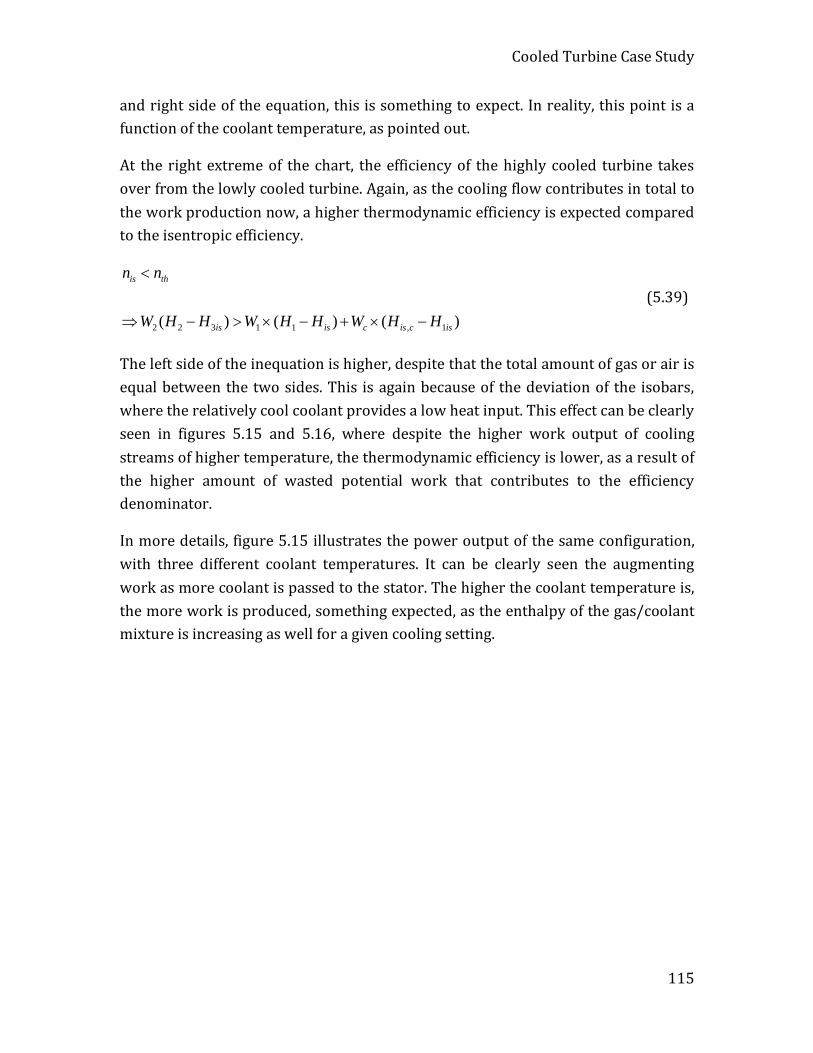
Cooled Turbine Case Study
115
and right side of the equation, this is something to expect. In reality, this point is a function of the coolant temperature, as pointed out.
At the right extreme of the chart, the efficiency of the highly cooled turbine takes over from the lowly cooled turbine. Again, as the cooling flow contributes in total to the work production now, a higher thermodynamic efficiency is expected compared to the isentropic efficiency.
2 2 3 1 1 , 1( ) ( ) ( )
is th
is is c is c is
n n
W H H W H H W H H
<
⇒ − > × − + × − (5.39)
The left side of the inequation is higher, despite that the total amount of gas or air is equal between the two sides. This is again because of the deviation of the isobars, where the relatively cool coolant provides a low heat input. This effect can be clearly seen in figures 5.15 and 5.16, where despite the higher work output of cooling streams of higher temperature, the thermodynamic efficiency is lower, as a result of the higher amount of wasted potential work that contributes to the efficiency denominator.
In more details, figure 5.15 illustrates the power output of the same configuration, with three different coolant temperatures. It can be clearly seen the augmenting work as more coolant is passed to the stator. The higher the coolant temperature is, the more work is produced, something expected, as the enthalpy of the gas/coolant mixture is increasing as well for a given cooling setting.

Cooled Turbine Case Study
116
5.15: Power output for different Wc stator/Wc total (Parameter: Tc)
Despite the increased shaft output, the effect in thermodynamic efficiency is the opposite: Efficiency decreases with increasing coolant temperature, since apart from the increasing power, the ideal work potential of the cooling streams increases as well, at a higher degree with increasing temperature. This can be observed in figure 5.16, where the closer the coolant is to the gas temperature, the more cooling mass at the stator is needed to match the stage isentropic efficiency. It is interesting to mention again that the point where the two efficiencies intersect is a function of the coolant temperature and not the total amount of cooling air used.
36
36.5
37
37.5
38
38.5
39
0 0.2 0.4 0.6 0.8 1
Pow
er [M
W]
Wc stator/Wc total
Tc=850K
Tc=1075K
Tc=1300K
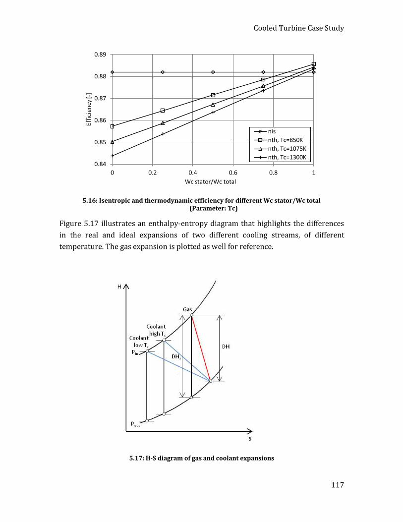
Cooled Turbine Case Study
117
5.16: Isentropic and thermodynamic efficiency for different Wc stator/Wc total (Parameter: Tc)
Figure 5.17 illustrates an enthalpy-entropy diagram that highlights the differences in the real and ideal expansions of two different cooling streams, of different temperature. The gas expansion is plotted as well for reference.
5.17: H-S diagram of gas and coolant expansions
0.84
0.85
0.86
0.87
0.88
0.89
0 0.2 0.4 0.6 0.8 1
Effic
ienc
y [-]
Wc stator/Wc total
nis nth, Tc=850K nth, Tc=1075K nth, Tc=1300K

Cooled Turbine Case Study
118
By keeping a certain level of cooling air distributed between the stator and rotor and adjusting the coolant temperature, figure 5.18 results. The effect of a varying coolant temperature at the thermodynamic efficiency is illustrated for three different stator/total cooling distributions, compared with the stage isentropic efficiency. Again, the higher proportion of cooling directed to stator is, the higher the efficiency. It is important to notice that along a line the efficiency drops with higher coolant temperature, as explained earlier and attributed to the isobars deviation. Another interesting remark is that for a lower stator/total air distribution the line gets steeper. This is because the contribution of the rotor coolant becomes more dominant at the thermodynamic efficiency calculation as a higher amount of air is directed towards it.
5.18: Isentropic and thermodynamic efficiency for different Tc (Parameter: Wc stator/Wc total)
Figure 5.19 illustrates a comparison between the isentropic, the thermodynamic and the second definition for the thermodynamic efficiency as presented in paragraph 5.4.2. According to the second definition, the contribution of the rotor and disc cooling flows is not accounted to the ideal work at the denominator of the efficiency definition. This is not wrong, but it generally depends on the bookkeeping system of a designer. Someone may argue that the rotor and disc flows are not contributing to work anyway and there is no need to be accounted. On the other hand, someone may say that as their potential work is wasted, this should be acknowledged in the turbine performance figures as well, apart from the engine thermal efficiency.
0.865
0.869
0.873
0.877
0.881
0.885
0.889
800 900 1000 1100 1200 1300 1400
Effic
ienc
y [-]
Coolant Temperature (K)
n is nth, 75% stator c nth, 87.5% stator c nth, 100% stator c
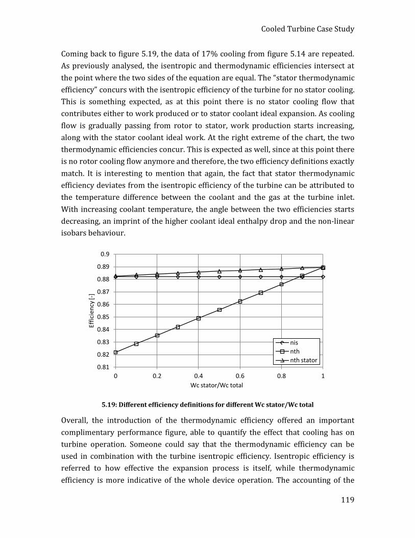
Cooled Turbine Case Study
119
Coming back to figure 5.19, the data of 17% cooling from figure 5.14 are repeated. As previously analysed, the isentropic and thermodynamic efficiencies intersect at the point where the two sides of the equation are equal. The “stator thermodynamic efficiency” concurs with the isentropic efficiency of the turbine for no stator cooling. This is something expected, as at this point there is no stator cooling flow that contributes either to work produced or to stator coolant ideal expansion. As cooling flow is gradually passing from rotor to stator, work production starts increasing, along with the stator coolant ideal work. At the right extreme of the chart, the two thermodynamic efficiencies concur. This is expected as well, since at this point there is no rotor cooling flow anymore and therefore, the two efficiency definitions exactly match. It is interesting to mention that again, the fact that stator thermodynamic efficiency deviates from the isentropic efficiency of the turbine can be attributed to the temperature difference between the coolant and the gas at the turbine inlet. With increasing coolant temperature, the angle between the two efficiencies starts decreasing, an imprint of the higher coolant ideal enthalpy drop and the non-linear isobars behaviour.
5.19: Different efficiency definitions for different Wc stator/Wc total
Overall, the introduction of the thermodynamic efficiency offered an important complimentary performance figure, able to quantify the effect that cooling has on turbine operation. Someone could say that the thermodynamic efficiency can be used in combination with the turbine isentropic efficiency. Isentropic efficiency is referred to how effective the expansion process is itself, while thermodynamic efficiency is more indicative of the whole device operation. The accounting of the
0.81
0.82
0.83
0.84
0.85
0.86
0.87
0.88
0.89
0.9
0 0.2 0.4 0.6 0.8 1
Effic
ienc
y [-]
Wc stator/Wc total
nis nth nth stator
Cooled Turbine Case Study
120
cooling streams is essential towards this direction and this is the main reason that all cooling flows have to be included to the turbine model, in contrast with a zero-dimensional model.
5.7.3 Two-Stage HPT Investigation A second set of simulations has been executed for the case of a two-stage virtual turbine. The simulations use as an engine model based on the performance of the General Electric variant of the E3 engine [NASA, 1980a] [NASA, 1980b], [NASA, 1982]. The results of the multi-stage model will be assessed based on three criteria:
• The ability to provide intra- and inter-stage temperatures • The turbine work prediction • The different calculated efficiencies
The results will be compared as well against corresponding results obtained with the use of a single-stage equivalent model of the engine turbine.
As now more than one stages contribute to the expansion process, an important point is the way that isentropic efficiency is communicated to the user. As explained earlier, despite the fact that isentropic efficiency has been the standard figure in industry to communicate the technology involved at the gas expansion process, this figure needs to be used with caution on what represents and what is the effect on the thermodynamic efficiency of a multi-stage turbine.
In the case of a physically single-stage HPT, the isentropic efficiency of the stage matches the isentropic efficiency of the turbine. In the case of a multi-stage turbine though, the isentropic efficiency of the individual stages does not match the one of the turbine, again, because of the fact that the pressure lines deviate at the enthalpy-entropy diagram. The polytropic efficiency is a much more indicative way of defining the technology involved, as it remains the same for all expansions involved.
The main effects of this assumption are three:
• First, the isentropic efficiency of the two or more individual expansions does not match with the isentropic efficiency of a single expansion between the two pressure boundaries of the turbine.
• Second, the assumption of inter-stage pressure quotas has an effect on the isentropic efficiency, or inversely to the work delivered, as the isentropic efficiency is an input at this particular case.
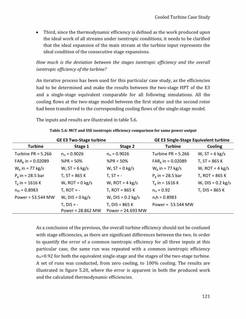
Cooled Turbine Case Study
121
• Third, since the thermodynamic efficiency is defined as the work produced upon the ideal work of all streams under isentropic conditions, it needs to be clarified that the ideal expansion of the main stream at the turbine input represents the ideal condition of the consecutive stage expansions.
How much is the deviation between the stages isentropic efficiency and the overall isentropic efficiency of the turbine?
An iterative process has been used for this particular case study, as the efficiencies had to be determined and make the results between the two-stage HPT of the E3 and a single-stage equivalent comparable for all following simulations. All the cooling flows at the two-stage model between the first stator and the second rotor had been transferred to the corresponding cooling flows of the single-stage model.
The inputs and results are illustrated in table 5.6.
Table 5.6: MCT and SSE isentropic efficiency comparison for same power output
GE E3 Two-Stage turbine GE E3 Single-Stage Equivalent turbine Turbine Stage 1 Stage 2 Turbine Cooling
Turbine PR = 5.266 nis = 0.9026 nis = 0.9026 Turbine PR = 5.266 Wc ST = 6 kg/s FARg in = 0.02089 %PR = 50% %PR = 50% FARg in = 0.02089 Tc ST = 865 K Wg in = 77 kg/s Wc ST = 6 kg/s Wc ST = 0 kg/s Wg in = 77 kg/s Wc ROT = 4 kg/s Pg in = 28.5 bar Tc ST = 865 K Tc ST = - Pg in = 28.5 bar Tc ROT = 865 K Tg in = 1616 K Wc ROT = 0 kg/s Wc ROT = 4 kg/s Tg in = 1616 K Wc DIS = 0.2 kg/s nth = 0.8983 Tc ROT = - Tc ROT = 865 K nis = 0.92 Tc DIS = 865 K Power = 53.544 MW Wc DIS = 0 kg/s Wc DIS = 0.2 kg/s nth = 0.8983
Tc DIS = - Tc DIS = 865 K Power = 53.544 MW Power = 28.862 MW Power = 24.693 MW
As a conclusion of the previous, the overall turbine efficiency should not be confused with stage efficiencies, as there are significant differences between the two. In order to quantify the error of a common isentropic efficiency for all three inputs at this particular case, the same run was repeated with a common isentropic efficiency nis=0.92 for both the equivalent single-stage and the stages of the two-stage turbine. A set of runs was conducted, from zero cooling, to 100% cooling. The results are illustrated in figure 5.20, where the error is apparent in both the produced work and the calculated thermodynamic efficiencies.
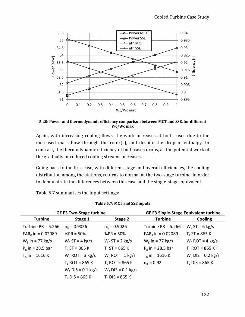
Cooled Turbine Case Study
122
5.20: Power and thermodynamic efficiency comparison between MCT and SSE, for different Wc/Wc max
Again, with increasing cooling flows, the work increases at both cases due to the increased mass flow through the rotor(s), and despite the drop in enthalpy. In contrast, the thermodynamic efficiency of both cases drops, as the potential work of the gradually introduced cooling streams increases.
Going back to the first case, with different stage and overall efficiencies, the cooling distribution among the stations, returns to normal at the two-stage turbine, in order to demonstrate the differences between this case and the single-stage equivalent.
Table 5.7 summarises the input settings:
Table 5.7: MCT and SSE inputs
GE E3 Two-Stage turbine GE E3 Single-Stage Equivalent turbine Turbine Stage 1 Stage 2 Turbine Cooling
Turbine PR = 5.266 nis = 0.9026 nis = 0.9026 Turbine PR = 5.266 Wc ST = 6 kg/s FARg in = 0.02089 %PR = 50% %PR = 50% FARg in = 0.02089 Tc ST = 865 K Wg in = 77 kg/s Wc ST = 4 kg/s Wc ST = 2 kg/s Wg in = 77 kg/s Wc ROT = 4 kg/s Pg in = 28.5 bar Tc ST = 865 K Tc ST = 865 K Pg in = 28.5 bar Tc ROT = 865 K Tg in = 1616 K Wc ROT = 3 kg/s Wc ROT = 1 kg/s Tg in = 1616 K Wc DIS = 0.2 kg/s
Tc ROT = 865 K Tc ROT = 865 K nis = 0.92 Tc DIS = 865 K
Wc DIS = 0.1 kg/s Wc DIS = 0.1 kg/s
Tc DIS = 865 K Tc DIS = 865 K
0.895
0.9
0.905
0.91
0.915
0.92
0.925
0.93
0.935
0.94
51
51.5
52
52.5
53
53.5
54
54.5
55
55.5
0 0.1 0.2 0.3 0.4 0.5 0.6 0.7 0.8 0.9 1
Effic
ienc
y [-]
Pow
er [M
W]
Wc/Wc max
Power MCT Power SSE nth MCT nth SSE
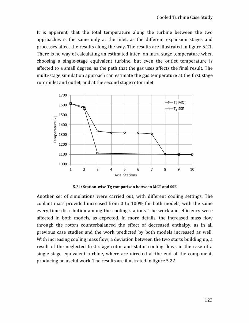
Cooled Turbine Case Study
123
It is apparent, that the total temperature along the turbine between the two approaches is the same only at the inlet, as the different expansion stages and processes affect the results along the way. The results are illustrated in figure 5.21. There is no way of calculating an estimated inter- on intra-stage temperature when choosing a single-stage equivalent turbine, but even the outlet temperature is affected to a small degree, as the path that the gas uses affects the final result. The multi-stage simulation approach can estimate the gas temperature at the first stage rotor inlet and outlet, and at the second stage rotor inlet.
5.21: Station-wise Tg comparison between MCT and SSE
Another set of simulations were carried out, with different cooling settings. The coolant mass provided increased from 0 to 100% for both models, with the same every time distribution among the cooling stations. The work and efficiency were affected in both models, as expected. In more details, the increased mass flow through the rotors counterbalanced the effect of decreased enthalpy, as in all previous case studies and the work predicted by both models increased as well. With increasing cooling mass flow, a deviation between the two starts building up, a result of the neglected first stage rotor and stator cooling flows in the case of a single-stage equivalent turbine, where are directed at the end of the component, producing no useful work. The results are illustrated in figure 5.22.
1000
1100
1200
1300
1400
1500
1600
1700
1 2 3 4 5 6 7 8 9 10
Tem
pera
ture
[k]
Axial Stations
Tg MCT Tg SSE
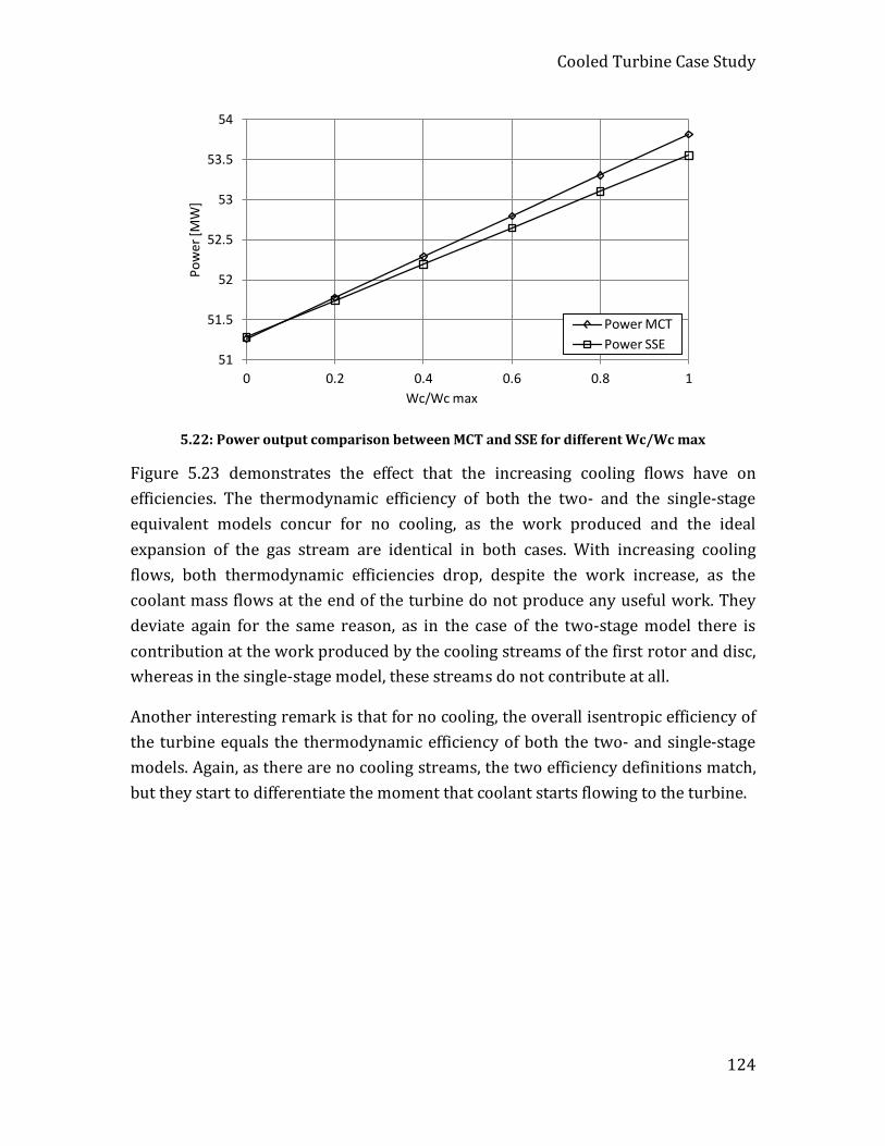
Cooled Turbine Case Study
124
5.22: Power output comparison between MCT and SSE for different Wc/Wc max
Figure 5.23 demonstrates the effect that the increasing cooling flows have on efficiencies. The thermodynamic efficiency of both the two- and the single-stage equivalent models concur for no cooling, as the work produced and the ideal expansion of the gas stream are identical in both cases. With increasing cooling flows, both thermodynamic efficiencies drop, despite the work increase, as the coolant mass flows at the end of the turbine do not produce any useful work. They deviate again for the same reason, as in the case of the two-stage model there is contribution at the work produced by the cooling streams of the first rotor and disc, whereas in the single-stage model, these streams do not contribute at all.
Another interesting remark is that for no cooling, the overall isentropic efficiency of the turbine equals the thermodynamic efficiency of both the two- and single-stage models. Again, as there are no cooling streams, the two efficiency definitions match, but they start to differentiate the moment that coolant starts flowing to the turbine.
51
51.5
52
52.5
53
53.5
54
0 0.2 0.4 0.6 0.8 1
Pow
er [M
W]
Wc/Wc max
Power MCT Power SSE
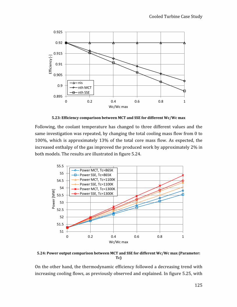
Cooled Turbine Case Study
125
5.23: Efficiency comparison between MCT and SSE for different Wc/Wc max
Following, the coolant temperature has changed to three different values and the same investigation was repeated, by changing the total cooling mass flow from 0 to 100%, which is approximately 13% of the total core mass flow. As expected, the increased enthalpy of the gas improved the produced work by approximately 2% in both models. The results are illustrated in figure 5.24.
5.24: Power output comparison between MCT and SSE for different Wc/Wc max (Parameter: Tc)
On the other hand, the thermodynamic efficiency followed a decreasing trend with increasing cooling flows, as previously observed and explained. In figure 5.25, with
0.895
0.9
0.905
0.91
0.915
0.92
0.925
0 0.2 0.4 0.6 0.8 1
Effic
ienc
y [-]
Wc/Wc max
nis nth MCT nth SSE
51
51.5
52
52.5
53
53.5
54
54.5
55
55.5
0 0.2 0.4 0.6 0.8 1
Pow
er [M
W]
Wc/Wc max
Power MCT, Tc=865K Power SSE, Tc=865K Power MCT, Tc=1100K Power SSE, Tc=1100K Power MCT, Tc=1300K Power SSE, Tc=1300K

Cooled Turbine Case Study
126
increasing coolant temperature, the efficiency drops, as expected and observed in paragraph 5.7.2 as well. This is a result of the greater work potential that the higher temperature cooling flows include. Part of this potential is directed to produce the increased actual work, but not all of it is utilised. The rest of it is just included to the flows that do not produce work and exits the turbine, having influenced the gas mass flow. This is the reason as well that the single-stage equivalent model is characterised by a lower efficiency as well, as a lower portion of the cooling air is used for useful work and a higher is just accounted as untapped. The difference between the two methods tends to increase with increasing temperature, as the work potential of hotter streams is higher, due to the non-linear behaviour of the gas properties.
5.25: Thermodynamic efficiency comparison between MCT and SSE for different Wc/Wc max (Parameter: Tc)
In figure 4.26, the effect of the coolant temperature in performance was investigated to the same range of coolant temperatures for three different cooling configurations, at the 50%, 75% and 100% of the maximum (approximately 6.5%, 9.5% and 13% of the total core mass flow). As expected, the thermodynamic efficiency for every case and model drops with increasing cooling mass flow and coolant temperature. The efficiency lines deviate though, as explained, due to the changing gas properties with varying temperature. The difference between the two models increases as well with increasing temperature for the same reason. The work potential of a higher temperature coolant increases as well. A part of this increase is translated into work
0.88
0.885
0.89
0.895
0.9
0.905
0.91
0.915
0.92
0.925
0 0.2 0.4 0.6 0.8 1
Effic
ienc
y [-]
Wc/Wc max
n is nth MCT, Tc=865K nth SSE, Tc=865K nth MCT, Tc=1100K nth SSE, Tc=1100K nth MCT, Tc=1300K
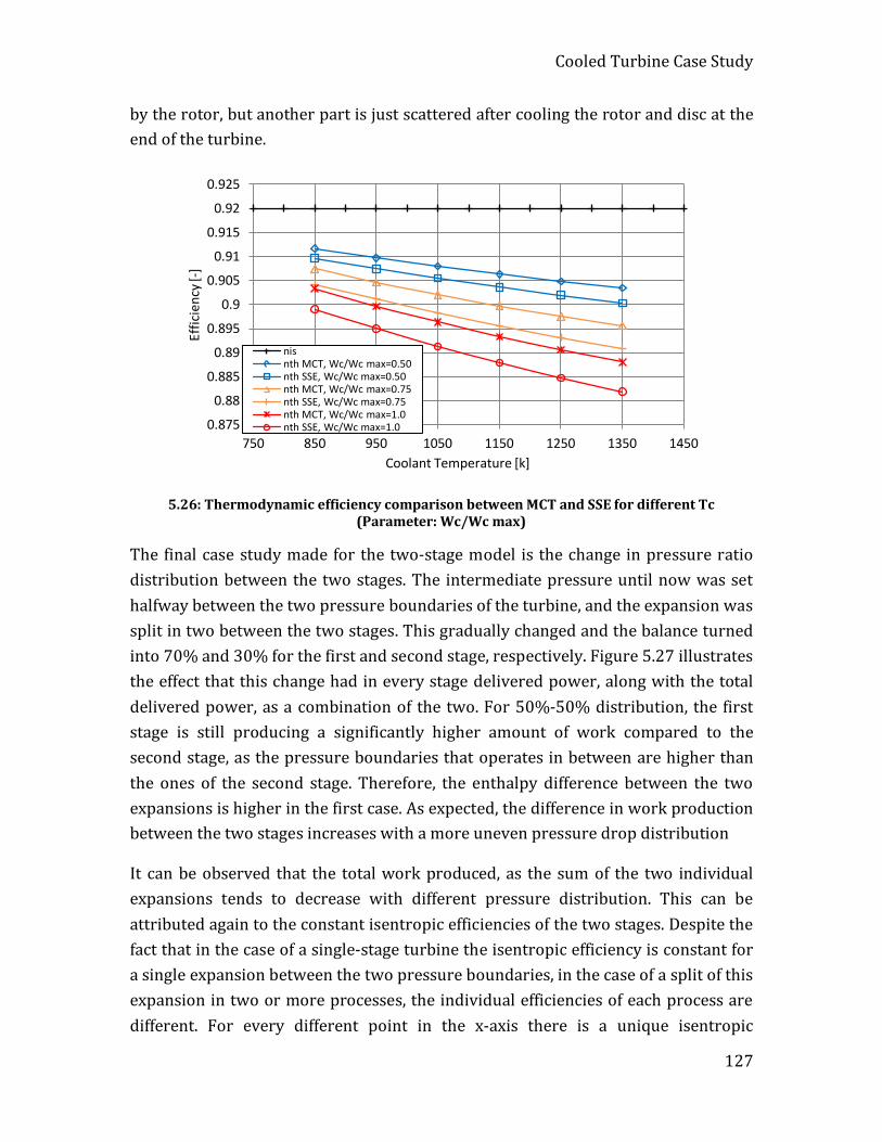
Cooled Turbine Case Study
127
by the rotor, but another part is just scattered after cooling the rotor and disc at the end of the turbine.
5.26: Thermodynamic efficiency comparison between MCT and SSE for different Tc (Parameter: Wc/Wc max)
The final case study made for the two-stage model is the change in pressure ratio distribution between the two stages. The intermediate pressure until now was set halfway between the two pressure boundaries of the turbine, and the expansion was split in two between the two stages. This gradually changed and the balance turned into 70% and 30% for the first and second stage, respectively. Figure 5.27 illustrates the effect that this change had in every stage delivered power, along with the total delivered power, as a combination of the two. For 50%-50% distribution, the first stage is still producing a significantly higher amount of work compared to the second stage, as the pressure boundaries that operates in between are higher than the ones of the second stage. Therefore, the enthalpy difference between the two expansions is higher in the first case. As expected, the difference in work production between the two stages increases with a more uneven pressure drop distribution
It can be observed that the total work produced, as the sum of the two individual expansions tends to decrease with different pressure distribution. This can be attributed again to the constant isentropic efficiencies of the two stages. Despite the fact that in the case of a single-stage turbine the isentropic efficiency is constant for a single expansion between the two pressure boundaries, in the case of a split of this expansion in two or more processes, the individual efficiencies of each process are different. For every different point in the x-axis there is a unique isentropic
0.875
0.88
0.885
0.89
0.895
0.9
0.905
0.91
0.915
0.92
0.925
750 850 950 1050 1150 1250 1350 1450
Effic
ienc
y [-]
Coolant Temperature [k]
nis nth MCT, Wc/Wc max=0.50 nth SSE, Wc/Wc max=0.50 nth MCT, Wc/Wc max=0.75 nth SSE, Wc/Wc max=0.75 nth MCT, Wc/Wc max=1.0 nth SSE, Wc/Wc max=1.0
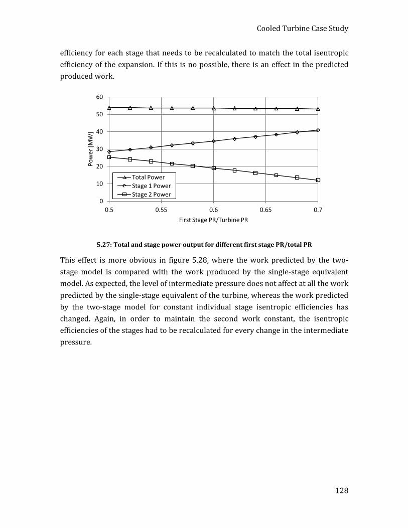
Cooled Turbine Case Study
128
efficiency for each stage that needs to be recalculated to match the total isentropic efficiency of the expansion. If this is no possible, there is an effect in the predicted produced work.
5.27: Total and stage power output for different first stage PR/total PR
This effect is more obvious in figure 5.28, where the work predicted by the two-stage model is compared with the work produced by the single-stage equivalent model. As expected, the level of intermediate pressure does not affect at all the work predicted by the single-stage equivalent of the turbine, whereas the work predicted by the two-stage model for constant individual stage isentropic efficiencies has changed. Again, in order to maintain the second work constant, the isentropic efficiencies of the stages had to be recalculated for every change in the intermediate pressure.
0
10
20
30
40
50
60
0.5 0.55 0.6 0.65 0.7
Pow
er [M
W]
First Stage PR/Turbine PR
Total Power Stage 1 Power Stage 2 Power
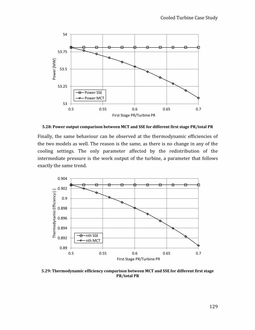
Cooled Turbine Case Study
129
5.28: Power output comparison between MCT and SSE for different first stage PR/total PR
Finally, the same behaviour can be observed at the thermodynamic efficiencies of the two models as well. The reason is the same, as there is no change in any of the cooling settings. The only parameter affected by the redistribution of the intermediate pressure is the work output of the turbine, a parameter that follows exactly the same trend.
5.29: Thermodynamic efficiency comparison between MCT and SSE for different first stage PR/total PR
53
53.25
53.5
53.75
54
0.5 0.55 0.6 0.65 0.7
Pow
er [M
W]
First Stage PR/Turbine PR
Power SSE Power MCT
0.89
0.892
0.894
0.896
0.898
0.9
0.902
0.904
0.5 0.55 0.6 0.65 0.7
Ther
mod
ynam
ic E
ffici
ency
[-]
First Stage PR/Turbine PR
nth SSE nth MCT
Cooled Turbine Case Study
130
5.7.4 Conclusions A comparison has been conducted among a zero-dimensional, a single-stage equivalent and a two-stage cooled turbine model. The complexity of the model increases to a certain degree with every one of the two upgrades, but there are significant benefits associated with them. In general, a zero-dimensional model does not account three main figures: The temperatures inside the turbine, the work produced by certain cooling streams and the thermodynamic efficiency.
In case that any gas temperature estimation between the inlet and the outlet of the turbine is needed, the utilisation of a model with the actual number of stages is necessary. In this particular scenario there is no alternative that can provide even a rough prediction of the external temperatures encountered by the blades and vanes, mainly for life prediction purposes. Therefore, the multi-stage model presented or a similar one is the only way to proceed.
As presented, the work produced by the cooling streams that join the main cycle after the first and before the last rotor can be important to a certain degree and affect the results. The benefit from a multi-stage approach is important only when the coolant temperature is relatively high and the amount of total cooling to the turbine is significant; at take-off conditions for instance.
The introduction of thermodynamic efficiency is an important additional feature that zero-dimensional modelling is not offering. It is important for a number of reasons: First, the thermodynamic efficiency is an indicative figure of how efficiently a cooled turbine operates in total and not just an indication of how effective the expansion process is. It cannot be a substance for the isentropic efficiency, since it is based on it, but it can work complementary. As the turbine efficiency can be defined in different ways, every type of turbine efficiency expresses different aspects of the turbine operation. Thus, there should be a clear definition of the actual performance aspects that they contribute to the efficiency calculation when a design team communicates results with another part. Overall, the isentropic efficiency should be used with caution as well, especially when referred to multi-stage turbines, where the stage intervals are dominant on the results.
Table 5.8 summarises the additional performance figures possible to be calculated with each methodology.
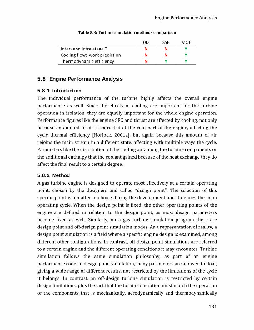
Engine Performance Analysis
131
Table 5.8: Turbine simulation methods comparison
0D SSE MCT Inter- and intra-stage T N N Y Cooling flows work prediction N N Y Thermodynamic efficiency N Y Y
5.8 Engine Performance Analysis
5.8.1 Introduction The individual performance of the turbine highly affects the overall engine performance as well. Since the effects of cooling are important for the turbine operation in isolation, they are equally important for the whole engine operation. Performance figures like the engine SFC and thrust are affected by cooling, not only because an amount of air is extracted at the cold part of the engine, affecting the cycle thermal efficiency [Horlock, 2001a], but again because this amount of air rejoins the main stream in a different state, affecting with multiple ways the cycle. Parameters like the distribution of the cooling air among the turbine components or the additional enthalpy that the coolant gained because of the heat exchange they do affect the final result to a certain degree.
5.8.2 Method A gas turbine engine is designed to operate most effectively at a certain operating point, chosen by the designers and called “design point”. The selection of this specific point is a matter of choice during the development and it defines the main operating cycle. When the design point is fixed, the other operating points of the engine are defined in relation to the design point, as most design parameters become fixed as well. Similarly, on a gas turbine simulation program there are design point and off-design point simulation modes. As a representation of reality, a design point simulation is a field where a specific engine design is examined, among different other configurations. In contrast, off-design point simulations are referred to a certain engine and the different operating conditions it may encounter. Turbine simulation follows the same simulation philosophy, as part of an engine performance code. In design point simulation, many parameters are allowed to float, giving a wide range of different results, not restricted by the limitations of the cycle it belongs. In contrast, an off-design turbine simulation is restricted by certain design limitations, plus the fact that the turbine operation must match the operation of the components that is mechanically, aerodynamically and thermodynamically

Engine Performance Analysis
132
connected. Consequently, a different simulation approach is required for each one of the two cases.
In a design point simulation, the turbine component is allowed to operate at any efficiency or enthalpy drop the designer decides, on a cycle level. The implementation of those efficiency and expansion claims on turbomachinery level follows, as it is assumed that turbine components with these properties can be designed, always being a rough point among different company departments! When a component is designed, manufactured and tested then, provides a certain set of performance results under a wide range of inlet and outlet conditions. These results are quantified and captured by special component maps, acting as identities of a certain component design.
In the case of a turbine, a map that correlates the non-dimensional mass flow with the enthalpy (or pressure) drop along the component (or the stage) for different rotational speed is essential. Moreover, a second map that corresponds the isentropic turbine (or stage) efficiency with the enthalpy (or pressure) drop for different non-dimensional consequently speeds is needed as well, since none of the two remains constant with varying mass flow on a fixed design.
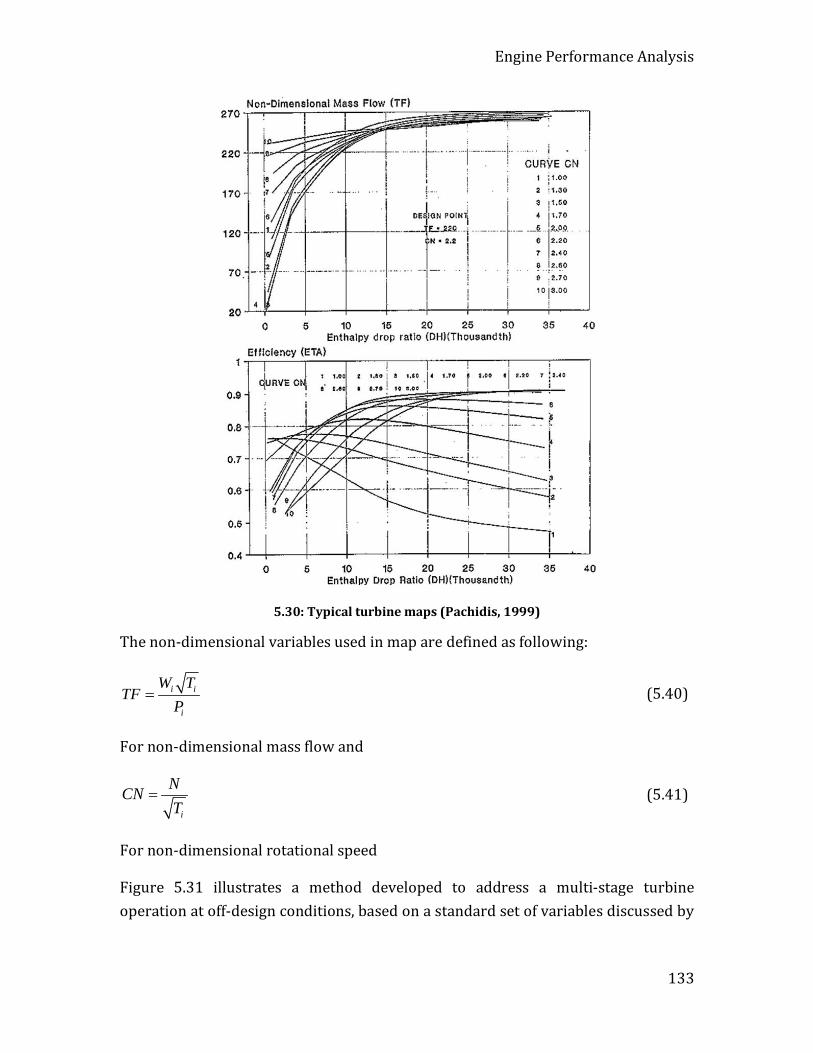
Engine Performance Analysis
133
5.30: Typical turbine maps (Pachidis, 1999)
The non-dimensional variables used in map are defined as following:
i i
i
W TTF
P= (5.40)
For non-dimensional mass flow and
i
NCNT
= (5.41)
For non-dimensional rotational speed
Figure 5.31 illustrates a method developed to address a multi-stage turbine operation at off-design conditions, based on a standard set of variables discussed by
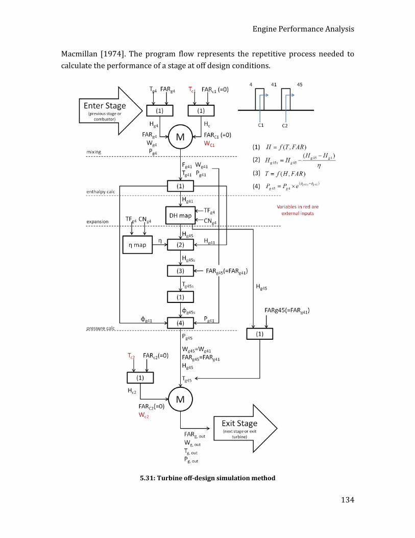
Engine Performance Analysis
134
Macmillan [1974]. The program flow represents the repetitive process needed to calculate the performance of a stage at off design conditions.
5.31: Turbine off-design simulation method
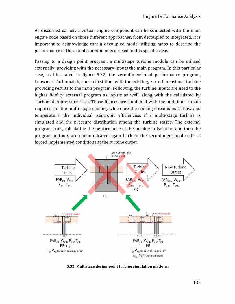
Engine Performance Analysis
135
As discussed earlier, a virtual engine component can be connected with the main engine code based on three different approaches, from decoupled to integrated. It is important to acknowledge that a decoupled mode utilising maps to describe the performance of the actual component is utilised in this specific case.
Passing to a design point program, a multistage turbine module can be utilised externally, providing with the necessary inputs the main program. In this particular case, as illustrated in figure 5.32, the zero-dimensional performance program, known as Turbomatch, runs a first time with the existing, zero-dimensional turbine providing results to the main program. Following, the turbine inputs are used to the higher fidelity external program as inputs as well, along with the calculated by Turbomatch pressure ratio. Those figures are combined with the additional inputs required for the multi-stage cooling, which are the cooling streams mass flow and temperature, the individual isentropic efficiencies, if a multi-stage turbine is simulated and the pressure distribution among the turbine stages. The external program runs, calculating the performance of the turbine in isolation and then the program outputs are communicated again back to the zero-dimensional code as forced implemented conditions at the turbine outlet.
5.32: Multistage design-point turbine simulation platform

Engine Performance Analysis
136
This way, the program is able to calculate the performance of the engine model, based on the results provided by a higher fidelity module, without having to fully integrate it to the main code. It is therefore, a semi-coupled approach.
5.8.3 Design Point Case Study A design point case study has been completed, based on the last semi-coupled approach. The study is referred to a design space investigation of an engine based at the Pratt & Whitney E3 [Gray, 1978], as discussed earlier. In this particular scenario, the performance of different engine cycles was assessed, first with a conventional simulation based on a zero-dimensional approach. Three different TET were examined, at 1613K, 1713K, which is the base case and 1813K. Thirteen different high pressure compressor pressure ratios were considered as well, from 4.8 to 28.8, with 12.8 being the base case, and the actual pressure ratio of the engine compressor at take-off conditions. At this exploration, the isentropic efficiency of the high pressure turbine was assumed to remain constant, as usually happens in similar investigations.
Following, the results from every one of these thirty nine simulations were input to the single-stage higher fidelity code, which calculated the performance of the turbine based on the method described earlier. Among the results was the thermodynamic efficiency as well, as defined in paragraph 5.4.2.
As the design space investigation was initially performed based on a constant isentropic efficiency assumption, a question may arise is why this happens. Isentropic efficiency describes the quality of the expansion process, but does not include the effects of cooling, as thermodynamic efficiency does. For this reason, an exploration of the design space based on a constant thermodynamic efficiency would make perfect sense, as the engine under investigation is heavily cooled and this is not reflected to the results or the conclusions of the case study.
The same process was therefore repeated. The cooled turbine external module was set to keep constant the thermodynamic efficiency of the base case (HPC PR=12.8, TET=1713K) and allow the isentropic efficiency to float, as a function of it. All other parameters remained constant: The turbine input vectors and the coolant mass flow and temperature. The isentropic efficiency fluctuation is illustrated in figure 5.33.

Engine Performance Analysis
137
5.33: Isentropic efficiency and power for different HPC pressure ratios and constant thermodynamic efficiency
It can be observed that for small pressure ratios a constant thermodynamic efficiency is translated into a high isentropic efficiency, which drops logarithmically until they intersect and continues having the same trend. An explanation for this behaviour is the fact that with increasing pressure ratio, the isobars deviate as well. As the calculation of thermodynamic efficiency is based on the actual work upon a number of ideal expansions from all the streams that flow through the turbine, a higher pressure ratio is translated into a higher deviation between the bounding lines of constant pressure at the enthalpy-entropy diagram. For small pressure ratios, the actual work is relatively closer to the ideal work of all the streams at the thermodynamic efficiency denominator. With increasing pressure ratios, the impact of the ideal expansions is getting more dominant, making the process less efficient, despite the increased work output.
Figure 5.34 illustrates the design space as discussed earlier, with the two different efficiencies kept constant.
20
25
30
35
40
45
50
55
60
65
0.86
0.87
0.88
0.89
0.9
0.91
0.92
0.93
0.94
0.95
4.8 8.8 12.8 16.8 20.8 24.8 28.8
Turb
ine
Pow
er [M
W]
Turb
ine
Effic
ienc
y [-]
HPC PR
nth nis Turbine Power
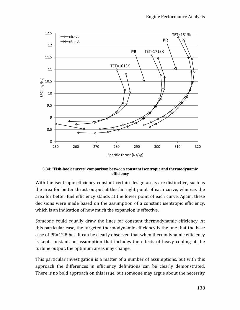
Engine Performance Analysis
138
5.34: “Fish-hook curves” comparison between constant isentropic and thermodynamic efficiency
With the isentropic efficiency constant certain design areas are distinctive, such as the area for better thrust output at the far right point of each curve, whereas the area for better fuel efficiency stands at the lower point of each curve. Again, these decisions were made based on the assumption of a constant isentropic efficiency, which is an indication of how much the expansion is effective.
Someone could equally draw the lines for constant thermodynamic efficiency. At this particular case, the targeted thermodynamic efficiency is the one that the base case of PR=12.8 has. It can be clearly observed that when thermodynamic efficiency is kept constant, an assumption that includes the effects of heavy cooling at the turbine output, the optimum areas may change.
This particular investigation is a matter of a number of assumptions, but with this approach the differences in efficiency definitions can be clearly demonstrated. There is no bold approach on this issue, but someone may argue about the necessity
8
8.5
9
9.5
10
10.5
11
11.5
12
12.5
250 260 270 280 290 300 310 320
SFC
[mg/
Ns]
Specific Thrust [Ns/kg]
nis=ct nth=ct
TET=1613K
TET=1713K
TET=1813K
PR
PR
Turbine Cooling Platform Discussion and Applications
139
of both efficiencies. It is certain that both describe a number of different properties. Therefore, someone exploring the design of a cycle should keep in mind that the effects of cooling are highly effective on every thermodynamic cycle and should be annexed when a decision must be taken. Moreover, as the temperature of coolant when rejoining the main cycle is an important parameter, the heat transfer analysis, as presented in chapter 3 is essential for the better determination of a cycle of choice.
5.9 Turbine Cooling Platform Discussion and Applications Chapters 4 and 5 presented a turbine simulation framework, which starts from a local heat transfer analysis level, expands to turbine performance on a larger scale, which is ultimately applicable to a gas turbine performance level. All this process could well be wrapped into a web-based performance simulation program, which can combine preliminary turbine design elements, along with life prediction elements and performance simulation, overall.
The need for such a workflow can be identified into the following three points:
First, the determination of turbine coolant temperature and mass flow is a significant figure for the overall turbine performance prediction. There are different ways to perform this analysis, but there always need to be a compromise between accuracy and complexity / usability.
Second, the coolant mass flow and temperature can be predicted based on empirical correlations, or based on physics enhanced by semi-empirical inputs. Either way, the method needs to be able to capture the influence of spatially variable boundary conditions, as the gas state changes significantly through an HPT.
Third, the influence of cooling at the overall gas turbine performance is substantial, and a main component of this influence is the needed mass flow and the resulted coolant temperature. A variation in these figures can be criterion for the approval or rejection of a certain design, which needs to be efficient, financially attractive and environment-friendly.
The simulation framework is most suitable for preliminary design of the cooling system, where the level of technology needs to be determined and evaluated in engine performance terms. It can work forward, starting from a certain blade design and desired cooling level, leading to engine performance, or backwards, starting

Turbine Cooling Platform Discussion and Applications
140
from a desired engine performance, which then is translated into a certain level of cooling technology for a certain blade design.
Either way, detailed gas flow data around the blade are a valuable input, but not a prerequisite. Having them, a designer can better predict the actual cooling demands, which are translated into a required coolant mass flow. Additionally, a detailed flow field indicates the actual blade points that need attention in cooling, along with a detailed and indicative blade temperature distribution for further analysis, such as creep life prediction.
The flow prediction can be made with flow analysis tools such as CFD, as performed in chapter 4, or even lighter solvers, such as MISES [Drela, 2008] [Andrew, 2009] or other Euler solvers. The possible inputs from this analysis are the gas temperature and heat transfer coefficient in the desired resolution (one- to three-dimensional). The latter is a crucial input, which is not always possible to obtain in details, since the setup of the blade wall boundary conditions can be a task that needs attention. Alternatively, experimental, empirical or even uniform heat transfer coefficient inputs may be used, keeping in mind the corresponding limitations each time. In any case, the tool is equally applicable in comparing results from different designs, providing an assessment among different designs.
A higher resolution turbine simulation (compared to zero-dimensional) requires a number of additional inputs. These inputs include an assumption for the work (or enthalpy, or pressure ratio) distribution among the stages, individual stage isentropic efficiencies and coolant mass flow rate and temperature for every stream. As long as the last are indicated by a knowledgeable prediction, the turbine analysis will be more complete, when such a requirement is set. This may well be the case of an engine preliminary design, as stated earlier.
In order this analysis to be translated into an engine-level simulation, additional inputs are required for all the other engine components as well. The detailed specifications for all of them may not be available, but again, this analysis can produce comparative results, which can be indicative on different trends at the engine parameters, or to provide an order of magnitude to the impact of a certain design decision. This analysis, could be much more easy to perform with a tool such the WebEngine, Which will be presented in chapter 6. In the WebEngine, engine templates are already developed with complete inputs, and the user will be able to change plug-in components, based on a standard interconnection interface. This will

Turbine Cooling Platform Discussion and Applications
141
be much more accessible as well from the web, where the demands from local resources will only be limited into the internet connectivity.
142
6 A Web-based Gas Turbine Performance Simulation Tool
6.1 Introduction Gas turbine simulation has always been a field of extensive research in the jet engine era. A large number of simulation codes have been released during the last decades, covering a wide range of applications, code structures and degrees of fidelity [NATO-RTO, 2002]. The WebEngine is a gas turbine simulation tool developed to fill a certain gap: Remote accessibility.
The computational power of modern computers has significantly grown over the years, followed by the development of much more advanced simulation codes and applications. More advanced cycles and complex engines configurations were introduced, while the code structure and component interchangeability were proved to be significant for some research applications. In addition, simulation methods as the ones presented in previous chapters are becoming increasingly popular, since they can be valuable engine design tools, in combination with overall cycle prediction programs.
In many cases, the need for local installation becomes an impediment for a wider popularity. An indicative application can be identified in academic institutes, where gas turbine performance lectures may be enriched with tutorial sessions of various performance case studies, but the performance program must be installed on every computer in the laboratory. Another example is student assignments, where there is

Introduction
143
the need for installation at the students’ personal computers. Part-time students, exchange students, short course delegates are also user categories that need remote access to performance simulation tools, since they usually work off-campus. In addition, gas turbine maintenance engineers need to access their simulation and diagnostics data on site. Local installation and the associated license issues can a matter of discussion in all of these user categories.
The WebEngine is a gas turbine performance simulation tool which is online accessible from any part of the world, with the only requirement being a web browser and an internet connection. The WebEngine is composed of two main parts: First, a gas turbine performance simulation solver, which is the core of the application and second, a dedicated web-based Graphical User Interface and client-server architecture configuration for remote access.
Turbomatch, which is the core solver of WebEngine, is a piece of performance simulation software, developed throughout the years by the former Department of Power and Propulsion at the School of Engineering of Cranfield University. The code has proved to be very stable and accurate and therefore it has contributed to a large number of student theses, research work and publications. Some indicative examples include Li [2004], Pachidis [2006a] and Giannakakis [2011]. Turbomatch is structured in a modular architecture, which enables interchangeable engine components and future developments. Moreover, the code is developed in a way that enables integration with other tools, such as higher fidelity components as the one-dimensional turbine presented in chapter 5, the cooling prediction module presented in chapter 4 and others, optimisers and flow solvers.
Passing to the WebEngine GUI and remote accessibility, the Client-Server architecture is considered to be a unique feature among the performance simulation programs. Currently, the WebEngine is hosted as a website in a server located at Cranfield University and open to end users through the World Wide Web. A virtual engine solver is allocated to every user, along with a group of preconfigured engines, accessible at anytime. The performance results are communicated back to the user through the website, and can be downloaded locally as well, on a data file format. It can be noted that apart from personal computers, any device browsing the web, such as mobile phones and tablets has access to the virtual environment.
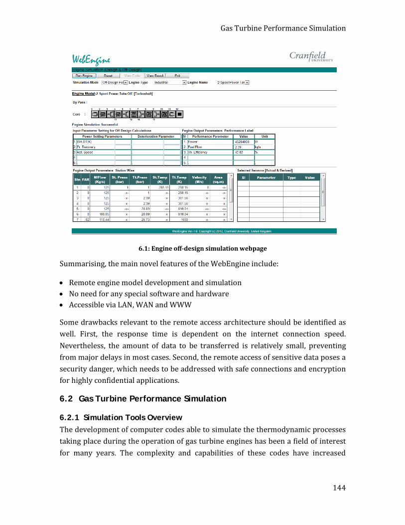
Gas Turbine Performance Simulation
144
6.1: Engine off-design simulation webpage
Summarising, the main novel features of the WebEngine include:
• Remote engine model development and simulation • No need for any special software and hardware • Accessible via LAN, WAN and WWW
Some drawbacks relevant to the remote access architecture should be identified as well. First, the response time is dependent on the internet connection speed. Nevertheless, the amount of data to be transferred is relatively small, preventing from major delays in most cases. Second, the remote access of sensitive data poses a security danger, which needs to be addressed with safe connections and encryption for highly confidential applications.
6.2 Gas Turbine Performance Simulation
6.2.1 Simulation Tools Overview The development of computer codes able to simulate the thermodynamic processes taking place during the operation of gas turbine engines has been a field of interest for many years. The complexity and capabilities of these codes have increased
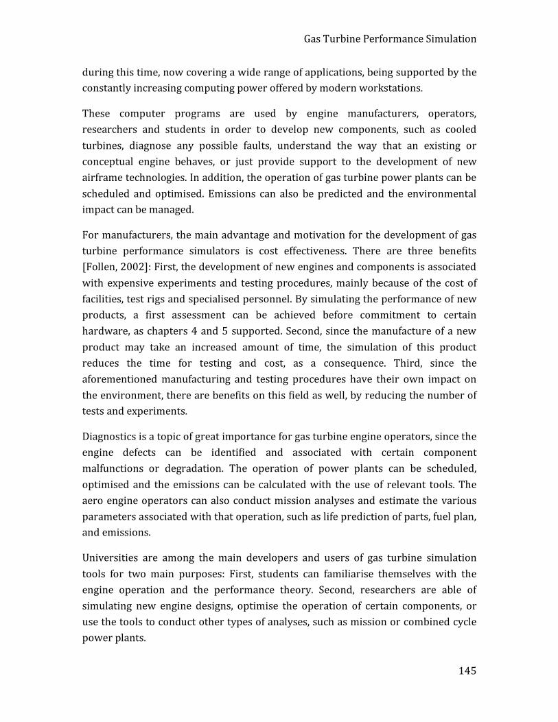
Gas Turbine Performance Simulation
145
during this time, now covering a wide range of applications, being supported by the constantly increasing computing power offered by modern workstations.
These computer programs are used by engine manufacturers, operators, researchers and students in order to develop new components, such as cooled turbines, diagnose any possible faults, understand the way that an existing or conceptual engine behaves, or just provide support to the development of new airframe technologies. In addition, the operation of gas turbine power plants can be scheduled and optimised. Emissions can also be predicted and the environmental impact can be managed.
For manufacturers, the main advantage and motivation for the development of gas turbine performance simulators is cost effectiveness. There are three benefits [Follen, 2002]: First, the development of new engines and components is associated with expensive experiments and testing procedures, mainly because of the cost of facilities, test rigs and specialised personnel. By simulating the performance of new products, a first assessment can be achieved before commitment to certain hardware, as chapters 4 and 5 supported. Second, since the manufacture of a new product may take an increased amount of time, the simulation of this product reduces the time for testing and cost, as a consequence. Third, since the aforementioned manufacturing and testing procedures have their own impact on the environment, there are benefits on this field as well, by reducing the number of tests and experiments.
Diagnostics is a topic of great importance for gas turbine engine operators, since the engine defects can be identified and associated with certain component malfunctions or degradation. The operation of power plants can be scheduled, optimised and the emissions can be calculated with the use of relevant tools. The aero engine operators can also conduct mission analyses and estimate the various parameters associated with that operation, such as life prediction of parts, fuel plan, and emissions.
Universities are among the main developers and users of gas turbine simulation tools for two main purposes: First, students can familiarise themselves with the engine operation and the performance theory. Second, researchers are able of simulating new engine designs, optimise the operation of certain components, or use the tools to conduct other types of analyses, such as mission or combined cycle power plants.

Gas Turbine Performance Simulation
146
6.2.2 Simulation Tools Classification There are a number of different ways to classify the commercial gas turbine simulation tools. First, the intended use may vary and aim on research, education or industrial use, such as life prediction, diagnostics or power plant planning and optimisation. Of course, some of these applications may overlap and some of the programs may be suitable for more than one intended use.
Historically, most codes have been developed as zero-dimensional, where the components are developed as ‘black-boxes’, without any physical dimensions simulated. In other words, the components were developed to transform a given input to a certain output. This is the case for the standard version of the WebEngine and its core solver, Turbomatch. The necessary correlations between the inputs and outputs of most components are dictated by component maps, ultimately providing the outlet conditions. This approach is sufficient for overall performance calculations, but it is not suitable when the internal component operation is of interest, as with the one-dimensional turbine of chapter 5.
On the other hand, the programs in most cases imitate the configuration of actual engines, providing results based on virtual component calculations, such as compressors, combustors and turbines. This does not necessarily means that all codes are modular in practice. Despite the fact that discrete components are used in most cases, there are codes providing interchangeable components, where an engine model can be assembled by serially stacking modules, or in other cases the structure is fixed and the user has no control on the engine layout in the first place.
As informatics technology evolved, increased simulation capabilities have been developed and higher fidelity components started being used. Such an approach may not be suitable just for overall cycle calculations, but it is very useful when the aim is the design of components, the performance of which can now be evaluated as part of the whole engine. Modern simulation codes may partly include higher fidelity components, or may be completely composed of higher resolution parts. This last approach makes the use of modular structure favourable.
Passing to a brief overview of the main commercial gas turbine performance simulation programs, GasTurb, GSP, NPSS and PROOSIS will be first examined, in comparison with the WebEngine
GasTurb [Kurzke, 2007] is under development since 1991, being a user-friendly fixed structure simulation program. It offers preset types of engines, with editable
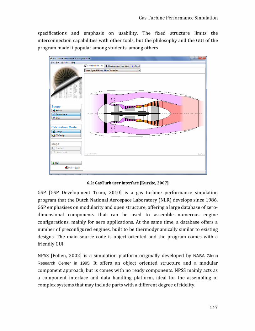
Gas Turbine Performance Simulation
147
specifications and emphasis on usability. The fixed structure limits the interconnection capabilities with other tools, but the philosophy and the GUI of the program made it popular among students, among others
6.2: GasTurb user interface [Kurzke, 2007]
GSP [GSP Development Team, 2010] is a gas turbine performance simulation program that the Dutch National Aerospace Laboratory (NLR) develops since 1986. GSP emphasises on modularity and open structure, offering a large database of zero-dimensional components that can be used to assemble numerous engine configurations, mainly for aero applications. At the same time, a database offers a number of preconfigured engines, built to be thermodynamically similar to existing designs. The main source code is object-oriented and the program comes with a friendly GUI.
NPSS [Follen, 2002] is a simulation platform originally developed by NASA Glenn
Research Center in 1995. It offers an object oriented structure and a modular component approach, but is comes with no ready components. NPSS mainly acts as a component interface and data handling platform, ideal for the assembling of complex systems that may include parts with a different degree of fidelity.
Gas Turbine Performance Simulation
148
PROOSIS [Alexiou, 2005] is a simulation environment for zero- or one-dimensional systems, designed for aerospace propulsion systems. It has been developed by a joint team of European researchers under the EU-funded VIVACE project. It is commercially available since 2008. It is modular and object-oriented as well. It offers a database of existing engine designs, but the user can assemble different engine designs, based on component libraries, or even develop new components, according to their individual requirements. The emphasis of PROOSIS is on aero engines as well.
6.3: PROOSIS user interface [Alexiou, 2006]
The Thermoflow GT PRO [www.thermoflow.com] platforms are specialised in Combined Cycle Gas Turbine power plants design, including all the involved components, apart from the gas turbine. The gas turbine in such simulations is just a component, interconnected with the rest of the plant, so there is no actual resolution of the engine. Therefore, the gas turbine is a black-box with a design point only operation.
GateCycle [www.ge-energy.com] is a Combine Cycle Gas Turbine and power plant simulator, developed by General Electric, offering a large database of industrial use
Gas Turbine Performance Simulation
149
gas turbines. It is able to simulate all the plant cycle as well, but it offers off-design point simulations as well, apart from design point.
There are a number of other programs as well, not necessarily dedicated to gas turbine performance simulation, but being able to simulate the processes taking place on industrial applications. Some examples are the Aspen Plus [http://www.aspentech.com/], which is a process modelling platform, offering a library of power plants processes, but in reality it is a more generic tool, and therefore is capable of design point only simulations. Other tools can be programmed as well in a way that simulates the operation of gas turbines as part of industrial complexes, such as MODELICA [https://www.modelica.org/] or TRNSYS [http://www.trnsys.com/], a piece of software dedicated to transient process simulation.
As a general observation, a modular structure vastly increases the program flexibility but still, there are degrees of modularity. NPSS provides users with complete flexibility to develop components and to make them interact based on any law they need. PROOSIS and GSP, provide the same freedom for module stacking, but the laws that associate the modules performance are predetermined. This is the case with the WebEngine as well, where existing or new components need to follow a certain interface to plug-in. GasTurb is even more restricted, as it does not offer any flexibility on component stacking, as the engine layouts are fixed and controlled by the source developer.
On the other hand, someone may argue that the higher the modularity and flexibility they are, the lower the user-friendliness it is. Indeed, on a program that offers numerous options of components and interconnection methods, an entry level user will need a large amount of time, in order to get familiarised with the environment and start producing meaningful results from simulations. At this category of users, a program such as GasTurb has an advantage. The WebEngine tries to address this issue, providing a hybrid approach, which combines a number of ready-to-use models with a component library for new engine designs.
The same issues apply to Combined Cycle Gas Turbine power plants simulation programs, where any dedicated applications are easier to setup and run, while more generic platforms may have advantages on flexibility and simulation of novel configurations. Inevitably, they may require a much higher level of experience in order someone start producing results.

WebEngine Overview
150
Finally, an open architecture facilitates the interconnection of a program with external tools, such as optimisers or other kinds of solvers, including the cooling prediction method earlier presented. But again this kind of use requires users of higher level of skills and requirements.
6.3 WebEngine Overview The motivation for the development of a remotely accessible tool comes from the fact that demand for part-time or distance-learning courses is constantly increasing during the last years, as a matter of professional mobility and further personal development. In addition, part-time or visiting students increasing in numbers, demanding access to educative tools from their place of residence, as visits to their place of study are not always possible frequently. The same applies to short course delegates, who need access to the material they learned, even after the time of the lectures. A possible solution on that would be the local installation of a program, which as well poses some issues relevant to licensing, access to certain datasets and updating.
6.4: Engine design webpage
The WebEngine was conceptualised in early 2009, and since then it is on a constant development, guided by a development plan, along with feedback gained by a
WebEngine Overview
151
number of users. After a number of revisions, the present version has the following features:
• Design point and off-design point performance simulation • Component degradation • Inventory of preconfigured engines, able to be reconfigured and modified • Design of new engine models in a modular way • Virtual sensor selection and data monitoring • Multiple point parametric analysis and plotting • Gas turbine power plant operation scheduling
The core solver of WebEngine is Turbomatch, a gas turbine performance simulation tool developed by the former Department of Power and Propulsion, Cranfield Univeristy. Turbomatch is capable of running standalone as well. The code has evolved through many successive development periods during the last four decades and its modular and open architecture of Turbomatch enables the interconnection with other, external tools, such as higher fidelity components, optimisers or other kinds of simulators, including cooling prediction tools.
The first version of Turbomatch was developed by MacMillan [1974] and a number of other developers contributed as well, such as van den Hout [1991], Sirinogou [1992], Ezkerra Fernandez [2003], Pachidis [2006b], Kyritsis [2006], Jannikovic [2010] and Giannakakis [2013]. Although major updates and additions followed the initial release, the basic code structure and philosophy remain the same until today. As with many other engineering applications, the code was written in FORTRAN, a programming language selected for all the versions until today. The code is capable of performing design point, off-design and transient simulations of any civil, military or industrial gas turbine configuration and includes a number of simulation capabilities, such as degraded component performance, different fuels, water injection and ingestion and variable compressor and turbine geometry. With the classic Turbomatch interface, the communication of the results is achieved with the use of input and output files. This approach can be advantageous for some user categories, as it is more flexible, but the effort required for the creation of an input file is an unnecessary or long task sometimes, which is a clear advantage of the WebEngine.
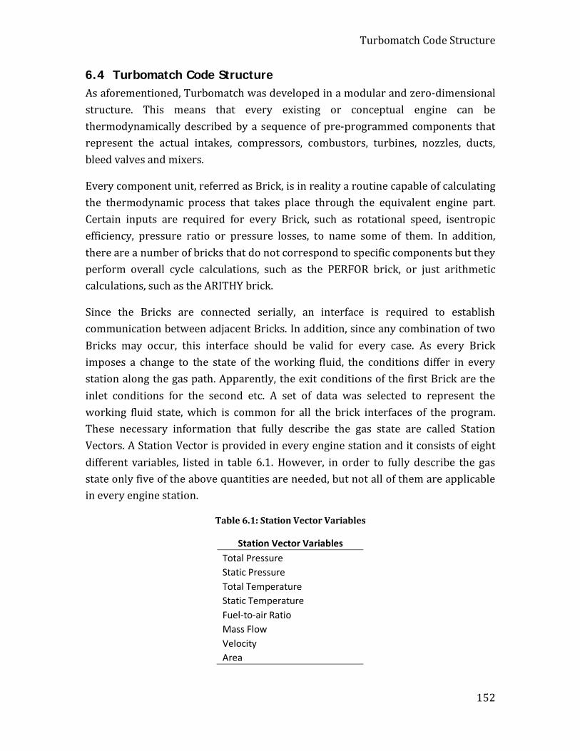
Turbomatch Code Structure
152
6.4 Turbomatch Code Structure As aforementioned, Turbomatch was developed in a modular and zero-dimensional structure. This means that every existing or conceptual engine can be thermodynamically described by a sequence of pre-programmed components that represent the actual intakes, compressors, combustors, turbines, nozzles, ducts, bleed valves and mixers.
Every component unit, referred as Brick, is in reality a routine capable of calculating the thermodynamic process that takes place through the equivalent engine part. Certain inputs are required for every Brick, such as rotational speed, isentropic efficiency, pressure ratio or pressure losses, to name some of them. In addition, there are a number of bricks that do not correspond to specific components but they perform overall cycle calculations, such as the PERFOR brick, or just arithmetic calculations, such as the ARITHY brick.
Since the Bricks are connected serially, an interface is required to establish communication between adjacent Bricks. In addition, since any combination of two Bricks may occur, this interface should be valid for every case. As every Brick imposes a change to the state of the working fluid, the conditions differ in every station along the gas path. Apparently, the exit conditions of the first Brick are the inlet conditions for the second etc. A set of data was selected to represent the working fluid state, which is common for all the brick interfaces of the program. These necessary information that fully describe the gas state are called Station Vectors. A Station Vector is provided in every engine station and it consists of eight different variables, listed in table 6.1. However, in order to fully describe the gas state only five of the above quantities are needed, but not all of them are applicable in every engine station.
Table 6.1: Station Vector Variables
Station Vector Variables Total Pressure Static Pressure Total Temperature Static Temperature Fuel-to-air Ratio Mass Flow Velocity Area
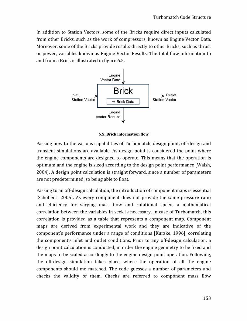
Turbomatch Code Structure
153
In addition to Station Vectors, some of the Bricks require direct inputs calculated from other Bricks, such as the work of compressors, known as Engine Vector Data. Moreover, some of the Bricks provide results directly to other Bricks, such as thrust or power, variables known as Engine Vector Results. The total flow information to and from a Brick is illustrated in figure 6.5.
6.5: Brick information flow
Passing now to the various capabilities of Turbomatch, design point, off-design and transient simulations are available. As design point is considered the point where the engine components are designed to operate. This means that the operation is optimum and the engine is sized according to the design point performance [Walsh, 2004]. A design point calculation is straight forward, since a number of parameters are not predetermined, so being able to float.
Passing to an off-design calculation, the introduction of component maps is essential [Schobeiri, 2005]. As every component does not provide the same pressure ratio and efficiency for varying mass flow and rotational speed, a mathematical correlation between the variables in seek is necessary. In case of Turbomatch, this correlation is provided as a table that represents a component map. Component maps are derived from experimental work and they are indicative of the component’s performance under a range of conditions [Kurzke, 1996], correlating the component’s inlet and outlet conditions. Prior to any off-design calculation, a design point calculation is conducted, in order the engine geometry to be fixed and the maps to be scaled accordingly to the engine design point operation. Following, the off-design simulation takes place, where the operation of all the engine components should me matched. The code guesses a number of parameters and checks the validity of them. Checks are referred to component mass flow

WebEngine Code Structure
154
compatibility, same shaft rotational speed, work compatibility and the power law for turbines driving generators.
Finally, Turbomatch uses a number of special input and output files in order to specify the cycle to be simulated and provide results. When an engine model is assembled at the WebEngine interface, an input file is automatically assembled for every engine and case The WebEngine returns a results file after the simulation, both of them according to a special Turbomatch format.
6.5 WebEngine Code Structure The WebEngine is developed in a way that takes advantage of Turbomatch capabilities, while at the same time offers an ergonomic graphical user interface and remote access. As schematically can be observed in figure 6.6, the front-end, developed as an ASP.NET application in C# language is the only part of the program that a user needs to know and handle. Everything is hosted on the server and accessed remotely via a page browser and through the World Wide Web.
6.6: WebEngine architecture
In the background, the engine console application coordinates the various parts of the program. First, the engine and user database are accessed through the console. Second, the engine performance simulator is executed as a dynamic-link library (DLL). This is actually a format of Turbomatch, individually available for every user logged in the website. The engine DLL is the unit that accesses and returns the input
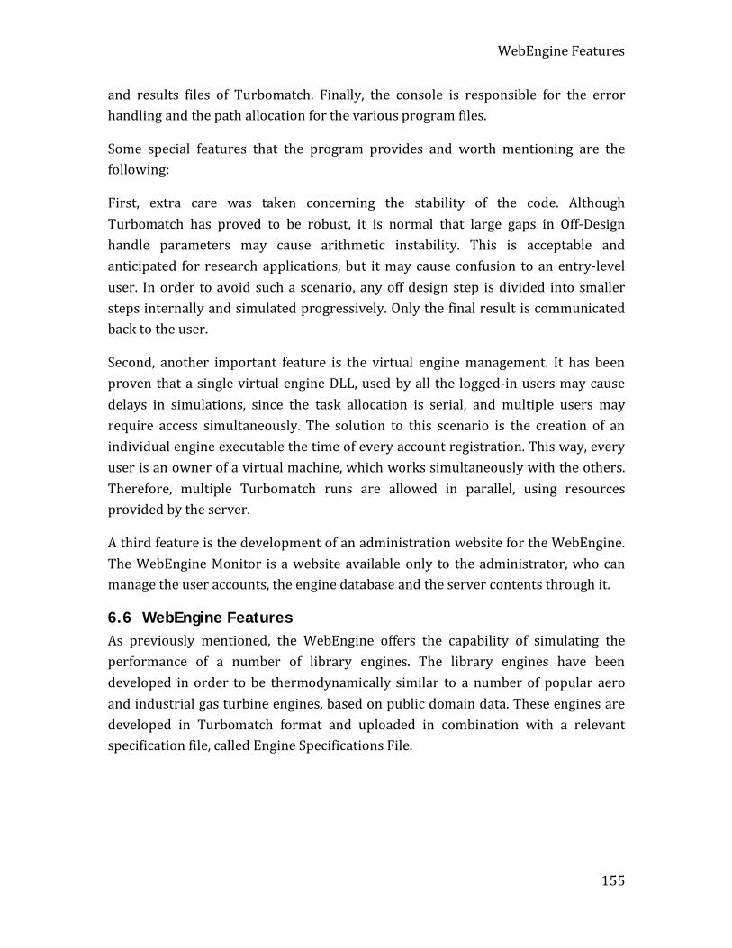
WebEngine Features
155
and results files of Turbomatch. Finally, the console is responsible for the error handling and the path allocation for the various program files.
Some special features that the program provides and worth mentioning are the following:
First, extra care was taken concerning the stability of the code. Although Turbomatch has proved to be robust, it is normal that large gaps in Off-Design handle parameters may cause arithmetic instability. This is acceptable and anticipated for research applications, but it may cause confusion to an entry-level user. In order to avoid such a scenario, any off design step is divided into smaller steps internally and simulated progressively. Only the final result is communicated back to the user.
Second, another important feature is the virtual engine management. It has been proven that a single virtual engine DLL, used by all the logged-in users may cause delays in simulations, since the task allocation is serial, and multiple users may require access simultaneously. The solution to this scenario is the creation of an individual engine executable the time of every account registration. This way, every user is an owner of a virtual machine, which works simultaneously with the others. Therefore, multiple Turbomatch runs are allowed in parallel, using resources provided by the server.
A third feature is the development of an administration website for the WebEngine. The WebEngine Monitor is a website available only to the administrator, who can manage the user accounts, the engine database and the server contents through it.
6.6 WebEngine Features As previously mentioned, the WebEngine offers the capability of simulating the performance of a number of library engines. The library engines have been developed in order to be thermodynamically similar to a number of popular aero and industrial gas turbine engines, based on public domain data. These engines are developed in Turbomatch format and uploaded in combination with a relevant specification file, called Engine Specifications File.
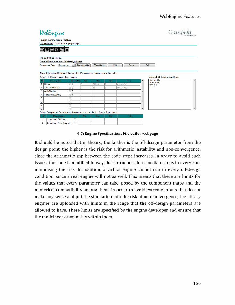
WebEngine Features
156
6.7: Engine Specifications File editor webpage
It should be noted that in theory, the farther is the off-design parameter from the design point, the higher is the risk for arithmetic instability and non-convergence, since the arithmetic gap between the code steps increases. In order to avoid such issues, the code is modified in way that introduces intermediate steps in every run, minimising the risk. In addition, a virtual engine cannot run in every off-design condition, since a real engine will not as well. This means that there are limits for the values that every parameter can take, posed by the component maps and the numerical compatibility among them. In order to avoid extreme inputs that do not make any sense and put the simulation into the risk of non-convergence, the library engines are uploaded with limits in the range that the off-design parameters are allowed to have. These limits are specified by the engine developer and ensure that the model works smoothly within them.
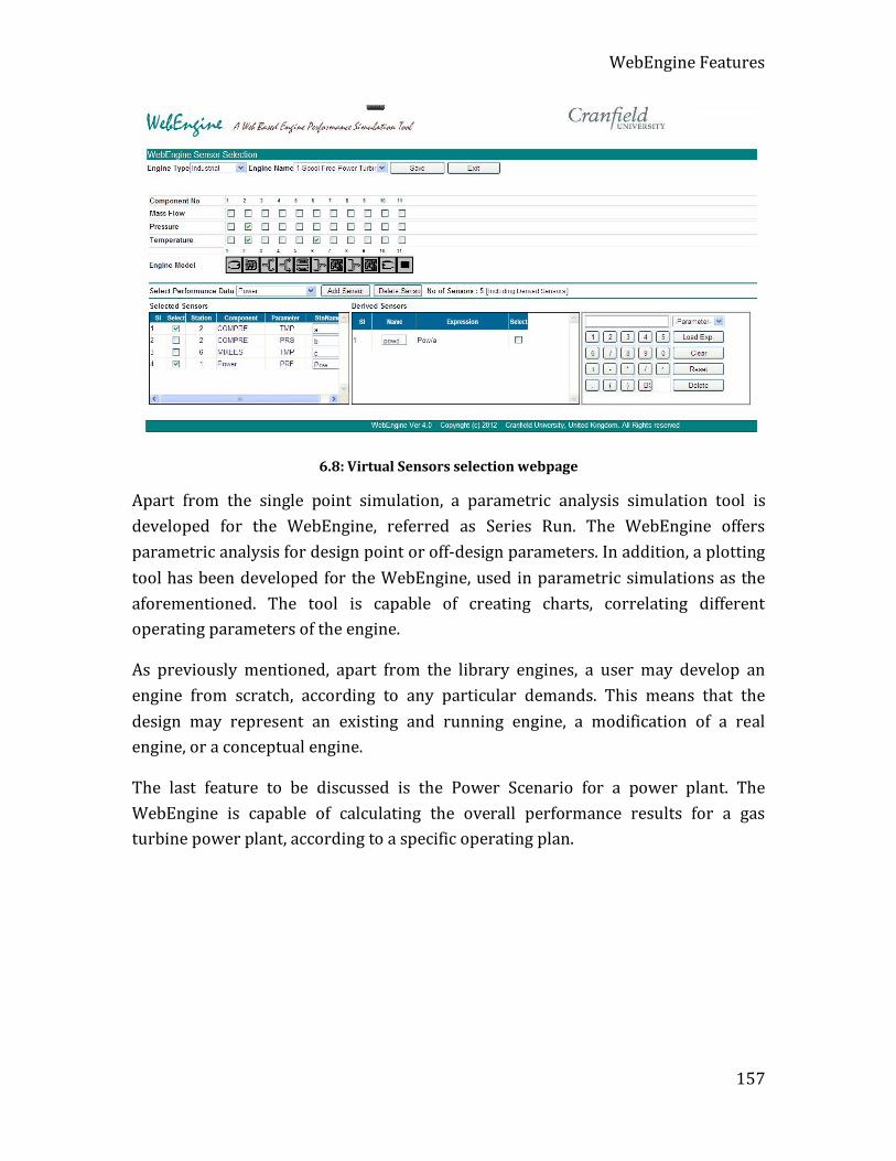
WebEngine Features
157
6.8: Virtual Sensors selection webpage
Apart from the single point simulation, a parametric analysis simulation tool is developed for the WebEngine, referred as Series Run. The WebEngine offers parametric analysis for design point or off-design parameters. In addition, a plotting tool has been developed for the WebEngine, used in parametric simulations as the aforementioned. The tool is capable of creating charts, correlating different operating parameters of the engine.
As previously mentioned, apart from the library engines, a user may develop an engine from scratch, according to any particular demands. This means that the design may represent an existing and running engine, a modification of a real engine, or a conceptual engine.
The last feature to be discussed is the Power Scenario for a power plant. The WebEngine is capable of calculating the overall performance results for a gas turbine power plant, according to a specific operating plan.
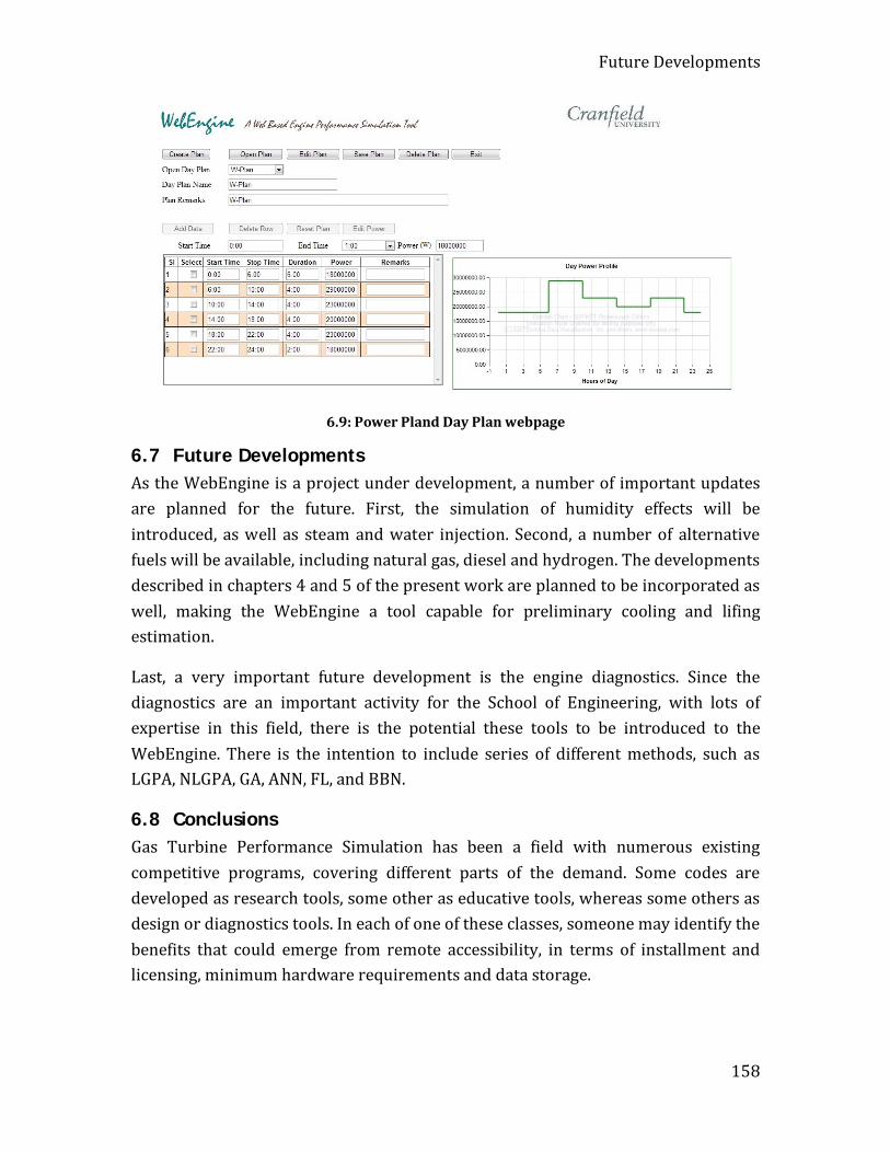
Future Developments
158
6.9: Power Pland Day Plan webpage
6.7 Future Developments As the WebEngine is a project under development, a number of important updates are planned for the future. First, the simulation of humidity effects will be introduced, as well as steam and water injection. Second, a number of alternative fuels will be available, including natural gas, diesel and hydrogen. The developments described in chapters 4 and 5 of the present work are planned to be incorporated as well, making the WebEngine a tool capable for preliminary cooling and lifing estimation.
Last, a very important future development is the engine diagnostics. Since the diagnostics are an important activity for the School of Engineering, with lots of expertise in this field, there is the potential these tools to be introduced to the WebEngine. There is the intention to include series of different methods, such as LGPA, NLGPA, GA, ANN, FL, and BBN.
6.8 Conclusions Gas Turbine Performance Simulation has been a field with numerous existing competitive programs, covering different parts of the demand. Some codes are developed as research tools, some other as educative tools, whereas some others as design or diagnostics tools. In each of one of these classes, someone may identify the benefits that could emerge from remote accessibility, in terms of installment and licensing, minimum hardware requirements and data storage.
Conclusions
159
The WebEngine have been developed in order to offer this feature, something that may be adopted by some of the other tools as well in the future. The fact that the WebEngine can be just updated in the server and this update is effective for all the users instantly makes all the planned future upgrades easy to implement. The future aspiration for the WebEngine is to be transformed into a platform that includes a library of higher fidelity components, including the one-dimensional turbine and the cooling prediction method presented earlier, making it suitable for the preliminary design of new engine components that can be immediately evaluated as part of the whole engine operation.
Currently, the tool is capable of design point and off-design simulations in single operating points, or in series. The WebEngine platform offers a database of different engine models, but provides also the flexibility the users to develop new engine models, according to their individual demands. Moreover, a power plant simulation tool is developed and offered as well.
Overall, the WebEngine is part of the platform presented in chapter 2, where the prediction of blade cooling requirements has a significant influence to the turbine operation and therefore the whole engine performance. Preliminary blade life estimation is possible as well, when combine with an external stress analysis, through this platform. This is an important aspect of modern gas turbine maintenance and cost planning, an important parameter even during the preliminary design phase. All this process can be significantly simplified when the special software used is user-friendly and offers all the aforementioned features.
Therefore, the final aspiration of this project is to make the WebEngine a hub, where all the simulation activities will be remotely accessible, for users with different backgrounds and requirements, wherever in the world they may be.
160
7 Conclusions and Future Work
7.1 Conclusions The thesis conclusions for every individual area of work are the following:
7.1.1 Turbine Blade Heat Transfer Method There are many different methods designed to predict the cooling requirements of turbines, based on different principals. Other methods focus on speed, thus numerous assumptions are required, while other methods focus on fidelity and therefore speed and simplicity are sacrificed. The simulation of a blade internal geometry is an indicative case where simplifications are required in the sake of speed, or because there is no alternative, if the actual geometry is not known, or not yet developed. Therefore, the selection of method is usually based on data and time availability.
The method presented in chapter 4 was developed in a way that captures the effects of gas flow through a turbine, but requires a limited amount of inputs, sufficient to predict the blade and coolant temperatures at all locations. The performed case studies provided the following conclusions:
The level of technology is represented by the averaged internal heat transfer coefficient of a single cooling channel. This last configuration is not indicative of modern cooling designs, but it was necessary to keep the method suitable for preliminary cooling calculations. In many cases, a person conducting cooling analysis has neither access to geometry data, nor to experimental data and needs a
Conclusions
161
starting point. In other cases, the blade design is not finalised. Therefore, the operator needs inputs for the cooling system design that this analysis can provide. In any case, validation showed that results can be close to reality with a careful parameter selection. The results can be translated into internal cooling configurations through the Z parameter [Horlock, 1973] and a number of other empirical correlations [Torbidoni, 2004a].
A parabolic gas temperature span distribution, which is typical for combustion outlet patterns, results on a blade temperature distribution with the maximum temperature between the mean line and blade tip. The exact location of this point for a given geometry is determined by the maximum parabola temperature deviation, the rate of convective heat transfer and the blade conductivity.
The modelling of conductivity is an addition that the present method introduced to the original, analytical and semi-empirical ones [Ainley, 1957] [Horlock, 1973] [Holland, 1980] [Consonni, 1992] [Horlock, 2006]. This development increased the complexity of calculations, but it can be justified by the results. As conduction tends to moderate temperatures at local peaks and to transfer heat to cooler areas, the topology of blade temperature can change to a high extent. The temperature of coolant is less sensitive at this change, but still there is an impact, as the rate of convective heat transfer is affected by the local temperature deviation between the blade wall and the coolant.
The introduction of a second modelling dimension was necessary for capturing the Mach and expansion effects of the gas flow. This development increased the amount of inputs required, along with a further addition in solving complexity. This is inevitable for such an analysis, as the details of the gas flow field contribute significantly to cooling prediction. This update was again developed for preliminary analysis requirements, utilising a simplified internal geometry as well. Someone could well use high-fidelity conjugate modelling to investigate the fluid-blade interaction, but this analysis is much more complex to set up. The method is able to provide temperature results for a thin-walled blade (which implies a single temperature value at the blade thickness direction) and conduction modelling. It is suitable for both stators and rotors, as the only difference is in boundary conditions.
The method results highlight the need to include the effects of gas acceleration and expansion to cooling calculations. The turbine entry temperature, when used for cooling calculations, is not indicative of the overall problem, including the case
Conclusions
162
where combustor cooling patterns are accounted. The reason is that gas acceleration through stators has a drastic effect on gas static temperatures that tends to drop and thus reduce the resulted local blade and coolant temperatures. But even when these effects are included as averaged values of a gas temperature field, again the fluctuations in blade temperatures are not captured, resulting to uniform blade temperatures, where life prediction is non-realistic.
Passing to rotors, the Mach number effects on local gas temperatures are combined with a total temperature drop due to expansion. This makes the need for detailed gas flow inputs more crucial. Indeed, again the use of rotor inlet total temperature for rotor cooling calculations results to overprediction of cooling requirements. This behaviour further justifies the need for chord modelling.
The modelling of conductivity is included as well to the two-dimensional model, as it can greatly affect a prediction. Conductivity modelling in chord direction tends to moderate any blade temperature peaks and valleys, affecting the local gradients, stresses due to non-uniform material expansion and ultimately, predicted life. When conduction is not accounted, the effect of gas inputs to every blade element are directly translated into a corresponding blade and coolant temperature, without being affected by any neighbouring element values, or by the slope of local temperatures.
A three-dimension model was further developed for the method of chapter 4. Here, the analysis is not based on discrete elements, but on a mean Biot number analysis, as executed by Horlock [2006]. The blade obtains a finite thickness, across which a temperature gradient is calculated. An important update includes the introduction of thermal barrier coatings modelling, based on the same principles. A limitation here is that, since there are no discrete thickness elements, the thermal diffusion at the chord direction is the same for the two material layers, a behaviour not realistic. The introduction of TBC though, results on lower calculated metal temperatures, which consecutively results on higher predicted blade creep life and lower coolant temperatures.
Film cooling is modelled as well based on film cooling effectiveness. The method modifies the gas temperature input, by mixing at every span location the corresponding gas and coolant and repeating the process until a converged coolant temperature is established. The method provides realistic trends in results, but is limited by the point where eventually the film and blade temperatures cross, where
Conclusions
163
a steep temperature gradient is present. The same limitation applies sometimes for high values of conductivity, where the resulted diffused blade temperature crosses the local gas temperature.
A significant limiting factor is the availability of detailed gas temperature and heat transfer coefficient data, or the need for numerical analysis to obtain these data. Gas turbine performance results are usually provided averaged, in various stations along the engine. The option of averaged data in any of the two input dimensions is available as well, resulting in useable data in the case of gas turbine performance, but not for blade temperature prediction.
The calculated coolant temperature and mass flow can be utilised by the multistage cooled turbine performance prediction method of chapter 5:
7.1.2 Multistage Cooled Turbine Method Coolant mass flow rate and outlet temperature are figures of significant importance for the determination of the actual turbine performance. This is due to the influence in gas mass flow and enthalpy, which is significant for modern, heavily cooled turbines. Turbine performance simulation can be performed with different degrees of fidelity. An axial resolution is important for correct allocation of the various cooling streams of multistage turbines and more realistic calculated work and temperatures. In addition, the calculation of thermodynamic efficiency is possible when individual cooling streams are accounted. The thermodynamic efficiency includes the ideal expansion of individual cooling streams, in order to provide a more extensive figure that accounts the actual turbine operation, including the contribution of cooling.
For a physically single-stage HPT, coolant used for stator cooling is contributing to the work produced, in contrast with coolant used for rotor and disc cooling. Thus, for a certain amount of coolant bled from the engine compressor, part of coolant contributes to work, expanding through the rotor and another part does not. In any case, despite the fact that gas enthalpy drops when mixing with the lower-temperature coolant, the additional mass dominates and the net effect is a turbine work increase, compared with the same turbine with no cooling involved.
The thermodynamic efficiency, which is affected by the amount of coolant contributing to work production, is constantly increasing with a higher amount of cooling air directed to stator. There is a certain proportion of cooling air distributed between the stator and rotor that equalises the thermodynamic and isentropic
Conclusions
164
efficiencies. This point remains the same for cooling streams of the same temperature, independently of the total amount of air available for cooling.
As coolant heats up along the blade, its enthalpy increases as well and producing a higher amount of turbine work through the rotor. In contrast, a higher coolant temperature implies a lower thermodynamic efficiency, as the work potential of the individual cooling streams increases as well, at a higher rate than the actual work produced. Consequently, a higher cooling efficiency at the blade implies a lower thermodynamic efficiency at the turbine.
The bookkeeping system of different parts may differ on the way that efficiency is calculated. Some cooling streams may be included or not for the definition of an ideal expansion, or they can be mixed or not before the expansion. Therefore, a same reference point must exist when results are discussed and exchanged.
When comparing a single-stage equivalent turbine model with a two-stage model of a physically two-stage HPT, results in power may differ to a certain extent. Extra attention is needed at the definition of the individual stage isentropic efficiencies, as they do not match with the isentropic efficiency of a single expansion, due to deviation of the isobars at the H-S diagram.
The predicted power and thermodynamic efficiency between the two models differ as well, since the allocation of cooling streams on different stages affects the amount and temperature of gas at the inlet of each rotor, compared with a single-rotor expansion. Additionally, the gas temperature along the different stations of a multistage turbine can only be predicted with a multistage model, as the stations of the SSE model do not correspond to the real turbine stations.
The deviation of turbine work between the two models increases with an increasing total amount of cooling air, as the two methods match when no cooling air is involved. In that case, the two individual expansions of the MCT match the single epansion of the SSE. The same applies with the thermodynamic efficiency of the two models, which match the isentropic for no cooling. For an increasing total amount of cooling air, equally distributed between the blade rows, thermodynamic efficiencies drop. This is a result of the wasted air at the end of the turbine.
Again, an increasing coolant temperature increases the work predicted by both the MCT and SSE models, while a higher coolant temperature results on a lower
Conclusions
165
thermodynamic efficiency for the same reason as previously: the higher work potential of the individual cooling streams that remains unexploited.
The pressure ratio split assumption between the stages provides a higher work output for the first stage, even with a 50%-50% distribution. This is due to the higher pressure boundaries in between the first stage operates. The difference in produced work apparently increases with more unequal PR distribution. But even the total amount of work produced decreases as well, and this is due to the assumed constant stage isentropic efficiencies along this parametric analysis. A constant polytropic efficiency would be preferable in such cases.
On an engine design level, an increasing HPC PR analysis was performed, as a study for different designs evaluation. The thermodynamic efficiency of the engine’s HPT was kept constant with increasing PR and the fluctuation in isentropic efficiency was captured. By going to higher pressure rations, the constant pressure lines at the H-S diagram deviate more, increasing the contribution of the individual ideal cooling flows expansions to the definition of the thermodynamic efficiency. The same effect is encountered at the design space of the SFC-Specific Thrust diagram of this new engine design. The constant TET lines differ, according to which efficiency is kept constant. Therefore, a common efficiency definition is important between collaborating parts, as the optimum engine design (for minimum SFC, for instance) can differ when different efficiency definitions are involved.
7.1.3 Web-Based Gas Turbine Performance Simulation It should be acknowledged that different gas turbine performance simulation programs are addressing to different audiences. Some codes are more research-oriented, while others are operators-oriented and some other education-oriented. Benefits in remote accessibility can be identified in all three categories: No local installation is needed, license and updates management are more direct and centrally controlled, and the requirements in hardware and local data storage are minimum. Moreover, data accessibility from different locations is an important advantage.
In chapter 6, a web-based gas turbine performance simulation tool was presented. The WebEngine was developed offering remote accessibility on design and off-design point simulation, in single operating points, or in series. Moreover, the modular structure and the engine library make the tool ideal for both beginners and advanced users, as ready models can be used by the former, while new, or even

Future Work
166
conceptual engine designs can be developed by the latter. A gas turbine power plant planning interface was developed as well.
The WebEngine is part of the platform presented in chapter 2, where the prediction of blade cooling requirements contributes to the prediction of turbine and continuing the whole engine performance.
7.2 Future Work A number of recommendations can be made for the future development of this work.
First, as the turbine blade heat transfer prediction method imposes a heat flux direction from the gas to the blade, the inverse process is impossible. This behaviour results in some cases to a crossing between the gas and predicted blade temperature, due to conductivity effects. This can be addressed with modelling the processes to take place in both directions.
Second, the method was developed to address steady state problems. This can be identified in the right-hand side of equations 4.6, 4.7, 4.27, 4.28, 4.36 and 4.38, which is equal to zero. Transient heat transfer modelling is possible, with introducing a heat surplus or deficit for small time intervals. This could model the acceleration or deceleration of the HPT.
The method was developed with a simplified internal geometry, for the sake of simplicity and applicability in preliminary design. Someone, following the same modelling principles, he could develop more detailed models, applicable at certain, fixed geometries. Moreover, the same modelling approach is applicable to other gas turbine heat transfer problems in different scales, such as impingement cooling or local heat transfer around film cooling orifices.
Another update could be the development of a blade cooling model with discrete elements at the thickness direction. This way, the heat diffusion at different layers could be accounted and simulated. More complex internal geometries could be developed as well, as with different layers the built of different internal geometries is favourable.
Going to the multistage turbine cooling simulation method, a mixing loss model could be introduced as well, to account the losses of coolant/gas mixing process. There are numerous relevant models developed based on empirical data and

Future Work
167
reviewed by Wei [2000], so the selection of a suitable one would be beneficial for the results.
The off-design simulation of multistage cooled turbines could be introduced, as presented schematically in figure 5.31. The added complexity of such an venture has to do with the use of individual stage maps, the relation of the individual isentropic efficiencies with the total turbine isentropic efficiency and the component coupling with the main code, as it needs to be fully integrated.
All these updates could be fully integrated to WebEngine, which can offer in the future a turbine cooling platform that starts from the very fundamentals of heat transfer and translate them into design, off-design point and transient gas turbine performance simulation.
168
References A
Ainley, D.G., 1957, “Internal Air Cooling for Turbine Blades: A General Design Survey,” Reports and Memo No. 3013, Aeronautical Research Council, Ministry of Supplies, London, UK, 1957.
Alexiou, A., and Mathioudakis, K., 2005. "Development of Gas Turbine Performance Models Using a Generic Simulation Tool," Proceedings of ASME Turbo Expo 2005, Reno, NV, USA, June 2005, Paper No. GT2005-68678, pp. 185-194.
Alexiou, A., and Mathioudakis, K., 2006. "Gas Turbine Engine Performance Model Applications Using an Object-Oriented Simulation Tool," Proceedings of ASME Turbo Expo 2006, Barcelona, Spain, June 2006, Paper No. GT2006-90339, pp. 109-116.
Alexiou, A., Baalbergen, E.H., Kogenhop, O., Mathioudakis, K., and Arendsen, P., 2007, “Advanced Capabilities for Gas Turbine Engine Performance Simulations,” Proceedings of ASME Turbo Expo 2007, Montreal, Canada, June 2007, Paper No. GT2007-27086, pp. 19-28.
Andrew, P.L., and Kahveci, H.S., 2009, "Validation of MISES Two-Dimensional Boundary Layer Code for High-Pressure Turbine Aerodynamic Design," Journal of Turbomachinery, Vol. 131, No. 3, 031013-1.
Aretakis, N., Roumeliotis, I., and Mathioudakis, K., 2011, "Performance Model “Zooming” for In-Depth Component Fault Diagnosis", Journal of Engineering for Gas Turbines and Power, Vol. 133, No. 3, 031602-1.
Aspen Plus, November 2013, [Online], URL: http://www.aspentech.com/products/aspen-plus.aspx, Cited November 2013
B
Ballal, D.R., and Zelina, J., 2004, “Progress in Aero Engine Technology (1939—2003),” Journal of Aircraft, Vol. 41, No. 1, pp. 43-50.
Bergeles, G., Gosman A.D., and Launder, B.E., 1978, “The Turbulent Jet in a Cross Stream at Low Injection Rates: A Three-Dimensional Numerical Treatment,” Numerical Heat Transfer, Vol. 1, No. 2, pp. 217–242.
169
Bindon, J.P., 1989, “The Measurement and Formation of Tip Clearance Loss,” Journal of Turbomachinery, Vol. 111, No. 3, pp. 257-263.
Birch N.T., 2000, “2020 Vision: The prospects for Large Civil Aircraft Propulsion,” The Aeronautical Journal, Vol. 104, No. 1038, pp. 347-352.
C
CFX-Pre User's Guide, January 2014, [online], URL: http://ccpbscm-1.central.cranfield.ac.uk/ansys/v140, Cited January 2014
Cheng, A.H.-D., and Cheng, D.T., 2005, “Heritage and Early History of the Boundary Element Method,” Engineering Analysis with Boundary Elements, Vol. 29, No. 3, pp. 268-302.
Ciepluch, C.C., Davis, D.Y., and Gray, D.E., 1987, "Results of NASA's Energy Efficient Engine Program," Journal of Propulsion, Vol. 3, No. 6, pp. 560-568.
Collin, J., 2004, “Impact of Aerothermal Modeling on the Estimation of Turbine Blade Life,” S.M. Thesis, Massachusetts Institute of Technology, Cambridge, MA, USA.
Consonni, S., 1992, “Performance Prediction of Gas/Steam Cycles for Power Generation,” PhD Thesis, Princeton University, Princeton, NJ, USA, PU/CEES Report No. 269.
D
Davis, D.Y., and Stearns, E.M., 1985, “Energy Efficient Engine – Flight Propulsion System Final Design and Analysis,” NASA-Lewis Research Center, Cleveland, OH, USA, NASA CR-168219.
de Wolf, W.B., Woldendorp, S., and Tinga, T., 2001, “Analysis of Combined Convective and Film Cooling on an Existing Turbine Blade,” National Aerospace Laboratory NLR, Amsterdam, The Netherlands, NLR-TP-2001-148.
Denton, J.D., 1993, “The 1993 IGTI Scholar Lecture: Loss Mechanisms in Turbomachines,” Journal of Turbomachinery, Vol. 115, No. 4, pp. 621–656.
Denton, J.D., and Dawes, W.N., 1998, "Computational Fluid Dynamics for Turbomachinery Design," Journal of Mechanical Engineering Science, Vol. 213, No. 2, pp. 107-124.
170
Dixon, S.L., 2005, Fluid Mechanics and Thermodynamics of Turbomachinery, Fifth Edition, Butterworth-Heinemann, Oxford, UK.
DLR (German Aerospace Center), 2013, Direct Numerical Simulations and Large Eddy Simulations – Theory, DLR, Göttingen, Germany.
Drela, M., and Youngren, H., 2008, A User’s Guide to MISES 2.63, Massachusetts Institute of Technology, Cambridge, MA, USA.
Duchaine, F., Corpron, A., Pons, L., Moureau, V., Nicoud, F., and Poinsot, T., 2009, "Development and assessment of a coupled strategy for conjugate heat transfer with Large Eddy Simulation: Application to a cooled turbine blade," International Journal of Heat and Fluid Flow, Vol. 30, No. 6, pp. 1129-1141.
Dunham, J., and Came, P.M., 1970, “Improvements to the Ainley-Mathieson Method of Turbine Performance Prediction,” Journal of Engineering for Gas Turbines and Power, Vol. 92, No. 3, pp. 252–256.
E
El-Masri, M.A., 1987, “Exergy Analysis of Combined Cycles: Part I - Air-Cooled Brayton-Cycle Gas Turbines,” Journal of Engineering for Gas Turbines and Power, Vol. 109, No. 2, pp. 228-236.
European Space Agency, April 2014, [online], URL: http://www.spaceflight.esa.int/impress/text/education/Heat%20Transfer/Conduction%2001.html, Cited April 2014
Ezkerra Fernandez, A., 2003, “Genetic Algorithms Based Combined Cycle Degradation Analysis and Turbomatch Design Point File Adaptation,” MSc Thesis, Cranfield University, Bedford, UK.
F
Follen, G., and auBuchon, M., 2000, “Numerical Zooming Between a NPSS Engine System Simulation and a One-Dimensional High Compressor Analysis Code,” NASA- Glenn Research Center, Cleveland, OH, USA, NASA TM-2000–209913.
171
Follen, G., 2002, “An Object Oriented Extensible Architecture for Affordable Aerospace Propulsion Systems” Proceedings of NATO-RTO AVT Symposium on “Reduction of Military Vehicle Acquisition Time and Cost through Advanced Modelling and Virtual Simulation,” Paris, France, April 2002, Paper No. RTO-MP-089.
G
Garg, V.K., Abhari, R.S, 1997, "Comparison of Predicted and Experimental Nusselt Number for a Film-Cooled Rotating Blade,” International Journal of Heat and Fluid Flow, Vol. 18, No. 5, pp. 452-460.
Garg, V.K., 1999, “Heat Transfer on a Film-Cooled Rotating Blade Using Different Turbulence Models,” International Journal of Heat and Mass Transfer, Vol. 42, No. 5, pp. 789-802.
GateCycle, April 2014, [online], URL: http://site.ge-energy.com/prod_serv/products/oc/ja/opt_diagsw/gatecycle.htm, Cited April 2014
Gauntner, J.W., 1994 "Turbine Cooling Flow and the Resulting Decrease in Turbine Efficiency," NASA-Lewis Research Center, Cleveland, OH, USA, NASA LEW-13999.
Giannakakis, P., Laskaridis, P. and Pilidis, P., 2011, "Effects of Offtakes for Aircraft Secondary-Power Systems on Jet Engine Efficiency," Journal of Propulsion and Power, Vol. 27, No. 5, pp. 1024-1031.
Giannakakis, P., 2013, “Design space exploration and performance modelling of advanced turbofan and open-rotor engines,” EngD Thesis, Cranfield University, Bedford, UK.
Goldstein, R. J., 1971, "Film Cooling," Advances in Heat Transfer, Vol. 7, pp. 321- 379.
Goldstein, R.J., and Jin, P., 2001, “Film Cooling Downstream of a Row of Discrete Holes With Compound Angle,” Journal of Turbomachinery, Vol. 123, No. 2, pp. 222-230.
Gray, D.E., et al., 1978, “Energy Efficient Engine - Preliminary Design and Integration Studies,” NASA-Lewis Research Center, Cleveland, OH, USA, NASA CR-135396.
Green, J.E., 2003, “Civil Aviation and the Environmental Challenge,” The Aeronautical Journal, Vol. 107, No. 1072, pp. 281-299.
172
GSP Development Team, 2010, GSP 11 User Manual, National Aerospace Laboratory NLR, Amsterdam, The Netherlands.
H
Hall, E.J., 2000, “Modular Multi-Fidelity Simulation Methodology for Multiple Spool Turbofan Engines,” Proceedings of the NASA High Performance Computing and Communications Computational Aerosciences Workshop, NASA-Ames Research Center, Mountain View, CA, USA.
Halls, G.A., 1967, "Air Cooling of Turbine Blades and Vanes," Aircraft Engineering and Aerospace Technology, Vol. 39, No. 8, pp. 4-14.
Han, J. C., Park, J. S., and Ibrahim, M. Y., 1986, “Measurement of Heat Transfer and Pressure Drop in Rectangular Channels with Turbulence Promoters,” NASA-Lewis Research Center, Cleveland, OH, USA, AVSCOM Technical Report 86-C-25.
Henze, M., Bogdanic, L., Muehlbaue, K., and Schnieder, M., 2013, "Effect of the Biot Number on Metal Temperature of Thermal-Barrier-Coated Turbine Parts - Real Engine Measurements," Journal of Turbomachinery, Vol. 135, No. 3, 031029.
Hodge, R.I., 1960a, “A Turbine Nozzle Cascade for Cooling Studies - Part I: The Measurement of Mean NusseIt Numbers at the Blade Surface,” Aeronautical Research Council, London, UK, C.P. No. 493.
Hodge, R.I., 1960b, “A Turbine Nozzle Cascade for Cooling Studies - Part II: Comparison between Measured and Predicted Mean Nusselt Numbers at the Blade Surface,” Aeronautical Research Council, London, UK, C.P. No. 493.
Holland, M.J., and Thake, T.F., 1980, “Rotor Blade Cooling in High Pressure Turbines,” Journal of Aircraft, Vol. 17, No. 6, pp. 412-418.
Horlock, J.H., 1973, Axial Flow Turbines: Fluid Mechanics and Thermodynamics, Krieger Pub Co, Huntington, NY, USA.
Horlock, J.H., Watson, D.T., and Jones, T.V., 2001a, “Limitations on Gas Turbine Performance Imposed by Large Turbine Cooling Flows,” Journal of Engineering for Gas Turbines and Power, Vol. 123, No. 3, pp. 487–494.
Horlock, J.H., 2001b "The Basic Thermodynamics of Turbine Cooling," Journal of Turbomachinery, Vol. 123, No. 3, pp. 583-592.
173
Horlock, J.H., and Torbidoni, L., 2006, “Turbine Blade Cooling: The Blade Temperature Distribution,” Journal of Power and Energy, Vol. 220, No. 4, pp. 343-353.
Howell, J.R., Siegel, R., and Pinar Menguc, M., 2002, Thermal Radiation Heat Transfer, Fifth Edition, CRC Press, Boca Raton, FL, USA.
Humble, L.V., Lowdermilk, W.H., and Desmond, L.G., 1951, "Measurements of Average Heat-Transfer and Friction Coefficients for Subsonic Flow of Air in Smooth Tubes at High Surface and Fluid Temperatures," NACA Report 1020.
J
Janikovič, J., 2007, The Turbomatch Scheme User Manual, Cranfield University, Bedford, UK.
Janikovič, 2010, “Gas Turbine Transient Performance Modeling for Engine Flight Path Cycle Analysis,” PhD Thesis, Cranfield University, Bedford, UK.
K
Kegalj, M., Winter, N., Schiffer, H.-P., Pyliouras, S., and Taege, J., 2007, “Through Flow Modelling of a Modern Turbine Stator Cooling System,” Proceedings of the 8th International Symposium on Experimental and Computational Aerothermodynamics of Internal Flows, Lyon, France, July 2007, Paper No. ISAIF8-0052.
Koff, B.L., 2004, “Gas Turbine Technology Evolution: A Designer's Perspective,” Journal of Propulsion and Power, Vol. 20, No. 4, pp. 577-595.
Kong, C., Kho, S., and Ki, J., 2006, "Component Map Generation of a Gas Turbine Using Genetic Algorithms," Journal of Engineering for Gas Turbines and Power, Vol. 128, No. 1, pp. 92-96.
Kool, G.A., 1996 "Current and Future Materials in Advanced Gas Turbine Engines," Journal of Thermal Spray Technology, Vol. 5, No. 1, pp. 31-34.
Kurzke, J., 1996, "How to Get Component Maps for Aircraft Gas Turbine Performance Calculations”, Proceedings of ASME Turbo Expo 1996, Birmingham, UK, June 1996, Paper No. 96-GT-164.
174
Kurzke, J., 2002, “Performance Modeling Methodology: Efficiency Definitions for Cooled Single and Multistage Turbines”, Proceedings of ASME Turbo Expo 2002, Amsterdam, The Netherlands, June 2002, Paper No. 2002-GT-30497, pp. 85-92.
Kurzke, J., 2007, GasTurb 11 User Manual, GasTurb GmbH, Aachen, Germany
Kyritsis, V.E., 2006, “Thermodynamic Preliminary Design of Civil Turbofans and Variable Geometry Implementation”, PhD Thesis, Cranfield University, Bedford, UK.
L
Lakehal, D., Theodoridis, G., and Rodi, W., 2001, “Three-Dimensional Flow and Heat Transfer Calculations of Film Cooling at the Leading Edge of a Symmetrical Turbine Blade Model,” International Journal of Heat and Fluid Flow, Vol. 22, No. 2, pp. 113-122.
Lakshminarayana, B., 1995, Fluid Dynamics and Heat Transfer of Turbomachinery, First Edition, Wiley-Interscience, Hoboken, NJ, USA.
Li, Y.G., 2004, “Gas Turbine Diagnosis Using a Fault Isolation Enhanced GPA,” Proceedings of ASME Turbo Expo 2004, Vienna, Austria, June 2004, Paper No. GT2004-53571, pp. 361-369.
Lienhard, J.H. IV, and Lienhard, J.H. V, 2012, A Heat Transfer Textbook, Fourth Edition, Phlogiston Press, Cambridge, MA, USA.
M
MacMillan, W.L., 1974, "Development of a Modular Type Computer Program for the Calculation of Gas Turbine Off-Design Performance", PhD Thesis, Cranfield University, Bedford, UK.
Melloni, L., Kotsiopoulos, P., Jackson, A., Pachidis, V. and Pilidis, P., 2006, “Military Engine Response to Compressor Inlet Stratified Pressure Distortion by an Integrated CFD Analysis”, Proceedings of ASME Turbo Expo 2006, Barcelona, Spain, June 2006, Paper No. GT2006-90805, pp. 267-278.
Menter, F.R., 1993, “Zonal Two-Equation k-ω Turbulence Models for Aerodynamic Flows”, Proceedings of the 24th Fluid Dynamics Conference, Orlando, FL, USA, July 1993, Paper No. AIAA 93-2906.
175
Miller, R.A., 2009, “History of Thermal Barrier Coatings for Gas Turbine Engines”, NASA-Glenn Research Center, Cleveland, OH, USA, NASA TM-2009-215459.
Modelica, April 2014, [online], URL: https://www.modelica.org/, Cited April 2014
Mund, F.C., Doulgeris, G., and Pilidis, P., “Enhanced Gas Turbine Performance Simulation Using a 2D Representation of the Low-Pressure System for a High Bypass Turbofan,” Journal of Engineering for Gas Turbines and Power, Vol. 129, No. 3, pp. 761-768.
N
NASA, 1980a, "Energy Efficient Engine; Flight propulsion System; Aircraft/Engine Integration Evaluation," NASA-Lewis Research Center, Cleveland, OH, USA, NASA CR-159584.
NASA, 1980b, "Energy Efficient Engine; Flight propulsion System; Preliminary Analysis and Design," NASA-Lewis Research Center, Cleveland, OH, USA, NASA CR-159583.
NASA, 1982, "Energy Efficient Engine; Core Design and Performance Report," NASA-Lewis Research Center, Cleveland, OH, USA, NASA CR-168069.
NATO-RTO, 2002, “Performance Prediction and Simulation of Gas Turbine Engine Operation”, NATO-RTO, Neuilly-sur-Seine Cedex, France, RTO-TR-044.
O
Owens, R.E., 1978, "Energy Efficient Engine; Propulsion System - Aircraft Integration Evaluation," NASA-Lewis Research Center, Cleveland, OH, USA, NASA CR-159488.
P
Pachidis, V., 1999, The Turbomatch Scheme User Manual, Cranfield University, Bedford, UK.
Pachidis, V., Pilidis, P., Talhouarn, F., Kalfas, A., and Templalexis, I., 2006, “A Fully Integrated Approach to Component Zooming Using Computational Fluid Dynamics”, Journal of Engineering for Gas Turbines and Power, Vol. 128, No. 3, pp. 579-584.
176
Pachidis, V., 2006, "Gas Turbine Advanced Performance Simulation", PhD Thesis, Cranfield University, Bedford, UK.
Patil, S., and Tafti, D., 2013, "Large-Eddy Simulation With Zonal Near Wall Treatment of Flow and Heat Transfer in a Ribbed Duct for the Internal Cooling of Turbine Blades," Journal of Turbomachinery, Vol. 135, No. 3, 031006.
Plybon, R.C., and VanDeWall, A., 2006, "High Fidelity System Simulation of Multiple Components in Support of the UEET Program," NASA-Glenn Research Center, Cleveland, OH, USA, NASA CR—2006-214230.
Press, H.W., Teukolsky, S.A., Vetterling, W.T., and Flannery, B.P., 2007, Numerical Recipes: The Art of Scientific Computing, Third Edition, Cambridge University Press, Cambridge, UK.
R
Rau, G., Cakan, M., Moeller, D., and Arts T., 1998, “The Effect of Periodic Ribs on the Local Aerodynamic and Heat Transfer Performance of a Straight Cooling Channel,” Journal of Turbomachinery, Vol. 120, No. 2,pp. 368–375.
Rolls-Royce, 1996, The Jet Engine, Fifth Edition, Rolls-Royce plc., London, UK.
Rosic, B., Denton., J.D., Horlock, J.H., and Uchida, S., 2011, "Integrated Combustor and Vane Concept in Gas Turbines," Journal of Turbomachinery, Vol. 134, No. 3, 031005.
S
Schobeiri, M., 2005, Turbomachinery Flow Physics and Dynamic Performance, Springer-Verlag Berlin Heidelberg, Germany.
Schulz, U. Leyensa, C., Fritschera, K., Petersa, M., Saruhan-Bringsa, B., Lavigneb, O., Dorvauxb, J.M., Poulainb, M., Mévrelb, R., and Caliezb, M., 2003, "Some Recent Trends in Research and Technology of Advanced Thermal Barrier Coatings," Aerospace Science and Technology, Vol. 7, No. 1, pp. 73-80.
Sethi, V., 2008, "Advanced Performance Simulation of Gas Turbine Components and Fluid Thermodynamic Properties," PhD Thesis, Cranfield University, Bedford, UK.
Sieros, G., Stamatis, A., and Mathioudakis, K., 1997, "Jet Engine Component Maps for Performance Modeling and Diagnosis," Journal of Propulsion and Power, Vol. 13, No. 5, pp. 665-674.
177
Simoneau, R.J., and Simon, F.F., 1993, "Progress Towards Understanding and Predicting Heat Transfer in the Turbine Gas Path," International Journal of Heat and Fluid Flow, Vol. 14, No. 2, pp. 106-128.
Sirinoglou, A.A., 1992, “Implementation of Variable Geometry for Gas Turbine Performance Simulation Turbomatch Improvement”, MSc Thesis, Cranfield University, Bedford, UK.
Stoer, J., and Bulirsch, R., 2002, Introduction to Numerical Analysis, Third Edition, Springer-Verlag Berlin Heidelberg, Germany.
T
Tafti, D.K., 2005, “Evaluating the Role of Subgrid Stress Modeling in a Ribbed Duct for the Internal Cooling of Turbine Blades,” International Journal of Heat and Fluid Flow, Vol. 26, No. 1, pp. 92–104.
Thermoflow, April 2014, [online], URL: http://www.thermoflow.com/combinedcycle_GTP.html, Cited April 2014
Thulin, R.D., Howe, D.C., and Singer, I.D., 1982, "Energy Efficient Engine; High Pressure Turbine Detailed Design Report," NASA-Lewis Research Center, Cleveland, OH, USA, NASA CR-165608.
Tinga, T., Visser, W.P.J., and de Wolf, W.B., 2000, “Integrated Lifing Analysis for Gas Turbine Components”, National Aerospace Laboratory NLR, Amsterdam, The Netherlands, NLR-TP-2000-049.
Tinga, T., de Wolf, W.B., Visser, W.P.J., and Woldendorp, S., 2001, "Integrated Lifing Analysis of a Film-Cooled Turbine Blade", Proceedings of NATO-RTO AVT Symposium on “Ageing Mechanisms and Control: Part B – Monitoring and Management of Gas Turbine Fleets for Extended Life and Reduced Costs”, Manchester, UK, October 2001, Paper No. RTO-MP-079(I).
Torbidoni, L., 2004a, “A New Method to Evaluate the Performance of a High Temperature Gas Turbine Stage”, PhD Thesis, University of Genoa, Genoa, Italy.
Torbidoni, L., and Massardo, A.F., 2004b, “Analytical Blade Cooling Model for Innovative Gas Turbine Cycle Evaluations Supported by Semi-Empirical Air Cooled Blade Data,” Journal of Engineering for Gas Turbines and Power, Vol. 126, No. 3, pp. 498–506.

178
Torbidoni, L., and Horlock, J.H., 2005, “A New Method to Calculate the Coolant Requirements of a High Temperature Gas Turbine Blade”, Journal of Turbomachinery, Vol. 127 No. 1, pp. 191–199.
TRNSYS, April 2014, [online], URL: http://www.trnsys.com/, Cited April 2014
V
van den Hout, F., 1991, “Gas Turbine Performance Simulation Improvements to the Turbomatch Scheme”, MSc Thesis, Cranfield University, Bedford, UK.
Visser, W.P.J., and Broomhead, M.J., 2000, “GSP. A Generic Object-Oriented Gas Turbine Simulation Environment”, National Aerospace Laboratory NLR, Amsterdam, The Netherlands, NLR-TP-2000-267.
W
Walsh, P., and Fletcher P., 2004, Gas Turbine Performance, Second Edition, Wiley-Blackwell, Hoboken, NJ, USA.
Wei, N., 2000, “Significance of Loss Models in Aerothermodynamic Simulation for Axial Turbines”, PhD Thesis, Royal Institute of Technology, Stockholm, Sweden.
Wheeler, A.P.S., Atkins, N., and He, L., 2011, “Turbine Blade Tip Heat Transfer in Low Speed and High Speed Flows,” Journal of Turbomachinery, Vol. 133, No. 4, 041025.
Wilcox, D.C., 1994, “Simulation of Transition with a Two-Equation Turbulence Model,” AIAA Journal, Vol. 32, No. 2, pp. 247-255.
Y
Young, J.B., and Wilcock, R.C., 2002a, “Modeling the Air-Cooled Gas Turbine: Part 1 – General Thermodynamics,” Journal of Turbomachinery, Vol. 124, No. 2, pp. 207-213.
Young, J.B., and Wilcock, R.C., 2002b, “Modeling the Air-Cooled Gas Turbine: Part 2 - Coolant Flows and Losses,” Journal of Turbomachinery, Vol. 124, No. 2, pp. 214-222.
Young, J.B., and Horlock, J.H., 2006, “Defining the Efficiency of a Cooled Turbine,” Journal of Turbomachinery, Vol. 128, No. 4, pp. 658-667.

179
A
Turbine Blade Heat Transfer (TBHT)
Code User Guide
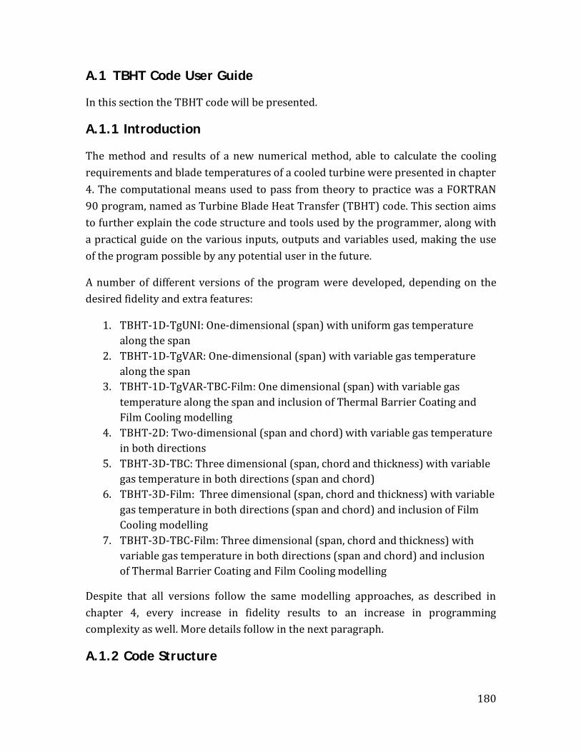
180
A.1 TBHT Code User Guide
In this section the TBHT code will be presented.
A.1.1 Introduction
The method and results of a new numerical method, able to calculate the cooling requirements and blade temperatures of a cooled turbine were presented in chapter 4. The computational means used to pass from theory to practice was a FORTRAN 90 program, named as Turbine Blade Heat Transfer (TBHT) code. This section aims to further explain the code structure and tools used by the programmer, along with a practical guide on the various inputs, outputs and variables used, making the use of the program possible by any potential user in the future.
A number of different versions of the program were developed, depending on the desired fidelity and extra features:
1. TBHT-1D-TgUNI: One-dimensional (span) with uniform gas temperature along the span
2. TBHT-1D-TgVAR: One-dimensional (span) with variable gas temperature along the span
3. TBHT-1D-TgVAR-TBC-Film: One dimensional (span) with variable gas temperature along the span and inclusion of Thermal Barrier Coating and Film Cooling modelling
4. TBHT-2D: Two-dimensional (span and chord) with variable gas temperature in both directions
5. TBHT-3D-TBC: Three dimensional (span, chord and thickness) with variable gas temperature in both directions (span and chord)
6. TBHT-3D-Film: Three dimensional (span, chord and thickness) with variable gas temperature in both directions (span and chord) and inclusion of Film Cooling modelling
7. TBHT-3D-TBC-Film: Three dimensional (span, chord and thickness) with variable gas temperature in both directions (span and chord) and inclusion of Thermal Barrier Coating and Film Cooling modelling
Despite that all versions follow the same modelling approaches, as described in chapter 4, every increase in fidelity results to an increase in programming complexity as well. More details follow in the next paragraph.
A.1.2 Code Structure
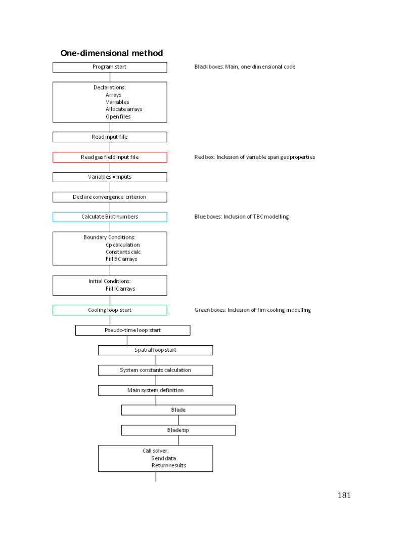
181
One-dimensional method
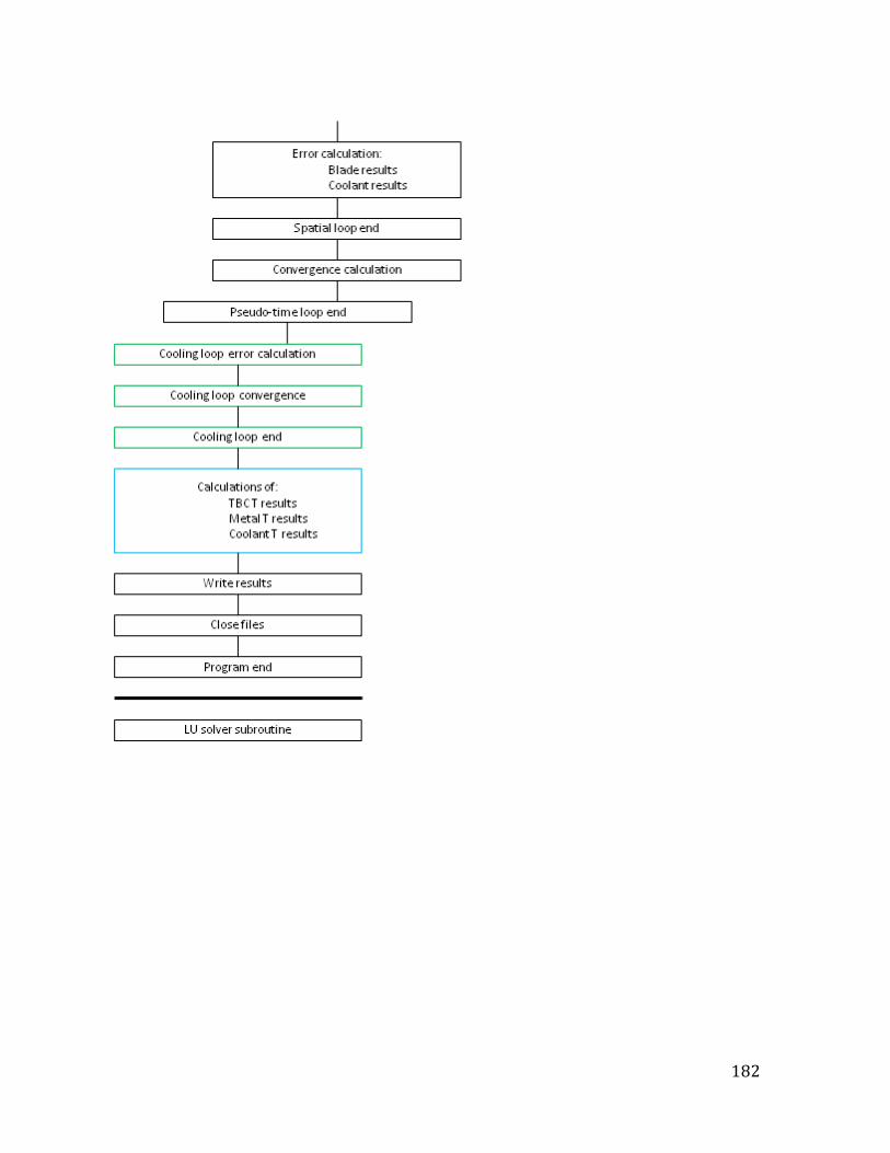
182
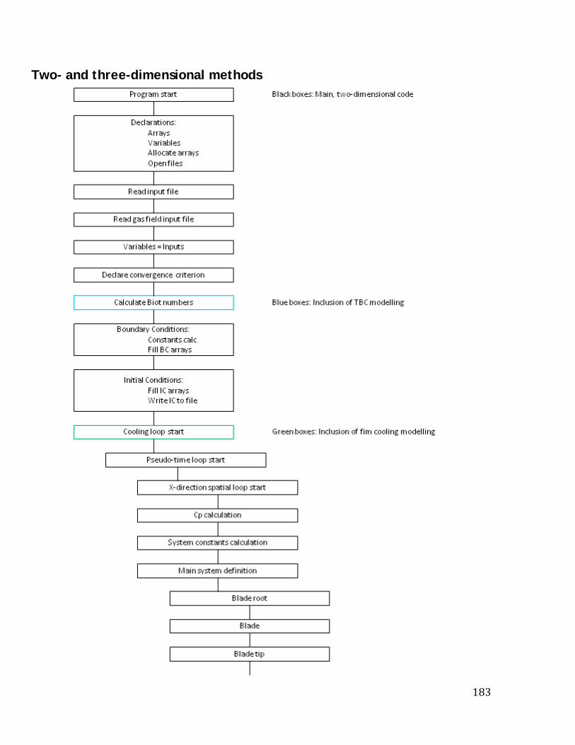
183
Two- and three-dimensional methods
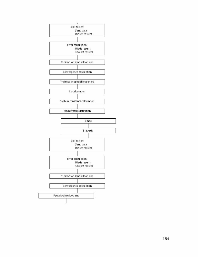
184
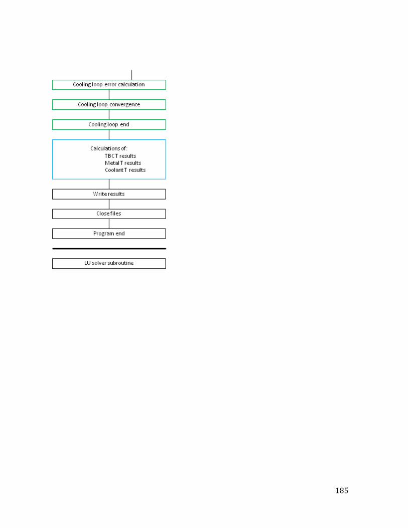
185
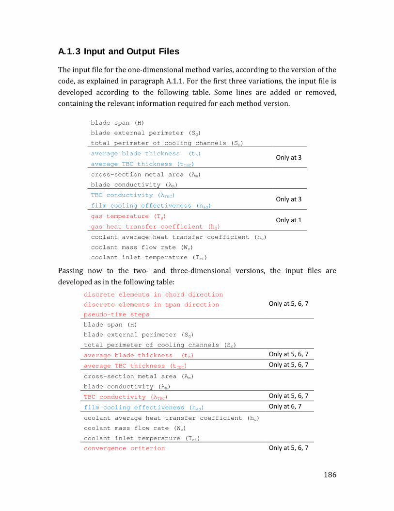
186
A.1.3 Input and Output Files
The input file for the one-dimensional method varies, according to the version of the code, as explained in paragraph A.1.1. For the first three variations, the input file is developed according to the following table. Some lines are added or removed, containing the relevant information required for each method version.
blade span (H)
blade external perimeter (Sg)
total perimeter of cooling channels (Sc)
average blade thickness (tb) Only at 3 average TBC thickness (tTBC)
cross-section metal area (Am)
blade conductivity (λm)
TBC conductivity (λTBC) Only at 3 film cooling effectiveness (nad)
gas temperature (Tg) Only at 1 gas heat transfer coefficient (hg)
coolant average heat transfer coefficient (hc)
coolant mass flow rate (Wc)
coolant inlet temperature (Tci)
Passing now to the two- and three-dimensional versions, the input files are developed as in the following table:
discrete elements in chord direction
Only at 5, 6, 7 discrete elements in span direction
pseudo-time steps
blade span (H)
blade external perimeter (Sg)
total perimeter of cooling channels (Sc)
average blade thickness (tb) Only at 5, 6, 7 average TBC thickness (tTBC) Only at 5, 6, 7 cross-section metal area (Am)
blade conductivity (λm)
TBC conductivity (λTBC) Only at 5, 6, 7 film cooling effectiveness (nad) Only at 6, 7 coolant average heat transfer coefficient (hc)
coolant mass flow rate (Wc)
coolant inlet temperature (Tci)
convergence criterion Only at 5, 6, 7

187
For the code versions requiring the gas state as input (2-7), an additional input file is needed, named “gas_state.dat” and containing two columns: The first column represents the gas temperature field and the second column the heat transfer coefficient. For the one-dimensional cases, this includes all span values, from hub to tip. For the two- and three-dimensional cases, the inputs should be first for every chord element at the hub position and then proceeding with increasing span.
Passing to output files, the programs return the following files, according to each version:
1 Boundary and Initial conditions
2 Full results, all iterations
3 System solver information
4 Convergence progress
5 Short results
6 Temperatures for all layers Only at 3, 5, 7 7
8 Average film temperature Only at 3, 6, 7
The format of the output files follows the same of the input files: First come the chord results and then they repeat for every span position.


![Numerical and Analytical Modelling of Battery Thermal ... · Cooling plate geometry (cooling channel in black) and optimized designs [32]. .....42 Fig. 22. Temperature distributions](https://img.pdfslide.us/doc/110x75/5f69337dd1fb9c42054efdd7/numerical-and-analytical-modelling-of-battery-thermal-cooling-plate-geometry.jpg)