Embed Size (px)
Citation preview

TU Delft MSc “Spaceflight”
Entrance Test Study Material For the Academic Year 2021-2022

Table of Contents :
1. Instructions & Background Information ..................................................... I
2. Satellite Orbits: Part 1 ............................................................................... 1
3. Satellite Orbits: Part 2 ............................................................................. 50
4. Space Environment ................................................................................. 75
5. Ground Systems and Operations ........................................................... 103
6. Spacecraft Design .................................................................................. 121
6.1 Steps in spacecraft requirements generation ................................................................. 121
6.2 Requirements on requirements generation .................................................................... 123
6.3 Spacecraft Subsystems: Thermal Control ........................................................................ 124
6.4 Spacecraft Subsystems: Electrical Power Generation ..................................................... 139
7 Launcher Design .................................................................................... 160
7.1 The rocket equation ......................................................................................................... 160
7.2 Single stage rockets ......................................................................................................... 162
7.3 Multi-stage rockets .......................................................................................................... 165
7.4 Limiting gravity loss and drag .......................................................................................... 171
8 Velocity increment needed to launch into orbit .................................... 173
9 Parametric estimation .......................................................................... 176
Appendix E: Some statistics................................................................... 181
Appendix H: Earth Satellite Parameters ................................................ 185
Appendix I: Solar System Parameters and atmospheric density ............ 186

I
1. Instructions & Background information
PLEASE READ THE FOLLOWING CAREFULLY.
This entrance exam has the purpose of ranking and selecting the next generation of MSc
Spaceflight students for the 2021-2022 academic year, who have all satisfied the entry
requirements. The exam will consists of a set of questions that will have to be answered on
the online Möbius platform. A second test will have to be made on non-cognitive skills; the
material presented in this document is meant to prepare for the first test (on cognitive
knowledge and skills) only.
The exam is considered as an ‘open-book’ exam. This means that the student is allowed to
use the study material given in this document. It is strongly advised to prepare the exam by
studying the material and by making your own formula sheet, which can be used during the
exam.
The following study material contains basic interdisciplinary and cross-curricular notions
that will be useful in approaching the most representative courses given in the Spaceflight
MSc, for both the Space Exploration and the Space Engineering profiles. We advise you to
not study the material by heart but to aim for an understanding of the material and the
mechanics around space missions and spacecraft design.
Here are a few instructions to be followed (a more specific one on technical aspects of the
exam will be circulated at a later moment in time):
• During the exam, always remember to regularly save your answers by switching
between the questions (without leaving the exam, of course). These instructions will
be repeated during the test.
• You will be required right at the end of the exam to send by email a scan/picture of
your worked out solutions. They will be looked at only in case of ambiguity or
technical issue with the Möbius software.
• Only the final answers in Möbius count for a correct result or not. The procedure
used to reach your final answer will not grant any partial points.
• You are only allowed to use the provided study material, your own formula sheet,
and a scientific calculator during the exam. Graphical calculators are allowed.
Calculators with internet access options are not allowed. Of course, the memory of
whatever calculator has to be emptied beforehand. The use of any other external
software is not allowed (e.g. Excel, Matlab, Python, etc.).
• You are not required to know all the constants used in equations by heart. Those will
be provided in each question. Equations not present in this file will also be provided
in the questions themselves.

II
• Pay attention that in the Möbius platform, the decimals are separated by a point “.”
and not a comma “,”. Please do not use the comma to separate thousands as well.
E.g. 2543.677 is a correct answer, but 2543,677 is not acceptable.

1AE1110-II Introduction to Aerospace Engineering II (Space) |
Introduction to Aerospace Engineering II (AE1110-II)
Satellite orbits (1)November 18, 2020 (v20.1)
R. Noomen, B.A.C. Ambrosius
2AE1110-II Introduction to Aerospace Engineering II (Space) |
Introduction
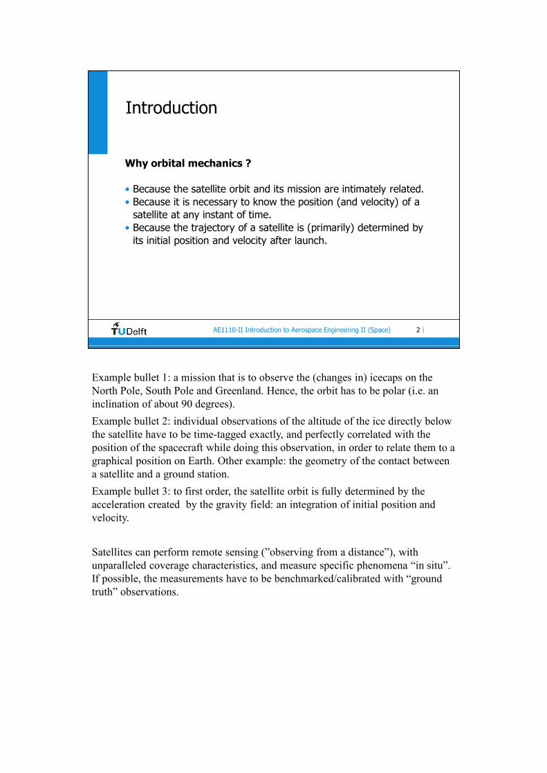
Why orbital mechanics ?
• Because the satellite orbit and its mission are intimately related.• Because it is necessary to know the position (and velocity) of a
satellite at any instant of time.• Because the trajectory of a satellite is (primarily) determined by
its initial position and velocity after launch.
Example bullet 1: a mission that is to observe the (changes in) icecaps on the North Pole, South Pole and Greenland. Hence, the orbit has to be polar (i.e. an inclination of about 90 degrees).
Example bullet 2: individual observations of the altitude of the ice directly below the satellite have to be time-tagged exactly, and perfectly correlated with the position of the spacecraft while doing this observation, in order to relate them to a graphical position on Earth. Other example: the geometry of the contact between a satellite and a ground station.
Example bullet 3: to first order, the satellite orbit is fully determined by the acceleration created by the gravity field: an integration of initial position and velocity.
Satellites can perform remote sensing (”observing from a distance”), with unparalleled coverage characteristics, and measure specific phenomena “in situ”. If possible, the measurements have to be benchmarked/calibrated with “ground truth” observations.
3AE1110-II Introduction to Aerospace Engineering II (Space) |
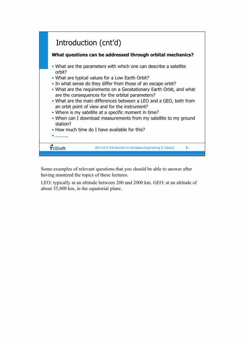
Introduction (cnt’d)What questions can be addressed through orbital mechanics?
• What are the parameters with which one can describe a satellite orbit?
• What are typical values for a Low Earth Orbit?• In what sense do they differ from those of an escape orbit?• What are the requirements on a Geostationary Earth Orbit, and what
are the consequences for the orbital parameters?• What are the main differences between a LEO and a GEO, both from
an orbit point of view and for the instrument?• Where is my satellite at a specific moment in time?• When can I download measurements from my satellite to my ground
station?• How much time do I have available for this?• ……….
Some examples of relevant questions that you should be able to answer after having mastered the topics of these lectures.
LEO: typically at an altitude between 200 and 2000 km. GEO: at an altitude of about 35,800 km, in the equatorial plane.
4AE1110-II Introduction to Aerospace Engineering II (Space) |
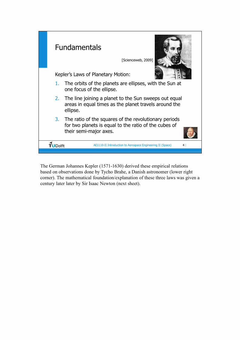
Fundamentals
Kepler’s Laws of Planetary Motion:
1. The orbits of the planets are ellipses, with the Sun at one focus of the ellipse.
2. The line joining a planet to the Sun sweeps out equal areas in equal times as the planet travels around the ellipse.
3. The ratio of the squares of the revolutionary periods for two planets is equal to the ratio of the cubes of their semi-major axes.
[Scienceweb, 2009]
The German Johannes Kepler (1571-1630) derived these empirical relations based on observations done by Tycho Brahe, a Danish astronomer (lower right corner). The mathematical foundation/explanation of these three laws was given a century later later by Sir Isaac Newton (next sheet).
5AE1110-II Introduction to Aerospace Engineering II (Space) |
Fundamentals (cnt’d)
Newton’s Laws of Motion:
1. In the absence of a force, a body either is at rest or moves in a straight line with constant speed.
2. A body experiencing a force F experiences an acceleration a related to F by F = M a, where M is the mass of the body. Alternatively, the force is proportional to the time derivative of the momentum.
3. Whenever a first body exerts a force F on a second body, the second body exerts a force −F on the first body. F and −F are equal in magnitude and opposite in direction.
Sir Isaac Newton (1643-1727), England.
Note: force F and acceleration a are written in bold, i.e. they are vectors (with a magnitude and a direction).
We use it in our daily description of physical situations: Newtonian mechanics.
6AE1110-II Introduction to Aerospace Engineering II (Space) |
Fundamentals (cnt’d)
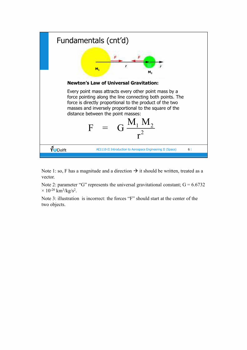
Newton’s Law of Universal Gravitation:
Every point mass attracts every other point mass by a force pointing along the line connecting both points. The force is directly proportional to the product of the two masses and inversely proportional to the square of the distance between the point masses:
1 22
M MF = G
r
M1M2
Note 1: so, F has a magnitude and a direction it should be written, treated as a vector.
Note 2: parameter “G” represents the universal gravitational constant; G = 6.6732 × 10⁻²⁰ km3/kg/s2.
Note 3: illustration is incorrect: the forces “F” should start at the center of the two objects.
7AE1110-II Introduction to Aerospace Engineering II (Space) |
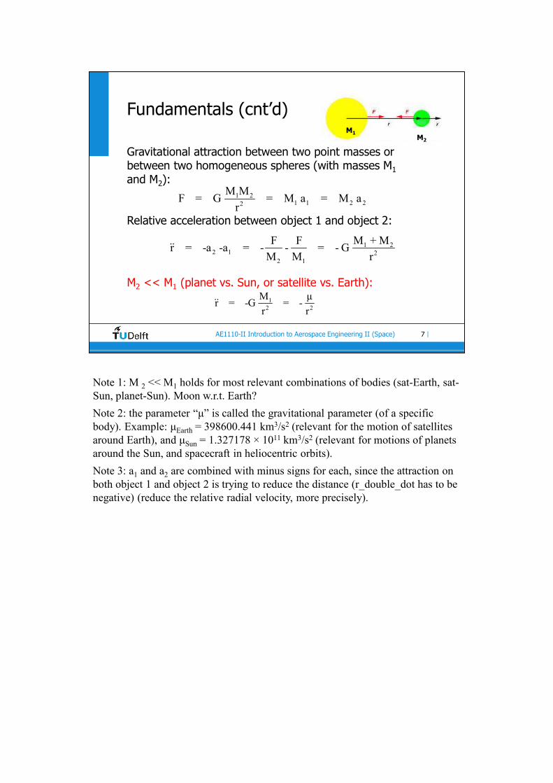
Gravitational attraction between two point masses or between two homogeneous spheres (with masses M1and M2):
Relative acceleration between object 1 and object 2:
M2 << M1 (planet vs. Sun, or satellite vs. Earth):
Fundamentals (cnt’d)
1 22 1 2
2 1
M + MF Fr = -a -a = - - = - G
M M r
1 21 1 2 22
M MF = G = M a = M a
r
12 2
M μr = -G = -
r r
M1M2
Note 1: M 2 << M1 holds for most relevant combinations of bodies (sat-Earth, sat-Sun, planet-Sun). Moon w.r.t. Earth?
Note 2: the parameter “μ” is called the gravitational parameter (of a specific body). Example: μEarth = 398600.441 km3/s2 (relevant for the motion of satellites around Earth), and μSun = 1.327178 × 10¹¹ km3/s2 (relevant for motions of planets around the Sun, and spacecraft in heliocentric orbits).
Note 3: a1 and a2 are combined with minus signs for each, since the attraction on both object 1 and object 2 is trying to reduce the distance (r_double_dot has to be negative) (reduce the relative radial velocity, more precisely).

8AE1110-II Introduction to Aerospace Engineering II (Space) |
Relative acceleration:
1D case:
Conversion to 3D case (vector notation):
General equation of motion for satellites, planets and moons
Fundamentals (cnt’d)
2
μr = -
r
2 3 3
x xμ μ μ
= - = - or y = - yr r r r
z z
rr r
M1M2
x
y
Note: the vector r can easily be decomposed into its cartesian components x, y and z; the same can be done for the radial acceleration.
Equation of motion for (1) satellites and Moon orbiting around Earth, (2) satellites, planets, asteroids and comets orbiting around the Sun, and (3) moons orbiting around (other) planets.

9AE1110-II Introduction to Aerospace Engineering II (Space) |
Numerical example acceleration
Question:
Consider the Earth (GM = μ = 398600.441 km3/s2; Re = 6378.136 km).What is (the absolute value of) the gravitational acceleration?
1. at sea surface2. for an earth-observation satellite at 800 km altitude3. for a GPS satellite at 20,200 km altitude4. for a geostationary satellite at 35,800 km altitude
Answers: see footnotes below (BUT TRY YOURSELF FIRST!)
Answers (DID YOU TRY?):
1. 9.798 m/s2
2. 7.736 m/s2
3. 0.564 m/s2
4. 0.224 m/s2
10AE1110-II Introduction to Aerospace Engineering II (Space) |
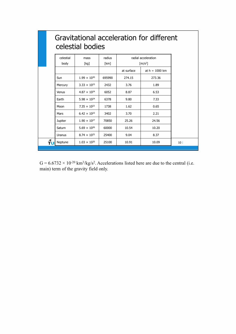
Gravitational acceleration for different celestial bodies
celestial
body
mass
[kg]
radius
[km]
radial acceleration
[m/s2]
at surface at h = 1000 km
Sun 1.99 × 1030 695990 274.15 273.36
Mercury 3.33 × 10²³ 2432 3.76 1.89
Venus 4.87 × 1024 6052 8.87 6.53
Earth 5.98 × 1024 6378 9.80 7.33
Moon 7.35 × 10²² 1738 1.62 0.65
Mars 6.42 × 10²³ 3402 3.70 2.21
Jupiter 1.90 × 1027 70850 25.26 24.56
Saturn 5.69 × 1026 60000 10.54 10.20
Uranus 8.74 × 1025 25400 9.04 8.37
Neptune 1.03 × 1026 25100 10.91 10.09
G = 6.6732 × 10⁻²⁰ km3/kg/s2. Accelerations listed here are due to the central (i.e. main) term of the gravity field only.

11AE1110-II Introduction to Aerospace Engineering II (Space) |
Numerical example acceleration (2)
1. Consider the situation of the Earth, the Sun and a satellite somewhere on the line connecting the two main bodies. Where is the point where the direct attracting forces of Earth and the Sun, acting on the satellite, are in equilibrium?Data: μEarth = 398600.441 km3/s2, μSun = 1.327178×10¹¹ km3/s2, 1 AU (average distance Earth-Sun) = 149.6×10⁶ km.Hint: make general formulation, and solve by trial-and-error.
2. The Moon orbits Earth at a distance w.r.t. the center-of-mass of Earth of about 384,000 km. Still, the Sun does not pull it away from Earth. Why not?
Answers: see footnotes below (BUT TRY YOURSELF FIRST!)
Answers (DID YOU TRY?):
1. at a distance of about 258,800 km from the center of Earth.
2. the Sun not only attracts the Moon in between, but also Earth itself, so one needs to take the difference between the two to get the net acceleration.
12AE1110-II Introduction to Aerospace Engineering II (Space) |
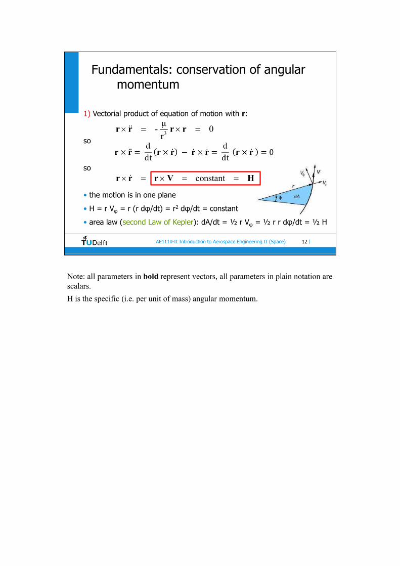
Fundamentals: conservation of angular momentum
1) Vectorial product of equation of motion with r:
so
so
• the motion is in one plane
• H = r Vφ = r (r dφ/dt) = r2 dφ/dt = constant
• area law (second Law of Kepler): dA/dt = ½ r Vφ = ½ r r dφ/dt = ½ H
3
μ- 0
r r r r r
constant r r r V H
Note: all parameters in bold represent vectors, all parameters in plain notation are scalars.
H is the specific (i.e. per unit of mass) angular momentum.

13AE1110-II Introduction to Aerospace Engineering II (Space) |
Fundamentals: conservation of energy
2) Scalar product of equation of motion with dr/dt:
or
or
Integration:
3
μ0
r r r r r
2 23 3
1 d 1 μ d 1 d 1 μ d( ) ( ) ( V ) + ( r ) 0
2 dt 2 r dt 2 dt 2 r dt r r r r
2V μ- constant E
2 r
2d 1 μV - = 0
dt 2 r
kinetic energypotential energy(incl. minus sign!)
Note 1: the step from (1/2) (μ/r3) d(r2)/dt to d(–μ/r)/dt is not a trivial one (if only for the change of sign….).
Note 2: Here, kinetic, potential and total energy are specific energies, i.e. per unit of mass.
Note 3: making a linearisation of the expression for potential energy, with the Earth’s surface as the reference and only taking terms that are constant and/or linear in altitude h, will yield the classical high-school expression E_potential = g*h (per unit of mass): Epot,h – Epot,0 = -μ/(RE+h) – (-μ/RE) ~ (μ/(RE)2 * h = g0 * h.

14AE1110-II Introduction to Aerospace Engineering II (Space) |
Fundamentals: orbit equation
3) Scalar product of equation of motion with r:
Therefore:
Note that
so:
Substitution of
yields:
3
μ0
r r r r r
d μ( ) ( ) 0
dt r r r r r
2rr V = rr and V r r r V r r V V
2 2 μr r + r - V + = 0
r
2 2 2 2 2r φV = V + V = r + ( r φ )
22
μr - r φ = -
r
Note 1: we managed to get rid of the vector notations, and are left with scalar parameters only.
Note 2: Vr is the magnitude of the radial component of the velocity, Vφ is that of the transverse component of the velocity (together forming the total velocity (vector) V).
15AE1110-II Introduction to Aerospace Engineering II (Space) |
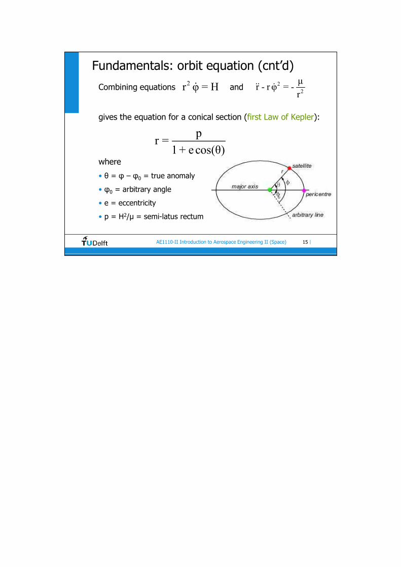
Fundamentals: orbit equation (cnt’d)
Combining equations and
gives the equation for a conical section (first Law of Kepler):
where
• θ = φ – φ0 = true anomaly
• φ0 = arbitrary angle
• e = eccentricity
• p = H2/μ = semi-latus rectum
22
μr - r φ = -
r 2r φ = H
pr =
1 + e cos(θ)
16AE1110-II Introduction to Aerospace Engineering II (Space) |
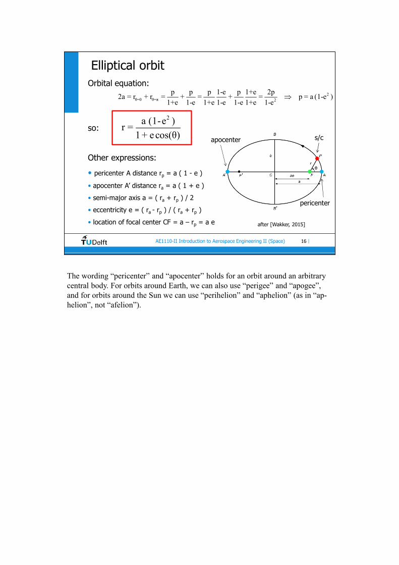
Elliptical orbitOrbital equation:
so:
Other expressions:
• pericenter A distance rp = a ( 1 - e )
• apocenter A’ distance ra = a ( 1 + e )
• semi-major axis a = ( ra + rp ) / 2
• eccentricity e = ( ra - rp ) / ( ra + rp )
• location of focal center CF = a – rp = a e
2θ=0 θ=π 2
p p p 1-e p 1+e 2p2a = r + r = + = + = p = a (1-e )
1+e 1-e 1+e 1-e 1-e 1+e 1-e
2a (1-e )r =
1 + e cos(θ)
after [Wakker, 2015]
pericenter
apocenter s/c
The wording “pericenter” and “apocenter” holds for an orbit around an arbitrary central body. For orbits around Earth, we can also use “perigee” and “apogee”, and for orbits around the Sun we can use “perihelion” and “aphelion” (as in “ap-helion”, not “afelion”).
17AE1110-II Introduction to Aerospace Engineering II (Space) |
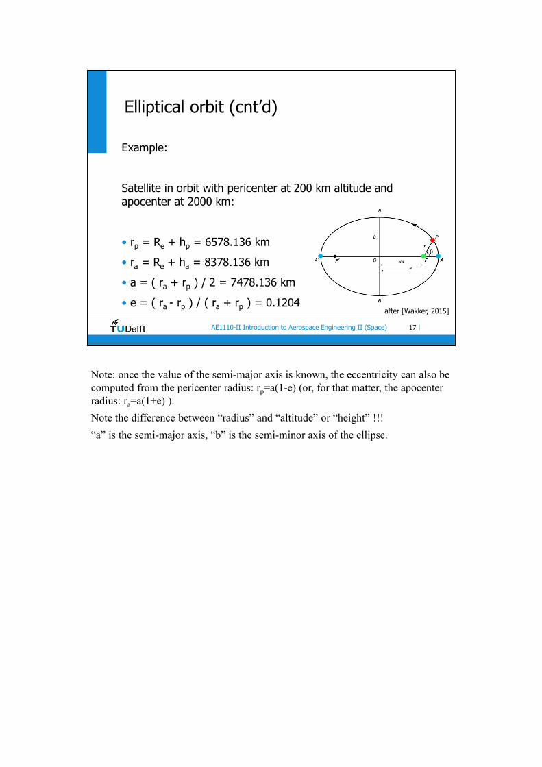
Example:
Satellite in orbit with pericenter at 200 km altitude and apocenter at 2000 km:
• rp = Re + hp = 6578.136 km
• ra = Re + ha = 8378.136 km
• a = ( ra + rp ) / 2 = 7478.136 km
• e = ( ra - rp ) / ( ra + rp ) = 0.1204
Elliptical orbit (cnt’d)
after [Wakker, 2015]
Note: once the value of the semi-major axis is known, the eccentricity can also be computed from the pericenter radius: rp=a(1-e) (or, for that matter, the apocenter radius: ra=a(1+e) ).
Note the difference between “radius” and “altitude” or “height” !!!
“a” is the semi-major axis, “b” is the semi-minor axis of the ellipse.
18AE1110-II Introduction to Aerospace Engineering II (Space) |
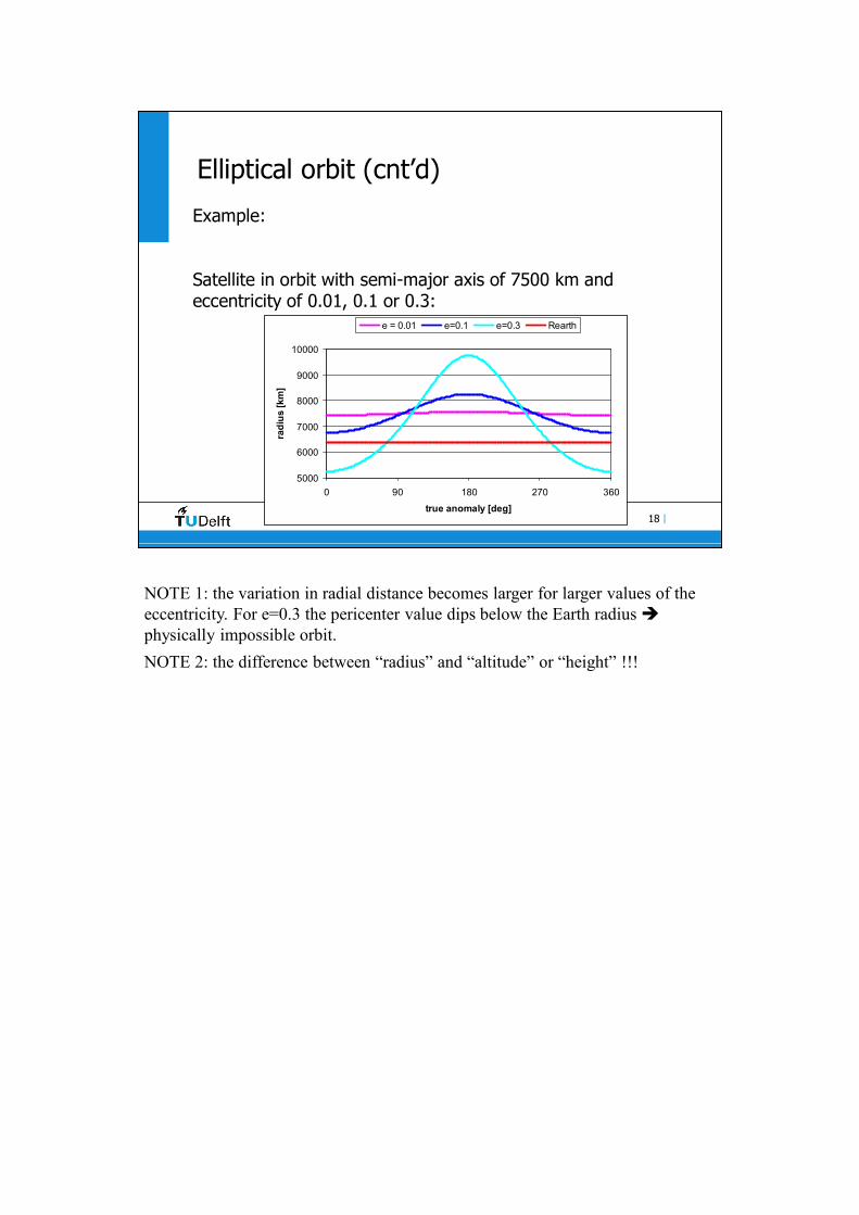
Example:
Satellite in orbit with semi-major axis of 7500 km and eccentricity of 0.01, 0.1 or 0.3:
Elliptical orbit (cnt’d)
5000
6000
7000
8000
9000
10000
0 90 180 270 360
true anomaly [deg]
rad
ius
[km
]
e = 0.01 e=0.1 e=0.3 Rearth
NOTE 1: the variation in radial distance becomes larger for larger values of the eccentricity. For e=0.3 the pericenter value dips below the Earth radius physically impossible orbit.
NOTE 2: the difference between “radius” and “altitude” or “height” !!!

19AE1110-II Introduction to Aerospace Engineering II (Space) |
Elliptical orbit: velocity and energy
pp p a a a p
a
2 2p a
p a
p a a
2p
2a
conservation of angular momentum:
rH = r V = r V V = V
r
conservation of energy:
1 μ 1 μE = V - = V -
2 r 2 r
substituting r , r , V yields:
μ 1+eV =
a 1-e
and
μ 1-eV =
a 1+ e
Straightforward derivation of simple relations for the velocity at pericenter and apocenter.
20AE1110-II Introduction to Aerospace Engineering II (Space) |
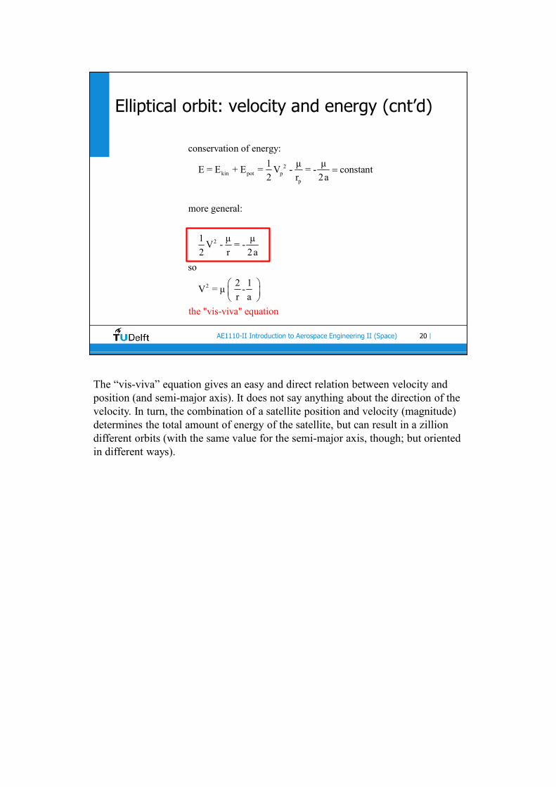
Elliptical orbit: velocity and energy (cnt’d)
2kin pot p
p
2
2
conservation of energy:
1 μ μE = E + E = V - = - constant
2 r 2a
more general:
1 μ μV - = -
2 r 2a
so
2 1V = μ -
r a
the "vis-viva" equation
The “vis-viva” equation gives an easy and direct relation between velocity and position (and semi-major axis). It does not say anything about the direction of the velocity. In turn, the combination of a satellite position and velocity (magnitude) determines the total amount of energy of the satellite, but can result in a zillion different orbits (with the same value for the semi-major axis, though; but oriented in different ways).
21AE1110-II Introduction to Aerospace Engineering II (Space) |
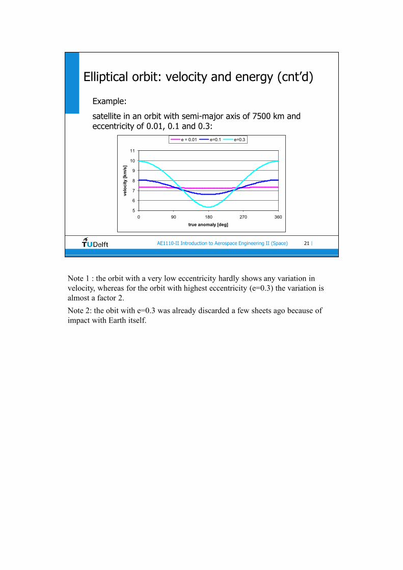
Elliptical orbit: velocity and energy (cnt’d)
Example:
satellite in an orbit with semi-major axis of 7500 km and eccentricity of 0.01, 0.1 and 0.3:
5
6
7
8
9
10
11
0 90 180 270 360
true anomaly [deg]
ve
loc
ity
[k
m/s
]
e = 0.01 e=0.1 e=0.3
Note 1 : the orbit with a very low eccentricity hardly shows any variation in velocity, whereas for the orbit with highest eccentricity (e=0.3) the variation is almost a factor 2.
Note 2: the obit with e=0.3 was already discarded a few sheets ago because of impact with Earth itself.

22AE1110-II Introduction to Aerospace Engineering II (Space) |
Area law (Kepler’s second equation):
Also:
leads to Kepler’s third law:
Elliptical orbit: orbital period
T T T
0 0 0
dA 1 dA 1 1 1= H constant A = dA = dt = H dt = H dt = H T = π a b
dt 2 dt 2 2 2
2 2b = a 1-e and H = μ p and p = a (1-e )
3aT = 2 π
μ
Important conclusion: the orbital period in an elliptical orbit “T” is fully determined by the value of the semi-major axis “a” and the gravitational parameter “μ”; the shape of the orbit (as indicated by the eccentricity “e”) does NOT play a role here!
“a” the semi-major axis, “b” is the semi-minor axis of an ellipse.
23AE1110-II Introduction to Aerospace Engineering II (Space) |
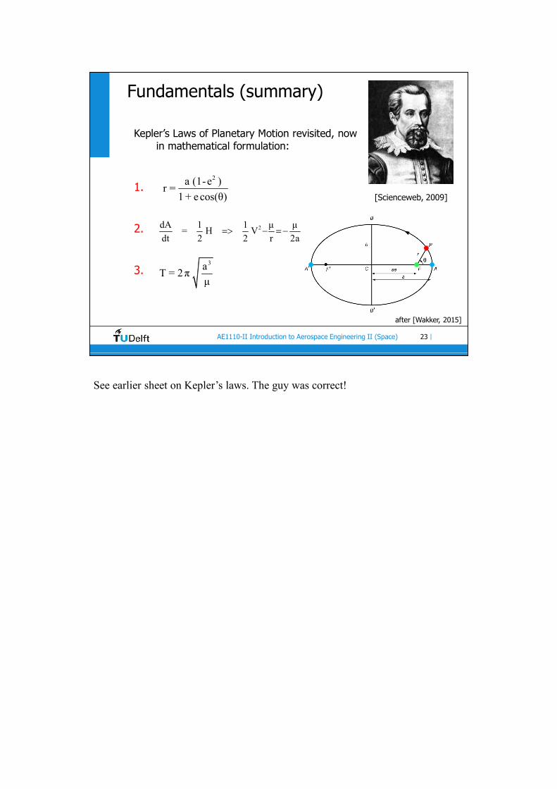
Kepler’s Laws of Planetary Motion revisited, now in mathematical formulation:
1.
2.
3.
Fundamentals (summary)
3aT = 2 π
μ
2a (1-e )r =
1 + e cos(θ) [Scienceweb, 2009]
2dA 1 1 μ μ= H V
dt 2 2 r 2a
after [Wakker, 2015]
See earlier sheet on Kepler’s laws. The guy was correct!
24AE1110-II Introduction to Aerospace Engineering II (Space) |
Elliptical orbit: example
Orbit around Earth, hp = 300 km, ha = 10000 km
Questions: a? e? Vp? Va? T?
Answers: see footnotes below (TRY FIRST !)
Data: Rearth = 6378.136 km, μearth = 398600.441 km3/s2
Answers: (DID YOU TRY?)
• rp = Rearth + hp = 6678.136 km
• ra = Rearth + ha = 16378.136 km
• a = (rp+ra)/2 = 11528.136 km
• e = (ra-rp)/(ra+rp) = 0.4207
• Vp = 9.209 km/s
• Va = 3.755 km/s
• T = 12318.3 s = 205.3 min

25AE1110-II Introduction to Aerospace Engineering II (Space) |
Elliptical orbit: position vs. time
Questions:• where is the satellite at a specific moment in time?• when is the satellite at a specific position?
Why?• to aim the antenna of a ground station• to initiate an engine burn at the proper point in orbit• to perform certain measurements at specific locations• to time-tag measurements• to be able to rendez-vous• …….

26AE1110-II Introduction to Aerospace Engineering II (Space) |
Elliptical orbit: position vs. time (cnt’d)
2 2
2
θ3
20
straightforward approach:
dθ H r r= dt = dθ Δt = dt = dθ
dt r H Hso
p dθΔt =
μ (1+ ecosθ)
difficult relation
introduce new parameter E
("eccentric anomaly")
Option 1: integrate numerically X
The straightforward approach is clear but leads to a difficult integral (see next sheet).

27AE1110-II Introduction to Aerospace Engineering II (Space) |
Elliptical orbit: position vs. time (cnt’d)
2 2
2
θ3
20
straightforward approach:
dθ H r r= dt = dθ Δt = dt = dθ
dt r H Hso
p dθΔt =
μ (1+ ecosθ)
difficult relation
introduce new parameter E
("eccentric anomaly")
after [Wakker, 2015]
Option 3
The straightforward approach is clear but leads to a difficult integral (see next sheet).
Another option: treat it numerically, but then one might just as well give up the idea of using Kepler orbits and switch to numerical representations altogether.
Yet another option (pursued here): introduce new parameter E – not to be confused with E (“energy”)!! This will be the best option to also do reverse calculations.

28AE1110-II Introduction to Aerospace Engineering II (Space) |
Elliptical orbit: position vs. time (cnt’d)
2
2
2 2 2 2 2 2 2 2
plot:
r cosθ = a cos E - a e
ellipse:
GP b= = 1-e
GP' a
here:
GP r sin θ=
GP' a sin E
or
r sin θ = a 1-e sin E
combining:
(r cos θ) + (r sin θ) = r = (a cos E -a e) + (a 1-e sin E) = a (1-e cos E)
or (r>0):
(1 cos )r a e E
after [Wakker, 2015]
P’ and the eccentric anomaly E are related to a perfect circle with radius “a”. E and θ are related to each other.
Question: what do we get if the orbit is a perfect circle (e=0)?
Distance CF is equal to “ae” since distance CA is equal to “a” and distance FA is equal to “a(1-e)”.
“a” is semi-major axis, “b” is semi-minor axis of ellipse.

29AE1110-II Introduction to Aerospace Engineering II (Space) |
Elliptical orbit: position vs. time (cnt’d)2a (1-e )
r = = a (1-e cos E)1+e cosθ
from which
θ 1+ e Etan = tan
2 1-e 2
e.g. e=0.6 :
0
90
180
270
360
0 90 180 270 360
eccentric anomaly [deg]
tru
e a
no
ma
ly [d
eg
]
The relation between E and θ is unambiguous. The derivation of this relation between tan(θ/2) and tan(E/2) is tedious…..

30AE1110-II Introduction to Aerospace Engineering II (Space) |
Elliptical orbit: position vs. time (cnt’d)
E [°] E/2 [°] θ/2 [°] θ [°]
80 40 52.04 104.08
100 50 61.22 122.44
170 85 86.72 173.44
190 95 93.28 186.56
260 130 118.78 237.56
280 140 127.96 255.92
350 175 172.39 344.78
Some numerical examples, for e=0.4 :
Verify!
Verify!

31AE1110-II Introduction to Aerospace Engineering II (Space) |
Elliptical orbit: position vs. time (cnt’d)
2
2
2
a (1-e ) μ esin θr = so r =
1+ ecosθ μ a (1-e )
and
r = a (1-e cos E) so r = a e E sin E
(all derivatives taken after time t)
r sin θequating and using = 1-e
a sin E
(continued on next page)
after [Wakker, 2015]
Second step in derivation of required relation.
DO practice your analytical skills, and make the derivation/differentiations!
32AE1110-II Introduction to Aerospace Engineering II (Space) |
Elliptical orbit: position vs. time (cnt’d)
3
3
p p3
μ 1E =
a 1-ecos E
or
μ(1-ecos E)dE = dt
aintegration:
μE -esin E = (t - t ) = n (t - t ) = M
aor
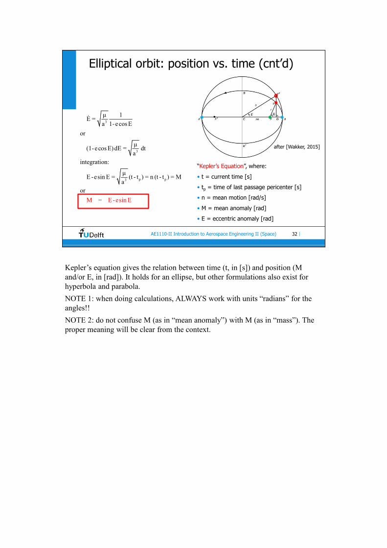
M = E -esin E
“Kepler’s Equation”, where:
• t = current time [s]
• tp = time of last passage pericenter [s]
• n = mean motion [rad/s]
• M = mean anomaly [rad]
• E = eccentric anomaly [rad]
after [Wakker, 2015]
Kepler’s equation gives the relation between time (t, in [s]) and position (M and/or E, in [rad]). It holds for an ellipse, but other formulations also exist for hyperbola and parabola.
NOTE 1: when doing calculations, ALWAYS work with units “radians” for the angles!!
NOTE 2: do not confuse M (as in “mean anomaly”) with M (as in “mass”). The proper meaning will be clear from the context.

33AE1110-II Introduction to Aerospace Engineering II (Space) |
Elliptical orbit: position vs. time (cnt’d)Example position time:
Question:
• a = 7000 km
• e = 0.1
• μ = 398600.441 km3/s2
• θ = 35°
• t-tp ?
Answer:
• n = 1.078008 × 10⁻³ rad/s
• θ = 0.61087 rad
• E = 0.55565 rad
• M = 0.50290 rad
• t-tp = 466.5 sverify!
after [Wakker, 2015]
Straightforward application of recipe. DO YOUR CALCULATIONS IN RADIANS!
34AE1110-II Introduction to Aerospace Engineering II (Space) |
Elliptical orbit: position vs. time (cnt’d)
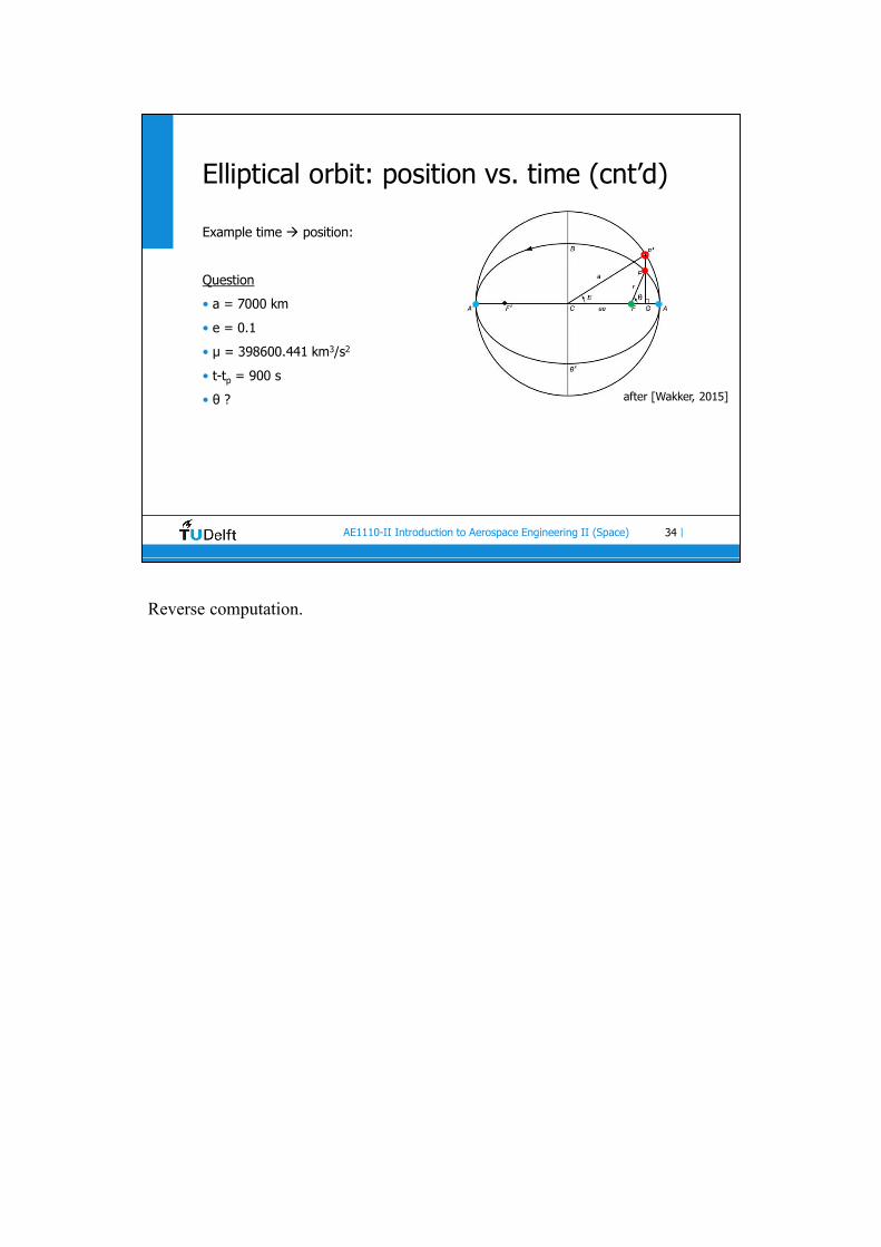
Example time position:
Question
• a = 7000 km
• e = 0.1
• μ = 398600.441 km3/s2
• t-tp = 900 s
• θ ? after [Wakker, 2015]
Reverse computation.
35AE1110-II Introduction to Aerospace Engineering II (Space) |
Elliptical orbit: position vs. time (cnt’d)
Example time position (cnt’d):
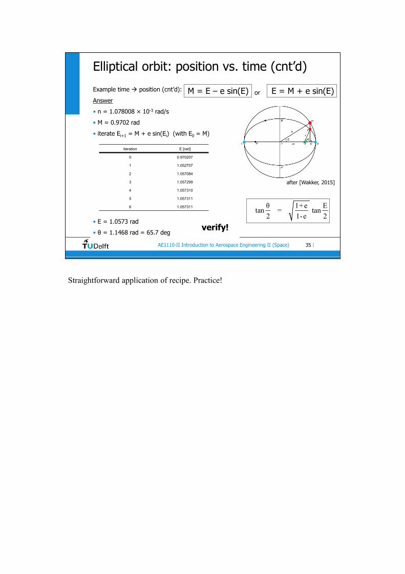
Answer
• n = 1.078008 × 10⁻³ rad/s
• M = 0.9702 rad
• iterate Ei+1 = M + e sin(Ei) (with E0 = M)
• E = 1.0573 rad
• θ = 1.1468 rad = 65.7 degverify!
iteration E [rad]
0 0.970207
1 1.052707
2 1.057084
3 1.057299
4 1.057310
5 1.057311
6 1.057311 θ 1+e Etan = tan
2 1-e 2
M = E – e sin(E)
after [Wakker, 2015]
E = M + e sin(E)or
Straightforward application of recipe. Practice!

36AE1110-II Introduction to Aerospace Engineering II (Space) |
Example elliptical orbitQuestion:
Consider a satellite at 800 km altitude above the Earth’s surface, with a transversal velocity (i.e., perpendicular to the radius) of 8 km/s. There is no radial velocity component.
1. compute the semi-major axis
2. compute the eccentricity
3. compute the maximum radius of this orbit
4. compute the maximum altitude
Data: Re = 6378.136 km, μearth = 398600.441 km3/s2
Answers:
1. 0.5 V2 – μ/r = - μ/2a a = 8470.120 km
2. Vcirc = 7.45 km/s < 8 km/s rp = a(1-e) e = 0.1525
3. ra = a(1+e) ra = 9762.105 km
4. h = r-Re hmax = 3383.969 km
Verify !!
Straightforward application of recipe. Practice!
Question 2: first compute the circular velocity. If the velocity of the s/c is equal to this circular velocity, it is in a circular orbit (obviously). If the velocity is smaller than Vc, the s/c does not have enough energy to sustain a circular orbit and falls back to Earth: the current position is the apocenter. If the velocity is larger than Vc, (as is the case in this specific question), the s/c travels out to larger distances and at this moment must be in pericenter of the orbit…. So we apply the expression for rp.

37AE1110-II Introduction to Aerospace Engineering II (Space) |
Example elliptical orbit
Question:
Consider a satellite at 800 km altitude above the Earth’s surface, with a transversal velocity (i.e., perpendicular to the radius) of 10 km/s. There is no radial velocity component.
1. compute the semi-major axis
2. compute the eccentricity
3. compute the maximum radius of this orbit
4. compute the maximum altitude
Answers: see footnotes below (BUT TRY YOURSELF FIRST!!)
Answers: (DID YOU TRY FIRST??)
1. a = 36041.140 km
2. e = 0.8008
3. ra = 64904.145 km
4. hmax = 58526.009 km
38AE1110-II Introduction to Aerospace Engineering II (Space) |
Orbits: types
Shape of trajectory and energy are directly related
Experiment
Newton’s cannon [www.waoven.screaming.net, 2017]
Total amount of specific energy = -μ/2a.
39AE1110-II Introduction to Aerospace Engineering II (Space) |
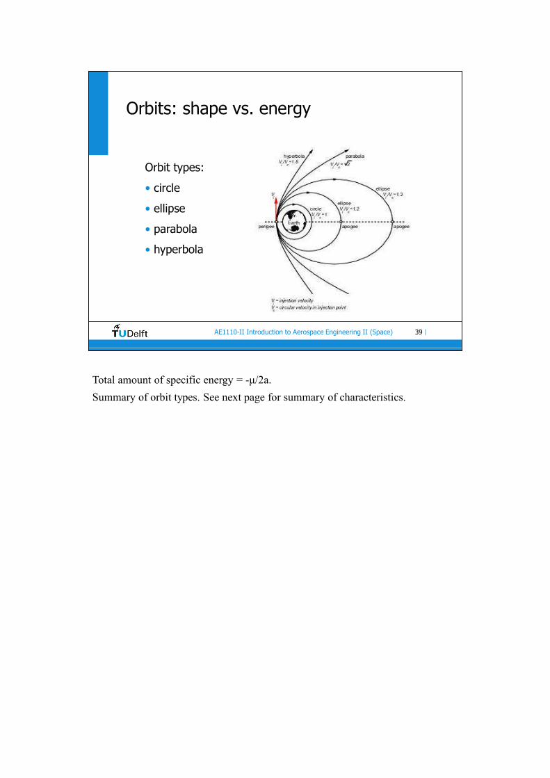
Orbits: shape vs. energy
Orbit types:
• circle
• ellipse
• parabola
• hyperbola
Total amount of specific energy = -μ/2a.
Summary of orbit types. See next page for summary of characteristics.

40AE1110-II Introduction to Aerospace Engineering II (Space) |
Circular orbit
Characteristics:
• e = 0
• rmin = rmax = r
• r = a
• V = Vc = √ (μ/a)
• T = 2 π √ (a3/μ)
• Etot = - μ/2a < 0
after [real-world-physics-problems.com, 2014]
r
Some characteristics of circular orbits. The expressions can be easily verified by substituting e=0 in the general equations derived for an ellipse (with 0<e<1).
IMPORTANT: the length of “r” is measured from the center of Earth, NOT the surface!

41AE1110-II Introduction to Aerospace Engineering II (Space) |
Circular orbit (cnt’d)
The orbital velocity at low altitudes is 7-7.9 km/s, but at higher altitudes it reduces quickly (notice logarithmic scale for altitude). The reverse happens with the orbital period. In the case of a circular orbit (only then!), the orbital period T and the velocity V are related to each other by the equation T V = 2πr = 2πa. Do not confuse altitude (i.e. w.r.t. surface of central body) and radius (i.e. w.r.t. center of mass of central body).

42AE1110-II Introduction to Aerospace Engineering II (Space) |
Geostationary orbit
Requirements:
• Stationary (i.e. non-moving) w.r.t. Earth surface• orbital period = 23 hour, 56 min and 4 sec
• moves in equatorial plane
• moves in eastward direction
• So: orbital elements:• e = 0
• a = 42164.17 km
• i = 0°
• and:• h = a – Re = 35786 km
• Vc = 3.075 km/s
• E = - 4.727 km2/s2
[Sque, 2009]:
“geo” “stationary” as in “Earth” “fixed”. The orbital period is related to the revolution of Earth w.r.t. an inertial system, i.e. the stars -> use 23h56m4s instead of our everyday-life 24 hrs = 86400 s.
The value of ”a” is derived from the expression for the orbital period for a perfectly round and homogeneous Earth. In reality, the effect of flattening on Earth needs to be added, which causes the real altitude of the GEO to be about 522 m higher.

43AE1110-II Introduction to Aerospace Engineering II (Space) |
Geostationary orbit (cnt’d)
Questions:
Consider an obsolete GEO satellite which is put into a graveyard orbit: 300 km above the standard GEO altitude.
1. What is the orbital period of this graveyard orbit?2. What is the eccentricity of the transfer orbit that takes a satellite
from GEO to this graveyard orbit?
Data: μearth = 398600.441 km3/s2
Answers: see footnotes below BUT TRY FIRST !!
Answers:
1) T = 24 hrs, 11 min and 25.3 sec.
2) e = 0.00354

44AE1110-II Introduction to Aerospace Engineering II (Space) |
Parabolic orbit
2 2 1V = μ -
r a
pr =
1 + ecos(θ)
Characteristics:
• e = 1
• rmin = rp = p/2, rmax = ∞
• a = ∞
• V = Vesc = √ (2μ/r)
• Vmin = 0
• Tpericenterinfinity = ∞
• Etot = 0
μE = -
2a
Some characteristics of parabolic orbits. This is an “open” orbit, so there is no orbital period. The maximum distance (i.e. ∞) is achieved for θ=180°.
So: θ ranges from -180° to +180° (the trajectory has to be continuous).

45AE1110-II Introduction to Aerospace Engineering II (Space) |
Hyperbolic orbit
Characteristics:
• e > 1
• rmin = rp , rmax = ∞
• a < 0
• Vp > Vesc
• V2 = Vesc2 + V∞
2
• V∞ > 0
• Tpericenterinfinity = ∞
• Etot > 0
2a (1-e )r =
1 + e cos(θ)
2 2 1V = μ -
r a
μE = -
2a
Some characteristics of hyperbolic orbits. This is an “open” orbit, so there is no orbital period. The maximum distance (i.e. ∞) is achieved for a limiting value of θ, given by the zero crossing of the numerator of the equation for “r”: 1 + e cos(θlim) = 0. So, for a hyperbola: θ ranges between –θlim to +θlim (again, to have a continuous trajectory).
The equation for velocity (V2=Vesc2+V∞
2): consider the general vis-viva equation, and then the case where a=∞ -> expression for first term on right-hand side; the case where r goes to infinity -> expression for second term on right-hand side. Simple comme ça!
46AE1110-II Introduction to Aerospace Engineering II (Space) |
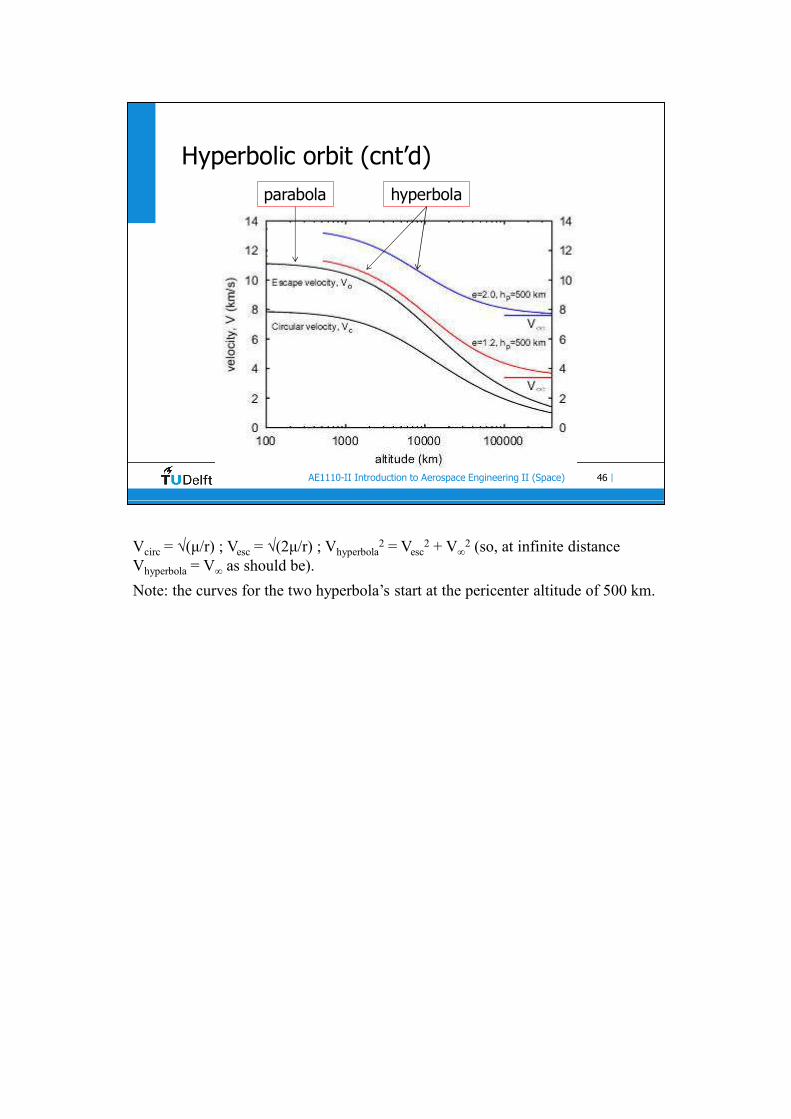
Hyperbolic orbit (cnt’d)parabola hyperbola
Vcirc = √(μ/r) ; Vesc = √(2μ/r) ; Vhyperbola2 = Vesc
2 + V∞2 (so, at infinite distance
Vhyperbola = V∞ as should be).
Note: the curves for the two hyperbola’s start at the pericenter altitude of 500 km.
47AE1110-II Introduction to Aerospace Engineering II (Space) |
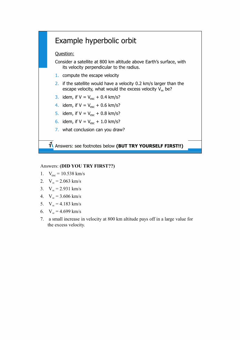
Example hyperbolic orbit
Question:
Consider a satellite at 800 km altitude above Earth’s surface, with its velocity perpendicular to the radius.
1. compute the escape velocity
2. if the satellite would have a velocity 0.2 km/s larger than the escape velocity, what would the excess velocity V∞ be?
3. idem, if V = Vesc + 0.4 km/s?
4. idem, if V = Vesc + 0.6 km/s?
5. idem, if V = Vesc + 0.8 km/s?
6. idem, if V = Vesc + 1.0 km/s?
7. what conclusion can you draw?
Answers: see footnotes below (BUT TRY YOURSELF FIRST!!)
Answers: (DID YOU TRY FIRST??)
1. Vesc = 10.538 km/s
2. V∞ = 2.063 km/s
3. V∞ = 2.931 km/s
4. V∞ = 3.606 km/s
5. V∞ = 4.183 km/s
6. V∞ = 4.699 km/s
7. a small increase in velocity at 800 km altitude pays off in a large value for the excess velocity.

48AE1110-II Introduction to Aerospace Engineering II (Space) |
Fundamentals (cnt’d)
Orbit types:
• circle
• ellipse
• parabola
• hyperbola
[Cramer, 2009]
“Conical sections”
Summary of orbit types. See next page for summary of characteristics.
49AE1110-II Introduction to Aerospace Engineering II (Space) |
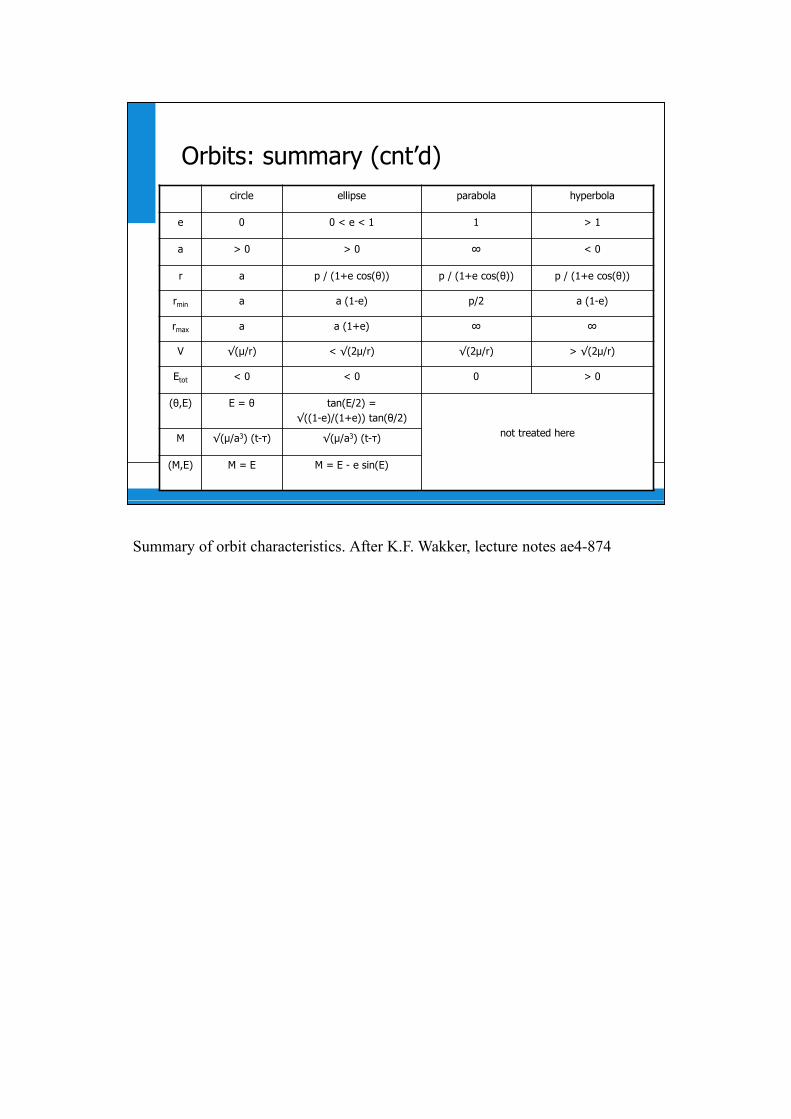
Orbits: summary (cnt’d)circle ellipse parabola hyperbola
e 0 0 < e < 1 1 > 1
a > 0 > 0 ∞ < 0
r a p / (1+e cos(θ)) p / (1+e cos(θ)) p / (1+e cos(θ))
rmin a a (1-e) p/2 a (1-e)
rmax a a (1+e) ∞ ∞
V √(μ/r) < √(2μ/r) √(2μ/r) > √(2μ/r)
Etot < 0 < 0 0 > 0
(θ,E) E = θ tan(E/2) =√((1-e)/(1+e)) tan(θ/2)
not treated hereM √(μ/a3) (t-τ) √(μ/a3) (t-τ)
(M,E) M = E M = E - e sin(E)
Summary of orbit characteristics. After K.F. Wakker, lecture notes ae4-874

50AE1110-II Introduction to Aerospace Engineering II (Space) |
Introduction to Aerospace Engineering II (AE1110-II)
Satellite orbits (2)November 19, 2020 (v20.1)
R. Noomen, B.A.C. Ambrosius

51AE1110-II Introduction to Aerospace Engineering II (Space) |
Fundamentals (two-dimensional)
three Kepler elements:• a – semi-major axis [m]• e – eccentricity [-]• tp or τ – time of pericenter passage [s]
after [Wakker, 2015]
The time of passage of a well-defined point in the orbit (e.g. the pericenter, point A) is indicated by “tp” or, equivalently, “τ” (the Greek symbol “tau”). Knowing this value, one can relate the position in the orbit to absolute time. Illustrative recap of previous lecture.
52AE1110-II Introduction to Aerospace Engineering II (Space) |
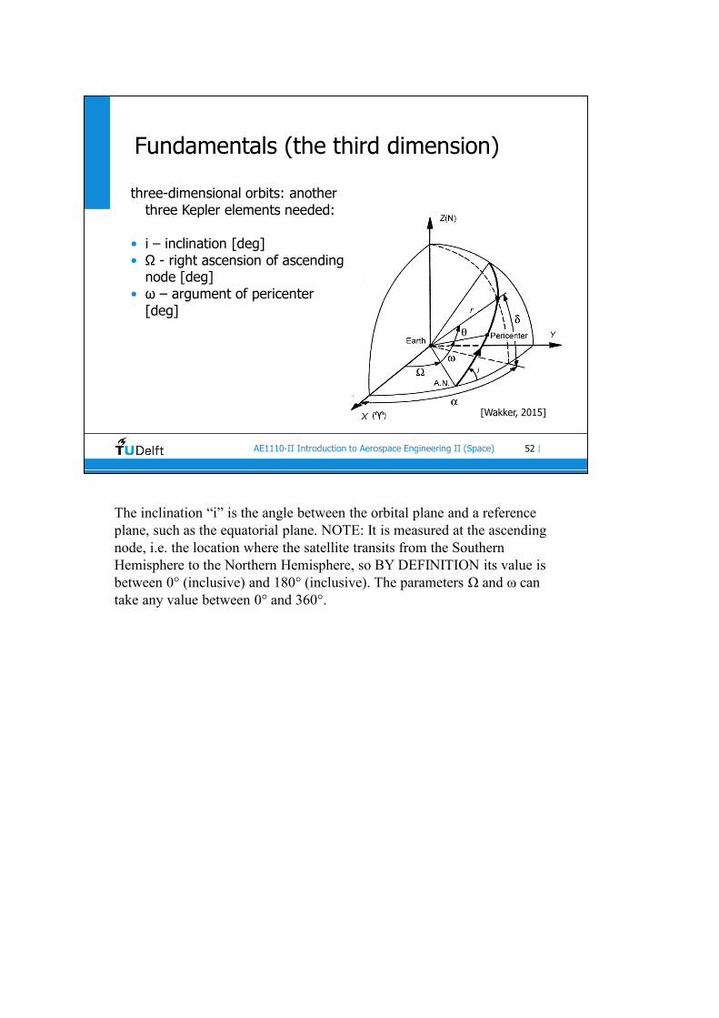
Fundamentals (the third dimension)
[Wakker, 2015]
three-dimensional orbits: another three Kepler elements needed:
• i – inclination [deg]• Ω - right ascension of ascending
node [deg]• ω – argument of pericenter
[deg]
The inclination “i” is the angle between the orbital plane and a reference plane, such as the equatorial plane. NOTE: It is measured at the ascending node, i.e. the location where the satellite transits from the Southern Hemisphere to the Northern Hemisphere, so BY DEFINITION its value is between 0° (inclusive) and 180° (inclusive). The parameters Ω and ω can take any value between 0° and 360°.
53AE1110-II Introduction to Aerospace Engineering II (Space) |
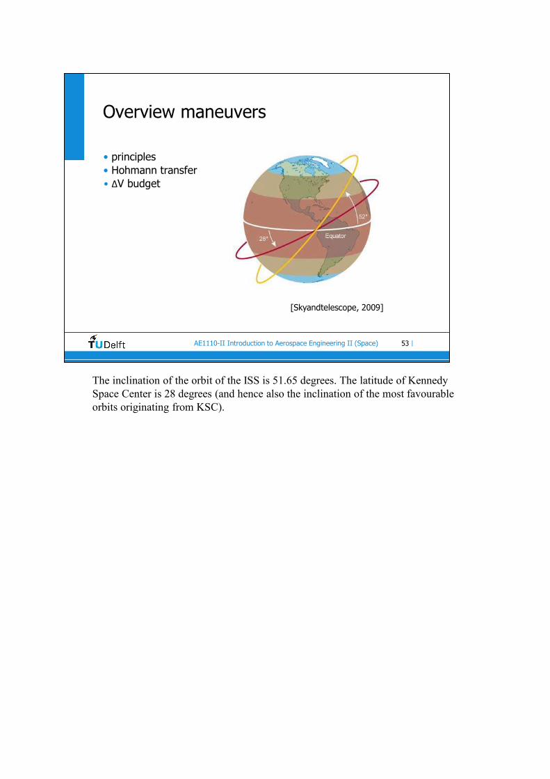
Overview maneuvers
• principles• Hohmann transfer• ΔV budget
[Skyandtelescope, 2009]
The inclination of the orbit of the ISS is 51.65 degrees. The latitude of Kennedy Space Center is 28 degrees (and hence also the inclination of the most favourable orbits originating from KSC).

54AE1110-II Introduction to Aerospace Engineering II (Space) |
Maneuvers
Purpose:• orbit transfers (e.g. LEO GTO GEO)• plane changes (e.g. launch from Kourou, with i = 5°, to
equatorial, with i = 0°)• rendez-vous• orbit maintenance
55AE1110-II Introduction to Aerospace Engineering II (Space) |
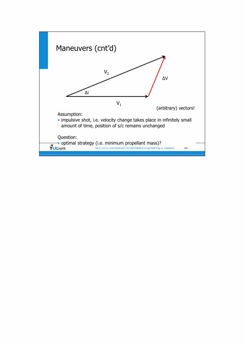
Maneuvers (cnt’d)
Assumption:• impulsive shot, i.e. velocity change takes place in infinitely small
amount of time, position of s/c remains unchanged
Question:• optimal strategy (i.e. minimum propellant mass)?
ΔV
V1
V2
Δi
(arbitrary) vectors!

56AE1110-II Introduction to Aerospace Engineering II (Space) |
Maneuvers (cnt’d)
Case 1: in-plane
2 2 22 1
V
1 1E (V V ) ( V)
2 2
2 1
2 1
1
ΔV V V
ΔV V V
V ΔV
Conclusion:• maximum energy gain for given ΔV when
o maneuver parallel to original velocityo at location where original velocity is highest
“in-plane”: the orbital plane of the s/c is not changed (only size and shape of the orbit are).
Velocity is largest in pericenter.
The dot in the third equation represents the inproduct.
57AE1110-II Introduction to Aerospace Engineering II (Space) |
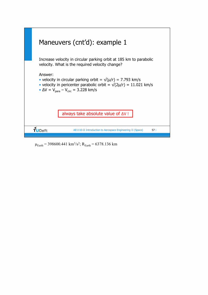
Maneuvers (cnt’d): example 1
Increase velocity in circular parking orbit at 185 km to parabolic velocity. What is the required velocity change?
Answer:• velocity in circular parking orbit = √(μ/r) = 7.793 km/s• velocity in pericenter parabolic orbit = √(2μ/r) = 11.021 km/s• ΔV = Vpara – Vcirc = 3.228 km/s
always take absolute value of ΔV !
μEarth = 398600.441 km3/s2; REarth = 6378.136 km

58AE1110-II Introduction to Aerospace Engineering II (Space) |
Maneuvers (cnt’d): example 2
Increase velocity in circular parking orbit at 185 km with 1 km/s. What is the energy gain?
Answer:• velocity in circular parking orbit = √(μ/r) = 7.793 km/s• new velocity = Vc + ΔV = 8.793 km/s• Eoriginal = ½V2 - μ/r = -30.367 km2/s2
• Enew = ½V2 - μ/r = -22.073 km2/s2
• ΔE = 8.293 km2/s2
or:• equation previous sheets: ΔE = ½(ΔV)2 + V1 • ΔV = 8.293 km2/s2
μEarth = 398600.441 km3/s2; REarth = 6378.136 km.
Two different ways to compute the energy gain (to numerically prove the expression in the second-previous sheet).
Numbers shown here may not combine exactly because of rounding.

59AE1110-II Introduction to Aerospace Engineering II (Space) |
Maneuvers (cnt’d): example 3
Increase velocity in circular parking orbit at 185 km with 1 km/s. What is the new energy? What is the new semi-major axis? What is the apocenter radius of the new orbit?
Answers:• velocity in circular parking orbit = √(μ/r) = 7.793 km/s• new velocity = Vc + ΔV = 8.793 km/s• Enew = ½V2 - μ/r = -22.073 km2/s2
• E = -μ/(2a) a = 9029 km• rp = a ( 1 – e ) e = 0.273• ra = a ( 1 + e ) = 11495 km
Same questions, after a velocity increase of 2 km/s (in the 185km orbit).• Enew = -12.780 km2/s2
• a = 15594 km• ra = 24626 km
μEarth = 398600.441 km3/s2; REarth = 6378.136 km.
Numbers shown here may not combine exactly because of rounding.
60AE1110-II Introduction to Aerospace Engineering II (Space) |
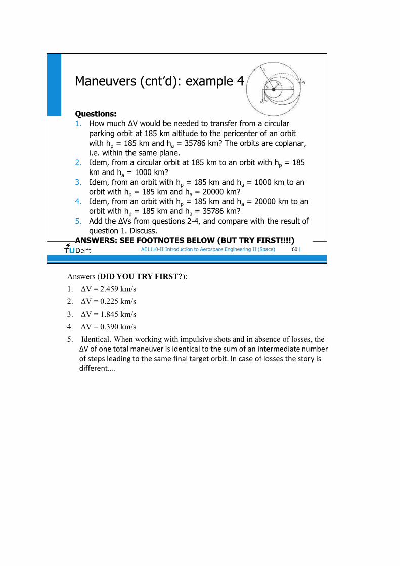
Maneuvers (cnt’d): example 4
Questions:1. How much ΔV would be needed to transfer from a circular
parking orbit at 185 km altitude to the pericenter of an orbit with hp = 185 km and ha = 35786 km? The orbits are coplanar, i.e. within the same plane.
2. Idem, from a circular orbit at 185 km to an orbit with hp = 185 km and ha = 1000 km?
3. Idem, from an orbit with hp = 185 km and ha = 1000 km to an orbit with hp = 185 km and ha = 20000 km?
4. Idem, from an orbit with hp = 185 km and ha = 20000 km to an orbit with hp = 185 km and ha = 35786 km?
5. Add the ΔVs from questions 2-4, and compare with the result of question 1. Discuss.
ANSWERS: SEE FOOTNOTES BELOW (BUT TRY FIRST!!!!)
Answers (DID YOU TRY FIRST?):
1. ΔV = 2.459 km/s
2. ΔV = 0.225 km/s
3. ΔV = 1.845 km/s
4. ΔV = 0.390 km/s
5. Identical. When working with impulsive shots and in absence of losses, the ΔV of one total maneuver is identical to the sum of an intermediate number of steps leading to the same final target orbit. In case of losses the story is different….
61AE1110-II Introduction to Aerospace Engineering II (Space) |
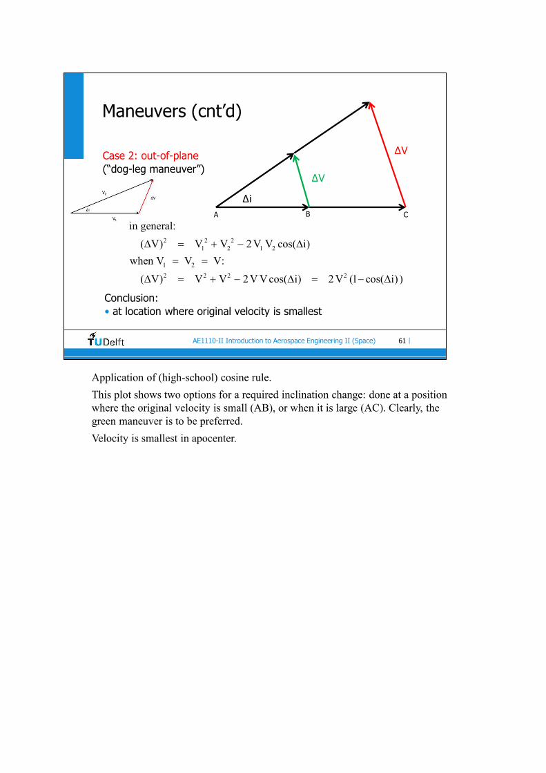
Maneuvers (cnt’d)
Case 2: out-of-plane(“dog-leg maneuver”)
2 2 21 2 1 2
1 2
2 2 2 2
in general:
( V) V V 2 V V cos( i)
when V V V:
( V) V V 2V V cos( i) 2 V (1 cos( i) )
Δi
ΔV
ΔV
A B C
Conclusion:• at location where original velocity is smallest
Application of (high-school) cosine rule.
This plot shows two options for a required inclination change: done at a position where the original velocity is small (AB), or when it is large (AC). Clearly, the green maneuver is to be preferred.
Velocity is smallest in apocenter.

62AE1110-II Introduction to Aerospace Engineering II (Space) |
Maneuvers (cnt’d): example 5
Change inclination of circular parking orbit at 185 km altitude from 28.5° to 0°.
Answer:• velocity in circular parking orbit at 28.5° = √(μ/r) = 7.793 km/s• velocity in circular parking orbit at 0° = 7.793 km/s• ΔV = 2 V sin(Δi/2) = 3.837 km/s
after [Braeunig, 2009]
i
μEarth = 398600.441 km3/s2; REarth = 6378.136 km
The bottom line shows an alternative expression for ΔV for dog-leg maneuvers, which can either be derived from the expression on the previous sheet (remember: cos(α+β) = cos(α) cos(β) – sin(α) sin(β)), or directly observed in a planar triangle: sin(Δi/2) = (ΔV/2)/V.
28.5° is the latitude of Kennedy Space Center (Florida, USA).
63AE1110-II Introduction to Aerospace Engineering II (Space) |
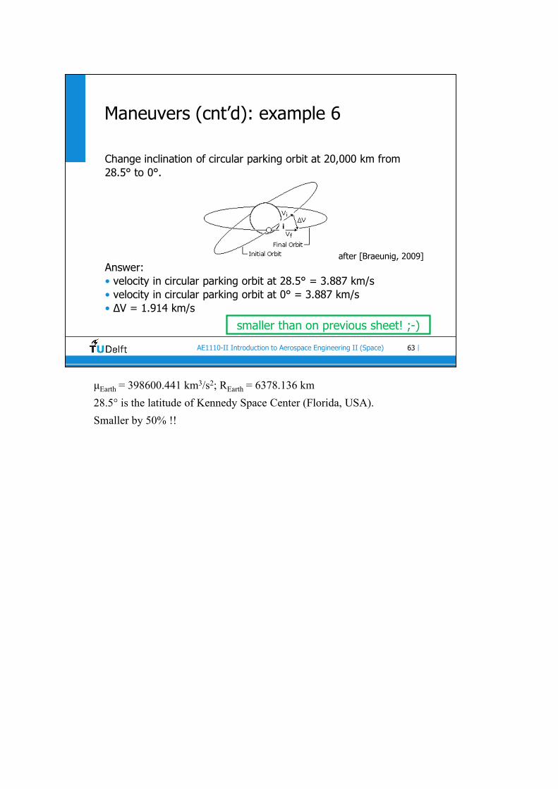
Maneuvers (cnt’d): example 6
Change inclination of circular parking orbit at 20,000 km from 28.5° to 0°.
Answer:• velocity in circular parking orbit at 28.5° = 3.887 km/s• velocity in circular parking orbit at 0° = 3.887 km/s• ΔV = 1.914 km/s
after [Braeunig, 2009]
i
smaller than on previous sheet! ;-)
μEarth = 398600.441 km3/s2; REarth = 6378.136 km
28.5° is the latitude of Kennedy Space Center (Florida, USA).
Smaller by 50% !!
64AE1110-II Introduction to Aerospace Engineering II (Space) |
Maneuvers (cnt’d)
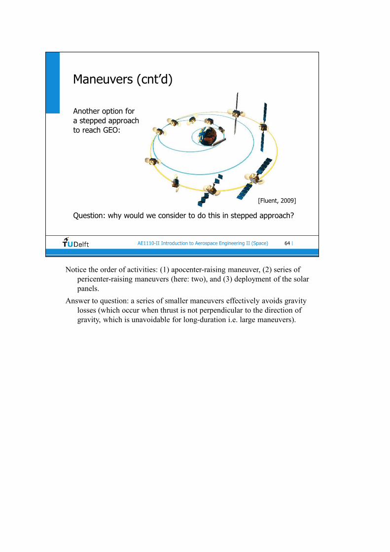
Another option fora stepped approachto reach GEO:
Question: why would we consider to do this in stepped approach?
[Fluent, 2009]
Notice the order of activities: (1) apocenter-raising maneuver, (2) series of pericenter-raising maneuvers (here: two), and (3) deployment of the solar panels.
Answer to question: a series of smaller maneuvers effectively avoids gravity losses (which occur when thrust is not perpendicular to the direction of gravity, which is unavoidable for long-duration i.e. large maneuvers).
65AE1110-II Introduction to Aerospace Engineering II (Space) |
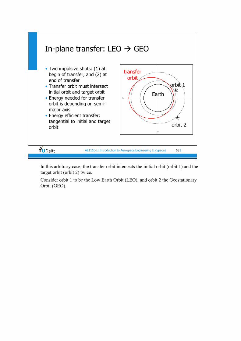
In-plane transfer: LEO GEO
• Two impulsive shots: (1) at begin of transfer, and (2) at end of transfer
• Transfer orbit must intersect initial orbit and target orbit
• Energy needed for transfer orbit is depending on semi-major axis
• Energy efficient transfer: tangential to initial and target orbit
x
y
Earth
orbit 1
transfer orbit
orbit 2
In this arbitrary case, the transfer orbit intersects the initial orbit (orbit 1) and the target orbit (orbit 2) twice.
Consider orbit 1 to be the Low Earth Orbit (LEO), and orbit 2 the Geostationary Orbit (GEO).

66AE1110-II Introduction to Aerospace Engineering II (Space) |
In-plane transfer: LEO GEO (cnt’d)
Solution: Hohmann transfer orbit
• Two impulsive shots: (1) at begin of transfer, and (2) at end of transfer
• Transfer orbit must intersect initial orbit and target orbit
• Energy needed for transfer orbit is depending on semi-major axis
• Energy-efficient transfer: tangential to initial and target orbit
See issue below
67AE1110-II Introduction to Aerospace Engineering II (Space) |
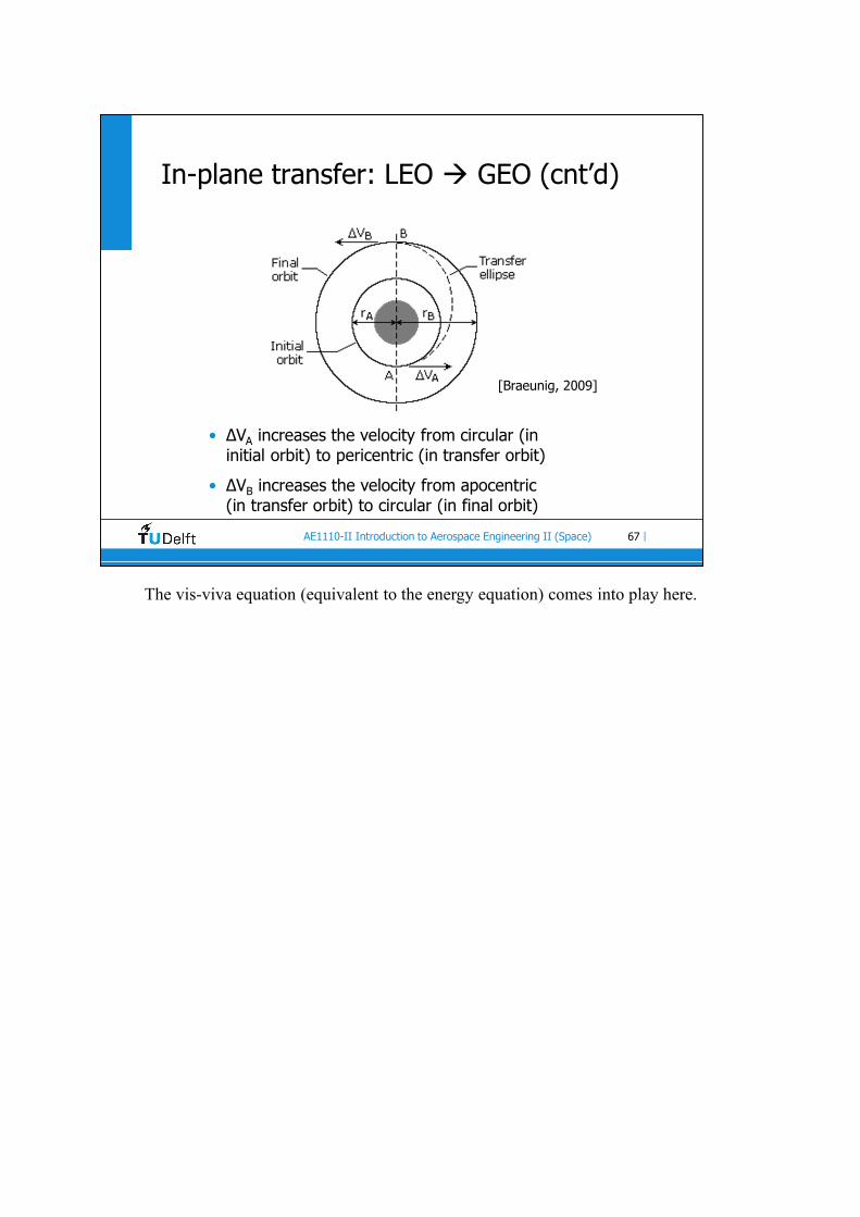
In-plane transfer: LEO GEO (cnt’d)
[Braeunig, 2009]
• ΔVA increases the velocity from circular (in initial orbit) to pericentric (in transfer orbit)
• ΔVB increases the velocity from apocentric (in transfer orbit) to circular (in final orbit)
The vis-viva equation (equivalent to the energy equation) comes into play here.
68AE1110-II Introduction to Aerospace Engineering II (Space) |
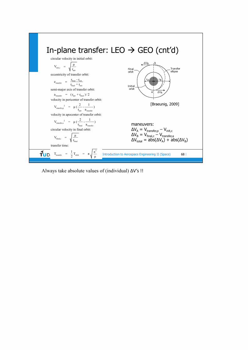
In-plane transfer: LEO GEO (cnt’d)
init,cinit
final inittransfer
final init
transfer init final
circular velocity in initial orbit:
μV
r
eccentricity of transfer orbit:
r - re
r + r
semi-major axis of transfer orbit:
a = ( r + r ) / 2
velocity in pericenter of
2transfer,p
init transfer
2transfer,a
final transfer
final,cfinal
transfer or
transfer orbit:
2 1V = μ ( - )
r a
velocity in apocenter of transfer orbit:
2 1V = μ ( - )
r a
circular velocity in final orbit:
μV =
r
transfer time:
1T = T
2
3
bit
a= π
μ
[Braeunig, 2009]
maneuvers:ΔVA = Vtransfer,p – Vinit,cΔVB = Vfinal,c – Vtransfer,aΔVtotal = abs(ΔVA) + abs(ΔVB)
Always take absolute values of (individual) ΔV’s !!

69AE1110-II Introduction to Aerospace Engineering II (Space) |
In-plane transfer: LEO GEO (cnt’d)
[Braeunig, 2009]
Example: transfer from LEO at 185 km to GEO:
• rinit = 6563.136 km
• rfinal = 42164.173 km
• Vc,init = 7.793 km/s
• Vc,final = 3.075 km/s
• etransfer = 0.7306
• atransfer = 24363.654 km
• Vtransfer,p = 10.252 km/s
• Vtransfer,a = 1.596 km/s
• ΔVA = 2.459 km/s
• ΔVB = 1.479 km/s
• ΔVtotal = 3.938 km/s
• Ttransfer = 18923.202 s = 5 hr 15 min 23.202 s
VERIFY NUMBERS!
μEarth = 398600.441 km3/s2; REarth = 6378.136 km.
Values may be marginally inconsistent because of rounding.

70AE1110-II Introduction to Aerospace Engineering II (Space) |
Maneuvers (cnt’d)
Problem: LEO -> GEO (both circular), with different inclinations
How about the scenario1) change inclination in LEO2) raise apocenter to GEO altitude3) circularize to GEO altitude
good ? bad ?
How about the scenario1) raise apocenter to GEO altitude2) change inclination in apocenter3) circularize to GEO altitude
good ? bad ?
Maneuvers are not only used for transfers between elliptical orbits, but also to escape from Earth!!! (by entering into a hyperbolic orbit)
71AE1110-II Introduction to Aerospace Engineering II (Space) |
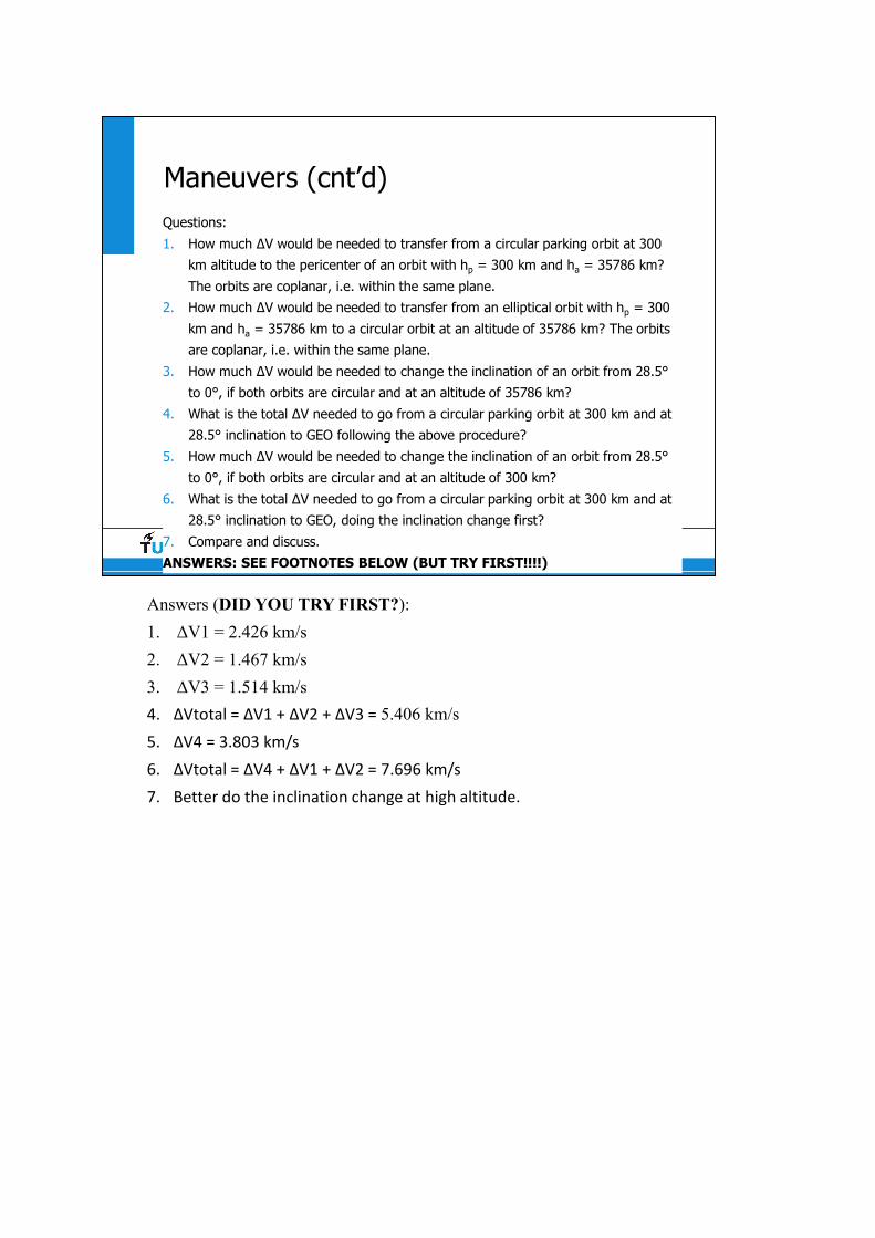
Maneuvers (cnt’d)Questions:
1. How much ΔV would be needed to transfer from a circular parking orbit at 300
km altitude to the pericenter of an orbit with hp = 300 km and ha = 35786 km?
The orbits are coplanar, i.e. within the same plane.
2. How much ΔV would be needed to transfer from an elliptical orbit with hp = 300
km and ha = 35786 km to a circular orbit at an altitude of 35786 km? The orbits
are coplanar, i.e. within the same plane.
3. How much ΔV would be needed to change the inclination of an orbit from 28.5°
to 0°, if both orbits are circular and at an altitude of 35786 km?
4. What is the total ΔV needed to go from a circular parking orbit at 300 km and at
28.5° inclination to GEO following the above procedure?
5. How much ΔV would be needed to change the inclination of an orbit from 28.5°
to 0°, if both orbits are circular and at an altitude of 300 km?
6. What is the total ΔV needed to go from a circular parking orbit at 300 km and at
28.5° inclination to GEO, doing the inclination change first?
7. Compare and discuss.
ANSWERS: SEE FOOTNOTES BELOW (BUT TRY FIRST!!!!)
Answers (DID YOU TRY FIRST?):
1. ΔV1 = 2.426 km/s
2. ΔV2 = 1.467 km/s
3. ΔV3 = 1.514 km/s
4. ΔVtotal = ΔV1 + ΔV2 + ΔV3 = 5.406 km/s
5. ΔV4 = 3.803 km/s
6. ΔVtotal = ΔV4 + ΔV1 + ΔV2 = 7.696 km/s
7. Better do the inclination change at high altitude.
72AE1110-II Introduction to Aerospace Engineering II (Space) |
Maneuvers (cnt’d)
Reality:
• combined maneuvers• gravity losses• fast transfers• low-thrust transfers• …..
see ae2-230-I

73AE1110-II Introduction to Aerospace Engineering II (Space) |
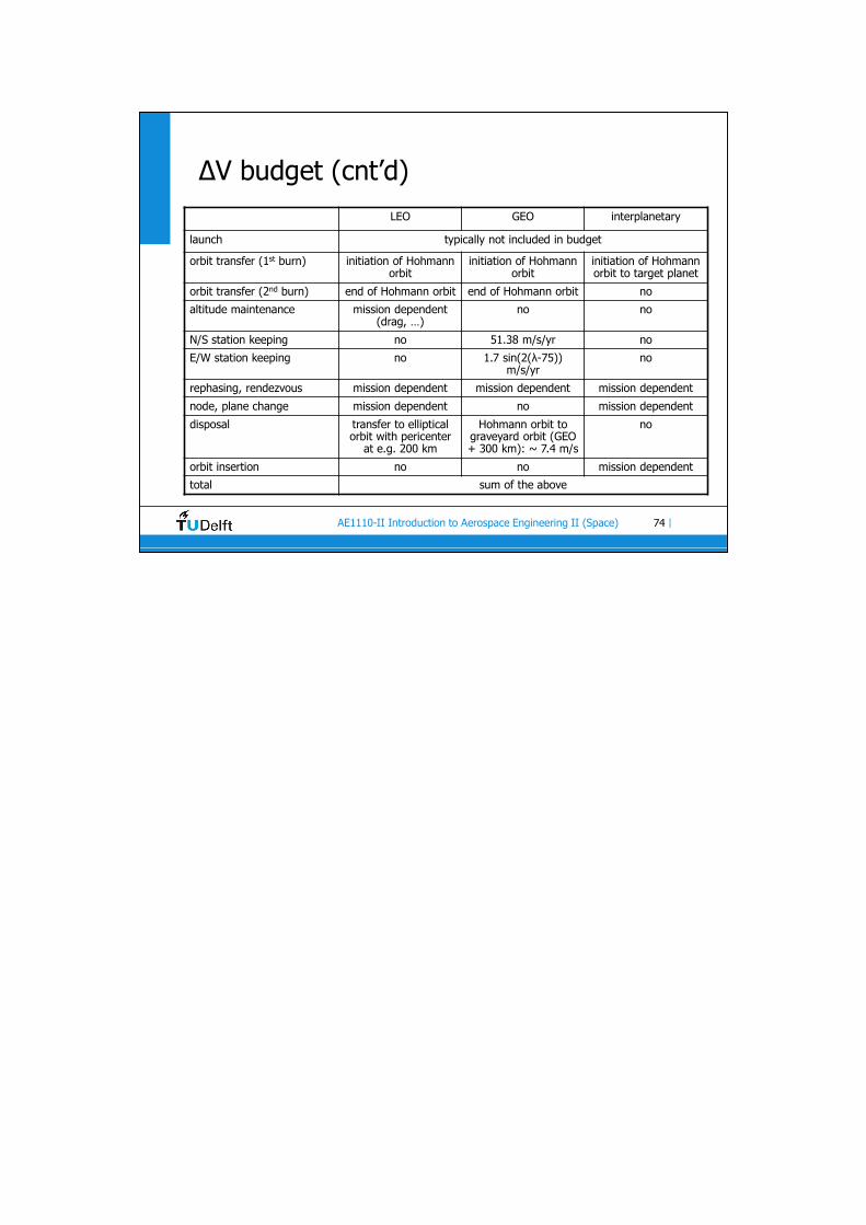
ΔV budget
Why?
• structured way to identify and quantify all maneuvers
• combine all maneuvers in single parameter
• translate to required propellant mass
• evaluate various options mission scenario
74AE1110-II Introduction to Aerospace Engineering II (Space) |
ΔV budget (cnt’d)LEO GEO interplanetary
launch typically not included in budget
orbit transfer (1st burn) initiation of Hohmann orbit
initiation of Hohmann orbit
initiation of Hohmann orbit to target planet
orbit transfer (2nd burn) end of Hohmann orbit end of Hohmann orbit no
altitude maintenance mission dependent (drag, …)
no no
N/S station keeping no 51.38 m/s/yr no
E/W station keeping no 1.7 sin(2(λ-75)) m/s/yr
no
rephasing, rendezvous mission dependent mission dependent mission dependent
node, plane change mission dependent no mission dependent
disposal transfer to elliptical orbit with pericenter
at e.g. 200 km
Hohmann orbit to graveyard orbit (GEO + 300 km): ~ 7.4 m/s
no
orbit insertion no no mission dependent
total sum of the above

Challenge the future
DelftUniversity ofTechnology
Introduction to Aerospace Engineering II (AE1110-II)
Space environmentNovember 26, 2020 (v20.1)
R. Noomen, B.A.C. Ambrosius, J.M. Kuiper, B.T.C. Zandbergen

76AE1110-II Introduction to Aerospace Engineering II (Space) |
Why? Decay of Salyut-7
Not knowing the environment in which a satellite will be operating, can result in a disaster. This example shows the effect of atmospheric drag on the pericenter height of the Russian space station Salyut-7, which was abandoned in 1986 and left to decay in the subsequent years. Source of data: NORAD Two Line Elements.
77AE1110-II Introduction to Aerospace Engineering II (Space) |
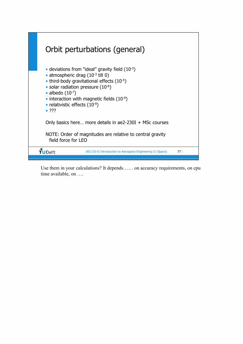
Orbit perturbations (general)
• deviations from “ideal” gravity field (10-3)• atmospheric drag (10-3 till 0) • third-body gravitational effects (10-5)• solar radiation pressure (10-6)• albedo (10-7)• interaction with magnetic fields (10-9)• relativistic effects (10-9)• ???
Only basics here… more details in ae2-230I + MSc courses
NOTE: Order of magnitudes are relative to central gravity field force for LEO
Use them in your calculations? It depends…… on accuracy requirements, on cpu time available, on ….

78AE1110-II Introduction to Aerospace Engineering II (Space) |
Gravity field Earth: theory
sati 2
earth2
G m ρ dvdF =
r
GMr = -
r
Elementary force:
Total acceleration for symmetrical Earth:
satellite: Kepler orbit
Parameter “G” is the universal gravitational constant (6.67259×10⁻¹¹ m3/kg/s2), “msat” represents the mass of the satellite, “r” is the distance between the satellite and a mass element of Earth (first equation) or between the satellite and the center-of-mass of Earth (second equation), “ρ” is the mass density of an element “dv” of Earth [kg/m3], “Mearth” is the total mass of Earth (5.9737×1024 kg). The product of G and Mearth is commonly denoted as “μ” , which is called the gravitational parameter of Earth (=G×Mearth=398600.44×109 m3/s2).

79AE1110-II Introduction to Aerospace Engineering II (Space) |
Gravity field Earth: theory (cnt’d)But:1. real Earth is not perfectly round nor homogeneous2. model for ideal Earth gravity needs corrections3. mathematical description in “spherical harmonics” with
coefficients (scaling factors) Jn,m
4. most important: Earth flattening (J2; relevant for all satellites)5. J2,2 (especially relevant for GEO satellites)
extra mass
The collection of these (and other) terms can be regarded as corrections to the first-order model of a spherical, radially symmetric Earth. The equatorial bulge is represented by the J2 (or J2,0, as depicted in this plot) term, which is the dominant correction term in Earth’s gravity field model. The J-terms are scaling factors.
80AE1110-II Introduction to Aerospace Engineering II (Space) |
Gravity field Earth: theory (cnt’d)
[earthdata.nasa.gov, 2014]
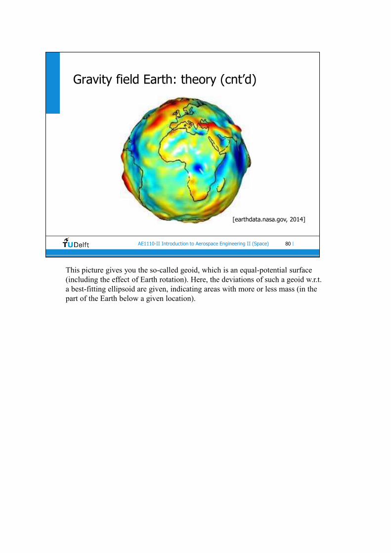
This picture gives you the so-called geoid, which is an equal-potential surface (including the effect of Earth rotation). Here, the deviations of such a geoid w.r.t. a best-fitting ellipsoid are given, indicating areas with more or less mass (in the part of the Earth below a given location).

81AE1110-II Introduction to Aerospace Engineering II (Space) |
Gravity field Earth: satellites (cnt’d)
2
e2π 2 2
RΔΩ = - 3 π J cos(i)
a (1-e )
ad (4): first-order effect on satellite orbits: J2 (flattening or oblateness)
Main consequence:
precession of the ascending node
Change after one orbit:
The net change in Ω, after one complete revolution of the satellite around Earth. J2 is about 1.082×10⁻³. Clearly, it decreases with increasing semi-major axis (subtract earth radius: altitude), and is zero in case the inclination is equal to 90°.
82AE1110-II Introduction to Aerospace Engineering II (Space) |
Gravity field Earth: satellites (cnt’d)
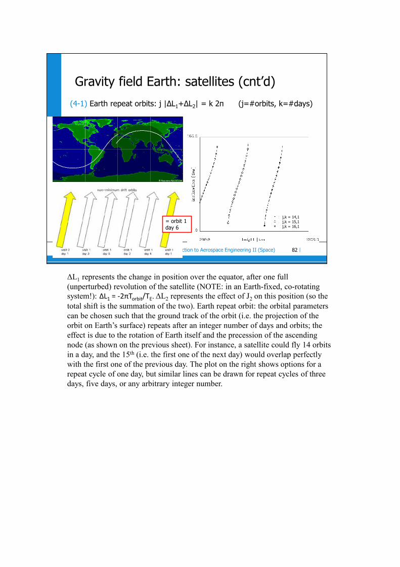
(4-1) Earth repeat orbits: j |ΔL1+ΔL2| = k 2π (j=#orbits, k=#days)
j,k = 14,1j,k = 15,1j,k = 16,1
= orbit 1 day 6
ΔL1 represents the change in position over the equator, after one full (unperturbed) revolution of the satellite (NOTE: in an Earth-fixed, co-rotating system!): ΔL1 = -2πTorbit/TE. ΔL2 represents the effect of J2 on this position (so the total shift is the summation of the two). Earth repeat orbit: the orbital parameters can be chosen such that the ground track of the orbit (i.e. the projection of the orbit on Earth’s surface) repeats after an integer number of days and orbits; the effect is due to the rotation of Earth itself and the precession of the ascending node (as shown on the previous sheet). For instance, a satellite could fly 14 orbits in a day, and the 15th (i.e. the first one of the next day) would overlap perfectly with the first one of the previous day. The plot on the right shows options for a repeat cycle of one day, but similar lines can be drawn for repeat cycles of three days, five days, or any arbitrary integer number.
83AE1110-II Introduction to Aerospace Engineering II (Space) |
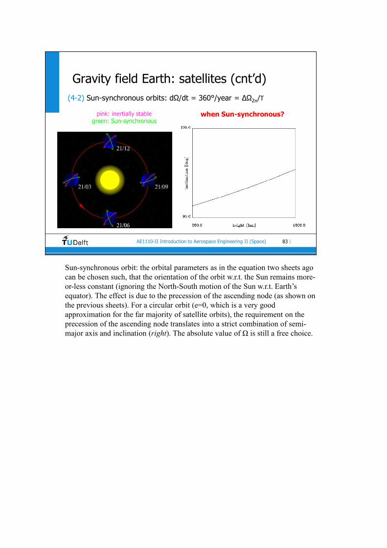
Gravity field Earth: satellites (cnt’d)(4-2) Sun-synchronous orbits: dΩ/dt = 360°/year = ΔΩ2π/T
pink: inertially stablegreen: Sun-synchronous
when Sun-synchronous?
Sun-synchronous orbit: the orbital parameters as in the equation two sheets ago can be chosen such, that the orientation of the orbit w.r.t. the Sun remains more-or-less constant (ignoring the North-South motion of the Sun w.r.t. Earth’s equator). The effect is due to the precession of the ascending node (as shown on the previous sheets). For a circular orbit (e=0, which is a very good approximation for the far majority of satellite orbits), the requirement on the precession of the ascending node translates into a strict combination of semi-major axis and inclination (right). The absolute value of Ω is still a free choice.

84AE1110-II Introduction to Aerospace Engineering II (Space) |
Gravity field Earth: satellites (cnt’d)
ad (5): J2,2 causes an East-West acceleration and drift in GEO[Fortescue & Stark, 1995]:
accEW2,2=-5.6×10⁻⁸ sin(2(λ+14.9)) m/s2
ΔV budget [m/s/yr]:
• J2,2: 1.7 sin(2(λ-75))
• Sun+Moon: 51.4
Although its magnitude is very small, the East-West acceleration on geostationary satellites caused by J2,2 acts continuously in the same direction (the satellite is Earth-fixed!), and hence can build up into a significant effect. This plot gives the acceleration in an Earth-fixed (i.e., co-rotating) system; the effect of the perturbing acceleration is in opposite direction of the acceleration itself. Four equilibrium points can be distinguished. When a satellite is not located in one of these equilibrium points, this acceleration adds to the ΔV budget. The equilibrium points depicted here do not perfectly match the zero-crossings of the equation, since they also include effects of other perturbations from the gravity field.

85AE1110-II Introduction to Aerospace Engineering II (Space) |
Atmosphere: theoryEarth’s atmosphere responds to two types of Solar energy:1. ultra-violet radiation (expressed by the index F10.7)2. highly-energetic particles (expressed by the index Ap)
Solar
Maximum
Solar Minimum
The intensity of ultraviolet radiation (at wavelengths of about 10-7 m) is expressed by the intensity of solar radiation with wavelength 10.7 cm (a so-called “proxy”). The intensity of UV radiation clearly follows the 11-year solar cycle. The number of highly-energetic particles is measured by monitoring their perturbation of Earth’s magnetic field. Their concentration shows a weak correlation with solar activity.
86AE1110-II Introduction to Aerospace Engineering II (Space) |
Atmosphere: theory (cnt’d)
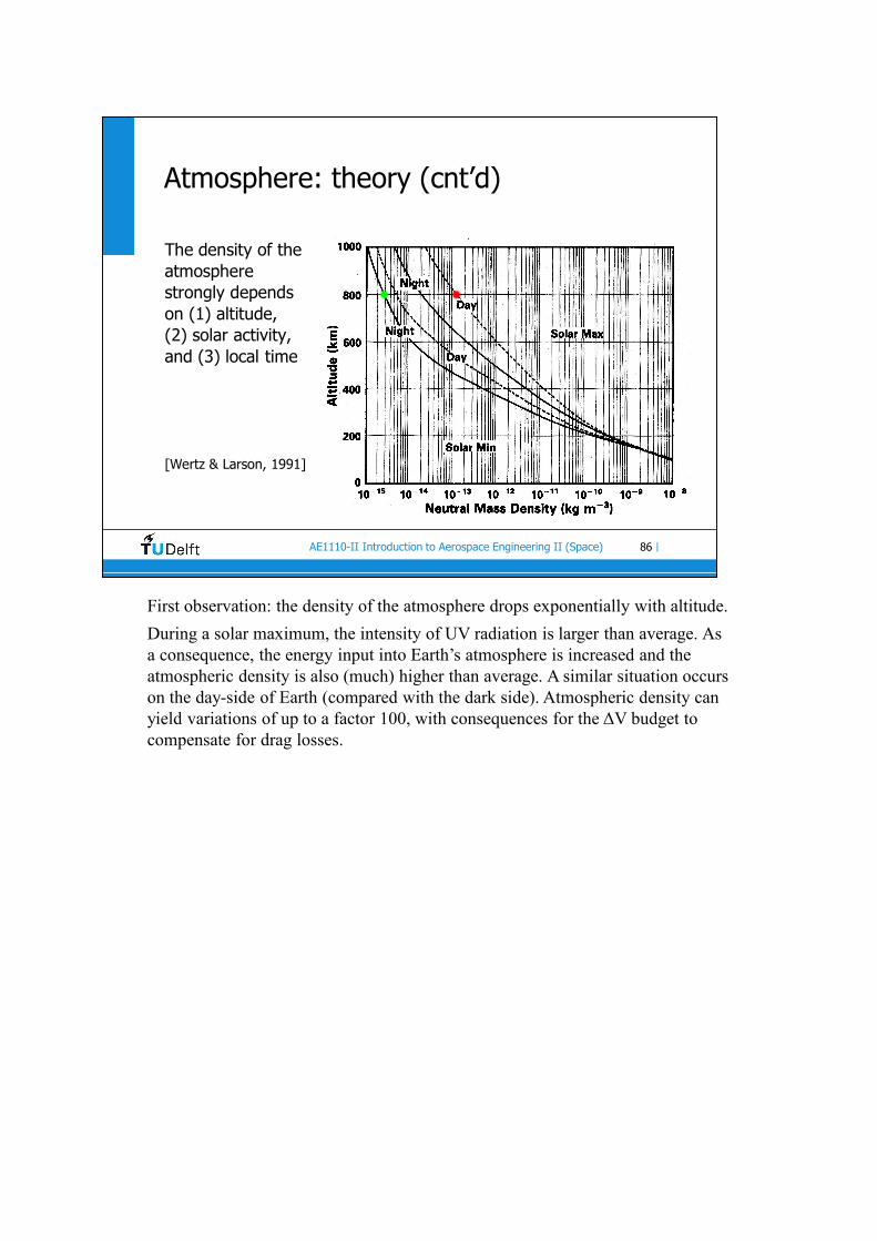
The density of the atmosphere strongly depends on (1) altitude, (2) solar activity, and (3) local time
[Wertz & Larson, 1991]
First observation: the density of the atmosphere drops exponentially with altitude.
During a solar maximum, the intensity of UV radiation is larger than average. As a consequence, the energy input into Earth’s atmosphere is increased and the atmospheric density is also (much) higher than average. A similar situation occurs on the day-side of Earth (compared with the dark side). Atmospheric density can yield variations of up to a factor 100, with consequences for the ΔV budget to compensate for drag losses.
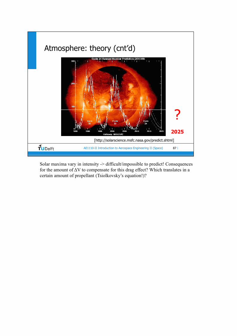
87AE1110-II Introduction to Aerospace Engineering II (Space) |
Atmosphere: theory (cnt’d)
[http://solarscience.msfc.nasa.gov/predict.shtml]
?2025
Solar maxima vary in intensity -> difficult/impossible to predict! Consequences for the amount of ΔV to compensate for this drag effect? Which translates in a certain amount of propellant (Tsiolkovsky’s equation!)?
88AE1110-II Introduction to Aerospace Engineering II (Space) |
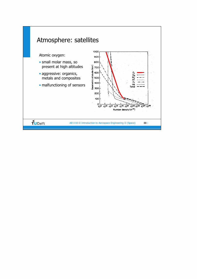
Atmosphere: satellites
Atomic oxygen:
• small molar mass, so present at high altitudes
• aggressive: organics, metals and composites
• malfunctioning of sensors

89AE1110-II Introduction to Aerospace Engineering II (Space) |
Atmosphere: satellites (cnt’d)
2D sat
1a = C ρ V S / M
2
CD = drag coefficient (typical value 2 - 4)
ρ = atmospheric density (uncertainty 15-20%)
V = satellite velocity w.r.t. ambient atmosphere (uncertainty ~1-5%)
S = cross-sectional area satellite (uncertainty ~1%)
CD S / Msat = ballistic coefficient
Acceleration due to atmospheric drag:
The variation of atmospheric density with environmental conditions can be a factor 100 or larger (cf. three sheets earlier); the uncertainty of the models (knowing these environmental conditions) still is 15-20%.
Similar expressions can be written for the lift and side-force components (as well as torques), but the drag acceleration is by far the most important component.

90AE1110-II Introduction to Aerospace Engineering II (Space) |
Atmosphere: satellites (cnt’d)
Consequences atmospheric drag:
1) loss of altitude
2) circularization of orbit
3) limitation of lifetime
common element: loss of energy

91AE1110-II Introduction to Aerospace Engineering II (Space) |
Atmosphere: satellites (cnt’d)ad (1): Behaviour of the pericenter altitude (orbits are nearly circular) of three spacecraft, as a function of time.
The altitude of LAGEOS-1 (top) is such that it is not affected by atmospheric drag. The Russian space station Mir (middle) and the German satellite GFZ-1 (bottom) orbited Earth at about 350 km, where drag is dominant. GFZ-1 is fully passive, but Mir was boosted to a higher orbit once every few months. The orbital decay shows a direct correlation with atmospheric density, which in turn is highly correlated with solar activity. Mir and GFZ-1 are completely different spacecraft, but with more-or-less the same rate of orbital decay.
92AE1110-II Introduction to Aerospace Engineering II (Space) |
Atmosphere: satellites (cnt’d)
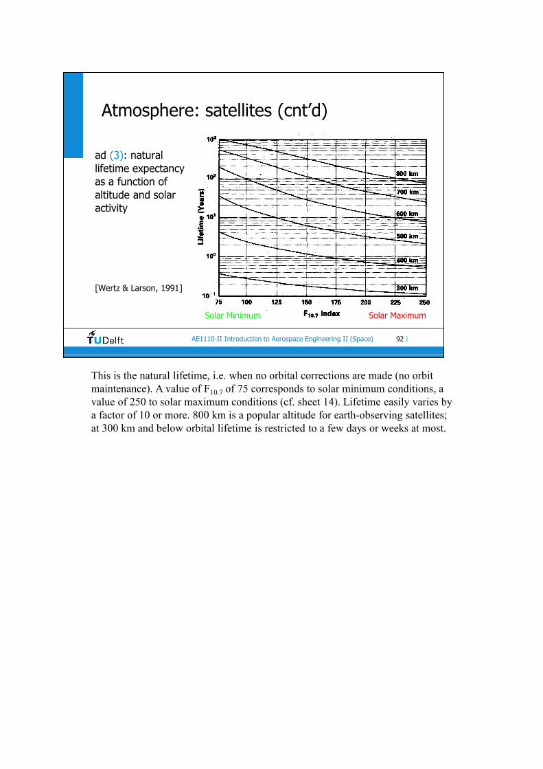
ad (3): natural lifetime expectancy as a function of altitude and solar activity
[Wertz & Larson, 1991]
Solar Minimum Solar Maximum
This is the natural lifetime, i.e. when no orbital corrections are made (no orbit maintenance). A value of F10.7 of 75 corresponds to solar minimum conditions, a value of 250 to solar maximum conditions (cf. sheet 14). Lifetime easily varies by a factor of 10 or more. 800 km is a popular altitude for earth-observing satellites; at 300 km and below orbital lifetime is restricted to a few days or weeks at most.
93AE1110-II Introduction to Aerospace Engineering II (Space) |
Radiation: theory
two types:
• electromagnetic radiation• particle radiation
Electromagnetic radiation: dualistic character: (1) continuous wave, with λ*f=c, and (2) individual photons, each with energy h*f. Source: any object with a temperature different from 0 K. Most prominent for spaceflight: solar radiation, reflected solar radiation (albedo) and thermal radiation from planet(s).
Particle radiation: highly-energetic particles, typically charged. Sources: Sun, other stars, nuclear events, ….

94AE1110-II Introduction to Aerospace Engineering II (Space) |
Radiation: theory (cnt’d)
Illustration of the electromagnetic spectrum [Berkeley Lab, 2001]:
The electromagnetic spectrum shows a huge variation in wavelength, frequency (λ×f=c), and energy (E=h×f). Radiation has a wide variety of sources.
95AE1110-II Introduction to Aerospace Engineering II (Space) |
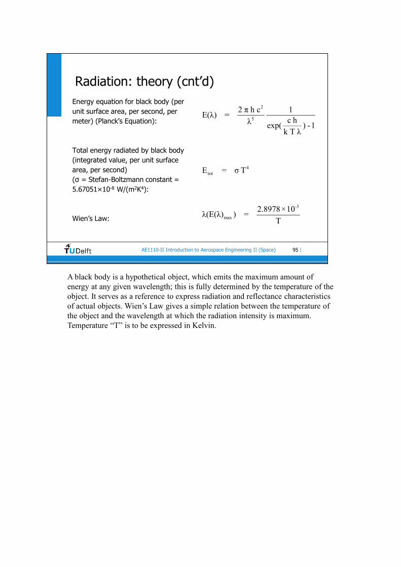
Radiation: theory (cnt’d)Energy equation for black body (per unit surface area, per second, per meter) (Planck’s Equation):
Total energy radiated by black body (integrated value, per unit surface area, per second)(σ = Stefan-Boltzmann constant = 5.67051×10⁻⁸ W/(m2K4):
Wien’s Law:
2
5
4tot
-3
max
2 π h c 1E(λ) =
c hλ exp( ) -1k T λ
E = σ T
2.8978×10λ(E(λ) ) =
T
A black body is a hypothetical object, which emits the maximum amount of energy at any given wavelength; this is fully determined by the temperature of the object. It serves as a reference to express radiation and reflectance characteristics of actual objects. Wien’s Law gives a simple relation between the temperature of the object and the wavelength at which the radiation intensity is maximum. Temperature “T” is to be expressed in Kelvin.
96AE1110-II Introduction to Aerospace Engineering II (Space) |
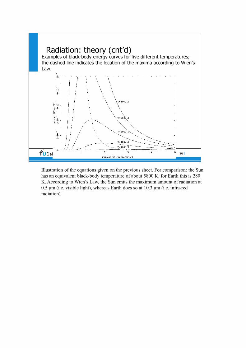
Radiation: theory (cnt’d)Examples of black-body energy curves for five different temperatures; the dashed line indicates the location of the maxima according to Wien’s Law.
Illustration of the equations given on the previous sheet. For comparison: the Sun has an equivalent black-body temperature of about 5800 K, for Earth this is 280 K. According to Wien’s Law, the Sun emits the maximum amount of radiation at 0.5 μm (i.e. visible light), whereas Earth does so at 10.3 μm (i.e. infra-red radiation).

97AE1110-II Introduction to Aerospace Engineering II (Space) |
Radiation: theory (cnt’d)Spacecraft mainly encounter (1) direct solar radiation, (2) albedo radiation and (3) Earth infra-red radiation. Also depicted are two black-body approximations of the latter [Van der Laan, 1986]:
(1)
(2)(3)
The fraction of direct solar radiation reflected by Earth (albedo radiation) depends on wavelength, but a value of about 0.4 can be considered representative for the total effect (left). The infra-red radiation emitted from (not reflected by!) Earth can be approximated by two different black-body curves, which reflect the transparency of Earth’s atmosphere (with two wavelength regions with full transparency, at 8 and 11 μm).
Apologies for the Dutch text!

98AE1110-II Introduction to Aerospace Engineering II (Space) |
Radiation: theory (cnt’d)
Intensity and variability of solar radiation at different wavelength regions [Boettcher, 1991]:
--
total: 1371 ± nothing Solar Constant, SC
Two main messages here:
(1) the majority of solar radiation can be found in the visible spectrum (1000 J/m2.s.μm) (cf. previous two sheets).
(2) The variability in this part of the spectrum is very small, and in regions where variability is large the intensity itself is very small -> total solar radiation intensity is more-or-less constant at a given distance -> the Solar Constant (1371 W/m2) at 1 AU.

99AE1110-II Introduction to Aerospace Engineering II (Space) |
Radiation: satellitesEffects of radiation (electromagnetic and particles) on space missions:1. Attitude control
o Sun sensoro Earth sensoro star sensor
2. Energy supplyo solar panels
3. Thermal control4. Damage
o degradationo thermal effectso electrical damage (Single Event Upsets, SEUs)
5. Orbit perturbations (negative and positive solar sailing)6. Communication7. Astronaut health
[emaze.com, 2015]
[centauri-dreams.org, 2015]
Attitude control: accuracy depends on dimension of target, type of radiation, and requirements.
Energy supply: Si and GaAs cells; efficiencies of up to 30% can be obtained (experimentally).
Thermal control: heat transfer to and from surroundings mostly by radiation (except in (re)entry).
Damage: properties of paint slowly change, structural strength, electrical shorts, …..
Orbit perturbations: solar radiation pressure is one of the dominant forces in GEO satellites.
Communication can be blocked by ionization of the atmosphere.
Astronaut health: nausea, orientation problems, but also increased chances of developing cancer.

100AE1110-II Introduction to Aerospace Engineering II (Space) |
Radiation: satellites (cnt’d)
Ad (2): 2D computation of eclipse length (circular orbit):
e
eclipse
3
eclipse orbit
Earth-central half angle λ: sin λ = R / a
2 λeclipse fraction [%]: T = ×100
360
2 λ 2λ aeclipse length [s]: T = × T = × 2π
360 360 μ
As usual, ”a” represents the semi-major axis and ”Re” Earth’s radius.

101AE1110-II Introduction to Aerospace Engineering II (Space) |
Radiation: satellites (cnt’d)Ad (4): Example of degradation of solar panels, caused by solar particle radiation [Crabb, 1981]:
Degradation:• normally in
LEO: 15% after 4 years
• here: 35% after 3 years
1972
A total reduction of 35% after three years is excessive (but a direct consequence of the chosen orbit: going through the Van Allen Belts every single revolution). The situation is aggrevated by two instantaneous solar flares.
102AE1110-II Introduction to Aerospace Engineering II (Space) |
Radiation: satellites (cnt’d)
Questions:1. Compute, for a satellite in a circular orbit at 300 km altitude,
the eclipse length, both as percentage and in minutes.2. Do the same, for a satellite at 800 km altitude.3. Do the same, for a geostationary satellite.
Answers: see footnotes (BUT TRY FIRST)
Answers (DID YOU TRY? ):
1) Teclipse = 40.4%, or 36.6 min. 2) Teclipse = 34.8%, or 35.1 min. 3) Teclipse = 4.8%, or 69.4 min.

Challenge the future
DelftUniversity ofTechnology
Introduction to Aerospace Engineering II (AE1110-II)
Ground systems and operationsDecember 2, 2020 (v20.1)
R. Noomen, B.A.C. Ambrosius, J.M. Kuiper, B.T.C. Zandbergen
104AE1110-II Introduction to Aerospace Engineering II (Space) |
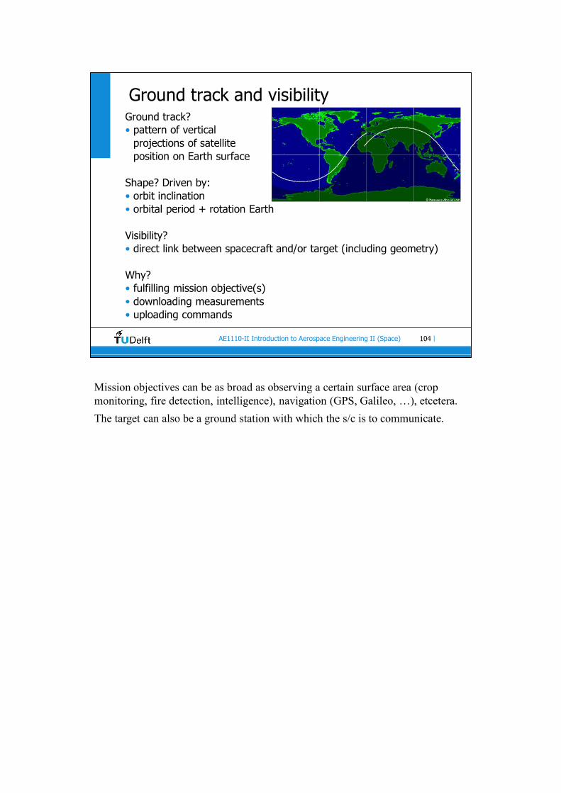
Ground track and visibilityGround track?• pattern of vertical
projections of satelliteposition on Earth surface
Shape? Driven by:• orbit inclination• orbital period + rotation Earth
Visibility?• direct link between spacecraft and/or target (including geometry)
Why?• fulfilling mission objective(s)• downloading measurements• uploading commands
Mission objectives can be as broad as observing a certain surface area (crop monitoring, fire detection, intelligence), navigation (GPS, Galileo, …), etcetera.
The target can also be a ground station with which the s/c is to communicate.
105AE1110-II Introduction to Aerospace Engineering II (Space) |
Ground track and visibility (cnt’d)
Ground track:• the point where the position vector of the satellite crosses
Earth’s surface is called the sub-satellite point• the trace of successive sub-satellite points is the ground
track• during one orbital revolution the ground track typically
describes a sine-like shape• the maximum latitude is equal to the inclination
(or 180° – i)• the ground track is shifted westward by
ΔΛ=15×T (ΔΛ in deg, T is orbital period in hrs)• LEO: ΔΛ~23°• direct contact possible when the satellite is within the
visibility circle around a station/target• size of visibility circle depends on satellite altitude and
minimum elevation
106AE1110-II Introduction to Aerospace Engineering II (Space) |
Ground track and visibility (cnt’d)
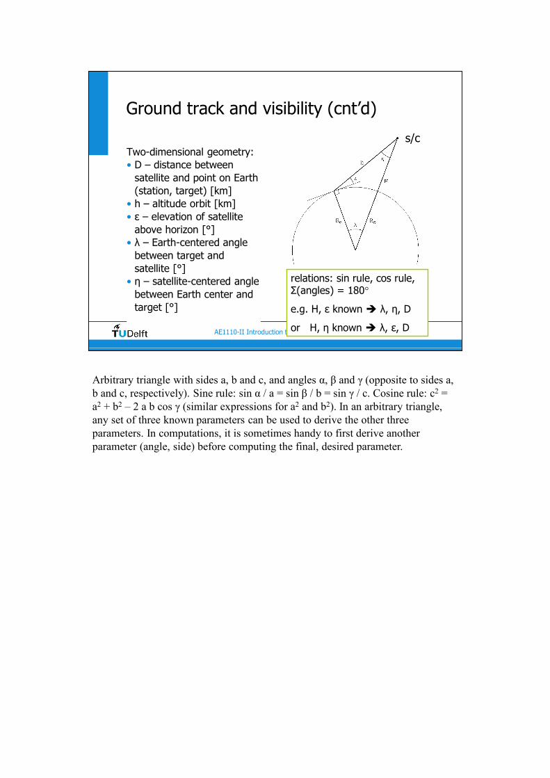
Two-dimensional geometry:• D – distance between
satellite and point on Earth (station, target) [km]
• h – altitude orbit [km]• ε – elevation of satellite
above horizon [°]• λ – Earth-centered angle
between target and satellite [°]
• η – satellite-centered angle between Earth center and target [°]
relations: sin rule, cos rule, Σ(angles) = 180°
e.g. H, ε known λ, η, D
or H, η known λ, ε, D
s/c
Arbitrary triangle with sides a, b and c, and angles α, β and γ (opposite to sides a, b and c, respectively). Sine rule: sin α / a = sin β / b = sin γ / c. Cosine rule: c2 = a2 + b2 – 2 a b cos γ (similar expressions for a2 and b2). In an arbitrary triangle, any set of three known parameters can be used to derive the other three parameters. In computations, it is sometimes handy to first derive another parameter (angle, side) before computing the final, desired parameter.

107AE1110-II Introduction to Aerospace Engineering II (Space) |
Ground track and visibility (cnt’d): example 1
Consider Envisat (h = 780 km, minimum ground elevation 20°)
• question: what is the maximum distance D?
• solution:
e e
e
sin (90+ε) sin η= η = 56.86°
R +H R
(90+ε) + λ + η = 180 λ = 13.14°
sin λ sin(90+ε)= D = 1732.2 km
D R +H
Re = 6378.136 km
108AE1110-II Introduction to Aerospace Engineering II (Space) |
Ground track and visibility (cnt’d): example 2
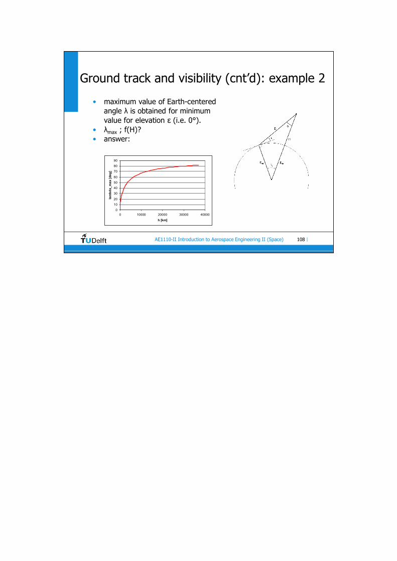
• maximum value of Earth-centered angle λ is obtained for minimum value for elevation ε (i.e. 0°).
• λmax ; f(H)?• answer:
0
10
20
30
40
50
60
70
80
90
0 10000 20000 30000 40000
h [km]
lam
bd
a_m
ax
[d
eg
]
109AE1110-II Introduction to Aerospace Engineering II (Space) |
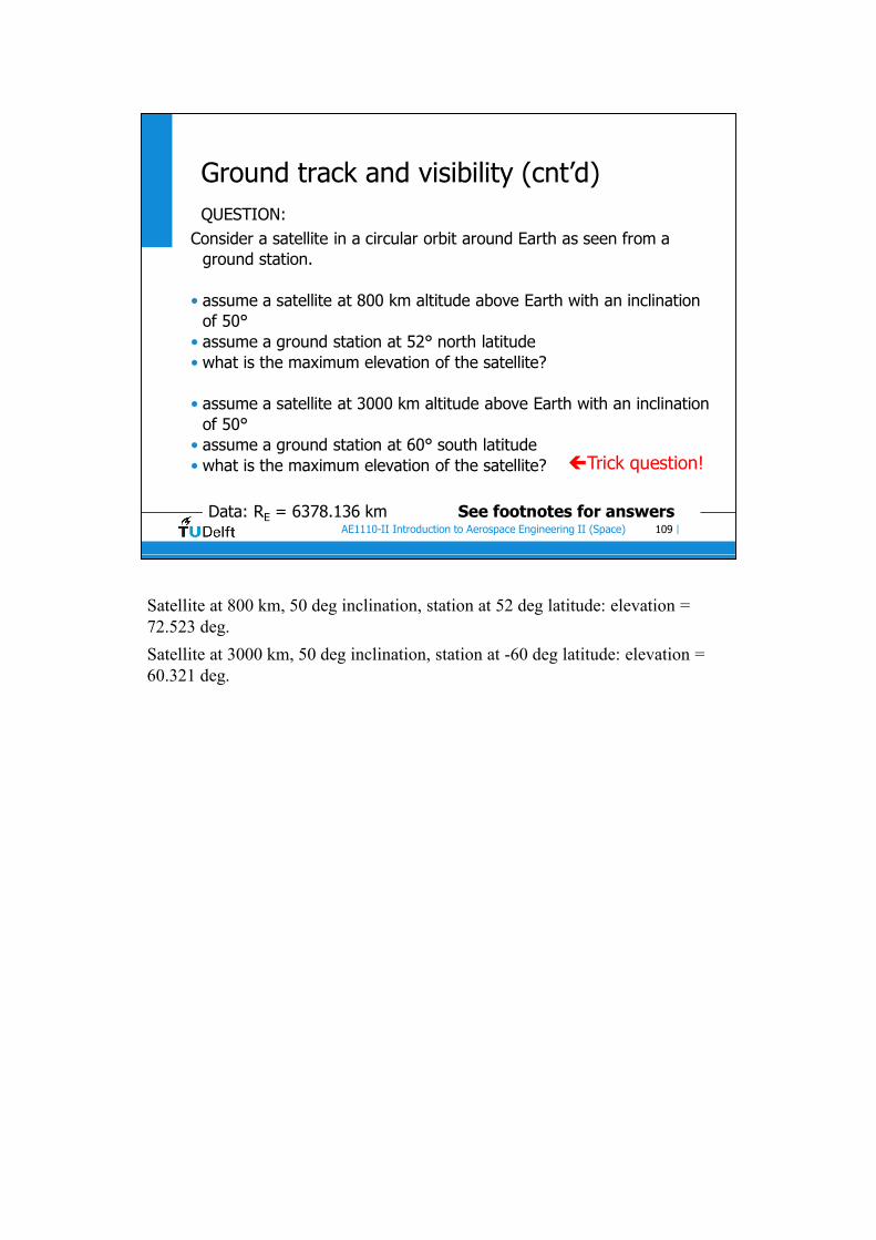
Consider a satellite in a circular orbit around Earth as seen from a ground station.
• assume a satellite at 800 km altitude above Earth with an inclination of 50°
• assume a ground station at 52° north latitude• what is the maximum elevation of the satellite?
• assume a satellite at 3000 km altitude above Earth with an inclination of 50°
• assume a ground station at 60° south latitude• what is the maximum elevation of the satellite?
Ground track and visibility (cnt’d)
Data: RE = 6378.136 km
QUESTION:
See footnotes for answers
Trick question!
Satellite at 800 km, 50 deg inclination, station at 52 deg latitude: elevation = 72.523 deg.
Satellite at 3000 km, 50 deg inclination, station at -60 deg latitude: elevation = 60.321 deg.

110AE1110-II Introduction to Aerospace Engineering II (Space) |
Consider a satellite in a circular orbit around Earth as seen from a ground station.
• assume a satellite at 3000 km altitude above Earth with inclination = 50°
• assume a ground station at 40° north latitude• what is the maximum elevation of the satellite?
Ground track and visibility (cnt’d)
Data: RE = 6378.136 km
QUESTION:
Trick question!
90 degrees (i.e. the satellite is at zenith).
111AE1110-II Introduction to Aerospace Engineering II (Space) |
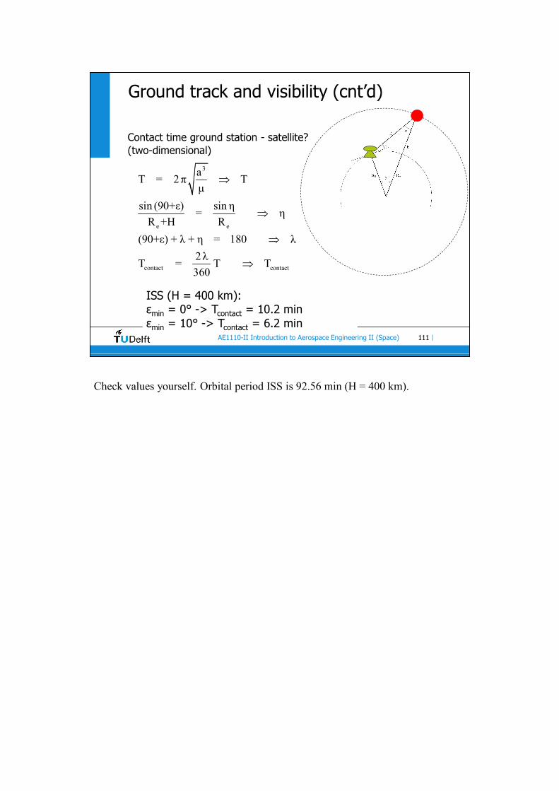
Contact time ground station - satellite?(two-dimensional)
Ground track and visibility (cnt’d)
3
e e
contact contact
aT = 2 π T
μ
sin (90+ε) sin η= η
R +H R
(90+ε) + λ + η = 180 λ
2 λT = T T
360
ISS (H = 400 km):εmin = 0° -> Tcontact = 10.2 minεmin = 10° -> Tcontact = 6.2 min
Check values yourself. Orbital period ISS is 92.56 min (H = 400 km).
112AE1110-II Introduction to Aerospace Engineering II (Space) |
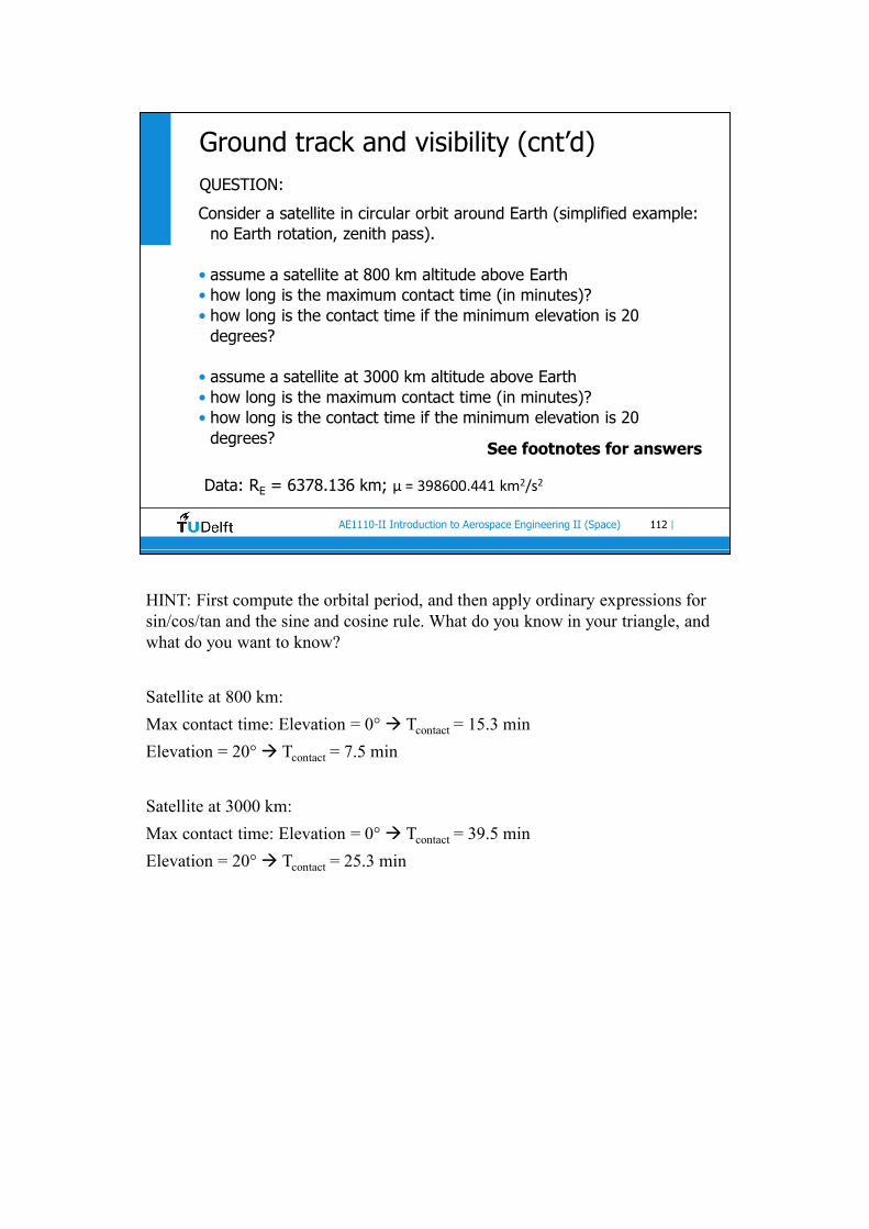
Consider a satellite in circular orbit around Earth (simplified example: no Earth rotation, zenith pass).
• assume a satellite at 800 km altitude above Earth• how long is the maximum contact time (in minutes)?• how long is the contact time if the minimum elevation is 20
degrees?
• assume a satellite at 3000 km altitude above Earth• how long is the maximum contact time (in minutes)?• how long is the contact time if the minimum elevation is 20
degrees?
Ground track and visibility (cnt’d)
Data: RE = 6378.136 km; μ = 398600.441 km2/s2
QUESTION:
See footnotes for answers
HINT: First compute the orbital period, and then apply ordinary expressions for sin/cos/tan and the sine and cosine rule. What do you know in your triangle, and what do you want to know?
Satellite at 800 km:
Max contact time: Elevation = 0° Tcontact = 15.3 min
Elevation = 20° Tcontact = 7.5 min
Satellite at 3000 km:
Max contact time: Elevation = 0° Tcontact = 39.5 min
Elevation = 20° Tcontact = 25.3 min
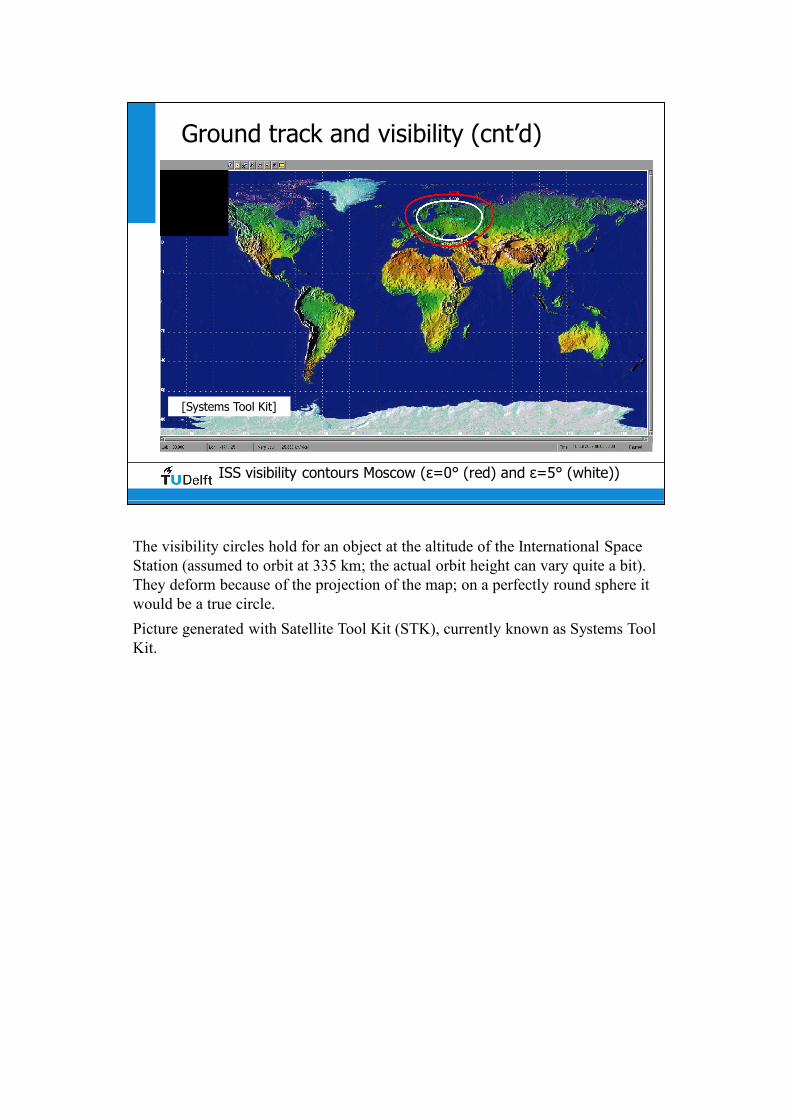
113AE1110-II Introduction to Aerospace Engineering II (Space) |
Ground track and visibility (cnt’d)
ISS visibility contours Moscow (ε=0° (red) and ε=5° (white))
[Systems Tool Kit]
The visibility circles hold for an object at the altitude of the International Space Station (assumed to orbit at 335 km; the actual orbit height can vary quite a bit). They deform because of the projection of the map; on a perfectly round sphere it would be a true circle.
Picture generated with Satellite Tool Kit (STK), currently known as Systems Tool Kit.

114AE1110-II Introduction to Aerospace Engineering II (Space) |
Ground track and visibility (cnt’d)
Ground track ISS on July 10, 2009 (00.00 hrs – 04.00 hrs UTC)
[Systems Tool Kit]
The ISS moves from west (left) to East (right) (orbit inclination is about 52 degrees), but successive ground tracks shift to the West. The simulation covers about 2.5 orbital revolutions. Picture generated with Satellite Tool Kit (STK), currently known as Systems Tool Kit. The visibility contours around Moscow look elongated in East-West direction, which is a mere consequence of the Mercator projection.
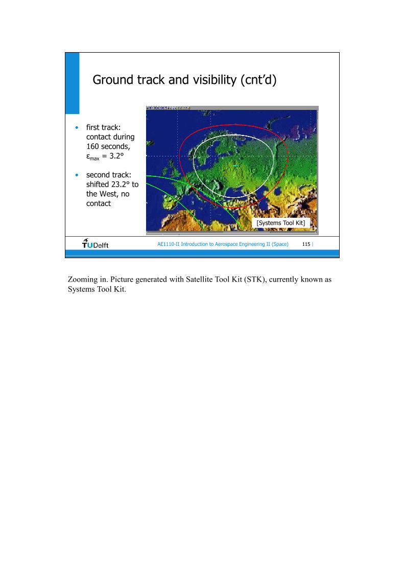
115AE1110-II Introduction to Aerospace Engineering II (Space) |
Ground track and visibility (cnt’d)
• first track: contact during 160 seconds, εmax = 3.2°
• second track: shifted 23.2° to the West, no contact
[Systems Tool Kit]
Zooming in. Picture generated with Satellite Tool Kit (STK), currently known as Systems Tool Kit.

116AE1110-II Introduction to Aerospace Engineering II (Space) |
Communication (cnt’d)Earth coverage: GEO (Intelsat, left) vs. LEO (Globalstar and Iridium, right):
[Systems Tool Kit]
Picture generated with Satellite Tool Kit (STK). The LEO satellites Globalstar and Iridium are not necessarily located above the equator. The coverage area of a single spacecraft at a particular altitude has consequences for the required number of satellites to provide continuous and full global coverage… Starlink!
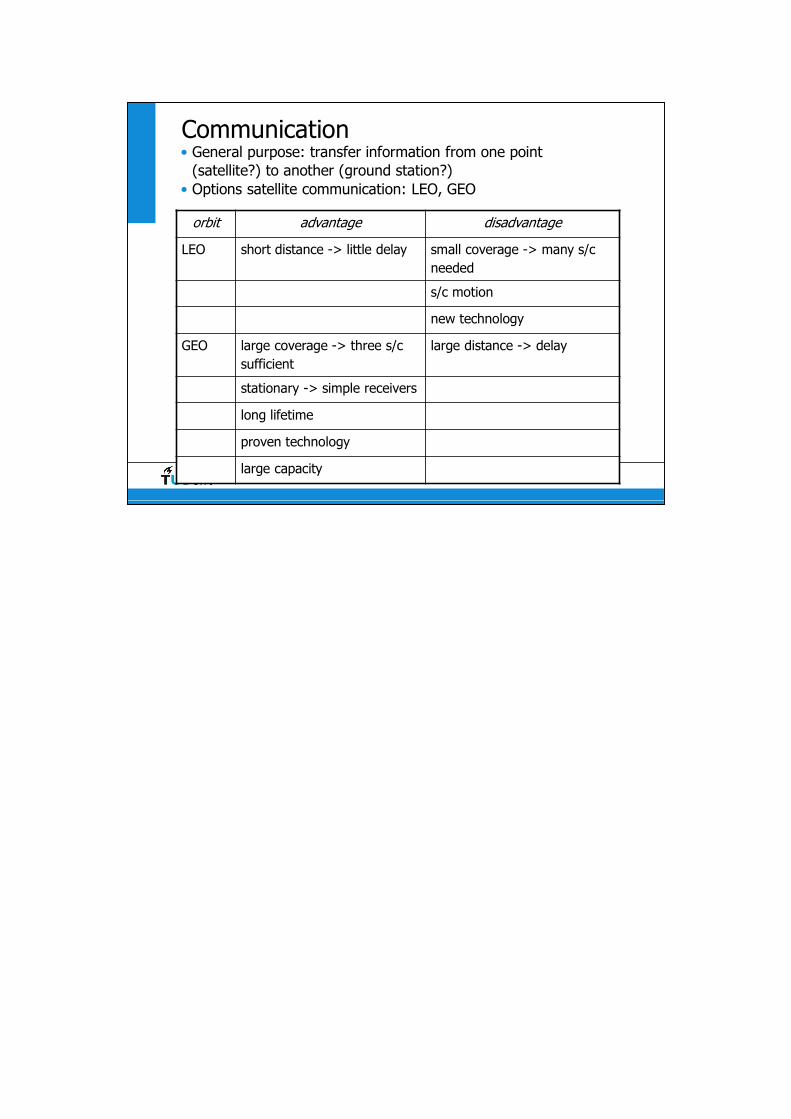
117AE1110-II Introduction to Aerospace Engineering II (Space) |
Communication• General purpose: transfer information from one point
(satellite?) to another (ground station?)• Options satellite communication: LEO, GEO
orbit advantage disadvantage
LEO short distance -> little delay small coverage -> many s/c needed
s/c motion
new technology
GEO large coverage -> three s/c sufficient
large distance -> delay
stationary -> simple receivers
long lifetime
proven technology
large capacity

118AE1110-II Introduction to Aerospace Engineering II (Space) |
Communication (cnt’d)type two-way trip
time [msec]capacity cost [M$]
spacecraft (radio):
LEO 10 * up to 8 Mbit/s [4] 2900 [5]
GEO 267 Gbit/s
submarine cables:
Hibernia Atlantic(transatlantic)
< 70 up to 10.16 Tbit/s [2]
transatlantic(ZBLAN fibers)
59 [1] 300
transarctic 170 [3] Tbit/s [3] 600-1500 [3]
spacecraft (optical)
LGS Innovations Gbit/s – Tbit/s [6]
European DataRelay System
1.8 Gbit/s [7]
*: using one s/c
Round-trip delay time using spacecraft: O(40,000) km divided by speed of light = 267 millisec (GEO); O(1500) km divided by speed of light = 10 millisec (LEO) (not counting internal delays at s/c).
Ref [1]: http://www.telegraph.co.uk/technology/news/875378/The-300m-cable-that-will-save-traders-milliseconds.html
Ref [2]: https://en.wikipedia.org/wiki/Transatlantic-communications-cable
Ref [3]: http://www.extremetech.com/extreme/122989-1-5-billion-the-cost-of-cutting-london-to-tokyo-latency-by-60ms
Ref [4]: Iridium NEXT; argo.ucsd.edu
Ref [5]: http://space.skyrocket.de/doc_sdat/iridium-next.htm
Ref [6]: Aviation Week & Space Technology, August 1-14, 2016, pp. 56-57
Ref [7]: https://en.wikipedia.org/wiki/European_Data_Relay_System
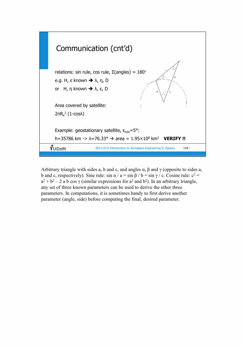
119AE1110-II Introduction to Aerospace Engineering II (Space) |
Communication (cnt’d)
relations: sin rule, cos rule, Σ(angles) = 180°
e.g. H, ε known λ, η, D
or H, η known λ, ε, D
Area covered by satellite:
2πRe2 (1-cosλ)
Example: geostationary satellite, εmin=5°:
h=35786 km -> λ=76.33° area = 1.95×10⁸ km2 VERIFY !!
Arbitrary triangle with sides a, b and c, and angles α, β and γ (opposite to sides a, b and c, respectively). Sine rule: sin α / a = sin β / b = sin γ / c. Cosine rule: c2 = a2 + b2 – 2 a b cos γ (similar expressions for a2 and b2). In an arbitrary triangle, any set of three known parameters can be used to derive the other three parameters. In computations, it is sometimes handy to first derive another parameter (angle, side) before computing the final, desired parameter.

120AE1110-II Introduction to Aerospace Engineering II (Space) |
Communication (cnt’d)Earth coverage of GEO satellites:
• geosynchronous satellite proposed by Herman Noordung (1928)• communication system proposed by Arthur C. Clarke (1945)
• stationary, so contact or not• three satellites can cover full Earth
0
10
20
30
40
50
60
70
80
90
0 10000 20000 30000 40000
h [km]
lam
bd
a_m
ax [
deg
]
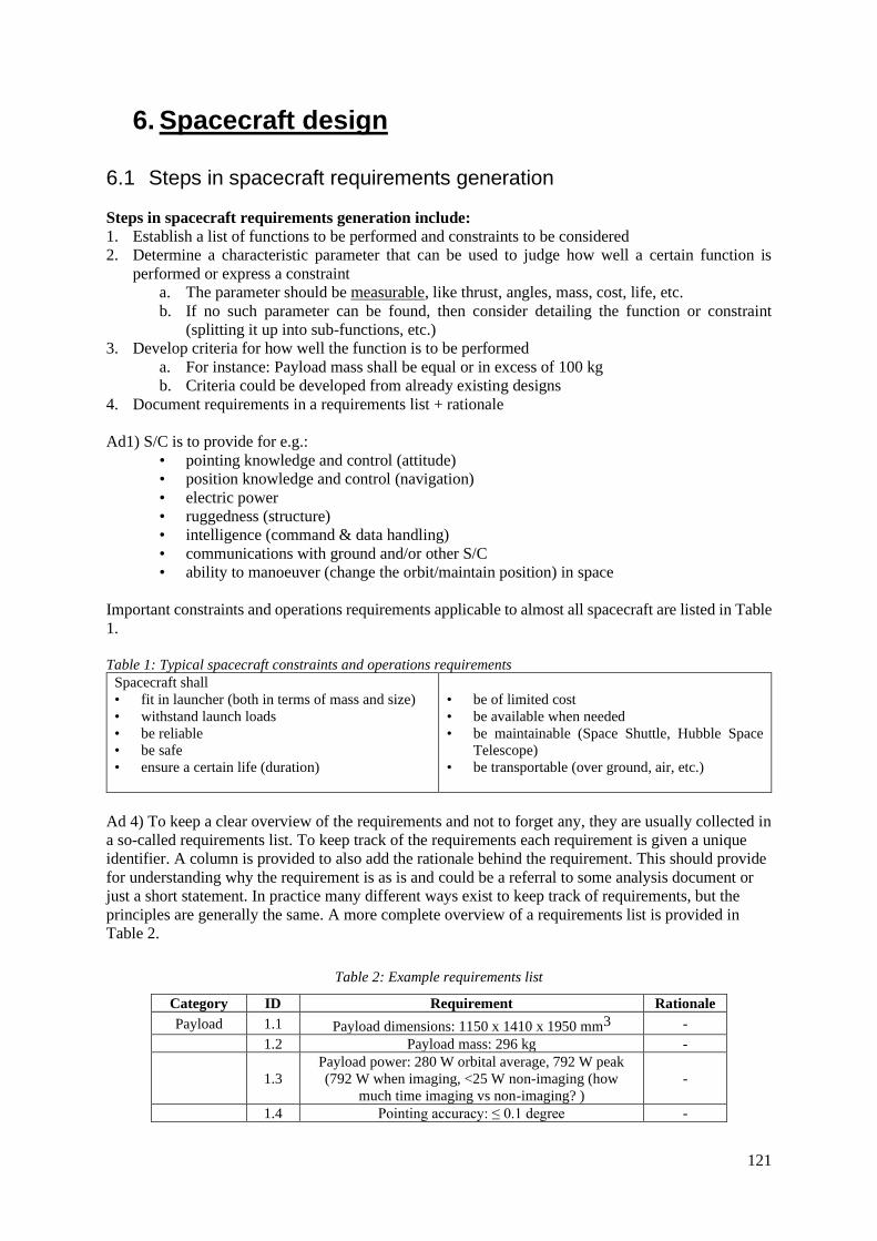
121
6. Spacecraft design 6.1 Steps in spacecraft requirements generation
Steps in spacecraft requirements generation include:
1. Establish a list of functions to be performed and constraints to be considered
2. Determine a characteristic parameter that can be used to judge how well a certain function is
performed or express a constraint
a. The parameter should be measurable, like thrust, angles, mass, cost, life, etc.
b. If no such parameter can be found, then consider detailing the function or constraint
(splitting it up into sub-functions, etc.)
3. Develop criteria for how well the function is to be performed
a. For instance: Payload mass shall be equal or in excess of 100 kg
b. Criteria could be developed from already existing designs
4. Document requirements in a requirements list + rationale
Ad1) S/C is to provide for e.g.:
• pointing knowledge and control (attitude)
• position knowledge and control (navigation)
• electric power
• ruggedness (structure)
• intelligence (command & data handling)
• communications with ground and/or other S/C
• ability to manoeuver (change the orbit/maintain position) in space
Important constraints and operations requirements applicable to almost all spacecraft are listed in Table
1.
Table 1: Typical spacecraft constraints and operations requirements
Spacecraft shall
• fit in launcher (both in terms of mass and size)
• withstand launch loads
• be reliable
• be safe
• ensure a certain life (duration)
• be of limited cost
• be available when needed
• be maintainable (Space Shuttle, Hubble Space
Telescope)
• be transportable (over ground, air, etc.)
Ad 4) To keep a clear overview of the requirements and not to forget any, they are usually collected in
a so-called requirements list. To keep track of the requirements each requirement is given a unique
identifier. A column is provided to also add the rationale behind the requirement. This should provide
for understanding why the requirement is as is and could be a referral to some analysis document or
just a short statement. In practice many different ways exist to keep track of requirements, but the
principles are generally the same. A more complete overview of a requirements list is provided in
Table 2.
Table 2: Example requirements list
Category ID Requirement Rationale
Payload 1.1 Payload dimensions: 1150 x 1410 x 1950 mm3 -
1.2 Payload mass: 296 kg -
1.3
Payload power: 280 W orbital average, 792 W peak
(792 W when imaging, <25 W non-imaging (how
much time imaging vs non-imaging? )
-
1.4 Pointing accuracy: ≤ 0.1 degree -

122
1.5 Pointing stability (drift): ≤ 0.01 degree/s -
1.6 Pointing knowledge: ≤ 0.001 degree -
1.7 Temperature range: -10 deg C - + 30 deg C -
1.8 Transmission capability: ≥ 320 Mbps -
Orbit 2.1 Target: LEO (polar) -
2.2 Drag compensation v ≥ 700 m/s -
Launcher 3.1 Launch mass: ≤ 1200 kg -
3.2 Launcher payload envelope: 4000 mm x 1500 mm (D) -
3.3 Direct launch in polar orbit -
Other 4.1 Reliability: ≥ 0.9 (to ensure reliability of S/C including
payload better than 0.8) -
4.2 Cost: ≤ 80 M$ (FY 2000) -
4.3 Lifetime: ≥ 5 yr in orbit (+ 2 yrs in ground storage) -
4.4 Series size (number of S/C): 40 -
Note that in the table the space system element is identified where the requirement originated from next
to a category of “other requirements” that are related to programmatic issues, operations, or still other.
An example requirements document can be obtained from: Three Corner Sat, 2008, retrieved 27-01-
2015, from http://spacegrant.colorado.edu/COSGC_Projects/Past_Projects/3cs/software/srs.html.
This example may be a little bit overwhelming as it shows many requirements. For now though it
suffices to say that we do not expect you to be able to generate such a document at this stage of your
study, but that you at least should understand the idea behind requirements generation, know about
some definitions and that you have an initial capability of developing spacecraft requirements from
scratch and that you know about the requirements (SMART) on requirements, see later entry, and a
basic ability to do so.
Requirements flow down
Some spacecraft requirements flow down from the program objectives and constraints. Typically a
space program shall be conducted within a certain time frame and at a certain cost. As all elements
constituting the space mission bear costs, it should be determined early on the budget available for the
spacecraft and in more detail the platform. Hence this will lead to requirements flowing down the
spacecraft to the spacecraft subsystems, their components and so on. Hence, once the spacecraft
requirements are know we can start its design. From the design requirements will be derived for the
subsystems and so on (requirements flow down).

123
6.2 Requirements on requirements generation
Defining requirements can be a lengthy process, but ill-defined requirements can be very detrimental
for a space project.
For instance, a requirement like that the spacecraft shall never fail is not considered a good requirement
as this will become a very expensive requirement. For a requirement to be a good requirement, it needs
to be defined in a “SMART” way. The meaning of the acronym SMART in this sense is:
• Specific – Requirements should specify what they are to achieve.
• Measurable – The requirements should provide a metric whereby all stakeholders can determine if
the objectives are being met.
• Achievable or Attainable – Are the requirements’ objectives achievable and attainable, i.e. is it
possible physically for the system to exhibit that requirement under the given conditions. Some
requirements may be beyond the bounds of human knowledge. Others may have theoretical
solutions but be beyond what is currently achievable, like:
− "The system shall be 100% reliable".
− "The system shall be 100% available".
− "The system shall have a minimum response to a query of 1 second irrespective of system load".
To determine whether a requirement is attainable, it is good to ask oneself whether it has been done
before (e.g. in past missions) and if not, why not?
• Realistic – Are the requirements realistic with respect to available resources?
To determine whether a requirement is realisable or not is the most difficult part of creating a
SMART requirement. It is definitely linked with a requirement being attainable or not and one may
say that if it is not attainable, than it is definitely not realisable. Still, if it is attainable, it does not
necessarily be realisable. To determine whether an attainable requirement is realisable, we should
ask ourselves whether this requirement can be satisfied given:
− other system and physical constraints that we have?
− project resource (funding, schedule, availability, etc.) constraints which we must work to?
For example, if there is a requirement to have 99% reliability but the project budget does not permit
the inclusion of the extensive reliability measures needed to satisfy that requirement then that
requirement is not realistic. To decide whether a requirement is realistic sometimes extensive
analyses are needed.
• Time-bound or Traceable – Time-bound refers to when the requirements’ objectives are to be
realized? Time-bound may also be replaced by traceable, meaning that requirements on a lower
level (more detailed design) depend on requirements on a higher level. As an example, we mention
S/C-cost, -reliability, and -life (lower level), which depend on requirements concerning mission
cost, mission reliability and mission life (higher level). Traceability requires that a system is in
place that helps to find out to which higher level requirement a lower level requirement relates. For
instance, this could be a numbering system where the higher level requirements are given a number
X and the lower level requirements a number X.Y, where X denotes the higher level requirement
and Y is a counter that tells how many lower level requirements are derived from this one higher
level requirement.
Generally speaking, if one on the above criteria is not met, we do not have a properly defined
requirement.
To help you in your understanding of the above, the next table lists words that are considered forbidden
to be included in proper requirements. The words have been taken from a presentation by ESA on
requirements generation.
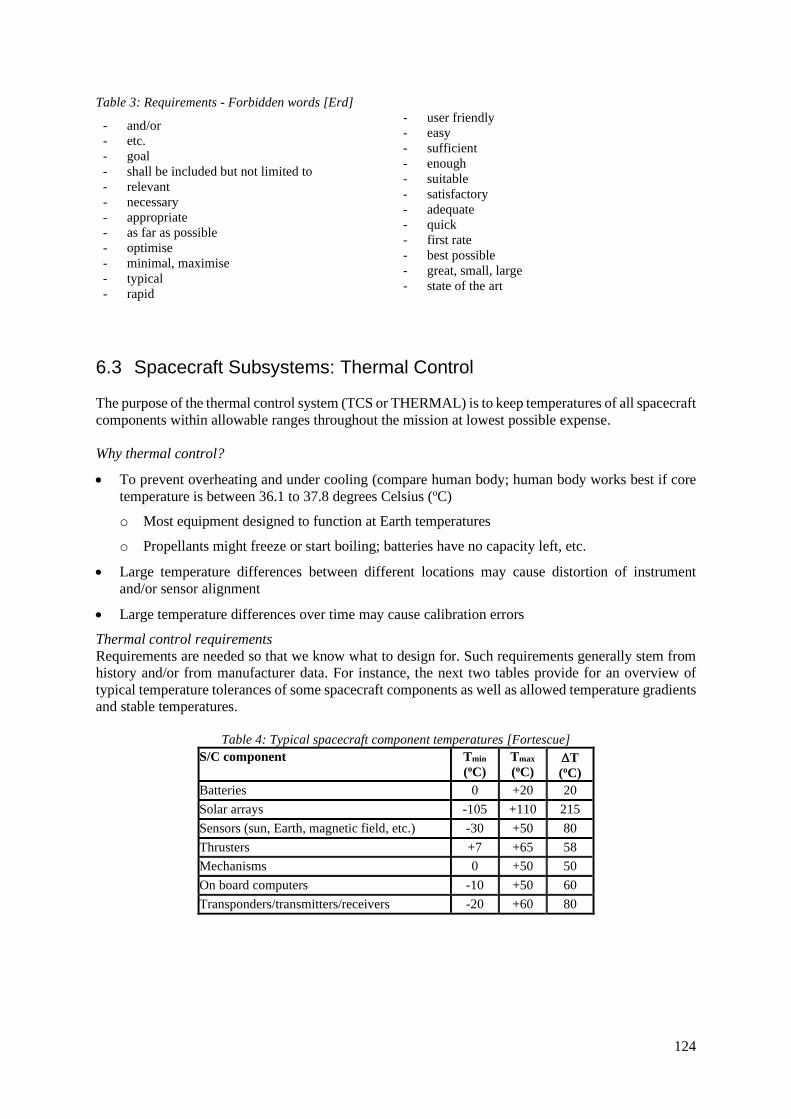
124
Table 3: Requirements - Forbidden words [Erd]
- and/or
- etc.
- goal
- shall be included but not limited to
- relevant
- necessary
- appropriate
- as far as possible
- optimise
- minimal, maximise
- typical
- rapid
- user friendly
- easy
- sufficient
- enough
- suitable
- satisfactory
- adequate
- quick
- first rate
- best possible
- great, small, large
- state of the art
6.3 Spacecraft Subsystems: Thermal Control
The purpose of the thermal control system (TCS or THERMAL) is to keep temperatures of all spacecraft
components within allowable ranges throughout the mission at lowest possible expense.
Why thermal control?
• To prevent overheating and under cooling (compare human body; human body works best if core
temperature is between 36.1 to 37.8 degrees Celsius (oC)
o Most equipment designed to function at Earth temperatures
o Propellants might freeze or start boiling; batteries have no capacity left, etc.
• Large temperature differences between different locations may cause distortion of instrument
and/or sensor alignment
• Large temperature differences over time may cause calibration errors
Thermal control requirements
Requirements are needed so that we know what to design for. Such requirements generally stem from
history and/or from manufacturer data. For instance, the next two tables provide for an overview of
typical temperature tolerances of some spacecraft components as well as allowed temperature gradients
and stable temperatures.
Table 4: Typical spacecraft component temperatures [Fortescue]
S/C component Tmin
(oC)
Tmax
(oC) T
(oC)
Batteries 0 +20 20
Solar arrays -105 +110 215
Sensors (sun, Earth, magnetic field, etc.) -30 +50 80
Thrusters +7 +65 58
Mechanisms 0 +50 50
On board computers -10 +50 60
Transponders/transmitters/receivers -20 +60 80
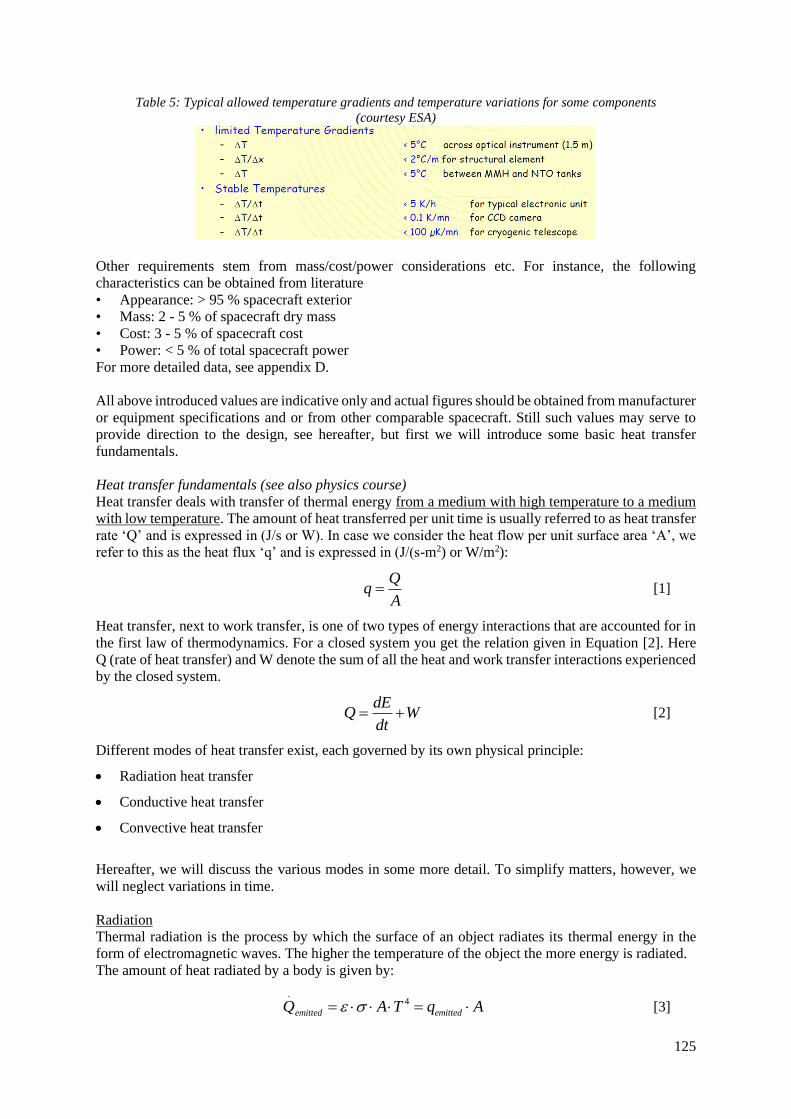
125
Table 5: Typical allowed temperature gradients and temperature variations for some components
(courtesy ESA)
Other requirements stem from mass/cost/power considerations etc. For instance, the following
characteristics can be obtained from literature
• Appearance: > 95 % spacecraft exterior
• Mass: 2 - 5 % of spacecraft dry mass
• Cost: 3 - 5 % of spacecraft cost
• Power: < 5 % of total spacecraft power
For more detailed data, see appendix D.
All above introduced values are indicative only and actual figures should be obtained from manufacturer
or equipment specifications and or from other comparable spacecraft. Still such values may serve to
provide direction to the design, see hereafter, but first we will introduce some basic heat transfer
fundamentals.
Heat transfer fundamentals (see also physics course)
Heat transfer deals with transfer of thermal energy from a medium with high temperature to a medium
with low temperature. The amount of heat transferred per unit time is usually referred to as heat transfer
rate ‘Q’ and is expressed in (J/s or W). In case we consider the heat flow per unit surface area ‘A’, we
refer to this as the heat flux ‘q’ and is expressed in (J/(s-m2) or W/m2):
Q
qA
= [1]
Heat transfer, next to work transfer, is one of two types of energy interactions that are accounted for in
the first law of thermodynamics. For a closed system you get the relation given in Equation [2]. Here
Q (rate of heat transfer) and W denote the sum of all the heat and work transfer interactions experienced
by the closed system.
dE
Q Wdt
= + [2]
Different modes of heat transfer exist, each governed by its own physical principle:
• Radiation heat transfer
• Conductive heat transfer
• Convective heat transfer
Hereafter, we will discuss the various modes in some more detail. To simplify matters, however, we
will neglect variations in time.
Radiation
Thermal radiation is the process by which the surface of an object radiates its thermal energy in the
form of electromagnetic waves. The higher the temperature of the object the more energy is radiated.
The amount of heat radiated by a body is given by:
.
4
emittedemittedQ A T q A = = [3]

126
• = emissivity of a body (0< < 1). It depends on the material, wavelength and temperature of a
body. An object is called a black body radiator if = 1 (for all wavelengths)
• = Stefan Boltzmann constant ( = 5.67 x 10⁻⁸ W/m2-K4)
• A = radiating area of body
• T = body temperature
• q = heat flux
Conduction
Conduction takes place in stationary mediums such as solids, liquids, and gases due to a temperature
gradient. Heat flows through thermally conductive materials by a process generally known as 'gradient
transport'. It depends on three quantities: the conductivity of the material, the cross-sectional area of the
material, and the spatial gradient of temperature. Conductive heat transfer is mathematically best
described by Fourier’s law, which quantifies the conduction process as a rate equation in three
dimensions. To simplify matters, the discussion hereafter will be limited to uni-directional conduction,
i.e. conduction in one direction only. For stationary conditions, you get the relation given in Equation
[4], where k is the coefficient of thermal conductivity [W/mK], A the cross sectional area [m2], and l
the length of conductive path [m]. Of these, the thermal conductivity coefficient depends on the material
selected.
( ).
2 1
k A k AQ T T T
l l
= = − [4]
From this relationship, we learn that the larger the conductivity, and/or the temperature gradient the
faster the heat flow. It is mentioned that heat transfer takes place in the direction of decreasing
temperature; a negative sign in the answer than indicates that the heat flow is from location 1 to 2 instead
of the other way around. The thermal conductivity is a measure of how efficiently a solid conducts heat
or how fast heat travels through the material.
Convection
“Convection” is energy transfer between a solid surface and an adjacent moving gas or liquid, i.e. the
transport of heat by a moving fluid (liquid or gas). It basically results from a combination of diffusion
or molecular motion within the fluid and the bulk or macroscopic motion of the fluid. For convection
you get the relation given in Equation [5], where hc is the coefficient of convective heat transfer
[W/m2K], A the surface area in contact with the flow [m2], and T the temperature difference [K]
between body and the surrounding medium.
.
cQ h T A= [5]
The spacecraft thermal environment
Since the spacecraft is in space and space essentially is empty, we do not have to worry about heat
flowing to the spacecraft either by convection nor conduction. Some convection/conduction may occur
at low altitudes (consider vehicles entering a planetary atmosphere), but this is considered out of scope.
Note that inside the spacecraft conduction and convection may take place next to radiation heat transfer.
For now though we will only consider the interaction of the spacecraft with the space environment. This
interaction is shown in Figure 1 for a spacecraft nearby Earth.

127
From Figure 1 we learn that there are essentially 3 flows of heat to the spacecraft and 1 flow away from
it. The incoming heat flow consists of (direct) solar radiation from the Sun (except when it experiences
an eclipse), solar energy reflected from the
surface in the direction of the spacecraft
(again except when it is experiencing an
eclipse), also referred to as albedo radiation.
In addition, because also the planet itself has
some temperature, the spacecraft may also
receive heat from the planet (planetary of IR
radiation). Not shown in the figure is that the
spacecraft itself serves as a source of heat,
thereby causing its temperature to rise.
Figure 1: Typical spacecraft thermal
environment [Fortescue]
Because space itself is a very cold environment (4 K) some heat will also be radiated away from the
spacecraft to the cold environment.
Hereafter, we will discuss the various heat flows in some more detail, before discussing how they affect
spacecraft temperature.
Solar intensity
One thing we all know is that the Sun is extremely hot with an effective radiating temperature of about
5780 K, where the effective radiating temperature of a celestial body is determined using relation [3]
under the assumption that = 1. It follows:
4= emittedq T [6]
And hence:
4= emittede
qT
[7]
From measurements we know that the flux emitted by the Sun at its surface is about 63.28 MW/m2.
This gives an effective temperature of our Sun of about 5780 K.
Using information on the radius of the Sun, we are able to determine that the total power emitted by the
Sun (P) is 3.856 x 1026 W. From conservation of energy, under the condition that energy is emitted
equally in all direction, see the sketch, it follows that the flux (also referred to as intensity) reduces with
the square of the distance to the center of the radiating object (inverse square law1).
1 From Wikipedia: In physics, an inverse-square law is any physical law stating that a specified physical
quantity or strength is inversely proportional to the square of the distance from the source of that physical
quantity.
Outer space is colder than the North Pole in December! But it can also be hotter than an erupting
Volcano. On Earth, air helps even out the temperature. But there is no air in space. You can fry on one
side while freezing on the other.
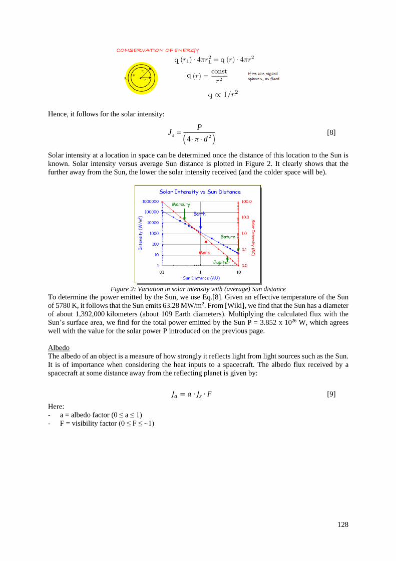
128
Hence, it follows for the solar intensity:
( )24
s
PJ
d=
[8]
Solar intensity at a location in space can be determined once the distance of this location to the Sun is
known. Solar intensity versus average Sun distance is plotted in Figure 2. It clearly shows that the
further away from the Sun, the lower the solar intensity received (and the colder space will be).
Figure 2: Variation in solar intensity with (average) Sun distance
To determine the power emitted by the Sun, we use Eq.[8]. Given an effective temperature of the Sun
of 5780 K, it follows that the Sun emits 63.28 MW/m2. From [Wiki], we find that the Sun has a diameter
of about 1,392,000 kilometers (about 109 Earth diameters). Multiplying the calculated flux with the
Sun’s surface area, we find for the total power emitted by the Sun P = 3.852 x 1026 W, which agrees
well with the value for the solar power P introduced on the previous page.
Albedo
The albedo of an object is a measure of how strongly it reflects light from light sources such as the Sun.
It is of importance when considering the heat inputs to a spacecraft. The albedo flux received by a
spacecraft at some distance away from the reflecting planet is given by:
𝐽𝑎 = 𝑎 ∙ 𝐽𝑠 ∙ 𝐹 [9]
Here:
- a = albedo factor (0 ≤ a ≤ 1)
- F = visibility factor (0 ≤ F ≤ ~1)
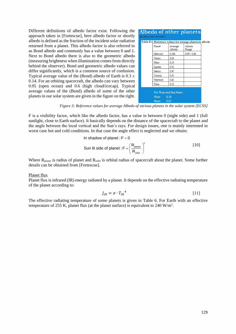
129
Different definitions of albedo factor exist. Following the
approach taken in [Fortescue], here albedo factor or shortly
albedo is defined as the fraction of the incident solar radiation
returned from a planet. This albedo factor is also referred to
as Bond albedo and commonly has a value between 0 and 1.
Next to Bond albedo there is also to the geometric albedo
(measuring brightness when illumination comes from directly
behind the observer). Bond and geometric albedo values can
differ significantly, which is a common source of confusion.
Typical average value of the (Bond) albedo of Earth is 0.3 ±
0.14. For an orbiting spacecraft, the albedo can vary between
0.05 (open ocean) and 0.6 (high cloud/icecap). Typical
average values of the (Bond) albedo of some of the other
planets in our solar system are given in the figure on the right.
Figure 3: Reference values for average Albedo of various planets in the solar system [ECSS]
F is a visibility factor, which like the albedo factor, has a value in between 0 (night side) and 1 (full
sunlight, close to Earth surface). It basically depends on the distance of the spacecraft to the planet and
the angle between the local vertical and the Sun’s rays. For design issues, one is mainly interested in
worst case hot and cold conditions. In that case the angle effect is neglected and we obtain:
2
planet
orbit
In shadow of planet : F 0
RSun lit side of planet : F
R
=
=
[10]
Where Rplanet is radius of planet and Rorbit is orbital radius of spacecraft about the planet. Some further
details can be obtained from [Fortescue].
Planet flux
Planet flux is infrared (IR) energy radiated by a planet. It depends on the effective radiating temperature
of the planet according to:
𝐽𝐼𝑅 = 𝜎 ∙ 𝑇𝐼𝑅4 [11]
The effective radiating temperature of some planets is given in Table 6. For Earth with an effective
temperature of 255 K, planet flux (at the planet surface) is equivalent to 240 W/m2.

130
Table 6: Effective radiating temperature of the planets of the solar system [ECSS]
Celestial body
Effective radiating
temperature
[K] Sun 5780
Mercury 600-617 Venus 227
Earth 255 Moon 120-380
Mars 210.1 Jupiter 109.5
Saturn 81.1 Uranus 58.2
Neptune 46.6 Pluto 43
For the Moon values are given for the sun lit side and for the night side independently.
Like for solar intensity, IR intensity is inversely proportional to the square of the radiating planet. This
makes that in deep space planet IR flux is (almost) negligible.
Heat fluxes as calculated for a real mission
Figure 4 shows how the heat fluxes may vary for a real space mission, in this case a mission to the
Moon. When in full sunlight close to Earth, the S/C may experience a heat flux of about 1700 W/m2
whereas in Earth shadow, it is just about 70 W/m2. In Moon orbit the numbers are again quite
different.
Figure 4: Overview of heat fluxes as experienced for the M3 mission
Students should prepare for calculating the heat fluxes for different spacecraft under different conditions.
Temperature change
The heat flowing to the spacecraft will cause a rise in temperature (T) of the spacecraft. The
temperature rise can be calculated using Eq.[12], where Q is heat flow rate (in Watt), t is time period
considered, M is mass of body and C is heat capacity of the body.
.
Q tT
M C
=
[12]
131
Example: spacecraft heating
Consider a spacecraft at a distance of 1 AU from the Sun. This spacecraft has a mass of 500 kg and a
heat capacity of 1000 J/kg-K. The area of the spacecraft receiving the solar flux is 2 m2. Determine for
this spacecraft the rise in temperature in case the spacecraft is exposed to the Sun for a duration of 1 hour (note other heat flows may be neglected).
Solution:
Heat flow to the spacecraft is 2.8 kJ/s. This gives a temperature rise of the spacecraft:
( )
2.8 [kJ/s] 3600 [s]20.2 [K]
500 [kg] 1000 [J/kg-K]T
= =
The problem gets even worse, when considering that onboard of the S/C we have a number of instruments and equipment that dissipate energy and hence generate heat. Typical electrical efficiencies of most
equipment are in the range of 15-30%. The remainder is lost in terms of heat.
Still, most preliminary thermal analysis is performed neglecting any changes in time. Changes in time
will only be considered when detailing the design. More important is to consider equilibrium conditions,
wherein the heat flowing to the spacecraft balances with the heat flowing away from the spacecraft.
Heat balance
The interplay of energy exchange between two bodies is characterized by Eq.[13], where presents
spectral absorption factor, spectral reflection factor and spectral transmission factor. These
parameters all depend on the material used, the wavelength considered and the temperature. The spectral
absorption factor of some material at some wavelength is equal to its emissivity; this relation is known
as Kirchhoff's law of thermal radiation. Consequently for a black body also = 1.
1 + + = [13]
In a practical situation a spacecraft receives thermal energy from the Sun. When in the vicinity of a
planet, the spacecraft may also receive reflected sun light and IR radiation from the planet itself.
However, the spacecraft also loses considerable energy by emitting infrared heat, as shown in
[Fortescue, Figure 11.1]. It will experience thermal equilibrium once the flow of energy to the spacecraft
(including the heat internally generated on board) balances with the heat flow from the spacecraft to
outer space. It follows:
= = + =in out absorbed dissipated emittedQ Q Q P Q [14]
The amount of heat absorbed by the spacecraft is given by the following equations:
.
= + + s s i s a i IR IR iabsorbedQ J A J A J A [15]
( ).
= + + =s s i s a i IR IR i IR IRabsorbedQ J A J A J A [16]
Where:
• is emissivity
• = absorptivity
• J = intensity
• Subscripts s, a and IR refer to solar radiation, albedo and IR radiation, respectively
• Ai = projected area receiving respectively solar, albedo and planetary radiation. Respective areas
vary depending on the vehicle orientation to the oncoming radiation. Subscript “I” refers to
incoming radiation.

132
Note that in relation [15] different absorption factors apply for solar radiation and Earth IR. This is
because the radiation from the Sun and the Earth IR encompass different frequencies. In relation [16],
the absorptivity in the IR range is set equal to the emissivity in the IR range. This is because according
Kirchhoff, absorptivity and emissivity of a material at identical temperature are essentially equal. Now
in spacecraft thermal engineering, we like to get rid of the subscripts “IR” and “s” and hence the thermal
jargon uses:
o for absorption in solar spectrum
o for absorption and emission in infrared spectrum
Another important heat source is the heat internally generated in the spacecraft by the various devices,
like batteries, power converters, etc., represented by (dissipated
P ). The summation sign here signifies
that heat may be dissipated in multiple devices.
The heat flowing away from the spacecraft can be determined using:
.
4= IR eemittedQ A T [17]
Here the subscript “e” denotes the emitting surface, which may be quite different from the surface
receiving radiation, see for instance the example below.
Example: Equilibrium temperature flat plate
A flat plate at 1 AU from the Sun is illuminated by the Sun with the Sun’s rays normally incident to the
flat plate. In equilibrium, it follows that the energy absorbed equals the energy emitted:
4 4
= → =
s a ss a s IR e
IR e
A JA J A T T
A
• Aa = area receiving/absorbing sunlight, Ae is radiating area = 2 Aa
• Black on both sides: (s IR = 0.9/0.85 )
• Js = 1371 W/m2
Filling in numbers provides an equilibrium temperature for the plate of 63oC.
The thermal control subsystem
The thermal control subsystem consists of all the hardware (and software) needed to maintain the
temperatures of all spacecraft bus components, and those payload suites without their own thermal
control provisions, within acceptable limits during ground test, launch and on orbit operations.
For instance, the equilibrium temperature for the flat plate type calculated in the foregoing example
may be lowered by selecting a larger area for radiating heat away. Another option might be to select
materials with a different ratio between solar absorptance and IR emissivity, see for instance Table 7.
Table 7: Solar absorptance and hemispherical emissivity of typical space materials
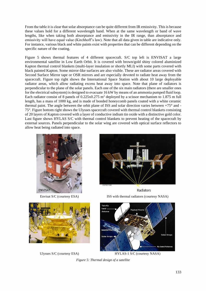
133
From the table it is clear that solar absorptance can be quite different from IR emissivity. This is because
these values hold for a different wavelength band. When at the same wavelength or band of wave
lengths, like when taking both absorptance and emissivity in the IR range, than absorptance and
emissivity will have equal value (Kirchhoff’s law). Note that all data given in table are indicative only.
For instance, various black and white paints exist with properties that can be different depending on the
specific nature of the coating.
Figure 5 shows thermal features of 4 different spacecraft. S/C top left is ENVISAT a large
environmental satellite in Low Earth Orbit. It is covered with brown/gold shiny colored aluminized
Kapton thermal control blankets (multi-layer insulation or shortly MLI) with some parts covered with
black painted Kapton. Some mirror-like surfaces are also visible. These are radiator areas covered with
Second Surface Mirror tape or OSR mirrors and are especially devoted to radiate heat away from the
spacecraft. Figure top right shows the International Space Station with about 10 large deployable
radiator areas, which allow radiating excess heat away into space. Note that plane of radiators is
perpendicular to the plane of the solar panels. Each one of the six main radiators (there are smaller ones
for the electrical subsystem) is designed to evacuate 16 kW by means of an ammonia pumped fluid loop.
Each radiator consist of 8 panels of 0.225x0.275 m2 deployed by a scissor mechanism to 1.875 m full
length, has a mass of 1000 kg, and is made of bonded honeycomb panels coated with a white ceramic
thermal paint. The angle between the orbit plane of ISS and solar direction varies between +75° and -
75°. Figure bottom right shows the Ulysses spacecraft covered with thermal control blankets consisting
of 20 layers of Kapton covered with a layer of conductive indium tin oxide with a distinctive gold color.
Last figure shows HYLAS S/C with thermal control blankets to prevent heating of the spacecraft by
external sources. Panels perpendicular to the solar wing are covered with optical surface reflectors to
allow heat being radiated into space.
Envisat S/C (courtesy ESA)
ISS with thermal radiators (courtesy NASA)
Ulysses S/C (courtesy ESA) HYLAS-1 S/C (courtesy NASA)
Figure 5: Thermal design of a satellite
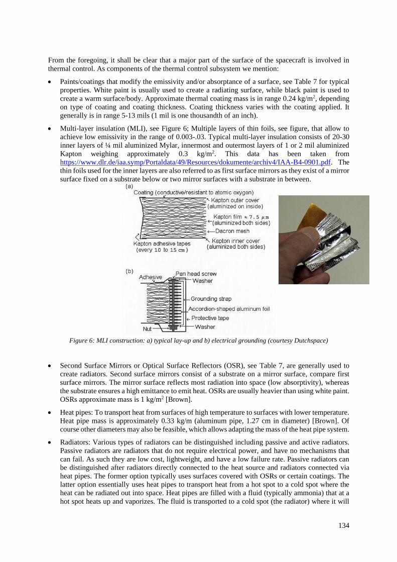
134
From the foregoing, it shall be clear that a major part of the surface of the spacecraft is involved in
thermal control. As components of the thermal control subsystem we mention:
• Paints/coatings that modify the emissivity and/or absorptance of a surface, see Table 7 for typical
properties. White paint is usually used to create a radiating surface, while black paint is used to
create a warm surface/body. Approximate thermal coating mass is in range 0.24 kg/m2, depending
on type of coating and coating thickness. Coating thickness varies with the coating applied. It
generally is in range 5-13 mils (1 mil is one thousandth of an inch).
• Multi-layer insulation (MLI), see Figure 6; Multiple layers of thin foils, see figure, that allow to
achieve low emissivity in the range of 0.003-.03. Typical multi-layer insulation consists of 20-30
inner layers of ¼ mil aluminized Mylar, innermost and outermost layers of 1 or 2 mil aluminized
Kapton weighing approximately 0.3 kg/m2. This data has been taken from
https://www.dlr.de/iaa.symp/Portaldata/49/Resources/dokumente/archiv4/IAA-B4-0901.pdf. The
thin foils used for the inner layers are also referred to as first surface mirrors as they exist of a mirror
surface fixed on a substrate below or two mirror surfaces with a substrate in between.
Figure 6: MLI construction: a) typical lay-up and b) electrical grounding (courtesy Dutchspace)
• Second Surface Mirrors or Optical Surface Reflectors (OSR), see Table 7, are generally used to
create radiators. Second surface mirrors consist of a substrate on a mirror surface, compare first
surface mirrors. The mirror surface reflects most radiation into space (low absorptivity), whereas
the substrate ensures a high emittance to emit heat. OSRs are usually heavier than using white paint.
OSRs approximate mass is 1 kg/m2 [Brown].
• Heat pipes: To transport heat from surfaces of high temperature to surfaces with lower temperature.
Heat pipe mass is approximately 0.33 kg/m (aluminum pipe, 1.27 cm in diameter) [Brown]. Of
course other diameters may also be feasible, which allows adapting the mass of the heat pipe system.
• Radiators: Various types of radiators can be distinguished including passive and active radiators.
Passive radiators are radiators that do not require electrical power, and have no mechanisms that
can fail. As such they are low cost, lightweight, and have a low failure rate. Passive radiators can
be distinguished after radiators directly connected to the heat source and radiators connected via
heat pipes. The former option typically uses surfaces covered with OSRs or certain coatings. The
latter option essentially uses heat pipes to transport heat from a hot spot to a cold spot where the
heat can be radiated out into space. Heat pipes are filled with a fluid (typically ammonia) that at a
hot spot heats up and vaporizes. The fluid is transported to a cold spot (the radiator) where it will
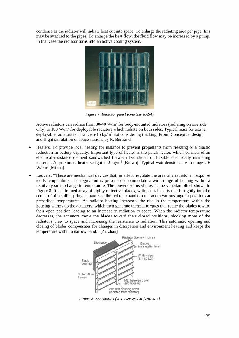
135
condense as the radiator will radiate heat out into space. To enlarge the radiating area per pipe, fins
may be attached to the pipes. To enlarge the heat flow, the fluid flow may be increased by a pump.
In that case the radiator turns into an active cooling system.
Figure 7: Radiator panel (courtesy NASA)
Active radiators can radiate from 30-40 W/m2 for body-mounted radiators (radiating on one side
only) to 180 W/m2 for deployable radiators which radiate on both sides. Typical mass for active,
deployable radiators is in range 5-15 kg/m2 not considering tracking. From: Conceptual design
and flight simulation of space stations by R. Bertrand.
• Heaters: To provide local heating for instance to prevent propellants from freezing or a drastic
reduction in battery capacity. Important type of heater is the patch heater, which consists of an
electrical-resistance element sandwiched between two sheets of flexible electrically insulating
material. Approximate heater weight is 2 kg/m2 [Brown]. Typical watt densities are in range 2-6
W/cm2 [Minco].
• Louvers: “These are mechanical devices that, in effect, regulate the area of a radiator in response
to its temperature. The regulation is preset to accommodate a wide range of heating within a
relatively small change in temperature. The louvers set used most is the venetian blind, shown in
Figure 8. It is a framed array of highly reflective blades, with central shafts that fit tightly into the
center of bimetallic spring actuators calibrated to expand or contract to various angular positions at
prescribed temperatures. As radiator heating increases, the rise in the temperature within the
housing warms up the actuators, which then generate thermal torques that rotate the blades toward
their open position leading to an increase in radiation to space. When the radiator temperature
decreases, the actuators move the blades toward their closed positions, blocking more of the
radiator's view to space and increasing the resistance to radiation. This automatic opening and
closing of blades compensates for changes in dissipation and environment heating and keeps the
temperature within a narrow band.” [Zarchan]
Figure 8: Schematic of a louver system [Zarchan]
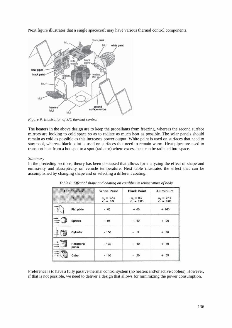
136
Next figure illustrates that a single spacecraft may have various thermal control components.
Figure 9: Illustration of S/C thermal control
The heaters in the above design are to keep the propellants from freezing, whereas the second surface
mirrors are looking to cold space so as to radiate as much heat as possible. The solar panels should
remain as cold as possible as this increases power output. White paint is used on surfaces that need to
stay cool, whereas black paint is used on surfaces that need to remain warm. Heat pipes are used to
transport heat from a hot spot to a spot (radiator) where excess heat can be radiated into space.
Summary
In the preceding sections, theory has been discussed that allows for analyzing the effect of shape and
emissivity and absorptivity on vehicle temperature. Next table illustrates the effect that can be
accomplished by changing shape and or selecting a different coating.
Table 8: Effect of shape and coating on equilibrium temperature of body
Preference is to have a fully passive thermal control system (no heaters and/or active coolers). However,
if that is not possible, we need to deliver a design that allows for minimizing the power consumption.

137
Problems
1. The black body or effective radiating temperature of the Sun is ~5780 K. The Sun has a radius of
6.955E8 m. Determine:
a. Total power emitted by the Sun.
b. Solar flux at the surface of the Sun
c. Solar flux at a distance of 1 AU
Answers: a) 3.847E26 W, b) 63.3 MW/m2, c) 1368 W/m2
2. Consider that the average solar flux received by Earth is 1368 W/m2. Earth albedo is 0.33 and the
heat produced by Earth itself (volcanoes, Earth power plants, etc.) is negligibly small. Determine:
a. effective radiating (or equilibrium) temperature of Earth.
b. incident IR flux on a spacecraft in circular orbit at an altitude of 900 km (hint: Earth radius
is 6371 km)
Answer: a) 255 K, b) 184.1 W/m2
3. A cubic spacecraft of linear dimension 2 m has a temperature of 300 K. Determine total power
emitted by the S/C in case the S/C is covered by a material with emissivity 0.6.
Answer: 6.6 kW (S/C surface area that radiates heat is 24 m2 (6 sides of 2 x 2 m2 each)
4. Solar flux received by Earth is 1368 W/m2. Earth albedo is 0.3. Determine:
A. Transmission and absorption factor of Earth for solar radiation
B. Maximum albedo flux incident on spacecraft in a 1000 km altitude circular orbit about
Earth considering a view factor F equal to 1.
C. Same question as under B for an orbital altitude of 10,000 km. Use a more realistic estimate
for F (you may assume that the local vertical coincides with the Sun’s rays)
Answers:
A) Transmission factor = 0 and absorption factor = 0.7
B) Albedo flux is 1368 W/m2 x 0.3 x 1 = 410 W/m2
C) 62 W/m2 (F = (6371km/16371km)2 = 0.15 => 1368 W/m2 x 0.3 x 0.15)
5. Consider a spherical shaped S/C in Earth orbit. The S/C is covered with a black paint with an
absorption factor of 0.96 and an emission factor of 0.75. Calculate for this S/C its equilibrium
temperature in full sunlight under the assumption that albedo, IR and internal heat dissipation are
negligible.
Answer: 297 K
6. Consider a spherical spacecraft of diameter 2 m in a 1000 km circular orbit about Earth. This
spacecraft has a solar absorptivity of 0.4 and an IR emissivity of 0.2. Summed internal heat
dissipation of all instruments is 150 W. Furthermore are given an Earth albedo of 0.3 and a solar
flux at 1 AU of 1368 W/m2. Determine:
A. Solar flux incident on S/C
B. IR flux incident on S/C
C. Maximum albedo flux incident on S/C
D. Hot case equilibrium temperature of the S/C (S/C in full sunlight, full visibility)
E. Cold case equilibrium temperature of the S/C (S/C in Earth shadow, no internal heat
dissipation)
Answers: A) 1368 W/m2, B) 179 W/m2, C) 410 W/m2 ( F = 1), D) 364 K, E) 168 K
138
7. Consider a solar wing of a spacecraft. This wing is producing electrical power at a distance of 4.4
AU from the sun. Its frontal area (area covered with solar cells) is 10 m2.
• Solar incidence angle is normal to the solar panel
• Solar flux at 1 AU is 1400 W/m2
• alpha/epsilon ratio of the solar cells (illuminated side) is 0.8/0.7
• alpha/epsilon ratio of the back of the panel is 0.5/0.7
• Panel is thermally insulated from the spacecraft with the back essentially seeing cold space
only
• Panel produces 108 W electrical power
Determine for this solar wing the equilibrium temperature under the given conditions.
Answer: 156 K.
Note that for an active solar panel (i.e. the panel is generating electric power), some of the power
absorbed by the panel is converted into electrical power (Pelectric) and hence the power balance
governing the calculation of the wing temperature should be written as:
�̇�𝑎𝑏𝑠𝑜𝑟𝑏𝑒𝑑 + ∑ 𝑃𝑑𝑖𝑠𝑠𝑖𝑝𝑎𝑡𝑒𝑑 = �̇�𝑒𝑚𝑖𝑡𝑡𝑒𝑑 + 𝑃𝑒𝑙𝑒𝑐𝑡𝑟𝑖𝑐
8. Consider a space probe in orbit about the planet Mercury. Mercury is close to the Sun with a closest
distance of 0.3 AU. Because of this close distance to the Sun, the probe will run hot. To prevent the
probe from getting too hot, it is shielded by a thermal shield. This question is about the maximum
equilibrium temperature the probe will attain even though when protected by the thermal shield.
Given are:
• Probe has a cylindrical planform
• Shield has a semi-cylindrical planform of same cylinder height as the probe
• Probe and shield have identical radius; there exists a tiny gap in between probe and shield as
to prevent heat conduction between the two, but this is not of importance for area calculation
of probe and shield
• Only solar radiation is considered (no albedo or Mercury IR)
• Solar radiation is perpendicular to shield cross-sectional area
• Probe is fully shielded
• Shield is coated on side facing the Sun with white paint with being 0.15/0.9
• Shield is coated on back side with coating that provides being 0.2/0.8
You are to determine the equilibrium temperature of the shield/probe for the following cases:
a) The equilibrium temperature of the shield in case the back of the shield sees only cold space
(this is not true, but allows to get an idea of the minimum shield temperature feasible). In this
case the presence of the probe itself is neglected.
b) The equilibrium temperature of the probe itself assuming that the presence of the probe does
not affect the shield temperature, all heat radiated at the back of the shield flows to the S/C
body and that the cylindrical probe sees only cold space (again, this is a simplification, but
allows to find a first temperature for the probe itself. The resulting temperature is considered to
be an ideal lower temperature value for the probe).
Answers: a) 350.2 K (solar intensity at 1 AU is taken equal to 1367 W/m2), b) 278.2 K
Further problems for exercising upon are available via the course web pages (look for Mobius
exercises) or can be found in the tutorial material.

139
6.4 Spacecraft Subsystems: Electrical Power Generation
The electrical power subsystem provides the spacecraft with the necessary electrical power over the
duration of the mission. Key requirements for the Electric Power System (EPS) are hence power level
and duration of power delivery.
Why electrical power
Most spacecraft need some means of electrical power provision to power the payloads, like:
o Radar transmitters and receivers
o Radio transmitters & receivers
o Visual (VIS), Infra-Red (IR), Ultra-Violet (UV) and roentgen (X-ray) cameras
and on-board equipment, like:
o Computer, data recorder
o Telemetry and -command radio transmitters & receivers
o Valves, pressure regulators
o Heaters
o Sensors (gyros, accelerometers, sun/star/Earth sensors, etc.), actuators (reaction wheels, momentum
wheels, etc.)
o Electrical motors
Electrical Power subsystem requirements
An important requirement for the electrical power subsystem is how much power, i.e. energy per unit
of time, is to be provided. As in the early design stages very little data is available one generally uses
any available information to come up with a first guestimate. For instance, Table 9 provides an overview
of installed power per mission type [ESA bulletin 87].
Table 9: Overview of installed power per mission type
Mission Orbit, Attitude Installed Power
(W) min-max
Science:
− Astronomy
− Deep space
HEO, Fixed point Sun pointing (mostly)
Various transfer orbits, Sun or planet pointing
200-1500
Telecommunication GEO, Earth pointing 500-5000
Earth Observation LEO, Earth pointing 500-5000
Meteorology GEO, Earth pointing 200-1500
Manned Vehicles Transfer + LEO, Various 1000-10000
Manned Stations LEO, Sun pointing 3000-30000
Now if the mission type is known, the above table can be used to come up with a first very global power
estimate. Still the uncertainty is quite large as is indicated by the large power range indicated in the
table. For instance, for science category spacecraft the mid-range value is 850 W, but apparently some
spacecraft will do with 200 W while others require 1500 W.
An alternative approach which allows for a more accurate estimate (and hence reducing power margin)
can be followed in case the electrical power usage of the payload is known. This is based on the
reasoning that payload power and total power generated are related. This approach has been described
in chapter 3 and is based on collecting (average on station) power data for comparable spacecraft, see
for instance the data collected in Table 1 and appendix B, and determining the relation that exists
between payload power and total generated power. A number of such relations have been collected in
Appendix C. These relations typically have a reasonable (but not perfect) estimation accuracy with an
RSE in the order of 20%. Because of the uncertainty one should take into account a reasonable margin
like for instance 2 RSE. The same approach of collecting data from similar historical spacecraft and
determining estimation relationships has been followed in generating a first power budget for the
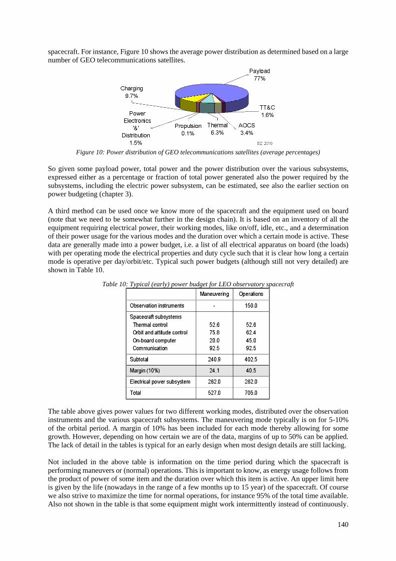
140
spacecraft. For instance, Figure 10 shows the average power distribution as determined based on a large
number of GEO telecommunications satellites.
Figure 10: Power distribution of GEO telecommunications satellites (average percentages)
So given some payload power, total power and the power distribution over the various subsystems,
expressed either as a percentage or fraction of total power generated also the power required by the
subsystems, including the electric power subsystem, can be estimated, see also the earlier section on
power budgeting (chapter 3).
A third method can be used once we know more of the spacecraft and the equipment used on board
(note that we need to be somewhat further in the design chain). It is based on an inventory of all the
equipment requiring electrical power, their working modes, like on/off, idle, etc., and a determination
of their power usage for the various modes and the duration over which a certain mode is active. These
data are generally made into a power budget, i.e. a list of all electrical apparatus on board (the loads)
with per operating mode the electrical properties and duty cycle such that it is clear how long a certain
mode is operative per day/orbit/etc. Typical such power budgets (although still not very detailed) are
shown in Table 10.
Table 10: Typical (early) power budget for LEO observatory spacecraft
The table above gives power values for two different working modes, distributed over the observation
instruments and the various spacecraft subsystems. The maneuvering mode typically is on for 5-10%
of the orbital period. A margin of 10% has been included for each mode thereby allowing for some
growth. However, depending on how certain we are of the data, margins of up to 50% can be applied.
The lack of detail in the tables is typical for an early design when most design details are still lacking.
Not included in the above table is information on the time period during which the spacecraft is
performing maneuvers or (normal) operations. This is important to know, as energy usage follows from
the product of power of some item and the duration over which this item is active. An upper limit here
is given by the life (nowadays in the range of a few months up to 15 year) of the spacecraft. Of course
we also strive to maximize the time for normal operations, for instance 95% of the total time available.
Also not shown in the table is that some equipment might work intermittently instead of continuously.
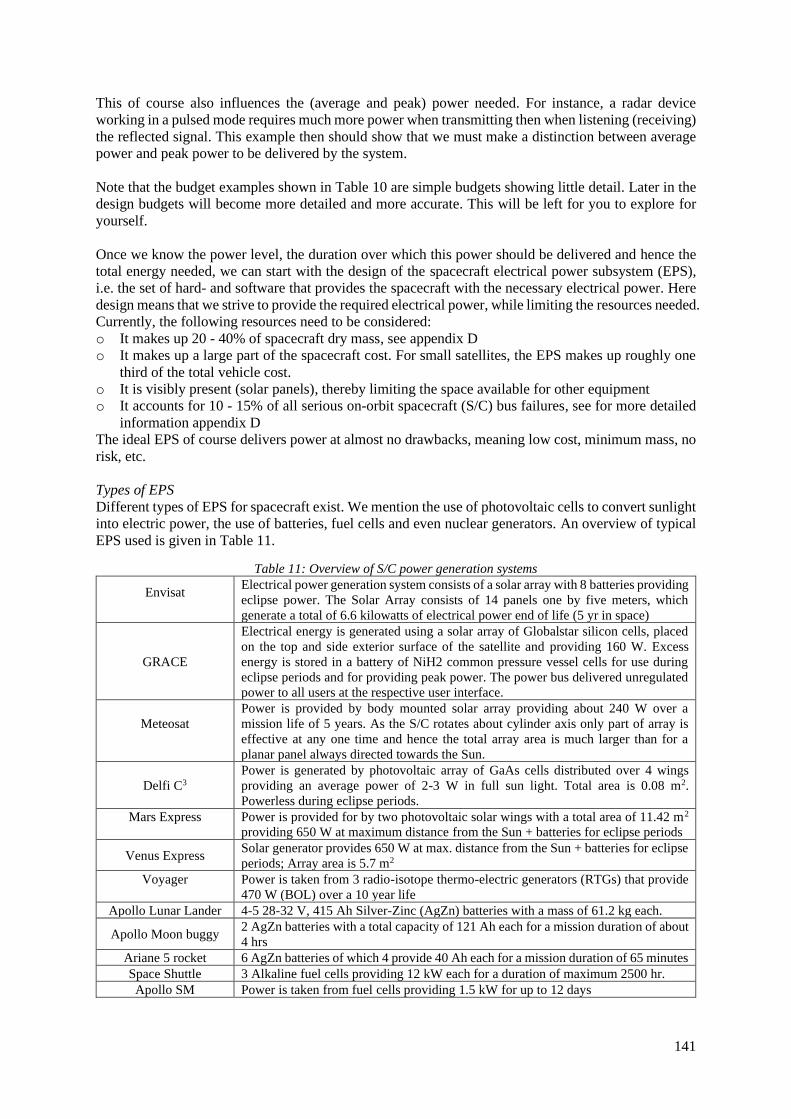
141
This of course also influences the (average and peak) power needed. For instance, a radar device
working in a pulsed mode requires much more power when transmitting then when listening (receiving)
the reflected signal. This example then should show that we must make a distinction between average
power and peak power to be delivered by the system.
Note that the budget examples shown in Table 10 are simple budgets showing little detail. Later in the
design budgets will become more detailed and more accurate. This will be left for you to explore for
yourself.
Once we know the power level, the duration over which this power should be delivered and hence the
total energy needed, we can start with the design of the spacecraft electrical power subsystem (EPS),
i.e. the set of hard- and software that provides the spacecraft with the necessary electrical power. Here
design means that we strive to provide the required electrical power, while limiting the resources needed.
Currently, the following resources need to be considered:
o It makes up 20 - 40% of spacecraft dry mass, see appendix D
o It makes up a large part of the spacecraft cost. For small satellites, the EPS makes up roughly one
third of the total vehicle cost.
o It is visibly present (solar panels), thereby limiting the space available for other equipment
o It accounts for 10 - 15% of all serious on-orbit spacecraft (S/C) bus failures, see for more detailed
information appendix D
The ideal EPS of course delivers power at almost no drawbacks, meaning low cost, minimum mass, no
risk, etc.
Types of EPS
Different types of EPS for spacecraft exist. We mention the use of photovoltaic cells to convert sunlight
into electric power, the use of batteries, fuel cells and even nuclear generators. An overview of typical
EPS used is given in Table 11.
Table 11: Overview of S/C power generation systems
Envisat
Electrical power generation system consists of a solar array with 8 batteries providing
eclipse power. The Solar Array consists of 14 panels one by five meters, which
generate a total of 6.6 kilowatts of electrical power end of life (5 yr in space)
GRACE
Electrical energy is generated using a solar array of Globalstar silicon cells, placed
on the top and side exterior surface of the satellite and providing 160 W. Excess
energy is stored in a battery of NiH2 common pressure vessel cells for use during
eclipse periods and for providing peak power. The power bus delivered unregulated
power to all users at the respective user interface.
Meteosat
Power is provided by body mounted solar array providing about 240 W over a
mission life of 5 years. As the S/C rotates about cylinder axis only part of array is
effective at any one time and hence the total array area is much larger than for a
planar panel always directed towards the Sun.
Delfi C3
Power is generated by photovoltaic array of GaAs cells distributed over 4 wings
providing an average power of 2-3 W in full sun light. Total area is 0.08 m2.
Powerless during eclipse periods.
Mars Express
Power is provided for by two photovoltaic solar wings with a total area of 11.42 m2
providing 650 W at maximum distance from the Sun + batteries for eclipse periods
Venus Express Solar generator provides 650 W at max. distance from the Sun + batteries for eclipse
periods; Array area is 5.7 m2
Voyager
Power is taken from 3 radio-isotope thermo-electric generators (RTGs) that provide
470 W (BOL) over a 10 year life
Apollo Lunar Lander 4-5 28-32 V, 415 Ah Silver-Zinc (AgZn) batteries with a mass of 61.2 kg each.
Apollo Moon buggy 2 AgZn batteries with a total capacity of 121 Ah each for a mission duration of about
4 hrs
Ariane 5 rocket 6 AgZn batteries of which 4 provide 40 Ah each for a mission duration of 65 minutes
Space Shuttle 3 Alkaline fuel cells providing 12 kW each for a duration of maximum 2500 hr.
Apollo SM Power is taken from fuel cells providing 1.5 kW for up to 12 days
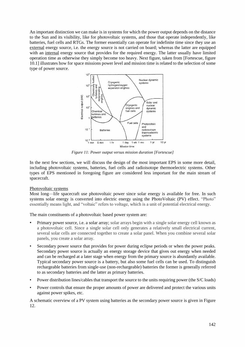
142
An important distinction we can make is in systems for which the power output depends on the distance
to the Sun and its visibility, like for photovoltaic systems, and those that operate independently, like
batteries, fuel cells and RTGs. The former essentially can operate for indefinite time since they use an
external energy source, i.e. the energy source is not carried on board; whereas the latter are equipped
with an internal energy source that provides for the required energy. The latter usually have limited
operation time as otherwise they simply become too heavy. Next figure, taken from [Fortescue, figure
10.1] illustrates how for space missions power level and mission time is related to the selection of some
type of power source.
Figure 11: Power output versus mission duration [Fortescue]
In the next few sections, we will discuss the design of the most important EPS in some more detail,
including photovoltaic systems, batteries, fuel cells and radioisotope thermoelectric systems. Other
types of EPS mentioned in foregoing figure are considered less important for the main stream of
spacecraft.
Photovoltaic systems
Most long—life spacecraft use photovoltaic power since solar energy is available for free. In such
systems solar energy is converted into electric energy using the PhotoVoltaic (PV) effect. “Photo”
essentially means light, and “voltaic” refers to voltage, which is a unit of potential electrical energy.
The main constituents of a photovoltaic based power system are:
• Primary power source, i.e. a solar array; solar arrays begin with a single solar energy cell known as
a photovoltaic cell. Since a single solar cell only generates a relatively small electrical current,
several solar cells are connected together to create a solar panel. When you combine several solar
panels, you create a solar array.
• Secondary power source that provides for power during eclipse periods or when the power peaks.
Secondary power source is actually an energy storage device that gives out energy when needed
and can be recharged at a later stage when energy from the primary source is abundantly available.
Typical secondary power source is a battery, but also some fuel cells can be used. To distinguish
rechargeable batteries from single-use (non-rechargeable) batteries the former is generally referred
to as secondary batteries and the latter as primary batteries.
• Power distribution lines/cables that transport the source to the units requiring power (the S/C loads)
• Power controls that ensure the proper amounts of power are delivered and protect the various units
against power spikes, etc.
A schematic overview of a PV system using batteries as the secondary power source is given in Figure
12.

143
Figure 12: Schematic of photo-voltaic based EPS
When starting the design of a PV system, it should be clear that we need to know about how much
power is needed and when. It should also be clear that we need to distinguish between two main
operating modes for the PV system; a first mode wherein the solar array is receiving sun light (sunlit
period) and provides power not only to the loads, i.e. the equipment requiring electrical power), but also
to the secondary power source for recharging and a second mode wherein the solar array is not operative
(when the array is shadowed by for instance Earth, see Figure 13.) and the required energy is drawn
from the secondary power source. Sometimes a third (peak power) mode is distinguished, wherein the
battery supports the primary power source to deliver peak power for those cases where the primary
energy source itself cannot deliver sufficient power. All these aspects should be taken into account by
the designer when designing an EPS system.
Figure 13: S/C experiencing solar eclipse during its rotation about some planet
Next relation illustrates how the power (P) that should be delivered by the solar array (SA) is determined
using an energy balance. The relation applies to a spacecraft in orbit about some planet with the
spacecraft experiencing sunlit and eclipse periods:
𝑃𝑆𝐴 ∙ 𝑡𝑑 =𝑃𝑑∙ 𝑡𝑑
𝜂𝑑+
𝑃𝑒∙ 𝑡𝑒
𝜂𝑒 [18]
Here t is time with the subscript d referring to the daytime period and e to the duration of the eclipse
period, Pd is the power needed during day time and Pe during eclipse and gives the path efficiency of
the power (control) system during day time and night time, respectively. Note that:
• Second term on right hand side (RHS) gives the total energy that should be provided for by the
battery even though the energy is delivered in the sunlit period.
• A distinction is made in the relationship between day time and night time power consumption.
This is because during night time one might operate only a limited set of equipment or at
reduced power to conserve energy.
• In the above relationship the day time and night time power are considered constant. Still, you
may also look at them as average power over the day and night time period, respectively.
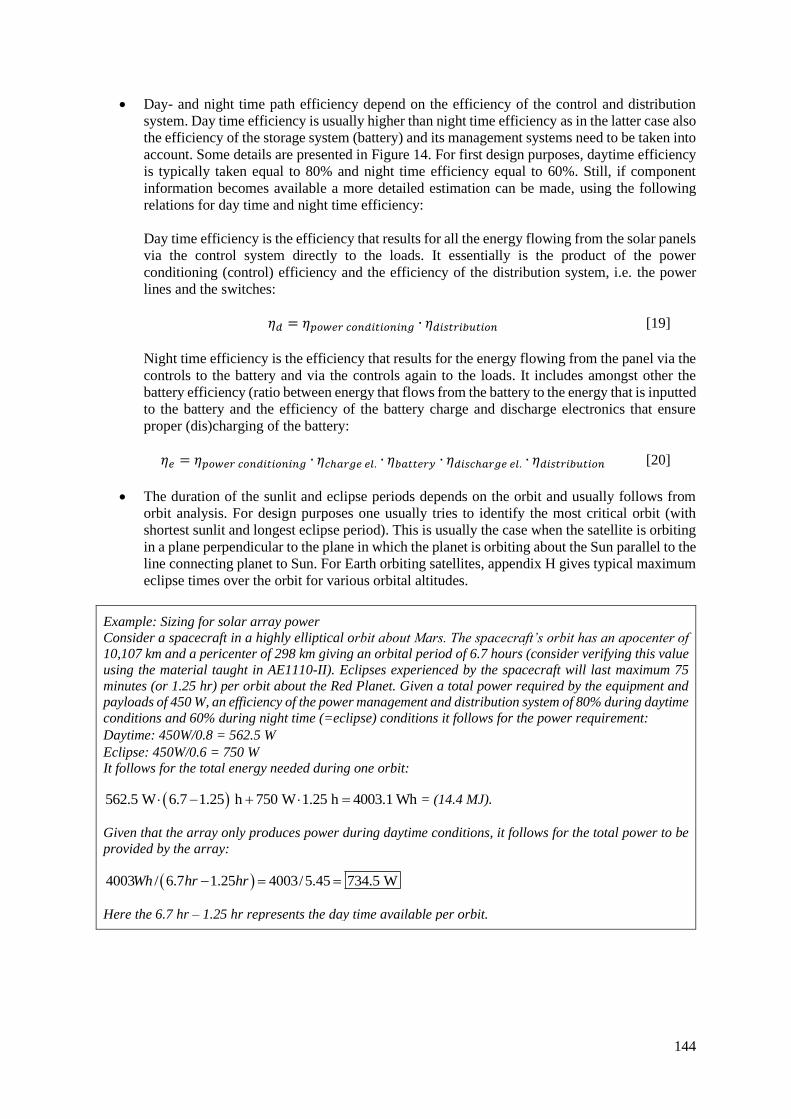
144
• Day- and night time path efficiency depend on the efficiency of the control and distribution
system. Day time efficiency is usually higher than night time efficiency as in the latter case also
the efficiency of the storage system (battery) and its management systems need to be taken into
account. Some details are presented in Figure 14. For first design purposes, daytime efficiency
is typically taken equal to 80% and night time efficiency equal to 60%. Still, if component
information becomes available a more detailed estimation can be made, using the following
relations for day time and night time efficiency:
Day time efficiency is the efficiency that results for all the energy flowing from the solar panels
via the control system directly to the loads. It essentially is the product of the power
conditioning (control) efficiency and the efficiency of the distribution system, i.e. the power
lines and the switches:
𝜂𝑑 = 𝜂𝑝𝑜𝑤𝑒𝑟 𝑐𝑜𝑛𝑑𝑖𝑡𝑖𝑜𝑛𝑖𝑛𝑔 ∙ 𝜂𝑑𝑖𝑠𝑡𝑟𝑖𝑏𝑢𝑡𝑖𝑜𝑛 [19]
Night time efficiency is the efficiency that results for the energy flowing from the panel via the
controls to the battery and via the controls again to the loads. It includes amongst other the
battery efficiency (ratio between energy that flows from the battery to the energy that is inputted
to the battery and the efficiency of the battery charge and discharge electronics that ensure
proper (dis)charging of the battery:
𝜂𝑒 = 𝜂𝑝𝑜𝑤𝑒𝑟 𝑐𝑜𝑛𝑑𝑖𝑡𝑖𝑜𝑛𝑖𝑛𝑔 ∙ 𝜂𝑐ℎ𝑎𝑟𝑔𝑒 𝑒𝑙. ∙ 𝜂𝑏𝑎𝑡𝑡𝑒𝑟𝑦 ∙ 𝜂𝑑𝑖𝑠𝑐ℎ𝑎𝑟𝑔𝑒 𝑒𝑙. ∙ 𝜂𝑑𝑖𝑠𝑡𝑟𝑖𝑏𝑢𝑡𝑖𝑜𝑛 [20]
• The duration of the sunlit and eclipse periods depends on the orbit and usually follows from
orbit analysis. For design purposes one usually tries to identify the most critical orbit (with
shortest sunlit and longest eclipse period). This is usually the case when the satellite is orbiting
in a plane perpendicular to the plane in which the planet is orbiting about the Sun parallel to the
line connecting planet to Sun. For Earth orbiting satellites, appendix H gives typical maximum
eclipse times over the orbit for various orbital altitudes.
Example: Sizing for solar array power
Consider a spacecraft in a highly elliptical orbit about Mars. The spacecraft’s orbit has an apocenter of 10,107 km and a pericenter of 298 km giving an orbital period of 6.7 hours (consider verifying this value
using the material taught in AE1110-II). Eclipses experienced by the spacecraft will last maximum 75
minutes (or 1.25 hr) per orbit about the Red Planet. Given a total power required by the equipment and payloads of 450 W, an efficiency of the power management and distribution system of 80% during daytime
conditions and 60% during night time (=eclipse) conditions it follows for the power requirement:
• Daytime: 450W/0.8 = 562.5 W
• Eclipse: 450W/0.6 = 750 W It follows for the total energy needed during one orbit:
( )562.5 W 6.7 1.25 h 750 W 1.25 h 4003.1 Wh − + = = (14.4 MJ).
Given that the array only produces power during daytime conditions, it follows for the total power to be
provided by the array:
( )4003 / 6.7 1.25 4003/5.45 734.5 WWh hr hr− = =
Here the 6.7 hr – 1.25 hr represents the day time available per orbit.
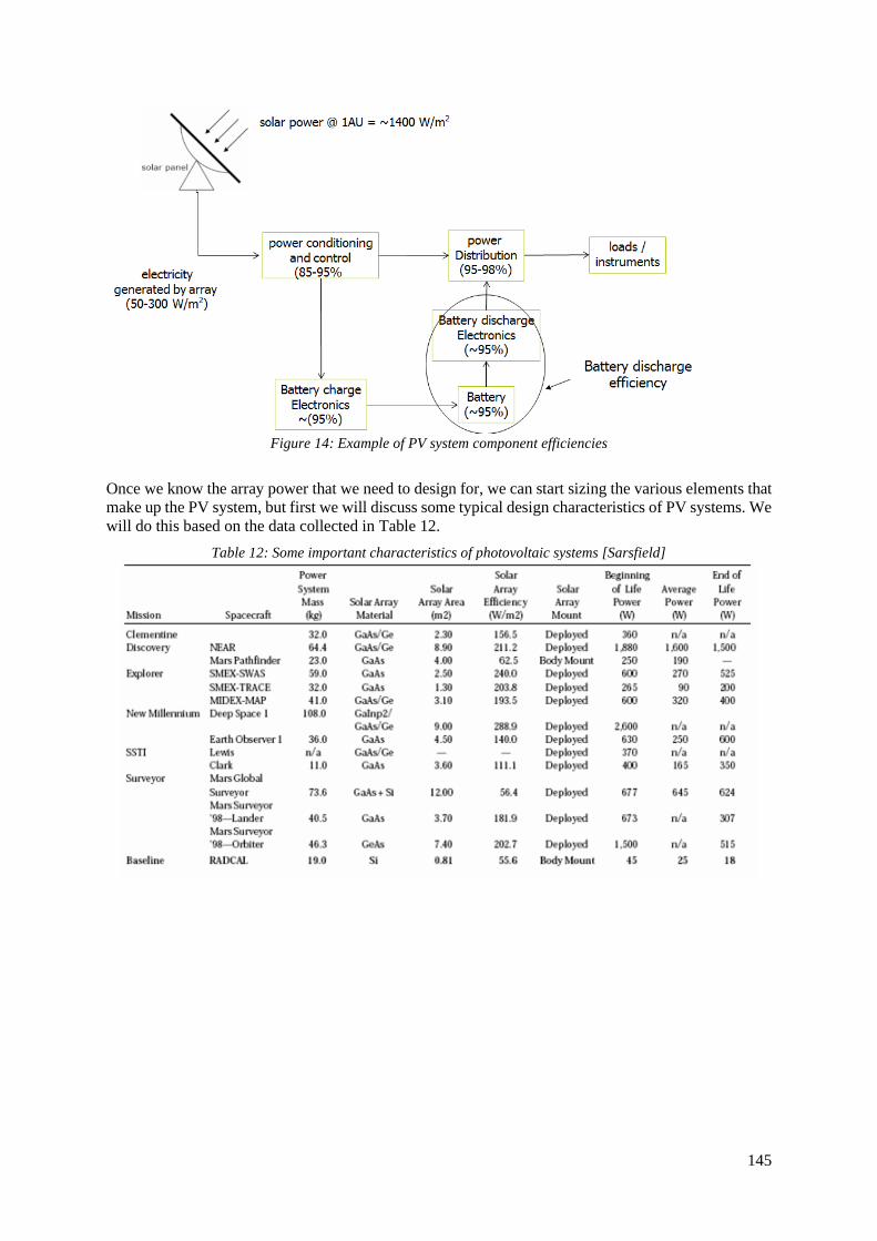
145
Figure 14: Example of PV system component efficiencies
Once we know the array power that we need to design for, we can start sizing the various elements that
make up the PV system, but first we will discuss some typical design characteristics of PV systems. We
will do this based on the data collected in Table 12.
Table 12: Some important characteristics of photovoltaic systems [Sarsfield]
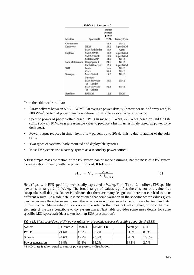
146
Table 12: Continued
From the table we learn that:
• Array delivers between 50-300 W/m2. On average power density (power per unit of array area) is
100 W/m2. Note that power density is referred to in table as solar array efficiency.
• Specific power of photo-voltaic based EPS is in range 1.0 W/kg - 25 W/kg based on End Of Life
(EOL) power (10 W/kg is a reasonable value to produce a first mass estimate based on power to be
delivered).
• Power output reduces in time (from a few percent up to 20%). This is due to ageing of the solar
cells.
• Two types of systems: body mounted and deployable systems
• Most PV systems use a battery system as a secondary power source.
A first simple mass estimation of the PV system can be made assuming that the mass of a PV system
increases about linearly with the power produced. It follows:
𝑀𝐸𝑃𝑆 = 𝑀𝑃𝑉 =𝑃𝑡𝑜𝑡𝑎𝑙
(𝑃𝑠𝑝)𝑠𝑦𝑠𝑡𝑒𝑚
[21]
Here (Psp)system is EPS specific power usually expressed in We/kg. From Table 12 it follows EPS specific
power is in range 2-40 We/kg. The broad range of values signifies there is not one value that
encapsulates all designs. Rather is indicates that there are many designs out there that can lead to quite
different results. As a side note it is mentioned that some variation in the specific power values given
may be because the solar intensity onto the array varies with distance to the Sun, see chapter 3 and later
in this chapter. Above relation is a very simple relation that does not tell anything on how the main
elements of the EPS contribute to the system mass. Next table provides some mass details for some
specific LEO spacecraft (data taken from an ESA presentation).
Table 13: Mass breakdown of PV power subsystem of specific spacecraft orbiting about Earth (ESA)
System Telecom 2 Jason 1 DEMETER Average STD
PMD* 21.6% 31.0% 38.2% 30.3% 8.3%
Storage 44.6% 35.7% 23.5% 34.6% 10.6%
Power generation 33.8% 33.3% 38.2% 35.1% 2.7%
* PMD mass is taken equal to sum of power system + distribution

147
Table also gives average mass percentages for the three main elements making up a PV system. To
generate the above table, it is assumed that the mass of the EPS is given as:
𝑀𝐸𝑃𝑆 = 𝑀𝑃𝑉 = 𝑀𝑆𝐴 + 𝑀𝐵𝐴𝑇 + 𝑀𝑃𝑀𝐷 [22]
Data in table agrees nicely with the EPS mass breakdown for PV systems for Earth satellites as shown
in Table 13. Still, the data also show that some spread does occur. This spread is signified by the
standard deviation (STD). This spread may be due to for instance orbital altitude or the orientation of
the orbital plane, etc. For instance, some satellites with long eclipses require a large and heavy battery
system whereas other can almost do without a battery system.
Figure 15: Typical photo-voltaic power subsystem mass breakdown (Earth satellites)
In the next few paragraphs a more detailed sizing of the EPS is discussed.
Array sizing
From the electrical power to be delivered by the array, the array can be sized and its mass determined.
The mass and size of the solar array can be determined using:
𝑀𝑆𝐴 =𝑃𝑆𝐴
(𝑃𝑠𝑝)𝑆𝐴
[23]
𝐴𝑆𝐴 =𝑃𝑆𝐴
(𝑃𝛿)𝑆𝐴 [24]
Here (Psp)SA is specific power of array (power/unit of solar array mass) and (P)SA is power density of
array (expressed in units of power per unit of array area), which both depend on the array type, see
Table 14.
Table 14: Space solar array types and their characteristics (values at 1 AU, normal incident radiation and BOL)
[Bailey]
Notice that the above relations have already been used in chapter 3 to generate a first estimate of solar
array size and mass. Note that array per power is inverse of the earlier introduced array power density.
That here the values for power density are much larger than the one used in chapter 3 is because in
chapter 3, low efficiency silicon was considered as baseline. Also the value used in chapter 3 holds for
End Of Life (EOL), whereas values given here are for Begin Of Life (BOL). The difference is that
148
during their life, solar arrays tend to degrade thereby producing less and less power. Typical values for
life degradation in GEO are:
−
Si array : 4% per year
GaAs array : 1 1.5% per year
Multi-junction GaAs: 0.5% per year
[25]
Actual values may be quite different and depend on the radiation environment, but above values allow
for a conservative estimate. Once the degradation is known, the power at BOL can be determined based
on known power at EOL and degradation rate. It follows:
𝑑𝑃
𝑑𝑡= −𝑑𝑒𝑔𝑟𝑎𝑑𝑎𝑡𝑖𝑜𝑛 𝑓𝑎𝑐𝑡𝑜𝑟 𝑃
After integration we obtain:
𝑃(𝑡) = 𝑃𝐵𝑂𝐿 ∙ 𝑒−𝑑𝑒𝑔𝑟𝑎𝑑𝑎𝑡𝑖𝑜𝑛 𝑓𝑎𝑐𝑡𝑜𝑟 ∙𝑡 [26]
Here t is time and degradation factor is the percentage degradation expressed as a fraction.
Since the degradation factor usually is small, we may also write:
𝑃(𝑡) = ~𝑃𝐵𝑂𝐿 ∙ (1 − 𝑑𝑒𝑔𝑟𝑎𝑑𝑎𝑡𝑖𝑜𝑛 𝑓𝑎𝑐𝑡𝑜𝑟)𝑡 [27]
It must be clear from the foregoing that the power output of an array reduces in time. It should also be
clear though that the power delivery at End Of Life (EOL) should still be sufficient to power the
spacecraft. Hence in the beginning too much power may be produced and needs to be backed off.
Another effect that needs to be discussed is the effect of solar incidence angle () i.e. angle between
the direction of the incident solar light and the normal onto the panel surface, on the power output of
the array. Suppose that the solar array has a constant incidence angle, it follows:
(𝑃𝑆𝐴)𝜃 = (𝑃𝑆𝐴)𝜃=0 ∙ 𝑐𝑜𝑠𝜃 [28]
So power reduces if the solar radiation is not perpendicular to the solar array. This is the reason why
most spacecraft are equipped with a mechanism that allows rotating the array independently from the
spacecraft, thereby ensuring the solar incidence angle is always close to maximum.
Finally, we consider again (see chapter 3) the change in intensity of the solar radiation arriving at the
spacecraft with distance to the Sun. For this we use:
, e2 [W /kg]=
sp
sp d
PP
d [29]
2
, 2 [W/m ]=d
PP
d
[30]
With d is distance to the sun in AU. Notice that the above relations have also been introduced earlier in
the course, but in a slightly less general form.
Specific power values like power density can be obtained from for instance the Table 14. It should be
clear from the table that panels equipped with Si (silicon) cells have lower specific power then panels
equipped with GaAs (Gallium Arsenide) cells. These differences are attributed to different cell
efficiencies, but also in the different build-ups of solar cells. In this work though, we accept the data as
is and we use them to compare different array designs.
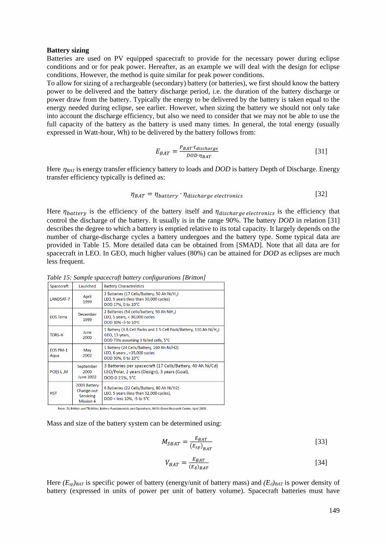
149
Battery sizing
Batteries are used on PV equipped spacecraft to provide for the necessary power during eclipse
conditions and or for peak power. Hereafter, as an example we will deal with the design for eclipse
conditions. However, the method is quite similar for peak power conditions.
To allow for sizing of a rechargeable (secondary) battery (or batteries), we first should know the battery
power to be delivered and the battery discharge period, i.e. the duration of the battery discharge or
power draw from the battery. Typically the energy to be delivered by the battery is taken equal to the
energy needed during eclipse, see earlier. However, when sizing the battery we should not only take
into account the discharge efficiency, but also we need to consider that we may not be able to use the
full capacity of the battery as the battery is used many times. In general, the total energy (usually
expressed in Watt-hour, Wh) to be delivered by the battery follows from:
𝐸𝐵𝐴𝑇 =𝑃𝐵𝐴𝑇∙𝑡𝑑𝑖𝑠𝑐ℎ𝑎𝑟𝑔𝑒
𝐷𝑂𝐷∙𝜂𝐵𝐴𝑇 [31]
Here BAT is energy transfer efficiency battery to loads and DOD is battery Depth of Discharge. Energy
transfer efficiency typically is defined as:
𝜂𝐵𝐴𝑇 = 𝜂𝑏𝑎𝑡𝑡𝑒𝑟𝑦 ∙ 𝜂𝑑𝑖𝑠𝑐ℎ𝑎𝑟𝑔𝑒 𝑒𝑙𝑒𝑐𝑡𝑟𝑜𝑛𝑖𝑐𝑠 [32]
Here 𝜂𝑏𝑎𝑡𝑡𝑒𝑟𝑦 is the efficiency of the battery itself and 𝜂𝑑𝑖𝑠𝑐ℎ𝑎𝑟𝑔𝑒 𝑒𝑙𝑒𝑐𝑡𝑟𝑜𝑛𝑖𝑐𝑠 is the efficiency that
control the discharge of the battery. It usually is in the range 90%. The battery DOD in relation [31]
describes the degree to which a battery is emptied relative to its total capacity. It largely depends on the
number of charge-discharge cycles a battery undergoes and the battery type. Some typical data are
provided in Table 15. More detailed data can be obtained from [SMAD]. Note that all data are for
spacecraft in LEO. In GEO, much higher values (80%) can be attained for DOD as eclipses are much
less frequent.
Table 15: Sample spacecraft battery configurations [Britton]
Mass and size of the battery system can be determined using:
𝑀𝑆𝐵𝐴𝑇 =𝐸𝐵𝐴𝑇
(𝐸𝑠𝑝)𝐵𝐴𝑇
[33]
𝑉𝐵𝐴𝑇 =𝐸𝐵𝐴𝑇
(𝐸𝛿)𝐵𝐴𝑇 [34]
Here (Esp)BAT is specific power of battery (energy/unit of battery mass) and (E)BAT is power density of
battery (expressed in units of power per unit of battery volume). Spacecraft batteries must have
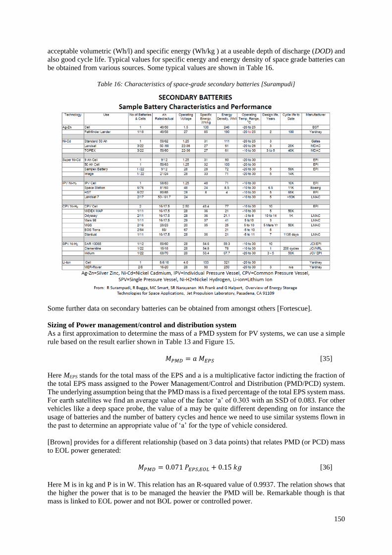
150
acceptable volumetric (Wh/l) and specific energy (Wh/kg ) at a useable depth of discharge (DOD) and
also good cycle life. Typical values for specific energy and energy density of space grade batteries can
be obtained from various sources. Some typical values are shown in Table 16.
Table 16: Characteristics of space-grade secondary batteries [Surampudi]
Some further data on secondary batteries can be obtained from amongst others [Fortescue].
Sizing of Power management/control and distribution system
As a first approximation to determine the mass of a PMD system for PV systems, we can use a simple
rule based on the result earlier shown in Table 13 and Figure 15.
𝑀𝑃𝑀𝐷 = 𝑎 𝑀𝐸𝑃𝑆 [35]
Here MEPS stands for the total mass of the EPS and a is a multiplicative factor indicting the fraction of
the total EPS mass assigned to the Power Management/Control and Distribution (PMD/PCD) system.
The underlying assumption being that the PMD mass is a fixed percentage of the total EPS system mass.
For earth satellites we find an average value of the factor ‘a’ of 0.303 with an SSD of 0.083. For other
vehicles like a deep space probe, the value of a may be quite different depending on for instance the
usage of batteries and the number of battery cycles and hence we need to use similar systems flown in
the past to determine an appropriate value of ‘a’ for the type of vehicle considered.
[Brown] provides for a different relationship (based on 3 data points) that relates PMD (or PCD) mass
to EOL power generated:
𝑀𝑃𝑀𝐷 = 0.071 𝑃𝐸𝑃𝑆,𝐸𝑂𝐿 + 0.15 𝑘𝑔 [36]
Here M is in kg and P is in W. This relation has an R-squared value of 0.9937. The relation shows that
the higher the power that is to be managed the heavier the PMD will be. Remarkable though is that
mass is linked to EOL power and not BOL power or controlled power.

151
To obtain further details of interest for the dimensioning and sizing of the PMD subsystem of the EPS,
it is useful to consider the main elements that make up the PMD subsystem. Main elements include:
• Power Conditioning Unit (PCU) which regulates the array power (array power regulator), the
charging of the batteries (battery charge regulator), the discharging of the batteries (battery
discharge regulator), see Figure 12. The PCU is a device that is computer controlled and hence
also has provisions that allow it to be commanded and to provide status (health) information to
the On-Board Computer (see later chapter on Command & Data Handling).
• Power Distribution Unit (PDU), which allows for distributing power to the payloads, heaters,
powered propulsion components, like valves, pyrotechnics for separation and deployment, etc.
• Power cabling, which transports the power from the source to the PCU and PCD and to the
various loads. Cables are to be shielded to reduce ElectroMagnetic Interference (EMI).
Sometimes the PCU and PDU are combined in a single Power Conditioning and Distribution Unit
(PCDU). Figure 16 shows examples of the mentioned PMD components.
Thales Next Generation PCU Therma small GEO PDU
Galileo S/C Therma PCDU S/C power cables
Figure 16: PMD components
For each of these components data can be collected and sizing rules determined. As a typical example,
some data have been collected in Table 17. From these data, we learn that mass and size of
PCU/PDU/PCDU relates strongly to the maximum controlled or distributed power according to:
𝑀𝑖 = 𝑃𝑖/𝑃𝑠𝑝,𝑖 [37]
𝑉𝑖 =𝑃𝑖
𝑃𝜌,𝑖 [38]
Here M is mass and V is volume, P is maximum controlled or distributed power, subscript i refers to
either PCU, PDU or PCDU. Psp is specific power and P is power density. It is noticed that controlled
or distributed power may be similar to array power, but may also be quite different as in peak power
conditions, the amount of power may rise above the power level provided by the array as also the battery
may deliver power. Using the tabulated data we find for the average specific power:

152
𝑃𝑠𝑝,𝑃𝐶𝑈 = 296 𝑊
𝑘𝑔(𝑆𝑆𝐷 = 76
𝑊
𝑘𝑔) [39]
𝑃𝑠𝑝,𝑃𝐷𝑈 = 71𝑊
𝑘𝑔(𝑆𝑆𝐷 = 14
𝑊
𝑘𝑔) [40]
𝑃𝑠𝑝,𝑃𝐶𝐷𝑈 = 145 𝑊
𝑘𝑔(𝑆𝑆𝐷 = 123
𝑊
𝑘𝑔) [41]
From these data follows that the PDU is relatively heavier than the PCU. The PCDU is somewhere in
between as it combines the two in a single device.
In above relations, also the sample standard deviation is given. For PCU this standard deviation is quite
high. This may be in part because data has not been interpreted correctly, but may also be related to
differences in PCU design. For instance, different types of array regulators may be used and sometimes
there is no battery charge or discharge regulator. In the work of [Brown] a similar relation for the mass
of the PCU can be found showing an average specific power of 0.0045 kg/kW. This nicely falls in the
range as indicated for the PCU specific power in the relation given in the current work. It may be argued
that the average specific power as given by Brown holds for larger PCU and hence may suggest that
specific mass depends on power level. However, this is considered out of scope and is left for the reader
to research for him/herself.
Table 17: PMD component design characteristics [various sources, see internet sources in reference list]
Type Provider Name of device Mass
[kg]
Maximum
controlled/distributed
power [kW]
Dimensions
[mm]
PCU Terma PCU 8.3 2.4 267x233x158
PCU Alcatel MHPCU 54.5 18 659x620x150
PCU MHPCU 44 12 563x620x150
PCU Terma Mars Express PCU 8.2 1.5 267x238x158
PCU XMM MRU 24 2.1 540x520x180
PCU Thales PCU <51 21.6
PCU Thales PCU <55 18
PCU Messenger PSE 6.5 1.6 286x196x142
PDU XMM SVM (service module) 16 1.4 455x270x200
PDU XMM FPA (payload module) 11 0.84 312x270x200
PDU XMM Pyro Regulator Unit 5.5 250x250x200
PDU XMM Mirror thermal control unit 15.8 1.005 402x274x220
PDU Terma PDU 13.2 1.000 425x285x160
PDU New Horizons PDU
PDU APL Messenger PDU 12.5 0.64 234x226x239
PCDU Terma Galileo PCDU 18.2 2.6 508x235x156
PCDU Surrey PCDU 4.4 0.2 670x305x39
PCDU Thales PCDU 4.5 330 W
PCDU Thales ARSAT PCDU 16.6 4.2 332x345x193
PCDU Thales ECRS PCDU 27.4 3.7 536x345x193
PCDU AAC Nano PCDU 0.045
PCDU ClydeS 3G EPS PCDU 0.086 0.034 95x90x15
PCDU Magellan PCDU 27 2 370x356x229
PCDU Magellan PCDU 12 0.5 370x180x229
* Magellan is Magellan Aerospace ; AAC is AAC Microtec, ClydeS is ClydeSpace
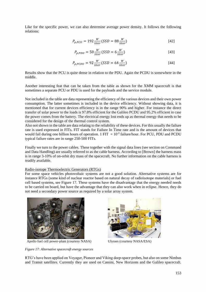
153
Like for the specific power, we can also determine average power density. It follows the following
relations:
𝑃𝜌,𝑃𝐶𝑈 = 192𝑊
𝑙𝑖𝑡𝑒𝑟(𝑆𝑆𝐷 = 88
𝑊
𝑙𝑖𝑡𝑒𝑟) [42]
𝑃𝜌,𝑃𝐷𝑈 = 50𝑊
𝑙𝑖𝑡𝑒𝑟(𝑆𝑆𝐷 = 6
𝑊
𝑙𝑖𝑡𝑒𝑟) [43]
𝑃𝜌,𝑃𝐶𝐷𝑈 = 92𝑊
𝑙𝑖𝑡𝑒𝑟(𝑆𝑆𝐷 = 64
𝑊
𝑙𝑖𝑡𝑒𝑟) [44]
Results show that the PCU is quite dense in relation to the PDU. Again the PCDU is somewhere in the
middle.
Another interesting feat that can be taken from the table as shown for the XMM spacecraft is that
sometimes a separate PCU or PDU is used for the payloads and the service module.
Not included in the table are data representing the efficiency of the various devices and their own power
consumption. The latter sometimes is included in the device efficiency. Without showing data, it is
mentioned that for current devices efficiency is in the range 90% and higher. For instance the direct
transfer of solar power to the loads is 97.8% efficient for the Galileo PCDU and 95.2% efficient in case
the power comes from the battery. The electrical energy lost ends up as thermal energy that needs to be
considered for the design of the thermal control system.
Also not shown in the table are data relating to the reliability of these devices. For this usually the failure
rate is used expressed in FITs. FIT stands for Failure In Time rate and is the amount of devices that
would fail during one billion hours of operation. 1 FIT = 10-9 failure/hour. For PCU, PDU and PCDU
typical failure rates are in range 250-500 FITs.
Finally we turn to the power cables. These together with the signal data lines (see section on Command
and Data Handling) are usually referred to as the cable harness. According to [Brown] the harness mass
is in range 3-10% of on-orbit dry mass of the spacecraft. No further information on the cable harness is
readily available.
Radio-isotope Thermoelectric Generators (RTGs)
For some space vehicles photovoltaic systems are not a good solution. Alternative systems are for
instance RTGs (some kind of nuclear reactor based on natural decay of radioisotope materials) or fuel
cell based systems, see Figure 17. These systems have the disadvantage that the energy needed needs
to be carried on board, but have the advantage that they can also work when in eclipse. Hence, they do
not need a secondary power source as required by a solar array system.
Apollo fuel cell power-plant (courtesy NASA) Ulysses (courtesy NASA/ESA)
Figure 17: Alternative spacecraft energy sources
RTG’s have been applied on Voyager, Pioneer and Viking deep-space probes, but also on some Nimbus
and Transit satellites. Currently they are used on Cassini, New Horizons and the Galileo spacecraft.

154
First US RTGs, developed under the US SNAP (Systems for Nuclear Auxiliary Power) program,
produced about 2.7 watts of electric power. The most recently designed system, the General Purpose
Heat Source RTG (GPHS-RTG), generates about 290 watts of electric power at BOL and 250 W at
EOL. It weighs about 55 kg of which about 11 kg is fuel (about 7.5 kg of isotope fuel, remainder is
impurities). Thermal power is 4234 W.
Sizing of RTGs is usually on peak power to be delivered as usually no storage system is included in the
system. Another factor that should be taken into account is that because of natural decay the amount of
radioactive isotope in the reactor reduces and hence the power delivery reduces with increasing
operation time. For power P at time t follows:
𝑃 = 𝑃𝑜 ∙ 𝑒(
−0.693
𝜏1 2⁄𝑡)
[45]
Here P0 is initial power, and 1/2 is "half-life" (the time it takes for P to be 1/2 of Po). From [Fortescue]
the following data for some isotope fuels is obtained:
Cost figures are based on FY 1999 cost.
Note that cost figures in the table are given per Watt of thermal power. In practice, only a few percent
of thermal power produced is converted to electric power. The remainder is converted to heat, which is
to be radiated away. This is why the Ulysses RTG is painted black and has cooling fins.
For a derivation of the RTG power relation (equation [45]), it is considered that the power produced
decreases at a rate proportional to its value (linear decay model):
𝑑𝑃 𝑑𝑡⁄ = −𝛼𝑃 => Separation of variables => 𝑑𝑃
𝑃= −𝛼𝑑𝑡
Integration gives 𝑙𝑛(𝑃 𝑃𝑜⁄ ) = −𝛼𝑡 with Po is available power at time t = 0. After rearranging we
obtain 𝑃 = 𝑃𝑜 ∙ 𝑒(−𝛼𝑡). Next, using the information that at half-life the available power has reduced
with a factor 0.5, it follows: 𝑃 = 1 2⁄ 𝑃𝑜 ∙ 𝑒(−𝛼𝜏0.5). This gives −𝛼𝜏0.5 = ln(1 2⁄ ) = −0.693 and we
obtain: 𝛼 = 0.693 𝜏0.5⁄ . Substitution of the relation for the half time in the relation for P (𝑃 = 𝑃𝑜 ∙
𝑒(−𝛼𝑡)) results in [45].
Once the BOL power is determined, the mass of an RTG system can be estimated using:
𝑀𝑅𝑇𝐺 =𝑃𝑜
(𝑃𝑠𝑝)𝑅𝑇𝐺
[46]
Here (Psp)RTG = RTG specific power (typically in units of We/kg) and Po is initial RTG power (power at
Begin Of Life, BOL). Typical values of RTG specific power can be obtained from literature. To this
mass, we should then still add the mass of an accompanying power management and distribution system.
As a starting point, we may use the relations as discussed earlier for the PMD of photovoltaic systems.
However, we may need to look for more specific data as the PCU for a radio-isotope system does not
require an array regulator. Also a battery charge and discharge regulator is not always needed.
Table 18: Characteristic data of some radio-isotope fuels
155
Fuel cell systems
Fuel cell systems have been used on the Gemini spacecraft and the Apollo service module. More
recently they have been used on the Space Shuttle. The Apollo fuel cell system consists of three 31-cell
hydrogen oxygen fuel cell stacks which provide 28 volts, two cryogenic oxygen and two cryogenic
hydrogen tanks. The Space Shuttle operates 3 fuel cell power-plants, each supplying its own isolated,
simultaneously operating 28-volt dc bus. The power-plant section of each system consists of 96 cells
contained in three sub-stacks.
Dimensioning parameters for a fuel cell system are peak power level and total energy need. Both should
be known at the start of the design for fuel cell systems. As one aims to keep the required power output
of a fuel cell steady, this means that excess power must be shunted away in the form of heat. This should
be taken into account when designing the thermal system of a spacecraft.
To estimate the mass of a fuel cell system a very first approach is to consider the system as consisting
of two elements, being the dry fuel cell system, consisting of the fuel cell power-plant, the feed system
and the controls, and the reactants. Notice that for now the reactant storage system is not included, see
later in this section.
𝑀𝑓𝑢𝑒𝑙 𝑐𝑒𝑙𝑙 𝑠𝑦𝑠𝑡𝑒𝑚 = (𝑀𝑓𝑢𝑒𝑙 𝑐𝑒𝑙𝑙 𝑠𝑦𝑠𝑡𝑒𝑚)𝑑𝑟𝑦
+ 𝑀𝑟𝑒𝑎𝑐𝑡𝑎𝑛𝑡𝑠 + 𝑀𝑠𝑡𝑜𝑟𝑎𝑔𝑒 [47]
Of these, the dry fuel cell system mass is estimated based on the (maximum) power output (P) to be
generated by the system and the fuel cell system specific power (Psp)fc according to:
(𝑀𝑓𝑢𝑒𝑙 𝑐𝑒𝑙𝑙 𝑠𝑦𝑠𝑡𝑒𝑚)𝑑𝑟𝑦
=𝑃
(𝑃𝑠𝑝)𝑓𝑐
[48]
Reactant mass is estimated based on the total energy (E) to be delivered by the fuel cell system and
the reactant consumption rate (Crate):
𝑀𝑟𝑒𝑎𝑐𝑡𝑎𝑛𝑡𝑠 = 𝐸 ∙ 𝐶𝑟𝑎𝑡𝑒 [49]
From [Fortescue] Tables 10.3 and 10.5, it is found that the specific power of a fuel cell power-plant
(excluding tankage) is in the range 25-300 We/kg, where the higher values apply to more modern fuel
cell systems. Typical fuel cell mass density (based on Space Shuttle fuel cell system) is about 750 kg/m3.
Next to the system itself, we must also to take into account the reactants needed to provide for the
required energy. For instance, for a hydrogen-oxygen fuel cell hydrogen-oxygen consumption (mass
ratio 1 kg of hydrogen reacts with 8 kg of hydrogen) rate typically is ~0.5 kg/kWh.
Example: Sizing of fuel cell system
Consider a fuel cell system that is required to deliver 3360 kWh at an average power level of 10 kW
(operational life of 336 hours or 14 days). It follows for the mass of the fuel cell:
Mfc = P/Psp = 10000 (Watt) / 100 (Watt/kg) = 100 kg
Here the specific power of fuel cell power-plant is taken equal to 100 W/kg. For the mass of the reactants
follows:
3360(kWh) x 0.5(kg/kWh) = 1680 kg and includes about 186.5 kg of hydrogen and 1493.5 kg of oxygen.
How to determine the mass and volume of the reactant storage system is dealt with in the lecture material
on launch vehicle design, but is highly linked to the volume of the cryogenic oxygen and hydrogen.
Mass density of these species can be obtained from the propulsion section, see later in this work.
Next to the fuel cell system itself, we also should consider an accompanying power management and
distribution system. As a starting point for the mass and size estimation of PMD components, we may
use the relations as discussed earlier for the PMD of photovoltaic systems. However, as fuel cell systems
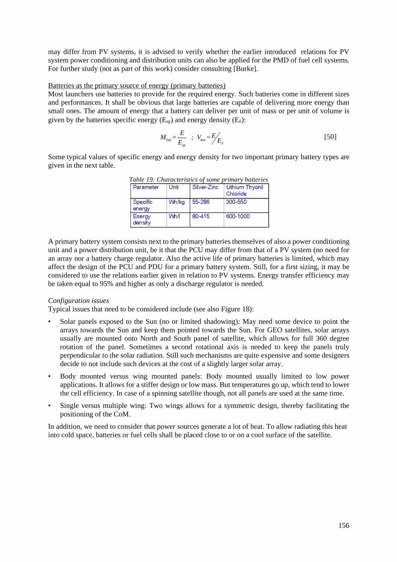
156
may differ from PV systems, it is advised to verify whether the earlier introduced relations for PV
system power conditioning and distribution units can also be applied for the PMD of fuel cell systems.
For further study (not as part of this work) consider consulting [Burke].
Batteries as the primary source of energy (primary batteries)
Most launchers use batteries to provide for the required energy. Such batteries come in different sizes
and performances. It shall be obvious that large batteries are capable of delivering more energy than
small ones. The amount of energy that a battery can deliver per unit of mass or per unit of volume is
given by the batteries specific energy (Esp) and energy density (E):
bat bat
δsp
E EM = ; V =EE
[50]
Some typical values of specific energy and energy density for two important primary battery types are
given in the next table.
Table 19: Characteristics of some primary batteries
A primary battery system consists next to the primary batteries themselves of also a power conditioning
unit and a power distribution unit, be it that the PCU may differ from that of a PV system (no need for
an array nor a battery charge regulator. Also the active life of primary batteries is limited, which may
affect the design of the PCU and PDU for a primary battery system. Still, for a first sizing, it may be
considered to use the relations earlier given in relation to PV systems. Energy transfer efficiency may
be taken equal to 95% and higher as only a discharge regulator is needed.
Configuration issues
Typical issues that need to be considered include (see also Figure 18):
• Solar panels exposed to the Sun (no or limited shadowing): May need some device to point the
arrays towards the Sun and keep them pointed towards the Sun. For GEO satellites, solar arrays
usually are mounted onto North and South panel of satellite, which allows for full 360 degree
rotation of the panel. Sometimes a second rotational axis is needed to keep the panels truly
perpendicular to the solar radiation. Still such mechanisms are quite expensive and some designers
decide to not include such devices at the cost of a slightly larger solar array.
• Body mounted versus wing mounted panels: Body mounted usually limited to low power
applications. It allows for a stiffer design or low mass. But temperatures go up, which tend to lower
the cell efficiency. In case of a spinning satellite though, not all panels are used at the same time.
• Single versus multiple wing: Two wings allows for a symmetric design, thereby facilitating the
positioning of the CoM.
In addition, we need to consider that power sources generate a lot of heat. To allow radiating this heat
into cold space, batteries or fuel cells shall be placed close to or on a cool surface of the satellite.
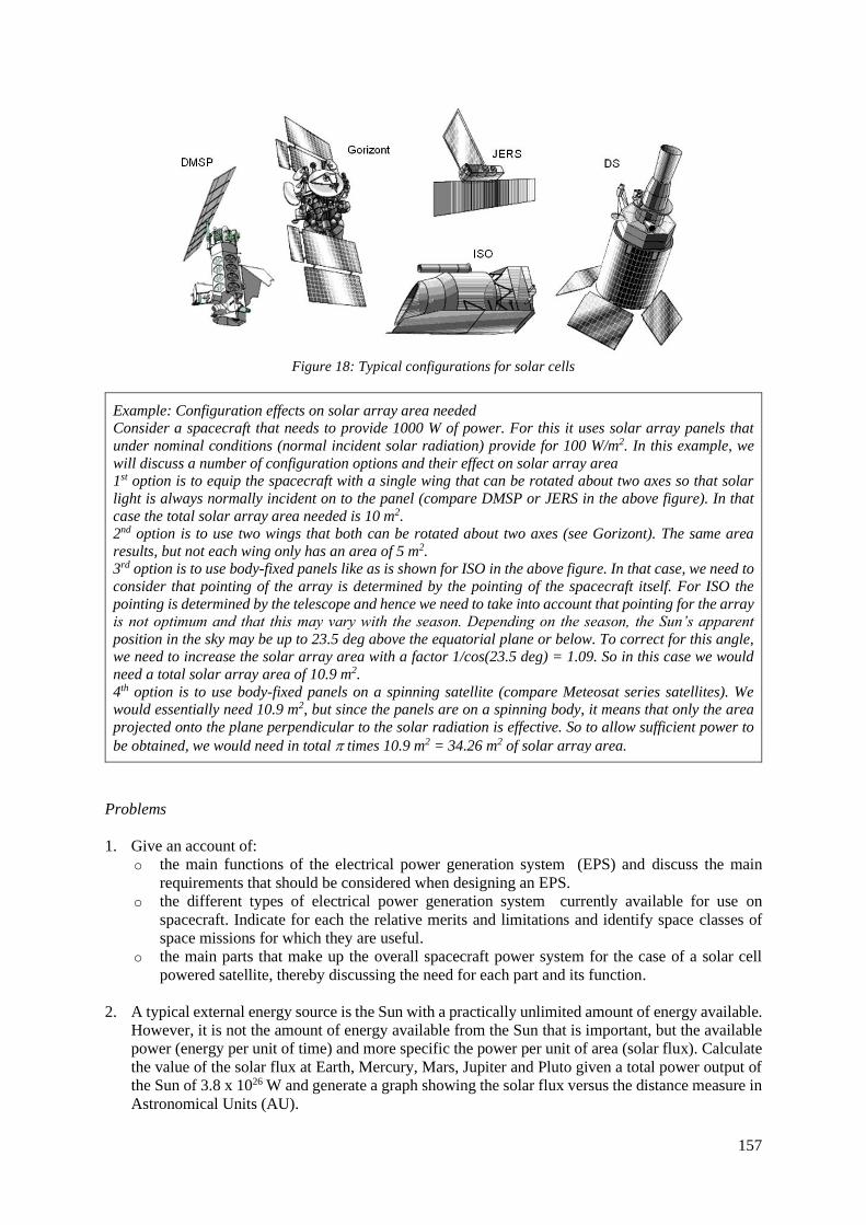
157
Figure 18: Typical configurations for solar cells
Example: Configuration effects on solar array area needed Consider a spacecraft that needs to provide 1000 W of power. For this it uses solar array panels that
under nominal conditions (normal incident solar radiation) provide for 100 W/m2. In this example, we
will discuss a number of configuration options and their effect on solar array area 1st option is to equip the spacecraft with a single wing that can be rotated about two axes so that solar
light is always normally incident on to the panel (compare DMSP or JERS in the above figure). In that
case the total solar array area needed is 10 m2. 2nd option is to use two wings that both can be rotated about two axes (see Gorizont). The same area
results, but not each wing only has an area of 5 m2. 3rd option is to use body-fixed panels like as is shown for ISO in the above figure. In that case, we need to
consider that pointing of the array is determined by the pointing of the spacecraft itself. For ISO the
pointing is determined by the telescope and hence we need to take into account that pointing for the array is not optimum and that this may vary with the season. Depending on the season, the Sun’s apparent
position in the sky may be up to 23.5 deg above the equatorial plane or below. To correct for this angle, we need to increase the solar array area with a factor 1/cos(23.5 deg) = 1.09. So in this case we would
need a total solar array area of 10.9 m2.
4th option is to use body-fixed panels on a spinning satellite (compare Meteosat series satellites). We would essentially need 10.9 m2, but since the panels are on a spinning body, it means that only the area
projected onto the plane perpendicular to the solar radiation is effective. So to allow sufficient power to
be obtained, we would need in total times 10.9 m2 = 34.26 m2 of solar array area.
Problems
1. Give an account of:
o the main functions of the electrical power generation system (EPS) and discuss the main
requirements that should be considered when designing an EPS.
o the different types of electrical power generation system currently available for use on
spacecraft. Indicate for each the relative merits and limitations and identify space classes of
space missions for which they are useful.
o the main parts that make up the overall spacecraft power system for the case of a solar cell
powered satellite, thereby discussing the need for each part and its function.
2. A typical external energy source is the Sun with a practically unlimited amount of energy available.
However, it is not the amount of energy available from the Sun that is important, but the available
power (energy per unit of time) and more specific the power per unit of area (solar flux). Calculate
the value of the solar flux at Earth, Mercury, Mars, Jupiter and Pluto given a total power output of
the Sun of 3.8 x 1026 W and generate a graph showing the solar flux versus the distance measure in
Astronomical Units (AU).

158
3. You are designing the EPS for a spacecraft. The EPS is required to deliver an average 100 W of
power for a period of 1 week. Which type of EPS do you consider the most likely candidate for this
mission and why?
Answer: A fuel cell system is the most likely EPS candidate. The reason is that this system has an
internal energy source and hence can work independently from the environment, while mass
remains within reasonable amounts (lower than for a battery system). An RTG might also be a
possibility, but this adds a radiation problem. Also fuel for RTGs is not abundant, so if an
alternative is available, it is better to use the alternative.
4. You are designing a deep space probe. This space probe is to carry a payload requiring 50 W of
power. Using data from historical spacecraft you have determined the following regression
relationship between on board generated power and payload power, both in Watt:
Pgenerated = 209.2 ln(Ppayload) - 491.8 W
This relation has an RSE of 23%. Determine for this vehicle the range that should be taken into
account for the on-board generated power given that this range should encompass 95% of all
possible outcomes.
Answer:176 - 477 W (nominal power at 50 W = 326.6 W; RSE = 0.23 x 326.6 W = 75.1 W)
5. A spacecraft in orbit about Mars requires a stable 200 W for operations. You consider using a PV
array for power provision. Given are:
o Orbital period: 3 hour
o Eclipse period: 58 min
o Path efficiency during daytime: 80%
o Path efficiency during eclipse: 60%
Determine power that needs to be provided for by the solar array
Answer: 408 W
6. The end-of-mission life capability of a spacecraft power system is 200 watts. Your instrument is
expected to use 50 watts, including 25% contingency. You are allotted 75 watts by the satellite
provider.
a) What is the instrument’s contingency
b) What is the power margin in watts and as a percentage (%)?
Answers: a) 12.5 W, b) Power margin is 75 W-50 W = 25 W; (75 W-50 W)/75W x 100% = 33.33%
7. A cubical S/C in LEO is equipped with a PV array to provide 400 W. Given is a linear dimension
of the vehicle of 2 m and a power density of the array of 100 W/m2.
A. Consider the array area needed in case we have a 3-axis stabilized craft that allows keeping one
side of the craft perpendicular to the incoming solar radiation
B. Same question, but now in case the craft is spin stabilized with spin axis perpendicular to the
incoming solar radiation
Answers: A) 4 m2; B) 12.6 m2
8. A solar array in space is producing 3.5 kW at Begin Of Life (BOL). Over its life this power reduces
because of degradation due to radiation. Given is that the power output of the array reduces with
3%/year and that the life of the array is 15.6 year.
Array power delivered by the solar array of the spacecraft at end of Life (EOL) is …?

159
Answer: 2.19 kW
9. A battery system is selected to provide 620 W of power for a period of 35 minutes. Due to the cyclic
use of the battery, the battery is only capable of using 12% of its capacity. In addition, because of
high discharge rates the battery is only 80% efficient. Given that the specific energy of the battery
selected is 35 Wh/kg and the specific energy density 100 Wh/l, calculate for the battery system:
A. Battery storage capacity (in Wh)
B. Total battery mass, and
C. Total battery volume
Answer: A) 3800 Wh, B) 107 kg, C) 381 liter.
10. You have designed an RTG using an isotope fuel with a half-life of 45 days to provide 1000 W at
start of mission. End of mission is after 1 year. What is for this RTG the available power at end
of mission?
A. 500 W
B. 123.3 W
C. 3.62 W
D. 12.33 W
Answer: C is correct answer.
11. The following RTG data are taken from [Wikipedia]:
Average specific power of RTG system is ... ?
Answer: Average specific power value is 3.04 W/kg with an SSD of 1.26 W/kg.
More problems for exercising upon are available via the course web pages (look for Mobius exercises)
or in the tutorial material.
160
7. Launcher design 7.1 The rocket equation The rocket- or Tsiolkowsky equation can be written as:
ln ; / = = initialinitial final
final
MV w M M
M [51]
It essentially relates the velocity change V that can be realized by a rocket propelled vehicle to its
initial and final mass (M) and some effective velocity (w) with which the (rocket) propellants are
expelled. The latter hence is also referred to as effective rocket exhaust velocity or shortly effective
exhaust velocity. The ratio of initial to final vehicle mass, here denoted by , is referred to as the vehicle
mass ratio while the inverse of this ratio is referred to as vehicle inert mass fraction (a value smaller
than one). A derivation of the rocket equation can be found in AE1110-II. In this course it was also
introduced a relation between the specific impulse (Isp), i.e. the total impulse delivered by the rocket per
unit of propellant weight, and the effective exhaust velocity:
0= spw I g [52]
Here go is Earth gravitational acceleration at sea level. Both specific impulse and the exhaust velocity
depend on the type of rocket propulsion selected. This will be explained later in more detail. Another
aspect introduced in AE1110-II is that with varying altitude the exhaust velocity, and hence also the
specific impulse, of a rocket tends to change. This is related to the change in atmospheric pressure with
altitude. As an example, it is mentioned that at sea level (high atmospheric pressure) the Space Shuttle
Solid Rocket Booster produces an Isp of 242 s and in vacuum (absence of atmosphere) 268.6 s. We write
Isp,sealevel = 242 s and Isp,vacuum = 268.6 s. For the V2 rocket, these values are 270 s at sea level and 312 s
in vacuum. The difference between the values for the Space Shuttle and the V2 can be explained from
the use of different propellants, which will be highlighted later in this course in more detail, and from
differences in engine design. The latter will be dealt with later in the curriculum.
Notice that the effective exhaust velocity of the Space Shuttle rocket booster varies from about 2375
m/s (242 s x 9.81 m/s2) at sea level to 2635 m/s in vacuum. For the V2 rocket these values are 2650 and
3060 m/s, respectively.
Because of the specific impulse (and hence also the effective exhaust velocity) changing with altitude,
we use an average value over the burn/action time of the rocket to obtain a “mission average” value:
0 0
0
0 0
0 0
= = =
b b
b b
t t
sp t t
T dt m w dtw
Ig
m g dt m g dt
[53]
Here T and w are instantaneous rocket thrust and effective exhaust velocity, respectively and m is
propellant mass flow rate. Notice that if a rocket stays at constant altitude, both specific impulse and
exhaust velocity remain constant unless we change the settings of the rocket motor. The latter will be
dealt with in later courses.
Next figure shows some results obtained from the rocket equation. It shows the velocity change as a
function of rocket mass ratio for two different (effective) exhaust velocities.
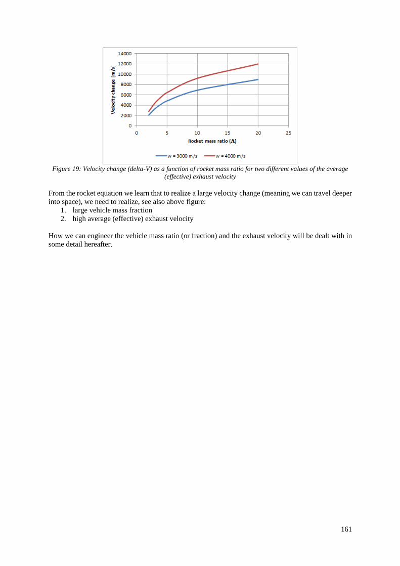
161
Figure 19: Velocity change (delta-V) as a function of rocket mass ratio for two different values of the average
(effective) exhaust velocity
From the rocket equation we learn that to realize a large velocity change (meaning we can travel deeper
into space), we need to realize, see also above figure:
1. large vehicle mass fraction
2. high average (effective) exhaust velocity
How we can engineer the vehicle mass ratio (or fraction) and the exhaust velocity will be dealt with in
some detail hereafter.

162
7.2 Single stage rockets Next figure shows a typical layout of a single stage rocket. It essentially
consists of a rocket stage and a payload (also referred to as useful load) with
a nose cone on top. For reasons of simplicity, we consider the rocket stage
to consist of (usable) propellant and structure (everything else, including
engines, stabilization fins, tanks, piping, and aerodynamic control surfaces).
For this rocket, we can write the initial (at start of the propelled phase) and
final (or empty) mass (at end of propelled phase) of the rocket as:
𝑀𝑖𝑛𝑖𝑡𝑖𝑎𝑙 = 𝑀𝑜 = 𝑀𝑢 + 𝑀𝑠 + 𝑀𝑝
𝑀𝑓𝑖𝑛𝑎𝑙 = 𝑀𝑓 = 𝑀𝑢 + 𝑀𝑠
[54]
Here Mu is mass of useful load (payload) including the mass of the nose
cone, Ms is structural mass of rocket stage and Mp is propellant mass carried
on board of the stage.
Rocket propellant mass then follows from:
Mpropellant = Mp = Mo - Mf [55]
Earlier we found that to attain a high delta-V, the mass ratio as defined in relation [2] needs to be
maximized.
Using above relations in combination with the rocket equation, it can easily be found that to attain a
high mass ratio (for a given payload mass) and hence maximizing the propellant mass the structural
mass should be minimized.
Taking the relation for initial mass and dividing both sides by Mo, we obtain:
1 =𝑀𝑢
𝑀𝑜+
𝑀𝑠
𝑀𝑜+
𝑀𝑝
𝑀𝑜 [56]
The first ratio is the vehicle payload fraction (𝑓𝑢 = ) as defined earlier, the second is the vehicle
structural mass fraction (𝑓𝑠) and the third one is the vehicle propellant mass fraction (𝑓𝑝). It follows that
all three fractions have a value smaller than 1.
A further useful mass fraction is the stage structural coefficient (sometimes also referred to as stage
structural efficiency) . This is defined as the ratio of stage structural mass divided by the stage
propellant mass:
𝜎 =𝑀𝑠
𝑀𝑝 [57]
A low value of this coefficient indicates that little structural mass is needed to store a certain amount of
propellant. Hence this indicates an efficient design. It is actually the technology selected for the stage
design that determines the value of the structural coefficient.
Figure 20: Basic lay-out of
single stage rocket
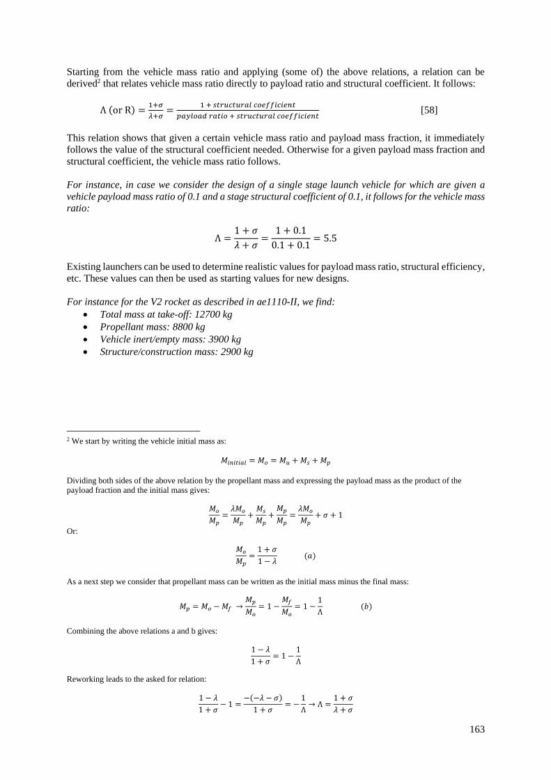
163
Starting from the vehicle mass ratio and applying (some of) the above relations, a relation can be
derived2 that relates vehicle mass ratio directly to payload ratio and structural coefficient. It follows:
Λ (or R) =1+𝜎
𝜆+𝜎=
1 + 𝑠𝑡𝑟𝑢𝑐𝑡𝑢𝑟𝑎𝑙 𝑐𝑜𝑒𝑓𝑓𝑖𝑐𝑖𝑒𝑛𝑡
𝑝𝑎𝑦𝑙𝑜𝑎𝑑 𝑟𝑎𝑡𝑖𝑜 + 𝑠𝑡𝑟𝑢𝑐𝑡𝑢𝑟𝑎𝑙 𝑐𝑜𝑒𝑓𝑓𝑖𝑐𝑖𝑒𝑛𝑡 [58]
This relation shows that given a certain vehicle mass ratio and payload mass fraction, it immediately
follows the value of the structural coefficient needed. Otherwise for a given payload mass fraction and
structural coefficient, the vehicle mass ratio follows.
For instance, in case we consider the design of a single stage launch vehicle for which are given a
vehicle payload mass ratio of 0.1 and a stage structural coefficient of 0.1, it follows for the vehicle mass
ratio:
Λ =1 + 𝜎
𝜆 + 𝜎=
1 + 0.1
0.1 + 0.1= 5.5
Existing launchers can be used to determine realistic values for payload mass ratio, structural efficiency,
etc. These values can then be used as starting values for new designs.
For instance for the V2 rocket as described in ae1110-II, we find:
• Total mass at take-off: 12700 kg
• Propellant mass: 8800 kg
• Vehicle inert/empty mass: 3900 kg
• Structure/construction mass: 2900 kg
2 We start by writing the vehicle initial mass as:
𝑀𝑖𝑛𝑖𝑡𝑖𝑎𝑙 = 𝑀𝑜 = 𝑀𝑢 + 𝑀𝑠 + 𝑀𝑝
Dividing both sides of the above relation by the propellant mass and expressing the payload mass as the product of the
payload fraction and the initial mass gives:
𝑀𝑜
𝑀𝑝=
𝜆𝑀𝑜
𝑀𝑝+
𝑀𝑠
𝑀𝑝+
𝑀𝑝
𝑀𝑝=
𝜆𝑀𝑜
𝑀𝑝+ 𝜎 + 1
Or:
𝑀𝑜
𝑀𝑝=
1 + 𝜎
1 − 𝜆 (𝑎)
As a next step we consider that propellant mass can be written as the initial mass minus the final mass:
𝑀𝑝 = 𝑀𝑜 − 𝑀𝑓 →𝑀𝑝
𝑀𝑜= 1 −
𝑀𝑓
𝑀𝑜= 1 −
1
Λ (𝑏)
Combining the above relations a and b gives:
1 − 𝜆
1 + 𝜎= 1 −
1
Λ
Reworking leads to the asked for relation:
1 − 𝜆
1 + 𝜎− 1 =
−(−𝜆 − 𝜎)
1 + 𝜎= −
1
Λ→ Λ =
1 + 𝜎
𝜆 + 𝜎
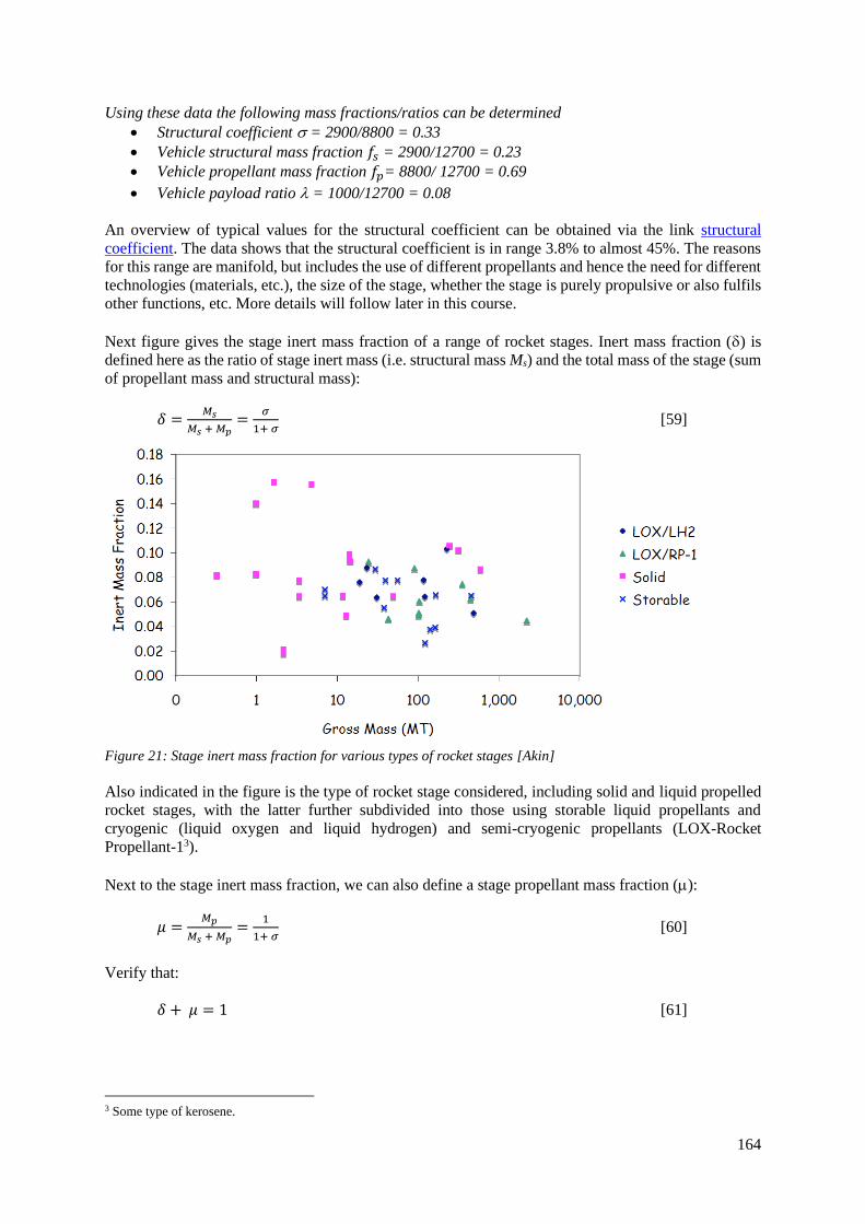
164
Using these data the following mass fractions/ratios can be determined
• Structural coefficient = 2900/8800 = 0.33
• Vehicle structural mass fraction 𝑓𝑠 = 2900/12700 = 0.23
• Vehicle propellant mass fraction 𝑓𝑝= 8800/ 12700 = 0.69
• Vehicle payload ratio = 1000/12700 = 0.08
An overview of typical values for the structural coefficient can be obtained via the link structural
coefficient. The data shows that the structural coefficient is in range 3.8% to almost 45%. The reasons
for this range are manifold, but includes the use of different propellants and hence the need for different
technologies (materials, etc.), the size of the stage, whether the stage is purely propulsive or also fulfils
other functions, etc. More details will follow later in this course.
Next figure gives the stage inert mass fraction of a range of rocket stages. Inert mass fraction () is
defined here as the ratio of stage inert mass (i.e. structural mass Ms) and the total mass of the stage (sum
of propellant mass and structural mass):
𝛿 =𝑀𝑠
𝑀𝑠 + 𝑀𝑝=
𝜎
1+ 𝜎 [59]
Figure 21: Stage inert mass fraction for various types of rocket stages [Akin]
Also indicated in the figure is the type of rocket stage considered, including solid and liquid propelled
rocket stages, with the latter further subdivided into those using storable liquid propellants and
cryogenic (liquid oxygen and liquid hydrogen) and semi-cryogenic propellants (LOX-Rocket
Propellant-13).
Next to the stage inert mass fraction, we can also define a stage propellant mass fraction ():
𝜇 =𝑀𝑝
𝑀𝑠 + 𝑀𝑝=
1
1+ 𝜎 [60]
Verify that:
𝛿 + 𝜇 = 1 [61]
3 Some type of kerosene.
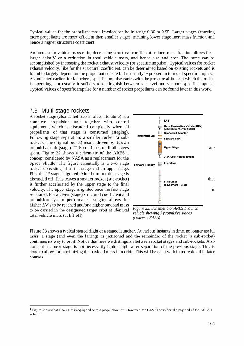
165
Typical values for the propellant mass fraction can be in range 0.80 to 0.95. Larger stages (carrying
more propellant) are more efficient than smaller stages, meaning lower stage inert mass fraction and
hence a higher structural coefficient.
An increase in vehicle mass ratio, decreasing structural coefficient or inert mass fraction allows for a
larger delta-V or a reduction in total vehicle mass, and hence size and cost. The same can be
accomplished by increasing the rocket exhaust velocity (or specific impulse). Typical values for rocket
exhaust velocity, like for the structural coefficient, can be determined based on existing rockets and is
found to largely depend on the propellant selected. It is usually expressed in terms of specific impulse.
As indicated earlier, for launchers, specific impulse varies with the pressure altitude at which the rocket
is operating, but usually it suffices to distinguish between sea level and vacuum specific impulse.
Typical values of specific impulse for a number of rocket propellants can be found later in this work.
7.3 Multi-stage rockets A rocket stage (also called step in older literature) is a
complete propulsion unit together with control
equipment, which is discarded completely when all
propellants of that stage is consumed (staging).
Following stage separation, a smaller rocket (a sub-
rocket of the original rocket) results driven by its own
propulsive unit (stage). This continues until all stages are
spent. Figure 22 shows a schematic of the ARES 1
concept considered by NASA as a replacement for the
Space Shuttle. The figure essentially is a two stage
rocket4 consisting of a first stage and an upper stage.
First the 1st stage is ignited. After burn-out this stage is
discarded off. This leaves a smaller rocket (sub-rocket) that
is further accelerated by the upper stage to the final
velocity. The upper stage is ignited once the first stage is
separated. For a given (stage) structural coefficient and
propulsion system performance, staging allows for
higher ΔV’s to be reached and/or a higher payload mass
to be carried in the designated target orbit at identical
total vehicle mass (at lift-off).
Figure 23 shows a typical staged flight of a staged launcher. At various instants in time, no longer useful
mass, a stage (and even the fairing), is jettisoned and the remainder of the rocket (a sub-rocket)
continues its way to orbit. Notice that here we distinguish between rocket stages and sub-rockets. Also
notice that a next stage is not necessarily ignited right after separation of the previous stage. This is
done to allow for maximizing the payload mass into orbit. This will be dealt with in more detail in later
courses.
4 Figure shows that also CEV is equipped with a propulsion unit. However, the CEV is considered a payload of the ARES 1
vehicle.
Figure 22: Schematic of ARES 1 launch
vehicle showing 3 propulsive stages
(courtesy NASA)
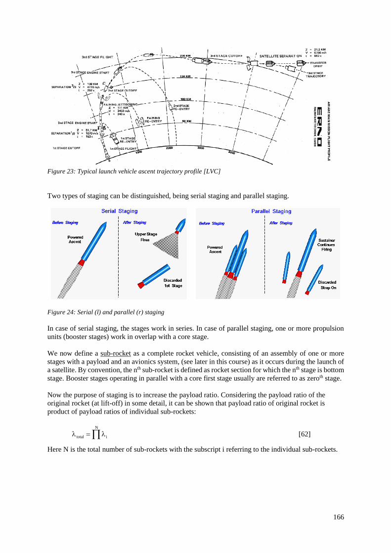
166
Figure 23: Typical launch vehicle ascent trajectory profile [LVC]
Two types of staging can be distinguished, being serial staging and parallel staging.
Figure 24: Serial (l) and parallel (r) staging
In case of serial staging, the stages work in series. In case of parallel staging, one or more propulsion
units (booster stages) work in overlap with a core stage.
We now define a sub-rocket as a complete rocket vehicle, consisting of an assembly of one or more
stages with a payload and an avionics system, (see later in this course) as it occurs during the launch of
a satellite. By convention, the nth sub-rocket is defined as rocket section for which the nth stage is bottom
stage. Booster stages operating in parallel with a core first stage usually are referred to as zeroth stage.
Now the purpose of staging is to increase the payload ratio. Considering the payload ratio of the
original rocket (at lift-off) in some detail, it can be shown that payload ratio of original rocket is
product of payload ratios of individual sub-rockets:
N
total i = [62]
Here N is the total number of sub-rockets with the subscript i referring to the individual sub-rockets.
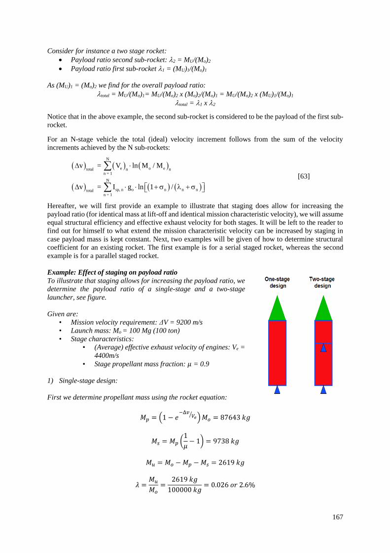
167
Consider for instance a two stage rocket:
• Payload ratio second sub-rocket: 2 = MU/(Mo)2
• Payload ratio first sub-rocket 1 = (MU)1/(Mo)1
As (MU)1 = (Mo)2 we find for the overall payload ratio:
total = MU/(Mo)1= MU/(Mo)2 x (Mo)2/(Mo)1 = MU/(Mo)2 x (MU)1/(Mo)1
total = 1 x 2
Notice that in the above example, the second sub-rocket is considered to be the payload of the first sub-
rocket.
For an N-stage vehicle the total (ideal) velocity increment follows from the sum of the velocity
increments achieved by the N sub-rockets:
( ) ( ) ( )
( ) ( ) ( )
N
e o etotal n nn = 1
N
sp, n o n n ntotaln = 1
v = V ln M / M
v = I g ln 1 /
+ +
[63]
Hereafter, we will first provide an example to illustrate that staging does allow for increasing the
payload ratio (for identical mass at lift-off and identical mission characteristic velocity), we will assume
equal structural efficiency and effective exhaust velocity for both stages. It will be left to the reader to
find out for himself to what extend the mission characteristic velocity can be increased by staging in
case payload mass is kept constant. Next, two examples will be given of how to determine structural
coefficient for an existing rocket. The first example is for a serial staged rocket, whereas the second
example is for a parallel staged rocket.
Example: Effect of staging on payload ratio
To illustrate that staging allows for increasing the payload ratio, we
determine the payload ratio of a single-stage and a two-stage
launcher, see figure.
Given are:
• Mission velocity requirement: ΔV = 9200 m/s
• Launch mass: Mo = 100 Mg (100 ton)
• Stage characteristics:
• (Average) effective exhaust velocity of engines: Ve =
4400m/s
• Stage propellant mass fraction: 𝜇 = 0.9
1) Single-stage design:
First we determine propellant mass using the rocket equation:
𝑀𝑝 = (1 − 𝑒−Δ𝑣
𝑉𝑒⁄
) 𝑀𝑜 = 87643 𝑘𝑔
𝑀𝑠 = 𝑀𝑝 (1
𝜇− 1) = 9738 𝑘𝑔
𝑀𝑢 = 𝑀𝑜 − 𝑀𝑝 − 𝑀𝑠 = 2619 𝑘𝑔
𝜆 =𝑀𝑢
𝑀𝑜=
2619 𝑘𝑔
100000 𝑘𝑔= 0.026 𝑜𝑟 2.6%

168
2) Two-stage design:
For the design of the serial staged two-stage rocket, we assume that the total mission delta-V is divided
equally over the two stages (sub-rockets) and that both stages have a propellant mass fraction of 0.9.
It follows:
For the propellant mass of the first sub-rocket:
𝑀𝑝,1 = (1 − 𝑒−Δ𝑣1
𝑉𝑒,1⁄
) 𝑀𝑜,1 = 64847 𝑘𝑔
The structural mass of stage 1 is:
𝑀𝑠,1 = 𝑀𝑝,1 (1
𝜇1− 1) = 72015 𝑘𝑔
This leaves for the useful load of the first sub-rocket:
𝑀𝑢,1 = 𝑀𝑜,2 = 𝑀𝑜,1 − 𝑀𝑝,1 − 𝑀𝑠,1 = 27948 𝑘𝑔
For the propellant mass of the second sub-rocket follows:
𝑀𝑝,2 = (1 − 𝑒−Δ𝑣2
𝑉𝑒,2⁄
) 𝑀𝑜,2 = 18123 𝑘𝑔
The structural mass is:
𝑀𝑠,2 = 𝑀𝑝,2 (1
𝜇2− 1) = 2013 𝑘𝑔
The useful load of the second sub-rocket:
𝑀𝑢,2 = 𝑀𝑜,2 − 𝑀𝑝,2 − 𝑀𝑠,2 = 7811 𝑘𝑔
It now follows for the payload mass ratio of the complete rocket:
𝜆 =𝑀𝑢
𝑀𝑜=
7811 𝑘𝑔
100000 𝑘𝑔= 0.078 𝑜𝑟 7.8%
Using staging, the total payload mass into orbit can be significantly increased. The example presented
above shows that for a single stage vehicle to attain a delta-V of 9200 m/s a payload mass ratio of 2.6%
results, whereas for a two-stage design this is 7.8%. See here the benefit of staging.

169
Example calculation of mass fractions of serial-staged rocket
The Russian Dnepr rocket, see figure, is a three stage rocket launcher used to reach Low Earth Orbit.
Typical data of the three stages are given in the table below [LVC].
To this we should add the payload and the fairing. Data provided suggest a maximum payload mass
(including mass of fairing and S/C adapter) into LEO of 3600 kg.
Using the above data, we can determine the following mass fractions for each of the sub-rockets:
For the first sub-rocket, it follows:
Mass at lift off is 162 + 45.3 + 4.26 + 3.6 = 215.2 ton.
Propellant mass is 147 ton (propellant mass carried by first stage)
Empty mass is 68.2 ton
Structural mass is 15 ton
Payload mass is 45.3 + 4.26 + 3.6 = 53.16 ton.
This gives:
• Payload mass fraction: 53.16/215.2=0.247
• Propellant mass fraction: 147/215.2 = 0.683
• Structural mass fraction: 15/215.2 = 0.070
Verify that the sum of the three mass fractions equals 1.
For the second sub-rocket it follows5:
Mass at start of burn is 45.3 + 4.26 + 3.6 = 53.2 ton (is payload mass of first sub-rocket).
Propellant mass is 36.7 ton
Empty mass is 16.5 ton
Structural mass is 8.6 ton
Payload mass is 4.26 + 3.6 = 7.86 ton.
5 At some point in flight the fairing is jettisoned. This reduces the payload mass to be carried into orbit slightly. Here this
effect is neglected.
170
This gives:
• Payload mass fraction: 7.86/53.2=0.148
• Propellant mass fraction: 36.7/53.2 = 0.690
• Structural mass fraction: 8.6/53.2 = 0.162
Check whether the sum of the three mass fractions is equal to 1. If not, some error has been made.
For the third sub-rocket it follows:
Mass at start of burn is 4.26 + 3.6 = 7.86 ton (is payload mass of second sub-rocket).
Propellant mass is 1.91 ton
Empty mass is 2.35 + 3.6 = 5.95 ton
Structural mass is 2.35 ton
Payload mass is 3.6 ton.
It follows:
• Payload mass fraction: 3.6/7.86=0.458
• Propellant mass fraction: 1.91/7.86 = 0.243
• Structural mass fraction: 2.35/7.86 = 0.299
Check if sum of the three calculated mass fractions equals 1.
For the payload ratio of the complete rocket follows:
1 x 2 x 3 = 0.247 x 0.148 x 0.458 = 0.0167
This value should be identical to the value that follows by dividing the actual payload mass by the
mass at lift off: 3.6/215.2 = 0.0167.
From the data given, we can also determine the structural coefficient () of the three stages:
Structural coefficient 1st stage = 15/147 = 0.102
Structural coefficient 2nd stage = 8.6/36.7 = 0.234
Structural coefficient 3rd stage = 2.35/1.91 = 1.23
The value of the structural coefficient is best (lowest) for the first stage. The relatively high value of
the structural coefficient of the third stage is attributed to that most of the vehicle controls are located
in this stage and contribute heavily to the mass.
In an identical way, we can also determine the propellant mass fraction (=1/(1+) for the three
stages:
Propellant mass fraction 1st stage = 147/162 = 0.907
Propellant mass fraction 2nd stage = 36.7/45.3 = 0.810
Propellant mass fraction 3rd stage = 1.91/4.26 = 0.448
From the above data, we find that the first stage has the highest propellant mass fraction.
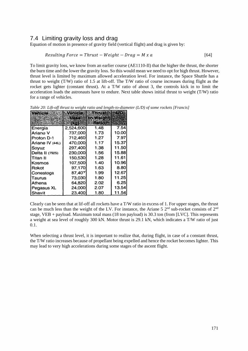
171
7.4 Limiting gravity loss and drag Equation of motion in presence of gravity field (vertical flight) and drag is given by:
𝑅𝑒𝑠𝑢𝑙𝑡𝑖𝑛𝑔 𝐹𝑜𝑟𝑐𝑒 = 𝑇ℎ𝑟𝑢𝑠𝑡 − 𝑊𝑒𝑖𝑔ℎ𝑡 − 𝐷𝑟𝑎𝑔 = 𝑀 𝑥 𝑎 [64]
To limit gravity loss, we know from an earlier course (AE1110-II) that the higher the thrust, the shorter
the burn time and the lower the gravity loss. So this would mean we need to opt for high thrust. However,
thrust level is limited by maximum allowed acceleration level. For instance, the Space Shuttle has a
thrust to weight (T/W) ratio of 1.5 at lift-off. The T/W ratio of course increases during flight as the
rocket gets lighter (constant thrust). At a T/W ratio of about 3, the controls kick in to limit the
acceleration loads the astronauts have to endure. Next table shows initial thrust to weight (T/W) ratio
for a range of vehicles.
Table 20: Lift-off thrust to weight ratio and length-to-diameter (L/D) of some rockets [Francis]
Clearly can be seen that at lif-off all rockets have a T/W ratio in excess of 1. For upper stages, the thrust
can be much less than the weight of the LV. For instance, the Ariane 5 2nd sub-rocket consists of 2nd
stage, VEB + payload. Maximum total mass (18 ton payload) is 30.3 ton (from [LVC]. This represents
a weight at sea level of roughly 300 kN. Motor thrust is 29.1 kN, which indicates a T/W ratio of just
0.1.
When selecting a thrust level, it is important to realize that, during flight, in case of a constant thrust,
the T/W ratio increases because of propellant being expelled and hence the rocket becomes lighter. This
may lead to very high accelerations during some stages of the ascent flight.
172
To limit drag loss, we need to limit the drag experienced by the LV. This is done by designing slender
vehicles with a high length-to-diameter ratio as in that case a low value of the drag coefficient can be
attained; see later in this course for more detailed info. From Table 20, we learn that typical L/D values
are in range 6 to 16. See later in this course for more on vehicle aerodynamics.
Example: Acceleration level
Consider a rocket of total mass 10 tons of which 9 tons are propellant. Maximum acceleration
allowed during flight is 6g. In addition, thrust of the rocket is constant.
Option 1: Thrust is identical to thrust at end of flight (maximum acceleration occurs at end of
flight). This gives a thrust level at end of flight of 1000 kg x 6 x 9.81 m/s2 = 58,860 N. Comparison
with the weight of the rocket at lift-off shows that the thrust is too low to ensure lift-off of the
rocket (rocket weight initially is 98100 N)
Option 2: Thrust is constant and is set equal to realize 1.2g acceleration at lift-off. This gives a
thrust of 117,720 N. However, at end of flight this gives an acceleration of 12g.
Note that in the above, we have neglected the effect of weight on the acceleration. This is
important when considering flight where there is a gravity component in the direction of flight,
like in vertical flight for launch from Earth surface into space. For space applications, most of
the time we aim to have the thrust force in a direction perpendicular to gravity and hence it has
no effect.
173
8. Velocity increment needed to launch into orbit A quick rough order of magnitude (ROM) estimate of the velocity increment needed to be in a
circular orbit at a specific altitude around some planet can be obtained by dividing the ΔV vector into
two components. One component is radial (normal) to the target orbit, the other is tangent to the target
orbit at the insertion point.
As the two vector components are perpendicular to each other, the sum of the two vectors is found
using Pythagoras rule. We write:
∆𝑣 = √(𝑣𝑡𝑎𝑛)2 + (𝑣𝑟𝑎𝑑)2
Here:
∆𝑣: is the required velocity increment
𝑣𝑡𝑎𝑛: is the velocity in the direction tangent to the target orbit.
𝑣𝑟𝑎𝑑: is the velocity in radial (vertical) direction of rocket at start of flight needed to attain the
required altitude. It is assumed that this velocity is the result of an impulsive burn of a very
short duration. Following the burn the mass of the vehicle is considered to remain constant
and kinetic energy is transferred to potential energy.
It is important to first lay out the assumptions that will be made. We will assume the following:
• The ∆𝑣 is provided by the launcher in one single burn.
• The burn is an impulsive shot.
• The mass of the launcher is taken right after the impulsive shot and constant during the entire
flight.
• The launcher is launched from the Earth surface from a launch site positioned along the
Equator.
• The target orbit is a circular orbit above the Earth.
• All the energy is transferred without losses due to drag, gravity, etc.
First, two elements contribute to the tangential velocity component. The first element is the orbital
velocity in the target circular orbit, which is the velocity at the end of the burn. The second element is
the initial velocity of the launcher, which is given by the rotation of the Earth.
The circular velocity at an altitude h can be determined with the Vis-Viva equation:
−𝜇
2𝑎 =
𝑣2
2 −
𝜇
𝑟
Therefore in the case of a circular orbit (where r = a ), the orbital velocity is :
𝑣𝑐𝑖𝑟𝑐 = √𝜇
𝑎
The initial velocity is given by the rotational velocity of the Earth at its surface. Depending on the
direction in which we launch, the velocity will not be the same. The magnitude of the rotational
velocity is computed with the Earth angular velocity (1 revolution in 24 hours) at a distance of the
Earth average radius Re = 6378 km . The magnitude of Vrot is :
174
𝑣𝑟𝑜𝑡 = 𝑅𝐸 2𝜋
𝑇𝑑𝑎𝑦 = 6378
2𝜋
24 × 60 × 60 = 0.465 𝑘𝑚/𝑠
If we launch towards the East, we are launching with the rotational movement and Vrot = 0.465 km/s.
When launching towards the West, we are launching against the rotational movement and
Vrot = - 0.465 km/s. When launching towards the North or the South, it can be assumed that
Vrot = 0 km/s.
The tangent velocity component can be computed by the difference between the end and beginning
velocities.
𝑣𝑡𝑎𝑛 = 𝑣𝑐𝑖𝑟𝑐 − 𝑣𝑟𝑜𝑡
Then, to determine the required radial velocity component of the rocket to be provided, consider the
rocket to be a ball. If you throw it with a certain initial velocity vertically upward, how high will it
get? Now consider what the initial speed must be in case you need to reach the orbital altitude h.
You have to consider that the radial velocity is kinetic energy (at start of flight) which is converted
into potential energy. Now since we are considering an impulsive shot, the rocket mass remains
constant during flight. Working out the equation gives (assuming gravity is constant and equal to
gravity at altitude):
𝑣𝑟𝑎𝑑 = √2𝑔ℎ
This uses the local gravity acceleration, which is a good approximation for lower altitudes (below
1000km). But as the launcher could go to higher altitudes, it is more precise to use an average gravity
acceleration between the surface and the target altitude.
The local gravitational acceleration can be calculated with:
𝑔𝑙𝑜𝑐𝑎𝑙 = 𝜇
(𝑅𝐸 + ℎ)²
Therefore the average acceleration is: 𝑔𝑎𝑣𝑔 = 𝑔0+ 𝑔𝑙𝑜𝑐𝑎𝑙
2
The radial velocity is: 𝑣𝑟𝑎𝑑 = √2𝑔𝑎𝑣𝑔ℎ
To conclude, the required velocity increment for a launch from a planet’s surface to a circular orbit
about that planet can be determined provided we know the gravitational acceleration at planet surface
level, the gravity parameter μ of the planet, the radius of the planet and the orbital altitude about the
planet.
Let’s show an example.
For a launch from Earth surface to a circular orbit at 300 km altitude using go = 9.81m/s2,
μ = 3.985 x10¹⁴ m3/s2 and REarth = 6378 km, we find:
𝑣𝑐𝑖𝑟𝑐 = √𝜇
𝑅𝐸 + ℎ= √
3.985 × 10¹⁴
6378000 + 300000= 7725 𝑚/𝑠
𝑔𝑎𝑣𝑔 =1
2 (𝑔0 +
𝜇
(𝑅𝐸+ℎ)²) = 9.373 𝑚/𝑠2

175
𝑣𝑟𝑎𝑑 = √2𝑔𝑎𝑣𝑔ℎ = √2 × 9.373 × 300000 = 2371 𝑚/𝑠
Finally, launching towards the East and taking 𝑣𝑟𝑜𝑡 = 465 m/s:
∆𝑣 = √(𝑣𝑐𝑖𝑟𝑐 − 𝑣𝑟𝑜𝑡)2 + (𝑣𝑟𝑎𝑑)2 = √(7725 − 465)2 + (2371)2 = 7637 𝑚/𝑠
If we were launching towards the North/South, taking 𝑣𝑟𝑜𝑡 = 0 m/s:
∆𝑣 = √(𝑣𝑐𝑖𝑟𝑐 − 𝑣𝑟𝑜𝑡)2 + (𝑣𝑟𝑎𝑑)2 = √(7725)2 + (2371)2 = 8.081 𝑚/𝑠
If we were launching towards the West, taking 𝑣𝑟𝑜𝑡 = - 465 m/s:
∆𝑣 = √(𝑣𝑐𝑖𝑟𝑐 − 𝑣𝑟𝑜𝑡)2 + (𝑣𝑟𝑎𝑑)2 = √(7725 + 465)2 + (2371)2 = 8.526 𝑚/𝑠

176
9. Parametric estimation
Parametric estimating refers to an estimation technique which is based on the premise that changes in
some output (dependent) parameter can be related to the value of an independent variable. For instance,
vehicle mass and size depend largely on payload mass and size or vehicle size depends on vehicle mass
or spacecraft cost can be related to spacecraft dry mass, etc. In general, we are looking for relations of
the form:
y = f(x)
Here y is the dependent variable and x is the independent variable. Above relation may be of different
forms, including linear, power, logarithmic, exponential, etc.
Parametric estimation relies on the use of relatively simple statistical analysis methods, like averaging
and regression analysis; to compress large amounts of data into more easily assimilated summaries,
which still provide the user with a sense of the content without overwhelming him/her. The most widely
used summary statistics are:
o Statistical analysis that provides a simple average (arithmeticetic or equally weighted mean),
and a sample standard deviation (SSD). The latter being a measure for the spread in the data.
o Regression analysis (a means of statistical analysis) that provides for a Most Likely Estimate
(MLE), i.e. “best curve fit of data”, and standard (percent) error of estimate (SEE) sometimes
also referred to as relative standard error (RSE).
Averaging generally is limited to the generation of linear relationships, whereas regression analysis also
allows for other types of relations to be developed.
A valuable aspect of parametric estimating is the higher levels of accuracy that can be built into it
depending on how sophisticated the original data that was built into the estimate turns out to have been.
A good understanding and an ability to determine mean and variance or standard deviation of a data
series is considered essential for this course. Some summary information on these terms is found in
appendix D. A further advantage of parametric estimation is that the estimation relationships can be
nicely combined with (more fundamental) relationships from physics (e.g. orbital mechanics), RAMS
engineering, etc.
Both similarity based and parametric estimation use data of more or less similar designs as a starting
point for the estimations. Important is to realize that the amount of data to be collected as well as the
analysis effort to be spent generally is highest in case of parametric estimation. Still, the latter method
has preference, because of its greater accuracy and because less expertise is needed for generating
estimations (more student friendly). Moreover, the latter method can also be applied in case no historic
missions can be found for estimation by similarity.
In this section, attention is focussed on developing/generation of estimations and/or estimation
relationships using historical data. The use of simple relationships from physics etc. will be illustrated
in later sections. Below, we will introduce first estimation using averaging and second using regression
analysis, i.e. “best curve fit of data”.
Estimation based on using arithmetic mean and standard deviation
In this section, we will introduce the use of averaging to develop a linear relation between an
independent and a dependent variable. We will do this by way of examples.
The first example is on the development of a relationship between S/C dry mass (the dependent variable)
and payload mass (the independent variable). We will do this based on the presumption that payload
mass is a fixed percentage or ratio of vehicle dry mass.
= dry payloadM A M [1]

177
Please consider what other parameters may affect the dry mass of the S/C. Consider e.g. the propellant
mass carried and more specifically the delta-v capability of the craft.
To allow for estimation of the value of the parameter A (which is here defined as the payload mass-to-
dry mass ratio), we have collected historical data on payload mass and dry mass as can be found in
literature. These data are given in Table 1. The table also provides the calculated value of the payload
mass-to-dry mass ratio.
Table 1: Sample mass data
Spacecraft Payload
mass
Vehicle dry
mass
Mass
fraction
(kg) (kg) (-)
A 220 750 0.29
B 36 250 0.14
C 43 420 0.10
D 12 112 0.11
E 25 140 0.18
Using the data from the foregoing table, we find an average payload mass to spacecraft dry mass ratio
of:
(0.29 0.14 0.10 0.11 0.18)0.16
5
+ + + += =x
An average mass fraction means that the constant “A” in the relation = 1/0.16 = 6.25 kg of dry mass for
every 1 kg of payload mass. Hence, it follows that vehicle dry mass is 6.25 times payload mass. So for
a payload mass of 100 kg, we find a vehicle dry mass of 625 kg.
Comparing the average mass fraction of 0.16 with the mass fractions of the individual vehicles some
spread is noticed. As a measure for the spread we determine the SSD using:
( )2
i
1SSD = x x
n 1 −
− [2]
Filling in numbers gives:
( ) ( ) ( ) ( ) ( )2 2 2 2 21
SSD = 0.13 0.02 0.06 0.05 0.02 0.085 1
+ − + − + − + = −
It follows an SSD of ~0.08 (more exactly 0.077) or roughly 50% of the average value of the fraction.
When assuming a normal distribution1 of the data, see appendix E, this means that roughly 65% of all
predicted values are within 50% (once the sample standard deviation) of the predicted value. So for a
100 kg payload mass, we find a dry vehicle mass of 625 kg. With a 65% probability, the dry mass is in
the mass range 417 kg – 1250 kg. That is how accurate it is!
Now when collecting data the issue might arise on how many data points are needed. For instance, when
taking only the first data point of Table 1, we have a fraction of 0.29, when adding the second, the mean
value is 0.22 and so on. The issue is when to stop or what is a statistically meaningful number? This
question is dealt with in numerous text books on statistics. For now, it is advised to use at least 10 data
points.
A second example of using averaging is based on the presumption that insurance cost is related to the
insured value. Some typical data for the period 1980 to 2002 is shown in Figure 1. From the data, we
1 Other distributions may exist. For the purpose of this work this will be left out of consideration.

178
find an average insurance rate over the period up to 2002 of 16.5% of the insured value. The figure also
clearly shows that from year to year variations do occur. To take into account these variations, the SSD
has been determined. A very approximate (exact figures are hard to obtain from the figure)
determination gives an SSD of 5.5%, meaning that 95% of all interest rates are in the range 5.5 – 27.5%
(average value ± 2 times SSD).
Figure 1: Insurance rates [Futron, 2002]
Above two examples are just two examples. Many more relations can be considered and some may
even be better than the ones presented here. This though is left for the reader to explore for her/himself.
Estimation using regression analysis and relative standard error (RSE)
Next to simple averaging, we can use regression analysis to determine relationships. Regression
analysis is a statistical process for estimating relationships among variables. It allows for a multitude of
relationships to be considered other than just the simple averaging discussed in the previous section.
For instance, we may also consider non-linear relations, but also relationships where the dependent
variable is a function of a multitude of independent variables. Details on linear regression will follow
in a later course. For now, we will limit ourselves to the use of for instance Microsoft Excel to determine
relatively simple regression relationships. When using Excel to generate regression relationships (trend
lines), the data must first be plotted in a graph. Generally the independent variable is along the x-
coordinate, whereas the dependent variable is taken along the y-coordinate. Once the data are plotted,
we can select the data in the figure and then add a trend line from a number of options. Options include
linear, power, exponential, logarithmic and polynomial. A typical example of a trend line plotted in a
data figure is given in Figure 2, which shows S/C gross (or total) mass (dry mass + propellant mass)
versus payload mass for interplanetary orbiter S/C. Below, we first discuss the regression line itself.
Following, we will discuss the data spread about this line.

179
Figure 2: Gross mass of some planetary spacecraft
The relationship found is referred to as estimating relationship and in this case it is a Mass Estimation
Relationship (MER) as the dependent variable in the relationship is mass. The value estimated for a
given value of the independent variable x (here the payload mass) is referred to as Most Likely Estimate
(MLE). Notice that other than for a linear relationship determined based on averaging; here the curve
not only has a slope, but also an intercept with the y-axis different from zero. More details on this
relationship can be found in appendix C.
When comparing the actual data with the regression line, it follows that there is a considerable spread
of data about this line. Reasons for the spread are that in reality spacecraft mass does depend on more
parameters that just payload mass. Consider for instance the effect of launch loads and size (not mass)
of payloads on spacecraft mass. Now accepting the spread as being real (no data errors), it is important
to have a measure for how well the regression curve fits the actual data. A figure of merit used in Excel
to determine the goodness of fit is the R2 value (R-squared value). The closer this value is to 1, the
better the fit; a value of 0 indicates there is essentially no fit. No further explanation is offered. Another
more readily understandable measure is the (relative) standard error of estimate (RSE), defined as:
𝑅𝑆𝐸 =2
ni
i 1 i
y11
n m f (x )=
−
− [3]
Here n is again the number of observed values, i.e. number of data points, m is number of parameters
estimated, yi is the real or actual value and f(xi) denotes the function value, i.e. the estimated value at
the point i. The value of “m” depends on the type of curve used. For a linear curve with an intercept at
y = 0 we have m = 1 and in case of an intercept different from zero, we have m = 2. To further illustrate
the meaning of m, consider determining a linear relationship between y (dependent variable) and x. The
linear relation (y = ax + b) has two unknown constants, i.e. the slope a, and the intercept b. this means
that we need to use two data points (minimum) to solve for the two unknowns. This leaves only (n-m)
data points for determining the RSE. Now consider that we have only two data points. This means that
both data points are needed to generate the straight line. By definition then the RSE is zero.
Notice that in the way that the RSE is defined here, it represents a relative error and is expressed as a
fraction of the estimated value. When multiplying this fraction with 100%, it can also be considered as
a percentage error. The reason for considering the relative error instead of the absolute error, as for the
SSD, is that the relative error can be considered more or less constant along the curve, whereas the
absolute error varies. This is illustrated in Figure 3 for the dry mass of interplanetary spacecraft in
relation to payload mass. The solid line in the figure represents the MER. The small diamonds are the
data points. The data spread about the MER is clearly visible. Now, when considering the magnitude of
the difference between the real and the predicted value, we find that this increases, with increasing
payload mass. However, when considering the relative error, this seems to remain within certain limits.
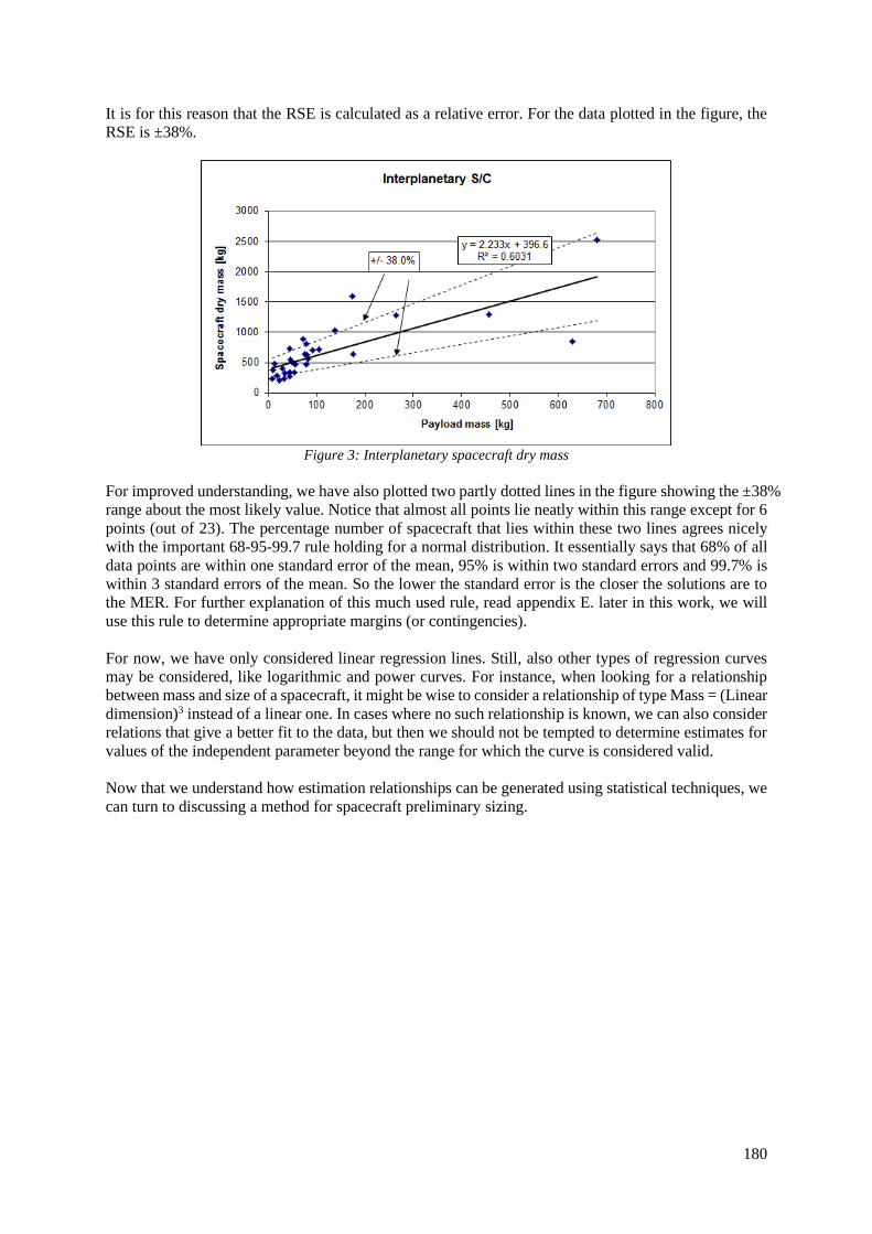
180
It is for this reason that the RSE is calculated as a relative error. For the data plotted in the figure, the
RSE is ±38%.
Figure 3: Interplanetary spacecraft dry mass
For improved understanding, we have also plotted two partly dotted lines in the figure showing the ±38%
range about the most likely value. Notice that almost all points lie neatly within this range except for 6
points (out of 23). The percentage number of spacecraft that lies within these two lines agrees nicely
with the important 68-95-99.7 rule holding for a normal distribution. It essentially says that 68% of all
data points are within one standard error of the mean, 95% is within two standard errors and 99.7% is
within 3 standard errors of the mean. So the lower the standard error is the closer the solutions are to
the MER. For further explanation of this much used rule, read appendix E. later in this work, we will
use this rule to determine appropriate margins (or contingencies).
For now, we have only considered linear regression lines. Still, also other types of regression curves
may be considered, like logarithmic and power curves. For instance, when looking for a relationship
between mass and size of a spacecraft, it might be wise to consider a relationship of type Mass = (Linear
dimension)3 instead of a linear one. In cases where no such relationship is known, we can also consider
relations that give a better fit to the data, but then we should not be tempted to determine estimates for
values of the independent parameter beyond the range for which the curve is considered valid.
Now that we understand how estimation relationships can be generated using statistical techniques, we
can turn to discussing a method for spacecraft preliminary sizing.
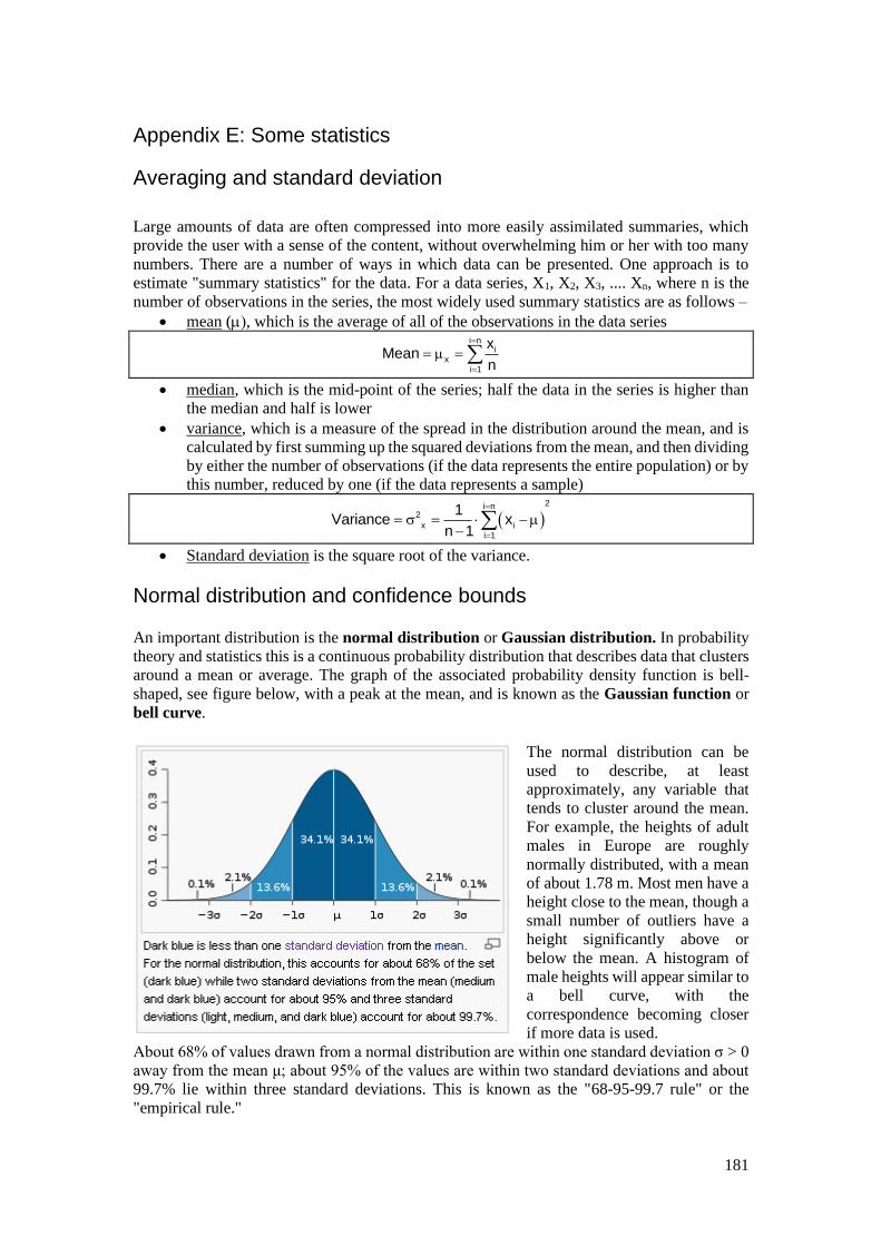
181
Appendix E: Some statistics
Averaging and standard deviation
Large amounts of data are often compressed into more easily assimilated summaries, which
provide the user with a sense of the content, without overwhelming him or her with too many
numbers. There are a number of ways in which data can be presented. One approach is to
estimate "summary statistics" for the data. For a data series, X1, X2, X3, .... Xn, where n is the
number of observations in the series, the most widely used summary statistics are as follows –
• mean (), which is the average of all of the observations in the data series i n
ix
i 1
xMean
n
=
=
= =
• median, which is the mid-point of the series; half the data in the series is higher than
the median and half is lower
• variance, which is a measure of the spread in the distribution around the mean, and is
calculated by first summing up the squared deviations from the mean, and then dividing
by either the number of observations (if the data represents the entire population) or by
this number, reduced by one (if the data represents a sample)
( )2i n
2
x ii 1
1Variance x
n 1
=
=
= = − −
• Standard deviation is the square root of the variance.
Normal distribution and confidence bounds
An important distribution is the normal distribution or Gaussian distribution. In probability
theory and statistics this is a continuous probability distribution that describes data that clusters
around a mean or average. The graph of the associated probability density function is bell-
shaped, see figure below, with a peak at the mean, and is known as the Gaussian function or
bell curve.
The normal distribution can be
used to describe, at least
approximately, any variable that
tends to cluster around the mean.
For example, the heights of adult
males in Europe are roughly
normally distributed, with a mean
of about 1.78 m. Most men have a
height close to the mean, though a
small number of outliers have a
height significantly above or
below the mean. A histogram of
male heights will appear similar to
a bell curve, with the
correspondence becoming closer
if more data is used.
About 68% of values drawn from a normal distribution are within one standard deviation σ > 0
away from the mean μ; about 95% of the values are within two standard deviations and about
99.7% lie within three standard deviations. This is known as the "68-95-99.7 rule" or the
"empirical rule."

182
What are Confidence Bounds?
One of the most confusing concepts to a novice engineer is estimating the precision of an
estimate or measurement. This is an important concept in the field of engineering, leading to
the use of confidence intervals (or bounds). In this section, we will try to briefly present the
concept in relatively simple terms but based on solid common sense.
The Black and White Marbles
To illustrate, consider the case where there are millions of perfectly mixed black and white
marbles in a rather large swimming pool and our job is to estimate the percentage of black
marbles. The only way to be absolutely certain about the exact percentage of marbles in the
pool is to accurately count every last marble and calculate the percentage. However, this is too
time-0 and resource-intensive to be a viable option, so we need to come up with a way of
estimating the percentage of black marbles in the pool. In order to do this, we would take a
relatively small sample of marbles from the pool and then count how many black marbles are
in the sample.
Taking a Small Sample of Marbles
First, pick out a small sample of marbles and count the black ones. Say you picked out ten
marbles and counted four black marbles. Based on this, your estimate would be that 40% of the
marbles are black.
If you put the ten marbles back in the pool and repeat this example again, you might get six
black marbles, changing your estimate to 60% black marbles. Which of the two is correct? Both
estimates are correct! As you repeat this experiment over and over again, you might find out
that this estimate is usually between X1% and X2%, and you can assign a percentage to the
number of times your estimate falls between these limits. For example, you notice that 90% of
the time this estimate is between X1% and X2%.
Taking a Larger Sample of Marbles
If you now repeat the experiment and pick out 1,000 marbles, you might get results for the
number of black marbles such as 545, 570, 530, etc., for
each trial. The range of the estimates in this case will be
much narrower than before. For example, you observe
that 90% of the time, the number of black marbles will
now be from Y1% to Y2%, where X1% < Y1% and
X2% > Y2%, thus giving you a more narrow estimate
interval. The same principle is true for confidence
intervals; the larger the sample size, the more narrow the
confidence intervals.
Confidence interval
If we perform ten identical tests on our units, and analyze the results, we will obtain slightly
different results each time. However, by employing confidence bounds, we obtain a range
within which these results are likely to fall. This range of plausible values is called a confidence
interval. Confidence bounds are generally described as being one-sided or two-sided.
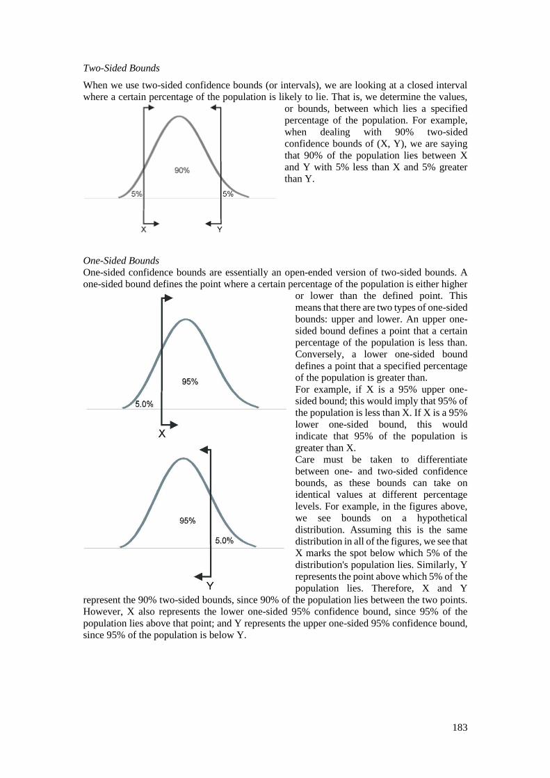
183
Two-Sided Bounds
When we use two-sided confidence bounds (or intervals), we are looking at a closed interval
where a certain percentage of the population is likely to lie. That is, we determine the values,
or bounds, between which lies a specified
percentage of the population. For example,
when dealing with 90% two-sided
confidence bounds of (X, Y), we are saying
that 90% of the population lies between X
and Y with 5% less than X and 5% greater
than Y.
One-Sided Bounds
One-sided confidence bounds are essentially an open-ended version of two-sided bounds. A
one-sided bound defines the point where a certain percentage of the population is either higher
or lower than the defined point. This
means that there are two types of one-sided
bounds: upper and lower. An upper one-
sided bound defines a point that a certain
percentage of the population is less than.
Conversely, a lower one-sided bound
defines a point that a specified percentage
of the population is greater than.
For example, if X is a 95% upper one-
sided bound; this would imply that 95% of
the population is less than X. If X is a 95%
lower one-sided bound, this would
indicate that 95% of the population is
greater than X.
Care must be taken to differentiate
between one- and two-sided confidence
bounds, as these bounds can take on
identical values at different percentage
levels. For example, in the figures above,
we see bounds on a hypothetical
distribution. Assuming this is the same
distribution in all of the figures, we see that
X marks the spot below which 5% of the
distribution's population lies. Similarly, Y
represents the point above which 5% of the
population lies. Therefore, X and Y
represent the 90% two-sided bounds, since 90% of the population lies between the two points.
However, X also represents the lower one-sided 95% confidence bound, since 95% of the
population lies above that point; and Y represents the upper one-sided 95% confidence bound,
since 95% of the population is below Y.

184
Most Likely Estimate (MLE) and Standard Error of estimate (SE)
A parametric relationship attempts to explain one variable, which is called the dependent
variable, using the other variable, called the independent variable. Parametric relationships
essentially can be of any form (linear, quadratic, power, log, etc.). For instance Excel allows
for determining such estimating relationships. It seeks the line that fits the data best. Goodness
of fit is expressed by R2 value. The closer this value is to 1, the better the fit.
Another way of expressing the goodness of fit is to determine the Standard Error of estimate
(SE):
Here ii
i
y
f(x ) = is referred to as multiplicative (or relative error) error, n is number of observed
values, m is the number of parameters being estimated, f(x) is estimate and y is true or actual
value of the parameter.
Dealing with uncertainty
In case of summing up various estimates like summing up the mass of the various subsystems
to arrive at a total system mass, the standard error (or sample standard deviation) of the sum is
given by the square root of the sum of the squares of the individual (absolute) errors, provided
that the individual estimates are independent (uncorrelated data) from each other:
2
i
i 1
SE SE=
=
In case of dependent or perfectly correlated variables, the SE is given by:
i
i 1
SE SE=
=
In case we are dealing with of SSD, identical rules apply.
Example: For a S/C you have estimated a payload cost of 40 M€ with a standard error (or
sample standard deviation) of 4 M€ and a bus cost of 30M€ 6 M€. Total cost of the S/C is
30 M€ + 40 M€ = 70 M€ with an uncertainty of:
1. maximum 10 M€ in case a rise in cost of the payload leads to an equal rise in bus cost;
2. maximum (42 + 62) 0.5 = 7.2 M€ in case a rise in cost of the payload has no effect on the
cost of the bus.
−
−=
2
i
i 1)x(f
y
mn
1SE

185
Appendix H: Earth Satellite Parameters
Table adapted from the
book Space Mission
Analysis and Design, by
Larson and Wertz,
Microcosm Press.
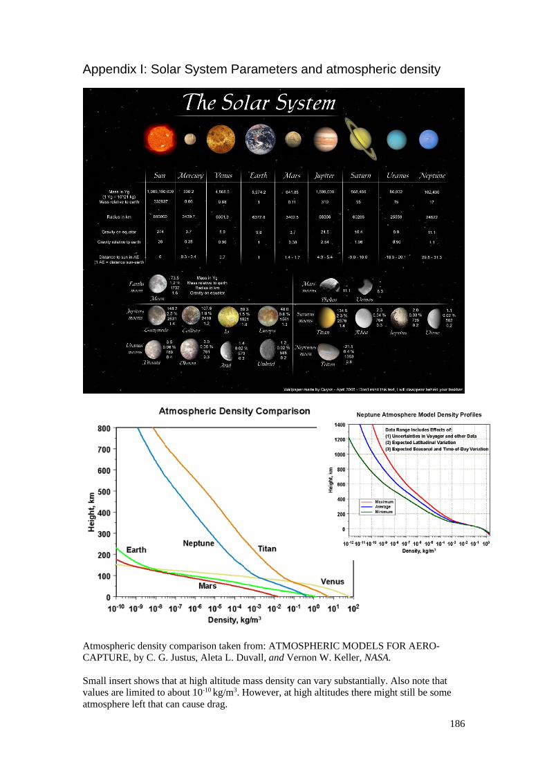
186
Appendix I: Solar System Parameters and atmospheric density
Atmospheric density comparison taken from: ATMOSPHERIC MODELS FOR AERO-
CAPTURE, by C. G. Justus, Aleta L. Duvall, and Vernon W. Keller, NASA.
Small insert shows that at high altitude mass density can vary substantially. Also note that
values are limited to about 10-10 kg/m3. However, at high altitudes there might still be some
atmosphere left that can cause drag.