Embed Size (px)
Citation preview

1
INTERNSHIP DOCUMENTATION
RTDS/RSCAD Type-3 Doubly-Fed Induction Wind Turbine Generator Model MANUAL
Leonel Noris (4627164)
TenneT TSO B. V. – TenneT TSO GmbH
TU Delft EEMCS
Contact Details

2
Internal TU Delft Supervisor
Dr. José Rueda Torres
Assistant Professor, IEPG
+31 01 5278 6239
TenneT Supervisor
Dr. Sven Rüberg
Asset Management
+49 176 26965371
TU Delft Student
Leonel Noris
Student of MSc Electrical Engineering
+31 06 2532 0452

3
Foreword
This internship is part of the curriculum of the MSc Electrical Engineering (Track Electrical Sustainable
Energy) at the Faculty of Electrical Engineering, Mathematics and Computer Science (EEMCS) at TU
Delft. The internship aimed to get the student insight into some duties a professional electrical
engineer may execute in a foreign company, as well as apply the gained skills on the bachelor’s and
master’s in the job position. The student also acquired experience of being part of a teamwork with
a different dynamic of Academia. The internship duration was four months and started from August
2nd, 2017 until November 30th, 2017.
This report describes the tasks performed by the student, the tools utilized to perform such tasks,
and the results. The report also contains information about the student’s experience regarding his
professional experience into TenneT.
The tasks done in this internship were in fact done for the German branch of the Dutch power utility
TenneT (TenneT TSO GmbH). For administrative reasons, the internship was officially reported to
TenneT TSO B. V. (The Netherlands).
The student would like to thank his supervisors Mr. Alfredo Campos for smartly and extensively
supporting the student progress of the stage, Mr. Sven Rüberg for giving him the opportunity of
having such professional experience and Mr. José Rueda for his advice and for push this student to
the limit.

4
Index
Project Development………………………………………………………………………………………………………………..
1. Mimic building of the different elements that conform the PSCAD Type-3 Model into
RSCAD…………………………………………………………………………………………………………………..
2. Debugging compilation errors on draft canvas in RSCAD…………………………………………….
3. Test of each sub model that composes the Type-3 Model drafted in RSCAD…………………
4. Integration of all the elements of the model into one big model………………………………….
5. Settings for the complete Type-3 WTG Model……………………………………………………………
6. Project Outcome: Test and validation of the Type-3 WTG Model…………………………………
Results-Initial conditions of 17 m/s and 56 active units-No faults…………………………..
Results-Initial conditions of 17 m/s and 56 active units-Short-Circuit Fault in Phase
A-to-Ground……………………………………………………………………………………………………..
Instructions for tuning the model parameters………………………………………………………………………………
Instructions for running the simulation……………………………………………………………………………………….
Glossary………………………………………………………………………………………………………………………………….
References………………………………………………………………………………………………………………………………
5
5 35
35 37 37 40 48
51
60
63
66
52

5
Project Development
• Description of the activities achieved during the internship.
The official name of the DFIG wind turbine model created in PSCAD is DFIG_PE_Tennet_V14. The
activities started with a one-week tutorial for learning how to use the RSCAD software tool. Then the
student went over the description manuals of the mentioned PSCAD wind turbine model [5] to be
translated from software to software to understand its structure, its functions and systems. Once the
wind turbine model developed in the PSCAD tool was delivered, the next stage was to build in image
and likeness the Type-3 model by parts. Figure 1 and Figure 2 show the layout of the DFIG model
created in PSCAD with its grid-side and rotor-side converter controls. After finishing the construction
of each partial draft, the student performed tests on such model to verify that each small component
of the whole draft behaved the same way as the original PSCAD model, presenting similar
performances in graphical plots, resulting in similar numerical values of the signals or wirelabels
related to each plot and draft. Once each component of the Type-3 WTG model was constructed and
tested separately, the next stage was to build the whole draft model, by linking all the puzzle pieces,
and furthermore doing the last tests for the whole system. The goals achieved up to November 30th,
2017 (date of the internship termination) were the following.
1. Mimic building of the different elements that conform the PSCAD Type-3 Model into
RSCAD
Figure 1. PSCAD Type-3 Wind Turbine Model.
Figure 2. PSCAD Type-3 Wind Turbine GSC/RSC controls.
6
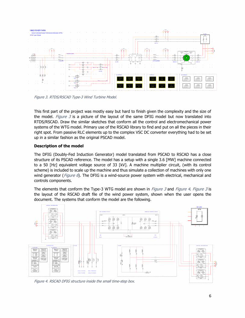
This first part of the project was mostly easy but hard to finish given the complexity and the size of
the model. Figure 3 is a picture of the layout of the same DFIG model but now translated into
RTDS/RSCAD. Draw the similar sketches that conform all the control and electromechanical power
systems of the WTG model. Primary use of the RSCAD library to find and put on all the pieces in their
right spot. From passive RLC elements up to the complex VSC DC converter everything had to be set
up in a similar fashion as the original PSCAD model.
Description of the model
The DFIG (Doubly-Fed Induction Generator) model translated from PSCAD to RSCAD has a close
structure of its PSCAD reference. The model has a setup with a single 3.6 [MW] machine connected
to a 50 [Hz] equivalent voltage source of 33 [kV]. A machine multiplier circuit, (with its control
scheme) is included to scale up the machine and thus simulate a collection of machines with only one
wind generator (Figure 6). The DFIG is a wind-source power system with electrical, mechanical and
controls components.
The elements that conform the Type-3 WTG model are shown in Figure 3 and Figure 4. Figure 3 is
the layout of the RSCAD draft file of the wind power system, shown when the user opens the
document. The systems that conform the model are the following.
Figure 3. RTDS/RSCAD Type-3 Wind Turbine Model.
Figure 4. RSCAD DFIG structure inside the small time-step box.
7
Mechanical system
The mechanical system takes care of simulate the collection of wind, which be translated into the
mechanical energy, which derivates in the torque of the blades and rotor of the aerogenerator, thus
converting the maximum power available from the wind to torque. The interface component (from
mechanical to electrical) in this system is the induction generator (Figure 9), which converts the
mechanical energy into electrical energy. In the parameters of this component can be found signal
input TL, which is the mechanical input signal calculated in the circuit shown in Figure 32 and signal
output TE, which is the respective electric torque.
Electrical system
The electrical system converts the input mechanical power into electrical and delivers such power
into the electrical power grid. The electrical system is the largest and most complex part of this
model. This model was based on the PSCAD wind farm EMT model named DFIG_PE_Tennet_V14,
which is a model that includes the power electronic converters, as can be inferred by the PE acronym.
All power electronics components in the model are placed inside the small time-step hierarchical box.
This reference model, with power electronic switches, provides a complete simulation of the system
for dynamic and harmonic analysis while keeping the balance of power. The disadvantage of using
the average model is that its power electronic converters make it complex and slower for running a
simulation, and the harmonic oscillations can be noticed in many of the plots that deforms them,
especially when simulating a larger number of aerogenerators with the machine scaling.
The DFIG is connected to the AC system through a three-winding transformer (Figure 8). Further,
can be seen a back-to-back power electronics bridge, with the grid-side converter (GSC) and the
rotor-side converter (RSC). The GSC objective is to maintain the DC bus voltage, while the RSC
oversees injecting the appropriate currents to the rotor circuit of the induction machine, such that
the desired active and reactive power P, Q are obtained at the stator terminals of the machine. Both
converters are connected back-to-back through a DC bus with a capacitor, whose voltage is defined
through the signal Edc. Both converters are operated as Voltage Source Converters (VSC). The back-
to-back VSC converter also includes a chopper in its DC interface, whose signal name is RCHOPPER.
The chopper is used to protect the DC bus from overvoltages. Outside the converter, on the rotor-
side, can be found a crowbar circuit, with a six-diode structure and a GTO thyristor. The crowbar is
used to protect the rotor side converter against current surges coming from the machine rotor–side
circuit. Next to the converter, can be found an AC filter, which is used to remove some of the voltage
harmonics introduced by the two-level converter.
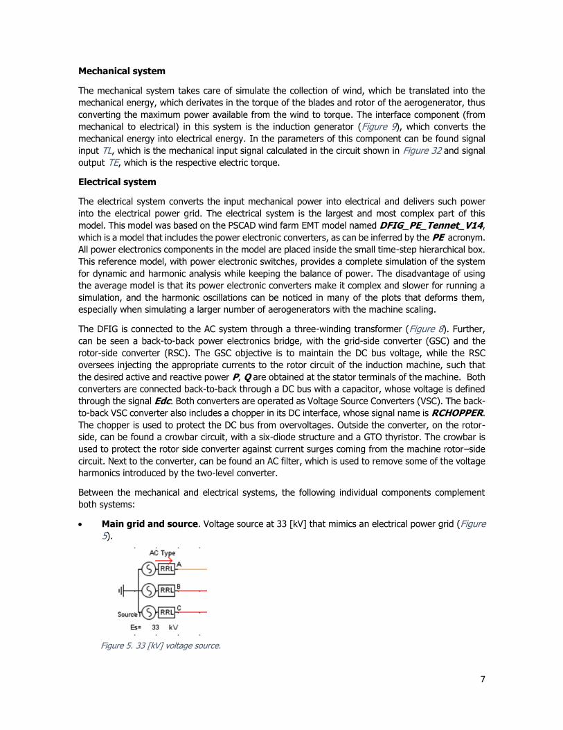
Between the mechanical and electrical systems, the following individual components complement
both systems:
• Main grid and source. Voltage source at 33 [kV] that mimics an electrical power grid (Figure
5).
Figure 5. 33 [kV] voltage source.

8
• Multimeters. Meters that sense and read instant voltages, instant currents, RMS voltages,
active power P and reactive power Q. They are located in several parts of the model structure
(Figure 6).
• Controls processors. These parameters are used to assign all the control systems and the
electric circuits components to several physical processor units in the RTDS hardware (Figure
7). Important to order each component of the model draft in a convenient way to optimize the
power capabilities of calculation and plotting of the results given in the runtime simulation
window, as shown in Figure 69.
• Three-phase transformer. Its primary winding is connected to the electric power grid, with
a voltage of 33 [kV]. Its secondary winding is connected to the left-side of the VSC back-to-
back converter with 0.69 [kV]. Its tertiary winding is connected to the induction generator at
0.9 [kV] (Figure 8). The parameters to set were the same as the ones found in the reference
PSCAD model.
Figure 6. Multimeters.
Figure 7. Controls processors.
Figure 8. Three-phase transformer.
9
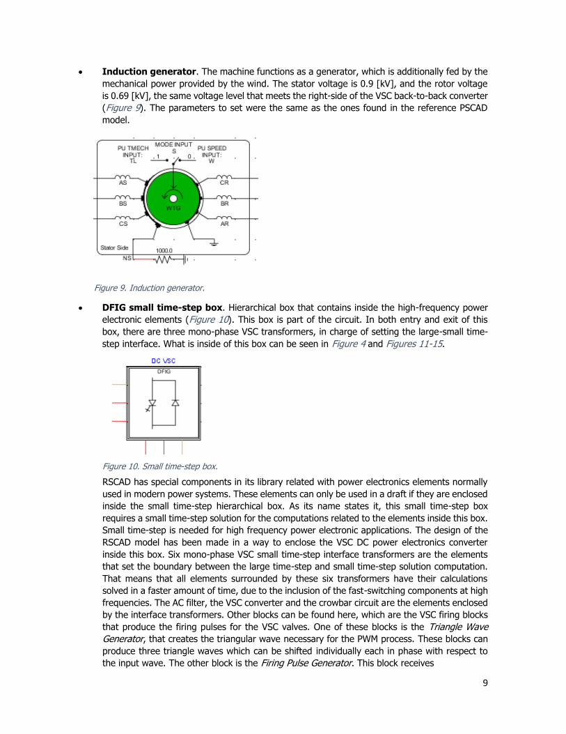
• Induction generator. The machine functions as a generator, which is additionally fed by the
mechanical power provided by the wind. The stator voltage is 0.9 [kV], and the rotor voltage
is 0.69 [kV], the same voltage level that meets the right-side of the VSC back-to-back converter
(Figure 9). The parameters to set were the same as the ones found in the reference PSCAD
model.
• DFIG small time-step box. Hierarchical box that contains inside the high-frequency power
electronic elements (Figure 10). This box is part of the circuit. In both entry and exit of this
box, there are three mono-phase VSC transformers, in charge of setting the large-small time-
step interface. What is inside of this box can be seen in Figure 4 and Figures 11-15.
RSCAD has special components in its library related with power electronics elements normally
used in modern power systems. These elements can only be used in a draft if they are enclosed
inside the small time-step hierarchical box. As its name states it, this small time-step box
requires a small time-step solution for the computations related to the elements inside this box.
Small time-step is needed for high frequency power electronic applications. The design of the
RSCAD model has been made in a way to enclose the VSC DC power electronics converter
inside this box. Six mono-phase VSC small time-step interface transformers are the elements
that set the boundary between the large time-step and small time-step solution computation.
That means that all elements surrounded by these six transformers have their calculations
solved in a faster amount of time, due to the inclusion of the fast-switching components at high
frequencies. The AC filter, the VSC converter and the crowbar circuit are the elements enclosed
by the interface transformers. Other blocks can be found here, which are the VSC firing blocks
that produce the firing pulses for the VSC valves. One of these blocks is the Triangle Wave
Generator, that creates the triangular wave necessary for the PWM process. These blocks can
produce three triangle waves which can be shifted individually each in phase with respect to
the input wave. The other block is the Firing Pulse Generator. This block receives
Figure 10. Small time-step box.
Figure 9. Induction generator.

10
Figure 11. Large-small time-step interface of the GSC.
Figure 12. Crowbar circuit.
Figure 13. VSC DC converter.
Figure 15. AC filter. Figure 14. Triangle-wave and firing-pulse generators for both GSC and RSC.

11
three different modulation waves, plus the signal of the triangular wave produced by the
Triangle Wave Generator. The RSCAD model has a pair of these two VSC PWM control boxes,
each for each side of the converter, since each extreme has a different carrier frequency,
expressed as multiple of the fundamental frequency. For the GSC the carrier frequency equals
60 and for the RSC equals 37.
Control components
The control components are all the command schemes that control the electro-mechanical system
that make possible dynamic and harmonic stability and power managing, for any kind of input
parameters on steady state, and under the simulation of a fault. The control system of the model
also is the one that starts the initialization of the simulation, the process of linking the wind farm
with the electric power grid. The RSCAD model contains a group of logic schemes that set orders to
the different systems that compose the RSCAD WTG model, as shown in Figure 16. The model has
six main control schemes, which are:
• AC circuit breaker control. Circuit breaker that, once closed, starts the initialization
process for linking the wind farm with the electric power grid.
• Faults logic. Contains all the 11 different types of electric faults from phase-to-phase
to phase-to-ground faults (all combinations). The maximum duration of the faults can
be tune with a slider up to 0.3 [s].
• Machine scaling controls. Composed by a slider with a maximum limit of a hundred
aerogenerators, a rate-limiter that tunes the rate of change after increasing/decreasing
the number of active units. Minimum case is one active aerogenerator and maximum
case is a hundred active units.
• Wind park control. Controls the reactive power Q and active power P of the model
taking in account the scaling factor that simulates the wind park.
• Synchronizer block controls. Control system that defines the appropriate moment to
close the stator circuit breaker for completing the synchronizing process by setting
magnitude and phase voltage tolerances for minimum feasible conditions.
• DFIG controls. Supra-system that controls the doubly-fed induction generator.
AC circuit breaker and breaker control box
The first control scheme is the one in charge of closing the contacts of the AC circuit breaker.
It consists of a simple switch; whose signal name is Time Breaker Logic. Once switched ON,
starts the initialization process. It also gives names to the signals that de-block the Machine
Scaling control box (signal Dblk) and starts the sequence of the Synchronizer block box
Figure 16. Control schemes.
12
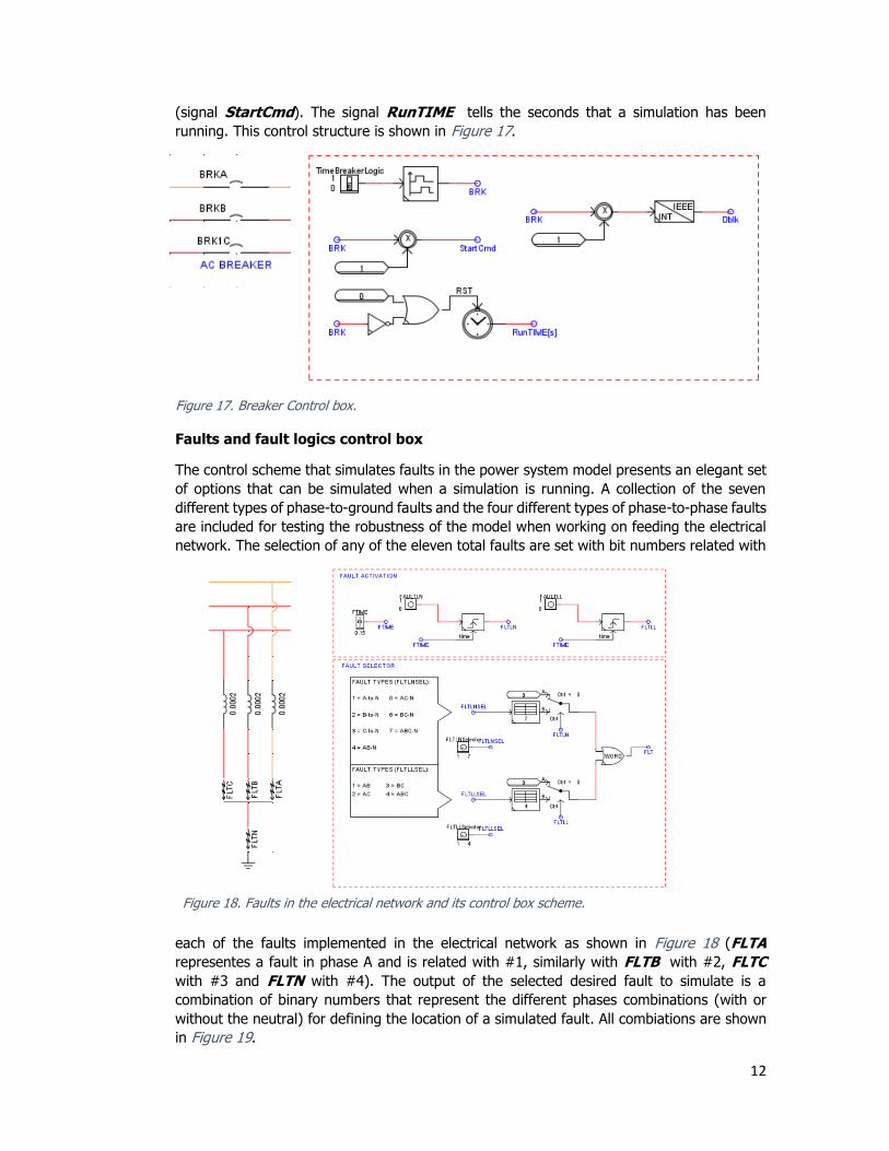
(signal StartCmd). The signal RunTIME tells the seconds that a simulation has been
running. This control structure is shown in Figure 17.
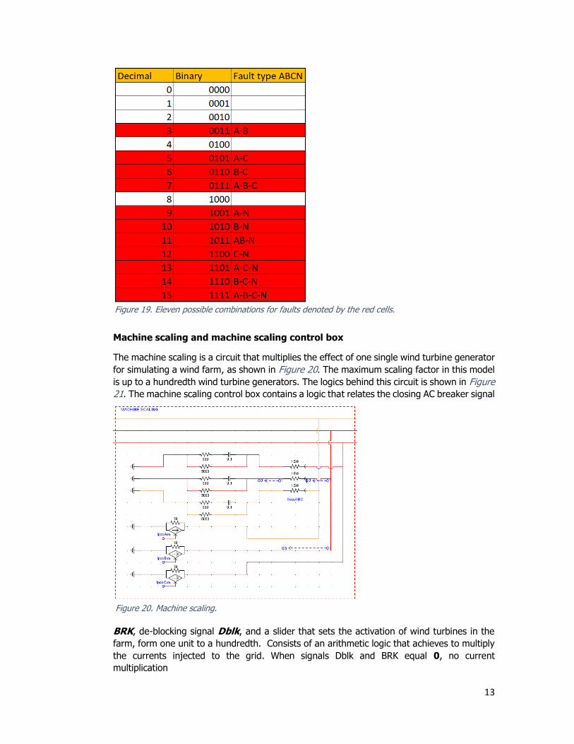
Faults and fault logics control box
The control scheme that simulates faults in the power system model presents an elegant set
of options that can be simulated when a simulation is running. A collection of the seven
different types of phase-to-ground faults and the four different types of phase-to-phase faults
are included for testing the robustness of the model when working on feeding the electrical
network. The selection of any of the eleven total faults are set with bit numbers related with
each of the faults implemented in the electrical network as shown in Figure 18 (FLTA
representes a fault in phase A and is related with #1, similarly with FLTB with #2, FLTC
with #3 and FLTN with #4). The output of the selected desired fault to simulate is a
combination of binary numbers that represent the different phases combinations (with or
without the neutral) for defining the location of a simulated fault. All combiations are shown
in Figure 19.
Figure 17. Breaker Control box.
Figure 18. Faults in the electrical network and its control box scheme.
13
Machine scaling and machine scaling control box
The machine scaling is a circuit that multiplies the effect of one single wind turbine generator
for simulating a wind farm, as shown in Figure 20. The maximum scaling factor in this model
is up to a hundredth wind turbine generators. The logics behind this circuit is shown in Figure
21. The machine scaling control box contains a logic that relates the closing AC breaker signal
BRK, de-blocking signal Dblk, and a slider that sets the activation of wind turbines in the
farm, form one unit to a hundredth. Consists of an arithmetic logic that achieves to multiply
the currents injected to the grid. When signals Dblk and BRK equal 0, no current
multiplication
Figure 20. Machine scaling.
Figure 19. Eleven possible combinations for faults denoted by the red cells.

14
can occur. But once those signals are activated, they equal 1. The larger the number of active
units, the larger the current flowing through each phase. The currents in each phase of the
circuit are represented by the Norton equivalents as seen in the circuit shown in Figure 20.
Wind park control box
Just like its PSCAD reference, the model includes a wind park controller to control multiple
wind turbines by sending a signal with a common reference setpoint. Figure 22 shows the
layout of that control scheme based on PSCAD’s translated into RTDS/RSCAD. What is inside
the hierarchical box WP controls and communications can be seen in Figure 23.
Figure 21. Machine scaling control box.
Figure 22. Wind park control box. The hierarchical box has the WP controls and communications.
15
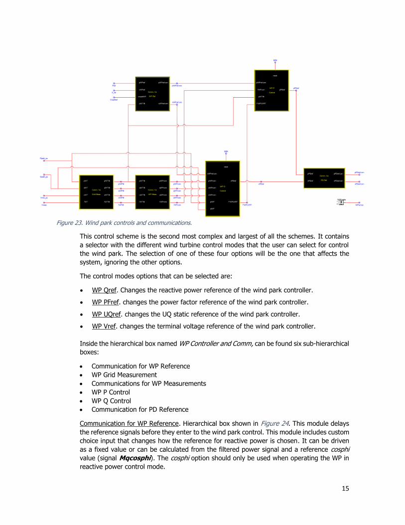
This control scheme is the second most complex and largest of all the schemes. It contains
a selector with the different wind turbine control modes that the user can select for control
the wind park. The selection of one of these four options will be the one that affects the
system, ignoring the other options.
The control modes options that can be selected are:
• WP Qref. Changes the reactive power reference of the wind park controller.
• WP PFref. changes the power factor reference of the wind park controller.
• WP UQref. changes the UQ static reference of the wind park controller.
• WP Vref. changes the terminal voltage reference of the wind park controller.
Inside the hierarchical box named WP Controller and Comm, can be found six sub-hierarchical
boxes:
• Communication for WP Reference
• WP Grid Measurement
• Communications for WP Measurements
• WP P Control
• WP Q Control
• Communication for PD Reference
Communication for WP Reference. Hierarchical box shown in Figure 24. This module delays
the reference signals before they enter to the wind park control. This module includes custom
choice input that changes how the reference for reactive power is chosen. It can be driven
as a fixed value or can be calculated from the filtered power signal and a reference cosphi
value (signal Mqcosphi). The cosphi option should only be used when operating the WP in
reactive power control mode.
Figure 23. Wind park controls and communications.

16
Figure 24. Communication for WP Reference.
Figure 25. WP Grid Measurement.
Figure 26. Communications for WP Measurements.
WP Grid Measurement. Hierarchical box shown in Figure 25. The purpose of this module is
to filter the power, voltage and frequency measurements at the grid.
Communications for WP Measurements. Hierarchical box shown in Figure 26. This module
delays the signals between the filtered grid measurements and the rest of the WP controller.
The delays can be obtained by using linear lead-lag function, which can be selected in the
properties of the module. The parameters of the delay can also be altered to meet any
demands.
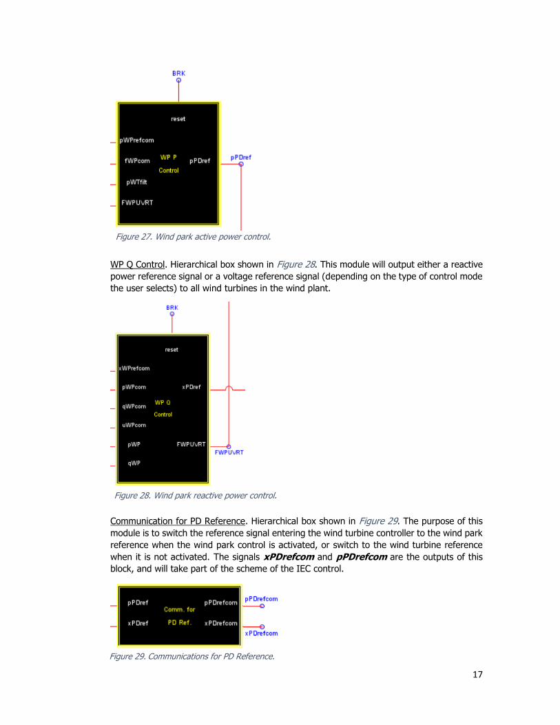
WP P Control. Hierarchical box shown in Figure 27. This module determines the reference
power signal (signal pPDref) to be sent to all wind turbines in the wind farm. The user can
also enable or disable a frequency dependent term that will either add to or subtract from
the power reference if the frequency is not held at 1.0 [pu] (Mfcontr).
17
Figure 14. WP P Control.
Figure 29. Communications for PD Reference.
Figure 27. Wind park active power control.
Figure 28. Wind park reactive power control.
WP Q Control. Hierarchical box shown in Figure 28. This module will output either a reactive
power reference signal or a voltage reference signal (depending on the type of control mode
the user selects) to all wind turbines in the wind plant.
Communication for PD Reference. Hierarchical box shown in Figure 29. The purpose of this
module is to switch the reference signal entering the wind turbine controller to the wind park
reference when the wind park control is activated, or switch to the wind turbine reference
when it is not activated. The signals xPDrefcom and pPDrefcom are the outputs of this
block, and will take part of the scheme of the IEC control.
18
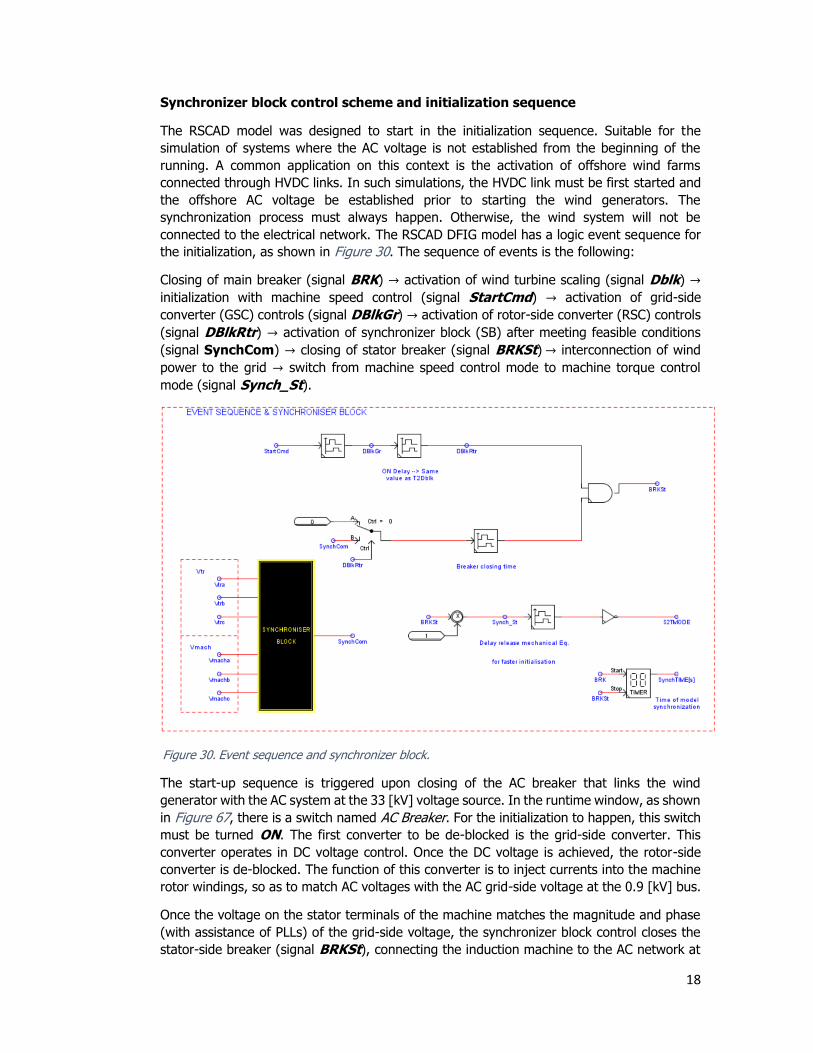
Figure 30. Event sequence and synchronizer block.
Synchronizer block control scheme and initialization sequence
The RSCAD model was designed to start in the initialization sequence. Suitable for the
simulation of systems where the AC voltage is not established from the beginning of the
running. A common application on this context is the activation of offshore wind farms
connected through HVDC links. In such simulations, the HVDC link must be first started and
the offshore AC voltage be established prior to starting the wind generators. The
synchronization process must always happen. Otherwise, the wind system will not be
connected to the electrical network. The RSCAD DFIG model has a logic event sequence for
the initialization, as shown in Figure 30. The sequence of events is the following:
Closing of main breaker (signal BRK) → activation of wind turbine scaling (signal Dblk) →
initialization with machine speed control (signal StartCmd) → activation of grid-side
converter (GSC) controls (signal DBlkGr) → activation of rotor-side converter (RSC) controls
(signal DBlkRtr) → activation of synchronizer block (SB) after meeting feasible conditions
(signal SynchCom) → closing of stator breaker (signal BRKSt) → interconnection of wind
power to the grid → switch from machine speed control mode to machine torque control
mode (signal Synch_St).
The start-up sequence is triggered upon closing of the AC breaker that links the wind
generator with the AC system at the 33 [kV] voltage source. In the runtime window, as shown
in Figure 67, there is a switch named AC Breaker. For the initialization to happen, this switch
must be turned ON. The first converter to be de-blocked is the grid-side converter. This
converter operates in DC voltage control. Once the DC voltage is achieved, the rotor-side
converter is de-blocked. The function of this converter is to inject currents into the machine
rotor windings, so as to match AC voltages with the AC grid-side voltage at the 0.9 [kV] bus.
Once the voltage on the stator terminals of the machine matches the magnitude and phase
(with assistance of PLLs) of the grid-side voltage, the synchronizer block control closes the
stator-side breaker (signal BRKSt), connecting the induction machine to the AC network at

19
0.9 [kV]. The synchronizer block checks minimum feasible conditions for voltages and phases
by means of a simplified algorithm that checks voltage ∆𝑉 and angle ∆𝛿 differences. The
synchronizer block assumes that the different frequencies are tuned properly because the
RSC controls are locked to the system frequency by means of the PLL related to it. Once that
the stator circuit breaker has closed its contacts, the machine is ready to start transferring
active power into the network. In this stage, the only control scheme not related with the
synchronization process if the Faults Logic control box.
The signal SynchTIME tells the time that the wind power system takes to realize the
synchronization sequence. The time that takes the synchronization sequence to realize in the
PSCAD model under any initial conditions is around one second. For the RSCAD model this
varies according to the initial parameters, but the synchronizing sequence should happen
before one minute. After several tests, the synchronization sequence in the RSCAD model
never could be as fast as the model built in PSCAD.
The voltages to be measured by the synchronizer block are the three-phase transformer
voltages Vtra, Vtrb and Vtrc, and the induction machine stator voltages Vmacha, Vmachb
and Vmachc, which are the signals that enter the synchronizer block as shown in Figure 31.
Figure 31. Inside the synchronizer block.
20
DFIG controls
Of all control schemes, the most extensive and complex one is the DFIG controls box, since
inside it, all the controllers for the mechanical and electrical systems of the wind power
system can be found. This hierarchical box has seven different control schemes, represented
by the following sub-components:
• Wind turbine mechanical power
• Induction machine control modes
• Grid-side converter controls
• Rotor-side converter controls
• Crowbar protection
• Chopper protection
• IEC controls
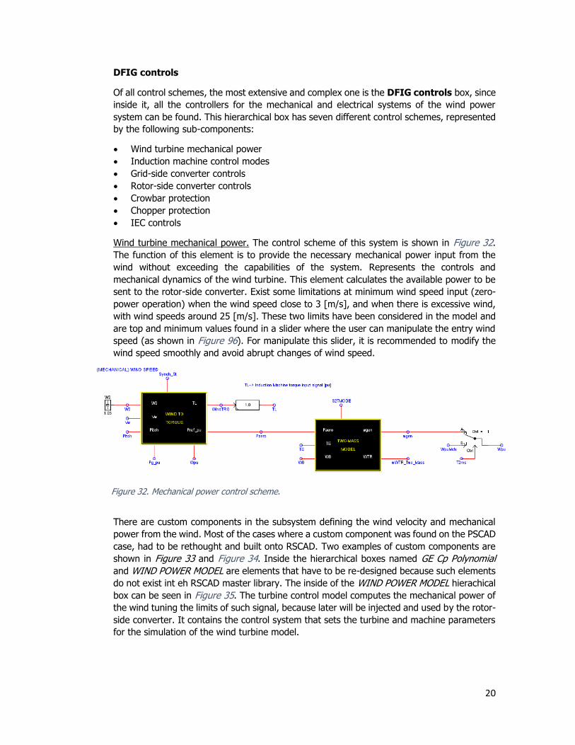
Wind turbine mechanical power. The control scheme of this system is shown in Figure 32.
The function of this element is to provide the necessary mechanical power input from the
wind without exceeding the capabilities of the system. Represents the controls and
mechanical dynamics of the wind turbine. This element calculates the available power to be
sent to the rotor-side converter. Exist some limitations at minimum wind speed input (zero-
power operation) when the wind speed close to 3 [m/s], and when there is excessive wind,
with wind speeds around 25 [m/s]. These two limits have been considered in the model and
are top and minimum values found in a slider where the user can manipulate the entry wind
speed (as shown in Figure 96). For manipulate this slider, it is recommended to modify the
wind speed smoothly and avoid abrupt changes of wind speed.
There are custom components in the subsystem defining the wind velocity and mechanical
power from the wind. Most of the cases where a custom component was found on the PSCAD
case, had to be rethought and built onto RSCAD. Two examples of custom components are
shown in Figure 33 and Figure 34. Inside the hierarchical boxes named GE Cp Polynomial
and WIND POWER MODEL are elements that have to be re-designed because such elements
do not exist int eh RSCAD master library. The inside of the WIND POWER MODEL hierachical
box can be seen in Figure 35. The turbine control model computes the mechanical power of
the wind tuning the limits of such signal, because later will be injected and used by the rotor-
side converter. It contains the control system that sets the turbine and machine parameters
for the simulation of the wind turbine model.
Figure 32. Mechanical power control scheme.

21
What is described in that box is the following formula:
𝑃 =𝜌
2× 𝐴𝑟 × 𝑉𝑊
3 × 𝐶𝑝(𝜆, 𝜃)
where
𝑃 - Mechanical power extracted from the wind turbine;
ρ - Air density in 𝑘𝑔
𝑚3;
𝐴𝑟 - Area swept by the rotor blades in m2;
𝑉𝑊 - Wind speed in 𝑚
𝑠𝑒𝑐;
𝜆 - Tip speed ratio
𝜃 - Pitch angle
𝐶𝑝 - Power coefficient, which is function of 𝜆 and 𝜃.𝐶𝑝 is a characteristic of the wind turbine that is
usually provided by the manufacturer as a set of curves relating 𝐶𝑝 to 𝜆 with 𝜃 parameters.
Figure 34. Examples of custom components. Cp polynomial and Wind Power Model in RSCAD model version.
Figure 33. Examples of custom components. Cp polynomial and Wind Power Model.
Figure 35. Wind power model.
22
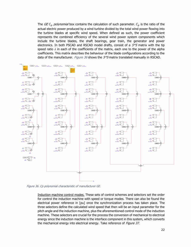
The GE 𝐶𝑝 polynomial box contains the calculation of such parameter. 𝐶𝑝 is the ratio of the
actual electric power produced by a wind turbine divided by the total wind power flowing into
the turbine blades at specific wind speed. When defined as such, the power coefficient
represents the combined efficiency of the several wind power system components which
include the turbine blades, the shaft bearings, gear train, the generator and power
electronics. In both PSCAD and RSCAD model drafts, consist of a 5*5 matrix with the tip
speed ratio 𝜆 in each of the coefficients of the matrix, each one to the power of the alpha
coefficients. This matrix describes the behaviour of the blade configurations according to the
data of the manufacturer. Figure 36 shows the 5*5 matrix translated manually in RSCAD.
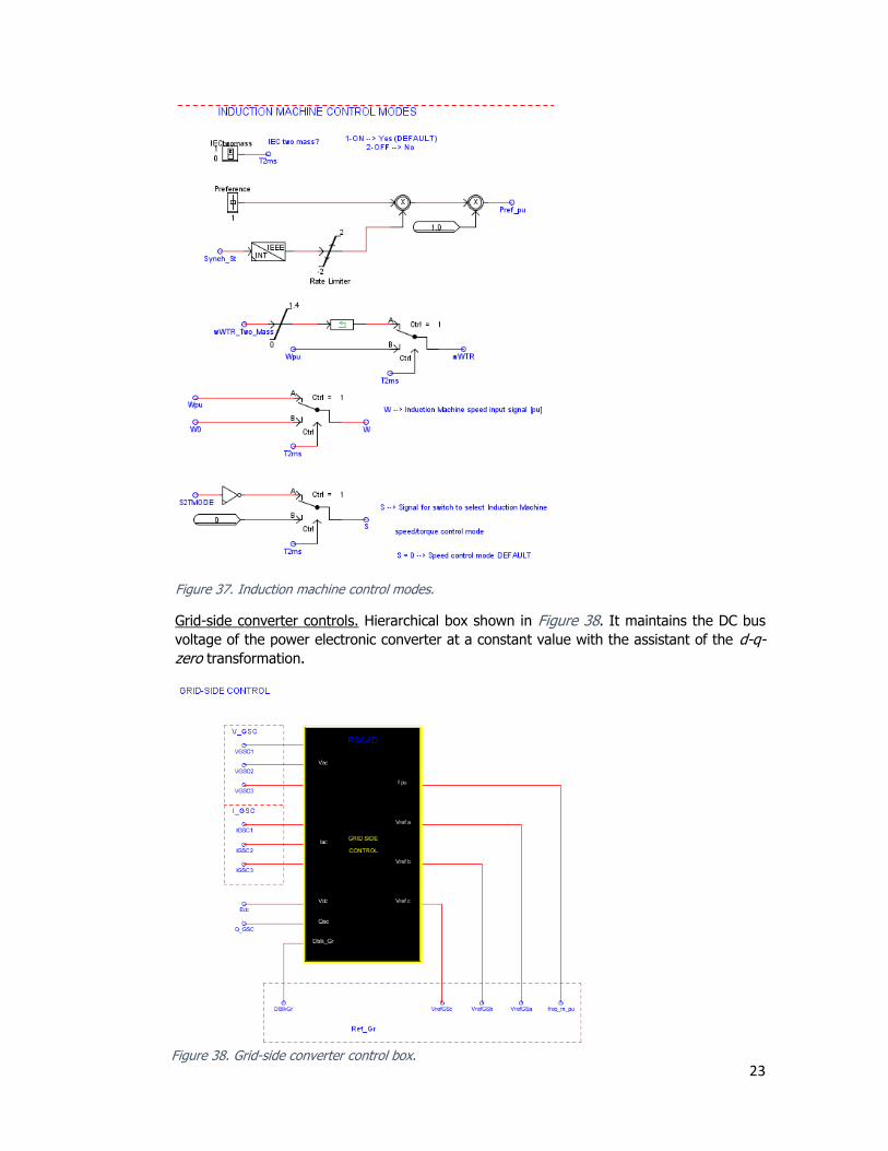
Induction machine control modes. These sets of control schemes and selectors set the order
for control the induction machine with speed or torque modes. There can also be found the
electrical power reference in [pu] once the synchronization process has taken place. The
three selectors define the calculated wind speed that then will be an input parameter for the
pitch angle and the induction machine, plus the aforementioned control mode of the induction
machine. These selectors are crucial for the process the conversion of mechanical to electrical
energy since the induction machine is the interface component in this system, which converts
the mechanical energy into electrical energy. Take reference of Figure 37.
Figure 36. Cp polynomial characteristic of manufacturer GE.
23
1.4.7
Grid-side converter controls. Hierarchical box shown in Figure 38. It maintains the DC bus
voltage of the power electronic converter at a constant value with the assistant of the d-q-
zero transformation.
Figure 37. Induction machine control modes.
Figure 38. Grid-side converter control box.
24
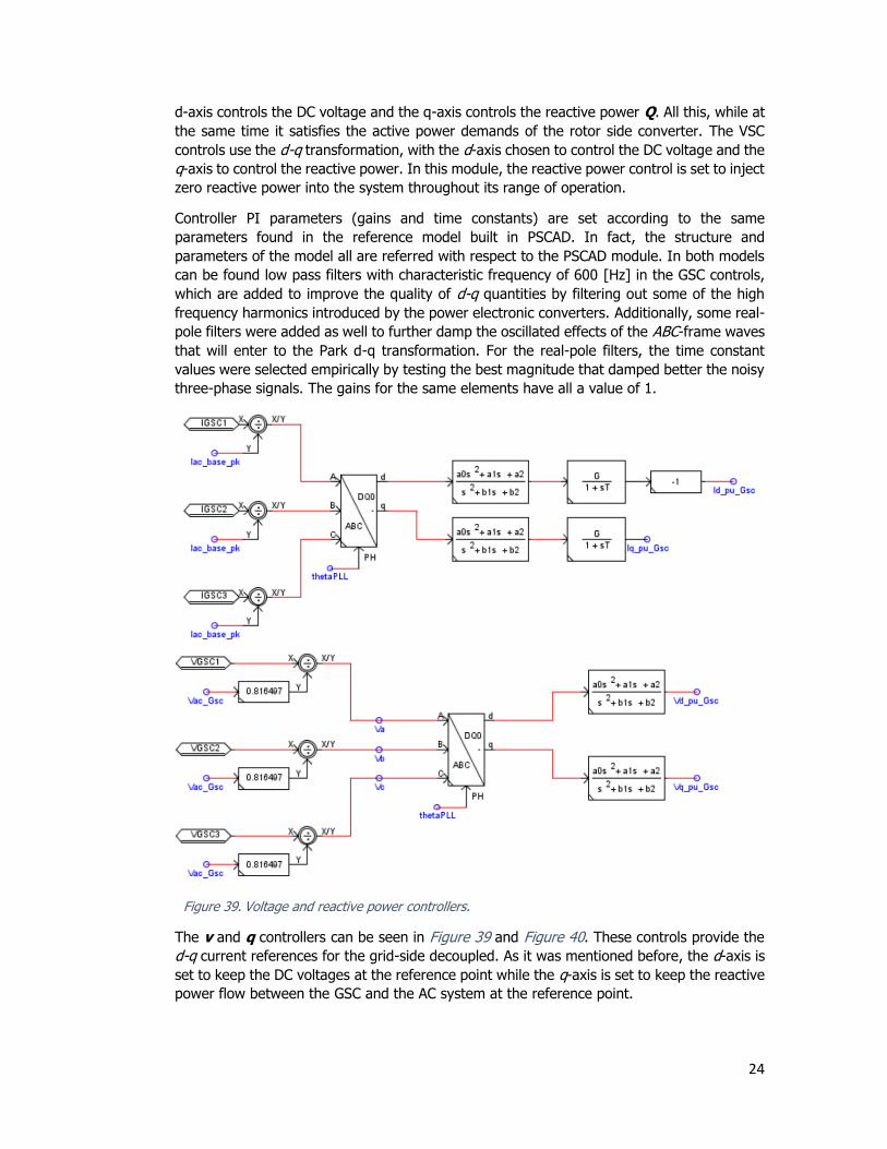
d-axis controls the DC voltage and the q-axis controls the reactive power Q. All this, while at
the same time it satisfies the active power demands of the rotor side converter. The VSC
controls use the d-q transformation, with the d-axis chosen to control the DC voltage and the
q-axis to control the reactive power. In this module, the reactive power control is set to inject
zero reactive power into the system throughout its range of operation.
Controller PI parameters (gains and time constants) are set according to the same
parameters found in the reference model built in PSCAD. In fact, the structure and
parameters of the model all are referred with respect to the PSCAD module. In both models
can be found low pass filters with characteristic frequency of 600 [Hz] in the GSC controls,
which are added to improve the quality of d-q quantities by filtering out some of the high
frequency harmonics introduced by the power electronic converters. Additionally, some real-
pole filters were added as well to further damp the oscillated effects of the ABC-frame waves
that will enter to the Park d-q transformation. For the real-pole filters, the time constant
values were selected empirically by testing the best magnitude that damped better the noisy
three-phase signals. The gains for the same elements have all a value of 1.
The v and q controllers can be seen in Figure 39 and Figure 40. These controls provide the
d-q current references for the grid-side decoupled. As it was mentioned before, the d-axis is
set to keep the DC voltages at the reference point while the q-axis is set to keep the reactive
power flow between the GSC and the AC system at the reference point.
Figure 39. Voltage and reactive power controllers.
25
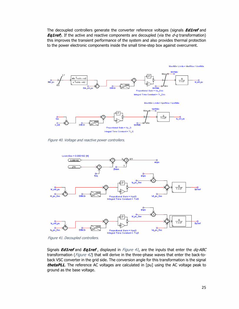
The decoupled controllers generate the converter reference voltages (signals Ed1ref and
Eq1ref). If the active and reactive components are decoupled (via the d-q transformation)
this improves the transient performance of the system and also provides thermal protection
to the power electronic components inside the small time-step box against overcurrent.
Signals Ed1ref and Eq1ref , displayed in Figure 41, are the inputs that enter the dq-ABC
transformation (Figure 42) that will derive in the three-phase waves that enter the back-to-
back VSC converter in the grid side. The conversion angle for this transformation is the signal
thetaPLL. The reference AC voltages are calculated in [pu] using the AC voltage peak to
ground as the base voltage.
Figure 40. Voltage and reactive power controllers.
Figure 41. Decoupled controllers.

26
Rotor-side converter controls. Hierarchical box shown in Figure 43. The rotor-side converter
injects the required currents in the d-q axes by determining the rotor position (slip angle)
with respect to the stator flux in the induction machine, such that the desired conditions of
p and v or q are obtained at the terminals of the machine.
The base quantities for the rotor side converter controls and maximum converter currents
are based on the voltage on the rotor side, which is calculated with the rotor/stator turns
ratio and maximum slip of the induction machine. The magnetizing current is neglected.
As in a similar fashion as with the GSC controls, the rotor currents are also transformed into
the d-q frame. The d-axis currents produce a flux at right angles to this vector, q-axis currents
produce a flux in the air gap that aligns with the rotating flux vector. In this manner, the d-
Figure 43. Rotor-side converter control box.
Figure 42. dq-ABC transformation of the GSC.
27
current component contributes to the torque, while the q-current component contributes to
the reactive power q. Therefore, the stator p and q values can be controlled by controlling
the d-q currents of the rotor.
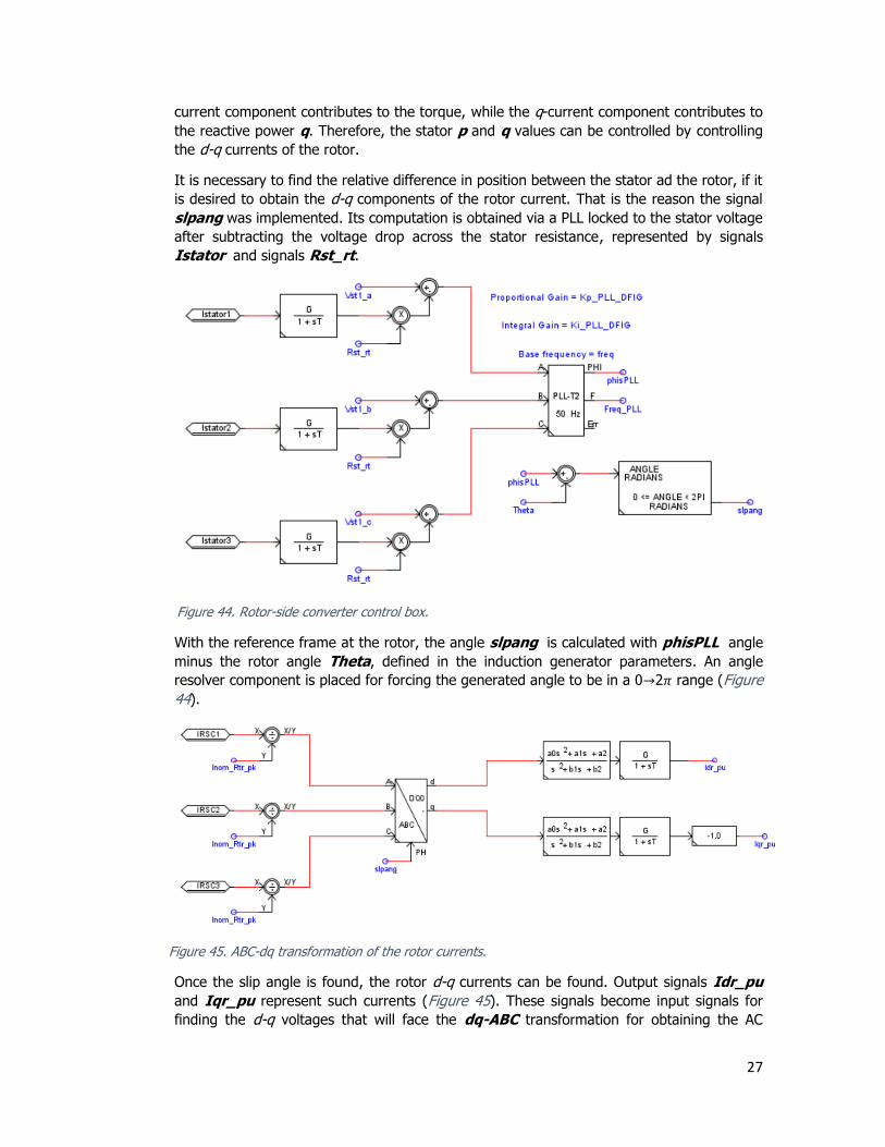
It is necessary to find the relative difference in position between the stator ad the rotor, if it
is desired to obtain the d-q components of the rotor current. That is the reason the signal
slpang was implemented. Its computation is obtained via a PLL locked to the stator voltage
after subtracting the voltage drop across the stator resistance, represented by signals
Istator and signals Rst_rt.
With the reference frame at the rotor, the angle slpang is calculated with phisPLL angle
minus the rotor angle Theta, defined in the induction generator parameters. An angle
resolver component is placed for forcing the generated angle to be in a 0→2𝜋 range (Figure
44).
Once the slip angle is found, the rotor d-q currents can be found. Output signals Idr_pu
and Iqr_pu represent such currents (Figure 45). These signals become input signals for
finding the d-q voltages that will face the dq-ABC transformation for obtaining the AC
Figure 44. Rotor-side converter control box.
Figure 45. ABC-dq transformation of the rotor currents.

28
voltages that enter the VSC converter on the RSC. The signals that enter the dq-ABC
transformation are vdref_pu and vqref_pu. Figure 46 shows the control scheme that the
rotor d-q currents
and voltages once the synchronization process has occurred. The loop containing the signal
vdref_st_pu and the PI controller help the system to have a smooth transition between
controllers before, during and after the synchronization stage occurs.
Crowbar protection. Hierarchical box shown in Figure 47. The crowbar protection is there to
assure that the aerogenerators remain connected to the grid despite any disturbance in the
grid. In case of disturbances, the overcurrent generated may have a dangerous negative
effect on the rotor. As a standard way, wind turbines with the DFIG configuration have their
stator connected to the grid. This makes the rotor winding sensitive to high currents induced
during grid disturbances and faults, like the eleven type-faults also included in this model.
The rotor windings are connected to the grid through the VSC back-to-back converter, which
is very sensitive to overcurrents. The most common means to avoid injecting such induced
currents into the power electronic converters is the use of the aforementioned crowbar, which
shorts the rotor terminals through a resistance.
Figure 47. Crowbar control box.
Figure 46. Rotor-side converter dq voltages with their control schemes.
29
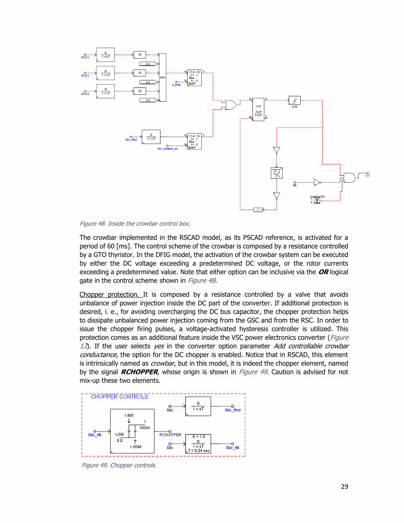
The crowbar implemented in the RSCAD model, as its PSCAD reference, is activated for a
period of 60 [ms]. The control scheme of the crowbar is composed by a resistance controlled
by a GTO thyristor. In the DFIG model, the activation of the crowbar system can be executed
by either the DC voltage exceeding a predetermined DC voltage, or the rotor currents
exceeding a predetermined value. Note that either option can be inclusive via the OR logical
gate in the control scheme shown in Figure 48.
Chopper protection. It is composed by a resistance controlled by a valve that avoids
unbalance of power injection inside the DC part of the converter. If additional protection is
desired, i. e., for avoiding overcharging the DC bus capacitor, the chopper protection helps
to dissipate unbalanced power injection coming from the GSC and from the RSC. In order to
issue the chopper firing pulses, a voltage-activated hysteresis controller is utilized. This
protection comes as an additional feature inside the VSC power electronics converter (Figure
13). If the user selects yes in the converter option parameter Add controllable crowbar
conductance, the option for the DC chopper is enabled. Notice that in RSCAD, this element
is intrinsically named as crowbar, but in this model, it is indeed the chopper element, named
by the signal RCHOPPER, whose origin is shown in Figure 49. Caution is advised for not
mix-up these two elements.
Figure 49. Chopper controls.
Figure 48. Inside the crowbar control box.

30
IEC control. Control scheme structure shown in Figure 50. It is the link between all the
different components of the WTG model. It is based on the IEC 61400 International Standard
published by the International Electrotechnical Commission regarding wind turbines. This
standard ensures that wind turbines are appropriately engineered against damage from
hazards within the planned lifetime. In this scenario the elements being tested have to do
with the turbine components. As inputs it has all electric reference values (f, v, p, q), the
signal that determines (de)-activation of the synchronizer block, and the (de)-activation of
the wind park. Its output wirelabels are the pitch angle control of the blades of the turbine,
and the reactive and active power of the rotor side which are controlled by the rotor d-q
currents.
This sub-system is the most complex of all the subsystems in the model, as it relates signals
from both the mechanical and electrical system and all the previous control schemes. As
mentioned, its input signals embody wirelabels from the GSC controls, meters, the mechanical
power system and the synchronization process, while its output signals are related to the
RSC controls and the mechanical power control system too. It is composed by twelve
hierarchical modules, which are the following:
• Wind power calculation (input choice-back calculation)
• Available power calculation
• Active power reference setpoint
• Reactive power reference setpoint
• Emulation of inertia for the generator
• Angle position (delta) control for the blades
• Reduction of input power
• Q-limits for active power and voltage
Figure 50. IEC 61400 standard control scheme containing all of its hierarchical boxes.

31
• Active power controls
• Reactive power controls
• Current limiter
• Pitch angle control
Wind power calculation (input choice-back calculation). Hierarchical box shown in Figure 51.
This block provides the option of either using the measured wind speed in the model or to
go back and calculate the wind speed from a custom-made equation enclosed in a hierarchical
model inside this box, whose name is WIND POWER EQUATION. The switch that selects
either option has the name Minput. The option enabled by default is taking the measured
wind speed of the model.
Available power calculation. Hierarchical box shown in Figure 52. This module determines the
maximum amount of available power based on the wind speed and on the assumption that
the pitch angle is zero (before the synchronization sequence). This is done via a custom-
component named X to the power of Y, whose output is delayed and filtered in order to
match the reaction time of the related controllers and the damping effect of the turbine.
Active and reactive power reference setpoints. Hierarchical box shown in Figure 53. These
modules relate the management of the active and reactive power generated by the wind
turbine and its incorporation in the wind farm. Signals pPDrefcom and xpPDrefcom are
two of the output signals of the wind farm control. If the wind farm is active, these two
signals are two of the inputs of the p and q controls of the IEC controls subsystem,
respectively.
Figure 51. Input choice-back calculation.
Figure 52. Available power calculation.
Figure 53. Active/reactive power reference setpoints.
32
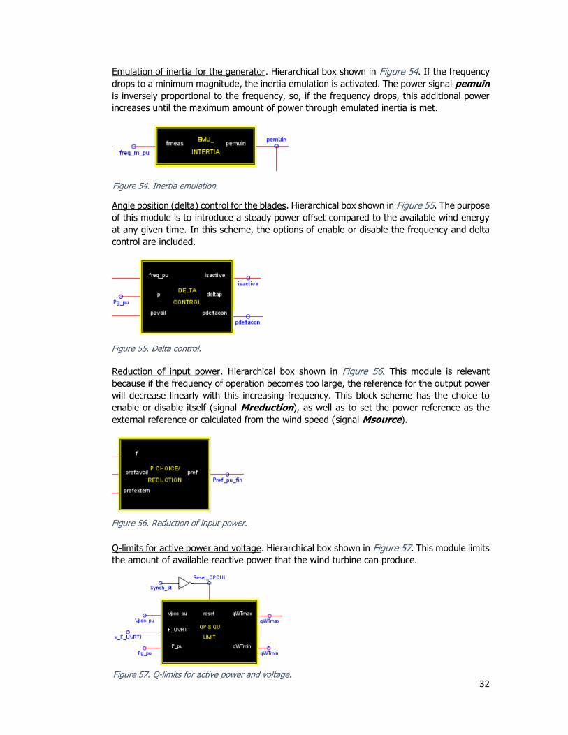
Emulation of inertia for the generator. Hierarchical box shown in Figure 54. If the frequency
drops to a minimum magnitude, the inertia emulation is activated. The power signal pemuin
is inversely proportional to the frequency, so, if the frequency drops, this additional power
increases until the maximum amount of power through emulated inertia is met.
Angle position (delta) control for the blades. Hierarchical box shown in Figure 55. The purpose
of this module is to introduce a steady power offset compared to the available wind energy
at any given time. In this scheme, the options of enable or disable the frequency and delta
control are included.
Reduction of input power. Hierarchical box shown in Figure 56. This module is relevant
because if the frequency of operation becomes too large, the reference for the output power
will decrease linearly with this increasing frequency. This block scheme has the choice to
enable or disable itself (signal Mreduction), as well as to set the power reference as the
external reference or calculated from the wind speed (signal Msource).
Q-limits for active power and voltage. Hierarchical box shown in Figure 57. This module limits
the amount of available reactive power that the wind turbine can produce.
Figure 54. Inertia emulation.
Figure 55. Delta control.
Figure 56. Reduction of input power.
Figure 57. Q-limits for active power and voltage.
33
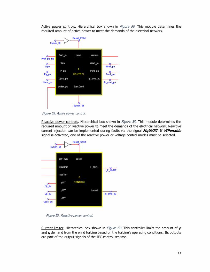
Active power controls. Hierarchical box shown in Figure 58. This module determines the
required amount of active power to meet the demands of the electrical network.
Reactive power controls. Hierarchical box shown in Figure 59. This module determines the
required amount of reactive power to meet the demands of the electrical network. Reactive
current injection can be implemented during faults via the signal MqUVRT. If WPenable
signal is activated, one of the reactive power or voltage control modes must be selected.
Current limiter. Hierarchical box shown in Figure 60. This controller limits the amount of p
and q demand from the wind turbine based on the turbine’s operating conditions. Its outputs
are part of the output signals of the IEC control scheme.
Figure 58. Active power control.
Figure 59. Reactive power control.

34
Pitch angle control. Hierarchical box shown in Figure 61. This module sets the pitch angle
based on the turbine’s power and speed requirements. Its output signal is interdependent
with the calculated wind speed signal Wpu. The output signal is part of the output signals of
the IEC control scheme.
All the mentioned schemes and control systems were designed or taken from the RSCAD
master library. The followed philosophy for the construction of the translated PSCAD model
into RSCAD was to keep it as similar as possible in structure and likeness to the original
model, in order to be easy to any user to identify the similar structures and components
between the two models. That also applied for the names of all signals in the PSCAD model.
The same names were used for all signals in the RSCAD model. The RSCAD model also
includes custom components. PSCAD had several of these components in its control systems.
Along the IEC controls there were several formulas translated into control orders to tune the
reactive/active power and pitch angle, input wirelabel of the rotor-side converter. As
mentioned before, there was custom components in the subsystem defining the wind velocity
and mechanical power from the wind.
Figure 60. Current limiter.
Figure 61. Pitch angle control.

35
2. Debugging compilation errors on draft canvas in RSCAD
After finishing the graphical building of the electric circuits and all the control schemes that represent
the wind turbine model, the draft must face several tests that verifies whether the model is properly
composed or not. The compilation tool (Figure 63) ensures that there are no numerical errors,
impossible tasks in the control scheme orders and/or wrongful electric circuit schemes. If the
compilation window shows no errors, that means the built draft should be ready to run-in a
simulation.
This stage took much time because of the extensive size of the original model. The building process
should be done by hand. Therefore, computation errors arose if parts of the model were not properly
built. That was indeed the case several times. This brought several compilation tests that often
yielded in windows similar to the one shown in Figure 62 announcing compilation errors. The task
of re-drafting a model that executes a control scheme with a given logic in an original software is
usually quite different from the other software where the model is going to be implemented. That
was indeed the case with the translation from PSCAD to RSCAD. Later on, the philosophy or building
the RSCAD model as closest as possible in the structure and logic of PSCAD’s brought more issues in
the runtime simulation tests stage.
3. Test of each sub model that composes the Type-3 Model drafted in RSCAD
This part was done with the objective of demonstrate the correct validation of each sub-system by
parts. This was done by having the reference plots and signals from PSCAD representing a specific
part of the model that was going to be tested. Then, comparing such reference to the built respective
similar part in RSCAD. If both models were having the same input signal values, that means the
Figure 62. Successful compilation of Model
Figure 63. RSCAD draft compilation button

36
output signal and plots should behave similarly in both PSCAD and RSCAD. This part was successful
in several tests conforming each part of the Type-3 Model. Figure 64 shows an example of a test of
an element that takes part of the Type-3 model. There are two plots, showing similar behaviour. This
kind of validation was repeated for each element built separately. Some tests, however, were not
that accurate because in more than once case, sub-systems had variable input signals, difficult to
recreate, also not very worthwhile to spend time in recreating such variable behaviours for each case
with such scenario. For those cases was chosen to select the (variable) input value that lasted the
most within all their variable values in a run (their wirelabel values when if steady-state conditions).
The time invested in this task was also large, since most of the cases, the plots were not giving the
same responses. Therefore, additional debugging had to be done to correct any error that was
preventing to the RSCAD plots to deliver similar performance as the plot signals in PSCAD. Figure 64
shows the control schemes of the grid currents from their sinusoidal three-phase stage to the dq-
transformation domain. The control scheme for RSCAD had two additional real-pole filters for forcing
the output signal to have a straight-line behaviour. More than once that approach had to be
implemented, making tricks to force the wirelabels to present expected performances. That is just
one example, but the in the RSCAD model can be found structures with additional components for
aiding all sub-systems to perform properly.
Figure 64. Successful tests of some components of the Type-3 Model vs. PSCAD similar.
37
4. Integration of all the elements of the model into one big model
Before this part, all individual components were having steady-state-condition input signals
representing the expecting numerical values as it is done in the PSCAD model for each subsystem.
This stage relates and connects all such sub-systems of the model with their corresponding input-
output wirelabels. The outcome is the accommodation of all the sub-systems (all the pieces of the
puzzle) and thus, obtaining the total structure of the system. That is, the realisation of the whole
translation of the Type-3 WTG model from PSCAD into RSCAD. Double-check of the names of each
of all the wirelabels was done to assure that the correct values reach the desired destinations for
complete all the sequences of all control schemes for having a robust model (signal linking
implementation). PSCAD software does not have conflict in having different names for a particular
wirelabel. That is important if given signal is the input (father) for several other different signals
(input repetitions). Once a given signal is defined in its PSCAD Workspace database, that signal will
be the same even if in one of its repetitions has a different name from the one of its origin. RSCAD
software does not have that feature. That feature cannot be replicated in RSCAD. If one wirelabel
was defined with a name, that name must be the same for the repetition of that same signal if it
happens to be the input (father) for other control schemes. Keeping track of all different signals in
the PSCAD model and mimic all the same wirelabels, while also minding the different characteristic
of the signals in RSCAD was the task at this stage.
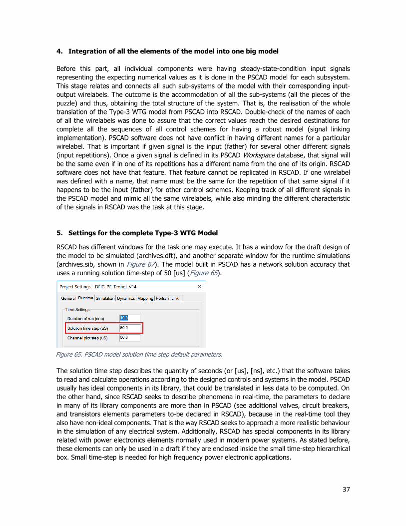
5. Settings for the complete Type-3 WTG Model
RSCAD has different windows for the task one may execute. It has a window for the draft design of
the model to be simulated (archives.dft), and another separate window for the runtime simulations
(archives.sib, shown in Figure 67). The model built in PSCAD has a network solution accuracy that
uses a running solution time-step of 50 [us] (Figure 65).
The solution time step describes the quantity of seconds (or [us], [ns], etc.) that the software takes
to read and calculate operations according to the designed controls and systems in the model. PSCAD
usually has ideal components in its library, that could be translated in less data to be computed. On
the other hand, since RSCAD seeks to describe phenomena in real-time, the parameters to declare
in many of its library components are more than in PSCAD (see additional valves, circuit breakers,
and transistors elements parameters to-be declared in RSCAD), because in the real-time tool they
also have non-ideal components. That is the way RSCAD seeks to approach a more realistic behaviour
in the simulation of any electrical system. Additionally, RSCAD has special components in its library
related with power electronics elements normally used in modern power systems. As stated before,
these elements can only be used in a draft if they are enclosed inside the small time-step hierarchical
box. Small time-step is needed for high frequency power electronic applications.
Figure 65. PSCAD model solution time step default parameters.
38
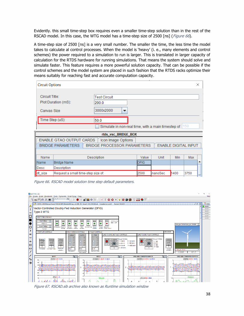
Evidently. this small time-step box requires even a smaller time-step solution than in the rest of the
RSCAD model. In this case, the WTG model has a time-step size of 2500 [ns] (Figure 66).
A time-step size of 2500 [ns] is a very small number. The smaller the time, the less time the model
takes to calculate al control processes. When the model is ‘heavy’ (i. e., many elements and control
schemes) the power required to a simulation to run is larger. This is translated in larger capacity of
calculation for the RTDS hardware for running simulations. That means the system should solve and
simulate faster. This feature requires a more powerful solution capacity. That can be possible if the
control schemes and the model system are placed in such fashion that the RTDS racks optimize their
means suitably for reaching fast and accurate computation capacity.
Figure 67. RSCAD.sib archive also known as Runtime simulation window
Figure 66. RSCAD model solution time step default parameters.

39
Figure 68. RTDS digital system at EWI faculty.
The RTDS system at TU Delft (Figure 68) consists of eight racks. Each rack is composed of 3 to 5
processor electronic cards which are the elements that execute the computations of all runs. TenneT
TSO GmbH has rack #3 reserved for its several research projects related with real-time simulation.
This rack is the one also often used for this project.
For reaching the goal of the 50 [us] and 2500 [ns] time steps, rack #3 had to be upgraded with an
additional processor card for having more power. Another task to achieve the desired solution time
was to place all the relevant control and electric components of the model evenly between the five
cards that conform the rack #3. Controls processors shown in Figure 7 help to do so. The
accommodation of each element to a processor had to be done manually element by element. Most
software packages optimize their resources in an automatic way, unfortunately that is not the case
with RSCAD. The processor assignment of all the elements of the model are shown in Figure 69.
Figure 69. Processor assignment
40
6. Project Outcome: Test and validation of the Type-3 WTG Model
Once the model was completely built, the validation tests of the system were done. The model can
be defined as successfully functional if it reaches the goal of feeding the electric power network
(represented by the 33 [kV] source) with around 3 [MW] of power (around 1 [pu]) or beyond, while
maintaining realistic magnitudes and curves in its other signals. For instance, the PWM voltage signals
that enter-exit the power-electronic VSC from the small time-step box, should also maintain a
sinusoidal shape with amplitudes of around 1 [pu] as well. Additionally, the signal that represents the
aerogenerator pitch angle should be in accordance with the given wind speed input signal, and so
does the mechanical power output signal. For instance, if the input wind speed is around 4 [m/s],
their pitch angle and mechanical power should have magnitudes close to zero.
Exists major differences between the logics of RSCAD and PSCAD software, that must be minded for
assure the suitable performance of the replication of the wind power system model.
When starting this stage, empirically was found out that the logic structure of the PSCAD software
differ significantly from the implemented logic in the RSCAD software. This fact was found out after
doing the first tests and realizing that many of the signal plots were not breeding the same curves
and magnitudes even though, in appearance, both models form PSCAD and RSCAD had the same
structure and initial input values. In conclusion, what in PSCAD means 1, not necessarily also means
1 for RSCAD. The philosophy of built the control logic structures in the RSCAD model according to
PSCAD’s logic is fine in order to keep up and relate similar sub-systems between the models and to
understand the logic of the desired performances of each sub-system, but is recommended to study
the PSCAD and RSCAD manuals for each component used in the system to identify differences in the
operation and logic of the similar components in their different PSCAD and RSCAD versions.
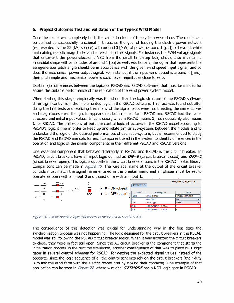
One essential component that behaves differently in PSCAD and RSCAD is the circuit breaker. In
PSCAD, circuit breakers have an input logic defined as ON=0 (circuit breaker closed) and OFF=1
(circuit breaker open). This logic is opposite in the circuit breakers found in the RSCAD master library.
Comparisons can be made in Figure 70. The wirelabel name at the output of the circuit breaker
controls must match the signal name entered in the breaker menu and all phases must be set to
operate as open with an input 0 and closed on a with an input 1.
The consequence of this detection was crucial for understanding why in the first tests the
synchronization process was not happening. The logic designed for the circuit breakers in the RSCAD
model was still following the PSCAD circuit breaker logics. When it was expected the circuit breakers
to close, they were in fact still open. Since the AC circuit breaker is the component that starts the
initialization process in the runtime simulation, another consequence of that was to place NOT logic
gates in several control schemes for RSCAD, for getting the expected signal values instead of the
opposite, since the logic sequence of all the control schemes rely on the circuit breakers (their duty
is to link the wind farm with the electric power grid by closing their contacts). One example of that
application can be seen in Figure 72, where wirelabel S2TMODE has a NOT logic gate in RSCAD.
Figure 70. Circuit breaker logic differences between PSCAD and RSCAD.

41
That was just one main difference besides other crucial ones. For RSCAD machine models, a positive
torque indicates generating operation. For PSCAD it is opposite, as it shown in Figure 71.
In the induction machine for both software tools, there is a switch that defines control by either rotor
speed or rotor torque; the mode depends on a signal integer value. In PSCAD, if the signal is 1, the
machine operates in the speed control mode. In RSCAD, for the machine to also operate in the speed
control mode, that float signal must be 0. After the synchronization process happen, the control mode
both models change from speed to torque. Then, in RSCAD, for the machine to operate in torque
control mode, the signal named S has a value of 1. The different nature in the structure of several
components for each software makes that the plots in some cases vary. One example is shown related
with the dq-reactive components of the ABC-dq transformation for the rotor-side
converter. In any case Both PSCAD/RSCAD WTG models have predetermined the q-component
lagging the d-component of the dq-ABC transformation. This delivers similar plots for each model.
Such phenomenon can be seen in Figure 73, where some of the dq-rotor currents are plotted. All
rotor values are intrinsically related with the induction machine, whose structure varies from software
to software. Rotor-side converter currents in Figure 73 have virtually the same values for both models
built in the two different software packages. Signals named iQ_max, iQ_min, iQ_cmd
(=Iq_cmd_pu) are the input signals of other control schemes whose output signals are rotor voltage
signals vdref_pu and vqref_pu in Figure 74. Despite having the same input values for those control
schemes, the output signals differ in magnitude.
That phenomenon is unwittingly replicated more than once when comparing similar plots coming
from the different models developed in the different software packages. Initially the student tried to
force some of those plots from the RSCAD model to converge to the same values resulted from the
PSCAD reference. This was done by playing with allowable changeable input parameters (i.e., sliders),
use of limiters, real pole and signal filters, but from those experiences the student learnt that the
consequences of using such tools not always gives desirable outcomes. Because of such effects the
student decided to let live some of these odd effects in the simulation and study the behaviour of the
most important plots.
Figure 71. Generation mode differences between RSCAD and PSCAD configurations
Figure 72. Speed-torque control mode differences between RSCAD and PSCAD configurations

42
Figure 73. PSCAD Plots and control schemes of rotor-side currents and voltages. The equivalent components converted into RSCAD.

43
After studying some of the most important control signals, was found that despite some signals that
take part of the whole sequence of the system behave odd, that does not affect in the main objective
of the wind power system, which is deliver active power P from the wind to the electrical network.
After such differences were corrected, the simulation results started to converge similar plots
compared to its PSCAD reference. There were still however some wirelabels that did not plot
reasonable performances, the aerogenerator blades pitch angle being one, the calculated wind speed
being other and the PWM rotor-side converter AC voltages plot being another response that was
breeding erratic plots.
The errors in the pitch angle and the wind speed wirelabel values were corrected once the differences
between speed-to-torque control modes and generation-motoring differences in the induction
machine between PSCAD and RSCAD were detected and corrected. However, the pitch angle was
still having wrongful signal values during minimum conditions. That performance was later detected
because of the output wirelabel of the electric power order when the switch in charge of (de)activate
the wind farm was OFF.
As for the PWM rotor-side converter AC voltages, if the wind speed input parameter is low, the rotor-
side converter AC voltages get a lower frequency, making the sinusoidal shapes to extend. This effect
happens because since the aerogenerator rotor blades rotate periodically less, the sinusoidal waves
take more time to finish one period or oscillation. The error there was that in some cases, especially
if when the parameter input controls were changed very drastically, the AC rotor voltages resulted in
stretched sinusoidal curve, sometimes so stretched that stopped to have an oscillatory sinusoidal
behaviour to now have a DC behaviour. This effect was mitigated after adding some signal selectors
in the outcome of the signal Pord_pu. However, it is still recommended not-to change drastically
the parameter input controls. While the lower-period sinusoidal waves were an acceptable
consequence, the DC curves were not. The reason this effect happened was because in the ABC-dq
transformation stage of the rotor currents, some real-pole filters were added to force the dq-currents
plot straight lines, as it should be according to the direct-quadrature-zero transformation states. The
time-constants set in these real-pole filters were matching cut-off frequency parameters inside the
second-order complex pole filters already placed in the Idr_pu and Iqr_pu rotor dq-currents (in the
Figure 74. Plots of rotor-side current voltages.

44
RSC controls, these filters have a cut-off frequency of 500 [Hz]), as seen in Figure 73. These current
signals are related with the rotor dq-voltages that later experiment a counter-respective dq-ABC
transformation; the obtained three-phase outputs are the aforementioned rotor-side converter PWM
AC voltages. This undesirable effect was mitigated by placing other real-pole filters, this time with
time-constant values opposite to the ones placed during the ABC-dq rotor currents transformation.
These real-pole filters can also be found in Figure 73 in the RSCAD control schemes that have as
outputs the wirelabels vdref_pu and vqref_pu.
The most important plots/controls signals are the ones that show the health of the wind power
system. If these plots are healthy, this could mean that the wind power system is dispatching active
power to the electrical network that is connected to the wind farm, while minding maintaining a
suitable dynamic behaviour of the machine and a decent harmonic behaviour of the converter. The
power rating of the machine is 3.6 [MW] (4 [MVA]). This means that if the active power delivered to
the grid is around these units, the wind power system is doing its job.
Moreover, if the machine is delivering around 3.6 [MW] and the output wirelabels form the IEC control
scheme have similar values compared to the PSCAD wind power system model, and the AC voltages
that enter the DC VSC converter are also equivalent to the respective signals in the PSCAD model,
the RSCAD wind power system model is functional.
Issues involving the PSCAD model
When running simulations with minimum input conditions (wind speed of around 3 [m/s] and/or only
one wind turbine activated), was found that the system fails to provide active power to the grid. On
the contrary, it consumes active power, acting exactly the opposite way as it should be acting. This
effect also was found in the PSCAD model when running a simulation under same initial conditions
(Figure 75). That performance happens because, according to the six mono-phase VSC small time-
step interface transformers (Figure 11), the power electronics converter needs a minimum active
power of 1.494 [MVA] to work. Power losses can also be found in the three-phase transformer, the
induction machine and in the machine scaling circuit. Therefore, the wind power system model has
to at least produce amount of power equivalent to all the system losses for actually not provide any
[MW] but not consuming either.
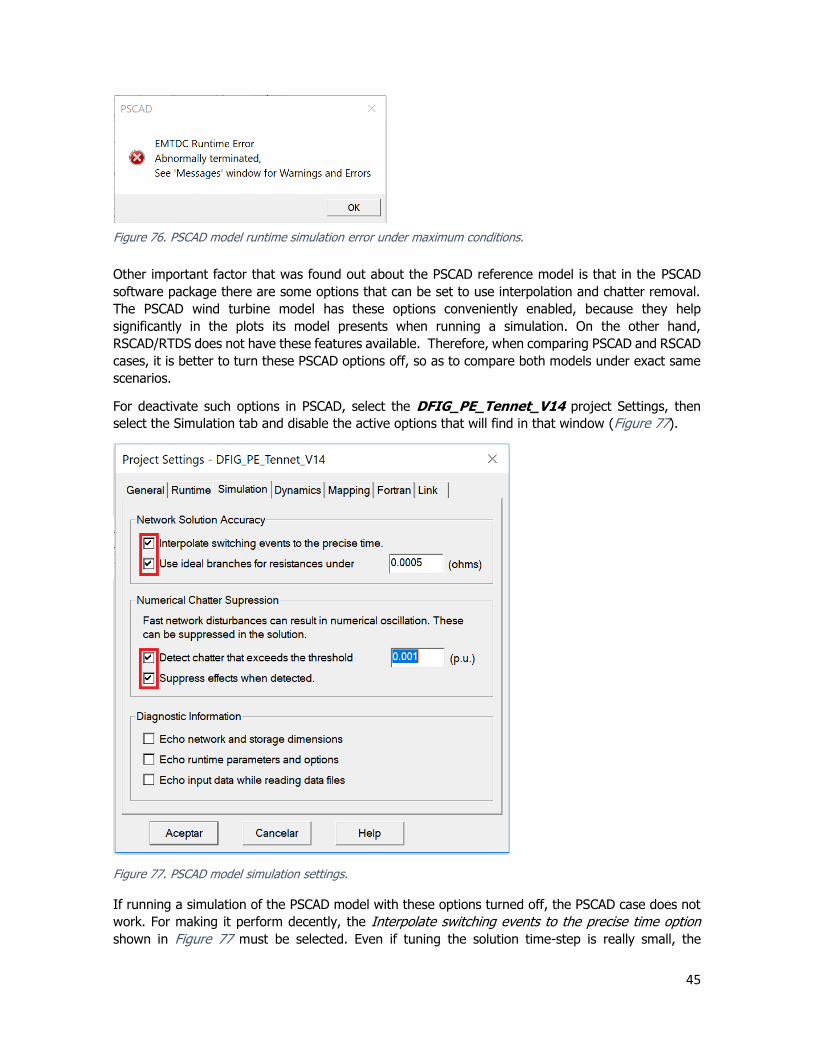
It was also found out that the PSCAD model unable to perform a 10 [s] simulation under maximum
initial conditions (wind speed of around 25 [m/s] and/or one hundred wind turbines activated). After
around 5 [s], the simulation presents an EMTDC runtime error with an abnormal performance of the
induction machine (see Figure 76). Under the same conditions, the RSCAD model is capable of
running a simulation without stop.
Figure 75. Active power in [MW] under minimum conditions in the PSCAD model.
45
Other important factor that was found out about the PSCAD reference model is that in the PSCAD
software package there are some options that can be set to use interpolation and chatter removal.
The PSCAD wind turbine model has these options conveniently enabled, because they help
significantly in the plots its model presents when running a simulation. On the other hand,
RSCAD/RTDS does not have these features available. Therefore, when comparing PSCAD and RSCAD
cases, it is better to turn these PSCAD options off, so as to compare both models under exact same
scenarios.
For deactivate such options in PSCAD, select the DFIG_PE_Tennet_V14 project Settings, then
select the Simulation tab and disable the active options that will find in that window (Figure 77).
If running a simulation of the PSCAD model with these options turned off, the PSCAD case does not
work. For making it perform decently, the Interpolate switching events to the precise time option
shown in Figure 77 must be selected. Even if tuning the solution time-step is really small, the
Figure 76. PSCAD model runtime simulation error under maximum conditions.
Figure 77. PSCAD model simulation settings.

46
interpolation should not be a significant factor. However, even under that scenario, the PSCAD case
still does not work. Furthermore, if the option Supress effects when detected for chatter suppression
is turned OFF, can be seen that the waveforms in the PSCAD model are not as clean as if that option
is enabled. In conclusion, when the comparison stage between the model cases of PSCAD and RSCAD,
it is very recommended to turn OFF these PSCAD settings that, otherwise ON, pull an advantageous
performance with respect to the RSCAD model case, which may not be fair because RSCAD does not
have such features that allow its plots to pretty up. The student working in this internship
unfortunately realized quite late about these PSCAD features that in the DFIG_PE_Tennet_V14
project case in mint -condition were activated. The PSCAD vs. RSCAD plots tests that are shown later
in this document present PSCAD’s with these features ON.
Validation stage
Results of the final tests confirmed that the wind power system built in RSCAD succeeds in feeding
the grid with active power with around 1 [pu] when the input parameters are properly tuned. The
model includes the input signals of the given wind speed, which can be variated with a slider with
minimum/maximum limits of 3-to-25 [m/s] (10.8-to-90 [km/h]). The other variable input is the
number of active wind turbine generators. This input is directly related to the scaling factor. The
RSCAD wind power system model has also to stay robust with different input parameters. The default
initial working conditions in the PSCAD model has 10.2 [m/s] (37 [km/h]) and 50 active wind turbines.
The system works steadily fine if the wind speed input parameters are between 7 to 20 [m/s]. If the
wind park is disabled, it is recommended to leave the slider of the active wind turbines with only one
unit active. If the wind park is active, the model works steadily fine if the number of active
aerogenerators are between 20 to 70. Under these input parameters, the wind farm successfully
feeds active power to the grid. While it does so, the model is robust and stays controlled regardless
of any input initial parameter conditions. Also, when simulating any of the 11 types of faults, the
system stays robust. Tests were done to validate the model in very harsh conditions (varying winds
from very low to very high speeds and at the same time, increase/decrease dramatically the number
of active aerogenerators). One issue to-be improved is that, outside the recommended input
parameters, the model struggles to maintain dynamic/harmonic stability. When running simulations
under extreme conditions, the model still performs positively, but this not always happen.
Additionally, ripple and deformed oscillations appear in most of the plots. These effects increase when
increasing the scaling factor. Also, when trying to change input parameters too drastically and
extremely, the model may take time to get back control or lose it, but that is also the case with the
PSCAD WTG model. When comparing the model to the one built in PSCAD, not all the plots behave
100% to this reference; but all of them follow the expected performance and behaviour of the power
wind farm under recommended input conditions.
The RSCAD model must work without problems in such conditions, but must work correctly too if the
wind speed is not strong (3 [m/s]). Under that condition may not be suitable to leave active 50 WTGs,
perhaps one single units if fine, since in that case the wind speed is low. Therefore, the model must
respond well in such scenario. Same if the wind is blowing very strongly. In that case the model was
tested on maximum conditions (25 [m/s] and 100 active units) to validate if the system keeps
working. Lastly, the RSCAD model must to stay robust under all already stated scenarios and if any
transient or fault suddenly occurs. The model must feel the fault, but after instants, should be capable
of maintain the stability of the system despite all the entropic phenomena. All plots are important to
study and verify to know if the system is working properly and is in a healthy state, but the ones that
define decent performance are the following:
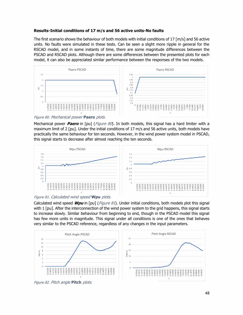
• Mechanical power Paero in [pu]. Power that is a consequence of the strength of the wind,
and responsible for the (electric) torque of the induction machine.

47
• Calculated wind speed Wpu in [pu]. This signal recalculates the wind speed after the
synchronization sequence has taken place.
• The pitch angle of the WTG blades Pitch in [pu]. This angle is a consequence of the strength
of the wind, and has an interdependence relationship with the signal Wpu.
• Electric power Pord_pu in [pu]. This signal sets the order of delivering active power.
• Current signals iQ_max, iQ_min, iP_max in [pu]. These signals, together with the signal
Pitch, are the outputs of the IEC control scheme that is intrinsically related to the rotor
controls of the electric machine.
• Delivered active power Pg_pu in [pu]. In the beginning of the simulation this signal depends
on the initial conditions to the grid at 33 [kV], after the synchronization sequence has taken
place, will be dependent on all of the above signals for providing active power to the grid.
• Rotor-side VSC converter voltages Vra, Vrb and Vrc in [pu]. AC voltages that enter to the
right-side of the DC power-electronics converter.
• Grid-side VSC converter voltages VrefGSa, VrefGSb and VrefGSc in [pu]. AC voltages that
enter to the left-side of the DC power-electronics converter.
Check the curves and magnitudes of the signals of currents, voltages and PLL radians to be sure that
the system is fine or if it has any malfunction in some part of its structure. Check the synchronization
time. Should not take more than one minute (Figure 79). Other signals that help to verify optimal
condition of the wind power system are:
• Capacitor VSC DC voltage Edc in [pu] and all its derivatives after filtering processes.
• PLL output signals Theta_PCC and thetaPLL (from grid-side converter controls), Theta,
phisPLL and slpang (from rotor-side converter controls), all in [radians]. Wirelabel slpang
is the slip angle after substracting Theta to phisPLL. Most PLL angle plots in both PSCAD
and RSCAD models behave like Theta_PCC plot shown in Figure 78, with vertical lines facing
the right-side of the plot. slpang plot is the only PLL plot that has an opposite behaviour,
having the same vertical component facing the left-side of the plot.
For validate the RSCAD model, the plots of the mentioned signals were imported from PSCAD and
RSCAD to Excel under different conditions. The results from the RSCAD model got a leading offset
for matching the time that the PSCAD model completes the synchronization process.
Figure 78. PLL output plots.
Figure 79. Monitoring signals.
48
Results-Initial conditions of 17 m/s and 56 active units-No faults
The first scenario shows the behaviour of both models with initial conditions of 17 [m/s] and 56 active
units. No faults were simulated in these tests. Can be seen a slight more ripple in general for the
RSCAD model, and in some instants of time, there are some magnitude differences between the
PSCAD and RSCAD plots. Although there are some differences between the presented plots for each
model, it can also be appreciated similar performance between the responses of the two models.
Mechanical power Paero in [pu] (Figure 80). In both models, this signal has a hard limiter with a
maximum limit of 2 [pu]. Under the initial conditions of 17 m/s and 56 active units, both models have
practically the same behaviour for ten seconds. However, in the wind power system model in PSCAD,
this signal starts to decrease after almost reaching the ten seconds.
Calculated wind speed Wpu in [pu] (Figure 81). Under initial conditions, both models plot this signal
with 1 [pu]. After the interconnection of the wind power system to the grid happens, this signal starts
to increase slowly. Similar behaviour from beginning to end, though in the PSCAD model this signal
has few more units in magnitude. This signal under all conditions is one of the ones that behaves
very similar to the PSCAD reference, regardless of any changes in the input parameters.
Figure 80. Mechanical power Paero plots.
Figure 81. Calculated wind speed Wpu plots.
Figure 82. Pitch angle Pitch plots.

49
The pitch angle of the WTG blades Pitch (Figure 82) has a higher maximum point for the RSCAD
model. This control scheme is very sensitive to changes and during the validation stage this signal
was the most difficult paramter to make it behave as it should, losing control and reaching its
maximum peak even if the input parameters have miminum conditions. This signal finally converged
to desired values after changing the induction machine model from an ond version inside the small
time-step box to the current one in use, nacem WTG. Aditionally, the control modes logic were
reviewed to validate that the induction machine was indeed working as a generator in torque mode.
In this plot, although intially has a siginificatly large peak compared to the PSCAD value, after ten
seconds both plots converged to closer values in degrees.
Electric power Pord_pu (Figure 83) response comparison for this test was the least similar plot
between the PSCAD and RSCAD models. This, however does not affect the final values after ten
seconds have passed after the start of the running simulation. Both parameters converged to around
1 [pu]. This signal in the RSCAD model does not reach to values larger than 1 [pu] for deliberate
reasons; the output of this signal has a hard limiter with a maximum value of 1. The reason of this
is because if otherwise, and in case the wind park switch (inside the wind park control panel shown
in Figure 96) is OFF, then the pitch angle signal Pitch losses control and reaches 25 degrees, even
though under that scenario, an inactivated wind park would mean that the wind speed is rather low.
Therefore, such limit had to be set, in order to have reasonable responses.
Current signals iQ_max, iQ_min, iP_max performances (Figure 84) for both models are
conveniently similar. It is convenient indeed because these signals, along with Pitch are the output
signals of the IEC 61400 control scheme, which is large in magnitude and complex. All of these
outputs have primary influence on the behaviour of the induction machine.
Figure 83. Electric power Pord_pu plots.
Figure 84. Current signals iQ_max, iQ_min, iP_max plots.
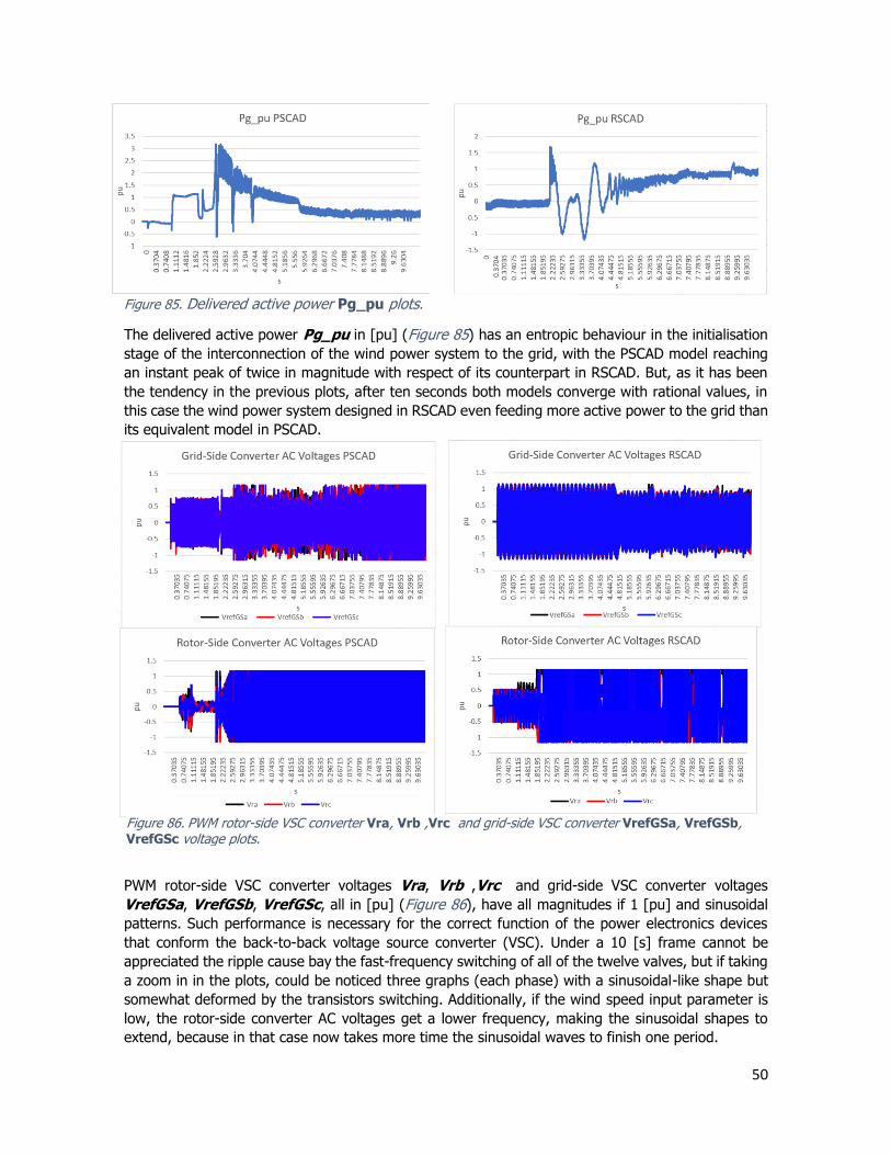
50
The delivered active power Pg_pu in [pu] (Figure 85) has an entropic behaviour in the initialisation
stage of the interconnection of the wind power system to the grid, with the PSCAD model reaching
an instant peak of twice in magnitude with respect of its counterpart in RSCAD. But, as it has been
the tendency in the previous plots, after ten seconds both models converge with rational values, in
this case the wind power system designed in RSCAD even feeding more active power to the grid than
its equivalent model in PSCAD.
PWM rotor-side VSC converter voltages Vra, Vrb ,Vrc and grid-side VSC converter voltages
VrefGSa, VrefGSb, VrefGSc, all in [pu] (Figure 86), have all magnitudes if 1 [pu] and sinusoidal
patterns. Such performance is necessary for the correct function of the power electronics devices
that conform the back-to-back voltage source converter (VSC). Under a 10 [s] frame cannot be
appreciated the ripple cause bay the fast-frequency switching of all of the twelve valves, but if taking
a zoom in in the plots, could be noticed three graphs (each phase) with a sinusoidal-like shape but
somewhat deformed by the transistors switching. Additionally, if the wind speed input parameter is
low, the rotor-side converter AC voltages get a lower frequency, making the sinusoidal shapes to
extend, because in that case now takes more time the sinusoidal waves to finish one period.
Figure 86. PWM rotor-side VSC converter Vra, Vrb ,Vrc and grid-side VSC converter VrefGSa, VrefGSb, VrefGSc voltage plots.
Figure 85. Delivered active power Pg_pu plots.

51
Results-Initial conditions of 17 m/s and 56 active units-Short-Circuit Fault in Phase A-
to-Ground
The second scenario shows the behaviour of both models with initial conditions of 17 m/s and 56
active units. A phase-to-ground short circuit fault was simulated in phase A. The RSCAD wind power
system model can simulate all types of faults from phase-to-ground or phase-to-phase. When testing
any of the faults while a simulation of power delivering is running, the model experiences a transient
fault that instants after will imbalances the curves. This, however, is mitigated seconds after. This
validates that the RSCAD model is robustly stable even if any potential fault occurs.
The six plots shown in Figure 87 are the responses of three different signals in the PSCAD and RSCAD
models.
• Vpcc_pu (pcc stands for ‘point of common coupling’) is the bus voltage that can be
measured in the primary winding of the three-phase transformer, in [pu]. The fault instant
is denoted in the first two plots with a vertical red line.
Figure 87. Results-Initial conditions of 17 m/s and 56 active units- Short-Circuit Fault in Phase A-to-Ground.

52
• Pg_pu and Qg_pu are the active and reactive power dispatched to the grid, they are the
[pu] counterparts of signals PG and QG, in [MW], which are measured by the Multimeter for
BUS 2. The fault instant is denoted in the third and fourth with a vertical blue line.
• Current signals IBA, IBB and IBC in [kA] are the sinusoidal currents related with the 33
[kV] main voltage source. They represent the current status of the grid. The fault instant is
denoted in the fifth and sixth with a vertical green line.
All signals must be monitored during a transient to verify if the system remains robust or suffers
damage after such transient, but these signals are good checkpoints to detect a healthy or defective
state of the system, since Pg_pu represents the power delivered to the grid, and if this signal reads
less power than expected, that means the system is no longer efficient. Similarly, IBA, IBB and IBC
can be useful to read the status of the grid after any transient. If the system is robust, these currents
have to tolerate the surge [kAs] of current generated by hazardous switching, short-circuits or
lightning. The plots should show a big surge current, but instants after that event, the plots should
show a three-phase sinusoidal current with the same amplitude magnitudes before the transient
happened.
Instructions for tuning the model parameters
The wind power system model developed for its use with RTDS/RSCAD has its functional parameters
defined as the same fashion as its reference model developed in PSCAD. This applies universally in
all individual components, filters, transfer functions PIs, gains, time constants, sliders and all
controllers in the model.
In the draft file, where the RSCAD model is sketched, can be found several sliders, for tuning properly
the parameters these sliders are related. If it is desired to change the limits of these sliders, one just
must select the item to be changed, and edit the numbers that appear on the tabs Maximum value
and Minimum value. However, caution to select suitable numbers should be taken, since the numbers
defined in most controls are based on the successful functionality of the PSCAD model. There are
two places where major set of sliders can be found. Inside the DFIG controls hierarchical box, on
the lower-right part of that window, two sections with sliders can be found as seen in Figure 88. One
related to each side of the power electronics converter.
Figure 88. GSC/RSC sliders.
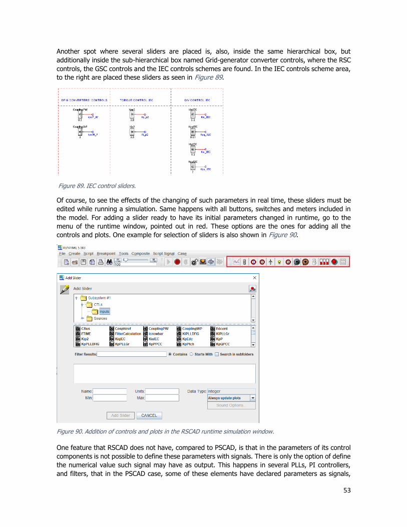
53
Another spot where several sliders are placed is, also, inside the same hierarchical box, but
additionally inside the sub-hierarchical box named Grid-generator converter controls, where the RSC
controls, the GSC controls and the IEC controls schemes are found. In the IEC controls scheme area,
to the right are placed these sliders as seen in Figure 89.
Of course, to see the effects of the changing of such parameters in real time, these sliders must be
edited while running a simulation. Same happens with all buttons, switches and meters included in
the model. For adding a slider ready to have its initial parameters changed in runtime, go to the
menu of the runtime window, pointed out in red. These options are the ones for adding all the
controls and plots. One example for selection of sliders is also shown in Figure 90.
One feature that RSCAD does not have, compared to PSCAD, is that in the parameters of its control
components is not possible to define these parameters with signals. There is only the option of define
the numerical value such signal may have as output. This happens in several PLLs, PI controllers,
and filters, that in the PSCAD case, some of these elements have declared parameters as signals,
Figure 89. IEC control sliders.
Figure 90. Addition of controls and plots in the RSCAD runtime simulation window.

54
normally related with sliders, so these parameters can be variable. One example of this situation is
shown in Figure 91 where a PI controller for the GSC has as input parameters signals from sliders.
This example, in the PSCAD case has the signals enclosed in red defined as parameters for that PI
controller. The exact PI controller in RSCAD has defined the numbers that signals Kp_Q and Ti_Q
have set as default in their sliders. In this case, the limits IqrefMax and IqrefMin are placed outside
the PI controller in order to be able to define them as signals too. The rule of thumb to define if a
controller does not have defined its inputs as variable values is to see if around that element are
comments that state where and how a particular input parameter was declared. Enclosed in green
can be seen the values of the proportional gain and the integral time constant of the PI controller.
RSCAD case also has declared signals Kp_Q and Ti_Q on sliders. However, modifying this signals in
that case will have no effect on the model performance. The idea is that the user pay attention to
these comments, like the ones enclosed in green, so that if the user wants to change the number of
a similar parameter, should go to that slider to take reference of the declared maximum and minimum
feasible values for that parameter. Despite parameters in RSCAD for some elements cannot be
defined as (variable) signals, all of the declared parameters in the PSCAD DFIG_PE_Tennet_V14
case are the values that are considered more suitable for the best performance possible. So, it is
actually not expected to modify the values of such parameters. The idea of having these signals
variable is to have a more-dynamic model, for experiment what would happen if certain parameter
Figure 91. Variable input parameters defined in GSC PI controller in PSCAD/RSCAD cases.

55
suddenly changes. In conclusion, the selected parameters found in the RSCAD model case, are the
same ones found by default in the PSCAD DFIG_PE_Tennet_V14 case in mint-condition.
If a user of the RSCAD wind power system model wants to take reference of any of the defined
parameters of the model, the following tables show the expected values for each. These tables are
same ones found in the model documentation for the PSCAD DFIG_PE_Tennet_V14 case (please,
see reference [5]). These tables are replicated in this document to have ready the references for
each parameter in case the user does not have the PSCAD model documentation available. As stated
before, numbers and parameters found in the PSCAD case are the same ones that will be found in
the RSCAD model case. The signals that appear on the tables with red italics are the one that have
input parameters variable via sliders. Double check is advised to do on these signals in case the user
wants to modify such parameters, because, as explained before, the sliders related to these variable
signals may not actually vary the initial values. Tables retrieved from reference ‘J. C. Garcia, K.
Mudunkotuwa, C. Shumski. Manitoba HVDC Research Centre. DRAFT. Migrate project, Type-3 and
Type-4 EMT model documentation’.
Table 1. DFIG converter parameters
Parameter Unit or
[pu] base Value Description
1. General
Capacitance [µF] 18000 [µF] DC bus capacitance
AC system
frequency
[Hz] 50 [Hz] Nominal AC system frequency
Voltage on high
side of TRF
[kV] 33 [kV] Voltage of the Wind Farm collector system
2. Machine parameters1
System MW at PCC [MW] 3.6 [MW] The expected full active power at the point of common coupling. This
value is used as the base active power Pbase for per-unitization of
quantities
Machine rating [MVA] 4.0[MVA] The MVA rating of the machine. Note that this value should be higher
than the previous one to account for reactive power consumption of
the machine and the converter losses
Machine terminal
voltage
[kV] 0.9 [kV] Nominal voltage of the stator terminals
Stator resistance [pu] 0.005 [pu] Per unit value of the resistance of the stator windings
1 The machine parameters shown here only include the quantities that are also required in the setup of the controls. The full machine parameters still need to be entered in the RSCAD machine
component. For explanation on those parameters please see the Induction Machine component help
in RSCAD [7].

56
Slip_max [-] 0.3 Maximum operating slip of the machine
Stator/Rotor turns
ratio
[-] 0.3 Turns ratio between stator and rotor windings
3. Filter parameters
Cflter [uF] 1466 [uF] Main filter capacitance
Cdamp [uF] 733 [uF] Damping branch capacitance
Ldamp [H] 0.0096 [H] Damping branch inductance
Rdamp [ohm] 1.447 [ohm] Filter’s damping resistance
DC chopper
Activation voltage [kV] 1.65 [kV] Chopper hysteresis control activation voltage
4. OFF voltage [kV]
Shunt resistor [ohm] 1.0 [ohm] Chopper resistance
Crowbar
protection
DC crowbar ON
voltage
[kV] 1.75 [kV] Crowbar activation by DC link overvoltage: Activation voltage
5. Maximum Irotor [kA]
Crow bar
resistance
[ohm] 0.2 [ohm] Crowbar resistance
Crowbar
inductance
[H] 20 [uH] Value or inductance series to crowbar system
Table 2. Initial conditions of the induction machine
Parameter Unit or
[pu] base Value Description
Machine initial
power
[pu] 1.0 [pu] DC bus capacitance
Initial input torque [pu] 1.0 [pu] Nominal AC system frequency
Machine rotating
speed
[pu] 1.0 [pu] Voltage of the Wind Farm collector system
Initial voltage [pu] 1.0 [pu] Initial RMS voltage at PCC
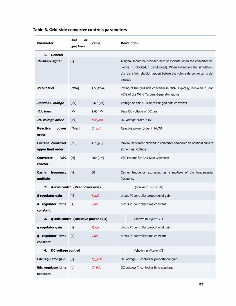
57
Table 3. Grid-side converter controls parameters
Parameter Unit or
[pu] base Value Description
1. General
De-block signal [-] - A signal should be provided here to indicate when the converter de-
blocks. (0:blocked, 1:de-blocked). When initializing the simulation,
this transition should happen before the rotor side converter is de-
blocked
Rated MVA [MVA] 1.5 [MVA] Rating of the grid side converter in MVA. Typically, between 20 and
40% of the Wind Turbine Generator rating
Rated AC voltage [kV] 0.69 [kV] Voltage on the AC side of the grid side converter
Vdc base [kV] 1.45 [kV] Base DC voltage of DC bus
DC voltage order [kV] Edc_ord DC voltage order in kV
Reactive power
order
[Mvar] Q_ord Reactive power order in MVAR
Current controller
upper limit order
[pu] 1.2 [pu] Maximum current allowed in converter compared to nominal current
at nominal voltage
Converter VSC
reactor
[H] 200 [uH] VSC reactor for Grid Side Converter
Carrier frequency
multiple
[-] 60 Carrier frequency expressed as a multiple of the fundamental
frequency
2. d-axis control (Real power axis) (shown in Figure 41)
d regulator gain [-] KpdS d-axis PI controller proportional gain
d regulator time
constant
[s] TidS d-axis PI controller time constant
3. q-axis control (Reactive power axis) (shown in Figure 41)
q regulator gain [-] KpqS d-axis PI controller proportional gain
q regulator time
constant
[s] TiqS d-axis PI controller time constant
4. DC voltage control (shown in Figure 40)
Edc regulator gain [-] Kp_Edc DC voltage PI controller proportional gain
Edc regulator time
constant
[s] Ti_Edc DC voltage PI controller time constant

58
5. Reactive power control
Q regulator gain [-] Kp_Q Reactive power PI controller proportional gain
Q regulator time
constant
[s] Ti_Q Reactive power PI controller time constant
6. PLL control
Ki_PLL_Gr [1/s] Kp_Q Grid side converter PLL integral gain
Kp_PLL_Gr [-] Ti_Q Grid side converter PLL proportional gain
Table 4. Rotor-side converter controls parameters
Parameter Unit or
[pu] base Value Description
1. General
De-block signal [-] - A signal should be provided here to indicate when the converter de-
blocks. (0:blocked, 1:de-blocked). When initializing the simulation,
this transition should happen after the grid side converter is de-
blocked
Rated MVA [MVA] 1.5 [MVA] Rating of the grid side converter in MVA. Typically, between 20 and
40% of the Wind Turbine Generator rating
Rated AC voltage [kV] 0.69 [kV] Voltage on the AC side of the grid side converter
Active power order [pu] Pref_pu Reactive power order in MVAR
Reactive power
order
[pu] Qref_pu Reactive power order in MVAR
Current controller
upper limit order
[pu] 1.2 [pu] Maximum current allowed in converter compared to nominal current
at nominal voltage
Carrier frequency
multiple
[-] 37 Carrier frequency expressed as a multiple of the fundamental
frequency
2. d-axis control for start-up (shown in Figure 46)
Kpd_st (startup) [-] Kpd_st d-axis PI controller proportional gain to be used in the pre-
synchronization phase during start-up
Tid_st (startup) [s] Tid_st d-axis PI controller time constant to be used in the pre-
synchronization phase during start-up
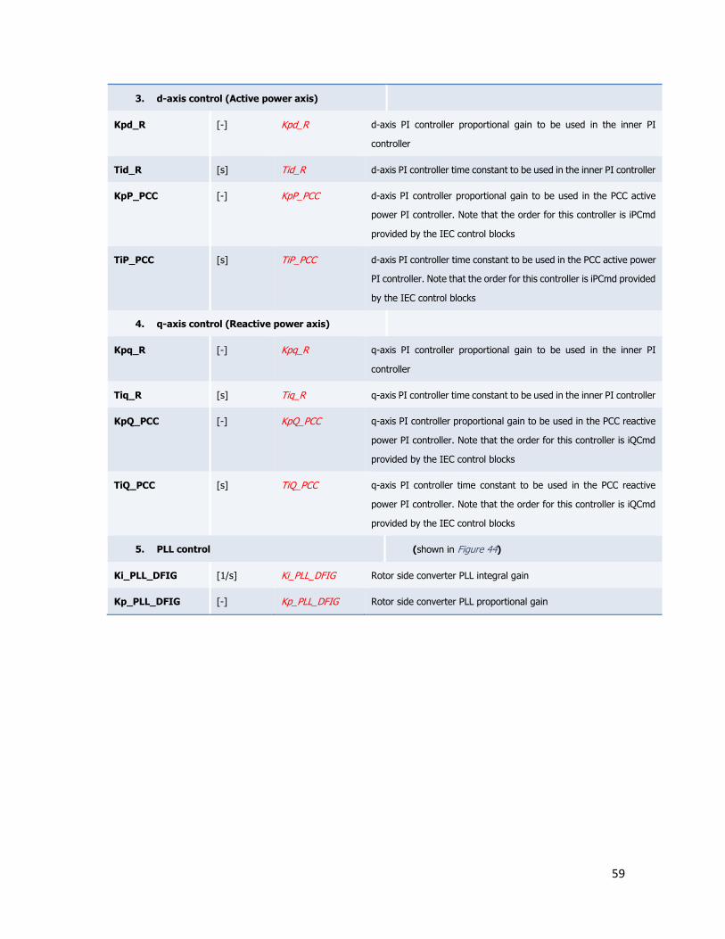
59
3. d-axis control (Active power axis)
Kpd_R [-] Kpd_R d-axis PI controller proportional gain to be used in the inner PI
controller
Tid_R [s] Tid_R d-axis PI controller time constant to be used in the inner PI controller
KpP_PCC [-] KpP_PCC d-axis PI controller proportional gain to be used in the PCC active
power PI controller. Note that the order for this controller is iPCmd
provided by the IEC control blocks
TiP_PCC [s] TiP_PCC d-axis PI controller time constant to be used in the PCC active power
PI controller. Note that the order for this controller is iPCmd provided
by the IEC control blocks
4. q-axis control (Reactive power axis)
Kpq_R [-] Kpq_R q-axis PI controller proportional gain to be used in the inner PI
controller
Tiq_R [s] Tiq_R q-axis PI controller time constant to be used in the inner PI controller
KpQ_PCC [-] KpQ_PCC q-axis PI controller proportional gain to be used in the PCC reactive
power PI controller. Note that the order for this controller is iQCmd
provided by the IEC control blocks
TiQ_PCC [s] TiQ_PCC q-axis PI controller time constant to be used in the PCC reactive
power PI controller. Note that the order for this controller is iQCmd
provided by the IEC control blocks
5. PLL control (shown in Figure 44)
Ki_PLL_DFIG [1/s] Ki_PLL_DFIG Rotor side converter PLL integral gain
Kp_PLL_DFIG [-] Kp_PLL_DFIG Rotor side converter PLL proportional gain

60
Instructions for running the simulation
For running a simulation, open the RSCAD software and find the .sib runtime window archive. An
example is shown in Figure 92. Once selected such file, a window like Figure 93 will be open. Select
the tab Case, and then Files, for defining the .dft archive that will be the case for the runtime
simulation.
Figure 92. .sib file selected.
Figure 93. Selection of draft case for the Runtime Simulation.

61
Once the draft case is correctly defined, the user will find five control windows and twenty-two
different plots. The five control windows are the Start-up controls, the wind turbine controls, the fault
controls, the crowbar controls and the monitoring signals. For starting any simulation, click in the
Run case button shown in Figure 94.
If the rack used is in green, that means that the simulation is indeed running, as shown in Figure 95.
For initialising the synchronization sequence, turn on the AC Breaker switch. The synchronization
process should be completed within some seconds, as shown in Figure 79. The time that takes the
completion of the synchronization sequence may vary, but should not be larger than one minute as
a worst-case scenario.
For studying different phenomena descried in the plots, the user can feel free to manipulate all the
sliders, buttons and switches available as seen in Figure 96.
Normally, the standard time frame that the runtime simulation window of RSCAD gives for their plots
is for each 0.2 [s], plotting every point of the capture. If it is desired to show in the plots a different
time frame from the standard given, it can be edited. However, if it is desired to show performance
during a larger time frame, it is recommended to decrease the amount of points captured on the
plots, otherwise the runtime curve plots will take longer in update, making the simulation
unnecessarily slow. Select the tab Case, and then Options. A window like shown in Figure 97 will
appear. The options marked in red are the ones to be changed.
Figure 94. Run case button.
Figure 95. Simulation running.
Figure 96. Runtime controls.
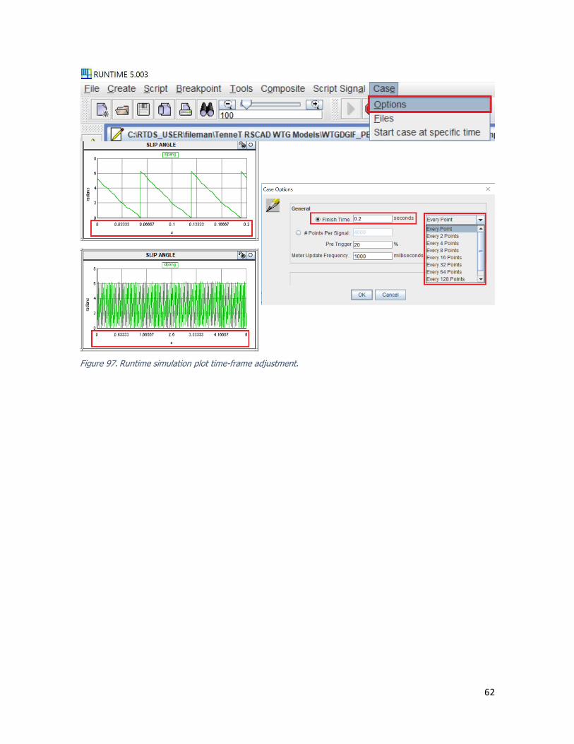
62
Figure 97. Runtime simulation plot time-frame adjustment.

63
Glossary
AC- Alternate Current. A type of electrical current in which the current repeatedly changes direction.
ABC- Transformation that represents a method of alternating current electric power generation,
transmission, and distribution. It is a type of polyphase system and is the most common
method used by electrical grids worldwide to transfer power. It is also used to power large
motors and other heavy loads.
DC- Direct Current. A type of electrical current which flows only in one direction.
DFIG- Doubly-Fed Induction Generator. It has the added benefit variable frequency ac excitation
the rotor circuit. This excitation is supplied through slip rings by a current regulated, voltage-
source converter (VSC), which allows for near instantaneous control of the rotor current
magnitude and phase. The rotor-side converter is connected in a back-to-back fashion by
using a grid side converter allowing for direct power exchange with the grid.
dq- Direct-quadrature-zero transformation. Consists of a tensor that rotates the reference frame of
a three-element vector or a three-by-three element matrix in an effort to simplify analysis.
Concept often used in the context of electrical engineering with three-phase circuits.
ECS- European Credit Transfer and Accumulation System. standard means for comparing the
"volume of learning based on the defined learning outcomes and their associated workload"
for higher education across the European Union and other collaborating European countries.
EEMCS- Faculty of Electrical Engineering, Mathematics and Computer Science.
Edc- Voltage in DC of the capacitor enclosed inside the DC power-electronics VSC converter.
EMT- Electromagnetic transients.
EMTDC- Electromagnetic transients including DC.
EWI- Elektrotechniek, Wiskunde en Informatica. Dutch translation of EEMCS.
GE- General Electric. American multinational conglomerate corporation.
GSC-Grid-Side Converter.
GTO- Gate-Turn-Off thyristor. Type of thyristor that has fully controllable switches, which can be
turned on and off by their third lead, the gate lead.
HVDC- High-Voltage Direct Current.
IEC- International Electrotechnical Commission.
IEEE- Institute of Electrical and Electronics Engineers.
IEPG- Intelligent Electrical Power Grids.
IGBT- Insulated-Gate Bipolar Transistor. It is a three-terminal power semiconductor device primarily
used as an electronic switch which, as it was developed, came to combine high efficiency and
fast switching.
INDM- Induction Machine Model.
kA- Base unit of electric current in the International System of Units (SI), with ‘kilo’ prefix.

64
kV- Base unit of electric potential, or voltage, in the International System of Units (SI), with ‘kilo’
prefix.
MIGRATE- Massive InteGRATion of power Electronic devices.
Mint condition- Is an expression used to denote the quality of a pre-owned good as displaying
virtually no imperfections and being in pristine condition relative to its original
production state. In this case, the phrase is referred to the condition that was
delivered the DFIG_PE_Tennet_V14 PSCAD model case by TenneT to the
student who developed the RSCAD wind power system module.
MVA- Mega-Volt-Ampere. Unit that quantifies complex-apparent power, with ‘Mega’ prefix.
MW- Mega-Watt. Unit that quantifies active power, with ‘Mega’ prefix.
NOT- Logic gate which implements logical negation.
PCC- Point of Common-Coupling.
PD- Partial delay.
PE- Power electronics. It is the application of solid-state electronics to the control and conversion of
electric power.
PI- Proportional-Integral controller. It is a control loop feedback mechanism widely used in industrial
control systems and a variety of other applications requiring continuously modulated control.
PLL- Phase-Locked Loop. Control system that generates an output signal whose phase is related to
the phase of an input signal.
PSCAD- Power System Computer Aided Design.
PWM- Pulse-Width Modulation. It is a modulation technique used to encode a message into a pulsing
signal. It allows the control of power supply to electrical devices, especially to inertial loads
such as motors and generators.
RLC- Impedance containing a Resistor (R), an Inductor (L) and a Capacitor (C).
RMS- Root-Mean Square. It is equal to the value of the direct current that would produce the same
average power dissipation in a resistive load.
RSC-Rotor-Side Converter.
RSCAD- Real System Computer Aided Design. Softer tool of RTDS System.
RT- Real time.
RTDS- Real-Time Digital System.
SB- Synchroniser Block.
SC- Short-Circuit. Electrical circuit that allows a current to unwittingly travel along a path with no or
a very low electrical impedance.
Type-3 WTG- Another definition to refer a Doubly Fed Induction Generator (DFIG) or Doubly Fed
Asynchronous Generator (DFAG). It is an extension of the Type 2 wind turbine.

65
TSO- Transmission System Operator. Entity involved in electric power transmission or transmission
of natural gas.
UQ- Voltage-reactive power relationship control. Method to regulate grid voltage by regulating the
wind park reactive power through the control of the turbine.
VSC- Voltage-Source Converter. Power-electronics converters whose polarity on DC voltage is usually
fixed, being smoothed by a large capacitance, which can be considered as a constant value.
WP- Wind park.
WTG- Wind Turbine Generator. Device that converts the wind's kinetic energy into electrical energy.
66
References
[1] A. Menze. MIGRATE-Massive InteGRATion of power Electronic devices. TenneT TSO GmbH.
Brussels, April 6th, 2017.
[2] Fletcher, John; Yang, Jin. Introduction to Doubly-Fed Induction Generator for Wind Power
Applications (PDF). University of Strathclyde, Glasgow.
[3] G. Venayagamoorthy. Comparison of Power System Simulations Studies on Different
Platforms – RSCAD, PSCAD/EMTDC, and Simulink SimPowerSystems. Real-Time Power and
Intelligent Systems Laboratory. University of Missouri-Rolla.
[4] IEC. IEC standard 61400-27-1, Wind turbines – Part 27-1: Electrical simulation models - Wind
turbines. Edition 1, 2015.
[5] J. C. Garcia, K. Mudunkotuwa, C. Shumski. Manitoba HVDC Research Centre. DRAFT. Migrate
project, Type-3 and Type-4 EMT model documentation.
[6] J. C. Garcia, K. Mudunkotuwa, C. Shumski. Manitoba HVDC Research Centre. DRAFT. Migrate
project, Type-3 EMT model-Release note.
[7] RTDS Technologies Inc. PSCAD to RSCAD conversion tool. USERS' GUIDE DRAFT VERSION
1.
[8] RTDS Technologies Inc. INDUCTION MACHINE MODELS (INDM).
[9] RTDS Technologies Inc. SMALL-TIME STEP VSC MODELLING.
[10] RTDS Technologies Inc. Manual Set. RSCAD TUTORIAL MANUAL.
[11] S. MÜLLER; S. et. al. (2002). Doubly Fed Induction Generator Systems for Wind
Turbines (PDF). IEEE Industry Applications Magazine. IEEE.
[12] J. L. Kirtley. Electric Power Principles. Sources, conversion, distribution and use.
Massachusetts Institute of Technology. USA. Wiley and Sons Ltd. 2010.
[13] G. Abad, J.Lopez. Doubly Fed Induction Machine. Modelling and Control for Wind Energy
Generation. Wiley and Sons. 2011.
[14] D. Xiang, L. Ran, P. J. Tavner, S. Yang. Control of a Doubly Fed Induction Generator in a
Wind Turbine During Grid Fault Ride-Through. IEEE transactions on energy conversion, vol.
21. NO. 3. September 2006.
[15] Manitoba HVDC Research Centre