Embed Size (px)
Citation preview

Department of Transportation Research and Special Programs Administration
Office of Pipeline Safety
SCHNEIDER
ENVIRONMENTAL
CONSULTING, LLC
TTO Number 14
Integrity Management Program Delivery Order DTRS56-02-D-70036
Derivation of Potential Impact Radius Formulae
for Vapor Cloud Dispersion Subject to 49 CFR 192
FINAL REPORT
Submitted by: Michael Baker Jr., Inc.
January 2005

Michael Baker Jr., Inc. OPS TTO14 – Derivation of Potential Impact Radius Formulae for Vapor Cloud Dispersion
This page intentionally left blank

Michael Baker Jr., Inc. OPS TTO14 – Derivation of Potential Impact Radius Formulae for Vapor Cloud Dispersion
Page i OPS TTO14 Final Report
2/1/2005
TTO Number 14
Derivation of Potential Impact Radius Formulae for Vapor Cloud Dispersion
Table of Contents
EXECUTIVE SUMMARY .........................................................................................................................................1 1 INTRODUCTION ................................................................................................................................................3 2 BACKGROUND...................................................................................................................................................5 3 IDENTIFY HAZARDOUS AND/OR TOXIC GASES SUBJECT TO 49 CFR 192, SUBPART O...............7
3.1 SCOPE STATEMENT.......................................................................................................................................7 3.2 GASES ROUTINELY TRANSPORTED BY PIPELINE ...........................................................................................7 3.3 HAZARDOUS AND/OR TOXIC GASES..............................................................................................................9
4 MODELING SOFTWARE EVALUATION....................................................................................................13 4.1 SCOPE STATEMENT.....................................................................................................................................13 4.2 OVERVIEW..................................................................................................................................................13 4.3 FACTORS AND VARIABLES ASSOCIATED WITH A HAZARDOUS AND/OR TOXIC GAS RELEASE.....................14 4.4 COMMERCIALLY AVAILABLE AIR DISPERSION MODELS FOR HAZARDOUS/AIR TOXIC GASES ...................15
5 DEVELOPMENT OF SIMPLIFIED PIR FORMULAE – TOXIC VAPOR CLOUD.................................19 5.1 OVERVIEW..................................................................................................................................................19 5.2 DEVELOPMENT OF BEST-FIT RELATIONSHIPS FROM EPA RMP TABLES.....................................................20 5.3 RELEASE RATE ...........................................................................................................................................24 5.4 PIR FORMULAE DERIVATION .....................................................................................................................25
5.4.1 Anhydrous Ammonia Calculations..................................................................................................26 5.4.2 Carbon Monoxide Calculations ......................................................................................................26 5.4.3 Chlorine Calculations .....................................................................................................................28 5.4.4 Hydrogen Sulfide Calculations .......................................................................................................29
5.5 FORMULAE LIMITATIONS............................................................................................................................29 5.5.1 Toxic Gas Release Example ............................................................................................................30
6 DEVELOPMENT OF SIMPLIFIED PIR FORMULAE – FLAMMABLE VAPOR CLOUD ...................31 6.1 OVERVIEW..................................................................................................................................................31 6.2 PIR FORMULAE DERIVATION .....................................................................................................................31
6.2.1 Acetylene Calculations....................................................................................................................32 6.2.2 Anhydrous Ammonia Calculations..................................................................................................32 6.2.3 Carbon Monoxide Calculations ......................................................................................................33 6.2.4 Ethylene Calculations .....................................................................................................................34 6.2.5 Hydrogen Sulfide Calculations .......................................................................................................35 6.2.6 Methane Calculations .....................................................................................................................35 6.2.7 Rich Gas Calculations.....................................................................................................................36
6.3 METHODOLOGY FOR FLAMMABLE GAS MIXTURES ....................................................................................36 6.3.1 Example of Mixed Gas Calculations ...............................................................................................37
6.4 FORMULAE LIMITATIONS............................................................................................................................38

Michael Baker Jr., Inc. OPS TTO14 – Derivation of Potential Impact Radius Formulae for Vapor Cloud Dispersion
Page ii OPS TTO14 Final Report
2/1/2005
7 FORMULAE VALIDATION............................................................................................................................39 7.1 ACETYLENE................................................................................................................................................39 7.2 ANHYDROUS AMMONIA .............................................................................................................................40 7.3 CARBON MONOXIDE...................................................................................................................................42 7.4 CHLORINE...................................................................................................................................................44 7.5 ETHYLENE ..................................................................................................................................................46 7.6 HYDROGEN SULFIDE...................................................................................................................................47 7.7 METHANE...................................................................................................................................................49
8 CONCLUSIONS.................................................................................................................................................51 9 REFERENCES ...................................................................................................................................................53 APPENDIX A INFORMATION FROM THE EPA TTN SCRAM WEBSITE.....................................................1 APPENDIX B INFORMATION FROM THE COMBOSE AIR DISPERSION MODELING SOFTWARE
WEBSITE..........................................................................................................................................11 APPENDIX C OTHER WEBSITES........................................................................................................................19
List of Figures FIGURE 5.1 COMPARISON OF BEST-FIT EQUATION TO EPA RMP TABULAR VALUES FOR CHLORINE...................21 FIGURE 5.2 COMPARISON OF BEST-FIT EQUATIONS FOR RURAL CONDITIONS ......................................................22 FIGURE 5.3 COMPARISON OF BEST-FIT EQUATIONS FOR URBAN CONDITIONS......................................................23 FIGURE 7.1 ACETYLENE – OVERPRESSURE ...........................................................................................................40 FIGURE 7.2 ANHYDROUS AMMONIA – RURAL CONDITIONS..................................................................................41 FIGURE 7.3 ANHYDROUS AMMONIA – URBAN CONDITIONS .................................................................................42 FIGURE 7.4 CARBON MONOXIDE – RURAL CONDITIONS.......................................................................................43 FIGURE 7.5 CARBON MONOXIDE – URBAN CONDITIONS ......................................................................................44 FIGURE 7.6 CHLORINE – RURAL CONDITIONS.......................................................................................................45 FIGURE 7.7 CHLORINE – URBAN CONDITIONS ......................................................................................................46 FIGURE 7.8 ETHYLENE – OVERPRESSURE .............................................................................................................47 FIGURE 7.9 HYDROGEN SULFIDE – RURAL CONDITIONS.......................................................................................48 FIGURE 7.10 HYDROGEN SULFIDE – URBAN CONDITIONS ......................................................................................49 FIGURE 7.11 METHANE – OVERPRESSURE ..............................................................................................................50

Michael Baker Jr., Inc. OPS TTO14 – Derivation of Potential Impact Radius Formulae for Vapor Cloud Dispersion
Page iii OPS TTO14 Final Report
2/1/2005
List of Tables TABLE 3.1 GASES TRANSPORTED BY PIPELINES (FROM THE NPMS)..........................................................................7 TABLE 3.2 GASES TRANSPORTED BY PIPELINE (THE PIPELINE GROUP) .....................................................................8 TABLE 3.3 GASES COVERED BY 49 CR 195 IDENTIFIED IN THE YEARLY ACCIDENT SUMMARIES 1990–2004 (OFFICE
OF PIPELINE SAFETY) ................................................................................................................................8 TABLE 3.4 GASES TRANSPORTED BY PIPELINE ........................................................................................................10 TABLE 3.5 RICH NATURAL GAS COMPOSITION CONSIDERED...................................................................................10 TABLE 3.6 GAS PHYSICAL PROPERTIES....................................................................................................................11 TABLE 4.1 AIR DISPERSION SOFTWARE FOR LIGHTER THAN AIR GAS RELEASES FROM PIPELINES..........................15 TABLE 4.2 AIR DISPERSION SOFTWARE FOR HEAVIER THAN AIR GAS RELEASES FROM PIPELINES .........................16 TABLE 4.3 MATRIX OF AVAILABLE INPUT PARAMETERS AIR DISPERSION SOFTWARE FOR LIGHTER-THAN-AIR GAS
RELEASES FROM PIPELINES.....................................................................................................................17 TABLE 4.4 MATRIX OF AVAILABLE INPUT PARAMETERS FOR AIR DISPERSION SOFTWARE FOR HEAVIER-THAN-AIR
GAS RELEASES FROM PIPELINES .............................................................................................................17 TABLE 5.1 SUMMARY OF BEST-FIT EQUATIONS.......................................................................................................20 TABLE 5.2 FACTORS FOR ANHYDROUS AMMONIA ...................................................................................................26 TABLE 5.3 FACTORS FOR CARBON MONOXIDE ........................................................................................................27 TABLE 5.4 FACTORS FOR CHLORINE ........................................................................................................................28 TABLE 5.5 FACTORS FOR HYDROGEN SULFIDE ........................................................................................................29 TABLE 6.1 FACTORS FOR ACETYLENE .....................................................................................................................32 TABLE 6.2 FACTORS FOR ANHYDROUS AMMONIA ...................................................................................................33 TABLE 6.3 FACTORS FOR CARBON MONOXIDE ........................................................................................................33 TABLE 6.4 FACTORS FOR ETHYLENE........................................................................................................................34 TABLE 6.5 FACTORS FOR HYDROGEN SULFIDE ........................................................................................................35 TABLE 6.6 FACTORS FOR METHANE.........................................................................................................................35 TABLE 6.7 FACTORS FOR RICH GAS.........................................................................................................................36 TABLE 6.8 MIXED GAS PROPERTIES AND COMPOSITION..........................................................................................37 TABLE 7.1 COMPARISON OF DISTANCE CALCULATED ACETYLENE (OVERPRESSURE) .............................................39 TABLE 7.2 COMPARISON OF DISTANCE CALCULATED ANHYDROUS AMMONIA (RURAL CONDITIONS)....................40 TABLE 7.3 COMPARISON OF DISTANCE CALCULATED ANHYDROUS AMMONIA (URBAN CONDITIONS) ...................41 TABLE 7.4 COMPARISON OF DISTANCE CALCULATED CARBON MONOXIDE (RURAL CONDITIONS) .........................42 TABLE 7.5 COMPARISON OF DISTANCE CALCULATED CARBON MONOXIDE (URBAN CONDITIONS).........................43 TABLE 7.6 COMPARISON OF DISTANCE CALCULATED CHLORINE (RURAL CONDITIONS) .........................................44 TABLE 7.7 COMPARISON OF DISTANCE CALCULATED CHLORINE (URBAN CONDITIONS).........................................45 TABLE 7.8 COMPARISON OF DISTANCE CALCULATED ETHYLENE (OVERPRESSURE)................................................46 TABLE 7.9 COMPARISON OF DISTANCE CALCULATED HYDROGEN SULFIDE (RURAL CONDITIONS) .........................47 TABLE 7.10 COMPARISON OF DISTANCE CALCULATED HYDROGEN SULFIDE (URBAN CONDITIONS) ....................48 TABLE 7.11 COMPARISON OF DISTANCE CALCULATED METHANE (OVERPRESSURE) ............................................49 TABLE 8.1 SUMMARY OF PIR FORMULAE................................................................................................................51

Michael Baker Jr., Inc. OPS TTO14 – Derivation of Potential Impact Radius Formulae for Vapor Cloud Dispersion
Page iv OPS TTO14 Final Report
2/1/2005
This page intentionally left blank

Michael Baker Jr., Inc. OPS TTO14 – Derivation of Potential Impact Radius Formulae for Vapor Cloud Dispersion
Page 1 OPS TTO14 Final Report
02/01/05
Executive Summary This report was prepared in accordance with the Statement of Work and proposal submitted in response to RFP for Technical Task Order Number 14 (TTO 14) entitled “Derivation of Potential Impact Radius Formulae for Hazardous and/or Toxic Gases Without Ignition”, dated July 2004. Subsequent to the development of the initial statement of work, the scope was expanded to include delayed vapor cloud ignition.
A key element of the Gas Integrity Management Rule (49 CFR 192, Subpart O) is the calculation of the potential impact radius (PIR) of a circle within which the potential failure of a pipeline could have significant impact on people or property.
The original derivation of the PIR formula referenced in 49 CFR 192 is contained in the Gas Research Institute (GRI) report by C-FER Technologies (C-FER), “A Model for Sizing High Consequence Areas Associated with Natural Gas Pipelines” (Stephens 2000). This formula was derived solely on the premise that a thermal radiation from a jet/trench fire is the dominant hazard related to pipe rupture and subsequent ignition. (The Michael Baker Jr. Inc. report for TTO13, entitled Potential Impact Radius Formulae for Flammable Gases Other Than Natural Gas Subject to 49 CFR 192, Subpart O, discusses and develops an extension to the above formula, generalizing the formula for application to jet/trench fires to flammable gases transported by pipelines under the OPS jurisdiction).
However, the threat from a release of a gas product is not limited to ignition of the jet in the ditch and the subsequent thermal radiation. There are at least two other threats posed by rupture of a gas pipeline:
1) A vapor cloud flash fire, when ignition does not occur in the trench, allowing the formation of a vapor cloud that will drift downwind until it encounters an ignition source. This threat is particularly applicable to flammable gases with specific gravities greater than or near that of air, such as ethylene. Note that the size (or downwind extent) of the flammable cloud could exceed the jet fire thermal radiation hazard and, in any case, potentially extends the threat zone outside the Right-of-Way (ROW) limits.
2) Formation of a toxic gas cloud, which again may drift downwind, potentially extending the threat zone outside ROW limits. Several factors, including the amount and rate of release, the toxicity concentration level, natural and forced dispersion of the gas, and meteorological factors should be considered when examining threat possibilities.
These threats are the subject of this report. Although this report is limited to transported gas products covered by 49 CFR 192, it is noted that some transported liquids will, upon release, flash into a gas that may form a toxic/flammable vapor cloud. Although such products are outside the scope of the study, such a product release scenario could also be examined using the procedures developed in this report.
A general introduction is contained in Section 1, while Section 2 presents more detailed information regarding the basic differences between a jet fire release and the behavior of a toxic gas upon release.

Michael Baker Jr., Inc. OPS TTO14 – Derivation of Potential Impact Radius Formulae for Vapor Cloud Dispersion
Page 2 OPS TTO14 Final Report
02/01/05
Section 3 documents the process utilized in identifying the various products that are known or reasonably assumed to be currently transported by pipeline in the U.S. Four products were chosen for development of a simplified PIR formula: anhydrous ammonia (even though it is normally transported as a liquid under pressure), carbon monoxide, chlorine and hydrogen sulfide.
Section 4 presents a summary of computer software available for modeling the dispersion of gases that are most applicable to pipeline type releases. The majority of these software products consider more generic releases and therefore require additional calculations to convert pipeline related data in the form accepted by the program. Additional information on modeling software is presented in Appendices A, B and C.
Section 5 describes the process used to develop simplified PIR formulae for each of the hazardous/toxic products identified in Section 3. The basis for the formulae development was the US Environmental Protection Agency’s (EPA) “Risk Management Program Guidance for Offsite Consequence Analysis”, drawing on the GRI report mentioned above.
Section 6 describes the process used to develop simplified PIR formulae for each of the flammable products identified in Section 3 using a 1 psi overpressure as the threshold criteria. The basis for the formulae development was the U.S. Environmental Protection Agency’s (EPA) “Risk Management Program Guidance for Offsite Consequence Analysis”, drawing on the GRI report mentioned above.
Section 7 describes the efforts conducted to validate the formulae by comparing results from several examples to results obtained using the EPA document. Section 8 presents the general conclusions of the report, with Section 9 presenting a list of reference documents used in the report.

Michael Baker Jr., Inc. OPS TTO14 – Derivation of Potential Impact Radius Formulae for Vapor Cloud Dispersion
Page 3 OPS TTO14 Final Report
02/01/05
1 Introduction This report was prepared in accordance with the Statement of Work and proposal submitted in response to RFP for Technical Task Order Number 14 (TTO 14) entitled “Derivation of Potential Impact Radius Formulae for Hazardous and/or Toxic Gases Without Ignition”, dated July 2004. Subsequent to the development of the initial statement of work, the scope was expanded to include delayed vapor cloud ignition.
A key element of the Gas Integrity Management Rule (49 CFR 192, Subpart O) is the calculation of the potential impact radius (PIR) of a circle within which the potential failure of a pipeline could have significant impact on people or property. Subpart O provides a specific formula for the calculation of this PIR that is to be used for natural gas:
269.0 dpr ⋅⋅=
where:
r = the PIR in feet,
p = the pipeline maximum operating pressure in pounds per square inch, and
d = the nominal pipeline diameter in inches.
However, the above formula was derived solely on the premise that a thermal radiation from a jet/trench fire is the dominant hazard related to pipe rupture and subsequent ignition. (The Michael Baker Jr. Inc. report for TTO13, entitled Potential Impact Radius Formulae for Flammable Gases Other Than Natural Gas Subject to 49 CFR 192, Subpart O, discusses and develops an extension to the above formula, generalizing the formula for application to jet/trench fires to flammable gases transported by pipelines under the OPS jurisdiction).
The threat from a release of a gas product is not limited to ignition of the jet in the ditch and the subsequent thermal radiation. There are at least two other threats posed by rupture of a gas pipeline:
1) A vapor cloud flash fire, when ignition does not occur in the trench, allowing the formation of a vapor cloud that will drift downwind until it encounters an ignition source. This threat is particularly applicable to flammable gases with specific gravities greater than or near that of air, such as ethylene. Note that the size (or downwind extent) of the flammable cloud could exceed the jet fire thermal radiation hazard.
2) Formation of a toxic gas cloud, which again may drift downwind, potentially extending the threat zone outside ROW limits. Several factors, including the amount and rate of release, the toxicity concentration level, natural and forced dispersion of the gas, and meteorological factors should be considered when examining threat possibilities.
The threats of a toxic gas cloud and a vapor cloud flash fire are the subject of this report. Although this report is limited to transported gas products covered by 49 CFR 192, it is noted that some transported liquids will, upon release, flash into a gas that may form a toxic/flammable vapor cloud. Although such products are outside the scope of the study, such a product release scenario could also be examined using the procedures developed in this report.

Michael Baker Jr., Inc. OPS TTO14 – Derivation of Potential Impact Radius Formulae for Vapor Cloud Dispersion
Page 4 OPS TTO14 Final Report
02/01/05
This page intentionally left blank
Michael Baker Jr., Inc. OPS TTO14 – Derivation of Potential Impact Radius Formulae for Vapor Cloud Dispersion
Page 5 OPS TTO14 Final Report
02/01/05
2 Background The failure of a gas pipeline can lead to various outcomes, some of which can pose a significant threat to people and property in the immediate vicinity of the failure location. For a given pipeline, the type of hazard that develops (i.e., flammable vs. toxic), and the damage or injury potential associated with the hazard, will depend on the type of gas, the mode of line failure (i.e., leak vs. rupture), the nature of gas discharge (i.e., vertical vs. inclined jet, obstructed vs. unobstructed jet), the meteorological conditions prevalent during the release (i.e., wind speed and direction) and, in the case of flammable gas, the time to ignition (i.e., immediate vs. delayed).
Toxic gases, as well as some flammable gases, will, upon release, form a vapor cloud with the highest concentration near the source. The vapor will disperse with the near atmospheric volume until, at some distance away from the source, the concentration will be at or below lethal/explosive levels. An analogy to the “potential impact radius” for the jet/trench fire, defined as the areal extent for which the potential failure of a pipeline could have significant effect on people, is that extent wherein the concentration of the toxic gas is at or above lethal levels. In the case of a flammable gas, the potential impact radius can be defined as the distance to an overpressure of 1 psi.
In this discussion, “areal extent” is used in lieu of “radius”, which is used in the explanation of jet/trench fire. Rarely will the area of significant impact for vapor clouds be defined as a circle, as is implied for the jet/trench fire and substantiated by the relatively straightforward thermal radiation theoretical formulae associated with this hazard. Instead, the extent of a vapor cloud from a point release is described using dispersion formulae which are governed by meteorological conditions, mainly wind direction and velocity. Thus, the areal extent of a vapor cloud is most commonly defined as a “plume” emanating from the source and increasing in a rough wedge-like pattern with distance from the source.
However, in the development of simplified formulae for sizing the impact of a release discussed in Sections 5 and 6, the form is given using a PIR to provide a generalized approach. Given sufficient data regarding a site-specific location, the case might be argued to modify the shape of the final impact zone from a circle to a wedge or plume, though such a modification would reasonably require a more sophisticated analysis than that used in this report.

Michael Baker Jr., Inc. OPS TTO14 – Derivation of Potential Impact Radius Formulae for Vapor Cloud Dispersion
Page 6 OPS TTO14 Final Report
02/01/05
This page intentionally left blank

Michael Baker Jr., Inc. OPS TTO14 – Derivation of Potential Impact Radius Formulae for Vapor Cloud Dispersion
Page 7 OPS TTO14 Final Report
02/01/05
3 Identify Hazardous and/or Toxic Gases Subject to 49 CFR 192, Subpart O 3.1 Scope Statement
“Identify hazardous and/or toxic gases that are routinely transported by the pipeline industry and which would be subject to the requirements of 49 CFR 192, Subpart O.”
3.2 Gases Routinely Transported by Pipeline
A search of data housed within the National Pipeline Mapping System (NPMS) generated a short list of gases that are transported by pipeline (presented in Table 3.1). However, the broad category, “Other Gas”, could cover numerous commodities, that could be potentially hazardous/toxic and/or flammable.
A range of nominal pipe sizes (NPS) associated with each gas identified in the NPMS and the governing regulation are also presented. Operators are not required to provide the NPS for inclusion into the NPMS, and the NPS default value is zero. Thus, in most cases only the maximum NPS reported is shown.
Table 3.1 Gases Transported by Pipelines (from the NPMS)
Commodity Governing Pipeline Regulation NPS
Anhydrous Ammonia 49 CFR 195 ≤10 Carbon Dioxide 49 CFR 195 ≤30 Hydrogen Gas 49 CFR 192 2 to 20 Natural Gas 49 CFR 192 Not available1 Other Gas 49 CFR 192 6 to 12
1 The largest gas pipeline NPS listed by the American Gas Association (AGA) is 42.
Further searches yielded a list of gases transported by pipeline based on material safety data sheets (MSDS) information presented by The Pipeline Group. These gases are presented in Table 3.2.

Michael Baker Jr., Inc. OPS TTO14 – Derivation of Potential Impact Radius Formulae for Vapor Cloud Dispersion
Page 8 OPS TTO14 Final Report
02/01/05
Table 3.2 Gases Transported by Pipeline (The Pipeline Group)
Commodity Governing Pipeline Regulation
Acetylene Anhydrous Ammonia 49 CFR 1951 Butadiene Butane 49 CFR 1951 Butene Carbon Dioxide 49 CFR 1951 Carbon Monoxide 49 CFR 192 Ethane 49 CFR 1951 Ethylene 49 CFR 1951 Hydrogen 49 CFR 192 Hydrogen Sulfide 49 CFR 192 Methane 49 CFR 192 Propane 49 CFR 1951 Propylene 49 CFR 1951
1 49 CR 195 is shown as the governing regulation for these gases since they are listed in the Liquid Accident Yearly Summaries on the OPS website.
Some commodities that are liquefied under normal operating pressures for pipelines will quickly volatilize into a vapor when released. In order to identify any such commodities for which a significant threat resulting from accidental release would be the formation of a vapor cloud, an evaluation of the Liquid Accidental Yearly Summaries from 1990 through 2004 from the OPS website was conducted. These summaries identify the number and amounts of liquefied gases released over the last 15 years. Table 3.3 presents the compilation of liquefied gases identified from the OPS yearly accident summaries.
Table 3.3 Gases Covered by 49 CR 195 Identified in the Yearly Accident Summaries 1990–2004
(Office of Pipeline Safety) Commodity
Anhydrous Ammonia Butane Carbon Dioxide Ethane Ethylene LPG Natural Gas Liquid Propane Propylene
While no searches identified chlorine gas as being transported by pipeline, OPS indicated that there are chlorine pipelines currently being operated under the jurisdiction of 49 CFR 192.

Michael Baker Jr., Inc. OPS TTO14 – Derivation of Potential Impact Radius Formulae for Vapor Cloud Dispersion
Page 9 OPS TTO14 Final Report
02/01/05
3.3 Hazardous and/or Toxic Gases
Poisonous gases are defined by the U.S. Department of Transportation under 49 CFR 173 Subpart D as:
...a material which is a gas at 20 °C (68 °F) or less and a pressure of 101.3 kPa (14.7 psia) (a material which has a boiling point of 20 °C (68 °F) or less at 101.3 kPa (14.7 psia)) and which—
(1) Is known to be so toxic to humans as to pose a hazard to health during transportation, or
(2) In the absence of adequate data on human toxicity, is presumed to be toxic to humans because when tested on laboratory animals it has an LC50 value of not more than 5000 mL/m 3 (see §173.116(a) of this subpart for assignment of Hazard Zones A, B, C or D). LC50 values for mixtures may be determined using the formula in §173.133(b)(1)(i) or CGA Pamphlet P–20 (IBR, see §171.7 of this subchapter).
Flammable gases are defined by the U.S. Department of Transportation under 49 CFR 115 Subpart D as:
...any material which is a gas at 20°C (68°F) or less and 101.3 kPa (14.7 psi) of pressure (a material which has a boiling point of 20oC (68oF) or less at 101.3 kPa (14.7 psi)) which-
1. Is ignitable at 101.3 kPa (14.7 psi) when in a mixture of 13 percent or less by volume with air; or
2. Has a flammable range at 101.3 kPa (14.7 psi) with air of at least 12 percent regardless of the lower limit.
Except for aerosols, the limits specified in paragraphs (a)(1) and (a)(2) of this section shall be determined at 101.3 kPa (14.7 psi) of pressure and a temperature of 20oC (68oF) in accordance with ASTM E681-85, Standard Test Method for Concentration Limits of Flammability of Chemicals or other equivalent method approved by the Associate Administrator for Hazardous Materials Safety.
Combining the information presented in Section 3.2 results in the list of gases presented in Table 3.4. This list was compared against lists of hazardous/toxic substances given in the OSHA (29 CFR 1910) and the EPA (40 CFR 68) regulations. Gases listed in these regulations are marked in the corresponding column within the table. Gases noted as flammable were identified as such by the National Fire Protection Association with the exception of anhydrous ammonia.

Michael Baker Jr., Inc. OPS TTO14 – Derivation of Potential Impact Radius Formulae for Vapor Cloud Dispersion
Page 10 OPS TTO14 Final Report
02/01/05
Table 3.4 Gases Transported by Pipeline Hazardous/Toxic
Commodity Formula Governing Pipeline Regulation Flammable
29 CFR 1910 40 CFR 68 Acetylene C2H2 Y N N Anhydrous Ammonia NH4 49 CFR 195 Y Y Y Butadiene C4H6 Y N N Butane C4H10 49 CFR 195 Y N N Butene C4H8 Y N N Carbon Dioxide CO2 49 CFR 195 N N N Carbon Monoxide1 CO 49 CFR 192 Y N N Chlorine Cl2 49 CFR 192 N Y Y Ethane C2H6 49 CFR 195 Y N N Ethylene C2H4 49 CFR 195 Y N N Hydrogen H2 49 CFR 192 Y N N Hydrogen Sulfide H2S 49 CFR 192 Y Y Y Methane CH4 49 CFR 192 Y N N Propane/LPG2 C3H8 49 CFR 195 Y N N Propylene C3H6 49 CFR 195 Y N N
1 Listed as toxic in the California Fire Code, by the National Fire Protection Association, and other references. 2 LPG and propane were combined into one category for simplicity.
The commodities chosen for evaluation were those considered hazardous/toxic by both EPA and OSHA (anhydrous ammonia, chlorine, and hydrogen sulfide), carbon monoxide based on its classification as a toxic chemical by California Fire Code, acetylene, ethylene and methane. “Rich” natural gas (as opposed to pure methane or “lean” gas) was also chosen to provide additional definition for natural gas transportation (see Table 3.5 for gas composition). While hydrogen is highly flammable, due to its low molecular weight, it is highly unlikely that a flammable vapor cloud could form following a pipeline rupture. In addition, while an analysis was completed for acetylene, it is unlikely that acetylene is actually transported via pipelines subject to 49 CFR 192 since at a pressure around 30 psi, acetylene can polymerize explosively even without an admixture of air. References to acetylene pipelines found during research for this study indicate that existing systems operate at a pressure of 15 psi or less and are largely limited to industrial use such as shipyards for oxy-acetylene cutting and welding. The physical properties of the gases considered are presented in Table 3.6.
Table 3.5 Rich Natural Gas Composition Considered
Compound Composition (%)
Methane 80.0 Ethane 15.0 Propane 3.0 Butane 0.5 Nitrogen 0.5 Carbon Dioxide 0.5 Other 0.5

Michael Baker Jr., Inc. OPS TTO14 – Derivation of Potential Impact Radius Formulae for Vapor Cloud Dispersion
Page 11 OPS TTO14 Final Report
02/01/05
Table 3.6 Gas Physical Properties
Commodity Acetylene Anhydrous Ammonia
Carbon Monoxide Chlorine Ethylene Hydrogen
Sulfide Methane Rich Gas
Formula C2H2 NH3 CO Cl2 C2H4 H2S CH4 Varies Molecular Weight (lbm/lb-mole) 26.04 17.03 28.01 70.91 28.05 34.08 16.04 19.5
Boiling Point at 1 atm (°F) -118.9 -28.2 -312.8 -29.4 -154.7 -76.4 -258.8 cp 0.382 0.523 0.247 0.114 0.362 0.239 0.534 Specific Heat
(Btu/lbm °F) cv 0.303 0.399 0.176 0.084 0.291 0.181 0.409 Cp 9.95 8.91 6.92 8.08 10.15 8.14 8.57 Heat Capacity
(Btu/mole °F) Cv 7.89 6.80 4.93 5.96 8.16 6.17 6.56 Heat of Vaporization at bp
(Btu/lbm) 344.75 589 92.4 123.7 207.6 235.4 219.3
Specific Gravity 0.91 0.60 0.97 2.49 0.97 1.19 0.55 0.67 Density at STD (lb/ft3) 0.069 0.045 0.073 0.189 0.073 0.09 0.042
Liquid Density at bp (lb/ft3) 42.58 49.23 97.54 35.45 57.12 26.38 Heat of Combustion (BTU/lbm) 20,769 7,985 4,347 NA 20,275 6,537 21,495 20,588
Specific Heat Ratio 1.26 1.31 1.40 1.36 1.24 1.32 1.31 1.29
Toxicity End Points (mg/L) NA 0.14 1.725 0.0087 NA 0.042 NA NA
LC50/1h1 (ppm) NA 4000 3760 293 NA 712 NA NA 1 LC50/1h stands for Lethal Concentration where inhalation kills 50% of the test animals in an hour.
The gases identified in Table 3.6 can be further classified into lighter-than-air, heavier-than-air or neutrally-buoyant, the distinction being when the molecular weight of the gas is less than, greater than, or approximately equal to air’s molecular weight of approximately 29. Anhydrous ammonia, methane and rich gas are lighter-than-air, chlorine and hydrogen sulfide are heavier-than-air, while acetylene and carbon monoxide are considered neutrally-buoyant. This distinction is important when evaluating potential air dispersion modeling software for predicting downwind concentrations.
Similar to rich gas, there are potentially numerous other flammable gas mixtures or “mixed” gas (e.g., land-fill gas) for which the derivation of a PIR formula may be desirable. Therefore, a methodology for calculation of an appropriate PIR for mixed gas composed of common elements is also discussed later in this report.

Michael Baker Jr., Inc. OPS TTO14 – Derivation of Potential Impact Radius Formulae for Vapor Cloud Dispersion
Page 12 OPS TTO14 Final Report
02/01/05
This page intentionally left blank

Michael Baker Jr., Inc. OPS TTO14 – Derivation of Potential Impact Radius Formulae for Vapor Cloud Dispersion
Page 13 OPS TTO14 Final Report
02/01/05
4 Modeling Software Evaluation 4.1 Scope Statement
“Survey and evaluate commercially available modeling software (to include but not be limited to entries at http://www.combose.com/Science/Environment/Air_Quality/Air_Dispersion_Modeling/Software/) to determine the applicability of available analytical techniques for determining the PIR that may result from a potential release of hazardous and/or toxic gases (those identified in Subtask 01) from a gas transmission line. The analytical techniques, as a minimum, should account for the following factors and variables:
a. physical properties of the gas
b. toxicity of the released gas
c. maximum pipeline operating pressure
d. pipeline nominal diameter
e. potential rupture size (e.g., small rupture or double guillotine break)
f. potential meteorological conditions”
4.2 Overview
A survey and evaluation of applicable commercially available air dispersion modeling software for a potential release of hazardous and/or toxic gases was performed. The survey evaluated numerous governmental, organizational, and private web links. Brief descriptions for a number of air-dispersion software, actual air-dispersion models or other information related to air dispersion are presented in Appendices A, B and C of this report, including the web address cited in the scope of work. Several of these links either are no longer valid or have restricted access. Many of the models referenced are for determining impacts from mobile sources or industrial stacks and are not applicable for analysis of accidental releases from pipelines. At least two of the models are specific to the dispersion of aircraft exhaust plumes. Many of the software products are based on EPA models such as the Gaussian dispersion models, SLAB, DEGADIS, etc.
After the initial evaluation to determine applicable air dispersion modeling software for analyzing hazardous and/or toxic gas releases from pipelines was completed, an assessment of the analytical techniques for each, including a review of the available input parameters, was conducted.
The survey and evaluation concluded that the best resource to utilize for air dispersion modeling is the EPA – Technology Transfer Network (TTN) – Support Center for Regulatory Air Models (SCRAM) located at website:
http://www.epa.gov/scram001/
The “Dispersion Models” link at this website provide a plethora of current information regarding air dispersion modeling applicability and is arranged by the following topics:
• Preferred/Recommended Models,

Michael Baker Jr., Inc. OPS TTO14 – Derivation of Potential Impact Radius Formulae for Vapor Cloud Dispersion
Page 14 OPS TTO14 Final Report
02/01/05
• Screening Tools,
• Alternative Models,
• Related Programs, and
• Model Tutorials.
A list of available software is provided for each topic with links to a variety of information on each program (e.g., user’s guide, user’s guide addendum, model change bulletin, etc.).
4.3 Factors and Variables Associated with a Hazardous and/or Toxic Gas Release
The analysis of many chemical release scenarios is a function of numerous input parameters and their associated range of variability, and will depend on the particular dispersion modeling software selected. Air dispersion modeling capabilities and results vary widely from a screening level to detailed site-specific analyses. Key incident specific input parameters include:
• Molecular weight of the gas.
• Quantity released, including release duration, release rates, release velocities, and angles of release (from horizontal to vertical).
• Meteorological conditions (stability class and wind speed).
• Surface Roughness for Heavy Gas dispersion.
Molecular weight of the gas: The molecular weight of the gas to be modeled (more exactly, the specific gravity with respect to air) helps in the selection of the proper air dispersion model for predicting the distance of the toxic endpoint mainly by allowing the gas to be classified as lighter-than-air, neutrally buoyant or denser-than-air. Dense gases behave quite differently from lighter-than-air or neutrally buoyant gases when released to the atmosphere.
Quantity Released: The peak release rate from a guillotine pipeline rupture is a function of the pipeline diameter and the internal pressure. After the initial rupture, the release rate will decay rapidly as the system depressurizes. The temperature and pressure of the release will determine the size of the vapor cloud along with the angle of release (horizontal or vertical).
Meteorological Conditions: Meteorological conditions including wind speed and atmospheric stability can vary. Atmospheric stability is normally defined using standard Pasquill-Gifford stability classes, which range from very unstable (class A) to stable (class F). Screening model wind speed inputs can range from 0.5 to 20 m/s. For screening modeling purposes, one set of meteorological conditions are typically used for predicting the worst-case impacts (least dispersion): wind speed of 1.5 m/s and an atmospheric stability of class F.
Surface Roughness: Surface roughness is a function of a rural or urban setting. This parameter will only impact heavy gas or dense gas dispersion because the vapor release will stay at ground level. If the site is located in an area with few buildings or other obstructions, rural conditions are assumed. If the site is an urban location, or is in an area with many obstructions, urban conditions should be assumed.

Michael Baker Jr., Inc. OPS TTO14 – Derivation of Potential Impact Radius Formulae for Vapor Cloud Dispersion
Page 15 OPS TTO14 Final Report
02/01/05
4.4 Commercially Available Air Dispersion Models for Hazardous/Air Toxic Gases
A number of air dispersion models that are available on EPA TTN SCRAM Bulletin Board can be downloaded for free. Commercial software companies (i.e. Trinity Consultants, Beeline, etc.) have enhanced the free version from EPA and provide a more “user-friendly version” providing more “Bells and Whistles”. Through evaluation of the air dispersion modeling software presented in Appendices A, B and C, a list of software applicable to analyzing pipeline related releases are summarized in Table 4.1 and Table 4.2 for lighter than air and heavier than air gases, respectively. These software products have varying capabilities of input (e.g., calculation of release quantity, etc.) and output sophistication for modeling a hazardous/toxic pipeline release.
Table 4.1 Air Dispersion Software for Lighter Than Air Gas Releases from Pipelines
Model Description Cost RMP*Comp RMP*Comp is computerized version of the EPA RMP lookup tables that can be used to perform the off-site
consequence analysis required under the Risk Management Program rule published by the Environmental Protection Agency on July 20, 1996, which implements Section 112(r) of the Clean Air Act. Previously, EPA has referred to this tool as RMP Calculator or RMP Assistant. http://yosemite.epa.gov/oswer/ceppoweb.nsf/content/rmp-comp.htm
Free
AFTOX – (Air Force Toxics
Model)
AFTOX is a Gaussian dispersion model that will handle continuous or instantaneous liquid or gas elevated or surface releases from point or area sources. Output consists of concentration contour plots, concentration at a specified location, and maximum concentration at a given elevation and time. http://www.epa.gov/scram001/tt22.htm
Free
ALOHA – (Areal
Locations of Hazardous
Atmospheres)
ALOHA can be used to predict the rates at which neutrally buoyant or heavier-than-air chemical vapors may escape into the atmosphere from broken gas pipes, leaking tanks, and evaporating puddles. It can predict how a hazardous gas cloud might disperse in the atmosphere after an accidental release. http://www.epa.gov/ceppo/cameo/aloha.htm
Free
HGSYSTEM A collection of computer programs designed to predict the source-term and subsequent dispersion of accidental chemical releases with an emphasis on denser-than-air (dense gas) behavior. Available from NTIS, Order Number PB96-501960. http://www.ntis.gov/search/product.asp?ABBR=PB96501960&starDB=GRAHIST
$201
INPUFF INPUFF is a Gaussian puff model that simulates the atmospheric dispersion of neutrally buoyant or buoyant chemical releases. The model accounts for point sources and a release duration that is either finite or continuous. INPUFF can account for plume rise, due to buoyancy and momentum, as well as stack tip downwash. www.breeze-software.com
$2,995
ISC3 ISC3 (Industrial Source Complex Model) is a steady-state Gaussian plume model, which can be used to assess pollutant concentrations from a wide variety of sources associated with an industrial complex. This model can account for the following: settling and dry deposition of particles; downwash; point, area, line, and volume sources; plume rise as a function of downwind distance; separation of point sources; and limited terrain adjustment. ISCST operates in both long-term and short-term modes http://www.epa.gov/scram001/tt22.htm#rec
Free
PUFF-PLUME PUFF-PLUME is a Gaussian atmospheric transport chemical/radionuclide diffusion model that includes wet and dry deposition, real-time input of meteorological observations and forecasts, dose estimates from inhalation and gamma shine, and puff or plume dispersion modes. It is the primary model for emergency response use for atmospheric releases at the Savannah River Site. It is one of a suite of codes for atmospheric releases and is used primarily for first-cut results in emergency situations. (Other codes containing more detailed mathematical and physical models are available for use when short response time is not the over-riding consideration.)
TSCREEN (Toxics
Screening)
TSCREEN is a Gaussian model that implements the procedures to correctly analyze toxic emissions and their subsequent dispersion from one of many different types of possible releases for superfund sites. It contains 3 models within it, SCREEN3, PUFF, and RVD (Relief Valve Discharge). http://www.epa.gov/scram001/tt22.htm
Free

Michael Baker Jr., Inc. OPS TTO14 – Derivation of Potential Impact Radius Formulae for Vapor Cloud Dispersion
Page 16 OPS TTO14 Final Report
02/01/05
Table 4.2 Air Dispersion Software for Heavier Than Air Gas Releases from Pipelines
Model Description Cost RMP*Comp RMP*Comp is an electronic tool used to perform the off-site consequence analysis required
under the Risk Management Program rule published by the Environmental Protection Agency on July 20, 1996, which implements Section 112(r) of the Clean Air Act. Previously, EPA has referred to this tool as RMP Calculator or RMP Assistant. http://yosemite.epa.gov/oswer/ceppoweb.nsf/content/rmp-comp.htm
Free
ADAM - (Air Force
Dispersion Assessment
Model)
A modified box and Gaussian dispersion model which incorporates thermodynamics, chemistry, heat transfer, aerosol loading, and dense gas effects. Release scenarios include continuous and instantaneous, area and point, pressurized and unpressurized, and liquid/vapor/two-phased options. http://www.epa.gov/scram001/tt22.htm
Free
ALOHA – (Areal
Locations of Hazardous
Atmospheres)
Can predict the rates at which chemical vapors may escape into the atmosphere from broken gas pipes, leaking tanks, and evaporating puddles. It can predict how a hazardous gas cloud might disperse in the atmosphere after an accidental release. http://www.epa.gov/ceppo/cameo/aloha.htm
Free
DEGADIS - (Dense Gas Dispersion
Model)
Simulates the atmospheric dispersion at ground-level, area source dense gas (or aerosol) clouds released with zero momentum into the atmospheric boundary layer over flat, level terrain. The model describes the dispersion processes which accompany the ensuing gravity-driven flow and entrainment of the gas into the boundary layer. http://www.epa.gov/scram001/tt22.htm
Free
PHAST – (Process Hazard Analysis Software
Tools)
An advanced, MS Windows® based consequence modeling program that examines the progress of a potential incident from initial release through formation of a cloud or pool to final dispersion. Consequence results may be overlayed on maps, satellite photos and plant layouts. DNV Technica – http://www.acutech-consulting.com/software/phast.html
$30,000+
SLAB The SLAB model treats denser-than-air releases by solving the one-dimensional equations of momentum, conservation of mass, species, and energy, and the equation of state. SLAB handles release scenarios including ground level and elevated jets, liquid pool evaporation, and instantaneous volume sources. http://www.beeline-software.com/slab_for_windows.htm http://www.epa.gov/scram001/tt22.htm (Original DOS version)
$950 Free
As stated previously, the capabilities of the selected air dispersion models varies based upon the parameters selected. The majority of the models summarized above require the user to calculate the release quantity and rate for input into the model. Available input parameters for lighter than air and heavier than air gases for each air dispersion model are presented in Table 4.3 and Table 4.4, respectively.

Michael Baker Jr., Inc. OPS TTO14 – Derivation of Potential Impact Radius Formulae for Vapor Cloud Dispersion
Page 17 OPS TTO14 Final Report
02/01/05
Table 4.3 Matrix of Available Input Parameters Air Dispersion Software for Lighter-than-Air Gas Releases from Pipelines
Parameter Model
A B C D E F RMP*Comp X X X AFTOX X X X ALOHA X X HGSYSTEM X X INPUFF X X X ISC3 X X PUFF-PLUME X X TSCREEN X X X A – Physical properties of gas B – Toxicity of gas C – Pipeline operating pressure D – Pipeline diameter E – Size of rupture (e.g., small rupture or double guillotine break) F – Potential meteorological conditions
Table 4.4 Matrix of Available Input Parameters for Air Dispersion Software for Heavier-than-Air Gas Releases from Pipelines
Parameter Model
A B C D E F RMP*Comp X X X ADAM X X X ALOHA X X DEGADIS X X X PHAST X X X X X X SLAB X X A – Physical properties of gas B – Toxicity of gas C – Pipeline operating pressure D – Pipeline diameter E – Size of rupture (e.g., small rupture or double guillotine break) F – Potential meteorological conditions

Michael Baker Jr., Inc. OPS TTO14 – Derivation of Potential Impact Radius Formulae for Vapor Cloud Dispersion
Page 18 OPS TTO14 Final Report
02/01/05
This page intentionally left blank

Michael Baker Jr., Inc. OPS TTO14 – Derivation of Potential Impact Radius Formulae for Vapor Cloud Dispersion
Page 19 OPS TTO14 Final Report
02/01/05
5 Development of Simplified PIR Formulae – Toxic Vapor Cloud 5.1 Overview
In the absence of more sophisticated modeling software, a simplified technique for determining the PIR for hazardous/toxic gases is desired. This technique should account for, at a minimum:
• the physical properties of the gas,
• the toxicity of the gas,
• the maximum operating pressure,
• the pipeline diameter, and
• potential meteorological conditions.
The EPA publishes a document, Risk Management Program Guidance for Offsite Consequence Analysis (EPA 1999), that provides guidance on how to conduct an offsite consequence analysis for Risk Management Programs required by the Clean Air Act. The document gives two scenarios that can be used for consequence analysis: worst-case release and alternative release. The main parameter that must be determined for application of this guidance document for the worst-case scenario is the release rate. Once the release rate is calculated, the distance to the toxic endpoint, which could also be considered the radius of impact, is determined by using a series of “lookup” tables and is based on an assumed 10-minute release duration.
The basic assumptions for the worst-case scenario are:
• Wind speed is 1.5 m/s (4.9 fps),
• Meteorological stability is standard Pasquill-Gifford stability class F1,
• Ambient temperature is 25°C (77°F),
• Relative humidity is 50 percent,
• Height of release is ground level, and
• Temperature of released product is 25°C (77°F) or the boiling point of the released product.
• Surface roughness is one of two categories:
o Rural (flat or unobstructed terrain), or
o Urban (obstructed terrain)
The program RMP*Comp is essentially an electronic version of the tables in the EPA RMP document: the main difference being that the primary input parameter is quantity of product released rather than release rate. However, the quantity of product released is simply the release rate
1 Stability class F is considered moderately stable to stable and corresponds to night-time conditions with mostly clear skies and wind speed less than 3 m/s.

Michael Baker Jr., Inc. OPS TTO14 – Derivation of Potential Impact Radius Formulae for Vapor Cloud Dispersion
Page 20 OPS TTO14 Final Report
02/01/05
multiplied by the duration of release. The duration of release is defined as 10 minutes for the worst-case scenario. RMP*Comp can be downloaded at no charge from:
http://yosemite.epa.gov/oswer/ceppoweb.nsf/content/rmp-comp.htm
The simplified modeling technique described below is based on the EPA worst-case scenario using a steady state release rate equal to the peak release rate from the rupture. Assuming a 10-minute release at the peak release rate provides a useful approximation of the total quantity released since pipeline “shutdown” after rupture should occur quickly. The release rate will then decay rapidly as the line depressurizes even though the actual total release time may be significantly longer than 10-minutes.
5.2 Development of Best-Fit Relationships from EPA RMP Tables
In order to derive simplified formulae for determining the radius of impact for the gases identified in Section 3, a series of best-fit equations relating release rate to distance to the toxic endpoint were developed based on the appropriate information presented in the EPA RMP guidance document. These equations are what are known as empirical equations, meaning the units on either side of the equation do not match (The radius, r, is in miles, while the release rate, Q, is in lbm/min). The best-fit equations for the products of interest are summarized in Table 5.1.
Table 5.1 Summary of Best-Fit Equations
Product Best-Fit Equation
Rural 48.0073.0 Qr = Anhydrous Ammonia
Urban 45.0064.0 Qr =
Rural 5.0044.0 Qr = Carbon Monoxide
Urban 47.0025.0 Qr =
Rural 49.023.0 Qr = Chlorine
Urban 5.010.0 Qr =
Rural 45.028.0 Qr = Hydrogen Sulfide
Urban 46.020.0 Qr =
A comparison of results using the best-fit equation to the values tabulated in the EPA RMP guidance document for chlorine gas is presented in Figure 5.1.

Michael Baker Jr., Inc. OPS TTO14 – Derivation of Potential Impact Radius Formulae for Vapor Cloud Dispersion
Page 21 OPS TTO14 Final Report
02/01/05
0
5000
10000
15000
20000
25000
30000
35000
40000
0 5 10 15 20 25 30
Distance to Endpoint, r (miles)
Rele
ase
Rat
e, Q
(lbm
/min
)
EPA Values (Rural)
Best-Fit (Rural) r=0.23Q0.49
Best-Fit (Urban) r=0.10Q0.5
EPA Values (Urban)
Figure 5.1 Comparison of Best-Fit Equation to EPA RMP Tabular Values for Chlorine
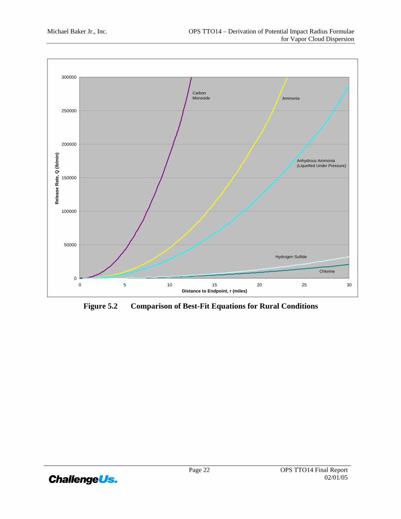
A one-to-one comparison of the best-fit equations for each of the products of interest is presented in Figure 5.2 and Figure 5.3, for rural and urban conditions, respectively.
Michael Baker Jr., Inc. OPS TTO14 – Derivation of Potential Impact Radius Formulae for Vapor Cloud Dispersion
Page 22 OPS TTO14 Final Report
02/01/05
0
50000
100000
150000
200000
250000
300000
0 5 10 15 20 25 30Distance to Endpoint, r (miles)
Rel
ease
Rat
e, Q
(lb/
min
)
Chlorine
Hydrogen Sulfide
Anhydrous Ammonia(Liquefied Under Pressure)
AmmoniaCarbonMonoxide
Figure 5.2 Comparison of Best-Fit Equations for Rural Conditions

Michael Baker Jr., Inc. OPS TTO14 – Derivation of Potential Impact Radius Formulae for Vapor Cloud Dispersion
Page 23 OPS TTO14 Final Report
02/01/05
0
50000
100000
150000
200000
250000
300000
0 5 10 15 20 25 30Distance to Endpoint, r (miles)
Rel
ease
Rat
e, Q
(lb/
min
)
Chlorine
Hydrogen Sulfide
Anhydrous Ammonia(Liquefied Under Pressure)
AmmoniaCarbonMonoxide
Figure 5.3 Comparison of Best-Fit Equations for Urban Conditions
Michael Baker Jr., Inc. OPS TTO14 – Derivation of Potential Impact Radius Formulae for Vapor Cloud Dispersion
Page 24 OPS TTO14 Final Report
02/01/05
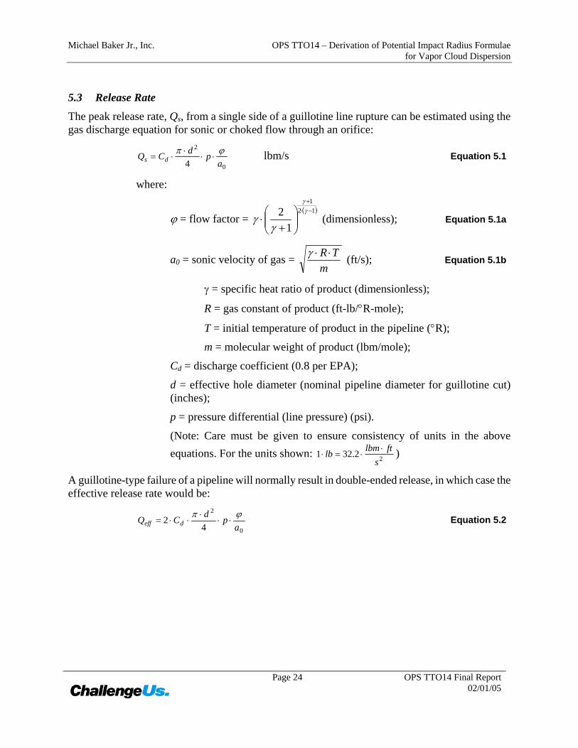
5.3 Release Rate
The peak release rate, Qs, from a single side of a guillotine line rupture can be estimated using the gas discharge equation for sonic or choked flow through an orifice:
0
2
4 apdCQ ds
ϕπ⋅⋅
⋅⋅= lbm/s Equation 5.1
where:
ϕ = flow factor = ( )12
1
12 −⋅
+
⎟⎟⎠
⎞⎜⎜⎝
⎛+
⋅γ
γ
γγ (dimensionless); Equation 5.1a
a0 = sonic velocity of gas = m
TR ⋅⋅γ (ft/s); Equation 5.1b
γ = specific heat ratio of product (dimensionless);
R = gas constant of product (ft-lb/°R-mole);
T = initial temperature of product in the pipeline (°R);
m = molecular weight of product (lbm/mole);
Cd = discharge coefficient (0.8 per EPA);
d = effective hole diameter (nominal pipeline diameter for guillotine cut) (inches);
p = pressure differential (line pressure) (psi).
(Note: Care must be given to ensure consistency of units in the above equations. For the units shown: 22.321
sftlbmlb ⋅
⋅=⋅ )
A guillotine-type failure of a pipeline will normally result in double-ended release, in which case the effective release rate would be:
0
2
42
apdCQ deff
ϕπ⋅⋅
⋅⋅⋅= Equation 5.2

Michael Baker Jr., Inc. OPS TTO14 – Derivation of Potential Impact Radius Formulae for Vapor Cloud Dispersion
Page 25 OPS TTO14 Final Report
02/01/05
5.4 PIR Formulae Derivation
The final step in the derivation of PIR formulae was to relate the effective release rate, Qeff, in the best-fit equations to the release rate that would be calculated for a pipeline of a given diameter and operating pressure using Equation 5.2.
Using the general form of the best-fit equation: B
effQAr ⋅= Equation 5.3
where:
A and B are constants;
Qeff = release rate (lbm/min); and
r = PIR (miles),
and substituting Equation 5.2 for Qeff, yields an equation of the form: B
d apdCAr ⎟
⎟⎠
⎞⎜⎜⎝
⎛⋅⋅
⋅⋅⋅⋅=
0
2
42 ϕπ Equation 5.4
However, since the units of Q in Equation 5.2 are pounds (mass) per second (lbm/s), the quantity within the parentheses must be multiplied by 60 to convert to units required for Equation 5.3, pounds (mass) per minute (lbm/min). As discussed in the note after Equation 5.2, an additional factor of 32.2 must be placed within the parentheses for unit consistency (convert from pounds (force) to pounds (mass)). Thus, the equation becomes:
B
d apdCAr ⎟
⎟⎠
⎞⎜⎜⎝
⎛⋅⋅
⋅⋅⋅⋅⋅⋅=
0
2
42.32602 ϕπ or,
B
d apdCAr ⎟⎟
⎠
⎞⎜⎜⎝
⎛⋅⋅⋅⋅⋅=
0
28.3034 ϕ Equation 5.5

Michael Baker Jr., Inc. OPS TTO14 – Derivation of Potential Impact Radius Formulae for Vapor Cloud Dispersion
Page 26 OPS TTO14 Final Report
02/01/05
5.4.1 Anhydrous Ammonia Calculations
The factors required to develop a PIR formula for anhydrous ammonia using Equation 5.5 are summarized in Table 5.2.
Table 5.2 Factors for Anhydrous Ammonia
Factor Value
Sonic velocity (ft/sec), a0, = mRTγ 1422.9
Rural Conditions 0.073 Constant, A
Urban Conditions 0.064 Rural Conditions 0.48
Constant, B Urban Conditions 0.5
Discharge coefficient (dimensionless), Cd 0.8 Molecular Weight (lbm/lb-mole), m 17.03
Gas Constant (ft-lbf/lb-mole-°R), R 1523
Gas Temperature (°R), T 536.7
Specific Heat Ratio (dimensionless), γ 1.31
Flow Factor (dimensionless), ϕ = ( )121
12 −⋅
+
⎟⎟⎠
⎞⎜⎜⎝
⎛+
⋅γ
γ
γγ 0.77
Substituting these factors into Equation 5.5 yields: 48.0
2
9.142277.08.08.3034073.0 ⎟
⎠⎞
⎜⎝⎛ ⋅⋅⋅⋅⋅= pdr ⇒
( ) 48.02314.1073.0 pdr ⋅⋅⋅= ⇒
( ) 48.0208.0 pdr ⋅⋅= for Rural conditions and, Equation 5.6
45.02
9.142277.08.08.3034064.0 ⎟
⎠⎞
⎜⎝⎛ ⋅⋅⋅⋅⋅= pdr ⇒
( ) 45.02314.1064.0 pdr ⋅⋅⋅= ⇒
( ) 45.0207.0 pdr ⋅⋅= for Urban conditions and, Equation 5.7
5.4.2 Carbon Monoxide Calculations
The factors required to develop a PIR formula for carbon monoxide using Equation 5.5 are summarized in Table 5.3. The tables in the EPA RMP guidance document for neutrally buoyant gases have a slightly different form than the other tables in that the value required to determine the distance to the endpoint is flow rate in lbm/min divided by the toxic endpoint in milligrams per liter

Michael Baker Jr., Inc. OPS TTO14 – Derivation of Potential Impact Radius Formulae for Vapor Cloud Dispersion
Page 27 OPS TTO14 Final Report
02/01/05
(mg/L). Thus, since carbon monoxide is considered neutrally buoyant, the quantity within the parentheses in Equation 5.5 must be divided by the toxic endpoint of 1.725 mg/L.
Table 5.3 Factors for Carbon Monoxide
Factor Value
Sonic velocity (ft/sec), a0, = mRTγ 1154.8
Rural Conditions 0.044 Constant, A
Urban Conditions 0.025 Rural Conditions 0.5
Constant, B Urban Conditions 0.47
Discharge coefficient (dimensionless), Cd 0.8 Molecular Weight (lbm/lb-mole), m 28.01
Gas Constant (ft-lbf/lb-mole-°R), R 1544
Gas Temperature (°R), T 536.7
Specific Heat Ratio (dimensionless), γ 1.40
Flow Factor (dimensionless), ϕ = ( )121
12 −⋅
+
⎟⎟⎠
⎞⎜⎜⎝
⎛+
⋅γ
γ
γγ 0.81
Substituting these factors into Equation 5.5 yields: 5.0
2
725.11
8.115481.08.08.3034044.0 ⎟
⎠⎞
⎜⎝⎛ ⋅⋅⋅⋅⋅⋅= pdr ⇒
( ) 5.02987.0044.0 pdr ⋅⋅⋅= ⇒
( ) 5.0204.0 pdr ⋅⋅= for Rural conditions and, Equation 5.8
45.02
725.11
8.115481.08.08.3034025.0 ⎟
⎠⎞
⎜⎝⎛ ⋅⋅⋅⋅⋅⋅= pdr ⇒
( ) 45.02987.0025.0 pdr ⋅⋅⋅= ⇒
( ) 45.0203.0 pdr ⋅⋅= for Urban conditions and, Equation 5.9
Michael Baker Jr., Inc. OPS TTO14 – Derivation of Potential Impact Radius Formulae for Vapor Cloud Dispersion
Page 28 OPS TTO14 Final Report
02/01/05
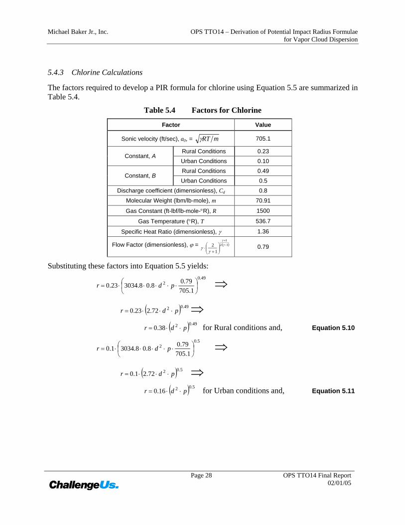
5.4.3 Chlorine Calculations
The factors required to develop a PIR formula for chlorine using Equation 5.5 are summarized in Table 5.4.
Table 5.4 Factors for Chlorine
Factor Value
Sonic velocity (ft/sec), a0, = mRTγ 705.1
Rural Conditions 0.23 Constant, A
Urban Conditions 0.10 Rural Conditions 0.49
Constant, B Urban Conditions 0.5
Discharge coefficient (dimensionless), Cd 0.8 Molecular Weight (lbm/lb-mole), m 70.91
Gas Constant (ft-lbf/lb-mole-°R), R 1500
Gas Temperature (°R), T 536.7
Specific Heat Ratio (dimensionless), γ 1.36
Flow Factor (dimensionless), ϕ = ( )121
12 −⋅
+
⎟⎟⎠
⎞⎜⎜⎝
⎛+
⋅γ
γ
γγ 0.79
Substituting these factors into Equation 5.5 yields: 49.0
2
1.70579.08.08.303423.0 ⎟
⎠⎞
⎜⎝⎛ ⋅⋅⋅⋅⋅= pdr ⇒
( ) 49.0272.223.0 pdr ⋅⋅⋅= ⇒
( ) 49.0238.0 pdr ⋅⋅= for Rural conditions and, Equation 5.10
5.02
1.70579.08.08.30341.0 ⎟
⎠⎞
⎜⎝⎛ ⋅⋅⋅⋅⋅= pdr ⇒
( ) 5.0272.21.0 pdr ⋅⋅⋅= ⇒
( ) 5.0216.0 pdr ⋅⋅= for Urban conditions and, Equation 5.11

Michael Baker Jr., Inc. OPS TTO14 – Derivation of Potential Impact Radius Formulae for Vapor Cloud Dispersion
Page 29 OPS TTO14 Final Report
02/01/05
5.4.4 Hydrogen Sulfide Calculations
The factors required to develop a PIR formula for hydrogen sulfide using Equation 5.5 are summarized in Table 5.5.
Table 5.5 Factors for Hydrogen Sulfide
Factor Value
Sonic velocity (ft/sec), a0, = mRTγ 1010.7
Rural Conditions 0.284 Constant, A
Urban Conditions 0.20 Rural Conditions 0.45
Constant, B Urban Conditions 0.46
Discharge coefficient (dimensionless), Cd 0.8 Molecular Weight (lbm/lb-mole), m 34.08
Gas Constant (ft-lbf/lb-mole-°R), R 1526
Gas Temperature (°R), T 536.7
Specific Heat Ratio (dimensionless), γ 1.32
Flow Factor (dimensionless), ϕ = ( )121
12 −⋅
+
⎟⎟⎠
⎞⎜⎜⎝
⎛+
⋅γ
γ
γγ 0.77
Substituting these factors into Equation 5.5 yields: 45.0
2
7.101077.08.08.303428.0 ⎟
⎠⎞
⎜⎝⎛ ⋅⋅⋅⋅⋅= pdr ⇒
( ) 45.02850.128.0 pdr ⋅⋅⋅= ⇒
( ) 45.0237.0 pdr ⋅⋅= for Rural conditions and, Equation 5.12
46.02
7.101077.08.08.30342.0 ⎟
⎠⎞
⎜⎝⎛ ⋅⋅⋅⋅⋅= pdr ⇒
( ) 46.02850.12.0 pdr ⋅⋅⋅= ⇒
( ) 46.0227.0 pdr ⋅⋅= for Urban conditions and, Equation 5.13
5.5 Formulae Limitations
As mentioned above, the tables presented in the EPA RMP guidance document are based on a 10-minute release duration, thus the PIR formulae derived herein are also based on this release duration. The PIR formulae are also based on the peak release rate from a single side of a guillotine break, whereas the derivation of the PIR formula given in 49 CFR 192 is based on flow from both sides with the application of a decay rate factor. The decay rate factor was applied to acknowledge that the

Michael Baker Jr., Inc. OPS TTO14 – Derivation of Potential Impact Radius Formulae for Vapor Cloud Dispersion
Page 30 OPS TTO14 Final Report
02/01/05
release rate will decline rapidly as the system depressurizes. While the use of a decay rate factor is appropriate when considering the potential impact from a jet fire, it is not appropriate when considering release of a toxic gas, since the potential impact is related to the total quantity released. The following example demonstrates what a 10-minute release at the peak release rate means in terms of actual length of pipeline evacuated.
5.5.1 Toxic Gas Release Example
Assuming an NPS 8 hydrogen sulfide pipeline operating at 1,000 psi and substituting the appropriate values from Table 5.5 into Equation 5.2, the peak release rate is calculated as 118,500 pounds (mass) per minute. Multiplying the release rate by the 10-minute duration of the release results in a total release of 1,185,000 pound (mass).
Dividing this quantity by the quantity in one foot of pipeline (~2.1 lbm/ft) shows that, in this example, the 10-minute release is equivalent to completely venting more than 100 miles of pipeline.

Michael Baker Jr., Inc. OPS TTO14 – Derivation of Potential Impact Radius Formulae for Vapor Cloud Dispersion
Page 31 OPS TTO14 Final Report
02/01/05
6 Development of Simplified PIR Formulae – Flammable Vapor Cloud 6.1 Overview
In the absence of more sophisticated modeling software, a simplified technique for determining the PIR for delayed ignition of a flammable vapor cloud is desired. This technique should account for, at a minimum:
• the physical properties of the gas,
• the maximum operating pressure, and
• the pipeline diameter.
The worse-case scenario for flammable gases given in Risk Management Program Guidance for Offsite Consequence Analysis (EPA 1999) is based on detonation of the total amount of gas that could be released from a pipeline. The impact radius from the detonation is the maximum distance from the source that would experience an overpressure of 1 psi. This basis was chosen “as the threshold for potential serious injuries to people as a result of property damage caused by an explosion (e.g., injuries from flying glass from shattered windows or falling debris from damaged houses).”
Similar to the guidance given in the EPA document for toxic gases, “lookup” tables are provide to determine the distance to the 1 psi overpressure for flammable gases based for various quantities released. The program RMP*Comp discussed in Section 5.1 can also be utilized for analyzing the impacts for flammable gases.
The simplified modeling technique described below is based on the EPA worst-case scenario using a steady state release rate equal to the peak release rate from the rupture. Assuming a 10-minute release at the peak release rate provides a rough estimate of the total quantity released since pipeline “shutdown” after rupture should occur quickly. The release rate will then decay rapidly as the line depressurizes even though the actual total release time may be significantly longer than 10-minutes.
6.2 PIR Formulae Derivation
Appendix C of the EPA guidance document provides equations for estimating the distance to the 1 psi overpressure based on a TNT-equivalency method and assuming that 10 percent of the flammable vapor in the cloud participates in the explosion. The equation (in imperial unit) is given as:
31
1.00081.0 ⎟⎟⎠
⎞⎜⎜⎝
⎛⋅⋅⋅=
TNT
flb HC
HCWr Equation 6.1
where:
r = distance to 1 psi overpressure (miles);
HCf = heat of combustion of gas (BTU/lbm);
HCTNT = heat of explosion of TNT (2,020 BTU/lbm); and

Michael Baker Jr., Inc. OPS TTO14 – Derivation of Potential Impact Radius Formulae for Vapor Cloud Dispersion
Page 32 OPS TTO14 Final Report
02/01/05
Wlb = weight of gas (lbm).
As stated above, the total weight of gas released (Wlb) is taken as a 10-minute release period at the peak release rate (Qeff from Equation 5.2). Thus, the equation becomes:
31
0
2
4210602.321.00081.0 ⎟
⎟⎠
⎞⎜⎜⎝
⎛⋅⋅⋅
⋅⋅⋅⋅⋅⋅⋅⋅=
TNT
fd HC
HCa
pdCrϕπ or,
31
0
20093.0 ⎟⎟⎠
⎞⎜⎜⎝
⎛⋅⋅⋅⋅⋅= fd HC
apdCr
ϕ Equation 6.2
Since the units of Qeff in Equation 5.2 are pounds (mass) per second (lbm/s), a factor of 60 has been added within the parentheses to convert to units for consistency with the stated time of release, 10 minutes. Likewise, an additional factor of 32.2 must be placed within the parentheses for consistency (convert from pounds (force) to pounds (mass)) with the units of pressure.
6.2.1 Acetylene Calculations
The factors required to develop a PIR formula for acetylene using Equation 6.2 are summarized in Table 6.1.
Table 6.1 Factors for Acetylene
Factor Value
Sonic velocity (ft/sec), a0, = mRTγ 1136.6
Discharge coefficient (dimensionless), Cd 0.8 Heat of combustion (BTU/lbm) 20769
Molecular Weight (lbm/lb-mole), m 26.04
Gas Constant (ft-lbf/lb-mole-°R), R 1545
Gas Temperature (°R), T 536.7
Specific Heat Ratio (dimensionless), γ 1.26
Flow Factor (dimensionless), ϕ = ( )121
12 −⋅
+
⎟⎟⎠
⎞⎜⎜⎝
⎛+
⋅γ
γ
γγ 0.74
Substituting these factors into Equation 6.2 yields: 31
2 207696.1136
74.08.00093.0 ⎟⎠⎞
⎜⎝⎛ ⋅⋅⋅⋅⋅= pdr ⇒ ( ) 312818.100093.0 pdr ⋅⋅⋅= ⇒
( ) 312021.0 pdr ⋅⋅= Equation 6.3
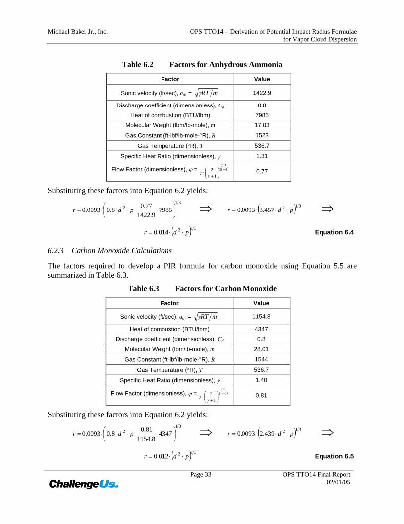
6.2.2 Anhydrous Ammonia Calculations
The factors required to develop a PIR formula for anhydrous ammonia using Equation 6.2 are summarized in Table 6.2.
Michael Baker Jr., Inc. OPS TTO14 – Derivation of Potential Impact Radius Formulae for Vapor Cloud Dispersion
Page 33 OPS TTO14 Final Report
02/01/05
Table 6.2 Factors for Anhydrous Ammonia
Factor Value
Sonic velocity (ft/sec), a0, = mRTγ 1422.9
Discharge coefficient (dimensionless), Cd 0.8 Heat of combustion (BTU/lbm) 7985
Molecular Weight (lbm/lb-mole), m 17.03
Gas Constant (ft-lbf/lb-mole-°R), R 1523
Gas Temperature (°R), T 536.7
Specific Heat Ratio (dimensionless), γ 1.31
Flow Factor (dimensionless), ϕ = ( )121
12 −⋅
+
⎟⎟⎠
⎞⎜⎜⎝
⎛+
⋅γ
γ
γγ 0.77
Substituting these factors into Equation 6.2 yields: 31
2 79859.1422
77.08.00093.0 ⎟⎠⎞
⎜⎝⎛ ⋅⋅⋅⋅⋅= pdr ⇒ ( ) 312457.30093.0 pdr ⋅⋅⋅= ⇒
( ) 312014.0 pdr ⋅⋅= Equation 6.4
6.2.3 Carbon Monoxide Calculations
The factors required to develop a PIR formula for carbon monoxide using Equation 5.5 are summarized in Table 6.3.
Table 6.3 Factors for Carbon Monoxide
Factor Value
Sonic velocity (ft/sec), a0, = mRTγ 1154.8
Heat of combustion (BTU/lbm) 4347 Discharge coefficient (dimensionless), Cd 0.8
Molecular Weight (lbm/lb-mole), m 28.01
Gas Constant (ft-lbf/lb-mole-°R), R 1544
Gas Temperature (°R), T 536.7
Specific Heat Ratio (dimensionless), γ 1.40
Flow Factor (dimensionless), ϕ = ( )121
12 −⋅
+
⎟⎟⎠
⎞⎜⎜⎝
⎛+
⋅γ
γ
γγ 0.81
Substituting these factors into Equation 6.2 yields: 31
2 43478.1154
81.08.00093.0 ⎟⎠⎞
⎜⎝⎛ ⋅⋅⋅⋅⋅= pdr ⇒ ( ) 312439.20093.0 pdr ⋅⋅⋅= ⇒
( ) 312012.0 pdr ⋅⋅= Equation 6.5

Michael Baker Jr., Inc. OPS TTO14 – Derivation of Potential Impact Radius Formulae for Vapor Cloud Dispersion
Page 34 OPS TTO14 Final Report
02/01/05
6.2.4 Ethylene Calculations
The factors required to develop a PIR formula for ethylene using Equation 6.2 are summarized in Table 6.4.
Table 6.4 Factors for Ethylene
Factor Value
Sonic velocity (ft/sec), a0, = mRTγ 1073.8
Heat of combustion (BTU/lbm) 20275 Discharge coefficient (dimensionless), Cd 0.8
Molecular Weight (lbm/lb-mole), m 28.05
Gas Constant (ft-lbf/lb-mole-°R), R 1534
Gas Temperature (°R), T 536.7
Specific Heat Ratio (dimensionless), γ 1.22
Flow Factor (dimensionless), ϕ = ( )121
12 −⋅
+
⎟⎟⎠
⎞⎜⎜⎝
⎛+
⋅γ
γ
γγ 0.72
Substituting these factors into Equation 6.2 yields: 31
2 202758.1073
72.08.00093.0 ⎟⎠⎞
⎜⎝⎛ ⋅⋅⋅⋅⋅= pdr ⇒ ( ) 312876.100093.0 pdr ⋅⋅⋅= ⇒
( ) 312021.0 pdr ⋅⋅= Equation 6.6

Michael Baker Jr., Inc. OPS TTO14 – Derivation of Potential Impact Radius Formulae for Vapor Cloud Dispersion
Page 35 OPS TTO14 Final Report
02/01/05
6.2.5 Hydrogen Sulfide Calculations
The factors required to develop a PIR formula for hydrogen sulfide using Equation 6.2 are summarized in Table 6.5.
Table 6.5 Factors for Hydrogen Sulfide
Factor Value
Sonic velocity (ft/sec), a0, = mRTγ 1010.7
Heat of combustion (BTU/lbm) 6537 Discharge coefficient (dimensionless), Cd 0.8
Molecular Weight (lbm/lb-mole), m 34.08
Gas Constant (ft-lbf/lb-mole-°R), R 1526
Gas Temperature (°R), T 536.7
Specific Heat Ratio (dimensionless), γ 1.32
Flow Factor (dimensionless), ϕ = ( )121
12 −⋅
+
⎟⎟⎠
⎞⎜⎜⎝
⎛+
⋅γ
γ
γγ 0.77
Substituting these factors into Equation 6.2 yields: 31
2 65377.1010
77.08.00093.0 ⎟⎠⎞
⎜⎝⎛ ⋅⋅⋅⋅⋅= pdr ⇒ ( ) 312984.30093.0 pdr ⋅⋅⋅= ⇒
( ) 312015.0 pdr ⋅⋅= Equation 6.7
6.2.6 Methane Calculations
The factors required to develop a PIR formula for methane using Equation 6.2 are summarized in Table 6.6.
Table 6.6 Factors for Methane
Factor Value
Sonic velocity (ft/sec), a0, = mRTγ 1480.0
Heat of combustion (BTU/lbm) 21495 Discharge coefficient (dimensionless), Cd 0.8
Molecular Weight (lbm/lb-mole), m 16.04
Gas Constant (ft-lbf/lb-mole-°R), R 1546
Gas Temperature (°R), T 536.7
Specific Heat Ratio (dimensionless), γ 1.32
Flow Factor (dimensionless), ϕ = ( )121
12 −⋅
+
⎟⎟⎠
⎞⎜⎜⎝
⎛+
⋅γ
γ
γγ 0.77
Substituting these factors into Equation 6.2 yields:

Michael Baker Jr., Inc. OPS TTO14 – Derivation of Potential Impact Radius Formulae for Vapor Cloud Dispersion
Page 36 OPS TTO14 Final Report
02/01/05
312 21495
0.148077.08.00093.0 ⎟
⎠⎞
⎜⎝⎛ ⋅⋅⋅⋅⋅= pdr ⇒ ( ) 312947.80093.0 pdr ⋅⋅⋅= ⇒
( ) 312019.0 pdr ⋅⋅= Equation 6.8
6.2.7 Rich Gas Calculations
The factors required to develop a PIR formula for methane using Equation 6.2 are summarized in Table 6.7.
Table 6.7 Factors for Rich Gas
Factor Value
Sonic velocity (ft/sec), a0, = mRTγ 1330.1
Heat of combustion (BTU/lbm) 20586 Discharge coefficient (dimensionless), Cd 0.8
Molecular Weight (lbm/lb-mole), m 19.488
Gas Constant (ft-lbf/lb-mole-°R), R 1546
Gas Temperature (°R), T 536.7
Specific Heat Ratio (dimensionless), γ 1.29
Flow Factor (dimensionless), ϕ = ( )121
12 −⋅
+
⎟⎟⎠
⎞⎜⎜⎝
⎛+
⋅γ
γ
γγ 0.76
Substituting these factors into Equation 6.2 yields: 31
2 205861.1330
76.08.00093.0 ⎟⎠⎞
⎜⎝⎛ ⋅⋅⋅⋅⋅= pdr ⇒ ( ) 312410.90093.0 pdr ⋅⋅⋅= ⇒
( ) 312020.0 pdr ⋅⋅= Equation 6.9
6.3 Methodology for Flammable Gas Mixtures
The derivation of a PIR formula based on a 1 psi overpressure for a mixture of flammable gases is identical to the process discussed above; however, appropriate values for several of the required parameters must be calculated (molecular weight, specific heat ratio, heat of combustion, etc.).
The molecular weight of a gas mixture can be estimated using the following general formula: ...+⋅+⋅+⋅= zzyyxxmix mFmFmFm Equation 6.10
where:
Fx = fraction of substance x;
Fy = fraction of substance y;
Fz = fraction of substance z;
mx = molecular weight of substance x;

Michael Baker Jr., Inc. OPS TTO14 – Derivation of Potential Impact Radius Formulae for Vapor Cloud Dispersion
Page 37 OPS TTO14 Final Report
02/01/05
my = molecular weight of substance y; and
mz = molecular weight of substance z.
Similarly, the heat of combustion of a gas mixture can be estimated using the following general formula:
mix
CzzzCyyyCxxxmixC m
HmFHmFHmFH
...+⋅⋅+⋅⋅+⋅⋅= Equation 6.11
where:
HCx = heat of combustion of substance x;
HCy = heat of combustion of substance y; and
HCz = heat of combustion of substance z.
Finally, the specific heat ratio weight of a gas mixture can be approximated using the following general formula:
...+⋅+⋅+⋅= zzyyxxmix FFF λλγγ Equation 6.12
where:
γx = specific heat ratio of substance x;
γy = specific heat ratio of substance y; and
γz = specific heat ratio of substance z.
The remaining parameters can then be calculated using Equations 5.1a and 5.1b. The final PIR is then calculated using Equation 6.2.
6.3.1 Example of Mixed Gas Calculations
The following example demonstrates the calculation process for determining the PIR for mixed gas. The composition used (see Table 6.8) is typical of landfill gas. This example is for an NPS 16 pipeline operating at 100 psi.
Table 6.8 Mixed Gas Properties and Composition
Compound Molecular
Weight (lbm/lb-mole)
Specific Heat Ratio
Heat of Combustion
(Btu/lbm)
Composition (%)
Methane 16.04 1.31 21,495 55.0
Nitrogen 28.02 1.40 0 10.0
Carbon Dioxide 44.01 1.30 0 35.0
Substituting the appropriate values from Table 6.8 into Equations 6.10, 6.11 and 6.12 to calculate the molecular weight, specific heat ration and heat of combustion of the mixture gives:
molelblbmmmix −⋅=⋅+⋅+⋅= /03.2701.4435.002.281.004.1655.0 ;

Michael Baker Jr., Inc. OPS TTO14 – Derivation of Potential Impact Radius Formulae for Vapor Cloud Dispersion
Page 38 OPS TTO14 Final Report
02/01/05
32.130.135.040.11.031.155.0 =⋅+⋅+⋅=mixγ ; and
lbmBtuH mixC /015,703.27
001.4435.0002.281.02149504.1655.0⋅=
⋅⋅+⋅⋅+⋅⋅= .
Next, determine the flow factor of the mixed gas by substituting the specific heat ratio into Equation 5.1a:
( )77.0
132.1232.1
132.12132.1
=⎟⎠⎞
⎜⎝⎛
+⋅=
−⋅+
ϕ .
The sonic velocity is calculated using Equation 5.1b. The universal gas constant, R, is normally given as 1,546 ft-lb/lb-mole °F. For this example the gas temperature is assumed to be 59°F (518.4°R).
sfta /6.122,103.27
2.324.518154632.10 ⋅=
⋅⋅⋅= .
[Note: The value 32.2 is the conversion from pound (mass) to pound (force), (1 lbf = 32.2 lbm ft/s2).]
Finally, substituting the appropriate values for all parameters in Equation 6.2 gives a PIR formula of: 31
2 70156.1122
77.08.00093.0 ⎟⎠⎞
⎜⎝⎛ ⋅⋅⋅⋅⋅= pdr ⇒ ( ) 312849.30093.0 pdr ⋅⋅⋅= ⇒
( ) 312015.0 pdr ⋅⋅= Equation 6.9
6.4 Formulae Limitations
As mentioned above, the tables presented in the EPA RMP guidance document are based entirely upon the quantity released. In the derivation of PIR formulae for ignition of a flammable vapor cloud described herein, the total quantity released was calculated as a 10-minute release at the peak release rate from a two-sided guillotine break. In addition, the derivation of the PIR formula given in 49 CFR 192 applied a decay rate factor to acknowledge that the release rate will fall off fairly quickly as the system depressurizes. While the use of a decay rate factor is appropriate when considering the potential impact from a jet fire, it is not appropriate when considering formation of a flammable vapor cloud, since the potential impact is related to the total quantity released.
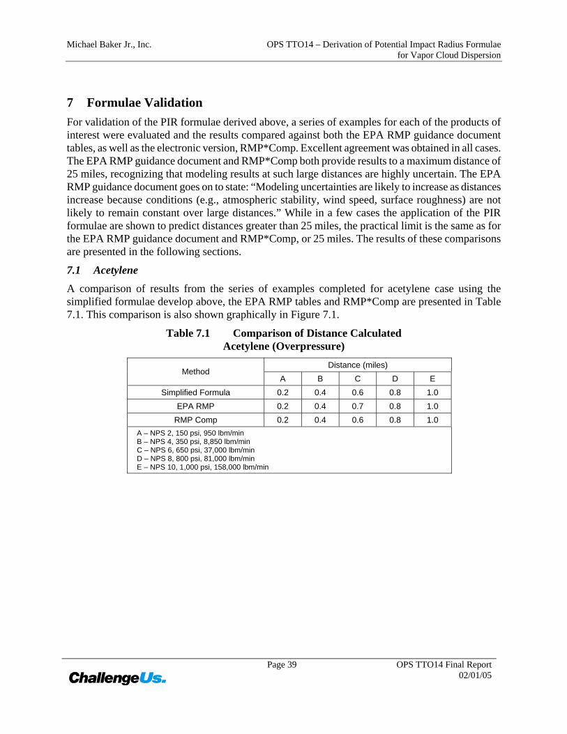
Michael Baker Jr., Inc. OPS TTO14 – Derivation of Potential Impact Radius Formulae for Vapor Cloud Dispersion
Page 39 OPS TTO14 Final Report
02/01/05
7 Formulae Validation For validation of the PIR formulae derived above, a series of examples for each of the products of interest were evaluated and the results compared against both the EPA RMP guidance document tables, as well as the electronic version, RMP*Comp. Excellent agreement was obtained in all cases. The EPA RMP guidance document and RMP*Comp both provide results to a maximum distance of 25 miles, recognizing that modeling results at such large distances are highly uncertain. The EPA RMP guidance document goes on to state: “Modeling uncertainties are likely to increase as distances increase because conditions (e.g., atmospheric stability, wind speed, surface roughness) are not likely to remain constant over large distances.” While in a few cases the application of the PIR formulae are shown to predict distances greater than 25 miles, the practical limit is the same as for the EPA RMP guidance document and RMP*Comp, or 25 miles. The results of these comparisons are presented in the following sections.
7.1 Acetylene
A comparison of results from the series of examples completed for acetylene case using the simplified formulae develop above, the EPA RMP tables and RMP*Comp are presented in Table 7.1. This comparison is also shown graphically in Figure 7.1.
Table 7.1 Comparison of Distance Calculated Acetylene (Overpressure)
Distance (miles) Method
A B C D E Simplified Formula 0.2 0.4 0.6 0.8 1.0
EPA RMP 0.2 0.4 0.7 0.8 1.0 RMP Comp 0.2 0.4 0.6 0.8 1.0
A – NPS 2, 150 psi, 950 lbm/min B – NPS 4, 350 psi, 8,850 lbm/min C – NPS 6, 650 psi, 37,000 lbm/min D – NPS 8, 800 psi, 81,000 lbm/min E – NPS 10, 1,000 psi, 158,000 lbm/min

Michael Baker Jr., Inc. OPS TTO14 – Derivation of Potential Impact Radius Formulae for Vapor Cloud Dispersion
Page 40 OPS TTO14 Final Report
02/01/05
0.0
0.2
0.4
0.6
0.8
1.0
1.2
Dis
tanc
e to
1 p
si O
verp
ress
ure
(mile
s)
Simplif ied Formula EPA RMP RMP*Comp
Figure 7.1 Acetylene – Overpressure
7.2 Anhydrous Ammonia
A comparison of results from the series of examples completed for anhydrous ammonia (liquefied under pressure) case using the simplified formulae develop above, the EPA RMP tables and RMP*Comp are presented in Table 7.2 and Table 7.3 for rural and urban conditions, respectively. This comparison is also shown graphically in Figure 7.2 and Figure 7.3.
Table 7.2 Comparison of Distance Calculated Anhydrous Ammonia (Rural Conditions)
Distance (miles) Method
A B C D E Simplified Formula 5.0 10.0 16.2 22.4 28.9
EPA RMP 4.9 9.7 18.0 >25 >25 RMP Comp 4.9 9.7 15.0 22 >25
SLAB 3.6 8.8 14.0 — — A – NPS 4, 350 psi, 7,300 lbm/min B – NPS 6, 650 psi, 30,600 lbm/min C – NPS 8, 1,000 psi, 83,600 lbm/min D – NPS 10, 1,250 psi, 163,300 lbm/min E – NPS 12, 1,480 psi, 278,500 lbm/min

Michael Baker Jr., Inc. OPS TTO14 – Derivation of Potential Impact Radius Formulae for Vapor Cloud Dispersion
Page 41 OPS TTO14 Final Report
02/01/05
Table 7.3 Comparison of Distance Calculated Anhydrous Ammonia (Urban Conditions)
Method Distance (miles) Simplified Formula 3.4 6.5 10.2 13.8 17.5
EPA RMP 3.2 6.1 10.0 15.0 >25 RMP Comp 3.2 6.1 9.5 13.0 17.0
A – NPS 4, 350 psi, 7,300 lbm/min B – NPS 6, 650 psi, 30,600 lbm/min C – NPS 8, 1,000 psi, 83,600 lbm/min D – NPS 10, 1,250 psi, 163,300 lbm/min E – NPS 12, 1,480 psi, 278,500 lbm/min
0.0
2.0
4.0
6.0
8.0
10.0
12.0
14.0
16.0
18.0
20.0
22.0
24.0
Dis
tanc
e to
End
poin
t (m
iles)
Simplif ied Formula EPA RMP RMP Comp SLAB
Figure 7.2 Anhydrous Ammonia – Rural Conditions

Michael Baker Jr., Inc. OPS TTO14 – Derivation of Potential Impact Radius Formulae for Vapor Cloud Dispersion
Page 42 OPS TTO14 Final Report
02/01/05
Urban Conditions
0.0
2.0
4.0
6.0
8.0
10.0
12.0
14.0
16.0
18.0
20.0
Dis
tanc
e to
End
poin
t (m
iles)
Simplif ied Formula EPA RMP RMP Comp
Figure 7.3 Anhydrous Ammonia – Urban Conditions
7.3 Carbon Monoxide
A comparison of results from the series of examples completed for carbon monoxide case using the simplified formulae develop above, the EPA RMP tables and RMP*Comp are presented in Table 7.4 and Table 7.5 for rural and urban conditions, respectively. This comparison is also shown graphically in Figure 7.4 and Figure 7.5.
Table 7.4 Comparison of Distance Calculated Carbon Monoxide (Rural Conditions)
Distance (miles) Method
A B C D E Simplified Formula 3.0 6.1 10.1 14.1 18.5
EPA RMP 2.8 5.6 9.3 14.0 19.0 RMP Comp NA NA NA NA NA
A – NPS 4, 350 psi, 9,500 lbm/min B – NPS 6, 650 psi, 39,900 lbm/min C – NPS 8, 1,000 psi, 109,000 lbm/min D – NPS 10, 1,250 psi, 213,000 lbm/min E – NPS 12, 1,480 psi, 363,000 lbm/min
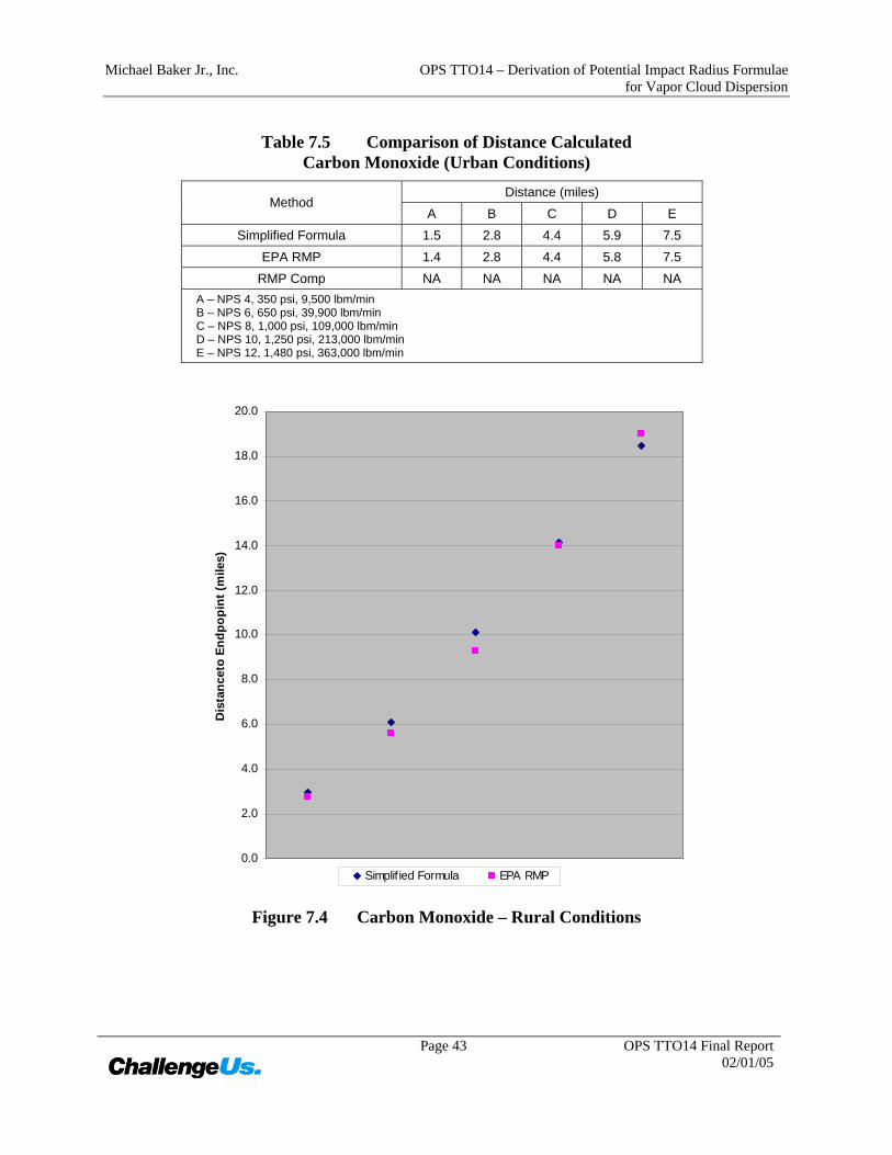
Michael Baker Jr., Inc. OPS TTO14 – Derivation of Potential Impact Radius Formulae for Vapor Cloud Dispersion
Page 43 OPS TTO14 Final Report
02/01/05
Table 7.5 Comparison of Distance Calculated Carbon Monoxide (Urban Conditions)
Distance (miles) Method
A B C D E Simplified Formula 1.5 2.8 4.4 5.9 7.5
EPA RMP 1.4 2.8 4.4 5.8 7.5 RMP Comp NA NA NA NA NA
A – NPS 4, 350 psi, 9,500 lbm/min B – NPS 6, 650 psi, 39,900 lbm/min C – NPS 8, 1,000 psi, 109,000 lbm/min D – NPS 10, 1,250 psi, 213,000 lbm/min E – NPS 12, 1,480 psi, 363,000 lbm/min
0.0
2.0
4.0
6.0
8.0
10.0
12.0
14.0
16.0
18.0
20.0
Dis
tanc
eto
Endp
opin
t (m
iles)
Simplif ied Formula EPA RMP
Figure 7.4 Carbon Monoxide – Rural Conditions

Michael Baker Jr., Inc. OPS TTO14 – Derivation of Potential Impact Radius Formulae for Vapor Cloud Dispersion
Page 44 OPS TTO14 Final Report
02/01/05
Urban Conditions
0.0
1.0
2.0
3.0
4.0
5.0
6.0
7.0
8.0
Dis
tanc
e to
End
poin
t (m
iles)
Simplif ied Formula EPA RMP
Figure 7.5 Carbon Monoxide – Urban Conditions
7.4 Chlorine
A comparison of results from the series of examples completed for chlorine case using the simplified formulae develop above, the EPA RMP tables and RMP*Comp are presented in Table 7.6 and Table 7.7 for rural and urban conditions, respectively. This comparison is also shown graphically in Figure 7.6 and Figure 7.7.
Table 7.6 Comparison of Distance Calculated Chlorine (Rural Conditions)
Distance (miles) Method
A B Simplified Formula 13.2 35.3
EPA RMP 13.0 >25 RMP Comp 13.0 >25
SLAB 8.7 24.8 A – NPS 2, 350 psi, 3,800 lbm/min B – NPS 4, 650 psi, 28,300 lbm/min
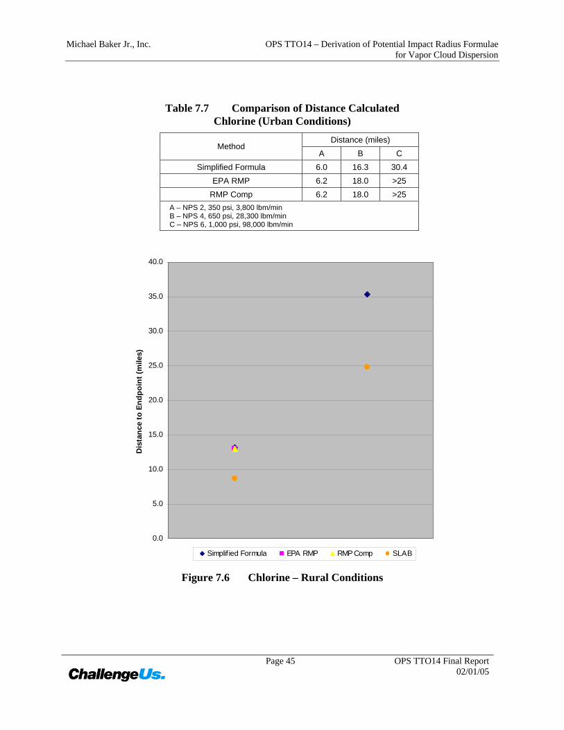
Michael Baker Jr., Inc. OPS TTO14 – Derivation of Potential Impact Radius Formulae for Vapor Cloud Dispersion
Page 45 OPS TTO14 Final Report
02/01/05
Table 7.7 Comparison of Distance Calculated Chlorine (Urban Conditions)
Distance (miles) Method
A B C Simplified Formula 6.0 16.3 30.4
EPA RMP 6.2 18.0 >25 RMP Comp 6.2 18.0 >25
A – NPS 2, 350 psi, 3,800 lbm/min B – NPS 4, 650 psi, 28,300 lbm/min C – NPS 6, 1,000 psi, 98,000 lbm/min
0.0
5.0
10.0
15.0
20.0
25.0
30.0
35.0
40.0
Dis
tanc
e to
End
poin
t (m
iles)
Simplif ied Formula EPA RMP RMP Comp SLAB
Figure 7.6 Chlorine – Rural Conditions
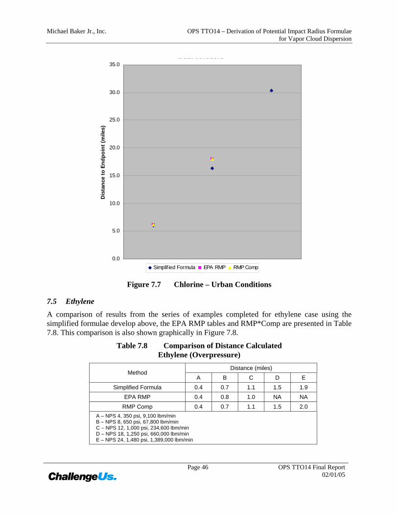
Michael Baker Jr., Inc. OPS TTO14 – Derivation of Potential Impact Radius Formulae for Vapor Cloud Dispersion
Page 46 OPS TTO14 Final Report
02/01/05
Urban Conditions
0.0
5.0
10.0
15.0
20.0
25.0
30.0
35.0
Dis
tanc
e to
End
poin
t (m
iles)
Simplif ied Formula EPA RMP RMP Comp
Figure 7.7 Chlorine – Urban Conditions
7.5 Ethylene
A comparison of results from the series of examples completed for ethylene case using the simplified formulae develop above, the EPA RMP tables and RMP*Comp are presented in Table 7.8. This comparison is also shown graphically in Figure 7.8.
Table 7.8 Comparison of Distance Calculated Ethylene (Overpressure)
Distance (miles) Method
A B C D E Simplified Formula 0.4 0.7 1.1 1.5 1.9
EPA RMP 0.4 0.8 1.0 NA NA RMP Comp 0.4 0.7 1.1 1.5 2.0
A – NPS 4, 350 psi, 9,100 lbm/min B – NPS 8, 650 psi, 67,800 lbm/min C – NPS 12, 1,000 psi, 234,600 lbm/min D – NPS 18, 1,250 psi, 660,000 lbm/min E – NPS 24, 1,480 psi, 1,389,000 lbm/min

Michael Baker Jr., Inc. OPS TTO14 – Derivation of Potential Impact Radius Formulae for Vapor Cloud Dispersion
Page 47 OPS TTO14 Final Report
02/01/05
0.0
0.2
0.4
0.6
0.8
1.0
1.2
1.4
1.6
1.8
2.0
2.2
Dis
tanc
e to
1 p
si O
verp
ress
ure
(mile
s)
Simplif ied Formula EPA RMP RMP*Comp
Figure 7.8 Ethylene – Overpressure
7.6 Hydrogen Sulfide
A comparison of results from the series of examples completed for hydrogen sulfide case using the simplified formulae develop above, the EPA RMP tables and RMP*Comp are presented in Table 7.9 and Table 7.10 for rural and urban conditions, respectively. This comparison is also shown graphically in Figure 7.9 and Figure 7.10.
Table 7.9 Comparison of Distance Calculated Hydrogen Sulfide (Rural Conditions)
Distance (miles) Method
A B C Simplified Formula 9.4 23.1 40.4
EPA RMP 8.7 19.0 >25 RMP Comp 9.3 23.0 >25
SLAB 3.7 10.4 — A – NPS 2, 350 psi, 2,600 lbm/min B – NPS 4, 650 psi, 19,300 lbm/min C – NPS 6, 1,000 psi, 66,700 lbm/min

Michael Baker Jr., Inc. OPS TTO14 – Derivation of Potential Impact Radius Formulae for Vapor Cloud Dispersion
Page 48 OPS TTO14 Final Report
02/01/05
Table 7.10 Comparison of Distance Calculated Hydrogen Sulfide (Urban Conditions)
Distance (miles) Method
A B C Simplified Formula 7.6 19.0 33.7
EPA RMP 6.2 15.0 >25 RMP Comp 6.8 19.0 >25
A – NPS 2, 350 psi, 2,600 lbm/min B – NPS 4, 650 psi, 19,300 lbm/min C – NPS 6, 1,000 psi, 66,700 lbm/min
0.0
5.0
10.0
15.0
20.0
25.0
30.0
35.0
40.0
45.0
Dis
tanc
e to
End
poin
t (m
iles)
Simplif ied Formula EPA RMP RMP Comp SLAB
Figure 7.9 Hydrogen Sulfide – Rural Conditions

Michael Baker Jr., Inc. OPS TTO14 – Derivation of Potential Impact Radius Formulae for Vapor Cloud Dispersion
Page 49 OPS TTO14 Final Report
02/01/05
0.0
5.0
10.0
15.0
20.0
25.0
30.0
35.0
40.0
Dis
tanc
e to
End
poin
t (m
iles)
Simplif ied Formula EPA RMP RMP Comp
Figure 7.10 Hydrogen Sulfide – Urban Conditions
7.7 Methane
A comparison of results from a series of examples completed for methane case using the simplified formulae develop above, the EPA RMP tables and RMP*Comp are presented in Table 7.11. This comparison is also shown graphically in Figure 7.11.
Table 7.11 Comparison of Distance Calculated Methane (Overpressure)
Distance (miles) Method
A B C D E Simplified Formula 0.3 0.6 1.0 1.4 1.7
EPA RMP 0.3 0.6 1.1 1.4 NA RMP Comp 0.3 0.6 1.0 1.4 1.7
A – NPS 4, 350 psi, 7,000 lbm/min B – NPS 8, 650 psi, 52,400 lbm/min C – NPS 12, 1,000 psi, 181,500 lbm/min D – NPS 18, 1,250 psi, 510,400 lbm/min E – NPS 24, 1,480 psi, 1,074,400 lbm/min

Michael Baker Jr., Inc. OPS TTO14 – Derivation of Potential Impact Radius Formulae for Vapor Cloud Dispersion
Page 50 OPS TTO14 Final Report
02/01/05
0.0
0.2
0.4
0.6
0.8
1.0
1.2
1.4
1.6
1.8
2.0
Dis
tanc
e to
1 p
si O
verp
ress
ure
(mile
s)
Simplif ied Formula EPA RMP RMP*Comp
Figure 7.11 Methane – Overpressure

Michael Baker Jr., Inc. OPS TTO14 – Derivation of Potential Impact Radius Formulae for Vapor Cloud Dispersion
Page 51 OPS TTO14 Final Report
02/01/05
8 Conclusions Following the procedures discussed above based on EPA RMP guidance documents, PIR formulae for toxic cloud dispersion and/or 1 psi overpressure were developed for acetylene, anhydrous ammonia (liquefied under pressure), carbon monoxide, chlorine, ethylene, hydrogen sulfide, methane, and rich gas. The recommended formulae are summarized in Table 8.1.
Table 8.1 Summary of PIR Formulae
Product PIR Formula
Acetylene 1 psi Overpressure ( ) 312021.0 pdr ⋅⋅=
1 psi Overpressure ( ) 312014.0 pdr ⋅⋅=
Rural Conditions ( ) 48.0208.0 pdr ⋅⋅= Anhydrous Ammonia (Liquefied under pressure)
Urban Conditions ( ) 45.0207.0 pdr ⋅⋅=
1 psi Overpressure ( ) 312012.0 pdr ⋅⋅=
Rural Conditions ( ) 5.0204.0 pdr ⋅⋅= Carbon Monoxide
Urban Conditions ( ) 45.0203.0 pdr ⋅⋅=
Rural Conditions ( ) 49.0238.0 pdr ⋅⋅= Chlorine
Urban Conditions ( ) 5.0216.0 pdr ⋅⋅=
Ethylene 1 psi Overpressure ( ) 312021.0 pdr ⋅⋅=
1 psi Overpressure ( ) 312015.0 pdr ⋅⋅=
Rural Conditions ( ) 45.0237.0 pdr ⋅⋅= Hydrogen Sulfide
Urban Conditions ( ) 46.0227.0 pdr ⋅⋅=
Methane 1 psi Overpressure ( ) 312019.0 pdr ⋅⋅=
Rich Gas 1 psi Overpressure ( ) 312020.0 pdr ⋅⋅=
There are two differences between the way the release rate is applied in the derivations described in this report and how the release rate was applied in the original formulation of the PIR formula referenced in 49 CFR 192. First, in this report, the peak release rate is assumed to be unabated for the full ten-minute release duration, where the original formula accounted for the rapid decay in release rate as the system depressurizes by applying a release rate decay factor in the derivation. Since the total quantity released is the main concern when dealing with toxic gases, the application of a release rate decay factor is not appropriate. The second difference is the value of the discharge

Michael Baker Jr., Inc. OPS TTO14 – Derivation of Potential Impact Radius Formulae for Vapor Cloud Dispersion
Page 52 OPS TTO14 Final Report
02/01/05
coefficient used in calculating the release rate. A factor of 0.8 was used in this report to be consistent with the EPA RMP guidance document compared to the 0.62 factor used in deriving the PIR formula given in 49 CFR 192.
Michael Baker Jr., Inc. OPS TTO14 – Derivation of Potential Impact Radius Formulae for Vapor Cloud Dispersion
Page 53 OPS TTO14 Final Report
02/01/05
9 References EPA. 1999. Risk Management Program Guidance for Offsite Consequence Analysis.
Office of Pipeline Safety website; http://ops.dot.gov/stats.htm; Liquid Pipeline Accident Yearly Summaries.
Stephens, M.J. 2000. A Model for Sizing High Consequence Areas Associated with Natural Gas Pipelines. GRI-00/0189, October.

Michael Baker Jr., Inc. OPS TTO14 – Derivation of Potential Impact Radius Formulae for Vapor Cloud Dispersion
Page 54 OPS TTO14 Final Report
02/01/05
This page intentionally left blank
Michael Baker Jr., Inc. OPS TTO14 – Derivation of Potential Impact Radius Formulae for Vapor Cloud Dispersion
Page 1 OPS TTO14 Final Report
02/01/05
Appendix A Information from the EPA TTN SCRAM Website

Michael Baker Jr., Inc. OPS TTO14 – Derivation of Potential Impact Radius Formulae for Vapor Cloud Dispersion
Page 2 OPS TTO14 Final Report
02/01/05
This page intentionally left blank

Michael Baker Jr., Inc. OPS TTO14 – Derivation of Potential Impact Radius Formulae for Vapor Cloud Dispersion
Page 3 OPS TTO14 Final Report
02/01/05
The following information is a reproduction of the information on Preferred/Recommended Models presented at the US EPA TTN SCRAM Dispersion Models website:
(http://www.epa.gov/scram001/tt22.htm).
Note that the majority of the models are NOT applicable for determining an air toxic end point resulting from a pipeline rupture. This information, along with the information presented in Appendices B and C, was reviewed as part of this study with the modeling software deemed appropriate for use in analyzing the potential impact of a hazardous/toxic gas release due to pipeline rupture being summarized in Section 0.
Preferred/Recommended Models: The models listed in this area are currently listed in Appendix A of the Guideline on Air Quality Models (published as Appendix W of 40 CFR Part 51). See Appendix A of the Guideline, posted on the Modeling Guidance page of this website for a summary description of these models: BLP, CALINE3, CALPUFF, CTDMPLUS, ISC3, and OCD.
• BLP (Buoyant Line and Point Source Model): a Gaussian plume dispersion model designed to handle unique modeling problems associated with aluminum reduction plants, and other industrial sources where plume rise and downwash effects from stationary line sources are important.
• CALINE3: a steady-state Gaussian dispersion model designed to determine air pollution concentrations at receptor locations downwind of "at-grade," "fill," "bridge," and "cut section" highways located in relatively uncomplicated terrain.
• CALPUFF: a multi-layer, multi-species non-steady-state puff dispersion model that simulates the effects of time- and space-varying meteorological conditions on pollution transport, transformation and removal. CALPUFF can be applied on scales of tens to hundreds of kilometers. It includes algorithms for sub grid scale effects (such as terrain impingement), as well as, longer-range effects (such as pollutant removal due to wet scavenging and dry deposition, chemical transformation, and visibility effects of particulate matter concentrations).
• CTDMPLUS (Complex Terrain Dispersion Model Plus Algorithms for Unstable Situations): a refined point source gaussian air quality model for use in all stability conditions for complex terrain. The model contains, in its entirety, the technology of CTDM for stable and neutral conditions.
• ISC3 (Industrial Source Complex Model): a steady-state Gaussian plume model, which can be used to assess pollutant concentrations from a wide variety of sources associated with an industrial complex. This model can account for the following: settling and dry deposition of particles; downwash; point, area, line, and volume sources; plume rise as a function of downwind distance; separation of point sources; and limited terrain adjustment. ISC3 operates in both long-term and short-term modes.

Michael Baker Jr., Inc. OPS TTO14 – Derivation of Potential Impact Radius Formulae for Vapor Cloud Dispersion
Page 4 OPS TTO14 Final Report
02/01/05
• OCD (Offshore and Coastal Dispersion Model): a straight line Gaussian model developed to determine the impact of offshore emissions from point, area or line sources on the air quality of coastal regions. OCD incorporates over water plume transport and dispersion as well as changes that occur as the plume crosses the shoreline. Hourly meteorological data are needed from both offshore and onshore locations.
Screening Tools: This area provides a list of screening tools that can be used proceeding a refined modeling analysis. The screening tools listed in this section are: CAL3QHC/CAL3QHCR, COMPLEX1, CTSCREEN, LONGZ, RTDM3.2, SCREEN3, SHORTZ, TSCREEN, VALLEY, and VISCREEN.
• CAL3QHC/CAL3QHCR (CALINE3 with queuing and hot spot calculations): CAL3QHC is a CALINE3 based CO model with a traffic model to calculate delays and queues that occur at signalized intersections; CAL3QHCR is a more refined version based on CAL3QHC that requires local meteorological data. Both models are available below.
• COMPLEX1: a multiple point source screening technique with terrain adjustment that incorporates the plume impaction algorithm of the VALLEY model.
• CTSCREEN (Complex Terrain Screening model): a Gaussian plume dispersion model designed as a screening technique for regulatory application to plume impaction assessments in complex terrain. CTSCREEN is a screening version of the CTDMPLUS model.
• LONGZ: a steady-state Gaussian plume formulation for both urban and rural areas in flat or complex terrain to calculate long term (seasonal and/or annual) ground-level ambient air concentrations attributable to emissions from up to 14,000 arbitrarily placed sources (stack, buildings, and area sources).
• RTDM3.2 (Rough Terrain Diffusion Model): a sequential Gaussian plume model designed to estimate ground-level concentrations in rough (or flat) terrain in the vicinity of one or more co-located point sources.
• SCREEN3: a single source Gaussian plume model which provides maximum ground-level concentrations for point, area, flare, and volume sources, as well as concentrations in the cavity zone, and concentrations due to inversion break-up and shoreline fumigation. SCREEN3 is a screening version of the ISC3 model.
• SHORTZ: a steady-state bivariate Gaussian plume formulation for both urban and rural areas in flat or complex terrain to calculate ground-level ambient air concentrations. It can calculate 1-hr, 2-hr 3-hr, etc. average concentrations due to emissions from stacks, buildings, and area sources for up to 300 arbitrarily placed sources.
• TSCREEN (Toxics Screening): a Gaussian model that implements the procedures to correctly analyze toxic emissions and their subsequent dispersion from one of many different types of possible releases for superfund sites. It contains 3 models within it, SCREEN3, PUFF, and RVD (Relief Valve Discharge).

Michael Baker Jr., Inc. OPS TTO14 – Derivation of Potential Impact Radius Formulae for Vapor Cloud Dispersion
Page 5 OPS TTO14 Final Report
02/01/05
• VALLEY: a steady-state, complex terrain, univariate Gaussian plume dispersion algorithm designed for estimating either 24-hour or annual concentrations resulting from emissions from up to 50 (total) point and area sources.
• VISCREEN: calculates the potential impact of a plume of specified emissions for specific transport and dispersion conditions.
Alternative Models (Case by Case): This area provides a list of models that compliment the preferred/recommended air dispersion models listed above and can be used for special applications with case-by-case justification. This list is a replacement for what was formerly Appendix B of the Guideline on Air Quality Models (Appendix W to 40 CFR Part 51) and since has been removed from the published guideline. The models listed in this section are: ADAM, ADMS, AFTOX, ASPEN, AVACTA, CAMx, CDM2, CMAQ, DEGADIS, EKMA, ERT, HGSYSTEM, HOTMAC, LONGZ, MESOPUFF II, MTDDIS, OZIPR, OBODM, PAL, Panache, PLUVUEII, PPSP, RAM, REMSAD, RPMIV, SCIPUFF, SCSTER, SDM, SHORTZ, SIMPLE LINE SOURCE, SLAB, UAM-V, UAM-IV, WYNDVALLEY.
• ADAM (Air Force Dispersion Assessment Model): a modified box and Gaussian dispersion model, which incorporates thermodynamics, chemistry, heat transfer, aerosol loading, and dense gas effects. Release scenarios include continuous and instantaneous, area and point, pressurized and unpressurized, and liquid/vapor/two-phased options.
• ADMS-3 (Atmospheric Dispersion Modeling System): an advanced model for calculating concentrations of pollutants emitted both continuously from point, line, volume and area sources, or discretely from point sources. The model includes algorithms which take account of the following: effects of main site building; complex terrain; wet deposition, gravitational settling and dry deposition; short term fluctuations in concentration; chemical reactions; radioactive decay and gamma-dose; plume rise as a function of distance; jets and directional releases; averaging time ranging from very short to annual; condensed plume visibility; meteorological preprocessor.
The modeling system is available at no cost in selected circumstances. Potential users should contact Dr. David Carruthers at "[email protected]" for information on acquiring the ADMS-3 modeling system.
• AFTOX (Air Force Toxics Model): a Gaussian dispersion model that will handle continuous or instantaneous liquid or gas elevated or surface releases from point or area sources. Output consists of concentration contour plots, concentration at a specified location, and maximum concentration at a given elevation and time.
• ASPEN (Assessment System for Population Exposure Nationwide): a Gaussian dispersion model used to estimate toxic air pollutant concentrations over a large-scale domain, such as the entire continental U. S.
EMS-HAP (Version 3.0) (Emissions Modeling System for Hazardous Pollutants): an emissions processor that performs the steps needed to process an emission inventory for input into the ASPEN model or the ISCST3 model. Important Note: EMS-HAP is written in
Michael Baker Jr., Inc. OPS TTO14 – Derivation of Potential Impact Radius Formulae for Vapor Cloud Dispersion
Page 6 OPS TTO14 Final Report
02/01/05
the SAS programming language and is designed to run on any UNIX workstation. The user will need a SAS license and some knowledge of SAS to use this program.
• AVACTA II: a Gaussian model in which atmospheric dispersion phenomena are described by the evolution of plume elements, either segments or puffs. It can be applied for short (1 day) simulations in both transport and calm conditions. Available from Dr. Paolo Zannetti, QEP-Principal Exponett, Inc., 149 Commonwealth Dr., P.O. Box 3015, Minlo Park, CA 94025; PH 650 688-6962.
• CAMx (Comprehensive Air Quality Model with Extensions):
• CDM2 (Climatological Dispersion Model): a climatological steady-state Gaussian plume model for determining long-term (seasonal or annual) arithmetic average pollutant concentrations at any ground-level receptor in an urban area.
• CMAQ (Community Modeling Air Quality): a multiscale, one atmosphere model which is designed to assist the environmental management community's ability to evaluate the impact of air quality management practices for multiple pollutants at multiple scales and equip the scientist's ability to better understand, and simulate chemical and physical interactions in the atmosphere; available at http://www.cmascenter.org/html/models.html.
• DEGADIS (Dense Gas Dispersion Model): simulates the atmospheric dispersion at ground-level, area source dense gas (or aerosol) clouds released with zero momentum into the atmospheric boundary layer over flat, level terrain. The model describes the dispersion processes, which accompany the ensuing gravity-driven flow and entrainment of the gas into the boundary layer.
• EKMA: an empirical, city-specific model, which is used to fill the gap between more sophisticated photochemical dispersion models and proportional (rollback) modeling techniques.
• ERT (Visibility Model): a Gaussian dispersion model designed to estimate visibility impairment for arbitrary lines of sight due to isolated point source emissions by simulating gas-to-particle conversion, dry deposition, NO to NO2 conversion and linear radiative transfer. Available from NTIS, Order Number PB96-501978, doc. PB96-171855.
• HGSYSTEM: a collection of computer programs designed to predict the source-term and subsequent dispersion of accidental chemical releases with an emphasis on denser-than-air (dense gas) behavior. Available from NTIS, Order Number PB96-501960.
• HOTMAC/RAPTAD: HOTMAC is a 3-dimensional Eulerian model for weather forecasting; RAPTAD is a 3-dimensional Lagrangian random puff model for pollutant transport and diffusion. These models are used for prediction of transport and diffusion processes over complex terrain where conventional models fail. Available from YSA Corporation, (505) 989-7351.
• LONGZ: a steady-state Gaussian plume formulation for both urban and rural areas in flat or complex terrain to calculate long term (seasonal and/or annual) ground-level ambient air
Michael Baker Jr., Inc. OPS TTO14 – Derivation of Potential Impact Radius Formulae for Vapor Cloud Dispersion
Page 7 OPS TTO14 Final Report
02/01/05
concentrations attributable to emissions from up to 14,000 arbitrarily placed sources (stack, buildings, and area sources).
• MESOPUFF II: a short term, regional scale puff model designed to calculate concentrations of up to 5 pollutant species (SO2, SO4, NOX, HNO3, NO3). Transport, puff growth, chemical transformation, and wet and dry deposition are accounted for in the model.
• MTDDIS (Mesoscale Transport Diffusion and Deposition Model for Industrial Sources): a variable-trajectory Gaussian puff model applicable to long-range transport at point source emissions over level or rolling terrain. It can be used to determine 3-hour maximum and 24-hour average concentrations of relatively nonreactive pollutants from up to 10 separate stacks. Available from Dr. I.T. Wang, Combustion Engineering, Environmental Monitoring and Services , Inc. 2421 West Hillcrest Drive, Newburn Park, CA 19320.
• OBODM (Open Burn/Open Detonation Model): intended for use in evaluating the potential air quality impacts of the open burning and detonation (OB/OD) of obsolete munitions and solid propellants. OBODM uses cloud/plume rise dispersion, and deposition algorithms taken from existing models for instantaneous and quasi-continuous sources to predict the downwind transport and dispersion of pollutants released by OB/OD operations.
• OZIPR: (A one-dimensional photochemical box model) an alternative version of the OZIP model (see EKMA) that deals with air toxic pollutants.
• PAL-DS (Point, Area, Line Source Algorithm with Deposition and Sedimentation): a method of estimating short-term dispersion using Gaussian-plume steady-state assumptions. The model can treat deposition of both gaseous and suspended particulate pollutants in the plume since gravitational settling and dry deposition of the particles are explicitly accounted for. Available from NTIS, Order Number PB90-500802.
• Panache: an Eulerian (and Lagrangian for particulate matter), 3-dimensionl finite volume fluid mechanics code designed to simulate continuous and short-term pollutant dispersion in the atmosphere, in simple or complex terrain. Available from Transoft US. Inc., 818 Reedy Creek Rd., Cary, NC 27513-3307. Phone 919 380-7500.
• PLUVUEII: a model used for estimating visual range reduction and atmospheric discoloration caused by plumes resulting from the emissions of particles, nitrogen oxides, and sulfur oxides from a single source. The model predicts the transport, dispersion, chemical reactions, optical effects and surface deposition of point or area source emissions.
• PPSP (Maryland Power Plant Siting Model): a Gaussian dispersion model applicable to tall stacks in either rural or urban areas, but in terrain that is essentially flat (on a scale large compared to the ground roughness elements). Available from Power Plant Siting Program, Department of Natural Resources, Tawes State Office Building, Annapolis, MD 21401, Attn: Dr. Michael Hirschfield.
• RAM (Gaussian-Plume Multiple Source Air Quality Algorithm): a steady-state Gaussian plume model for estimating concentrations of relatively stable pollutants, for averaging times

Michael Baker Jr., Inc. OPS TTO14 – Derivation of Potential Impact Radius Formulae for Vapor Cloud Dispersion
Page 8 OPS TTO14 Final Report
02/01/05
from an hour to a day, from point and area sources in a rural or urban setting. Level terrain is assumed.
• REMSAD (Regulatory Modeling System for Aerosols and Deposition): a three-dimensional grid-based Eulerian air quality model. REMSAD simulates concentrations and deposition of atmospheric pollutants over large spatial scales (i.e. contiguous US). Air pollution issues meant to be addressed by REMSAD include PM2.5, Regional Haze, and toxic, nitrogen, and acid deposition. REMSAD provides spatially and temporally resolved air concentration, visibility and deposition values. Recent improvements to the modeling system include expanded treatment of mercury chemistry. For information on how to acquire the latest available version, 7.03, of REMSAD please link to the ICF Consulting/Systems Applications International's REMSAD website.
• RPM-IV (Reactive Plume Model): a model used for estimating short-term concentrations of primary and secondary pollutants resulting from point or area source emissions. The model is capable of simulating the complex interaction of plume dispersion and non-linear photochemistry. Two main features of the model are: (1) the horizontal resolution within the plume, which offers a more realistic treatment of the entrainment process and (2) its flexibility with regard to choices of chemical kinetic mechanisms.
• SCIPUFF (Second-order Closure Integrated PUFF Model):
• SCSTER (Multisource Model): a modified version of the CRSTER model. The primary distinctions of SCSTER are its capability to consider multiple sources that are not necessarily collocated, its enhanced receptor specifications, it variable plume height terrain adjustment procedures and plume distortion from directional wind shear. Available from Bryan Baldwin, Research Program Supervisor, Air Quality Program, Southern Company Services, Post Office Box 2625, Birmingham, AL 35202.
• SDM (Shoreline Dispersion Model): a multiple-point Gaussian dispersion model that can be used to determine ground level concentrations from tall stationary point source emissions near a shoreline.
• SHORTZ: a steady-state bivariate Gaussian plume formulation for both urban and rural areas in flat or complex terrain to calculate ground-level ambient air concentrations. It can calculate 1-hr, 2-hr 3-hr, etc. average concentrations due to emissions from stacks, buildings, and area sources for up to 300 arbitrarily placed sources.
• Simple Line Source Model: A simple steady- state Gaussian plume model which can be used to determine hourly (or half-hourly) averages of exhaust concentrations within 100m from a roadway on a relatively flat terrain. Available from Dr. D.P. Chock, Environmental Science Department, General Motors Research Laboratories, General Motors Technical Center, Warren, MI 48090.
• SLAB: The SLAB model treats denser-than-air releases by solving the one-dimensional equations of momentum, conservation of mass, species, and energy, and the equation of

Michael Baker Jr., Inc. OPS TTO14 – Derivation of Potential Impact Radius Formulae for Vapor Cloud Dispersion
Page 9 OPS TTO14 Final Report
02/01/05
state. SLAB handles release scenarios including ground level and elevated jets, liquid pool evaporation, and instantaneous volume sources.
• UAM-V (The UAM-V Photochemical Modeling System): The Urban Airshed Model (UAM-V) is a three-dimensional photochemical grid model that calculates concentrations of pollutants by simulating the physical and chemical processes in the atmosphere. The updated version of the UAM-V modeling system (version 1.3) includes process-analysis capabilities, an enhanced chemical mechanism (enhanced treatment of hydrocarbon and toxic species), updated deposition and nested-grid algorithms, a flexible coordinate system (including Lambert conformal), and user-selection of a "standard" or "fast" solver.
The updated version 1.30 and the earlier version 1.24 (OTAG version) are available from the developer Systems Applications International (SAI) for general use and at no cost to interested users. To obtain a copy of the UAM-V modeling system, potential users should contact Sharon Douglas ([email protected]) for information concerning registration and acquisition of the system. Potential users are encouraged to register with SAI to receive information on updates to the code, training workshops, and available databases.
• UAM-IV (Urban Airshed Model IV): an urban scale, three-dimensional, grid type numerical simulation model. The model incorporates a condensed photochemical kinetics mechanism for urban atmospheres. UAM-IV is designed for computing ozone (O3) concentrations under short-term, episodic conditions lasting one or two days resulting from emissions of oxides of nitrogen (NOx), volatile organic compounds (VOC), and carbon monoxide (CO). The model treats VOC emissions as their carbon-bond surrogates.
• WYNDVALLEY a multi-layer (up to five vertical layers) Eulerian grid dispersion model that permits users flexibility in defining borders around the areas to be modeled, the boundary conditions at these borders, the intensities and locations of emissions sources, and the winds and diffusivities that affect the dispersion of the atmospheric pollutants. Available from WYNDsoft, Inc., 6333 77th Avenue, SE, Mercer Island, WA, 98040. Cost: $295.00.
Related Programs: This area provides a list of programs and utilities that are used in support of some of our dispersion models, especially those listed under preferred/recommended. Note that utilities that are designed for use with particular models will be found with those models. The programs listed in this section are: BPIP, CALMPRO, CHAVG and CONCOR.
• BPIP (Building Profile Input Program): a PC-based program designed to incorporate the concepts and procedures expressed in the Good Engineering Practice (GEP) technical support document, building downwash guidance, and other related references that correctly calculate building heights (bh) and projected building widths (pbw) for simple, multi-tiered, and groups of structures. This most recent version of BPIP, 4/21/04, has been upgraded with allocatable arrays while maintaining the basic functionality of the program.
Michael Baker Jr., Inc. OPS TTO14 – Derivation of Potential Impact Radius Formulae for Vapor Cloud Dispersion
Page 10 OPS TTO14 Final Report
02/01/05
• CALMPRO (Calms Processor): a meteorological processor which provides consistent application of handling calms by setting the wind direction of the calm hour to the last reported wind direction and the wind speed to 1 m/s.
• CHAVG: a post-processor program for computing running averages (averages that begin each hour and overlap) and end-to-end averages (averages that do not overlap) from hourly concentrations files
• CONCOR: a program for converting latitude/longitude coordinates to UTM or UTM coordinates to latitude/longitude.
Model Tutorials: This area provides the following model tutorials: CTSCREEN, ISC2, SCREEN, TSCREEN, and VISCREEN.

Michael Baker Jr., Inc. OPS TTO14 – Derivation of Potential Impact Radius Formulae for Vapor Cloud Dispersion
Page 11 OPS TTO14 Final Report
02/01/05
Appendix B Information from the COMBOSE Air Dispersion Modeling
Software Website

Michael Baker Jr., Inc. OPS TTO14 – Derivation of Potential Impact Radius Formulae for Vapor Cloud Dispersion
Page 12 OPS TTO14 Final Report
02/01/05
This page intentionally left blank

Michael Baker Jr., Inc. OPS TTO14 – Derivation of Potential Impact Radius Formulae for Vapor Cloud Dispersion
Page 13 OPS TTO14 Final Report
02/01/05
The following information presents brief descriptions of air dispersion modeling websites listed at: http://www.combose.com/Science/Environment/Air_Quality/Air_Dispersion_Modeling/Software
• A Dispersion Model for Coastal Zones and Complex Terrain - A description of the research program in
the Mechanical Engineering Department at the University of Hong Kong that led to the development of a comprehensive air dispersion model for use in coastal zones and complex terrain such as exists in the Hong Kong area.
• ARIA Technologies - A French firm of environmental consultants and developers of air dispersion modeling software ranging from small-scale local models to industrial models to regional models.
• ATM-PRO - A distributor of air dispersion modeling and other environmental software located in Nivelles,Belgium.
• Adair Geneva Project - The APPH Module (Air Pollution and Public Health) integrates three different models in the Aidair Geneva system. The system was developed in Switzerland to draw maps of air pollution emissions from point sources (power plants, industries) and/or area sources (automotive traffic). The three dispersion models used are: a Gaussian model; a Lagrangian model; and a statistic model.
• Air Dispersion Modeling, Inc. - A firm in Oakton, Virginia selling a line of air pollution dispersion modeling software that includes: ISC View, RMP View, SCREEN View, SLAB View and SLAB View 3D, all of which are US EPA models adapted for use with Windows by Lakes Environmental.
• Aircraft Exhaust Plume Model - The model PARANOX (Parametrization of Aircraft emitted NOX) was developed by the Netherlands Meteorological Institute to describe the chemical processes and dispersion of an aircraft exhaust plume at cruising altitudes.
• BEE-Line Software - BEE-Line Software is located in Asheville, North Carolina, USA and markets air dispersion modeling software with training and technical support. They specialize in creating user-intuitive versions of EPA air dispersion models for application in the Windows environment.
• BREEZE Software and Meteorological Data Services - BREEZE markets the software developed by Trinity Consultants of Dallas, Texas, USA. They offer air quality modeling software, meteorological data, training and support. Among the software packages offered are those based on the US EPA's ISC and AERMOD suites. Software for continuous releases, accidental toxic and flammable chemical releases, and explosion safety is available.
• CAMEO - Computer-Aided Management of Emergency Operation (CAMEO) is a software package developed by NOAA (U.S. National Oceanic and Atmospheric Administration) and US EPA (Environmental Protection Agency), for planning responses to chemical accidents. Includes the ALOHA (Areal Location of Hazardous Atmospheres) dispersion model for neutrally buoyant or heavier-than-air gases.
• Cambridge Environmental Research Consultants - Scientific consultants in the field of atmospheric dispersion located in Cambridge, England.. They offer a range of air dispersion models including: ADMS 3 for dispersion of industrial emissions; ADMS-SCREEN for initial screening studies of emission dispersion; and GASTAR for dispersion of accidental dense gas releases.
• Chilean Air Pollution Dispersion Model (CADM) - The CADM was developed at the Geophysics Department of the University of Chile. It is a comprehensive, three dimensional, multi-layer, Eulerian

Michael Baker Jr., Inc. OPS TTO14 – Derivation of Potential Impact Radius Formulae for Vapor Cloud Dispersion
Page 14 OPS TTO14 Final Report
02/01/05
atmospheric chemical transport model, designed to simulate relevant physical and chemical processes in the troposphere. Although not restricted to any particular region, the model was developed focusing on the Metropolitan Region around Santiago de Chile.
• DIPCOT - A three-dimensional Lagrangian model for dispersion over complex terrain. It was developed in Greece by the Environmental Research Laboratory (EREL) which is part of the Greek National Center for Scientific Research (DEMOKRITOS).
• Danish Operational Street Pollution Model - OSPM - OSPM is a street pollution model, developed by the National Environmental Research Institute, Department of Atmospheric Environment of Denmark. A free evaluation version of OSPM with a Windows user interface can be downloaded.
• EXSIM - A mathematical model that predicts the overpressure (explosion) generated by the accidental release and ignition of a gas cloud in a congested area of an industrial plant onshore, or offshore on oil drilling platforms. The model was developed by Shell Oil Global Solutions in England and by the Telemark Technological R&D Center (Tel-Tek) in Norway.
• EnviroModeling Ltd. - EnviroModeling Ltd. is based in Santiago, Chile and provides visual software for meteorological and air quality needs: CalDESK - display and analysis software for the CALPUFF modeling system, and CAMxDESK - graphical analysis software for the CAMx photochemical model.
• Environmental Software and Services GmbH - A software development and research company based in Austria who offer the AirWare integrated system which includes: an emissions database; data management for inputs from external meteorological and air quality monitors; the US EPA's ISC2 and ISC3 short-term and long-term air dispersion models; a geographical information system (GIS) module; and assessment and reporting modules.
• Federal Aviation Administration's Dispersion Modeling Program - Discusses the EDMS (Emissions and Dispersion Modeling System) developed by the U.S.'s Federal Aviation Administration (FAA) and how to order copies.
• HGSYSTEM - HGSYSTEM is a suite of programs for assessing the dispersion of vapor from gas, liquid or two-phase releases. HGSYSTEM was first developed to model the release of Hydrogen Fluoride and ideal gases, and then extended to include multicomponent mixtures. The original development work was led by Shell Research Ltd. as part of a consortium of 20 petroleum and chemical companies.
• Hazard Prediction and Assessment Capability (HPAC) - HPAC models the release to and transport of materials in the atmosphere and its impact on civilian and military populations. Contains weather interface, supporting infrastructure and probabilistic solutions (i.e.,"How good is the prediction"). Licensing from the U.S. Defense Threat Reduction Agency is available for non-commercial usage.
• ImmProg2000 Dispersion Models - A set of dispersion models developed by AirInfo Gmbh, Switzerland to meet the recommendations of the Swiss and German meteorological services. All of the models are Gaussian and they include: a point-source model; a line-source model for vehicles on roads in open terrain and in city street canyons; and an odor dispersion model.
• KOVERS - Developed by the Swiss Federal Institute of Technology Zurich (more commonly known as ETHZ), KOVERS is an Integrated Decision Support System (IDSS) software program. One of its applications is in the investigation and/or evaluation of chemical or nuclear accidents. KOVERS includes a module for air dispersion modeling in complex terrain.
• Lakes Environmental - Located in Ontario, Canada, this firm provides easy-to-use air dispersion and risk assessment modeling software for Windows. Their air pollution dispersion modeling software

Michael Baker Jr., Inc. OPS TTO14 – Derivation of Potential Impact Radius Formulae for Vapor Cloud Dispersion
Page 15 OPS TTO14 Final Report
02/01/05
includes: ISC-AERMOD View, RMP View, SCREEN View, and SLAB View, all of which are US EPA models adapted for use with Windows. Training and technical support are also provided.
• Online Version of SCREEN3 Model - This site is maintained by Pacific Environmental Services (with nationwide offices in the USA) who developed an online version of the US EPA's SCREEN3 air dispersion model, which is freely available for use by any visitor to the site.
• Online Version of Tox-Flam Model - Provides an online version of the Tox-Flam model for the use of any visitor to this website. Tox-Flam is a Gaussian dispersion model for releases of inert buoyant pollutants into a finite mixing layer of a user-specified height. The model was developed by Enviroware s.r.l.
• PROKAS - An emission factors model (as per the German Emission Factors Handbook) coupled with a Gaussian air dispersion model, PROKAS is used to calculate air pollutant concentrations caused by automotive traffic on a network of streets. Documentation is available from Lohmeyer Consulting Engineers of Karlsruhe, Germany.
• Petersen&Kade - A firm located in Hamburg, Germany which markets air dispersion modeling software that meets the standards developed by: the Association of German Engineers (Verband Deutscher Ingenieure, or simply VDI), and by Germany's Federal air pollution control regulations (known as TA Luft).
• Polair - An integrated model (offered by ODOTECH of Montreal, Canada) which includes a choice of mapping, meteorological data input and editing, and Gaussian or Puff dispersion modeling from point, line or area sources.
• SCIPUFF Model - The Titan Systems Corporation is a technology research and development group headquartered in San Diego, California and serving the U.S. defense and intelligence communities. The group has developed a Lagrangian puff dispersion model known as the SCIPUFF model.
• Support Center for Regulatory Air Models - Extensive information from US EPA on air pollution modeling software. Detailed description of mathematical models, guidance and other technical papers.
• The ALOHA Model - The Areal Location of Hazardous Atmospheres model (ALOHA) was developed by the USA's National Oceanic and Atmospheric Administration (NOAA) for use in emergency responses to accidental releases of neutrally buoyant or heavier-than-air gases.
• The AUSPLUME Model - Describes the AUSPLUME model developed in about 1986 by the Environmental Protection Authority of Victoria, Australia. The AUSPLUME model is an adaptation of the US EPA's ISCST model (Industrial Source Complex Short Term model). Copies of the model can be purchased from the Victorian Environmental Protection Authority.
• The AirQUIS Model - The Norwegian Institute for Air Research (NILU) has developed an Air Quality Information System (AirQUIS) having: an emission inventory data base; dispersion models; and a geographical information system (GIS) module. The dispersion models include a source oriented model (EPISODE), a puff-trajectory model, and models for traffic in street canyons and on roads (ROADAIR and CONTILENK).
• The CAPARS System - Developed by AlphaTRAC, the Computer-Assisted Protective Action Recommendation System (CAPARS) provides plume extent, weather, hazard, and related information needed to support all levels of emergency management and response to an accidental release of hazardous gas. AlphaTRAC is located in Westminster, Colorado, USA.

Michael Baker Jr., Inc. OPS TTO14 – Derivation of Potential Impact Radius Formulae for Vapor Cloud Dispersion
Page 16 OPS TTO14 Final Report
02/01/05
• The DEGADIS model - Dr. Tom Spicer and Dr. Jerry Havens of the University of Arkansas developed this model (for the U.S. Coast Guard and the Gas Research Institute) primarily for simulating the dispersion of denser-than-air flammable gases. The US EPA later extended DEGADIS for dispersion modeling of vertical jets. Implementation of DEGADIS on personal computers was sponsored by the Gas Research Institute and the American Petroleum Institute.
• The DREAM Model - The Danish Rimpuff and Eulerian Accidental release Model (DREAM), developed by the National Environmental Research Institute (NERI) of Denmark, is a high-resolution, three-dimensional tracer model for short and large scale atmospheric transport, dispersion, and deposition (wet and dry) of radioactive air pollution from a single strong source.
• The Disperse Model - A Gaussian air dispersion model available as a Microsoft Excel spreadsheet from P&I Design Limited, a process design consultancy based in Stockton-on-Tees, England.
• The FLACS Explosion Model - FLACS (FLame ACceleration Simulator) is an advanced tool for the modeling of ventilation, gas dispersion, vapor cloud explosions and blast in complex process areas. It was developed by GexCon AS of Norway.
• The Indic-Airviro System - The Swedish Meteorological and Hydrological Institute (SMHI) developed a dispersion modeling system with modules for: receiving input data from monitoring stations; an emission data base; and dispersion modeling. The dispersion module has a Gaussian model for small-scale applications, a grid model for large-scale regional applications, a street canyon model for emission sources surrounded by buildings, and a dense gas module.
• The LASAT model - Developed by Janicke Consulting (located in Danum, Germany), the Lagrangian Simulation of Aerosol Transport (LASAT) model utilizes stochastic processes to simulate numerically the transport and turbulent diffusion of a group of representative particles. LASAT has a preprocessor, which calculates the meteorological profiles and three-dimensional wind fields required for the simulations.
• The MIDAS Models - Dispersion models, offered by ABS Consulting (from their office in Bethesda, Maryland, USA), for routine and accidental airborne releases. Versions available are: quick-running plume model, urban dispersion model and inside building model. Real-time displays of the dispersing plume on site-specific maps.
• The NAME dispersion model - The Nuclear Accident Model (NAME) is an essential part of the contingency plans for accidental releases of radioactivity into the atmosphere: to provide early warning for emergency response and to predict concentrations, depositions and dosages of radionuclides. Use of the model is administered by the National Meteorological Centre of the United Kingdom's Meteorological Office at Bracknall, Berkshire, UK.
• The OML Model - A Gaussian plume model developed by Denmark's National Environmental Research Institute (NERI) that is recommended for environmental impact assessments of any planned new industrial sources. The model can be used at distances up to 20 km for high or low sources, one or more point sources, or area sources. It is not suitable for complex terrain and it requires input data on emissions and meteorology on an hourly basis.
• The Oklahoma Dispersion Model - A simple model developed at the Oklahoma State University (in the USA) to assess the atmosphere's ability to disperse gases and particulates released at near ground level. The focus of the model is to evaluate downwind pollutant concentrations at distances of 1/4 mile to 2 miles (although greater distances would apply).

Michael Baker Jr., Inc. OPS TTO14 – Derivation of Potential Impact Radius Formulae for Vapor Cloud Dispersion
Page 17 OPS TTO14 Final Report
02/01/05
• The PHAST Software - Developed by Det Norske Veritas (DNV) of Oslo, Norway, the PHAST software includes: a unified dispersion model (UDM) for various accidental releases; modeling of Bleves, jet fires, pool fires and vapor cloud explosions; handling of multicomponent mixtures; and an online help system. Upgrades and technical support are provided.
• The PlantSafe System - Developed by GeoSphere Systems located in Doylestown, Pennsylvania, USA, the PlantSafe System is a rapid decision-support tool for managing a variety of critical situations including accidental releases and similar plant emergencies. It includes an air dispersion model called QuikPlume.
• The QuickSLAB Model - Integrates the SLAB dispersion model with a mapping system of potential toxic release points, types and quantities and exposed schools, homes, hospitals and businesses. It was developed for use by National Border Technology Partnership Program (NBTPP), led by the U.S. Department Of Energy, in addressing environmental and health concerns along the U.S.A and Mexico border.
• The RITE Emergency Response System - The RITE Emergency Response is a collection of tools and weather models designed to assist emergency response personnel in predicting the flow and dispersion of toxic releases into the atmosphere. It incorporates 3D wind field and air dispersion models, developed by ARIA Technologies of France, as well as site-specific topographic data.
• The SLAB model - This software models the dispersion of dense gas releases from an evaporating pool, a horizontal jet, a vertical jet, or an instantaneous volume source. The dispersion is calculated from the conservation equations of mass, momentum, energy, and species. The conservation equations are spatially averaged to treat the cloud as either a continuous plume, a transient puff, or a combination of the two depending on the release duration. SLAB was developed by the USA's Lawrence Livermore National Laboratory.
• The Sophware Group - Based in Toronto, Canada, the Sophware Group develops and markets a range of environmental software, including the sophMOD dispersion modeling workbench for many of the US EPA and Ontario dispersion models.
• The TRACE Software - Developed by Safer Systems L.L.C. of Camarillo, California, the TRACE software includes: source terms for time-varying and for steady flow releases; dispersion modeling for buoyant and for denseplumes; and modeling fires and explosions such as Bleves, pool fires, jet fires and flash fires. Technical support and training are available.
• YSA Atmospheric Modeling - Yamada Science&Art Corporation (YSA), located in Santa Fe, New Mexico, USA, specializes in computer modeling of atmospheric airflows and the dispersion of airborne materials over complex terrain. YSA developed, markets, and provides user support for the three-dimensional atmospheric models HOTMAC and RAPTAD.

Michael Baker Jr., Inc. OPS TTO14 – Derivation of Potential Impact Radius Formulae for Vapor Cloud Dispersion
Page 18 OPS TTO14 Final Report
02/01/05
This page intentionally left blank

Michael Baker Jr., Inc. OPS TTO14 – Derivation of Potential Impact Radius Formulae for Vapor Cloud Dispersion
Page 19 OPS TTO14 Final Report
02/01/05
APPENDIX C Other Websites

Michael Baker Jr., Inc. OPS TTO14 – Derivation of Potential Impact Radius Formulae for Vapor Cloud Dispersion
Page 20 OPS TTO14 Final Report
02/01/05
This page intentionally left blank

Michael Baker Jr., Inc. OPS TTO14 – Derivation of Potential Impact Radius Formulae for Vapor Cloud Dispersion
Page 21 OPS TTO14 Final Report
02/01/05
This section provides several website addresses that contain information related to air dispersion modeling.
• Comparison of ALOHA and ARCHIE
http://www.nwn.noaa.gov/sites/hazmat/cameo/AlohArch.pdf
• Sensitivity Study of Offsite Consequence Analysis Applications of the PHAST Model
http://www.eqm.com/papers/awma-pdf/schewe-phast.pdf
• Trinity Products and Services – Accidental Release Models Brochure
http://www.breeze-software.com/downloads/BRZ_TS_Products.pdf
• ALOHA Model Summary
http://www.nwn.noaa.gov/sites/hazmat/cameo/aloha.html
• Download ALOHA Model
http://www.epa.gov/ceppo/cameo/aloha.htm
• RMP*Comp Modeling Program for Risk management Program
http://yosemite.epa.gov/oswer/ceppoweb.nsf/content/rmp-comp.htm
• RMP Toolbox
http://response.restoration.noaa.gov/cameo/dr_aloha/RMPtools/toolbox.html
• Energy Citation Database
http://www.osti.gov/energycitations/product.biblio.jsp?osti_id=5480425
• Application of Wind Tunnel Modeling for Accidental Releases – Presentation at the Air and Waste Managment Association 90th Annual meeting and Exhibition, June 8-13, 1997 Toronto Ontario Canada, 97-A 1092
http://www.cppwind.com/papers/rmp.pdf
• Office of the Federal Coordinator for Meteorology - Appendix C Modeling Pedigree & Quality xtract Table
http://www.ofcm.gov/atd_dir/pdf/extract002.pdf


![API 5L X100 DTRS56-04-T-0011_-_Appendix_A[1]](https://img.pdfslide.us/doc/110x75/553c1fd75503467a438b489c/api-5l-x100-dtrs56-04-t-0011-appendixa1.jpg)