TTK4165

Color Flow Imaging

Hans Torp Department of Circulation and Medical Imaging

NTNU, Norway

Hans TorpNTNU, Norway

Color flow imagingColor flow imaging

• Estimator for velocity and velocity spreadEstimator for velocity and velocity spread power, mean frequeny, bandwidth power, mean frequeny, bandwidth

• Color mapping and visualizationColor mapping and visualization

• Clutter filteringClutter filtering

• Scanning strategiesScanning strategies

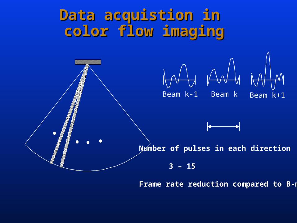
Data acquistion in Data acquistion in color flow imagingcolor flow imaging

Beam k-1 Beam k Beam k+1

Number of pulses in each direction

3 – 15

Frame rate reduction compared to B-mode

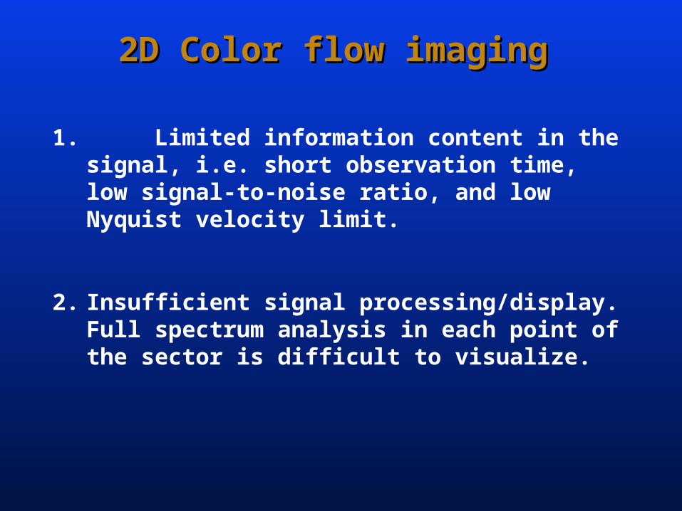
2D Color flow imaging2D Color flow imaging

1. Limited information content in the signal, i.e. short observation time, low signal-to-noise ratio, and low Nyquist velocity limit.

 

2. Insufficient signal processing/display. Full spectrum analysis in each point of the sector is difficult to visualize.

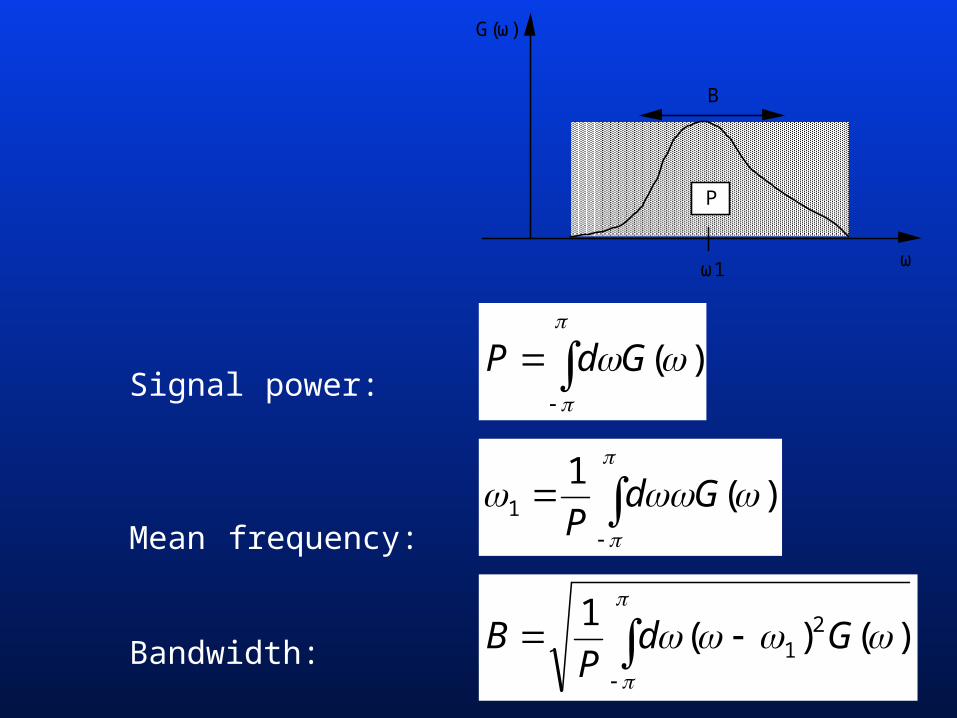
Signal power:  

Mean frequency:  

Bandwidth:

)(GdP

)(1

1 GdP

)()(1 2

1 GdP

B

G(ω)

P

B

ω1 ω

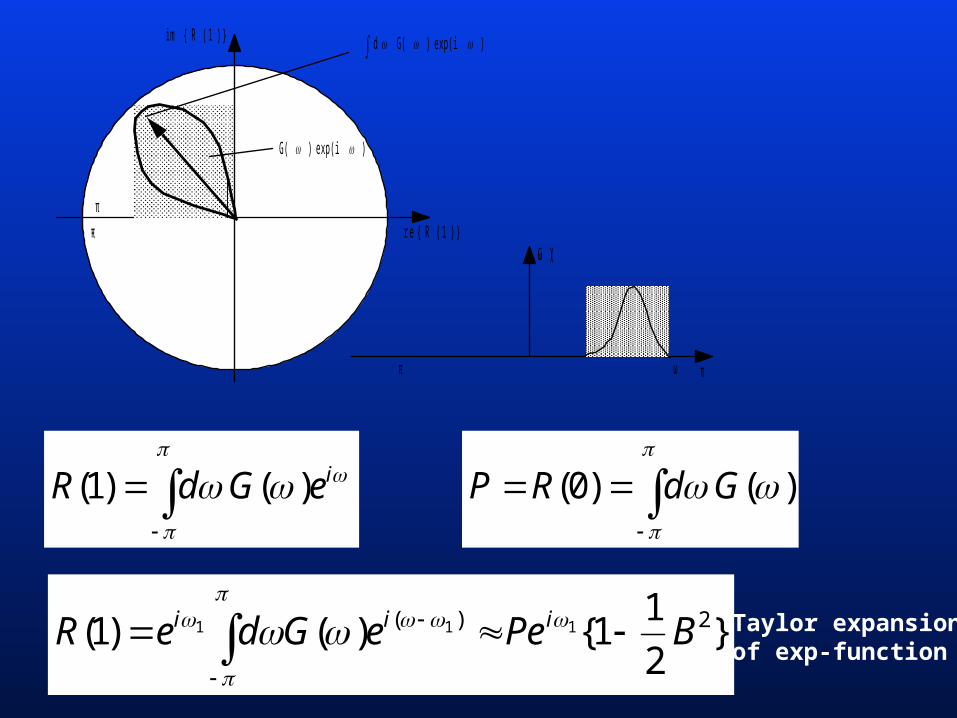
ieGdR )()1(

}2

11{ )()1( 2)( 111 BPeeGdeR iii

)exp(i )G(

)exp(i )G( d i m { R ( 1 ) }

r e { R ( 1 ) }

π

- πG (ω )

πω- π

Taylor expansionof exp-function

)()0( GdRP

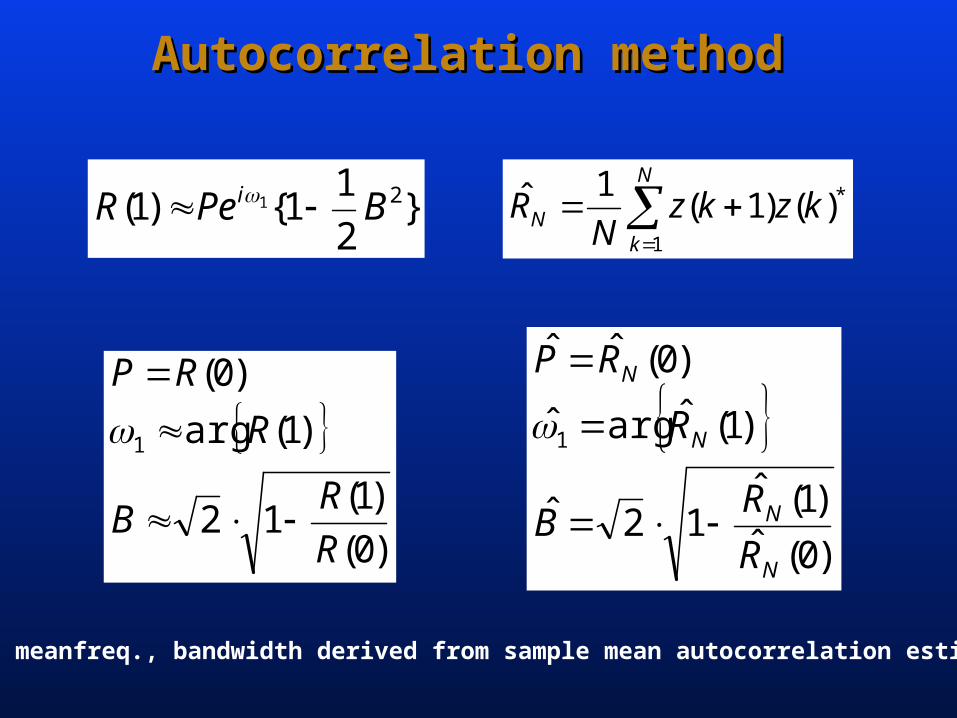
Autocorrelation methodAutocorrelation method

}2

11{ )1( 21 BPeR i

)0(

)1(12

)1(arg

)0(

1

R

RB

R

RP

N

kN kzkz

NR

1

*)()1(1ˆ

)0(ˆ)1(ˆ

12ˆ

)1(ˆargˆ

)0(ˆˆ

1

N

N

N

N

R

RB

R

RP

Power, meanfreq., bandwidth derived from sample mean autocorrelation estimator

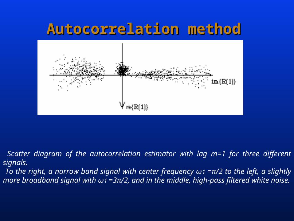
 Scatter diagram of the autocorrelation estimator with lag m=1 for three different signals. To the right, a narrow band signal with center frequency ω1 =π/2 to the left, a slightly more broadband signal with ω1 =3π/2, and in the middle, high-pass filtered white noise.

Autocorrelation methodAutocorrelation method

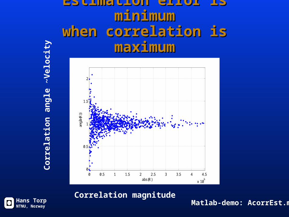
Estimation error is minimumEstimation error is minimumwhen correlation is maximumwhen correlation is maximum

Hans TorpNTNU, Norway

0 0.5 1 1.5 2 2.5 3 3.5 4 4.5

x 106

0

0.5

1

1.5

2

abs(R)

angl

e(R

))

Correlation magnitude

Cor

rela

tion

an

gle

~Vel

ocit

y

Matlab-demo: AcorrEst.m

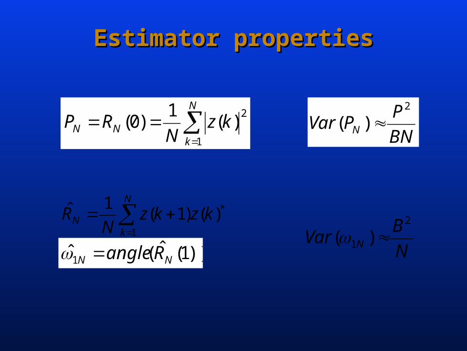
Estimator propertiesEstimator properties

BN

PPVar N

2

)(

N

kNN kz

NRP

1

2)(

1)0(

N

BVar N

2

1 )(

N

kN kzkz

NR

1

*)()1(1ˆ

))1(ˆ(ˆ1 NN Rangle

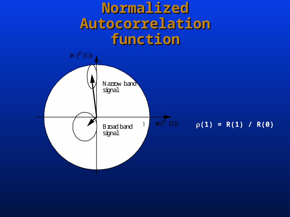
Normalized Autocorrelation Normalized Autocorrelation functionfunction

im{(1)}

re{ (1)}

Narrow band signal

Broad band signal

1

i

(1) = R(1) / R(0)

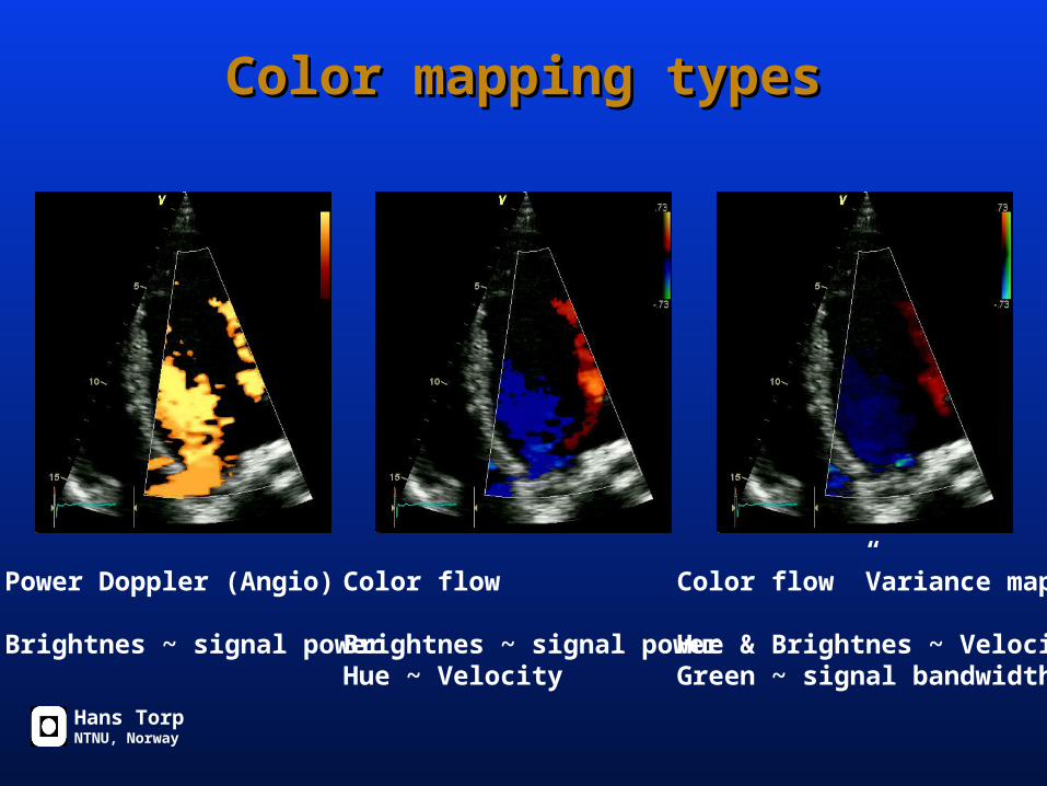
Color mapping typesColor mapping types

Hans TorpNTNU, Norway

Power Doppler (Angio)

Brightnes ~ signal power

Color flow

Brightnes ~ signal powerHue ~ Velocity

Color flow ”Variance map”

Hue & Brightnes ~ VelocityGreen ~ signal bandwidth

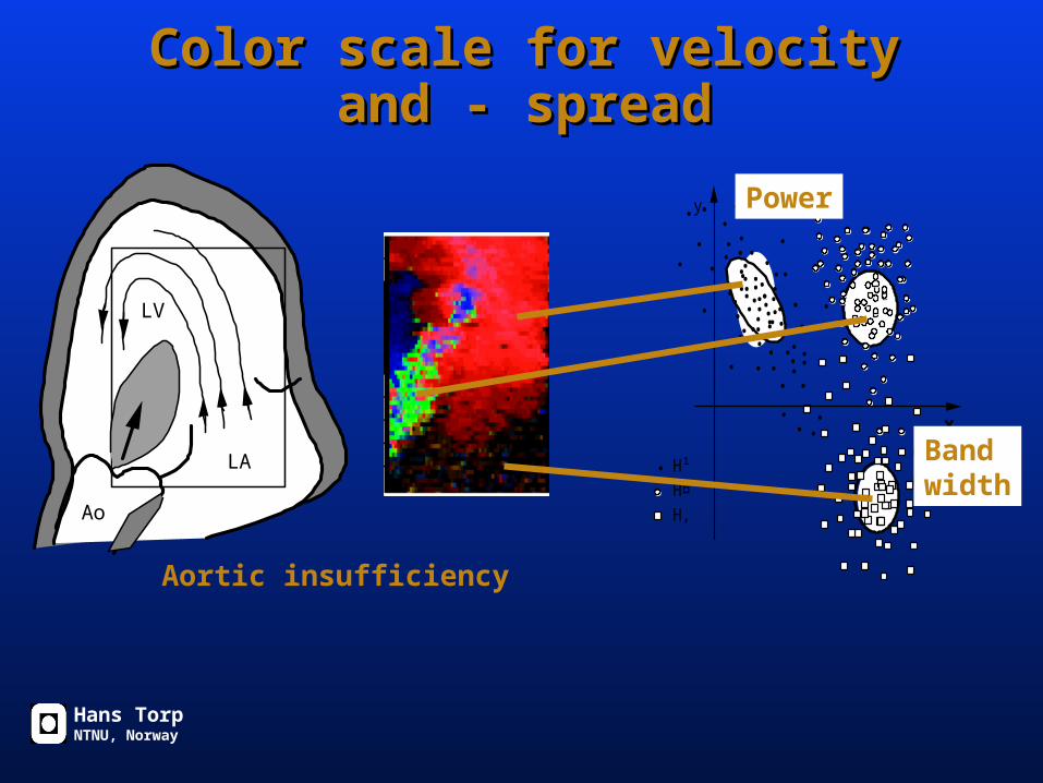
Color scale for velocity and - spreadColor scale for velocity and - spread

•• •

••

••

••

•• •• • •

••••

••

•

•••

••

••

•••

•

•

•

• • ••

•

•

•

•

•••

••••

••

•••• •

••

••••

••

•••

•••

•

• H¹H¤H‚

•

•

•

y

x

Ao

LV

LA

Power

Bandwidth

Aortic insufficiency

Hans TorpNTNU, Norway

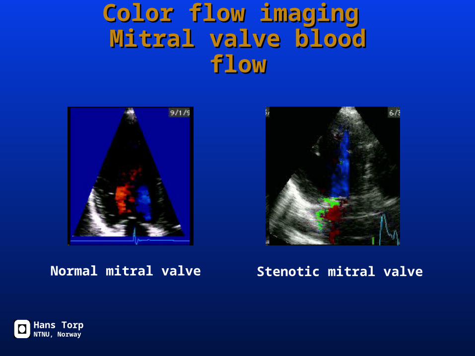
Color flow imaging Color flow imaging Mitral valve blood flowMitral valve blood flow

Normal mitral valve Stenotic mitral valve

Hans TorpNTNU, Norway

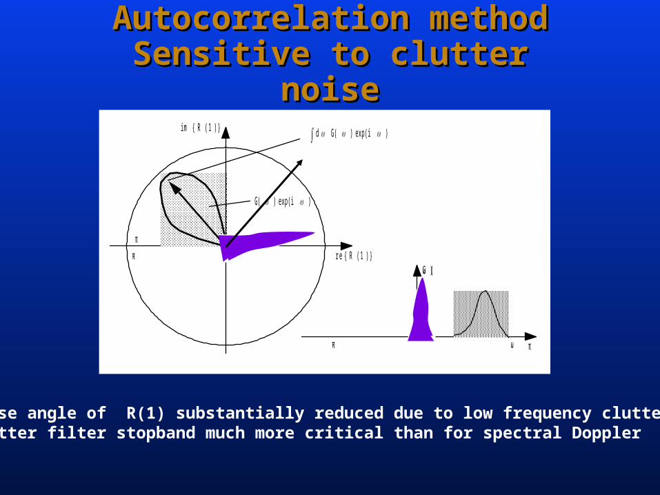
Autocorrelation methodAutocorrelation methodSensitive to clutter noiseSensitive to clutter noise

)exp(i )G(

)exp(i )G( d i m { R ( 1 ) }

r e { R ( 1 ) }

π

- πG (ω )

πω- π

Phase angle of R(1) substantially reduced due to low frequency clutter signalClutter filter stopband much more critical than for spectral Doppler

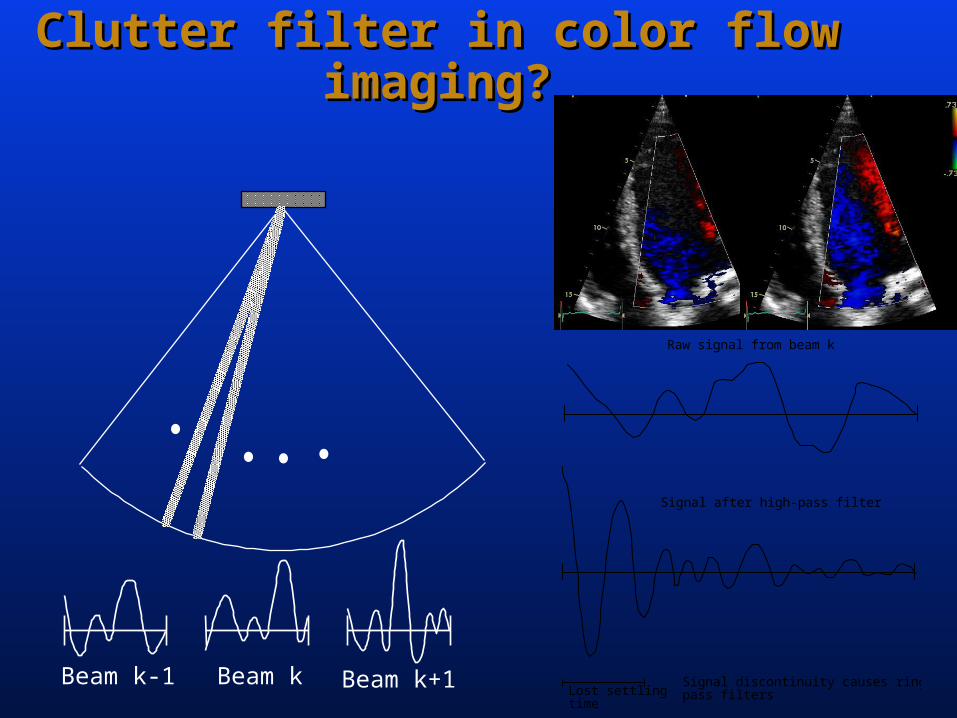
Clutter filter in color flow imaging?Clutter filter in color flow imaging?

Beam k-1 Beam k Beam k+1 Signal discontinuity causes ringing in high-pass filters

Raw signal from beam k

Signal after high-pass filter

Lost settling time

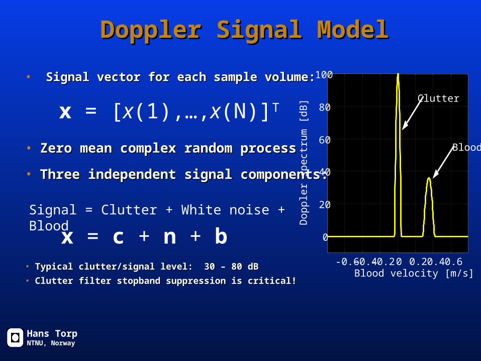
Doppler Signal ModelDoppler Signal Model

• Signal vector for each sample volume:Signal vector for each sample volume:

x = [x(1),…,x(N)]T

Signal = Clutter + White noise + Blood

x = c + n + b• Typical clutter/signal level: 30 – 80 dBTypical clutter/signal level: 30 – 80 dB

• Clutter filter stopband suppression is critical!Clutter filter stopband suppression is critical!

• Zero mean complex random processZero mean complex random process

• Three independent signal components:Three independent signal components:

Hans TorpNTNU, Norway

-0.6-0.4-0.2 0 0.2 0.4 0.6

0

20

40

60

80

100

Blood velocity [m/s]

Do

pp

ler

spe

ctru

m [

dB

]

Clutter

Blood

Approaches to clutter filteringApproaches to clutter filteringin color flow imagingin color flow imaging

• IIR-filter with initialization techniquesIIR-filter with initialization techniques

• Short FIR filtersShort FIR filters

• Regression filtersRegression filters

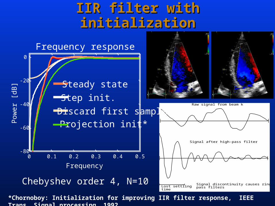
IIR filter with initializationIIR filter with initialization

Signal discontinuity causes ringing in high-pass filters

Raw signal from beam k

Signal after high-pass filter

Lost settling time

Chebyshev order 4, N=10

Pow

er [

dB]

Frequency

0 0.1 0.2 0.3 0.4 0.5-80

-60

-40

-20

0

Frequency response

Steady state

Step init.

Discard first samples

Projection init*

*Chornoboy: Initialization for improving IIR filter response, IEEE Trans. Signal processing, 1992

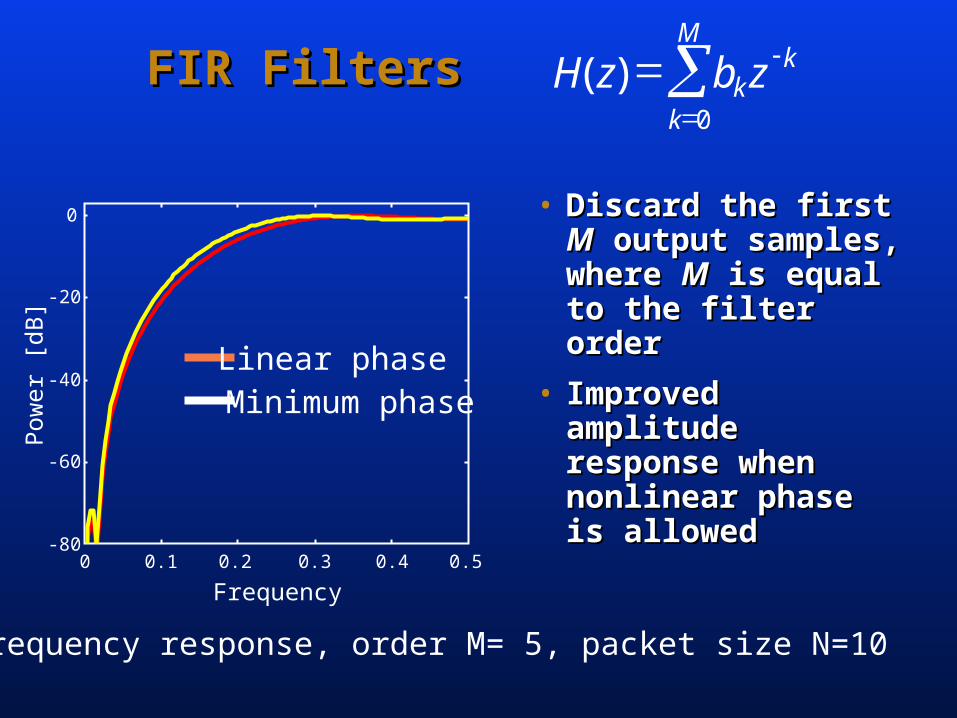
FIR FiltersFIR Filters

• Discard the first Discard the first MM output samples, where output samples, where MM is equal to the filter is equal to the filter orderorder

• Improved amplitude Improved amplitude response when nonlinear response when nonlinear phase is allowedphase is allowed

0 0.1 0.2 0.3 0.4 0.5-80

-60

-40

-20

0

Pow

er [

dB]

Frequency

Frequency response, order M= 5, packet size N=10

M

k

kkzbzH

0

)(

Linear phaseMinimum phase

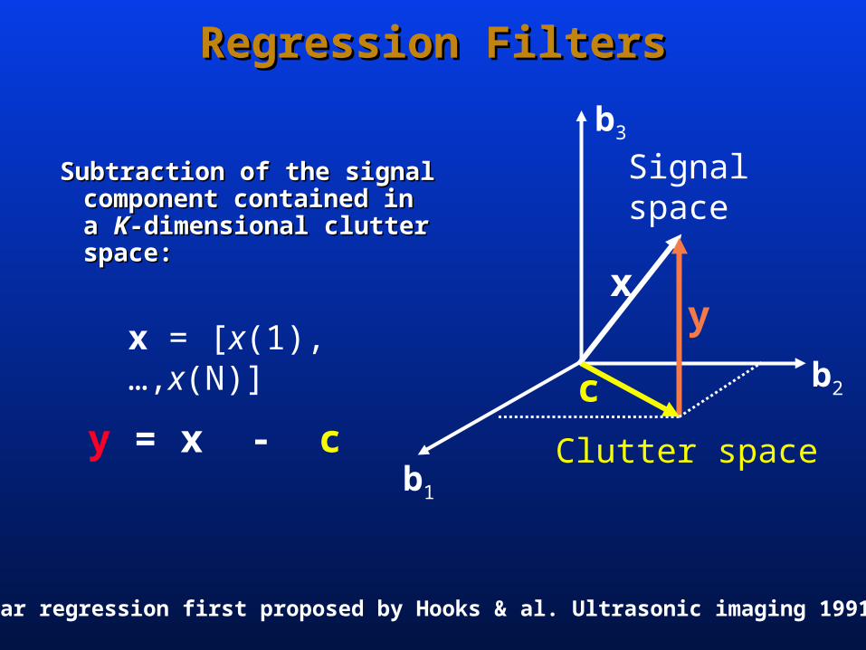
Regression FiltersRegression Filters

Subtraction of the signal Subtraction of the signal component contained in a component contained in a KK-dimensional clutter -dimensional clutter space:space:

Signal space

Clutter spaceb1

b2

b3

xy

cy = x - c

Linear regression first proposed by Hooks & al. Ultrasonic imaging 1991

x = [x(1),…,x(N)]

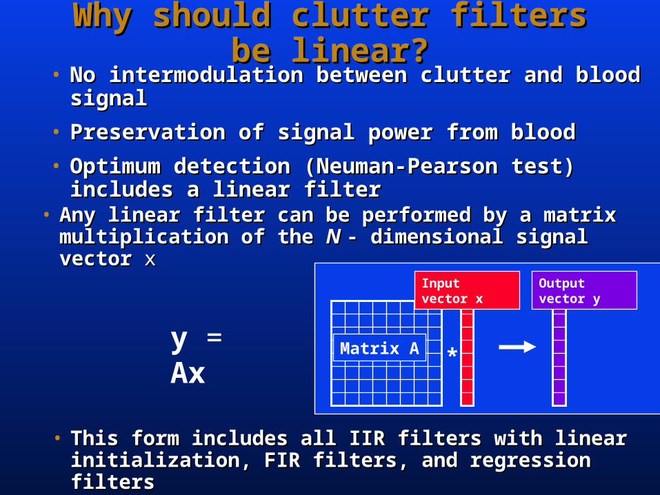
Why should clutter filters be linear?Why should clutter filters be linear?• No intermodulation between clutter and blood signalNo intermodulation between clutter and blood signal

• Preservation of signal power from bloodPreservation of signal power from blood

• Optimum detection (Neuman-Pearson test) includes a linear Optimum detection (Neuman-Pearson test) includes a linear filter filter

y = Ax

• Any linear filter can be performed by a matrix multiplication Any linear filter can be performed by a matrix multiplication of the of the N N - dimensional signal vector - dimensional signal vector xx

• This form includes all IIR filters with linear initialization, FIR This form includes all IIR filters with linear initialization, FIR filters, and regression filtersfilters, and regression filters

*Matrix A

Input vector x Output vector y

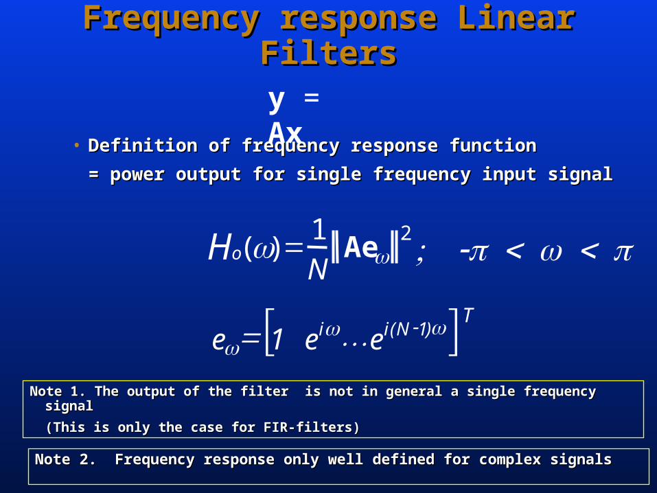
Frequency response Linear FiltersFrequency response Linear Filters

y = Ax

• Definition of frequency response function Definition of frequency response function

= power output for single frequency input signal= power output for single frequency input signal

21)( Ae

NHo

TNii eee

)1(1

Note 1. The output of the filter is not in general a single frequency signalNote 1. The output of the filter is not in general a single frequency signal

(This is only the case for FIR-filters)(This is only the case for FIR-filters)

Note 2. Frequency response only well defined for complex signalsNote 2. Frequency response only well defined for complex signals

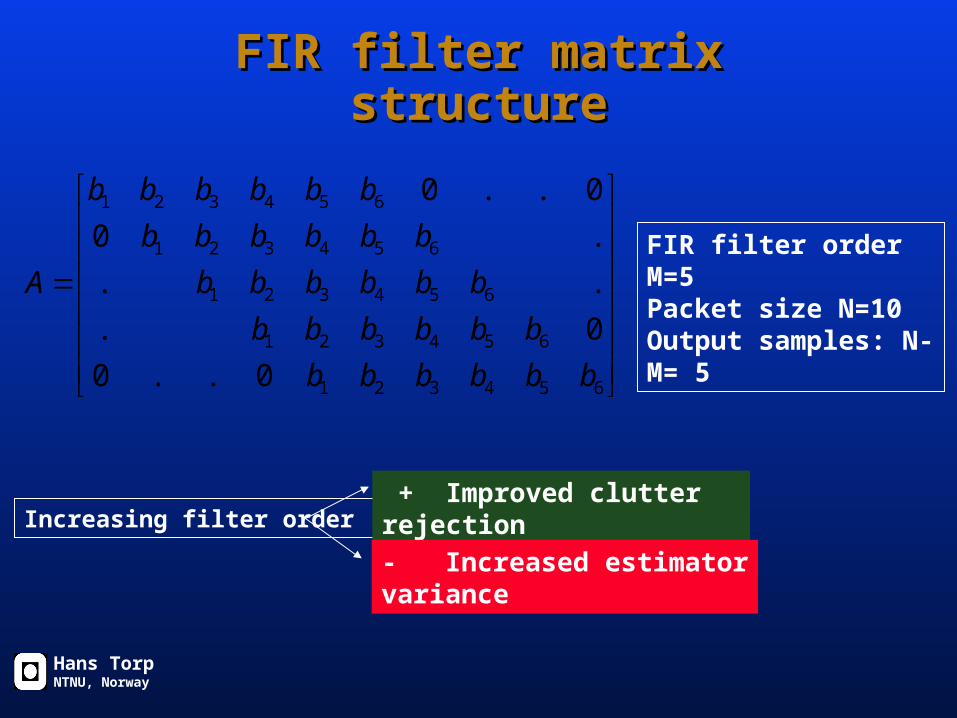
FIR filter matrix structureFIR filter matrix structure

654321

654321

654321

654321

654321

0..0

0.

..

.0

0..0

bbbbbb

bbbbbb

bbbbbb

bbbbbb

bbbbbb

AFIR filter order M=5Packet size N=10Output samples: N-M= 5

Increasing filter order + Improved clutter rejection

- Increased estimator variance

Hans TorpNTNU, Norway

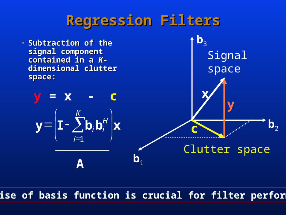
Regression FiltersRegression Filters

• Subtraction of the signal Subtraction of the signal component contained in a component contained in a KK-dimensional clutter -dimensional clutter space:space:

xbbIy

K

i

Hii

1

Signal space

Clutter spaceb1

b2

b3

xy

c

Choise of basis function is crucial for filter performance

y = x - c

A

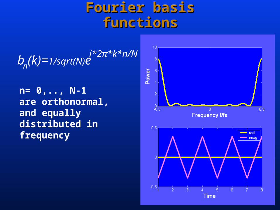
Fourier basis functionsFourier basis functions

nb (k)=1/sqrt(N)ei*2π*k*n/N

n= 0,.., N-1are orthonormal, and equally distributed in frequency

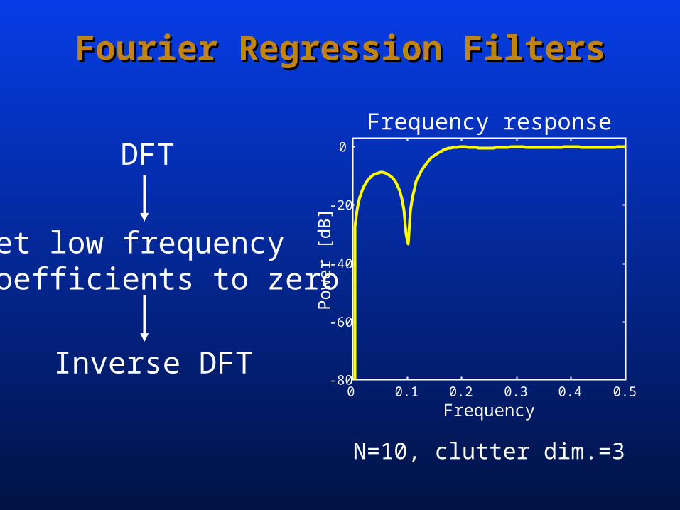
Fourier Regression FiltersFourier Regression Filters

DFT

Set low frequency coefficients to zero

Inverse DFT0 0.1 0.2 0.3 0.4 0.5

-80

-60

-40

-20

0

Frequency

Pow

er [

dB]

Frequency response

N=10, clutter dim.=3

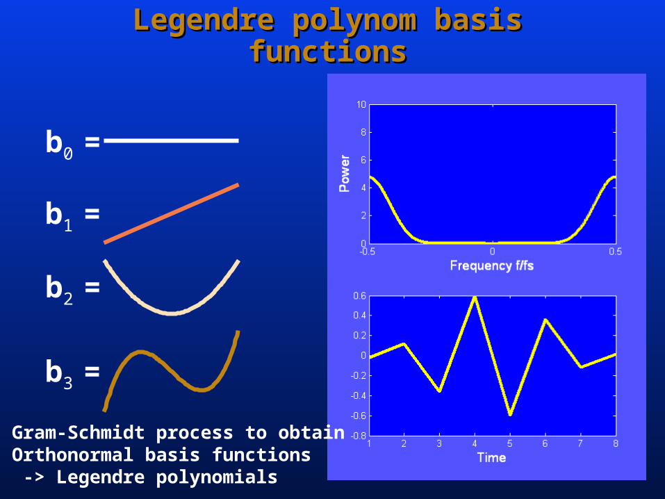
Legendre polynom basis functionsLegendre polynom basis functions

b0 =

b1 =

b2 =

b3 =

Gram-Schmidt process to obtainOrthonormal basis functions -> Legendre polynomials

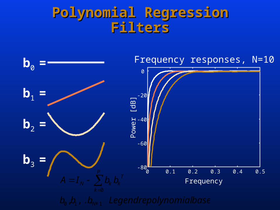
Polynomial Regression FiltersPolynomial Regression Filters

b0 =

b1 =

b2 =

b3 =

Pow

er [

dB]

Frequency

0 0.1 0.2 0.3 0.4 0.5-80

-60

-40

-20

0

Frequency responses, N=10

basepolynomialLegendrebbb

bbIA

N

P

k

TkkN

110

0

,..,,

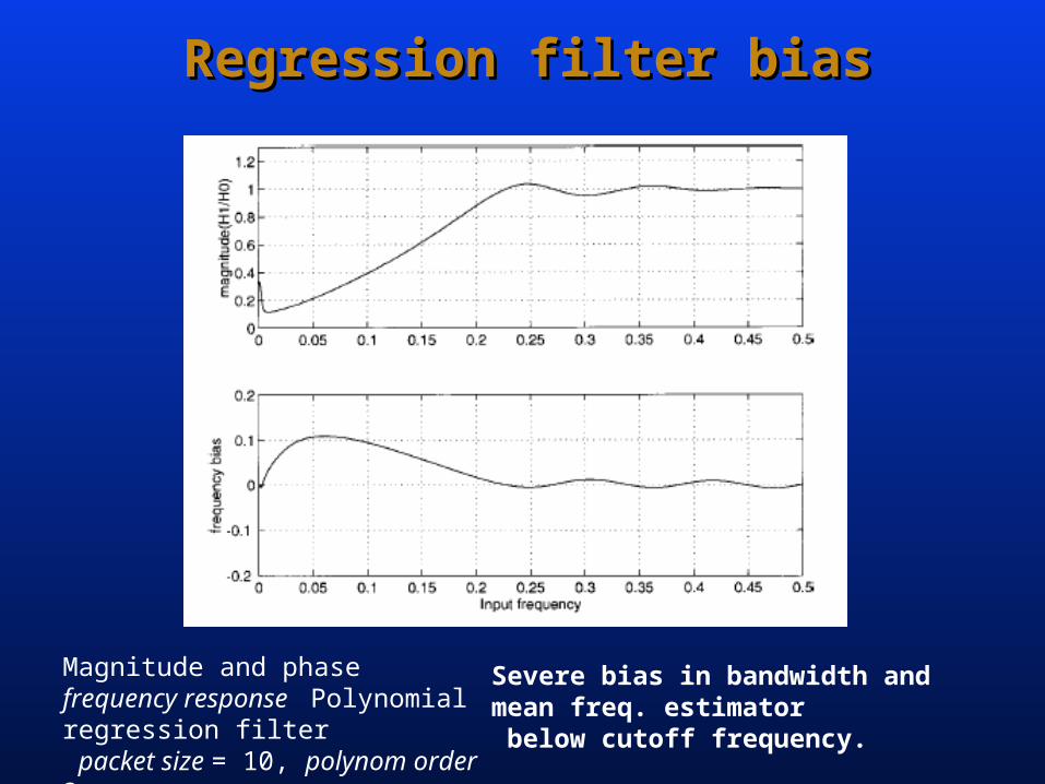
Regression filter biasRegression filter bias

Magnitude and phase frequency response Polynomial regression filter packet size = 10, polynom order 3.

Severe bias in bandwidth and mean freq. estimator below cutoff frequency.

How to image low velocity flowHow to image low velocity flow

• Long observation time neededLong observation time needed

• Obtained by increased packet size or lower PRFObtained by increased packet size or lower PRF

• Beam interleaving permits lower prf without loss in Beam interleaving permits lower prf without loss in framerateframerate

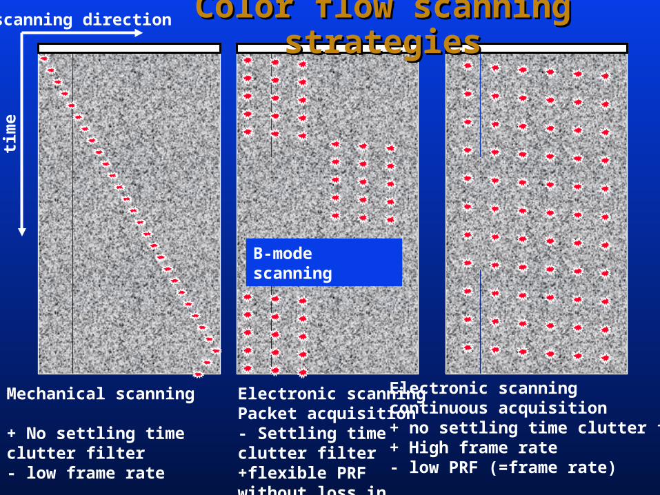
Color flow scanning strategiesColor flow scanning strategies

B-mode scanning

Mechanical scanning

+ No settling time clutter filter- low frame rate

Electronic scanning Packet acquisition- Settling time clutter filter+flexible PRF without loss in frame rate

Electronic scanning continuous acquisition+ no settling time clutter filter+ High frame rate- low PRF (=frame rate)

scanning directionti

me

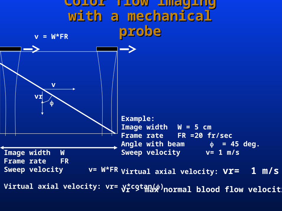
Color flow imaging with a Color flow imaging with a mechanical probemechanical probe

v = W*FR

Image width WFrame rate FRSweep velocity v= W*FR

Virtual axial velocity: vr= v*cotan()

vr

v

Example:Image width W = 5 cmFrame rate FR =20 fr/secAngle with beam = 45 deg.Sweep velocity v= 1 m/s

Virtual axial velocity: vr= 1 m/s

vr > max normal blood flow velocities!

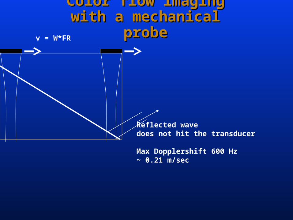
Color flow imaging with a Color flow imaging with a mechanical probemechanical probe

v = W*FR

Reflected wavedoes not hit the transducer

Max Dopplershift 600 Hz~ 0.21 m/sec

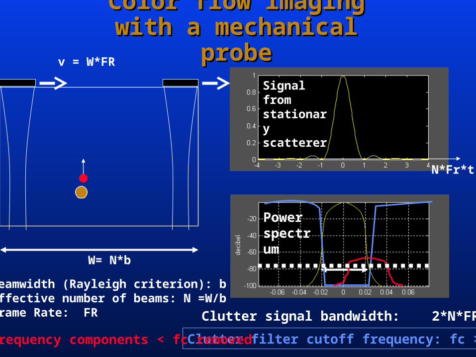
Color flow imaging with a Color flow imaging with a mechanical probemechanical probe

W= N*b

v = W*FR

Beamwidth (Rayleigh criterion): bEffective number of beams: N =W/bFrame Rate: FR

Signal from stationary scatterer

N*Fr*t

Clutter signal bandwidth: 2*N*FR

Power spectrum

Clutter filter cutoff frequency: fc > N*FR Frequency components < fc removed

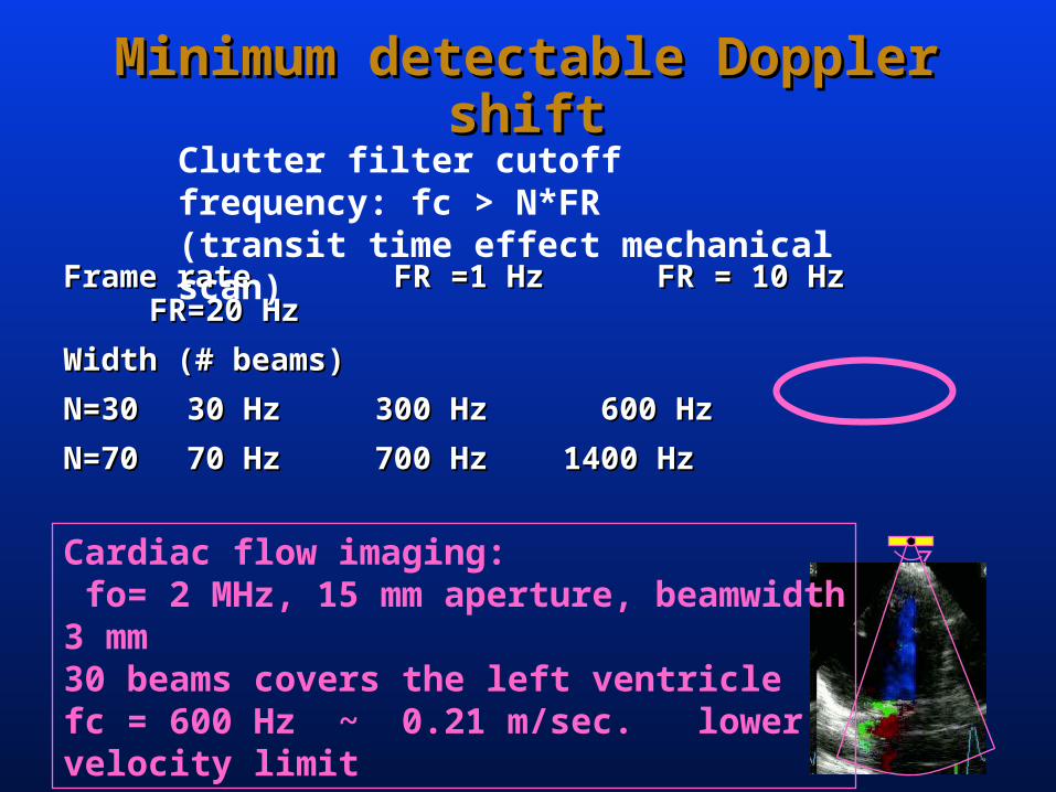
Minimum detectable Doppler shiftMinimum detectable Doppler shift

Frame rate Frame rate FR =1 Hz FR =1 Hz FR = 10 Hz FR=20 Hz FR = 10 Hz FR=20 Hz

Width (# beams)Width (# beams)

N=30N=30 30 Hz30 Hz 300 Hz300 Hz 600 Hz 600 Hz

N=70N=70 70 Hz70 Hz 700 Hz700 Hz 1400 Hz1400 Hz

Clutter filter cutoff frequency: fc > N*FR(transit time effect mechanical scan)

Cardiac flow imaging: fo= 2 MHz, 15 mm aperture, beamwidth 3 mm30 beams covers the left ventriclefc = 600 Hz ~ 0.21 m/sec. lower velocity limit

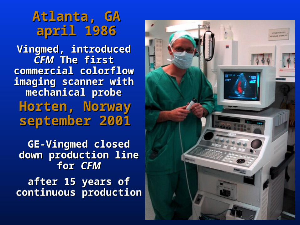
Atlanta, GA april 1986Atlanta, GA april 1986

Vingmed, introduced Vingmed, introduced CFMCFM The first commercial The first commercial

colorflow imaging scanner colorflow imaging scanner with mechanical probewith mechanical probe

Horten, Norway Horten, Norway september 2001september 2001

GE-Vingmed closed down GE-Vingmed closed down production line for production line for CFMCFM

after 15 years of continuous after 15 years of continuous productionproduction

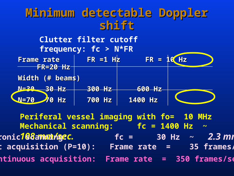
Minimum detectable Doppler shiftMinimum detectable Doppler shift

Clutter filter cutoff frequency: fc > N*FR

Frame rate Frame rate FR =1 Hz FR =1 Hz FR = 10 Hz FR = 10 Hz FR=20 Hz FR=20 Hz

Width (# beams)Width (# beams)

N=30N=30 30 Hz30 Hz 300 Hz300 Hz 600 Hz 600 Hz

N=70N=70 70 Hz70 Hz 700 Hz700 Hz 1400 Hz1400 Hz

Periferal vessel imaging with fo= 10 MHzMechanical scanning: fc = 1400 Hz ~ 108 mm/sec. Electronic scanning: fc = 30 Hz ~ 2.3 mm/sec.

Packet acquisition (P=10): Frame rate = 35 frames/sec

Continuous acquisition: Frame rate = 350 frames/sec

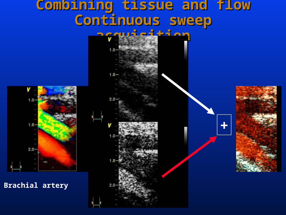
Combining tissue and flowCombining tissue and flowContinuous sweep acquisitionContinuous sweep acquisition

+

Brachial artery