Geoscience Laser Altimeter System (GLAS)

Algorithm Theoretical Basis DocumentVersion 2.2

PRECISION ATTITUDE DETERMINATION(PAD)

Prepared by

Sungkoo BaeBob E. Schutz

Center for Space ResearchThe University of Texas at Austin

October 2002

TABLEOF CONTENTS

GLOSSARY 2

1 INTRODUCTION 3

1.1 GLAS Measurement Requirement . . . . . . . . . . . . . . . . 31.2 GLAS Attitude/Pointing Requirement . . . . . . . . . . . . . 51.3 Outline of Document . . . . . . . . . . . . . . . . . . . . . . . 8

2 FUNDAMENTALS OF ATTITUDE DETERMINATION 10

2.1 Coordinate Systems . . . . . . . . . . . . . . . . . . . . . . . 102.2 Quaternion Representation . . . . . . . . . . . . . . . . . . . 112.3 Kinematic Equations of Spacecraft Attitude . . . . . . . . . . 142.4 Dynamical Equations of Spacecraft Attitude . . . . . . . . . . 152.5 Attitude Determination Problem . . . . . . . . . . . . . . . . 16

3 MEASUREMENT SYSTEM 18

3.1 CCD Star Tracker . . . . . . . . . . . . . . . . . . . . . . . . 183.2 Hemispherical Resonator Gyro . . . . . . . . . . . . . . . . . 263.3 Star Catalog . . . . . . . . . . . . . . . . . . . . . . . . . . . 29

4 STAR IDENTIFICATION 33

4.1 Pattern Matching Algorithm . . . . . . . . . . . . . . . . . . 344.2 Direct Match Technique . . . . . . . . . . . . . . . . . . . . . 42

5 ATTITUDE DETERMINATION 49

5.1 Single Frame Attitude Determination . . . . . . . . . . . . . . 495.2 Extended Kalman Filter . . . . . . . . . . . . . . . . . . . . . 545.3 Batch Method . . . . . . . . . . . . . . . . . . . . . . . . . . . 585.4 Simulation Results . . . . . . . . . . . . . . . . . . . . . . . . 59

6 POINTING DETERMINATION 67

6.1 Pointing Determination Algorithm . . . . . . . . . . . . . . . 676.2 Spacecraft Velocity In uence on Laser Pointing . . . . . . . . 766.3 Systematic Errors . . . . . . . . . . . . . . . . . . . . . . . . . 78

7 IMPLEMENTATION CONSIDERATIONS 82

7.1 Standards . . . . . . . . . . . . . . . . . . . . . . . . . . . . . 827.2 Ancillary Inputs . . . . . . . . . . . . . . . . . . . . . . . . . 837.3 Accuracy and Validation . . . . . . . . . . . . . . . . . . . . . 837.4 Computational: CPU, Memory and Disk Storage . . . . . . . 847.5 Sensor Failures . . . . . . . . . . . . . . . . . . . . . . . . . . 84

BIBLIOGRAPHY 86

ACKNOWLEDGMENTS 90

Appendix.A PROPERTIES OF QUATERNIONS 91

1

GLOSSARY

ATBD Algorithm Theoretical Basis DocumentBD Boresight DirectionCCD Charge Coupled DeviceCRF Celestial Reference FrameCRS Collimated Reference SourceDMT Direct Match TechniqueEKF Extended Kalman FilterFOAM Fast Optimal Attitude MethodFOV Field of ViewGCF Gyro Coordinate FrameHP Hewlett PackardHRG Hemispherical Resonator GyroICRF International Celestial Reference FrameIERS International Earth Rotation ServiceIPD Improved Polar DecompositionITER Iteration MethodITRF International Terrestrial Reference FrameLPA Laser Pro�ling ArrayLRC Laser Reference CameraLRS Laser Reference SensorLRT Laser Reference TelescopeLTR Lateral Transfer Retrore ectorMFOAM Modi�ed Fast Optimal Attitude MethodMSX Midcourse Space ExperimentOBF Optical Bench Coordinate FramePAD Precision Attitude DeterminationPD Polar DecompositionPMA Pattern Matching AlgorithmPOD Precision Orbit DeterminationQUEST Quaternion EstimatorSCF Star Tracker Coordinate FrameSFAD Single Frame Attitude DeterminationSRS Stellar Reference SystemSVD Singular Value DecompositionTRF Terrestrial Reference FrameUVF Unit Vector Filter

2

Chapter 1

INTRODUCTION

The Geoscience Laser Altimeter System (GLAS) instrument is planned to be launched onthe Ice, Cloud and land Elevation Satellite (ICESAT) in December 2002 as a part of theEarth Observing System (EOS) of NASA. The primary purpose of the GLAS mission is tomake ice sheet elevation measurements in the polar regions which will be used to determinethe mass balance of the ice sheets and their contributions to global sea level change [31].In addition, the measurements will meet science objectives to support atmospheric science,and land topography application. The laser altimeter will measure the height from thespacecraft to Greenland and Antarctic ice sheets to support investigations of the secularchange in surface elevation, as well as annual, interannual, and other temporal variations.To support the science requirements to determine temporal elevation change, the mea-surements by the GLAS instrumentation must be very accurate. The ICESAT orbit willbe near-circular (eccentricity = 0.0013), with a semimajor axis of 6970 km, and it will benear polar, with an inclination of 94�, in order to y over Greenland and Antarctica. Theorbit is frozen so that the mean perigee is �xed near the north pole. The GLAS/ICESAThas a 3 year lifetime requirement with a 5 year goal. The EOS program plans for follow-onsatellites to extend the science data set to 15 years and longer.

1.1 GLAS Measurement Requirement

The GLAS Science Requirements [47] provide the error budget for the instrument andancillary information necessary to meet the science requirements. The most stringentrequirements are needed for the cryosphere objectives. For example, the accuracy ofelevation change in the vicinity of the West Antarctic Ross ice streams is 1.5 cm/yr in a100 � 100 km2 area where surface slopes are < 0:6�. In summary, the error budget allows10 cm instrument precision, 5 cm radial orbit position, 7.5 cm laser pointing knowledge and2 cm or less for other error contributors. The GLAS orbit position will be obtained withthe Global Positioning System (GPS) and ground-based Satellite Laser Ranging (SLR).In addition to the geocentric position vector, the accurate determination of the altimeterbeam pointing angle in an Earth-�xed Terrestrial Reference Frame (TRF) is also requiredfor high-precision satellite laser altimetry. The laser altimeter will provide the range

3

GLAS @ 600 km

EEEEEEEEEEEEEEEEEEEEEEEEEEE

- �(1 arcsec)(600 km) � 2.9 m

- �

1 arcsec

PPPPPPPPPPPP1�Slope InducedRange Error

?

6

(2.9 m) tan 1� � 5.1 cm(2.9 m) tan 2� � 10.1 cm(2.9 m) tan 3� � 15.2 cm

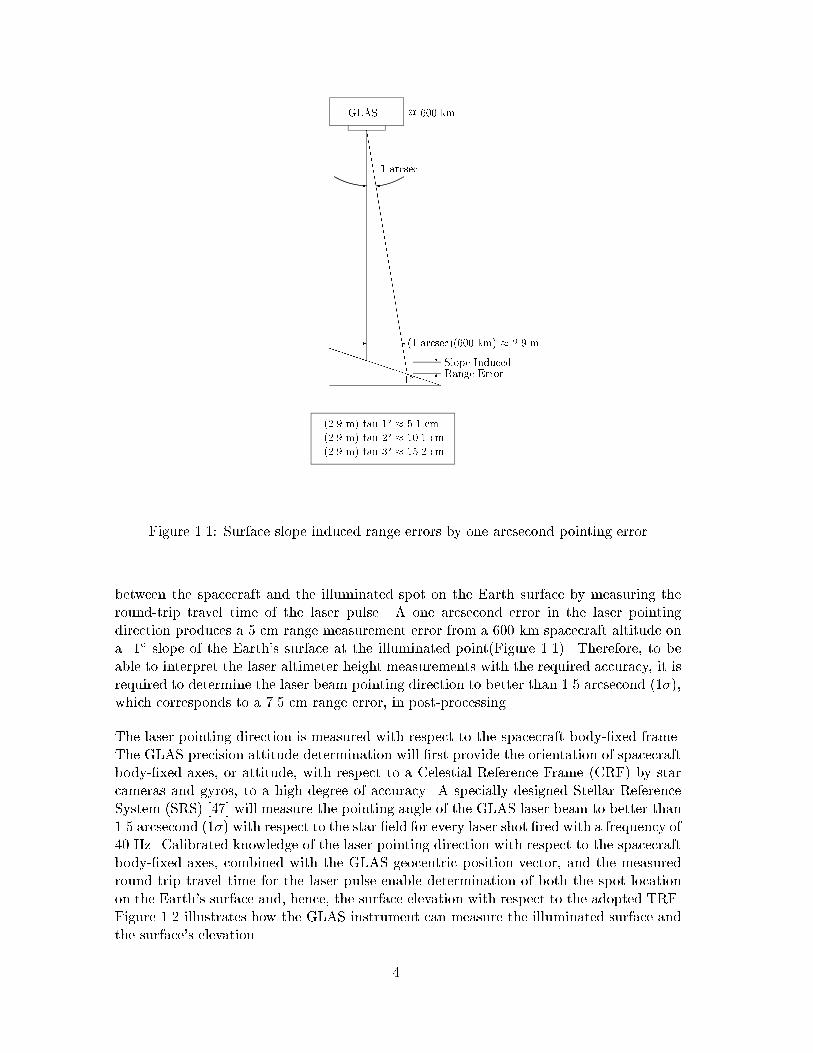
Figure 1.1: Surface slope induced range errors by one arcsecond pointing error

between the spacecraft and the illuminated spot on the Earth surface by measuring theround-trip travel time of the laser pulse. A one arcsecond error in the laser pointingdirection produces a 5 cm range measurement error from a 600 km spacecraft altitude ona 1� slope of the Earth's surface at the illuminated point(Figure 1.1). Therefore, to beable to interpret the laser altimeter height measurements with the required accuracy, it isrequired to determine the laser beam pointing direction to better than 1.5 arcsecond (1�),which corresponds to a 7.5 cm range error, in post-processing.

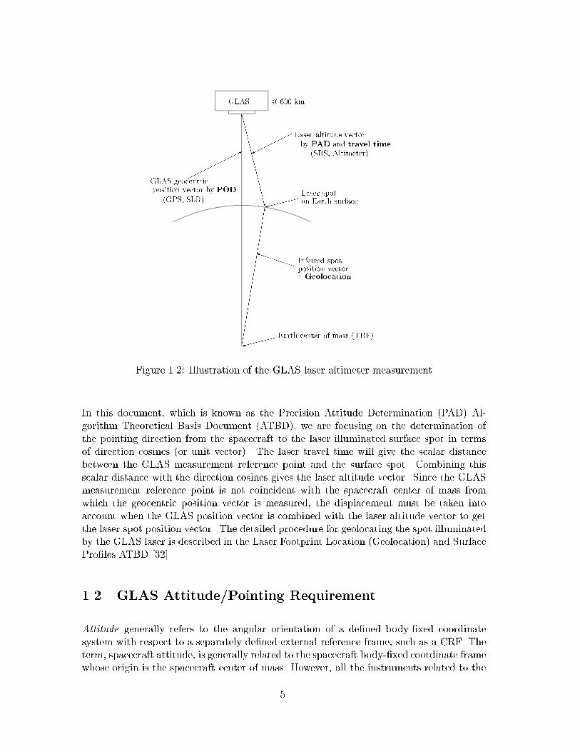
The laser pointing direction is measured with respect to the spacecraft body-�xed frame.The GLAS precision attitude determination will �rst provide the orientation of spacecraftbody-�xed axes, or attitude, with respect to a Celestial Reference Frame (CRF) by starcameras and gyros, to a high degree of accuracy. A specially designed Stellar ReferenceSystem (SRS) [47] will measure the pointing angle of the GLAS laser beam to better than1.5 arcsecond (1�) with respect to the star �eld for every laser shot �red with a frequency of40 Hz. Calibrated knowledge of the laser pointing direction with respect to the spacecraftbody-�xed axes, combined with the GLAS geocentric position vector, and the measuredround trip travel time for the laser pulse enable determination of both the spot locationon the Earth's surface and, hence, the surface elevation with respect to the adopted TRF.Figure 1.2 illustrates how the GLAS instrument can measure the illuminated surface andthe surface's elevation.

4

GLAS @ 600 km

6CCCCCCCCCCCCCCW

�����������������������

����

����*

GLAS geocentricposition vector by POD

(GPS, SLR)

�������

Laser altitude vectorby PAD and travel time

(SRS, Altimeter)

�����9

Laser spoton Earth surface

PPPP

PPiInferred spotposition vector: Geolocation

�����9Earth center of mass (TRF)

Figure 1.2: Illustration of the GLAS laser altimeter measurement

In this document, which is known as the Precision Attitude Determination (PAD) Al-gorithm Theoretical Basis Document (ATBD), we are focusing on the determination ofthe pointing direction from the spacecraft to the laser illuminated surface spot in termsof direction cosines (or unit vector). The laser travel time will give the scalar distancebetween the GLAS measurement reference point and the surface spot. Combining thisscalar distance with the direction cosines gives the laser altitude vector. Since the GLASmeasurement reference point is not coincident with the spacecraft center of mass fromwhich the geocentric position vector is measured, the displacement must be taken intoaccount when the GLAS position vector is combined with the laser altitude vector to getthe laser spot position vector. The detailed procedure for geolocating the spot illuminatedby the GLAS laser is described in the Laser Footprint Location (Geolocation) and SurfacePro�les ATBD [32].

1.2 GLAS Attitude/Pointing Requirement

Attitude generally refers to the angular orientation of a de�ned body-�xed coordinatesystem with respect to a separately de�ned external reference frame, such as a CRF. Theterm, spacecraft attitude, is generally related to the spacecraft body-�xed coordinate framewhose origin is the spacecraft center of mass. However, all the instruments related to the

5

PAD will be attatched to the GLAS optical bench. Consequently, the more convenientchoice for the origin of the body-�xed coordinate frame is an instrument reference pointpositioned at the optical bench and the corresponing coordinate frame will de�ne theoptical bench attitude as a replacement of the common spacecraft attitude. Thoughoutthis document, we are basically concerned with the optical bench attitude for the GLAS,rather than the spacecraft attitude. Spacecraft attitude is sometimes mentioned, but itis an alternative terminology for the optical bench attitude when we discuss the GLASPAD. Attitude determination refers to the process of determining the angular orientationof the spacecraft-�xed axes or optical bench axes from measurements obtained by variousattitude sensors. This determination of attitude uses data from appropriate sensors and asophisticated processing of the sensor data.

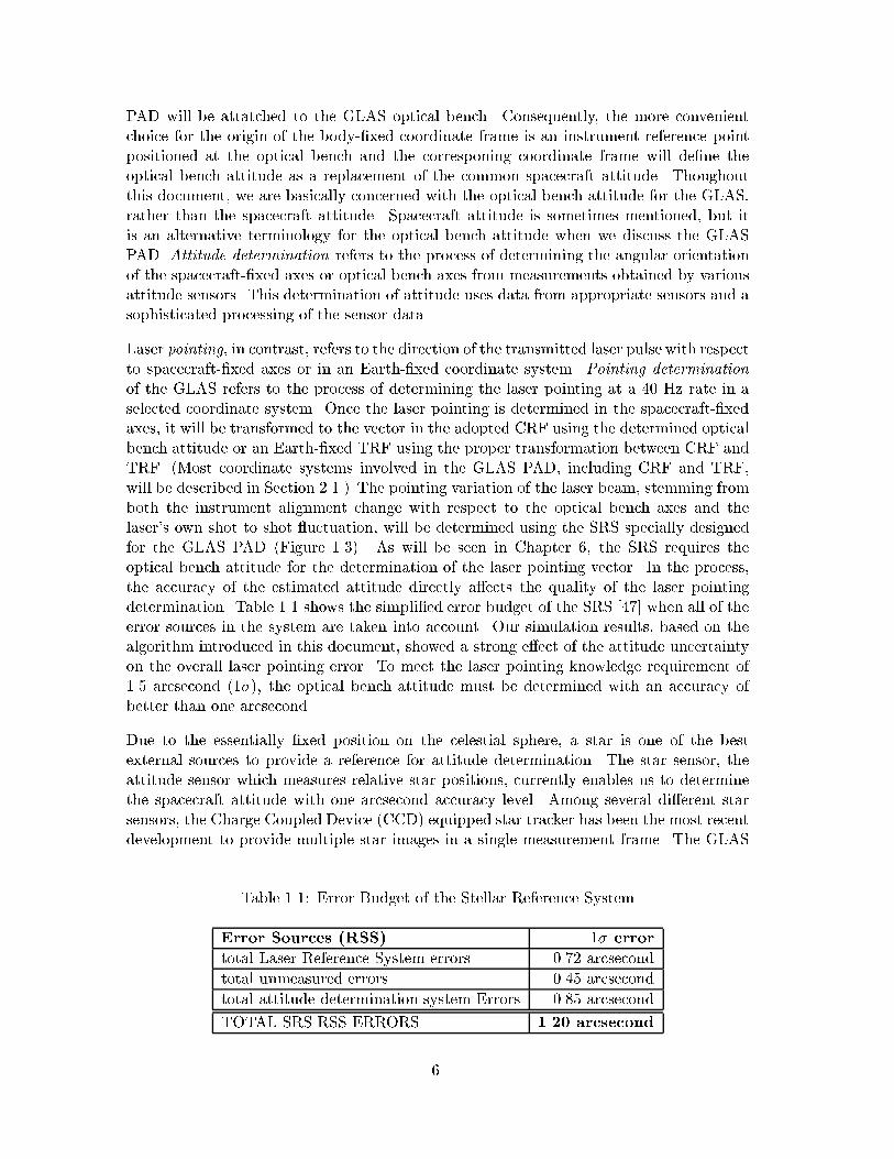
Laser pointing, in contrast, refers to the direction of the transmitted laser pulse with respectto spacecraft-�xed axes or in an Earth-�xed coordinate system. Pointing determinationof the GLAS refers to the process of determining the laser pointing at a 40 Hz rate in aselected coordinate system. Once the laser pointing is determined in the spacecraft-�xedaxes, it will be transformed to the vector in the adopted CRF using the determined opticalbench attitude or an Earth-�xed TRF using the proper transformation between CRF andTRF. (Most coordinate systems involved in the GLAS PAD, including CRF and TRF,will be described in Section 2.1.) The pointing variation of the laser beam, stemming fromboth the instrument alignment change with respect to the optical bench axes and thelaser's own shot to shot uctuation, will be determined using the SRS specially designedfor the GLAS PAD (Figure 1.3). As will be seen in Chapter 6, the SRS requires theoptical bench attitude for the determination of the laser pointing vector. In the process,the accuracy of the estimated attitude directly a�ects the quality of the laser pointingdetermination. Table 1.1 shows the simpli�ed error budget of the SRS [47] when all of theerror sources in the system are taken into account. Our simulation results, based on thealgorithm introduced in this document, showed a strong e�ect of the attitude uncertaintyon the overall laser pointing error. To meet the laser pointing knowledge requirement of1.5 arcsecond (1�), the optical bench attitude must be determined with an accuracy ofbetter than one arcsecond.

Due to the essentially �xed position on the celestial sphere, a star is one of the bestexternal sources to provide a reference for attitude determination. The star sensor, theattitude sensor which measures relative star positions, currently enables us to determinethe spacecraft attitude with one arcsecond accuracy level. Among several di�erent starsensors, the Charge Coupled Device (CCD) equipped star tracker has been the most recentdevelopment to provide multiple star images in a single measurement frame. The GLAS

Table 1.1: Error Budget of the Stellar Reference System

Error Sources (RSS) 1� error

total Laser Reference System errors 0.72 arcsecond

total unmeasured errors 0.45 arcsecond

total attitude determination system Errors 0.85 arcsecond

TOTAL SRS RSS ERRORS 1.20 arcsecond

6

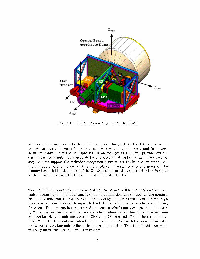
Figure 1.3: Stellar Reference System on the GLAS

attitude system includes a Raytheon Optical System Inc.(ROSI) HD-1003 star tracker asthe primary attitude sensor in order to achieve the required one arcsecond (or better)accuracy. Additionally, the Hemispherical Resonator Gyros (HRG) will provide continu-ously measured angular rates associated with spacecraft attitude changes. The measuredangular rates support the attitude propagation between star tracker measurements andthe attitude prediction when no stars are available. The star tracker and gyros will bemounted on a rigid optical bench of the GLAS instrument; thus, this tracker is referred toas the optical bench star tracker or the instrument star tracker.

Two Ball CT-602 star trackers, products of Ball Aerospace, will be mounted on the space-craft structure to support real time attitude determination and control. In the nominal600 km altitude orbit, the GLAS Attitude Control System (ACS) must continually changethe spacecraft orientation with respect to the CRF to maintain a near-nadir laser pointingdirection. Thus, magnetic torquers and momentum wheels must change the orientationby 223 arcsec/sec with respect to the stars, which de�ne inertial directions. The real timeattitude knowledge requirement of the ICESAT is 20 arcseconds (1�) or better. The BallCT-602 star trackers' data are intended to be used in the PAD with the optical bench startracker or as a backup unit to the optical bench star tracker. The study in this documentwill only utilize the optical bench star tracker.

7

1.3 Outline of Document

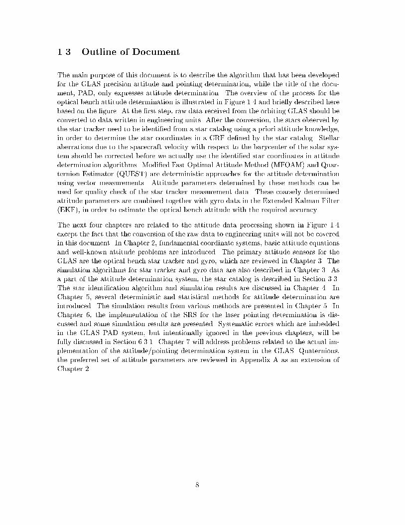
The main purpose of this document is to describe the algorithm that has been developedfor the GLAS precision attitude and pointing determination, while the title of the docu-ment, PAD, only expresses attitude determination. The overview of the process for theoptical bench attitude determination is illustrated in Figure 1.4 and brie y described herebased on the �gure. At the �rst step, raw data received from the orbiting GLAS should beconverted to data written in engineering units. After the conversion, the stars observed bythe star tracker need to be identi�ed from a star catalog using a priori attitude knowledge,in order to determine the star coordinates in a CRF de�ned by the star catalog. Stellaraberrations due to the spacecraft velocity with respect to the barycenter of the solar sys-tem should be corrected before we actually use the identi�ed star coordinates in attitudedetermination algorithms. Modi�ed Fast Optimal Attitude Method (MFOAM) and Quar-ternion Estimator (QUEST) are deterministic approaches for the attitude determinationusing vector measurements. Attitude parameters determined by these methods can beused for quality check of the star tracker measurement data. These coarsely determinedattitude parameters are combined together with gyro data in the Extended Kalman Filter(EKF), in order to estimate the optical bench attitude with the required accuracy.

The next four chapters are related to the attitude data processing shown in Figure 1.4except the fact that the conversion of the raw data to engineering units will not be coveredin this document. In Chapter 2, fundamental coordinate systems, basic attitude equationsand well-known attitude problems are introduced. The primary attitude sensors for theGLAS are the optical bench star tracker and gyro, which are reviewed in Chapter 3. Thesimulation algorithms for star tracker and gyro data are also described in Chapter 3. Asa part of the attitude determination system, the star catalog is described in Section 3.3.The star identi�cation algorithm and simulation results are discussed in Chapter 4. InChapter 5, several deterministic and statistical methods for attitude determination areintroduced. The simulation results from various methods are presented in Chapter 5. InChapter 6, the implementation of the SRS for the laser pointing determination is dis-cussed and some simulation results are presented. Systematic errors which are imbeddedin the GLAS PAD system, but intentionally ignored in the previous chapters, will befully discussed in Section 6.3.1. Chapter 7 will address problems related to the actual im-plementation of the attitude/pointing determination system in the GLAS. Quaternions,the preferred set of attitude parameters are reviewed in Appendix A as an extension ofChapter 2.

8

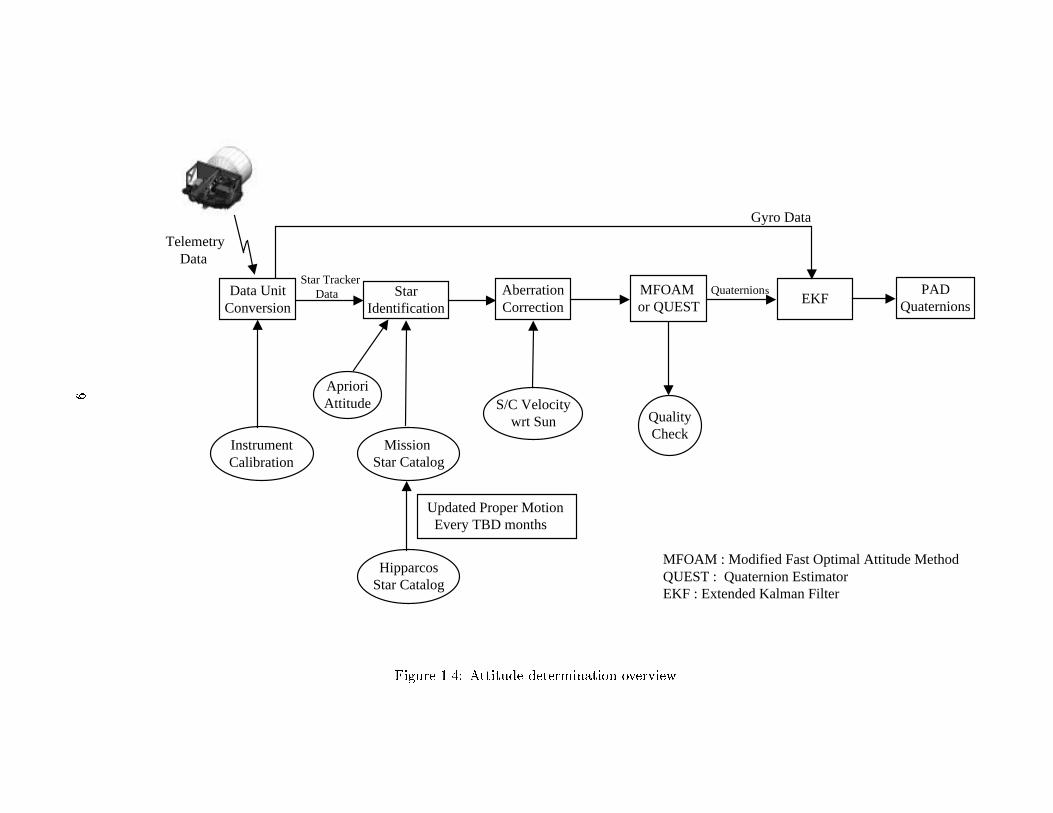
Telemetry Data

Data UnitConversion

StarIdentification

AberrationCorrection

MFOAM or QUEST

EKFPAD

Quaternions

QualityCheck

Mission Star Catalog

HipparcosStar Catalog

S/C Velocitywrt Sun

InstrumentCalibration

Star Tracker Data Quaternions

Gyro Data

Updated Proper Motion Every TBD months

AprioriAttitude

MFOAM : Modified Fast Optimal Attitude MethodQUEST : Quaternion EstimatorEKF : Extended Kalman Filter

Figure 1.4: Attitude determination overview

9

Chapter 2

FUNDAMENTALS OF

ATTITUDE DETERMINATION

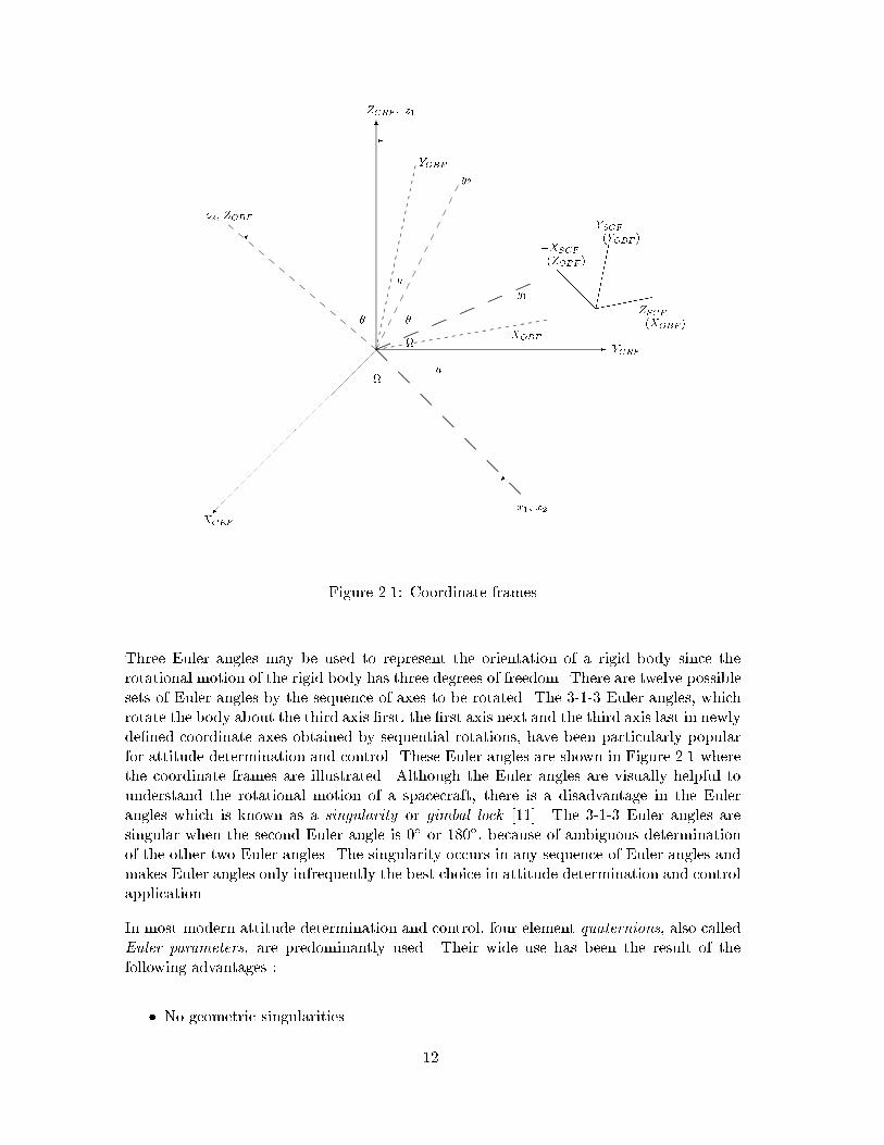
2.1 Coordinate Systems

It is presumed that all of the following coordinate systems have a common origin in thespacecraft except for the Terrestrial Reference Frame. The relevant coordinate systemsare :

� Optical Bench Coordinate Frame (OBF)

The OBF is a coordinate frame �xed in the optical bench and is used to de�nethe optical bench attitude. The origin of the OBF is an instrument reference pointlocated at the optical bench. The orientation of each instrument attached to theoptical bench will usually be described in terms of the OBF. The OBF x-axis isnominally coincident with the optical bench star tracker boresight direction, whichis zenith pointing. The other two axes complete the proper orthogonal system. Theadopted OBF for the GLAS is illustrated in Fig 1.3. To maximize the solar arrays'power generation, the ICESAT will be operated in two nominal attitude modes[29]. The velocity direction of the ICESAT will change between the OBF �z-axisand the �y-axis, controlled by yaw maneuvers. Througout this document, zOBFaxis is perpendicular to the orbital plane (upward) and yOBF completes the properorthogonal system. Since the de�nition of the OBF used here is not the same as thede�nition of the planned OBF in Fig 1.3, the appropriate coordinate transformationshould be applied before actually using the developed algorithm. The angle rotationsabout the (x; y; z)-axes of the OBF are frequently named yaw, roll, and pitch angles,respectively. The term, spacecraft attitude, will actually mean the optical benchattitude for the GLAS instrument in this document.

� Celestial Reference Frame (CRF)The CRF is a non-rotating coordinate frame de�ned by appropriate celestial objects.Ultimately, it is the inertial reference system which all the other coordinate systemsare referred to. The simpli�ed description of the CRF can be : the X axis is to

10

the vernal equinox direction of a speci�ed date, and Y axis is in the equator andthe Z axis completes the proper orthogonal system. The CRF will be realized bythe International Celestial Reference Frame (ICRF) maintained by the InternationalEarth Rotation Service (IERS).

� Star Tracker Coordinate Frame (SCF)The SCF is the coordinate frame �xed to the star tracker mounted on the GLASoptical bench. The direction perpendicular to the star tracker �eld of view (FOV)at the center of it is called the boresight direction (BD). While the narrow FOVstar tracker such as the HD-1003 can give precise knowledge for the direction of theBD vector, it gives relatively poor information about the rotation of the BD vector.For the precise determination of the laser altimeter pointing direction, therefore, theBD of the optical bench star tracker will be aiming at the zenith direction, whichis the opposite direction that laser altimeter will be pointing. For our description,the zSCF is aligned to the BD, the xSCF is toward the orbit normal (downward,being equal to the nominal �zOBF ), and the ySCF completes the proper orthogonalsystem (the nominal yOBF ). The orientation of the SCF with respect to the OBFwill change slowly due to the local deformation of the optical bench and the internalerror of the star tracker itself. The alignment of the SCF in terms of the OBFis assumed to be �xed for the attitude determination process in Chapter 5. Thealignment variations and the corresponding calibrations will be discussed along withthe SRS in Chapter 6.

� Gyro Coordinate Frame (GCF)The de�nition of the GCF is similar to that of the SCF in the sense that the ori-entation is de�ned with respect to the OBF. The GCF may be de�ned by the axesof three orthogonal gyros (usually including a redundant one) in a package, whichis often called the Inertial Reference Unit (IRU). In this document, we simplify theGLAS attitude system by assuming the GCF to be coincident with the OBF. TheGCF and the OBF may not coincide in the real GLAS attitude system, however, theresults from this document will not be a�ected by the change of the GCF orientationwith respect to the OBF, as long as both GCF and OBF are orthogonal coordinatesystems.

� Terrestrial Reference Frame (TRF)The TRF is an Earth-�xed coordinate frame whose origin is coincident with thecenter of mass of the Earth. Ultimately, the laser spot location on the Earth'ssurface will be described in the International Terrestrial Reference Frame (ITRF).

2.2 Quaternion Representation

The attitude of the three axis stabilized spacecraft is most conveniently thought of as arotation matrix which transforms a set of reference axes in inertial space to the axes inthe spacecraft OBF. The rotation matrix is an orthonormal matrix and is also called adirection cosine matrix or an attitude matrix.

11

.

..

.

.

.

..

.

.

.

..

.

.

.

..

.

.

.

..

.

.

.

.

..

.

.

.

..

.

.

..

.

.

..

.

.

.

..

.

.

..

.

.

..

.

.

.

..

.

.

..

.

.

..

.

..

.

.

..

.

.

..

.

..

.

.

..

.

..

.

.

..

.

.

..

.

..

.

..

.

..

.

.

..

.

..

.

..

.

..

.

..

.

..

.

..

.

..

.

..

.

..

.

..

.

..

..

.

..

.

..

.

..

..

.

..

.

..

.

..

..

..

.

..

..

..

..

.

..

..

..

..

.

..

..

..

..

.

..

..

.

..

..

..

.

..

..

..

.

..

..

..

.

..

..

..

.

..

..

.

..

.

..

..

..

.

..

.

..

.

..

..

..

.

..

.

..

.

..

..

.

..

..

..

..

..

.

..

..

.

..

..

..

..

..

.

..

..

..

..

..

..

..

..

..

..

..

..

..

.

..

..

..

..

................................................................................................................................................................................................................................................................................

..................

.....................................

............................................................................................................................................................................................................................................................................................................................................................................

...............................................................................................................................................................................................................................................................................................................................................................................................................................................................................................................................................................................................................................................................................................................................................................................................................................................................................................................................................................................................................................

...................................................................................................................................................................................................................................................................................................................................................................................................................................................................................................................................................................................................................................................................

6

ZCRF , z1

- YCRF��

��

��

���

��

����

XCRF

x1; x2

y1

.............................................................................................

.

..

.

.

.

..

.

.

..

.

.

..

.

..

.

..

.

..

.

.

y2

z2; ZOBF

.

..

..

..

..

..

..

..

..

..

.

..

..

..

..

..

.................................

�..........................................................

�

XOBF

YOBF

..

..

.

..

..

..

.

..

..

..

..

..

..

.

..

..

.

..

..

..

.

..

..

.

..

..

.

..

.

..

..

.

..

.

..

..

.

..

.

..

..

.

..

.

..

.

.

..

.

.

..

.

.

..

.

.

..

.

.

..

.

.

.

.

..

.

.

.

..

.

.

.

.

..

.

.

.

.

..

.

.

.

.

..

.

.

.

..

.

.

.

.

..

.

.

.

..

.

.

.

.

..

.

u

..........................................

u

...................

......................................................................................

.......................................

-

.................................................................................

..

..

..

.

.

..

.

..

.

.

..

..

..

.

..

..

..

.

..

..

.

..

..

.....................

.................................................................................

...........................................................

�

ZSCF(XOBF )

������

YSCF(YOBF )

@@@@

�XSCF(ZOBF )

Figure 2.1: Coordinate frames

Three Euler angles may be used to represent the orientation of a rigid body since therotational motion of the rigid body has three degrees of freedom. There are twelve possiblesets of Euler angles by the sequence of axes to be rotated. The 3-1-3 Euler angles, whichrotate the body about the third axis �rst, the �rst axis next and the third axis last in newlyde�ned coordinate axes obtained by sequential rotations, have been particularly popularfor attitude determination and control. These Euler angles are shown in Figure 2.1 wherethe coordinate frames are illustrated. Although the Euler angles are visually helpful tounderstand the rotational motion of a spacecraft, there is a disadvantage in the Eulerangles which is known as a singularity or gimbal lock [11]. The 3-1-3 Euler angles aresingular when the second Euler angle is 0� or 180�, because of ambiguous determinationof the other two Euler angles. The singularity occurs in any sequence of Euler angles andmakes Euler angles only infrequently the best choice in attitude determination and controlapplication.

In most modern attitude determination and control, four element quaternions, also calledEuler parameters, are predominantly used. Their wide use has been the result of thefollowing advantages :

� No geometric singularities

12

� Rigorous satisfaction of a set of linear di�erential equations.

� No requirement for the evaluation of trigonometric functions

The lack of trigonometric functions in the computation of quaternions is clearly an ad-vantage in time-critical real time operations. Extensive use of trigonometric function inEuler angles will signi�cantly increase the computation time, especially with modest per-formance computers such as those used in on-board applications. The quaternions arede�ned based on Euler's rotation theorem [11] :

The most general displacement of a rigid body with one point �xed is equivalentto a single rotation about some axis through that point.

For some axis, e, and a single rotation angle, ��, the quaternions are de�ned by

q1 = ex sin(��

2)

q2 = ey sin(��

2)

q3 = ez sin(��

2) (2.1)

q4 = cos(��

2)

where ex, ey and ez are components of rotation axes in terms of the OBF before therotation. Since there are only three degrees of freedom for the rotational motion, thefollowing constraint exists in the quaternion representation :

q21 + q22 + q23 + q24 = 1 (2.2)

The single constraint to be observed is a minor disadvantage associated with the fourquaternions. The detailed properties of quaternions and relevant equations are summarizedin Appendix A.

The quaternion errors �q are frequently represented by another quaternion rotation, whichmust be composed with the estimated quaternions q in order to obtain the true quaternionsqtrue as

qtrue = �q q; (2.3)

where the quaternion composition, , is de�ned in Equation A.9. A bene�t of this errorrepresentation can be seen by applying the small angle approximations to Equation 2.1 :

�q1 =�x2

�q2 =�y2

�q3 =�z2

(2.4)

�q4 = 1;

13

where �x, �y, and �z were de�ned in the previous section as yaw, roll, and pitch angles,respectively. Only the vector components of quaternions (see Equation A.1) correspond toangle errors and the scalar component becomes insigni�cant to the �rst order. By applyinginverse quaternions (Equation A.2) to Equation 2.3, the error quaternions are expressedas

�q = qtrue q�1: (2.5)

Even though the Euler angles are not convenient for numerical computations, their geo-metrical signi�cance in illustrating the rotational motion is more apparent than quater-nions. Therefore, they are often used for computer input/output and for analysis. In thisresearch, simulated attitude data were created by Euler angles and, then, converted tothe quaternions using Equation A.13. Euler angles can be recalculated from estimatedquaternions by Equation A.14.

2.3 Kinematic Equations of Spacecraft Attitude

If the quaternion composition (Equation A.9) is performed successively in time, the timeevolution of quaternions during the time interval �t is given by

q(t+�t) = q(�t) q(t): (2.6)

Let !x, !y and !z be the components of angular velocity vector (~!) at time t, j!j bethe magnitude of the angular velocity, and �� be a rotation angle during �t. From thede�nition of quaternions, we can derive

q(t+�t) = [cos(��)

2I4�4 +

sin(��)

2

(~!)

j!j ]q(t); (2.7)

where (~!) is

(~!) �

2664

0 !z �!y !x�!z 0 !x !y!y �!x 0 !z

�!x �!y �!z 0

3775 : (2.8)

This equation predicts the attitude at the future time based on the knowledge of thecurrent attitude if the axis of rotation is invariant over the time interval �t. If the averageor instantaneous angular velocity of a spacecraft is known during �t, the rotation angle is

�� = j!j�t (2.9)

about the rotation axis. Assuming �t is small enough, the small angle approximations

cos��

2� 1; sin

��

2� 1

2!�t (2.10)

14

lead to the attitude di�erential equation

d

dtq(t) =

1

2(!(t))q(t) (2.11)

from Equation 2.7. Equation 2.11 is the fundamental kinematic equation for the attitudedetermination and can be rearranged in a di�erent order such that [6]

d

dtq =

1

2

2664

q4 �q3 q2 q1q3 q4 �q1 q2

�q2 q1 q4 q3�q1 �q2 �q3 q4

37752664

0!x!y!z

3775 : (2.12)

Conversely,

!x = 2(q4 _q1 + q3 _q2 � q2 _q3 � q1 _q4)

!y = 2(�q3 _q1 + q4 _q2 + q1 _q3 � q2 _q4) (2.13)

!z = 2(q2 _q1 � q1 _q2 + q4 _q3 � q3 _q4):

For reference, the 3-1-3 Euler angle representation for angular velocity is

!x = _ sin� sin � + _� cos�

!y = _ cos� sin � � _� sin� (2.14)

!z = _ cos � + _�;

where ; � and � are three Euler angles in the sequential order.

2.4 Dynamical Equations of Spacecraft Attitude

The rotational motion of a body about its center of mass is

d~h

dt= ~T ; (2.15)

where ~T is an applied torque and ~h is an angular momentum vector. With ~h described inthe spacecraft body-�xed axes, it follows that

_~hOBF + ~! � ~hOBF = ~T ; (2.16)

where ~! is again an angular velocity vector. Expanding the above equation gives thegeneral Euler equations of attitude :

_hx + !yhz � !zhy = Tx_hy + !zhx � !xhz = Ty (2.17)

_hz + !xhy � !yhx = Tz;

where hx; hy; hz are the angular momentum components along the OBF, and Tx; Ty; Tzare the body referenced external torque components. For the solution of these equations,

15

the external torque of ~T must be modeled as a function of time as well as a function ofthe position and attitude of the spacecraft. The dominant sources of attitude disturbancetorques are the Earth's gravitational and magnetic �elds, solar radiation pressure, andaerodynamic drag [52].

In many spacecraft, gyros are grouped as an IRU. When the gyros are used to measurethe angular velocity of the spacecraft, the numerical or analytical expression for externaltorques is not necessary. Angular velocities measured by gyros are substituted directly intothe kinematic equation (Equation 2.11) for attitude prediction. Such gyro measurementsactually include the e�ect of all torques acting on the spacecraft. Force model errors inthis situation will exist only to the extent that the measurements from a gyro unit containerrors. Since the HRG will measure the angular rate of the ICESAT, the Euler equationsare not required for the attitude determination. The attitude determination in the eventof gyro failure will be discussed in Chapter 5.

2.5 Attitude Determination Problem

The minimum required knowledge for three-axis attitude determination is the directionvectors to two celestial objects which are represented in the OBF (or the Spacecraft Body-Fixed Coordinate Frame generally) and are also known in the reference frame, such as theCRF. Since the stars are measured in the SCF, the unit vectors in the OBF are determinedusing the rotation matrix between two coordinate systems. Denote the two unit vectormeasurements by W1 and W2 in the OBF and V1 and V2 in the CRF. To obtain V1 andV2, the measured stars in the SCF must be identi�ed in a given star catalog with thestar identi�cation algorithms developed in Chapter 4. A simple attitude determinationproblem is given as :

Find an attitude matrix A, to satisfy

W1 = AV1; W2 = AV2; (2.18)

where the measured vectors and the catalog vectors require

W1 � W2 = V1 � V2 (2.19)

within the measurement and the catalog error bound.

A simple algorithm to �nd the attitude matrix from any two vector measurements iscalled TRIAD [39] or an algebraic method [52]. The method has been applied for atleast three decades and was employed in several missions, usually for coarse attitudedetermination. Whereas it is relatively easy to evaluate the TRIAD attitude matrix, it hasmany disadvantages. The most serious disadvantage might occur when more than threeunit vectors are observed simultaneously, which is a common case in CCD star trackermeasurements. (In Section 4.1, three observation vectors are the minimum number forutilizing a pattern matching algorithm.)

16

To take advantage of multiple unit vectors simultaneously obtained by a CCD star tracker(or the combination of multiple sensors), a least squares attitude problem was suggestedin the early 1960's by Wahba [51]. The well-known Wahba Problem is :

Find the proper orthogonal matrix A that minimizes the loss function, J(A),

J(A) =1

2

nXi=1

aijWi �AVij2; (2.20)

where the unit vectors Vi are representations in a reference frame of the di-rections to some observed objects, the Wi are the unit vector representationsof corresponding observations in the spacecraft body frame, the ai are positiveweights, and n is the number of observations

The Wahba Problem is basically a weighted least squares problem for the attitude matrix,A. It is also known to be equivalent to a maximum likelihood estimation problem for asimple, but realistic probabilistic model for vector measurements [36]. For error-free ob-servations (and also error-free catalog positions), the true attitude matrix Atrue will drivethe loss function, J(A), to be zero. In a practical situation, the A must be found that min-imizes J(A). The solutions of the Wahba Problem, which are deterministic approaches tothe computation of the attitude matrix (or quaternions) will be introduced in Chapter 5.

17

Chapter 3

MEASUREMENT SYSTEM

Many spacecraft use gyro units to continuously measure their angular velocities. Tradi-tional mechanical gyros react to the motion of the host spacecraft based on the principle ofconservation of angular momentum. Non-mechanical gyros have been constructed on phys-ical phenomena such as general relativity or the inertial vibration property of a standingvibration wave on a hemispherical body. Such gyros are usually sensitive to high frequencynoise and able to measure attitude change very accurately. However, slowly drifting gyrobiases will produce deviations of predicted attitude from true attitude. Some externalsources such as the Sun, the Moon, the Earth and stars must be observed in order toprevent gyro biases from deteriorating the attitude determination process based on gyros.Measurements from external sources are relatively insensitive to the high frequency of at-titude change due to instrument noise and jitter. However, such measurements providegood information in the low frequency of attitude motion because the positions of celestialobjects are well-predicted (Sun, Moon, and Earth) or they are essentially �xed in space(stars). Therefore, gyros and sensors for the external sources are generally used togetherin the attitude determination system.

The CCD star tracker which measures multiple stars with a frequency of 10 Hz also enablesangular rate information to be inferred and may be used alone for the accurate attitudedetermination. However, in reality, the high frequency jitter in the spacecraft motion, theirregular distribution of stars, CCD limitations for data read-out and the blockage of starmeasurements due to the Sun or the Moon require measurements of the spacecraft angularvelocity from gyros for continuous attitude determination.

This chapter introduces CCD star trackers and gyros which will be used in the ICE-SAT/GLAS. In addition, a star catalog which is an essential component of the attitudedetermination using star sensors will be discussed.

3.1 CCD Star Tracker

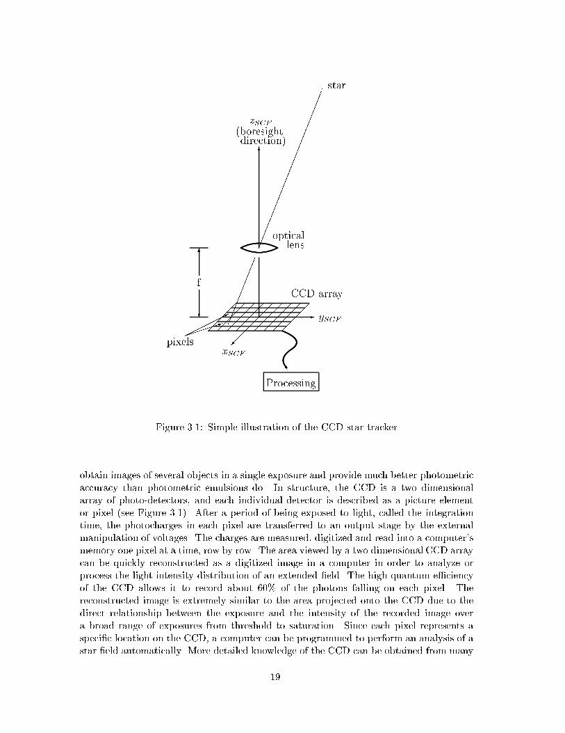
The CCD image detector was developed in 1970 by Boyle and Smith at Bell Laboratories[4]. Unlike the traditional light detectors, two-dimensional CCD detectors allow one to

18

p star

6

zSCF

(boresightdirection)

opticallens

���

���

CCD array

��������

������������������

p

- ySCF��

�xSCF

6

?

f

���

���

���

���

���

���

���

�����*

����1

pixels

U

Processing

Figure 3.1: Simple illustration of the CCD star tracker

obtain images of several objects in a single exposure and provide much better photometricaccuracy than photometric emulsions do. In structure, the CCD is a two dimensionalarray of photo-detectors, and each individual detector is described as a picture elementor pixel (see Figure 3.1). After a period of being exposed to light, called the integrationtime, the photocharges in each pixel are transferred to an output stage by the externalmanipulation of voltages. The charges are measured, digitized and read into a computer'smemory one pixel at a time, row by row. The area viewed by a two dimensional CCD arraycan be quickly reconstructed as a digitized image in a computer in order to analyze orprocess the light intensity distribution of an extended �eld. The high quantum e�ciencyof the CCD allows it to record about 60% of the photons falling on each pixel. Thereconstructed image is extremely similar to the area projected onto the CCD due to thedirect relationship between the exposure and the intensity of the recorded image overa broad range of exposures from threshold to saturation. Since each pixel represents aspeci�c location on the CCD, a computer can be programmed to perform an analysis of astar �eld automatically. More detailed knowledge of the CCD can be obtained from many

19

sources [4] [14] [44].

In space applications, CCDs have been used on many imaging missions including theHubble Space Telescope. The CCD star tracker was developed in the late 1970's and ithas recently begun to be used in space missions as a component in state-of-the-art attitudedetermination hardware. The traditional star sensor detects only one or two stars in itsFOV, and therefore, has been used with other types of attitude hardware like Sun sensors,horizon sensors or magnetometers. Since the CCD star tracker observes multiple starssimultaneously, it is sometimes referred to as a star camera and some spacecraft use aCCD star tracker as the sole attitude sensor except for initial attitude acquisition in realtime applications. Even though the initial attitude acquisition may require other sensorsfor coarse attitude determination, this may be also performed by a star tracker with awide FOV [26] [17]. A simpli�ed illustration of the CCD array and lens in the star trackeris shown in Figure 3.1. The following sections describe characteristics of commerciallyavailable CCD star trackers.

3.1.1 HD-1003 Star Tracker

For the PAD of the GLAS, the Raytheon Optical System Inc.(ROSI) HD-1003 [5], a CCDstar tracker, will be mounted on the instrument optical bench. It is an electro-opticalsensor that implements CCD array detectors to search for and track up to six stars in an8�� 8� FOV with an array of 512 � 512 pixels. The star tracker operates at a 10 Hz rate,thereby measuring coordinates of tracking stars as well as their light intensities every 0.1second. It provides the position of a star with a six arcseconds (1�) error in each axis ofpitch and roll. A magnitude measurement is given within 0.2 magnitude (1�) uncertainty.The nominal sensitivity range of the star magnitude is between 2.0 and 6.0. Functionally,the HD-1003 star tracker is operated in search and track mode. The star tracker searchesthe entire FOV to �nd the six brightest stars in search mode. After acquisition, it continuestracking these stars and periodically computes updated angular positions as the stars passacross the FOV in track mode. The performance characteristics of the ROSI HD-1003 aresummarized and compared to the characteristics of the Ball CT-601 and the LockheedAST in Table 3.1.

The HD-1003 star tracker manufactured by Raytheon for GLAS was tested during theperiod between summer 1999 and spring 2000. Various tests were conducted, such asmechanical properties measurement, spectral calibration, thermal vacuum segment andacceptance vibration. Table 3.2 shows the results of the �nal performance test whichwas performed in an air conditioned room after electronics and software upgrades [7].The static accuracy test measures the position accuracy of stars that are �xed relativeto the tracker. The dynamic accuracy test measures the star location accuracy whiletracking a moving star at a rate of 0.20 deg/second. The table presents only the post-vibration results, but the pre-vibration results showed similar values. All requirementswere reported to have been met based on the pass/fail criteria speci�ed in both pre/postvibration. The overall performance of the HD-1003 was not compromised by exposureto the random vibration, thermal or vacuum environment. After the �nal performancetest, point sources were generated by the Scene Simulator computer in order to simulate

20

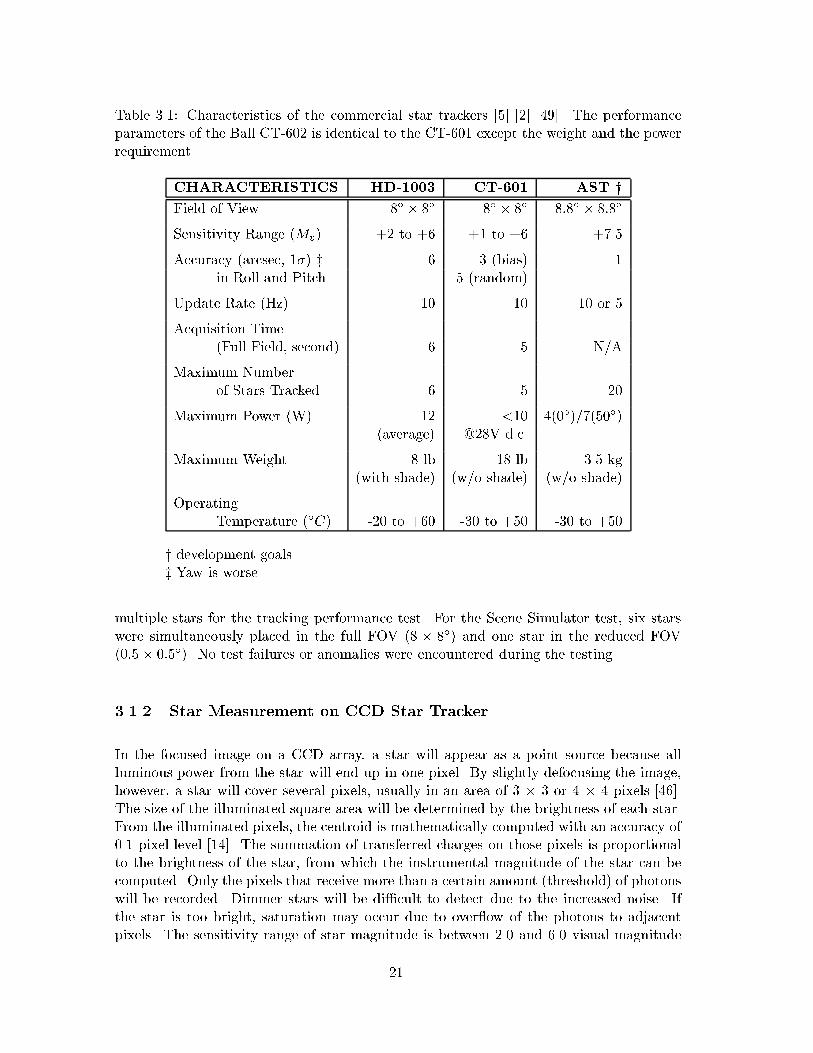
Table 3.1: Characteristics of the commercial star trackers [5] [2] [49]. The performanceparameters of the Ball CT-602 is identical to the CT-601 except the weight and the powerrequirement.

CHARACTERISTICS HD-1003 CT-601 AST y

Field of View 8� � 8� 8� � 8� 8:8� � 8:8�

Sensitivity Range (Mv) +2 to +6 +1 to +6 +7.5

Accuracy (arcsec, 1�) z 6 3 (bias) 1in Roll and Pitch 5 (random)

Update Rate (Hz) 10 10 10 or 5

Acquisition Time(Full Field, second) 6 5 N/A

Maximum Numberof Stars Tracked 6 5 20

Maximum Power (W) 12 <10 4(0�)/7(50�)(average) @28V d.c.

Maximum Weight 8 lb 18 lb 3.5 kg(with shade) (w/o shade) (w/o shade)

OperatingTemperature (�C) -20 to +60 -30 to +50 -30 to +50

y development goalsz Yaw is worse

multiple stars for the tracking performance test. For the Scene Simulator test, six starswere simultaneously placed in the full FOV (8 � 8�) and one star in the reduced FOV(0:5 � 0:5�). No test failures or anomalies were encountered during the testing.

3.1.2 Star Measurement on CCD Star Tracker

In the focused image on a CCD array, a star will appear as a point source because allluminous power from the star will end up in one pixel. By slightly defocusing the image,however, a star will cover several pixels, usually in an area of 3 � 3 or 4 � 4 pixels [46].The size of the illuminated square area will be determined by the brightness of each star.From the illuminated pixels, the centroid is mathematically computed with an accuracy of0.1 pixel level [14]. The summation of transferred charges on those pixels is proportionalto the brightness of the star, from which the instrumental magnitude of the star can becomputed. Only the pixels that receive more than a certain amount (threshold) of photonswill be recorded. Dimmer stars will be di�cult to detect due to the increased noise. Ifthe star is too bright, saturation may occur due to over ow of the photons to adjacentpixels. The sensitivity range of star magnitude is between 2.0 and 6.0 visual magnitude

21

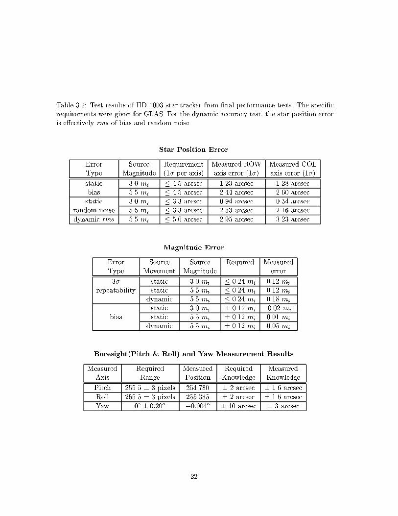
Table 3.2: Test results of HD-1003 star tracker from �nal performance tests. The speci�crequirements were given for GLAS. For the dynamic accuracy test, the star position erroris e�ectively rms of bias and random noise.

Star Position Error

Error Source Requirement Measured ROW Measured COLType Magnitude (1� per axis) axis error (1�) axis error (1�)

static 3.0 mi � 4.5 arcsec 1.23 arcsec 1.28 arcsecbias 5.5 mi � 4.5 arcsec 2.44 arcsec 2.60 arcsec

static 3.0 mi � 3.3 arcsec 0.94 arcsec 0.54 arcsecrandom noise 5.5 mi � 3.3 arcsec 2.53 arcsec 2.16 arcsec

dynamic rms 5.5 mi � 5.0 arcsec 2.95 arcsec 3.23 arcsec

Magnitude Error

Error Source Source Required MeasuredType Movement Magnitude error

3� static 3.0 mi � 0.24 mi 0.12 mi

repeatability static 5.5 mi � 0.24 mi 0.12 mi

dynamic 5.5 mi � 0.24 mi 0.18 mi

static 3.0 mi � 0.12 mi -0.02 mi

bias static 5.5 mi � 0.12 mi 0.01 mi

dynamic 5.5 mi � 0.12 mi 0.05 mi

Boresight(Pitch & Roll) and Yaw Measurement Results

Measured Required Measured Required MeasuredAxis Range Position Knowledge Knowledge

Pitch 255.5 � 3 pixels 254.780 � 2 arcsec � 1.6 arcsec

Roll 255.5 � 3 pixels 255.385 � 2 arcsec � 1.6 arcsec

Yaw 0� � 0:20� �0:004� � 10 arcsec � 3 arcsec

22

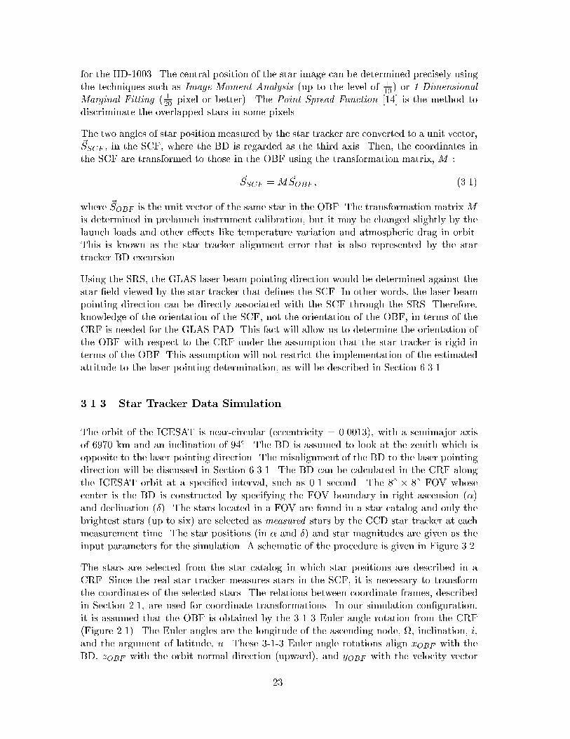
for the HD-1003. The central position of the star image can be determined precisely usingthe techniques such as Image Moment Analysis (up to the level of 1

10) or 1-DimensionalMarginal Fitting ( 1

20 pixel or better). The Point Spread Function [14] is the method todiscriminate the overlapped stars in some pixels.

The two angles of star position measured by the star tracker are converted to a unit vector,~SSCF , in the SCF, where the BD is regarded as the third axis. Then, the coordinates inthe SCF are transformed to those in the OBF using the transformation matrix, M :

~SSCF =M~SOBF ; (3.1)

where ~SOBF is the unit vector of the same star in the OBF. The transformation matrixMis determined in prelaunch instrument calibration, but it may be changed slightly by thelaunch loads and other e�ects like temperature variation and atmospheric drag in orbit.This is known as the star tracker alignment error that is also represented by the startracker BD excursion.

Using the SRS, the GLAS laser beam pointing direction would be determined against thestar �eld viewed by the star tracker that de�nes the SCF. In other words, the laser beampointing direction can be directly associated with the SCF through the SRS. Therefore,knowledge of the orientation of the SCF, not the orientation of the OBF, in terms of theCRF is needed for the GLAS PAD. This fact will allow us to determine the orientation ofthe OBF with respect to the CRF under the assumption that the star tracker is rigid interms of the OBF. This assumption will not restrict the implementation of the estimatedattitude to the laser pointing determination, as will be described in Section 6.3.1.

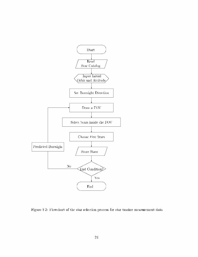
3.1.3 Star Tracker Data Simulation

The orbit of the ICESAT is near-circular (eccentricity = 0.0013), with a semimajor axisof 6970 km and an inclination of 94�. The BD is assumed to look at the zenith which isopposite to the laser pointing direction. The misalignment of the BD to the laser pointingdirection will be discussed in Section 6.3.1. The BD can be calculated in the CRF alongthe ICESAT orbit at a speci�ed interval, such as 0.1 second. The 8� � 8� FOV whosecenter is the BD is constructed by specifying the FOV boundary in right ascension (�)and declination (�). The stars located in a FOV are found in a star catalog and only thebrightest stars (up to six) are selected as measured stars by the CCD star tracker at eachmeasurement time. The star positions (in � and �) and star magnitudes are given as theinput parameters for the simulation. A schematic of the procedure is given in Figure 3.2.

The stars are selected from the star catalog in which star positions are described in aCRF. Since the real star tracker measures stars in the SCF, it is necessary to transformthe coordinates of the selected stars. The relations between coordinate frames, describedin Section 2.1, are used for coordinate transformations. In our simulation con�guration,it is assumed that the OBF is obtained by the 3-1-3 Euler angle rotation from the CRF(Figure 2.1). The Euler angles are the longitude of the ascending node, , inclination, i,and the argument of latitude, u. These 3-1-3 Euler angle rotations align xOBF with theBD, zOBF with the orbit normal direction (upward), and yOBF with the velocity vector

23

��

��Start

?

����

����Read

Star Catalog

?

��

@@

@@

��

Input Initial

Orbit and Attitude

?

Set Boresight Direction

?

Draw a FOV

?

Select Stars inside the FOV

?

Choose Five Stars

?

����

����

Store Stars

?

����

�HHHHHHHHHH����

�End Condition?

?��

��End

Yes

No

Predicted Boresight

-

Figure 3.2: Flowchart of the star selection process for star tracker measurement data

24

direction. The SCF is obtained by simple rotation about yOBF to make the zSCF to bethe BD of star tracker.

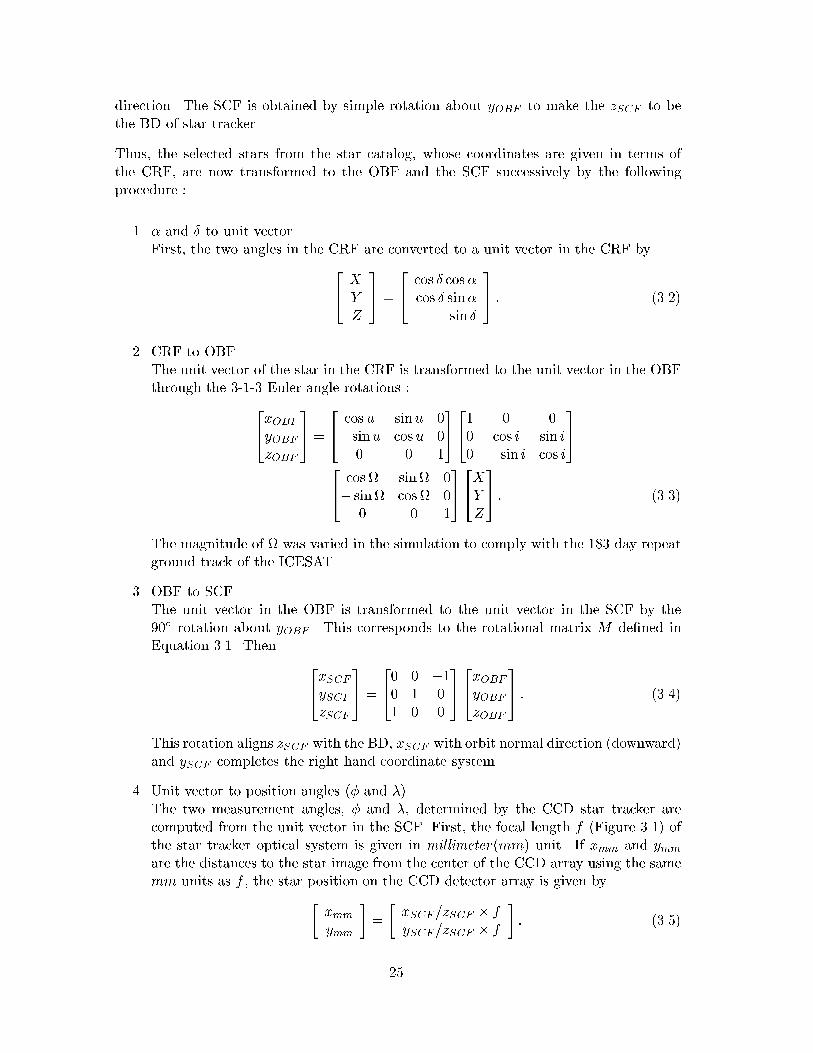
Thus, the selected stars from the star catalog, whose coordinates are given in terms ofthe CRF, are now transformed to the OBF and the SCF successively by the followingprocedure :

1. � and � to unit vectorFirst, the two angles in the CRF are converted to a unit vector in the CRF by2

4 XYZ

35 =

24 cos � cos�

cos � sin�sin �

35 : (3.2)

2. CRF to OBFThe unit vector of the star in the CRF is transformed to the unit vector in the OBFthrough the 3-1-3 Euler angle rotations :2

4xOBFyOBFzOBF

35 =

24 cos u sinu 0� sinu cos u 0

0 0 1

35241 0 00 cos i sin i0 � sin i cos i

35

24 cos sin 0� sin cos 0

0 0 1

3524XYZ

35 : (3.3)

The magnitude of was varied in the simulation to comply with the 183 day repeatground track of the ICESAT.

3. OBF to SCFThe unit vector in the OBF is transformed to the unit vector in the SCF by the90� rotation about yOBF . This corresponds to the rotational matrix M de�ned inEquation 3.1. Then 2

4xSCFySCFzSCF

35 =

240 0 �10 1 01 0 0

3524xOBFyOBFzOBF

35 : (3.4)

This rotation aligns zSCF with the BD, xSCF with orbit normal direction (downward)and ySCF completes the right hand coordinate system.

4. Unit vector to position angles (� and �)The two measurement angles, � and �, determined by the CCD star tracker arecomputed from the unit vector in the SCF. First, the focal length f (Figure 3.1) ofthe star tracker optical system is given in millimeter(mm) unit. If xmm and ymm

are the distances to the star image from the center of the CCD array using the samemm units as f , the star position on the CCD detector array is given by�

xmm

ymm

�=

�xSCF=zSCF � fySCF=zSCF � f

�: (3.5)

25

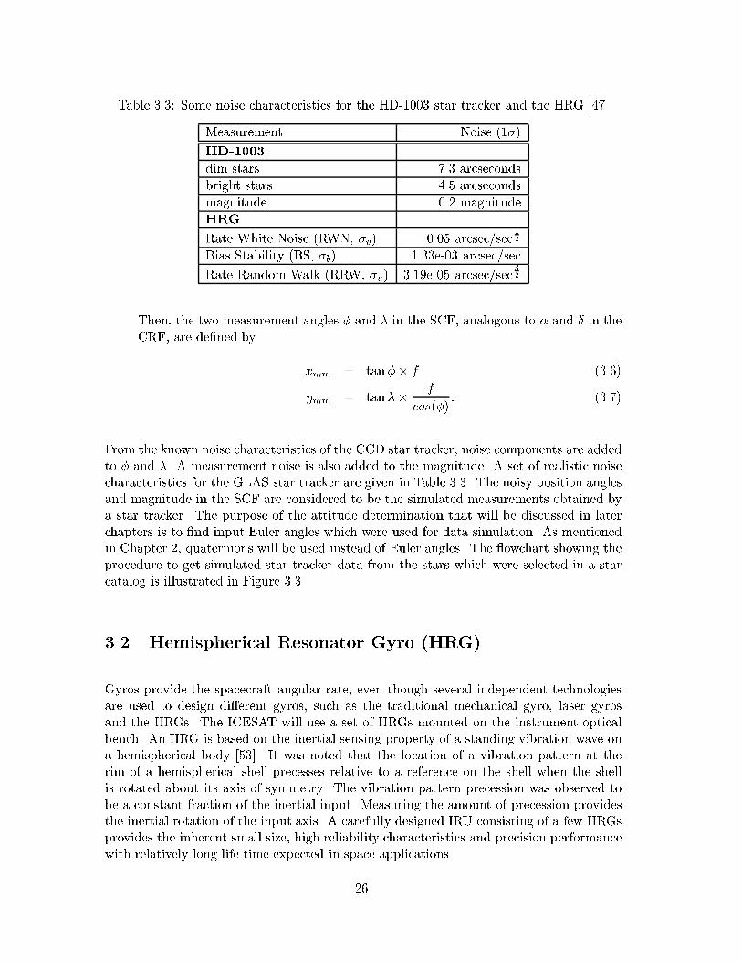
Table 3.3: Some noise characteristics for the HD-1003 star tracker and the HRG [47]

Measurement Noise (1�)

HD-1003

dim stars 7.3 arcseconds

bright stars 4.5 arcseconds

magnitude 0.2 magnitude

HRG

Rate White Noise (RWN, �v) 0.05 arcsec/sec1

2

Bias Stability (BS, �b) 1.33e-03 arcsec/sec

Rate Random Walk (RRW, �u) 3.19e-05 arcsec/sec3

2

Then, the two measurement angles � and � in the SCF, analogous to � and � in theCRF, are de�ned by

xmm = tan�� f (3.6)

ymm = tan �� f

cos(�): (3.7)

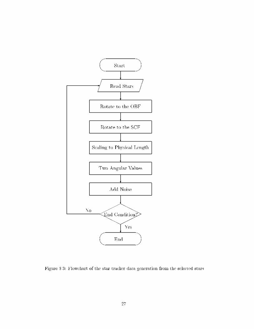
From the known noise characteristics of the CCD star tracker, noise components are addedto � and �. A measurement noise is also added to the magnitude. A set of realistic noisecharacteristics for the GLAS star tracker are given in Table 3.3. The noisy position anglesand magnitude in the SCF are considered to be the simulated measurements obtained bya star tracker. The purpose of the attitude determination that will be discussed in laterchapters is to �nd input Euler angles which were used for data simulation. As mentionedin Chapter 2, quaternions will be used instead of Euler angles. The owchart showing theprocedure to get simulated star tracker data from the stars which were selected in a starcatalog is illustrated in Figure 3.3.

3.2 Hemispherical Resonator Gyro (HRG)

Gyros provide the spacecraft angular rate, even though several independent technologiesare used to design di�erent gyros, such as the traditional mechanical gyro, laser gyrosand the HRGs. The ICESAT will use a set of HRGs mounted on the instrument opticalbench. An HRG is based on the inertial sensing property of a standing vibration wave ona hemispherical body [53]. It was noted that the location of a vibration pattern at therim of a hemispherical shell precesses relative to a reference on the shell when the shellis rotated about its axis of symmetry. The vibration pattern precession was observed tobe a constant fraction of the inertial input. Measuring the amount of precession providesthe inertial rotation of the input axis. A carefully designed IRU consisting of a few HRGsprovides the inherent small size, high reliability characteristics and precision performancewith relatively long life time expected in space applications.

26

��

��Start

?

����

����

Read Stars

?

Rotate to the OBF

?

Rotate to the SCF

?

Scaling to Physical Length

?

Two Angular Values

?

Add Noise

?

����

�HHHHHHHHHH����

�End Condition?

?��

��End

Yes

No

-

Figure 3.3: Flowchart of the star tracker data generation from the selected stars

27

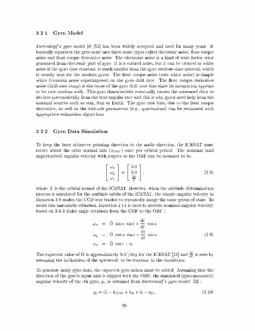
3.2.1 Gyro Model

Farrenkopf's gyro model [8] [52] has been widely accepted and used for many years. Itbasically separates the gyro noise into three noise types called electronic noise, oat torquenoise and oat torque derivative noise. The electronic noise is a kind of scale factor errorgenerated from electronic part of gyro. It is a colored noise, but it can be treated as whitenoise if the gyro time constant is much smaller than the gyro readout time interval, whichis usually true for the modern gyros. The oat torque noise (rate white noise) is simplewhite Gaussian noise superimposed on the gyro drift rate. The oat torque derivativenoise (drift rate ramp) is the cause of the gyro drift rate bias since its integration appearsto be rate random walk. This gyro characteristic eventually causes the measured data todeviate systematically from the true angular rate and this is why gyros need help from theexternal sources such as star, Sun or Earth. The gyro rate bias, due to the oat torquederivative, as well as the attitude parameters (e.g., quaternions) can be estimated withappropriate estimation algorithms.

3.2.2 Gyro Data Simulation

To keep the laser altimeter pointing direction to the nadir direction, the ICESAT mustrotate about the orbit normal axis (zOBF ) once per orbital period. The nominal (andunperturbed) angular velocity with respect to the OBF can be assumed to be

24 !x!y!z

35 =

24 0:00:02�T

35 ; (3.8)

where T is the orbital period of the ICESAT. However, when the attitude determinationprocess is simulated for the multiple orbits of the ICESAT, the simple angular velocity inEquation 3.8 makes the CCD star tracker to repeatedly image the same group of stars. Toavoid this unrealistic situation, Equation 2.14 is used to provide nominal angular velocity,based on 3-1-3 Euler angle rotations from the CRF to the OBF :

!x = _ sinu sin i+di

dtcos u

!y = _ cos u sin i� di

dtsinu (3.9)

!z = _ cos i+ _u:

The expected value of _ is approximately 0:5�=day for the ICESAT [19] and didt is zero by

assuming the inclination of the spacecraft to be constant in the simulation.

To generate noisy gyro data, the expected gyro noises must be added. Assuming that thedirection of the gyro's input axis is aligned with the OBF, the simulated (gyro-measured)angular velocity of the ith gyro, gi, is obtained from Farrenkopf's gyro model [52] :

gi = (1 + ki)!i + bi0 + bi + �i1; (3.10)

28

where ki is a scale factor error, !i is a true or nominal angular velocity, bi0 is an initial biaserror, bi is a gyro bias which is slowly varying in the orbit and �i1 is a white noise on gyrorate. The scale factor relates the gyro output counts to the physical unit measurements andis a function of the angular rate. Assuming that the ki!i term is negligible in comparisonwith bi0 and bi, Equation 3.10 reduces the gyro noise into white noise and random walk(non-white noise) components.

If the gyro measurement vector, ~g, is measured in the GCF while other vectors are de-scribed in the OBF, then the vector form of Equation 3.10 becomes

~g = G (~! +~b0 +~b+ ~�1); (3.11)

where ~! is the nominal spacecraft angular velocity vector in the OBF and G is an orthog-onal matrix transforming the OBF into the GCF. The time varying gyro bias, ~b, can beobtained by the following shaping �lter :

d~b

dt= ~�2; (3.12)

where ~�2 is another white noise uncorrelated to ~�1.

The noise characteristics of HRG under consideration for the ICESAT are given in Ta-ble 3.3. The components of Equation 3.11, such as ~�1, ~b0, and ~b, can be derived from thesevalues.

3.3 Star Catalog

3.3.1 Star Catalog for Star Field Simulation

The star catalog is a fundamental part of the attitude determination process that usesmeasurement data obtained from any type of star sensor. For the star �eld simulation,a star catalog, originally developed to support a spacecraft equipped with a Ball CT-601star tracker, was obtained from the Smithsonian Astrophysical Observatory [43]. The starcatalog contains 4853 stars and is a subset of Yale Bright Star Catalog. Two years of orbitsimulation of ICESAT sampled the entire celestial sphere because of the complete rotationof node through 360�. The probabilities of a certain number of stars being in a FOV usingthe Poisson distribution and the computer simulation are presented in Table 3.4. Fromthe main purpose of the GLAS mission, which measures ice sheet elevation over Greenlandand Antarctica, the distribution of stars in both polar regions (above 60� and below �60�of declination) is more important than any other regions. Therefore the independentcomputations for polar regions were performed and presented in the table. The numberof stars in each polar region is given in the parenthesis. If the distribution of stars wereideally uniform in the star catalog, the star tracker would observe seven or eight catalogstars in each image. However, the non-uniform distribution of stars in the star catalog(and on the celestial sphere) gives many di�erent numbers of stars in each image as shownin Table 3.4. If there are more than six stars in the HD-1003 star tracker FOV, the built-inprocessor may select only six of them in terms of their brightness or relative positions. If

29

Table 3.4: Probability of the number of stars in a FOV

Whole Sky(4853) South Pole(391) North Pole(323)

Stars Poisson Computer Poisson Computer Poisson Computerdist.(%) Simul.(%) dist.(%) Simul.(%) dist.(%) Simul.(%)

� 2 2.0 3.9 0.6 2.8 2.1 1.13 3.8 5.5 1.4 3.2 3.9 2.84 7.2 8.6 3.3 6.0 7.4 8.45 10.8 11.6 5.9 9.5 11.0 12.5� 6 76.2 70.4 88.8 78.5 75.6 75.2

there are one or two stars, the stars still can be identi�ed using the direct match technique(DMT) which will be introduced in Chapter 4. However, the accuracy of the determinedattitude is lower than that obtained from more stars. An approximate relation betweenthe number of stars and the attitude determined by a deterministic method is [18] :

�pd =�starpNFOV

; (3.13)

where �pd is the accuracy of the pointing direction perpendicular to the detector plane,�star is the uncertainty of the star position and NFOV is the number of stars in the FOV.

In the simulation, no cases occurred when no star was observed in the FOV. However,eclipses by the Sun or the Moon can produce periods with no star observations. Theapproximate ranges where the star tracker is adversely a�ected are approximately a 35�

radius from the Sun and a 25� radius from the Moon [5]. For example, the 35� radiusfrom the Sun may cause the maximum eclipse period of about 19 minutes. During theeclipses by the Sun or the Moon, the attitude determination based on the star trackermeasurement is not available and then the attitude changes need to be detected by a setof gyros (e.g., IRU) until new star measurements are obtained in the FOV. However, if thetime duration in which only gyro measurements are available is too long, the intrinsic biasdrift of gyros will cause a signi�cant deviation of the determined attitude from the truth.To reduce the in uence of the Sun and the Moon, the ICESAT/GLAS PAD could use BallCT-602 star trackers whose BDs are tilted in terms of the HD-1003. In the low declinationthe eclipsing due to the Sun and the Moon would be forecasted and pre-considered, butthe low latitude region requires relatively relaxed attitude accuracy. For the ice-sheetmeasurements in polar regions, solar and lunar eclipsing will not raise a serious problembecause the Sun and the Moon are located in low declination (�30� < � < 30�). Planetsare also positioned on or near the ecliptic plane and their movements are well predicted.Thus, planetary obscuration will be dealt with in a similar manner to eclipses by the Sunand the Moon.

3.3.2 Star Catalog for Real Application

For the PAD, the recently completed Hipparcos Star Catalog [1], containing the mostaccurate astrometric and photometric star data compared with other star catalogs, will

30

Table 3.5: Speci�cations of the Hipparcos Star Catalog [1]

Measurement Satellite Hipparcos Satellite(ESA)

Measurement Period 1989.85-1993.21

Number of entries 118218

Catalogue epoch J2000

Reference system ICRS

Date Published June 1997

Astrometry (Hp < 9mag)

Median precision of positions, J1991.25 0.77/0.64 mas (RA/dec)

Median precision of parallaxes 0.97 mas

Median precision of proper motions 0.88/0.74 mas/yr (RA/dec)

Estimated systematic errors < 0.1 mas

Photometry (Hp < 9mag)

Median photometric precision 0.0015 mag

Mean number of photometric observations

per star 110

Number of entries variable

or possibly variable 11597

Number of solved or suspected

double/multiple systems 23882

be used. The median precision of position and brightness of the Hipparcos Star Catalogare 0.77 milliarcsecond and 0.0015 magnitude respectively. (A high proportion of theastrometric data in the recent version (Version 2) of the SKY2000 Master Catalog comesfrom the Hipparcos Star Catalog and the Tycho Catalog that is also the output from ESA'sHipparcos mission.) The important features of the Hipparcos Star Catalog are given inTable 3.5.

3.3.3 Corrections of Star Measurement

Aberration

Aberration is the apparent shift in the position of a star caused by the motion of thespacecraft. For Earth-orbiting spacecraft, the motion of the Earth around the Sun causesa maximum aberration of about 20 arcseconds. The motion of the spacecraft about theEarth at a 600 km altitude with a circular orbit accounts for about 6 arcseconds additionalaberration. The aberration angle, �, is computed from the spacecraft velocity relative to

31

the Sun, ~v, by [52],

� =j~vjcsin �; (3.14)

where c is the speed of light and � is the angular separation between ~v and the true stardirection. Because we need information for all directions, the vector form of aberrationequation is necessary. By using the nutation angles, the aberration vector, ~�, and trueobliquity of the ecliptic, the unit vector direction to the star corrected for annual aberration,SA, is [41]

SA = (1 + ST � ~�)ST � �; (3.15)

where ST is the unit vector to the star rotated into true-of-date coordinates from the unitstar vector in mean equatorial coordinates of date. The aberration due to the spacecraftmotion around the Earth is approximately computed from

S = (1� SA � ~v=c)SA + ~v=c; (3.16)

where S is the unit vector to the apparent place of the star observed by the star sensor inthe spacecraft. The aberration correction is applied right after the star identi�cation.

Proper Motion

Many stars show continuous changes in position indicating a certain angular velocity. Suchangular velocities are known as proper motions. The proper motion of an individual starmay be as large as several arcseconds per year. Special considerations must be given tothe stars which will show signi�cant changes during the mission period due to large propermotions.

Parallax

The star catalog is usually created in the heliocentric inertial coordinate system. Since theEarth is moving around the Sun once a year, the direction of a star as seen from the Earth(and the spacecraft) is changing periodically and half of the changed angle is called parallax.For the GLAS mission, the corrections to the parallax are not required since the maximumparallaxes for the very few closest stars to the solar system are only 0.8 arcsecond andparallaxes of most stars are negligible. Furthermore, the attitude determination is basedon all the stars in the FOV so that the parallax error on one or two stars will not a�ectthe result signi�cantly [18].

32

Chapter 4

STAR IDENTIFICATION

An essential component of CCD star tracker data processing is the star identi�cation.Star measurement data must be identi�ed using the star information in the mission starcatalog to determine exactly which stars the sensor is tracking. Star identi�cation al-gorithms require appropriate parameter adjustment depending on sensor characteristics,noise environments, and the given star catalog. There are several existing star identi�ca-tion techniques [52]. In the �rst section of this chapter, we will discuss a pattern matchingalgorithm (PMA), which matches the angular distances between pairs of observed starswith those of cataloged stars. Since the CCD star tracker enables us to detect multi-ple stars simultaneously, it seems appropriate to choose the PMA as a star identi�cationmethod. An advantage of PMA is that this method can be used when no a priori attitude(or star) information is obtainable or the quality of the a priori information is in doubt.However, the PMA developed for this research requires at least three stars at a measure-ment time, but the simulation sometimes showed that only one or two stars were observedin a star tracker FOV. The second section of this chapter will discuss the DMT, whichidenti�es every measured star separately in the star catalog. Since the ICESAT/GLASwill stay in the simple nadir pointing attitude mode and will estimate the attitude withone arcsecond accuracy at the measurement time, the predicted attitude would be closeto the true attitude. In other words, we have good prediction for star positions at the newmeasurement time and then the area to be searched for in order to �nd the matched starshould be small. In this way, it is possible to identify most of the measured stars, evenwhen one or two stars are observed by the star tracker. The DMT could be used as theauxiliary method to help the PMA, but it could also be used as stand-alone method if theBD would be known all the time with su�ciently good accuracy either from the attitudeprediction or from real time on-board attitude determination.

33

4.1 Pattern Matching Algorithm

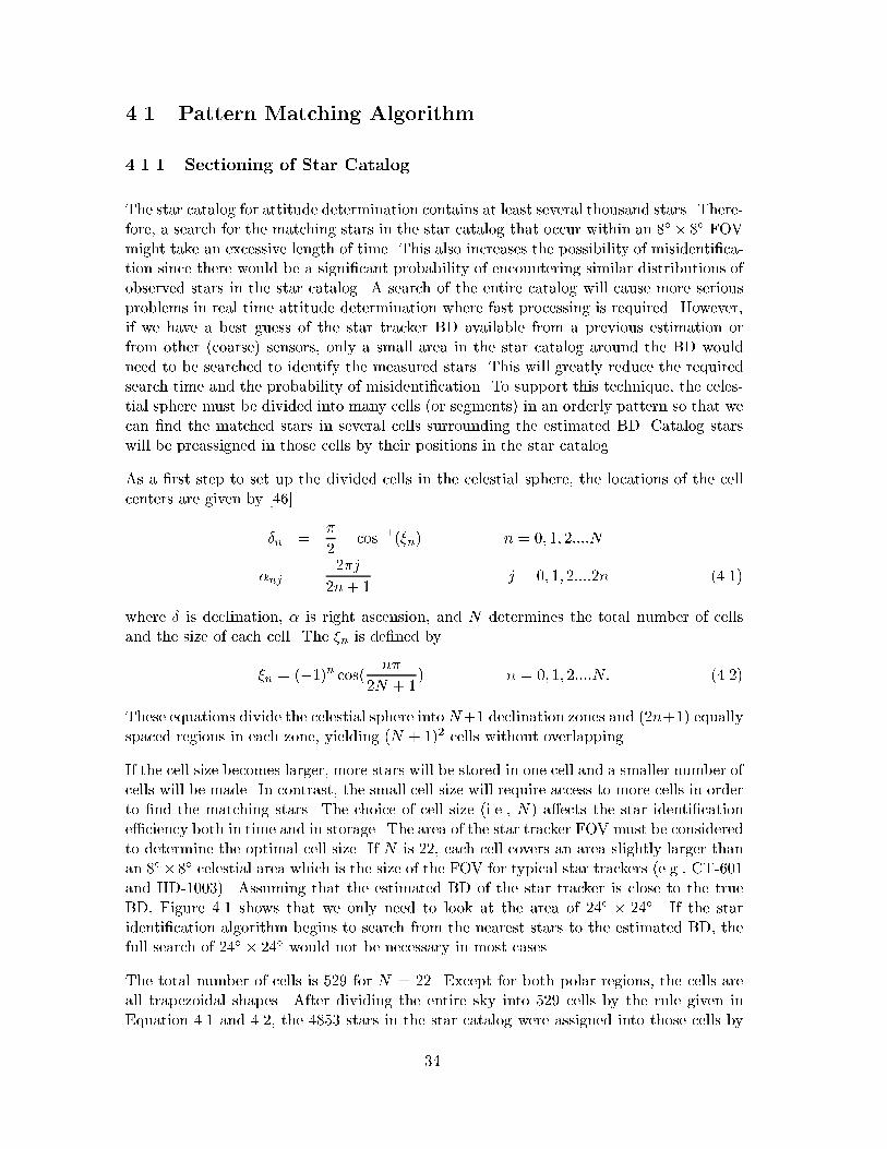
4.1.1 Sectioning of Star Catalog

The star catalog for attitude determination contains at least several thousand stars. There-fore, a search for the matching stars in the star catalog that occur within an 8� � 8� FOVmight take an excessive length of time. This also increases the possibility of misidenti�ca-tion since there would be a signi�cant probability of encountering similar distributions ofobserved stars in the star catalog. A search of the entire catalog will cause more seriousproblems in real time attitude determination where fast processing is required. However,if we have a best guess of the star tracker BD available from a previous estimation orfrom other (coarse) sensors, only a small area in the star catalog around the BD wouldneed to be searched to identify the measured stars. This will greatly reduce the requiredsearch time and the probability of misidenti�cation. To support this technique, the celes-tial sphere must be divided into many cells (or segments) in an orderly pattern so that wecan �nd the matched stars in several cells surrounding the estimated BD. Catalog starswill be preassigned in those cells by their positions in the star catalog.

As a �rst step to set up the divided cells in the celestial sphere, the locations of the cellcenters are given by [46]

�n =�

2� cos�1(�n) n = 0; 1; 2::::N

�nj =2�j

2n+ 1j = 0; 1; 2::::2n (4.1)

where � is declination, � is right ascension, and N determines the total number of cellsand the size of each cell. The �n is de�ned by

�n = (�1)n cos( n�

2N + 1) n = 0; 1; 2::::N: (4.2)

These equations divide the celestial sphere into N+1 declination zones and (2n+1) equallyspaced regions in each zone, yielding (N + 1)2 cells without overlapping.

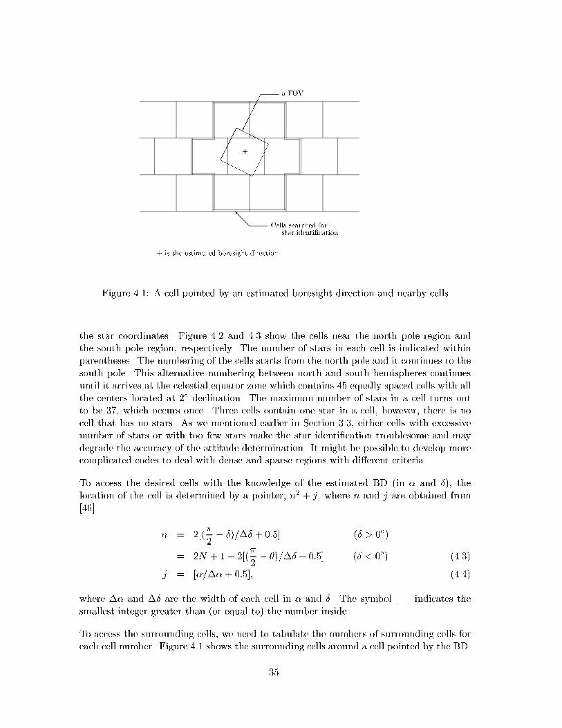
If the cell size becomes larger, more stars will be stored in one cell and a smaller number ofcells will be made. In contrast, the small cell size will require access to more cells in orderto �nd the matching stars. The choice of cell size (i.e., N) a�ects the star identi�catione�ciency both in time and in storage. The area of the star tracker FOV must be consideredto determine the optimal cell size. If N is 22, each cell covers an area slightly larger thanan 8��8� celestial area which is the size of the FOV for typical star trackers (e.g., CT-601and HD-1003). Assuming that the estimated BD of the star tracker is close to the trueBD, Figure 4.1 shows that we only need to look at the area of 24� � 24�. If the staridenti�cation algorithm begins to search from the nearest stars to the estimated BD, thefull search of 24� � 24� would not be necessary in most cases.

The total number of cells is 529 for N = 22. Except for both polar regions, the cells areall trapezoidal shapes. After dividing the entire sky into 529 cells by the rule given inEquation 4.1 and 4.2, the 4853 stars in the star catalog were assigned into those cells by

34

�����HHHHH

HHHHH�����+

������

a FOV

@@I

Cells searched forstar identi�cation

+ is the estimated boresight direction

Figure 4.1: A cell pointed by an estimated boresight direction and nearby cells

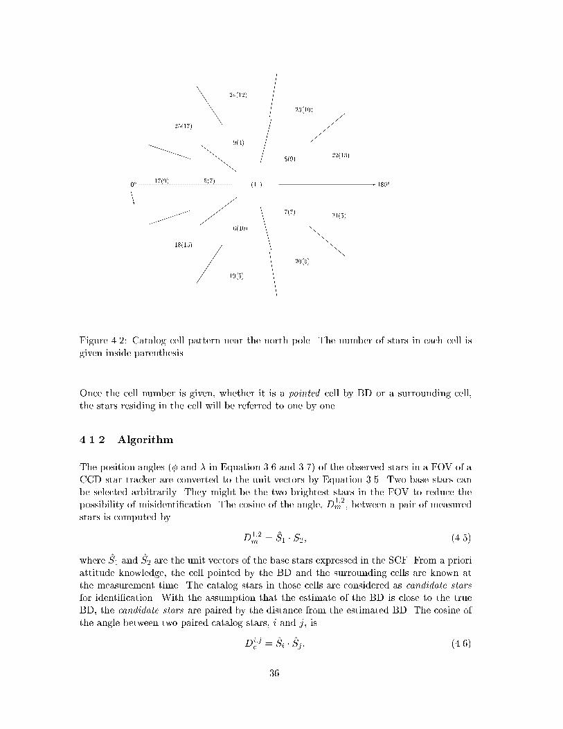
the star coordinates. Figure 4.2 and 4.3 show the cells near the north pole region andthe south pole region, respectively. The number of stars in each cell is indicated withinparentheses. The numbering of the cells starts from the north pole and it continues to thesouth pole. This alternative numbering between north and south hemispheres continuesuntil it arrives at the celestial equator zone which contains 45 equally spaced cells with allthe centers located at 2� declination. The maximum number of stars in a cell turns outto be 37, which occurs once. Three cells contain one star in a cell, however, there is nocell that has no stars. As we mentioned earlier in Section 3.3, either cells with excessivenumber of stars or with too few stars make the star identi�cation troublesome and maydegrade the accuracy of the attitude determination. It might be possible to develop morecomplicated codes to deal with dense and sparse regions with di�erent criteria.

To access the desired cells with the knowledge of the estimated BD (in � and �), thelocation of the cell is determined by a pointer, n2 + j, where n and j are obtained from[46]

n = 2[(�

2� �)=�� + 0:5] (� > 0�)

= 2N + 1� 2[(�

2� �)=�� + 0:5] (� < 0�) (4.3)

j = [�=�� + 0:5]; (4.4)

where �� and �� are the width of each cell in � and �. The symbol [ ] indicates thesmallest integer greater than (or equal to) the number inside.

To access the surrounding cells, we need to tabulate the numbers of surrounding cells foreach cell number. Figure 4.1 shows the surrounding cells around a cell pointed by the BD.

35

.

..

.

.

.

..

.

.

.

..

.

.

.

.

..

.

.

..

.

..

.

.

..

.

..

.

..

.

.

..

..

..

..

..

..

..

..

..

..

..

..

..

..

..

.

..

..

.

..

..

.

..

..

......................................................................

.............................................................................................................................................................................................................................................................................................................................................................

..........................................................................................................................................................

.

..

.

.

.

..

.

.

.

..

.

.

.

.

..

.

.

.

..

.

.

.

.

..

.

.

..

.

.

..

.

.

.

..

.

.

..

.

.

..

.

.

..

.

.

..

.

.

..

.

.

..

.

..

.

..

.

.

..

.

..

.

.

..

.

..

.

.

..

.

..

.

..

.

..

..

.

..

.

..

.

..

.

..

.

..

.

..

.

..

..

..

.

..

..

..

..

.

..

..

..

..

..

.

..

..

..

..

..

.

..

..

.

..

..

.

..

..

.

..

..

.

..

.

..

..

.

..

..

..

..

.

..

..

..

..

..

..

..

..

..

..

..

..

..

..

..

..

..

..

..

..

..

.

..

..

..

..

.................................................................................................................................................................................................

...............

.........................

.............................................................................................................................................................................................................................................................................................

..................................................................................................................................................................................................................................................................................................................................................................................................................................................................................................................................................................................................................................................................................................................................................................

.................................................................................................................................................................................................................................................................................................................................................................................................................................................................................................

.

..

.

.

.

..

.

.

.

..

.

.

.

..

.

.

.

..

.

.

.

..

.

.

.

..

.

.

.

..

.

.

.

..

.

.

..

.

.

..

.

.

..

.

.

..

.

.

.

..

.

.

..

.

.

..

.

.

..

.

.

..

.

.

..

.

.

..

.

..

.

.

..

.

..

.

.

..

.

..

.

.

..

.

..

.

.

..

.

.

..

.

..

.

..

.

..

.

..

.

..

.

.

..

.

..

.

..

.

..

.

..

.

..

.

..

.

..

.

..

.

..

.

..

.

..

..

.

..

.

..

..

.

..

.

..

.

..

..

.

..

.

..

..

.

..

.

..

..

..

.

..

..

..

..

..

.

..

..

..

..

.

..

..

..

..

..

.

..

..

..

..

..

.

..

..

..

.

..

..

..

.

..

..

..

.

..

..

..

.

..

..

..

.

..

.

..

.

..

.

..

.

..

..

..

.

..

.

..

.

..

..

..

.

..

.

..

.

..

..

..

..

.

..

..

.

..

..

..

..

..

.

..

..

.

..

..

..

..

..

.

..

..

..

..

.

..

..

..

..

..

..

..

.

..

..

..

..

..

..

..

.

..

..

..

..

..

..

..

..

..

..

..

......................................................................................................................................................................................................................................................................................................

...........

..................

..................

...................

..................................................................................................................................................................................................................................................................................................................................................................................................................................................................................

..................................

............................................................................................................................................................................................................................................................................................................................................................................................................................................................................................................................................................................................................................................................................................................................................................................................................................................................................................................................................................................................................................................................................................................................................................................................................................................................................

......................................................................................................................................................................................................................................................................................................................................................................................................................................................................................................................................................................................................................................................................................................................................................................................................................................-1(11)0� 180�

CCCW

�������

ZZ

ZZ

ZZ

��

��

��

CCCCCCC

8(9)

9(4)

5(7)

6(10)

7(7)

,,,,,,

�������

JJ

JJJJ

PPPP

PPP

�������

EEEEEEE

llllll

22(13)

23(10)

24(12)

25(17)

17(9)

18(15)

19(5)

20(6)

21(5)

Figure 4.2: Catalog cell pattern near the north pole. The number of stars in each cell isgiven inside parenthesis.

Once the cell number is given, whether it is a pointed cell by BD or a surrounding cell,the stars residing in the cell will be referred to one by one.

4.1.2 Algorithm

The position angles (� and � in Equation 3.6 and 3.7) of the observed stars in a FOV of aCCD star tracker are converted to the unit vectors by Equation 3.5. Two base stars canbe selected arbitrarily. They might be the two brightest stars in the FOV to reduce thepossibility of misidenti�cation. The cosine of the angle, D1;2

m , between a pair of measuredstars is computed by

D1;2m = S1 � S2; (4.5)

where S1 and S2 are the unit vectors of the base stars expressed in the SCF. From a prioriattitude knowledge, the cell pointed by the BD and the surrounding cells are known atthe measurement time. The catalog stars in those cells are considered as candidate starsfor identi�cation. With the assumption that the estimate of the BD is close to the trueBD, the candidate stars are paired by the distance from the estimated BD. The cosine ofthe angle between two paired catalog stars, i and j, is

Di;jc = Si � Sj ; (4.6)

36

..

.

.

.

..

.

.

.

..

.

.

.

..

.

.

.

..

.

.

.

..

.

.

..

.

..

.

.

..

.

.

..

.

..

.

.

..

.

.

..

.

..

.

..

.

..

.

..

..

.

..

.

..

.

..

.

..

.

..

..

..

..

..

.

..

..

..

..

..

..

..

..

..

..

.

..

.

..

.

..

.

..

.

..

.

..

..

..

.

..

.

..

..

..

..

.

..

..

..

..

..

..

..

..

.

..

..

............................................................................................................................

.......................

.......................................................................................................................................................................................

.....................

.........................................................................................................................................................................................................................................................................................................................................................................................................................................................................................................

.................................................................................................................................................................................................................................................................................................................................

.

..

.

.

.

..

.

.

.

..

.

.

.

..

.

.

.

..

.

.

.

.

..

.

.

.

..

.

.

..

.

.

..

.

.

.

..

.

.

..

.

.

..

.

.

.

..

.

.

..

.

.

..

.

..

.

.

..

.

.

..

.

..

.

.

..

.

..

.

.

..

.

.

..

.

..

.

..

.

..

.

.

..

.

..

.

..

.

..

.

..

.

..

.

..

.

..

.

..

.

..

.

..

.

..

..

.

..

.

..

.

..

..

.

..

.

..

.

..

..

..

.

..

..

..

..

.

..

..

..

..

.

..

..

..

..

.

..

..

.

..

..

..

.

..

..

..

.

..

..

..

.

..

..

..

.

..

..

.

..

.

..

..

..

.

..

.

..

.

..

..

..

.

..

.

..

.

..

..

.

..

..

..

..

..

.

..

..

.

..

..

..

..

..

.

..

..

..

..

..

..

..

..

..

..

..

..

..

.

..

..

..

..

................................................................................................................................................................................................................................................................................

..................

.....................................

............................................................................................................................................................................................................................................................................................................................................................................

...............................................................................................................................................................................................................................................................................................................................................................................................................................................................................................................................................................................................................................................................................................................................................................................................................................................................................................................................................................................................................................

...................................................................................................................................................................................................................................................................................................................................................................................................................................................................................................................................................................................................................................................................

.

..

.

.

.

..

.

.

.

..

.

.

.

.

..

.

.

.

..

.

.

.

..

.

.

.

.

..

.

.

.

..

.

.

.

..

.

.

..

.

.

.

..

.

.

..

.

.

.

..

.

.

..

.

.

.

..

.

.

..

.

.

.

..

.

.

..

.

.

..

.

.

..

.

..

.

.

..

.

.

..

.

.

..

.

.

..

.

.

..

.

.

..

.

..

.

.

..

.

..

.

.

..

.

..

.

.

..

.

..

.

..

.

.

..

.

..

.

.

..

.

..

.

..

.

..

.

..

.

..

.

.

..

.

..

.

..

.

..

.

..

.

..

.

..

.

..

.

..

.

..

.

..

.

..

..

.

..

.

..

..

.

..

.

..

.

..

..

.

..

.

..

.

..

..

.

..

.

..

..

.

..

..

..

..

.

..

..

..

.

..

..

..

..

.

..

..

..

.

..

..

..

..

..

..

..

..

..

..

.

..

..

..

..

..

..

.

..

..

..

..

..

..

..

.

..

.

..

..

.

..

.

..

.

..

..

.

..

.

..

.

..

.

..

..

.

..

.

..

.

..

.

..

..

..

..

..

.

..

..

..

..

..

..

..

..

..

..

..

.

..

..

..

..

..

..

..

..

..

..

..

.

..

..

..

..

..

..

..

..

..

..

..

..

..

..

..

..

..

..

..

..

..

..

.

..

..

..

..

..

..

..

..

..

..

..

..

..

..

..

..

.............................................................................................................................................................................................................................................................................................................................................................................

.............

.............

..............

.....................

............................

.............................................................................................................................................................................................................................................................................................................................................................................................................................................................................................................................................................

.................................

........................................................................................................................................................................................................................................................................................................................................................................................................................................................................................................................................................................................................................................................................................................................................................................................................................................................................................................................................................................................................................................................................................................................................................................................................................................................................................................................................................................................................................................................................................................................................

........................................................................................................................................................................................................................................................................................................................................................................................................................................................................................................................................................................................................................................................................................................................................................................................................................................................................................................................................................................................................-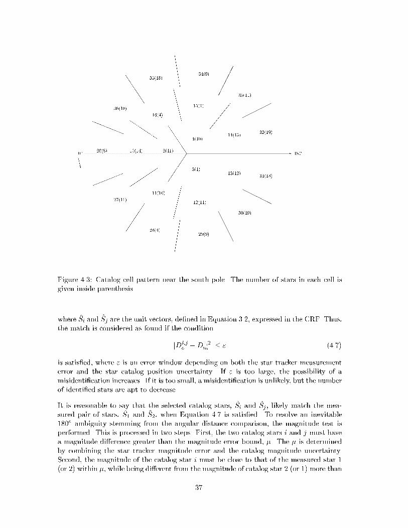J

JJ

JJJ

4(10)

2(11)

3(1)

0� 180�

CCCW

������

CCCCCCC

QQ

QQ

QQ

��

��

��

�������

\\\\\\

14(13)

15(9)

16(4)

10(14)

11(10)

12(11)

13(12)

����

���

�������

EEEEEEE

JJJ

JJJ

aaaa

aaa

!!!!!!!

�������

AAAAAAA

HHHHHHH

32(19)

33(11)

34(9)35(18)

36(10)

26(8)

27(11)

28(4)29(9)

30(19)

31(13)

Figure 4.3: Catalog cell pattern near the south pole. The number of stars in each cell isgiven inside parenthesis.

where Si and Sj are the unit vectors, de�ned in Equation 3.2, expressed in the CRF. Thus,the match is considered as found if the condition

jDi;jc �D1;2

m j � " (4.7)

is satis�ed, where " is an error window depending on both the star tracker measurementerror and the star catalog position uncertainty. If " is too large, the possibility of amisidenti�cation increases. If it is too small, a misidenti�cation is unlikely, but the numberof identi�ed stars are apt to decrease.

It is reasonable to say that the selected catalog stars, Si and Sj, likely match the mea-sured pair of stars, S1 and S2, when Equation 4.7 is satis�ed. To resolve an inevitable180� ambiguity stemming from the angular distance comparison, the magnitude test isperformed. This is processed in two steps. First, the two catalog stars i and j must havea magnitude di�erence greater than the magnitude error bound, �. The � is determinedby combining the star tracker magnitude error and the catalog magnitude uncertainty.Second, the magnitude of the catalog star i must be close to that of the measured star 1(or 2) within �, while being di�erent from the magnitude of catalog star 2 (or 1) more than

37

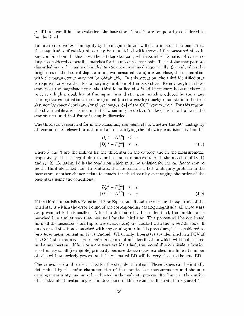
�. If these conditions are satis�ed, the base stars, 1 and 2, are temporarily considered tobe identi�ed.

Failure to resolve 180� ambiguity by the magnitude test will occur in two situations. First,the magnitudes of catalog stars may be unmatched with those of the measured stars inany combination. In this case, the catalog star pair, which satis�ed Equation 4.7, are nolonger considered as possible matches for the measured star pair. The catalog star pair arediscarded and other pairs of candidate stars are examined sequentially. Second, when thebrightness of the two catalog stars (or two measured stars) are too close, their separationwith the parameter � may not be obtainable. In this situation, the third identi�ed staris required to solve the 180� ambiguity problem of the base stars. Even though the basestars pass the magnitude test, the third identi�ed star is still necessary because there isrelatively high probability of �nding an invalid star pair match produced by too manycatalog star combinations, the unregistered (on star catalog) background stars in the truesky, nearby space debris and/or ghost images [54] of the CCD star tracker. For this reason,the star identi�cation is not initiated when only two stars (or less) are in a frame of thestar tracker, and that frame is simply discarded.

The third star is searched for in the remaining candidate stars, whether the 180� ambiguityof base stars are cleared or not, until a star satisfying the following conditions is found :

jDi;kc �D1;3

m j � "

jDj;kc �D2;3

m j � "; (4.8)

where k and 3 are the indices for the third star in the catalog and in the measurement,respectively. If the magnitude test for base stars is successful with the matches of (i; 1)and (j; 2), Equation 4.8 is the condition which must be satis�ed for the candidate star tobe the third identi�ed star. In contrast, if there remains a 180� ambiguity problem in thebase stars, another chance exists to match the third star by exchanging the order of thebase stars using the conditions :

jDi;kc �D2;3

m j � "

jDj;kc �D1;3

m j � ": (4.9)

If the third star satis�es Equation 4.8 or Equation 4.9 and the measured magnitude of thethird star is within the error bound of the corresponding catalog magnitude, all three starsare presumed to be identi�ed. After the third star has been identi�ed, the fourth star ismatched in a similar way that was used for the third star. This process will be continueduntil all the measured stars (up to �ve or six stars) are checked with the candidate stars. Ifan observed star is not matched with any catalog star in this procedure, it is considered tobe a false measurement and it is ignored. When only three stars are identi�ed in a FOV ofthe CCD star tracker, there remains a chance of misidenti�cation which will be discussedin the next section. If four or more stars are identi�ed, the probability of misidenti�cationis extremely small (negligible) primarily because the stars are searched in a limited numberof cells with an orderly process and the estimated BD will be very close to the true BD.

The values for " and � are critical for the star identi�cation. Those values can be initiallydetermined by the noise characteristics of the star tracker measurements and the starcatalog uncertainty, and must be adjusted in the real data process after launch. The outlineof the star identi�cation algorithm developed in this section is illustrated in Figure 4.4.

38

���

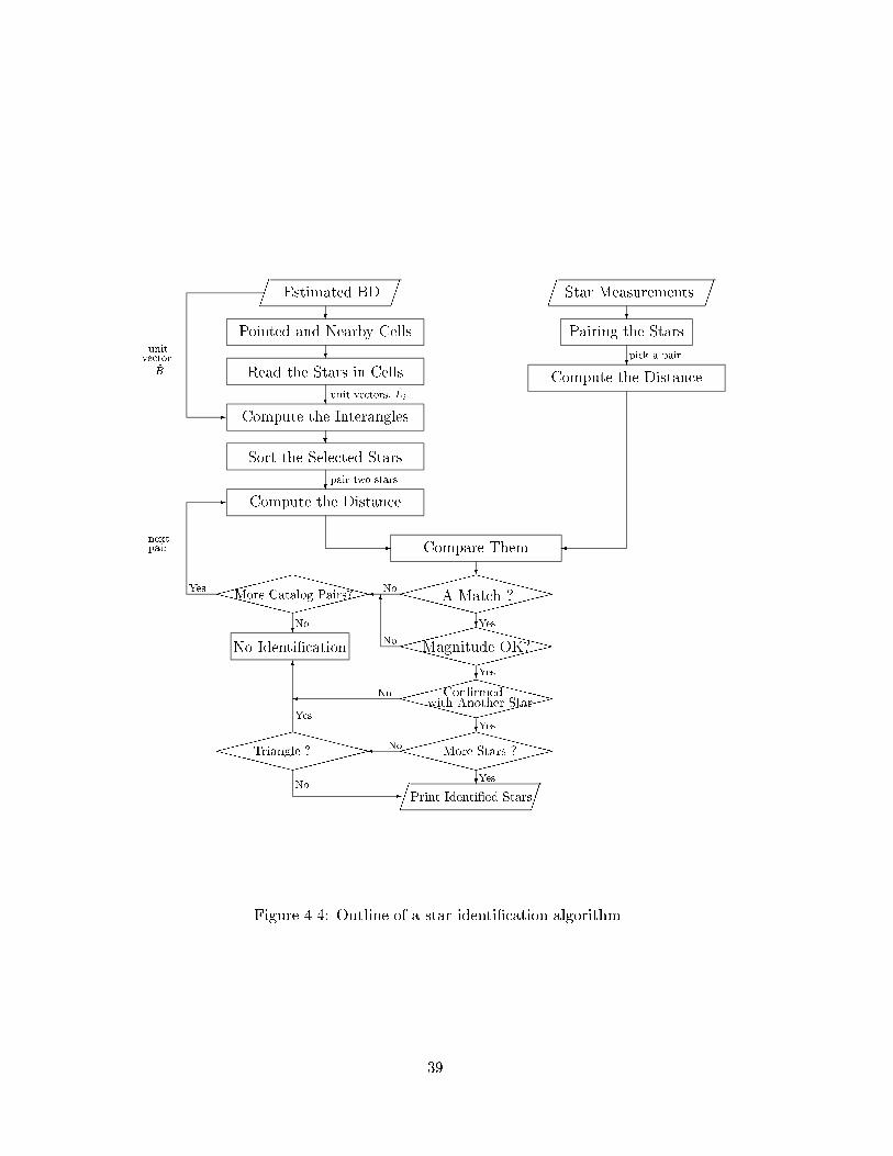
���Estimated BD

?Pointed and Nearby Cells

?Read the Stars in Cells

?unit vectors, Li

Compute the Interangles-

unitvector

B

?Sort the Selected Stars

?pair two stars

Compute the Distance

-

���

���Star Measurements

?Pairing the Stars

?pick a pair

Compute the Distance

�Compare Them

?

������XXXXXXXXXXXX���

���A Match ?No

?Yes

������XXXXXXXXXXXX���

���Magnitude OK?No

6

?Yes

�������XXXXXXXXXXXX���

���More Catalog Pairs?Yes

?No

No Identi�cation

-

nextpair

������XXXXXXXXXXXX���

���Con�rmed

with Another Star� No

?Yes

������XXXXXXXXXXXX���

���More Stars ?

?Yes

���

���Print Identi�ed Stars

� No������XXXXXXXXXXXX���

���Triangle ?

6

Yes

No-

Figure 4.4: Outline of a star identi�cation algorithm

39

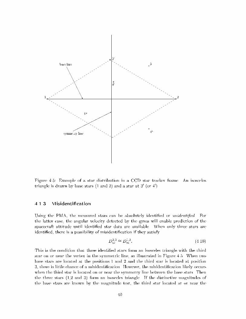
*1

*2

*3

*4

*40

*30

*400

*

..

..

..

..

..

..

.

..

..

..

..

..

..

..

..

..

.

..

..

..

..

..

..

..

..

..

.

..

..

..

..

..

..

..

..

..

..

..

..

.

..

..

..

..

..

..

..

..

..

.

..

..

..

..

..

..

..

..

..

.

..

..

..

..

..

..

..

..

..

.

..

..

..

..

..

..

..

..

..

.

..

..

..

..

..

..

..

..

..

.

..

..

..

..

..

..

..

..

..

.

..

..

..

..

..

..

..

..

..

..

..

..

.

..

..

..

..

..

..

..

..

..

.

..

..

..

..

..

..

..

..

..

.

..

..

..

..

..

..

..

..

..

.

..

..

..

..

..

..

..

..

..

.

..

..

..

..

..

..

..

..

..

.

..

..

..

..

..

..

..

..

..

.

..

..

..

..

..

..

..

..

..

..

..

..

.

..

..

..

..

..

..

..

..

..

.

..

..

..

..

..

..

..

..

..

.

..

..

..

..

..

..

..

..

..

.

..

..

..

..

..

..

..

..

..

.

..

..

..

..

..

..

..

..

..

.

..

..

..

..

..

..

..

..

..

.

..

..

..

..

..

..

..

..

..

..

..

..

.

..

..

..

..

..

..

..

..

..

.

..

..

..

..

..

..

..

..

..

.

..

..

..

..

..

..

..

..

..

.

..

..

..

..

..

..

..

..

..

.

..

..

..

..

..

..

..

..

..

.

..

..

..

..

..

..

..

..

..

.

..

..

..

..

..

..

..

..

..

..

..

..

.

..

..

..

..

..

..

..

..

..

.

..

..

..

..

..

..

..

..

..

.

..

..

..

..

..

..

..

..

..

.

..

..

..

..

..

..

..

..

..

.

..

..

..

..

..

..

..

..

..

.

..

..

..

..

..

..

..

..

..

.

..

..

..

..

..

..

..

..

..

.

..

..

..

..

..

..

..

..

..

..

..

..

.

..

..

..

..

..

..

..

..

..

.

..

..

..

..

..

..

..

..

..

.

..

..

..

..

..

..

..

..

..

.

..

..

..

..

..

..

..

..

..

.

..

..

..

..

..

..

..

..

..

.

..

..

..

..

..

..

..

..

.

..

..

..

..

..

..

..

..

..

..

..

..

..

.

..

..

..

..

..

..

..

..

..

.

..

..

..

..

..

..

..

..

..

.

..

..

..

..

..

..

..

..

..

.

..

..

..

..

..

..

..

..

..

.

..

..

..

..

..

..

..

..

..

.

..

..

..

..

..

..

..

..

..

.

..

..

..

..

..

..

..

..

..

..

..

..

.

..

..

..

..

..

..

..

..

..

.

..

..

..

..

..

..

..

..

..

.

..

..

..

..

..

..

..

..

..

.

..

..

..

..

..

..

..

..

..

.

..

..

..

..

..

..

..

..

..

.

..

..

..

..

..

..

..

..

..

.

..

..

..

..

..

..

..

..

..

..

..

..

.

..

..

..

..

..

..

..

..

..

.

..

..

..

..

..

..

..

..

..

.

..

..

..

..

..

..

..

..

..

.

..

..

..

..

..

..

..

..

..

.

..

..

..

..

..

..

..

..

..

.

..

..

..

..

..

..

..

..

..

.

..

..

..

..

..

..

..

..

..

..

..

..

.

..

..

..

..

..

..

..

..

..

.

..

..

..

..

..

..

..

..

..

.

..

..

..

..

..

..

..

..

..

.

..

..

..

..

..

..

..

..

..

.

.

..

..

.

..

..

..

.

..

..

..

..

..

..

..

.

..

..

..

.

..

..

..

.

..

..

..

.

..

..

..

.

..

..

..

.

..

..

..

.

..

..

..

.

..

..

..

.

..

..

..

.

..

..

..

.

..

..

..

.

..

..

..

.

..

..

..

.

..

..

..

.

..

..

..

.

..

..

..

.

..

..

..

.

..

..

..

.

..

..

..

.

..

..

..

.

..

..

..

.

..

..

..

.

..

..

..

.

..

..

..

.

..

..

..

.

..

..

..

.

..

..

..

.

..

..

..

.

..

..

..

.

..

..

..

.

..

..

..

.

..

..

..

.

..

..

..

.

..

..

..

.

..

..

..

.

..

..

..

.

..

..

..

.

..

..

..

.

..

..

..

.

..

..

..

.

..

..

..

.

..

..

..

.

..

..

..

.

..

..

..

.

..

..

..

.

..

..

..

.

..

..

..

..

..

..

..

.

..

..

..

.

..

..

..

.

..

..

..

.

..

..

..

.

..

..

..

.

..

..

..

.

..

..

..

.

..

..

..

.

..

..

..

.

..

..

..

.

..

..

..

.

..

..

..

.

..

..

..

.

..

..

..

.

..

..

..

.

..

..

..

.

..

..

..

.

..

..

..

.

..

..

..

.

..

..

..

.

..

..

..

.

..

..

..

.

..

..

..

.

..

..

..

.

..

..

..

.

..

..

..

.

..

..

..

.

..

..

..

.

..

..

..

.

..

..

..

.

..

..

..

.

..

..

..

.

..

..

..

.

..

..

..

.

..

..

..

.

..

..

..

.

..

..

..

.

..

..

..

.

..

..

..

.

..

..

..

.

..

..

..

.

..

..

..

.

..

..

..

.

..

..

..

.

..

..

..

.

..

..

..

.

..

..

..

.

..

..

..

..

..

..

..

.

..

..

..

.

..

..

..

.

..

..

..

.

..

..

..

.

..

..

..

.

..

..

..

.

..

..

..

.

..

..

..

.

..

..

..

.

..

..

..

.

..

..

..

.

..

..

..

.

..

..

..

.

..

..

.

..

..

..

.

..

..

..

..

.

..

..

..

.

..

..

..

.

..

..

..

.

..

..

..

.

..

..

..

.

..

..

..

.

..

..

..

.

..

..

..

.

..

..

..

.

..

..

..

.

..

..

..

.

..

..

..

.

..

..

..

.

..

..

..

.

..

..

..

.

..

..

..

.

..

..

..

.

..

..

..

.

..

..

..

.

..

..

..

.

..

..

..

.

..

..

..

.

..

..

..

.

..

..

..

.

..

..

..

.

..

..

..

.

..

..

..

.

..

..

..

.

..

..

..

.

..

..

..

.

..

..

..

..

..

..

..

.

..

..

..

.

..

..

..

.

..

..

..

.

..

..

..

.

..

..

..

.

..

..

..

.

..

..

..

.

..

..

..

.

..

..

..

.

..

..

..

.

..

..

..

.

..

..

..

.

..

..

..

.

..

..

..

.

..

..

..

.

..

..

..

.

..

..

..

.

..

..

..

.

..

..

..

.

..

..

..

.

..

..

..

.

..

..

..

.

..

..

..

.

..

..

..

.

..

..

..

.

..

..

..

.

..

..

..

..

..

..

.

..

..

..

..

..

..

..

..

..

.

..

..

..

..

..

..

..

..

..

.

..

..

..

..

..

..

..

..

..

..

..

..

.

..

..

..

..

..

..

..

..

..

.

..

..

..

..

..

..

..

..

..

.

..

..

..

..

..

..

..

..

..

.

..

..

..

..

..

..

..

..

..

.

..

..

..

..

..

..

..

..

..

.

..

..

..

..

..

..

..

..

..

.

..

..

..

..

..

..

..

..

..

..

..

..

.

..

..

..

..

..

..

..

..

..

.

..

..

..

..

..

..

..

..

..

.

..

..

..

..

..

..

..

..

..

.

..

..

..

..

..

..

..

..

..

.

..

..

..

..

..

..

..

..

..

.

..

..

..

..

..

..

..

..

..

.

..

..

..

..

..

..

..

..

..

..

..

..

.

..

..

..

..

..

..

..

..

..

.

..

..

..

..

..

..

..

..

..

.

..

..

..

..

..

..

..

..

..

.

..

..

..

..

..

..

..

..

..

.

..

..

..

..

..

..

..

..

..

.

..

..

..

..

..

..

..

..

..

.

..

..

..

..

..

..

..

..

..

..

..

..

.

..

..

..

..

..

..

..

..

..

.

..

..

..

..

..

..

..

..

..

.

..

..

..

..

..

..

..

..

..

.

..

..

..

..

..

..

..

..

..

.

..

..

..

..

..

..

..

..

..

.

..

..

..

..

..

..

..

..

..

.

..

..

..

..

..

..

..

..

..

..

..

..

.

..

..

..

..

..

..

..

..

..

.

..

..

..

..

..

..

..

..

..

.

..

..

..

..

..

..

..

..

..

.

..

..

..

..

..

..

..

..

..

.

..

..

..

..

..

..

..

..

..

.

..

..

..

..

..

..

..

..

..

.

..

..

..

..

..

..

..

..

..

.

..

..

..

..

..

..

..

..

..

..

..

..

.

..

..

..

..

..

..

..

..

..

.

..

..

..

..

..

..

..

..

..

.

..

..

..

..

..

..

..

..

..

.

..

..

..

..

..

..

..

..

..

.

..

..

..

..

..

..

..

..

..

.

..

..

..

..

..

..

..

..

.

..

..

..

..

..

..

..

..

..

..

..

..

..

.

..

..

..

..

..

..

..

..

..

.

..

..

..

..

..

..

..

..

..

.

..

..

..

..

..

..

..

..

..

.

..

..

..

..

..

..

..

..

..

.

..

..

..

..

..

..

..

..

..

.

..

..

..

..

..

..

..

..

..

.

..

..

..

..

..

..

..

..

..

..

..

..

.

..

..

..

..

..

..

..

..

..

.

..

..

..

..

..

..

..

..

..

.

..

..

..

..

..

..

..

..

..

.

..

..

..

..

..

..

..

..

..

.

..

..

..

..

..

..

..

..

..

.

..

..

..

..

..

..

..

..

..

.

..

..

..

..

..

..

..

..

..

..

..

..

.

..

..

..

..

..

..

..

..

..

.

..

..

..

..

..

..

..

..

..

.

..

..

..

..

..

..

..

..

..

.

..

..

..

..

..

..

..

..

..

.

..

..

..

..

..

..

..

..

..

.

..

..

..

..

..

..

..

..

..

.

..

..

..

..

..

..

..

..

..

..

..

..

.

..

..

..

..

..

..

..

..

..

.

..

..

..

..

..

..

..

..

..

.

..

..

..

..

..

..

..

..

..

.

..

..

..

..

..

..

..

..

..

.

.

..

..

.

..

..

..

.

..

..

..

..

..

..

..

.

..

..

..

.

..

..

..

.

..

..

..

.

..

..

..

.

..

..

..

.

..

..

..

.

..

..

..

.

..

..

..

.

..

..

..

.

..

..

..

.

..

..

..

.

..

..

..

.

..

..

..

.

..

..

..

.

..

..

..

.

..

..

..

.

..

..

..

.

..

..

..

.

..

..

..

.

..

..

..

.

..

..

..

.

..

..

..

.

..

..

..

.

..

..

..

.

..

..

..

.

..

..

..

.

..

..

..

.

..

..

..

.

..

..

..

.

..

..

..

.

..

..

..

.

..

..

..

.

..

..

..

.

..

..

..

.

..

..

..

.

..

..

..

.

..

..

..

.

..

..

..

.

..

..

..

.

..

..

..

.

..

..

..

.

..

..

..

.

..

..

..

.

..

..

..

.

..

..

..

.

..

..

..

.

..

..

..

..

..

..

..

.

..

..

..

.

..

..

..

.

..

..

..

.

..

..

..

.

..

..

..

.

..

..

..

.

..

..

..

.

..

..

..

.

..

..

..

.

..

..

..

.

..

..

..

.

..

..

..

.

..

..

..

.

..

..

..

.

..

..

..

.

..

..

..

.

..

..

..

.

..

..

..

.

..

..

..

.

..

..

..

.

..

..

..

.

..

..

..

.

..

..

..

.

..

..

..

.

..

..

..

.

..

..

..

.

..

..

..

.

..

..

..

.

..

..

..

.

..

..

..

.

..

..

..

.

..

..

..

.

..

..

..

.

..

..

..

.

..

..

..

.

..

..

..

.

..

..

..

.

..

..

..

.

..

..

..

.

..

..

..

.

..

..

..

.

..

..

..

.

..

..

..

.

..

..

..

.

..

..

..

.

..

..

..

.

..

..

..

.

..

..

..

..

..

..

..

.

..

..

..

.

..

..

..

.

..

..

..

.

..

..

..

.

..

..

..

.

..

..

..

.

..

..

..

.

..

..

..

.

..

..

..

.

..

..

..

.

..

..

..

.

..

..

..

.

..

..

..

.

..

..

.

..

..

..

.

..

..

..

..

.

..

..

..

.

..

..

..

.

..

..

..

.

..

..

..

.

..

..

..

.

..

..

..

.

..

..

..

.

..

..

..

.

..

..

..

.

..

..

..

.

..

..

..

.

..

..

..

.

..

..

..

.

..

..

..

.

..

..

..

.

..

..

..

.

..

..

..

.

..

..

..

.

..

..

..

.

..

..

..

.

..

..

..

.

..

..

..

.

..

..

..

.

..

..

..

.

..

..

..

.

..

..

..

.

..

..

..

.

..

..

..

.

..

..

..

.

..

..

..

.

..

..

..

..

..

..

..

.

..

..

..

.

..

..

..

.

..

..

..

.

..

..

..

.

..

..

..

.

..

..

..

.

..

..

..

.

..

..

..

.

..

..

..

.

..

..

..

.

..

..

..

.

..

..

..

.

..

..

..

.

..

..

..

.

..

..

..

.

..

..

..

.

..

..

..

.

..

..

..

.

..

..

..

.

..

..

..

.

..

..

..

.

..

..

..

.

..

..

..

.

..

..

..

.

..

..

..

.

..

..

..

.

AAAAAAAAAAU

base line

����

����

����*

symmetry line

Figure 4.5: Example of a star distribution in a CCD star tracker frame. An isoscelestriangle is drawn by base stars (1 and 2) and a star at 30 (or 40).

4.1.3 Misidenti�cation

Using the PMA, the measured stars can be absolutely identi�ed or unidenti�ed. Forthe latter case, the angular velocity detected by the gyros will enable prediction of thespacecraft attitude until identi�ed star data are available. When only three stars areidenti�ed, there is a possibility of misidenti�cation if they satisfy

D2;3m�= D1;3

m : (4.10)

This is the condition that three identi�ed stars form an isosceles triangle with the thirdstar on or near the vertex in the symmetric line, as illustrated in Figure 4.5. When twobase stars are located at the positions 1 and 2 and the third star is located at position3, there is little chance of a misidenti�cation. However, the misidenti�cation likely occurswhen the third star is located on or near the symmetry line between the base stars. Thenthe three stars (1,2 and 3) form an isosceles triangle. If the distinctive magnitudes ofthe base stars are known by the magnitude test, the third star located at or near the

40

symmetry line provides more con�dence on the correct identi�cation of the base stars.However, as long as the 180� ambiguity of the base stars is not resolved and if the thirdstar is located at or near the symmetry line, insu�cient information exists to distinguishthe base stars. That measurement frame is simply discarded and rendered as unidenti�edat the expense of the loss of the possible correct matches. Since it is not likely to have two(for example, 30 and 40 in Figure 4.5) or more stars located on or near the symmetry line,the case of only three identi�ed stars would need to be checked for the possible source ofthe misidenti�cation. Therefore, procedures to detect the isosceles triangle with a 180�

ambiguity must be added to the star identi�cation algorithm.

In addition to the isosceles triangle shape, there could be other special geometric con�gu-rations made by observed stars. For example, if there is a background star in position 400

(symmetric about the base line to the third star in position 3), it may be misidenti�ed as astar 3 regardless that the star (400) is a registered star in the star catalog or a simple back-ground star. We can imagine other special geometries formed by three, four or �ve starswhich require more sophisticated star identi�cation algorithms to avoid misidenti�cation.

There are other sources of misidenti�cation that originate from non-geometrical reasons.One example is space debris (or other satellites) near a star tracker BD. Since the startracker does not discern these sources from a real star, debris may cause misidenti�cation.(Debris actually caused a more serious problem in the star tracker performance of theX-ray Timing Explorer (XTE) spacecraft [9]). Ghost images of the CT-601 have beenreported as an identi�cation error source [54]. The star identi�cation algorithm must besu�ciently smart to consider ghost images as background stars that are unregistered inthe mission star catalog.

It is possible in the attitude estimation procedure to detect the measurement frame whichhas misidenti�ed stars. The abnormal discontinuity of quaternions (or the computed an-gular velocity) obtained by Single Frame Attitude Determination (SFAD) methods (Chap-ter 5) could be interpreted as an outbreak of the misidenti�cation. Even though we supposethat the PMA could include the detection of various misidenti�cation sources, the completeescape from the misidenti�cation would not be easy.

4.1.4 Simulation Results

The star tracker measurements were simulated for four circular orbits with 94� inclina-tion using the algorithm developed in Section 3.1. The respective initial positions are0�; 45�; 90� and 135� right ascensions at the equator. The time interval between succes-sive FOVs is 0.1 second. The measurement noises were computed based on the 1� valuesgiven in Section 3.1.3 for generating realistic simulation data.

The PMA was applied to the simulated star measurement data and the results are sum-marized in Table 4.1. In the simulation, the possible maximum number of FOVs for eachorbit is 57901 corresponding to a 10Hz measurement rate for one GLAS orbital period.Since the minimum number of stars necessary for the identi�cation process is three, thenumber of frames containing at least three stars are shown in the second column of Ta-ble 4.1. The � in the third column is a parameter representing the range in which the

41

third star is considered in a position to form an isosceles triangle with base stars. It iscomputed by

� = jD1;3m �D2;3

m j (4.11)

which means the distance di�erence between two sides of triangles other than the baseline. In other words, if the third star, 3, is located at a position to make the right sideof Equation 4.11 less than �, the three identi�ed stars are considered to form an isoscelestriangle. These stars are regarded as possible misidenti�cation cases and are abandoned.The identi�cation processing is resumed in order to �nd another group of stars which donot construct the isosceles triangle de�ned by Equation 4.11.

Table 4.1 shows that all the star tracker measurement frames are reported as identi�ed(indicated by 100%) if the isosceles triangle formed by the three stars is simply regardedas a correct identi�cation (� = 0). However, the misidenti�cation occurred in some framesas indicated in the last column of the Table 4.1, except for the case with 45� initial rightascension, �. For example, 0� initial � contains 167 misidenti�ed frames, which is 0:3% ofthe reported identi�ed frames. Computed results show that when the angle � is increased,the occurrence of the misidenti�cation is decreased and �nally disappears. There are morereductions in the total number of identi�ed frames (see the seventh column in Table 4.1)than the number of misidenti�ed ones (the eighth column). This clearly indicates thatthe elimination of the misidenti�cation source results in the removal of some correctlyidenti�ed frames. Table 4.1 also shows that the number of frames with �ve identi�edstars (the sixth column) increases as � increases. This means that the misidenti�cationin some frames hinders the determination of correct star matches. The lowest probabilityof successfully identifying stars without misidenti�cation was 98:59% in the simulation.Even though this result is undoubtedly promising, further star identi�cation tests (andnecessary improvements) should be carried out with more background stars in which themagnitude range covers up to eighth or ninth.

4.2 Direct Match Technique (DMT)

4.2.1 Algorithm

The requirement of more than two stars as well as the relatively high possibility of themisidenti�cation when only three stars are present in the star tracker FOV were pointedout as shortcomings of the PMA. The DMT enables us to identify the stars when the FOVcontains only one or two stars. Once the GLAS attitude determination is initialized anddetermines attitude in the required accuracy, the DMT can identify almost all stars ob-served by the FOV. The prediction of attitude can be achieved by applying the kinematicequation of attitude quaternions, Equation 2.11. Alternatively, the quaternions obtainedby the real time on-board attitude determination can be used. The accuracy requirementfor real time is 10-20 arcseconds(1�). Figure 4.6 illustrates the relations of the coordinateframes in the DMT. The star tracker observes up to six stars at a measurement time. Ifeither the predicted or the real time attitude is known, the star positions will be trans-formed from the SCF to the CRF (the observed CRF in Figure 4.6). If either the predicted

42

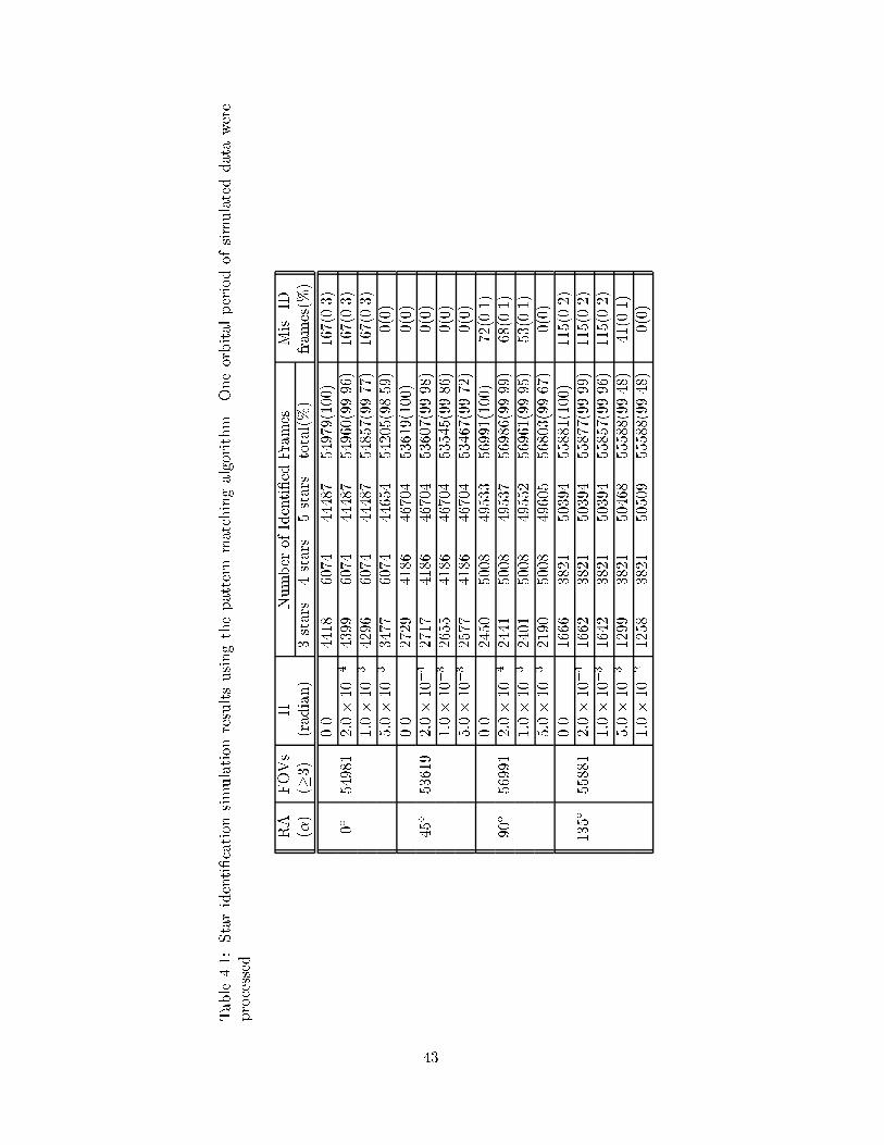
Table4.1:Staridenti�cationsimulationresultsusingthepatternmatchingalgorithm.Oneorbitalperiodofsimulateddatawere

processed.

RA

FOVs

�

NumberofIdenti�edFrames

Mis.ID

(�)

(�3)

(radian)

3stars

4stars

5stars

total(%)

frames(%)

0.0

4418

6074

44487

54979(100)

167(0.3)

0�

54981

2:0�10�4

4399

6074

44487

54960(99.96)

167(0.3)

1:0�10�3

4296

6074

44487

54857(99.77)

167(0.3)

5:0�10�3

3477

6074

44654

54205(98.59)

0(0)

0.0

2729

4186

46704

53619(100)

0(0)

45�

53619

2:0�10�4

2717

4186

46704

53607(99.98)

0(0)

1:0�10�3

2655

4186

46704

53545(99.86)

0(0)

5:0�10�3

2577

4186

46704

53467(99.72)

0(0)

0.0

2450

5008

49533

56991(100)

72(0.1)

90�

56991

2:0�10�4

2441

5008

49537

56986(99.99)

68(0.1)

1:0�10�3

2401

5008

49552

56961(99.95)

53(0.1)

5:0�10�3

2190

5008

49605

56803(99.67)

0(0)

0.0

1666

3821

50394

55881(100)

115(0.2)

135�

55881

2:0�10�4

1662

3821

50394

55877(99.99)

115(0.2)

1:0�10�3

1642

3821

50394

55857(99.96)

115(0.2)

5:0�10�3

1299

3821

50468

55588(99.48)

41(0.1)

1:0�10�2

1258

3821

50509

55588(99.48)

0(0)

43

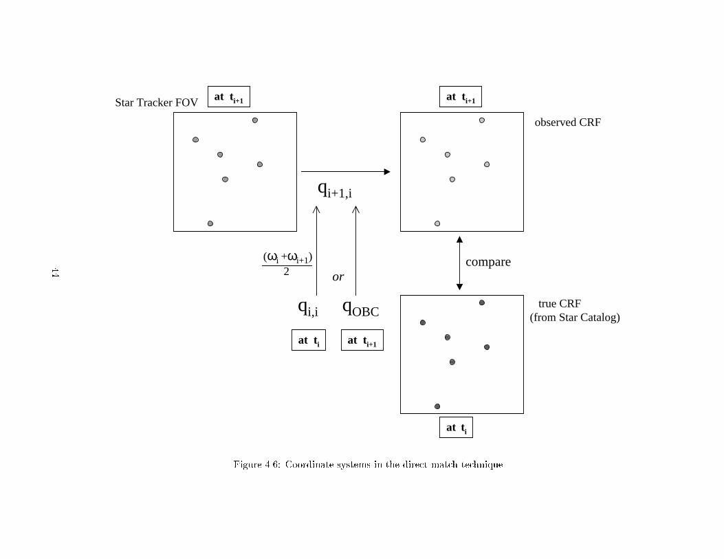
Star Tracker FOV

observed CRF

true CRF(from Star Catalog)

at ti+1 at ti+1

qi+1,i

qi,i

(ωi +ωi+1)

2

at ti

at ti

compare

qOBC

at ti+1

or

Figure 4.6: Coordinate systems in the direct match technique

44

observed star (O)catalog(true) star (S)

at ti

at ti+1

Vs/c

ε

Figure 4.7: Catalog stars close to measured stars

or the real time attitude is su�ciently close to the true attitude, the small circular areacentered by the observed star will be searched in the star catalog (Figure 4.7). By de�ning� as the error window radius of the circular area, the catalog star satisfying the equation

d(O; S) < � (4.12)

will be considered as the matched star, where d(O; S) is the angular distance between O,the observation unit vector in the observed CRF, and S, the catalog star unit vector inthe true CRF. The value for � is determined by the accuracy of the predicted or real timeattitude.

It is easy to see that the procedure described here would provide unique star identi�cationif the density of star population is considered. Since the HD-1003 star tracker will observestars brighter than magnitude 6, the number of stars in the corresponding star catalog isgenerally �ve or six thousand. In this case, the stellar density of the catalog is roughlyless than 1 star per square degree. By selecting several tens of arcseconds as the errorwindow radius, �, in Equation 4.12, we are able to identify almost all stars uniquely. Ifmultiple stars are found in the error window radius, additional work has to be done withthe comparison of either star magnitudes or the error sizes, d(O; S), in order to achieve

45

the unique identi�cation. If no star is found within the radius �, the observed star mightbe the non-star object or the predicted (or real time) attitude might have large error.

4.2.2 Catalog Star Search

In the PMA, the area to search for the matched star should be larger than the startracker FOV, 8� � 8�. It was required to divide the celestial sphere into many cells inorder to look at the restricted region in stead of the whole sky. (see Section 4.1.1). Inthe DMT, a star can be identi�ed by looking at the small circular area whose radius isusually tens of arcseconds with the observed star at the center. The method sectioningthe star catalog into many cells could be applied to the DMT, but the size of each cellmust be much smaller than that for the PMA in order to e�ciently search the area of theseveral tens of arcseconds � radius (Equation 4.12). This would require excessive work tocreate and organize more than several thousand cells and access to each cell in the searchprocess would be problematic when we consider the limited computation time. Therefore,the DMT developed for the GLAS PAD applies a new approach that does not use thesectioning of the star catalog described in Section 4.1.1. As the �rst step of the newapproach, the catalog stars whose right ascensions, �, are su�ciently close to the observedstars will be selected as candidate stars for identi�cation. Since the star tracker is ableto track the stars, the most probable matched star is the one that was identi�ed at theprevious measurement time. By looking at the catalog stars in both the increasing anddecreasing direction of catalog numbers, from previously identi�ed number, k, it is verylikely to �nd catalog stars whose right ascensions, �, are in several tens of arcseconds fromthat of the observed star, unless the star is new to the star tracker FOV. Therefore, thesearch area can be restricted to :

�0 � � < � < �0 + �; (4.13)

where �0 is the observed star � (see Figure 4.8(a)) and � is the error window radius alreadyintroduced in Equation 4.12.

For a star newly moving into the FOV (see the bottom of Figure 4.7), the � boundarydoesn't help �nd the match and we need to extend the search area. We refer to one ofthe previously identi�ed star catalog numbers and need to search � 8� right ascensionrange both in increasing and decreasing k directions (Figure 4.8(b)). To reduce the searchtime, we may further restrict the search area within � �4� right ascension range fromthe predicted BD. Equation 4.12 is applied to the stars residing in the selected � range inorder to choose the correct match for the observed star.

The search method described here performed well in the simulation. However, due tothe nature of the longitude and latitude system for the celestial sphere, a large numberof stars (sometimes all the stars in the star catalog) had to be looked at when the startracker observed the vicinity of the polar regions. This search method has been improvedby dividing the celestial sphere according to latitude zones as shown in Figure 4.9. Thiszoning of the star catalog is a reduced version of sectioning described in Section 4.1.1. Toavoid looking up to nearby zones, each zone is overlapped with the neighboring zones. Thiscould enable us to search only a rectangular area represented by thick lines in Figure 4.9(b)instead of the area indicated in 4.9(a).

46

+

RA(α)

α0+εα0α0-ε

k(catalog number)

decreasing

increasing

BD

∆α1

∆α1

∆α2

∆α2

∆α1 ≥ 4˚∆α2 ≥ 8˚

(a) for existing star (b) for new star

k

ε

ε

Figure 4.8: Search for matched star in star catalog

47

α0+∆αα0-∆α

α0+∆αα0-∆α

(a)

(b)

zone 1

zone 2

zone 3

zone 4

Dec

linat

ion

Dec

linat

ion

Right Ascension (α)

Right Ascension (α)

Figure 4.9: Searching area for star identi�cation. Latitude zones more than 4 are expected.

4.2.3 Simulation Results

In the simulation of the DMT, we achieved almost 100% successful star identi�cationswithout any misidenti�cation. Table 4.2 shows the results obtained by the DMT when thesame simulation data as for the PMA were used.

Table 4.2: Star identi�cation simulation results using the direct match technique. Oneorbital period of simulated data were processed.

RA Total Number of Number of Number of(�) Observed Stars Identi�ed Stars Misidenti�ed Stars

0� 265738 265735 (99.999%) 045� 265003 265003 (100.00%) 090� 276872 276867 (99.998%) 0135� 275330 275232 (99.964%) 0

48

Chapter 5

ATTITUDE DETERMINATION

5.1 Single Frame Attitude Determination

In this section, several algorithms will be introduced to determine the spacecraft attitudefrom the observed unit vectors. Since these algorithms determine attitude from measure-ment data obtained by a frame of a CCD star tracker, they will be called Single FrameAttitude Determination (SFAD) methods in this document.

Because the loss function J(A) in Wahba Problem (Equation 2.20) can be scaled withouta�ecting the optimum attitude matrix, Aopt, it is possible to normalize the weights suchas

nXi=1

ai = 1 (5.1)

with no loss of generality. Then the loss function can be easily manipulated to

J(A) = 1�nXi=1

aiWTi AVi

= 1� g(A): (5.2)

The loss function J(A) will have a minimum value when the gain function g(A) has amaximum value. The g(A) is given by

g(A) =nXi=1

aiWTi AVi

=

nXi=1

aitr[AViWTi ]

= tr[ABT ]; (5.3)

where tr means trace of a matrix and the B-matrix or Attitude Pro�le Matrix, B, is,

B =nXi=1

aiWiVTi : (5.4)

49

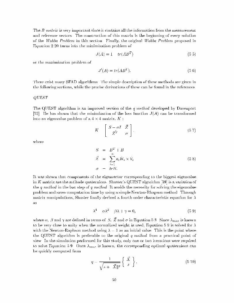
The B-matrix is very important since it contains all the information from the measurementand reference vectors. The construction of this matrix is the beginning of every solutionof the Wahba Problem in this section. Finally, the original Wahba Problem proposed inEquation 2.20 turns into the minimization problem of

J(A) = 1� tr(ABT ) (5.5)

or the maximization problem of

J 0(A) = tr(ABT ): (5.6)

There exist many SFAD algorithms. The simple description of these methods are given inthe following sections, while the precise derivations of these can be found in the references.

QUEST

The QUEST algorithm is an improved version of the q-method developed by Davenport[52]. He has shown that the minimization of the loss function J(A) can be transformedinto an eigenvalue problem of a 4� 4 matrix, K :

K =

"S � �I ~Z~ZT �

#: (5.7)

where

S = BT +B

~Z =

nXi=1

aiWi � Vi (5.8)

� = trB:

It was shown that components of the eigenvector corresponding to the biggest eigenvalueinK matrix are the attitude quaternions. Shuster's QUEST algorithm [39] is a variation ofthe q-method in the last step of q-method. It avoids the necessity for solving the eigenvalueproblem and saves computation time by using a simple Newton-Rhapson method. Throughmatrix manipulations, Shuster �nally derived a fourth order characteristic equation for �as

�4 � ��2 � ��+ = 0; (5.9)

where �; � and are de�ned in terms of S; ~Z and � in Equation 5.8. Since �max is knownto be very close to unity when the normalized weight is used, Equation 5.9 is solved for �with the Newton-Raphson method using � = 1 as an initial value. This is the point wherethe QUEST algorithm is preferable to the original q-method from a practical point ofview. In the simulation performed for this study, only one or two iterations were requiredto solve Equation 5.9. Once �max is known, the corresponding optimal quaternions canbe quickly computed from

q =1q

s+ k ~Xk2

�~Xs

�; (5.10)

50

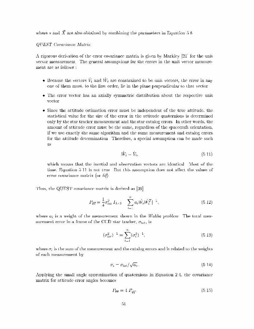
where s and ~X are also obtained by combining the parameters in Equation 5.8.

QUEST Covariance Matrix

A rigorous derivation of the error covariance matrix is given by Markley [21] for the unitvector measurement. The general assumptions for the errors in the unit vector measure-ment are as follows :

� Because the vectors Vi and Wi are constrained to be unit vectors, the error in anyone of them must, to the �rst order, lie in the plane perpendicular to that vector.

� The error vector has an axially symmetric distribution about the respective unitvector.

� Since the attitude estimation error must be independent of the true attitude, thestatistical value for the size of the error in the attitude quaternions is determinedonly by the star tracker measurement and the star catalog errors. In other words, theamount of attitude error must be the same, regardless of the spacecraft orientation,if we use exactly the same algorithm and the same measurement and catalog errorsfor the attitude determination. Therefore, a special assumption can be made suchas

Wi = Vi; (5.11)

which means that the inertial and observation vectors are identical. Most of thetime, Equation 5.11 is not true. But this assumption does not a�ect the values oferror covariance matrix (or �~q).

Thus, the QUEST covariance matrix is derived as [39]

P~q~q =1

4�2tot[I3�3 �

nXi=1

ai ~Wi~W Ti ]

�1; (5.12)

where ai is a weight of the measurement shown in the Wahba problem. The total mea-surement error in a frame of the CCD star tracker, �tot, is

(�2tot)�1 =

nXi=1

(�2i )�1; (5.13)

where �i is the sum of the measurement and the catalog errors and is related to the weightsof each measurement by

�i = �tot=pai: (5.14)

Applying the small angle approximation of quaternions in Equation 2.4, the covariancematrix for attitude error angles becomes

P�� = 4 P~q~q: (5.15)

51

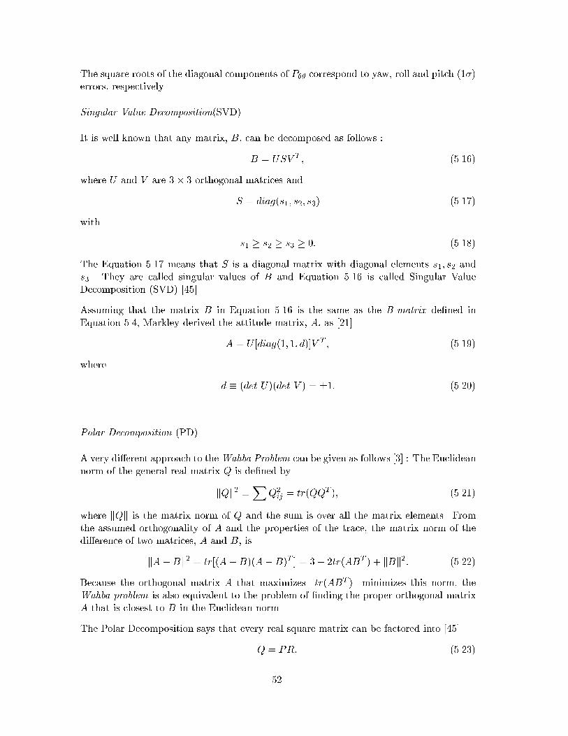
The square roots of the diagonal components of P�� correspond to yaw, roll and pitch (1�)errors, respectively.

Singular Value Decomposition(SVD)

It is well known that any matrix, B, can be decomposed as follows :

B = USV T ; (5.16)

where U and V are 3� 3 orthogonal matrices and

S = diag(s1; s2; s3) (5.17)

with

s1 � s2 � s3 � 0: (5.18)

The Equation 5.17 means that S is a diagonal matrix with diagonal elements s1; s2 ands3. They are called singular values of B and Equation 5.16 is called Singular ValueDecomposition (SVD) [45].

Assuming that the matrix B in Equation 5.16 is the same as the B-matrix de�ned inEquation 5.4, Markley derived the attitude matrix, A, as [21]

A = U [diag(1; 1; d)]V T ; (5.19)

where

d � (det U)(det V ) = �1: (5.20)

Polar Decomposition (PD)

A very di�erent approach to theWahba Problem can be given as follows [3] : The Euclideannorm of the general real matrix Q is de�ned by

kQk2 �X

Q2ij = tr(QQT ); (5.21)

where kQk is the matrix norm of Q and the sum is over all the matrix elements. Fromthe assumed orthogonality of A and the properties of the trace, the matrix norm of thedi�erence of two matrices, A and B, is

kA�Bk2 = tr[(A�B)(A�B)T ] = 3� 2tr(ABT ) + kBk2: (5.22)

Because the orthogonal matrix A that maximizes tr(ABT ) minimizes this norm, theWahba problem is also equivalent to the problem of �nding the proper orthogonal matrixA that is closest to B in the Euclidean norm.

The Polar Decomposition says that every real square matrix can be factored into [45]

Q = PR; (5.23)

52

where the P matrix is orthogonal and the R matrix is symmetric positive semide�nite. IfQ is invertible, then R is positive de�nite. This P is the closest orthogonal matrix to thematrix Q. Assuming error-free observations Wi (i = 1; 2; ::n), Equation 5.4 becomes [3]

B =

nXi=1

aiWiVTi =

nXi=1

aiAViVTi = A

nXi=1

aiViVTi = AR; (5.24)

where R is a symmetric matrix. Therefore the attitude matrix A can be found by

A = BR�1: (5.25)

A is not necessarily orthogonal because of the error-free assumption for attitude measure-ment.

Iteration Method (ITER) and Improved Polar Decomposition (IPD)

From the fact that the attitude matrix A is the closest orthogonal matrix to the B-matrix,the iterative orthogonalization algorithm [3]

A0 = B

Ai+1 =1

2(A�T

i +Ai) (5.26)

can be applied until Ai+1 converges to the solution of the Wahba problem.

The PD method can be improved by applying the orthogonalization algorithm in Equa-tion 5.26 [3], then

A =1

2(B�TR+BR�1): (5.27)

This is called the Improved Polar Decomposition.

Fast Optimal Attitude Method (FOAM)

Combining the singular values of the B-matrix (see Equation 5.17), the optimal attitudematrix can be rewritten as [22]

A = [(�+ kBk2)B + � adj (BT )�BBTB] = �; (5.28)

where the scalar coe�cients �; � and � are determined using the singular values of theB-matrix. To derive A, the Wahba's loss function is set to

J(A) = �0 � tr(ABT ); (5.29)

where ai is not normalized,

�0 �nXi=1

ai 6= 1: (5.30)

53

The bene�t of the FOAM over the SVD method is that the coe�cients �; � and � can alsobe computed without using the SVD. By matrix algebra, � and � could be represented asfunctions of � and B, where � is the root of the following equation :

0 = p(�) � (�2 � kBk2)2 � 8 �detB � 4 kadjBk2: (5.31)

The largest root of p(�) minimizes the loss function J(A). Since �0 is close to �, we havea very good choice of the initial � and need to iterate only a few times.

Modi�ed Fast Optimal Attitude Method (MFOAM)

All methods except QUEST (and the q-method) discussed up to now in this section producerotation matrices rather than quaternions. The quaternions can be extracted from theattitude matrix using Equation A.5.

The MFOAM [23] is the variation of FOAM in order to compute quaternions directly.Inserting �0 into Equation 5.28, the approximately orthogonal matrix, A0, is obtained by

A0 =M=�(�0; B); (5.32)

where

M =1

2(�20 + kBk2)B + �0 adj B

T �BBTB: (5.33)

Then, the attitude matrix can be orthogonalized while extracting normalized quaternionsq from A0. The extracting equations are a modi�cation of Equation A.5.

5.2 Extended Kalman Filter

5.2.1 Basic Algorithm

The estimation algorithm for the EKF is based on Le�erts et al.[16] and Fisher et al.[10].Instead of the direct estimation of the four element quaternions, q, the angle error vector,�~� :

�~� =

24 ��x��y��z

35 =

1

2

24 �q1�q2�q3

35 (5.34)

is estimated with the gyro bias error vector which is de�ned by :

�~b � ~btrue � b; (5.35)

where ~btrue is the true gyro biases and b is the estimated gyro biases. �q1; �q2 and �q3are the vector components of small angle (or error) quaternions. The scalar component oferror quaternions becomes 1, to the �rst order, when a small angle rotation is applied to

54

the normal quaternions. In consequence, the dynamic model for the angle error vector isgiven as :

d

dt�~�(t) = [~!(t)]�~�(t) +�~b+ ~�1 (5.36)

d

dt�~b(t) = ~�2(t): (5.37)

where [~!(t)] is an antisymmetric matrix which is the matrix representation of the vectorproduct :

[~a]~b = �~a�~b: (5.38)

Now, the conventional linear vector-matrix di�erential equation is speci�ed by

d(�~x)

dt= F (t)�~x +G(t)~�(t); (5.39)

where

F (t) =

�[~!k�1jk�1] I3�3

03�3 03�3

�(5.40)

G(t) =

�I3�3 03�3

03�3 I3�3

�(5.41)

~� =

�~�1~�2

�: (5.42)

The propagation equation for the state covariance matrix P (t) is :

Pkjk�1 = �k�1Pk�1jk�1�Tk�1 +Qk�1; (5.43)

where �k�1 is the state transition matrix from tk�1 to tk and Qk�1 is the process noisecovariance matrix at time tk�1. The subscript kjk � 1 denotes a prediction value beforeit is updated at time tk and kjk means the updated value with new measurement at timetk. The state transition matrix, �(t), is obtained by

d

dt�(t; tk�1) = F (t)�(t; tk�1) (5.44)

with the initial condition

�(tk�1; tk�1) = I6�6; (5.45)

where I6�6 is a 6� 6 identity matrix. For our system, the state-error transition matrix is

�k�1 � �(tk; tk�1)

=

��k�1 k�1

03�3 I3�3

�; (5.46)

where

d

dt�(t; tk�1) = [!]�(t; tk�1) (5.47)

d

dt(t; tk�1) = [!](t; tk�1) + I3�3 (5.48)

55

subject to

�(tk�1; tk�1) = I3�3 (5.49)

(tk�1; tk�1) = 03�3; (5.50)

where 03�3 is a 3� 3 zero matrix. Numerical integration, such as a Runge-Kutta method,is employed to solve for the transition matrix, �(t; tk�1). The process noise covariancematrix, Qk�1, is used as a tuning parameter so that the optimal value may be found in asearch to achieve the best attitude determination.

5.2.2 Observation Model

Two separate measurement models are used for the EKF.

Unit Vector Filter (UVF) Observation Model

The measured star position is converted into a unit vector which is assumed to have thesame noise characteristics for all three components regardless of the angle that the vectormakes with the BD [34] [37]. The corresponding measurement covariance matrix is de�nedas :

Rk = �2kI3�3; (5.51)

where �2k is the variance of the star measurement noise on each component of the unitvector at time tk. The measurement residual, ~zk, is de�ned by :

~zk = Wk � Wkjk�1: (5.52)

Wk is the unit vector measurement in the OBF and it is given by :

Wk = AkVk +� ~Wk (5.53)

where Vk is the unit vector of the same star in the CRF and Wkjk�1 is the prediction from:

Wkjk�1 = Akjk�1Vk; (5.54)

where � ~Wk is a white Gaussian noise. By representing the rotation as a matrix exponential[38] :

Ak = e�[�~�]Akjk�1

� (I � [�~�])Akjk�1: (5.55)

Inserting Equations 5.53, 5.54 and 5.55 into Equation 5.52 :

~zk � [Wkjk�1]�~�k +�Wk: (5.56)

56

The sensitivity matrix, Hk, can be derived as :

Hk = ([Wkjk�1]...03�3): (5.57)

QUEST Observation Model

The QUEST is a deterministic algorithm to compute the attitude quaternions from si-multaneous vector measurements of celestial objects [39]. The vector measurement in theQUEST is given by :

Wk;i = AkVk;i +�Wk;i; (5.58)

where the subscripts, i and k, are the measured star index and the measurement time,respectively. The QUEST algorithm furnishes attitude quaternions, pk, as well as the errorcovariance matrix, Rk, which is given by :

R�1k =

nXi=1

1

�2k;i[I � (AkVk;i)(AkVk;i)

T ]; (5.59)

where �2k;i is the variance of star i's measurement noise at time tk and n is the total numberof the measured stars in the star tracker. The square roots of the diagonal elements ofRk are angle errors of the QUEST attitude. In the EKF, the QUEST quaternions, pk,are combined with the predicted estimated quaternions, qkjk�1, using to build the O-Cresiduals, �zk, by

�zk � 2pk q�1kjk�1; (5.60)

where is a quaternion composition analogous to an algebraic addition of two successiverotations [52]. qkjk�1 is obtained by using the attitude propagation :

d

dtq(t) =

1

2(~!(t)) q(t) (5.61)

from the estimated quaternions qk�1jk�1 in the previous measurement time, tk�1. and(~!) is :

(~!) �

2664

0 !z �!y !x�!z 0 !x !y!y �!x 0 !z

�!x �!y �!z 0

3775 : (5.62)

The O-C residuals is divided into vector and scalar components :

�zk ��~zk1

�; (5.63)

where the last component of �zk is, to the �rst order, 1, because �zk is expected to be asmall amount of rotation. The observation-state equation thus is

~zk = �~�k + ~vk

= Hk�~xk + ~vk; (5.64)

57

where ~vk is a discrete white Gaussian noise vector originating from the QUEST measure-ment error. The sensitivity matrix, Hk, is

Hk = [I3�3...03�3]: (5.65)

5.2.3 Kalman Filter Update

The EKF update equations are :

Kk = Pkjk�1HTk (HkPkjk�1H

Tk +Rk)

�1 (5.66)

�xkjk = Kk~zk (5.67)

Pkjk = (I �KkHk)Pkjk�1(I �KkHk)T +KkRkK

Tk (5.68)

for both observation models. Note that �~xkjk�1 = 03�3 in the EKF. For the UVF obser-vation model, the update procedure is applied only when the measurement time changes.Finally, the new estimates at measurement time tk are

qkjk = 2��kjk qkjk�1 (5.69)

bkjk = bkjk�1 +�bkjk: (5.70)

5.3 Batch Method

The normal equations for batch estimation are :

�xk = (HTk R

�1k Hk + �P�1

k )�1(HTk R

�1k ~zk + �P�1

k ��xk) (5.71)

Pk = (HTk R

�1k Hk + �P�1

k )�1; (5.72)

where �xk and Pk are the estimated state and covariance matrix at epoch time tk while��xk and �Pk are the a priori state and covariance matrix at the same epoch time. Withoutany previous estimates, �Pk is speci�ed with arbitrarily large values. The terms containingthe measurement covariance matrix, Rk in Equation 5.71 and 5.72 are computed by

HTk R

�1k Hk =

nXi=1

( ~Hi�(ti; tk))TR�1

i~Hi�(ti; tk) (5.73)

HTk R

�1k ~zk =

nXi=1

( ~Hi�(ti; tk))TR�1

i ~zi; (5.74)

where ~Hi is the same as Hk in Equation 5.65 :

~Hi = [I3�3...03�3]: (5.75)

Ri is the measurement noise covariance matrix at time ti and ~zi is the O-C residual vectorde�ned in Equation 5.63 as ~zk. The transition matrix �(ti; tk) is obtained by :

�(ti; tk) = �(ti; ti�1)�(ti�1; ti�2) � � ��(tk+1; tk); (5.76)

58

by computing transition matrices between all successive measurement times. This equationallows us to propagate attitude information from ti to tk considering noisy gyro data ateach measurement time. Therefore, the attitude angle errors and gyro bias errors aredetermined by Equation 5.71 :

�xk =

���k�bk

�(5.77)

at the epoch time, tk. Finally, quaternions and gyro biases at tk are obtained by :

qk;m = 2��k qk;m�1 (5.78)

bk;m = bk;m�1 +�bk; (5.79)

where m is the iteration number. These are actually the same form as Equation 5.69 and5.70 for the EKF, however, the states (q and ~b) are renewed over the previous values at theepoch time in the batch estimation. The iterative procedure continues until the followingcondition is satis�ed

j~qk;m � ~qk;m�1j < �; (5.80)

where � is a pre-set value. Once the quaternions and biases are estimated at the epoch, thequaternions in every measurement time can be simulated by using Equation 5.61 throughthe time interval for batch. It is assumed that the estimated gyro biases are constantsover a batch interval. At the next epoch, these gyro biases are used as initial values foranother iteration.

5.4 Simulation Results

The CCD star tracker, Ball CT-601 or Raytheon HD-1003, has a capability of observing�ve or six stars simultaneously within the tracker FOV. Only a maximum of �ve starswere processed in our simulation. It is expected that the determined attitude quality willbe slightly improved by increased number of stars in a FOV, whether it is noticeable ornot.

Figure 5.1 shows the angle errors of the QUEST quaternions obtained from one orbitalperiod of star tracker simulation data. Errors computed by comparison of the determinedattitude with the true attitude show the noise-like behavior (the center part). Thereare two lines in the upper and lower parts corresponding to the computed 1� values.Figure 5.2 shows the angle errors obtained from MFOAM with the same simulation data.The attitude errors (and also the computation times) obtained by two algorithms do notindicate noticeable di�erences. The uncertainty in each of the roll and pitch axes is about3.5 arcseconds(1�). The yaw error which is the angle error about an axis perpendicularto the tracker FOV is around 70 arcseconds(1�). The estimation error in yaw is alwaysmuch bigger than those in roll and pitch because the yaw axis (the zenith direction) isassumed to be aligned with the star tracker BD. For the pointing knowledge of the laserbeam toward the nadir, it is required to know accurate angle rotations about the roll andpitch axes, but not about the yaw axis.

59

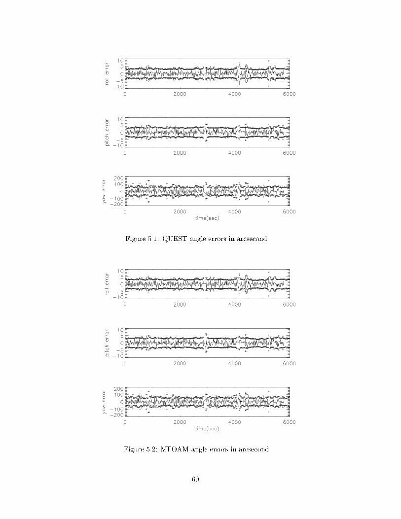
Figure 5.1: QUEST angle errors in arcsecond

Figure 5.2: MFOAM angle errors in arcsecond

60

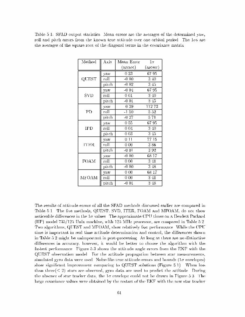
Table 5.1: SFAD output statistics. Mean errors are the averages of the determined yaw,roll and pitch errors from the known true attitude over one orbital period. The 1�s arethe averages of the square root of the diagonal terms in the covariance matrix.

Method Axis Mean Error 1�(arcsec) (arcsec)

yaw 0.23 67.95QUEST roll -0.00 3.40

pitch -0.02 3.45

yaw -0.04 67.95SVD roll 0.01 3.40

pitch -0.01 3.45

yaw -0.39 112.72PD roll -1.50 5.52

pitch -0.27 5.71

yaw 0.55 67.95IPD roll 0.04 3.40

pitch 0.03 3.45

yaw 0.11 77.15ITER roll 0.00 3.86

pitch -0.01 3.92

yaw -0.00 68.17FOAM roll 0.00 3.41

pitch -0.00 3.48

yaw 0.00 68.17MFOAM roll 0.00 3.41

pitch -0.01 3.48

The results of attitude errors of all the SFAD methods discussed earlier are compared inTable 5.1. The �ve methods, QUEST, SVD, ITER, FOAM and MFOAM, do not shownoticeable di�erences in the 1� values. The approximate CPU times on a Hewlett Packard(HP) model 735/125 Unix machine, with 125 MHz processor, are compared in Table 5.2.Two algorithms, QUEST and MFOAM, show relatively fast performance. While the CPUtime is important in real time attitude determination and control, the di�erences shownin Table 5.2 might be unimportant in post-processing. As long as there are no distinctivedi�erences in accuracy, however, it would be better to choose the algorithm with thefastest performance. Figure 5.3 shows the attitude angle errors from the EKF with theQUEST observation model. For the attitude propagation between star measurements,simulated gyro data were used. Noise-like true attitude errors and bounds (1� envelopes)show signi�cant improvement comparing to QUEST solutions (Figure 5.1). When lessthan three(� 2) stars are observed, gyro data are used to predict the attitude. Duringthe absence of star tracker data, the 1� envelope could not be drawn in Figure 5.3. Thelarge covariance values were obtained by the restart of the EKF with the new star tracker

61

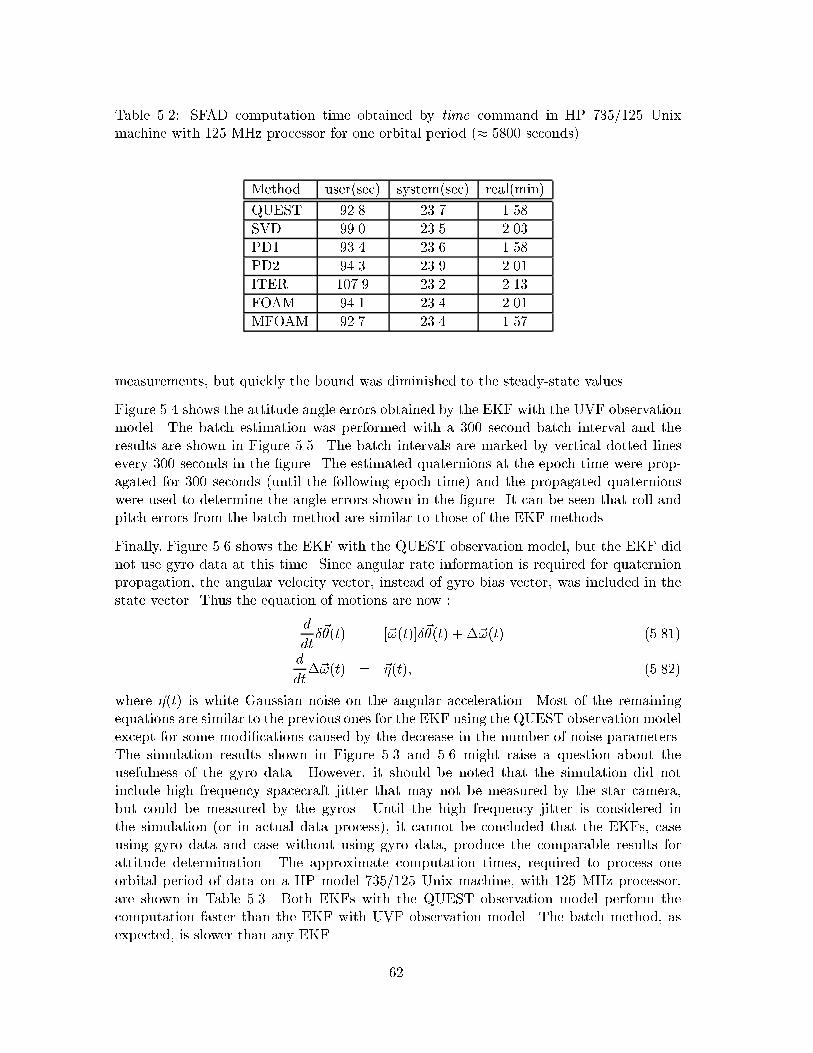
Table 5.2: SFAD computation time obtained by time command in HP 735/125 Unixmachine with 125 MHz processor for one orbital period (� 5800 seconds).

Method user(sec) system(sec) real(min)

QUEST 92.8 23.7 1.58

SVD 99.0 23.5 2.03

PD1 93.4 23.6 1.58

PD2 94.3 23.9 2.01

ITER 107.9 23.2 2.13

FOAM 94.1 23.4 2.01

MFOAM 92.7 23.4 1.57

measurements, but quickly the bound was diminished to the steady-state values.

Figure 5.4 shows the attitude angle errors obtained by the EKF with the UVF observationmodel. The batch estimation was performed with a 300 second batch interval and theresults are shown in Figure 5.5. The batch intervals are marked by vertical dotted linesevery 300 seconds in the �gure. The estimated quaternions at the epoch time were prop-agated for 300 seconds (until the following epoch time) and the propagated quaternionswere used to determine the angle errors shown in the �gure. It can be seen that roll andpitch errors from the batch method are similar to those of the EKF methods.

Finally, Figure 5.6 shows the EKF with the QUEST observation model, but the EKF didnot use gyro data at this time. Since angular rate information is required for quaternionpropagation, the angular velocity vector, instead of gyro bias vector, was included in thestate vector. Thus the equation of motions are now :

d

dt�~�(t) = [~!(t)]�~�(t) + �~!(t) (5.81)

d

dt�~!(t) = ~�(t); (5.82)

where ~�(t) is white Gaussian noise on the angular acceleration. Most of the remainingequations are similar to the previous ones for the EKF using the QUEST observation modelexcept for some modi�cations caused by the decrease in the number of noise parameters.The simulation results shown in Figure 5.3 and 5.6 might raise a question about theusefulness of the gyro data. However, it should be noted that the simulation did notinclude high frequency spacecraft jitter that may not be measured by the star camera,but could be measured by the gyros. Until the high frequency jitter is considered inthe simulation (or in actual data process), it cannot be concluded that the EKFs, caseusing gyro data and case without using gyro data, produce the comparable results forattitude determination. The approximate computation times, required to process oneorbital period of data on a HP model 735/125 Unix machine, with 125 MHz processor,are shown in Table 5.3. Both EKFs with the QUEST observation model perform thecomputation faster than the EKF with UVF observation model. The batch method, asexpected, is slower than any EKF.

62

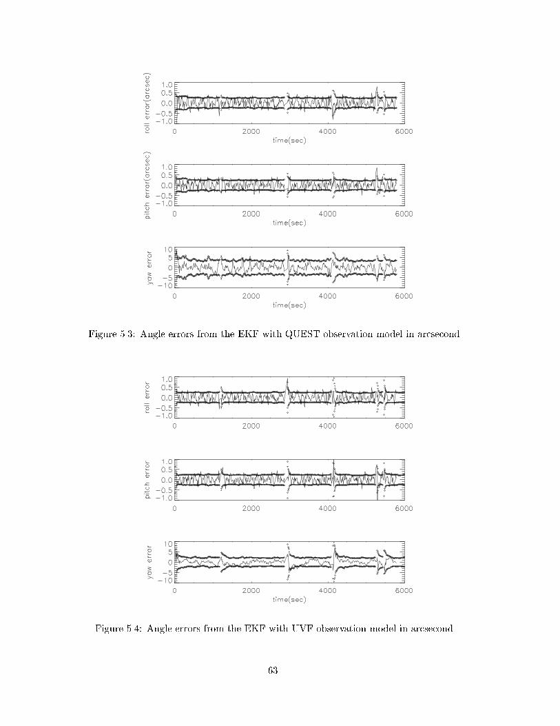
Figure 5.3: Angle errors from the EKF with QUEST observation model in arcsecond

Figure 5.4: Angle errors from the EKF with UVF observation model in arcsecond

63

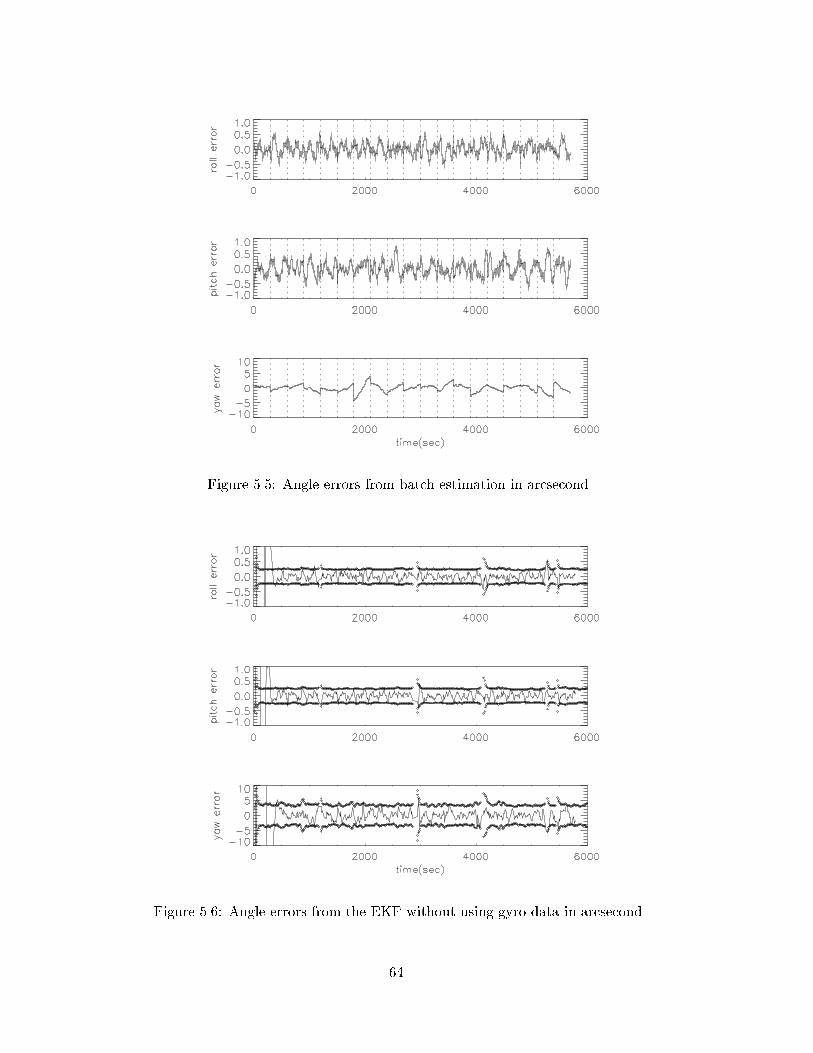
Figure 5.5: Angle errors from batch estimation in arcsecond

Figure 5.6: Angle errors from the EKF without using gyro data in arcsecond

64

Table 5.3: Computation time comparison

Method Obs. Model user(sec) system(sec) real(min)

EKF, QUEST, gyro 149.4 26.8 3.00

EKF, QUEST, non-gyro 143.9 24.7 2.51

EKF, UVF, gyro 341.5 10.1 6.00

BATCH, QUEST, gyro 451.2 92.0 9.08

Figure 5.7 shows the relation between true estimation errors and a 1� bound obtainedfrom the state error covariance matrix. The numbers on the line are associated with thetuning parameter, the process noise covariance matrix. As the number increases (12, 13� � � ), the magnitude of the process noise covariance matrix decreases. The EKF divergeswhen the process noise covariance matrix is too small.

Figure 5.7: True errors versus 1� values of EKF estimation (arcsecond)

Figure 5.8 shows the relation between true estimation errors and root mean squares (rms)of one orbital period EKF estimation. The trend of rms coincides with that of true errors.This particular case indicates the possibility of using rms values in the �lter tuning of theactual data where the true attitude is not known.

65

Figure 5.8: True errors versus rms values of EKF estimation (arcsecond)

66

Chapter 6

POINTING DETERMINATION

Figure 6.1 shows a conceptual sketch of the Stellar Reference System (SRS) which is beingdeveloped by Goddard Space Flight Center to measure the pointing angle of the GLASlaser beam to the required accuracy (less than 1.5 arcsecond, 1�), relative to the star�eld. To reduce the alignment exibility originating from multiple error sources, such asspacecraft jitter and temperature variation, all the components of the SRS will be at-tached to the GLAS optical bench. The SRS consists of a Laser Reference Camera (LRC)and the Attitude Determination System. The LRC contains optics, called Lateral TransferRetrore ectors (LTR), which are designed to extract and redirect onto the Laser ReferenceTelescope (LRT) both a portion of the outgoing laser pulse and a beam from a CollimatedReference Source (CRS). The CRS is rigidly attached to a side of the star tracker and pro-vides the alignment information of the star tracker. The LRT also observes a star (LRCstar) which is brighter than 7.5 visual magnitude. All of the images observed in the LRTare projected onto a 0:5� � 0:5� FOV Laser Reference Sensor (LRS). After locating theLRC star on the star �eld observed by the star tracker, other illuminated images in theLRS will subsequently be transformed to the star tracker star �eld in order to determinethe laser altimeter pointing direction in the SCF or the OBF. When the LRC star is notavailable, the CRS images projected to the LRS will be monitored to check the stability ofthe whole system on the optical bench while the rigid body assumption is being applied.While the GLAS laser is �red at a 40 Hz rate, the LRS sees the laser at 10 Hz. Theshot-to-shot direction of the laser beam is recorded by the Laser Pro�ling Array (LPA)with a frequency of 40 Hz. The centroids from 40 Hz laser images observed by the LPAmust be located in the LRS frame and consequently in the SCF. Ultimately, the propercoordinate transformations would give us the 40 Hz laser beam pointing direction in boththe TRF and the CRF. The details of the SRS instruments, such as mechanical require-ments, design concepts, construction materials and statistical quantities, are provided inthe GLAS Critical Design Review [47].

6.1 POINTING DETERMINATION ALGORITHM

Once a star observed in either the LRS or by the star tracker is identi�ed, the star appearsas a static point source in the CRF (see Star Catalog in Figure 6.2). The identi�ed

67

StarTracker4-10Hz CRS

CollimatedReferenceSource

�

Semi-transparentLTR

�

CRS

�

Allign.LTR's�

?

Laser ReferenceTelescope, F/6(Newtonian)

� OLaser Ref.Sensor10 Hz

LRS(CCD Array)

BPF/lensLPA

40Hz

80�80CCD

GLAS Laser40 pps

NADIR

Semi-transparentLTR's

��

�

?

Star Field

6

ZENITHLRC

Laser Reference CameraADS

Attitude Det. System

GyroHRG

Laser Pro�lling ArrayImage Frame

GLASLaser

1.3�1.3 mrad FOV(0:08� � 0:08�)80�80 array

Laser Ref. CameraImage Frame

8.5�8.5 mrad (0:5� � 0:5�) FOV512� 512 array

CRSST

GLASLaser

Star

Star TrackerImage Frame

8� � 8� FOV512� 512 array

LRC FOV

Star

-�

Figure 6.1: Stellar Reference System

68

b

r

r

r

r

r

r

r

+

?

LRS Star Identi�cation

6

Star Identi�cation

(Attitude Determination)

LRS

Star Tracker Star Catalog

�Ma

q

-M�1

Figure 6.2: Pointing determination using the Stellar Reference System

tracker stars will allow us to determine the attitude, A(t), at time t by applying attitudedetermination algorithms. The attitude matrix transforms the star coordinates in theCRF into those in the instrument OBF. If the alignment matrix, S(t), which transformsthe star coordinates in the OBF into those in the SCF, is temporarily presumed constant,the combined matrix, M(t) :

M(t) = S(t)A(t) (6.1)

describes the coordinate transformation from the CRF to the SCF. Once the matrix,M(t),is determined at every measurement time t, the LRC star identi�ed in the CRF can betransformed to a dotted line at the star tracker FOV (see Star Tracker in Figure 6.2). Thetracks of the LRC star both in the star tracker FOV and in the LRS FOV are input datato the least squares method which will be introduced in the following subsection. If thestar in the LRC is brighter than magnitude 6, it will also be seen in the star tracker sothat the projected LRC star positions on the star tracker FOV can be veri�ed/calibratedwith the observed star by the star tracker itself.

6.1.1 Estimation of the LRS frame in terms of the SCF

Figure 6.3 describes the overlap of the LRS FOV on the star tracker FOV, but the LRSFOV is oversized to well visualize the relation between the two FOVs. Ideally, the twoframes share the common origin. In the real situation, there might be an o�set between thetwo origins. This o�set is represented as the coordinate of the LRS origin, (xoffset; yoffset),in terms of the SCF. In addition, the LRS FOV might rotate by angle � against the SCF.Finally, the magnitude ratio of two FOVs, F , might change if focal lengths vary. Once we

69

Star Tracker

+ F l

LRS

����

�

AAAAA

AAAAA

AAAAAAAAAA

����

�

+

l

�

xoffset

yoffset

star

b

b

Nominal Values :

xoffset = yoffset = 0:0

� = 0; F = 16

Figure 6.3: Estimation parameters for coordinate transformation between LRS frame andSCF

know these o�set parameters, (xoffset; yoffset; �; F ), any point in the LRS FOV can beprojected into the star tracker FOV using the following equation :�

xstarLRSystarLRS

�= F

�cos � sin �

� sin � cos �

� �xstarST � xoffsetystarST � yoffset

�: (6.2)

where (xstarLRS ; ystarLRS ) is the coordinate of the LRC star in the LRS frame and(xstarST ; ystarST ) is the coordinate of the same star in the SCF. Considering the velocityof the GLAS/ICESAT and the size of the LRS FOV, we will have approximately 80 points(i.e. 8 seconds) of the consecutive LRC star measurements in both FOVs. With thesedata, the o�set parameters can be estimated by applying the least squares method [45] tothe Equation 6.2. Finally, Equation 6.2 is used to locate the laser point in the star trackerFOV by inserting the estimated parameters, xoffset; yoffset; � and F :�

xlaserLRSylaserLRS

�= F

�cos � sin �

� sin � cos �

� �xlaserST � xoffsetylaserST � yoffset

�; (6.3)

where (xlaserLRS ; ylaserLRS) are the coordinates of the LRS laser in the LRS frame and(xlaserST ; ylaserST ) are the coordinates of the same laser point located in the SCF. Equa-tion 6.3 is also used for the projection of the CRS point. After the laser points observedin the LRS FOV are located in the SCF, direction cosines (i.e. unit vector for the laserpointing direction) can be restored by considering the focal length of the star tracker.The construction of the laser pointing vector will be made once the laser travel time (i.e.range) is determined. The inverse of the matrix M(t), M(t)�1, should be applied to

70

Figure 6.4: Pointing determination simulation result (10Hz)

transform the laser coordinates from the SCF to the CRF. As discussed at the end ofSection 1.1, the laser spot position vector will be obtained by appropriately combining thelaser pointing vector with the laser pulse travel time and the POD position vector. Thespot location will be produced in the Earth-�xed axes, speci�cally ITRF by the propercoordinate transformation [32].

A simulation result for GLAS laser pointing determination is shown in Figure 6.4. TheLRC star measurement data were created from a star catalog which contains 32511 starsranging down to magnitude 7.5. The LRC star measurement noise was in the range of 0.2to 0.4 arcsecond depending on the star brightness [47]. In addition to the random noise inthe overall SRS, the true shot-to-shot variation of the laser beam direction was given as0.3 arcsecond (1�). The pointing errors in the �gure are the absolute di�erences betweenthe true and the estimated pointing directions. For the most part, the pointing errors werebelow 1.5 arcseconds, satisfying the accuracy requirement.

6.1.2 Absence of the LRC Star

As shown in Figure 6.4, a half degree LRS FOV will occasionally observe stars. The timeduration before a new star comes in to the LRS appears to be within a few minutes inthe �gure. To determine the maximum or average time between LRC star observations,simulations covering the whole sky might be necessary. The probability computation of thestar tracker's star observations, from both theory and simulation, indicated that the starsin our universe do not deviate considerably from the random distribution (see Table 3.4).Using the Poisson distribution[50], the computation shows that, during an orbital periodof the GLAS, a star will be observed in the LRS more than 100 occasions, meaning at leasta star per minute. Therefore, the LRS would almost always observe a new star withinseveral minutes after the dropout of an old one, especially in the polar regions where no

71

Figure 6.5: Pointing determination simulation result (10Hz, �lled)

solar or lunar blocking would occur. Expecting that the line of sight stability for theGLAS optical bench would be less than 0.1 arcsecond(1�) during one orbital period [27][33], we conclude that the o�set parameters obtained during a LRC star observation canbe used after the star leaves the LRS FOV. When a new star comes into the LRS, theparameters will be updated and used until another new star is observed. If a noticablechange of instrument alignment between star tracker and LRS occurs, it would be detectedby monitoring the CRS points since the LRS also observes the CRS images projected fromthe star tracker CRS. Figure 6.5 shows the simulation results after �lling up intervalsbetween LRS observations using constant o�set parameters before a new star.

6.1.3 LPA measurement projection into LRS frame

While the LRS sees star, laser and CRS points at a 10Hz rate, the LPA observes the laserbeam at a 40Hz rate. The position of the laser in the LPA needs to be located in the LRSin order to determine the 40Hz laser beam pointing direction in the CRF. Although theLPA consists of an array of 80 by 80 pixels, only 20 by 20 array containing the laser pointnear its center will be read. An example of the laser pro�le is shown in Figure 6.6. Amethod to �nd the centroid (xi;LPA; yi;LPA) of the laser image is :

xi;LPA =

P201 n

P201 m Im;nP20

1

P201 n m Im;n

yi;LPA =

P201 m

P201 n Im;nP20

1

P201 n m Im;n

(6.4)

where Im;n is the laser intensity of m row and n column.

Pre-launch calibration will provide the formula to project the LPA laser point to the LRSframe. However, the relative position of the LPA frame with respect to the LRS frame

72

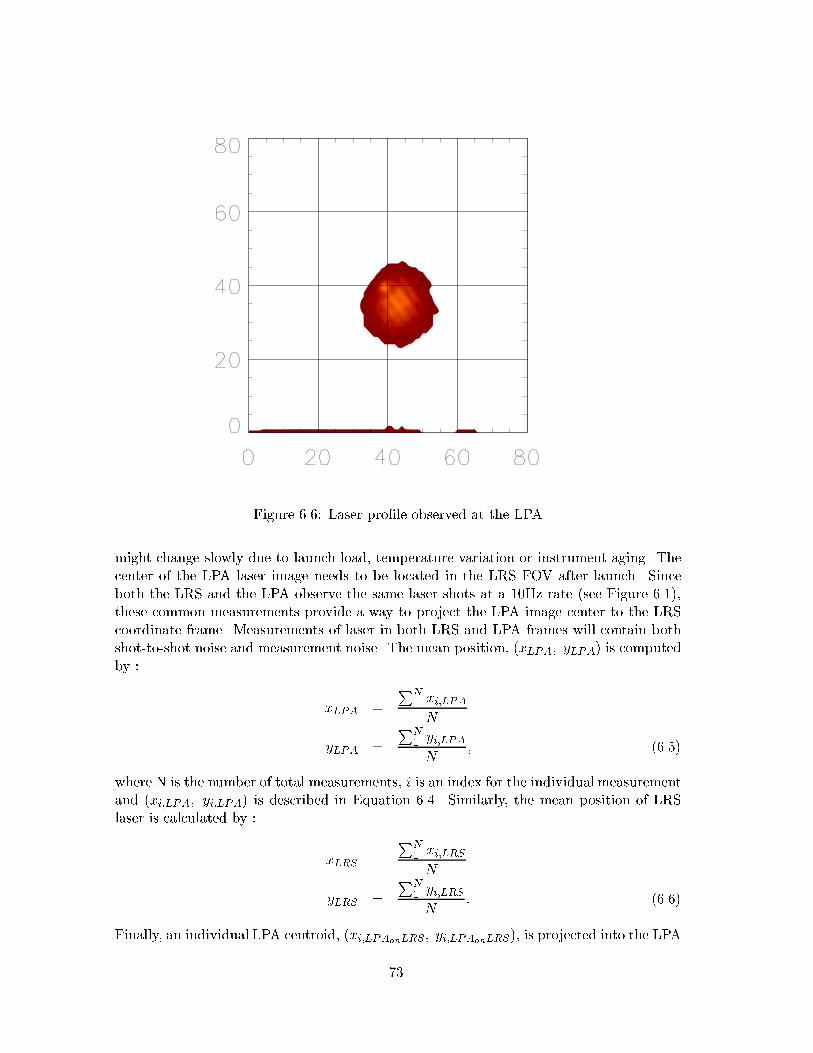
Figure 6.6: Laser pro�le observed at the LPA

might change slowly due to launch load, temperature variation or instrument aging. Thecenter of the LPA laser image needs to be located in the LRS FOV after launch. Sinceboth the LRS and the LPA observe the same laser shots at a 10Hz rate (see Figure 6.1),these common measurements provide a way to project the LPA image center to the LRScoordinate frame. Measurements of laser in both LRS and LPA frames will contain bothshot-to-shot noise and measurement noise. The mean position, (xLPA; yLPA) is computedby :

xLPA =

PN1 xi;LPAN

yLPA =

PN1 yi;LPAN

; (6.5)

where N is the number of total measurements, i is an index for the individual measurementand (xi;LPA; yi;LPA) is described in Equation 6.4. Similarly, the mean position of LRSlaser is calculated by :

xLRS =

PN1 xi;LRSN

yLRS =

PN1 yi;LRSN

: (6.6)

Finally, an individual LPA centroid, (xi;LPAonLRS ; yi;LPAonLRS), is projected into the LPA

73

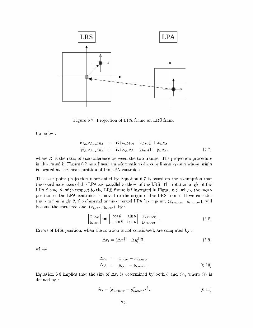
LRS LPA

Figure 6.7: Projection of LPA frame on LRS frame

frame by :

xi;LPAonLRS = K(xi;LPA � xLPA) + xLRS

yi;LPAonLRS = K(yi;LPA � yLPA) + yLRS ; (6.7)

where K is the ratio of size di�erence between the two frames. The projection procedureis illustrated in Figure 6.7 as a linear transformation of a coordinate system whose originis located at the mean position of the LPA centroids.

The laser point projection represented by Equation 6.7 is based on the assumption thatthe coordinate axes of the LPA are parallel to those of the LRS. The rotation angle of theLPA frame, �, with respect to the LRS frame is illustrated in Figure 6.8 where the meanposition of the LPA centroids is moved to the origin of the LRS frame. If we considerthe rotation angle �, the observed or uncorrected LPA laser point, (xi;uncor; yi;uncor), willbecome the corrected one, (xi;cor; yi;cor), by :�

xi;coryi;cor

�=

�cos � sin �� sin � cos �

� �xi;uncoryi;uncor

�: (6.8)

Errors of LPA position, when the rotation is not considered, are computed by :

�ri = (�x2i +�y2i )1

2 ; (6.9)

where

�xi = xi;cor � xi;uncor

�yi = yi;cor � yi;uncor: (6.10)

Equation 6.8 implies that the size of �ri is determined by both � and �ri, where �ri isde�ned by :

�ri = (x2i;uncor + y2i;uncor)1

2 : (6.11)

74

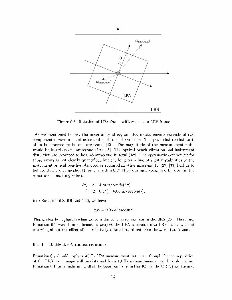
(xLRS, yLRS)

(xLPA, yLPA)

LRS

LPA

Figure 6.8: Rotation of LPA frame with respect to LRS frame

As we mentioned before, the uncertainty of �ri on LPA measurements consists of twocomponents: measurement noise and shot-to-shot variation. The peak shot-to-shot vari-ation is expected to be one arcsecond [40]. The magnitude of the measurement noisewould be less than one arcsecond (1�) [25]. The optical bench vibration and instrumentdistortion are expected to be 0.45 arcsecond in total (1�). The systematic component forthose errors is not clearly quanti�ed, but the long term line of sight instabilities of theinstrument optical benches observed or required in other missions [13] [27] [33] lead us tobelieve that the value should remain within 0:5� (3 �) during 5 years in orbit even in theworst case. Inserting values

�ri < 4 arcseconds(3�)

� � 0:5�(= 1800 arcseconds);

into Equation 6.8, 6.9 and 6.10, we have

�ri = 0:06 arcsecond:

This is clearly negligible when we consider other error sources in the SRS [25]. Therefore,Equation 6.7 would be su�cient to project the LPA centroids into LRS frame withoutworrying about the e�ect of the relatively rotated coordinate axes between two frames.

6.1.4 40 Hz LPA measurements

Equation 6.7 should apply to 40 Hz LPA measurement data even though the mean positionof the LRS laser image will be obtained from 10 Hz measurement data. In order to useEquation 6.1 for transforming all of the laser points from the SCF to the CRF, the attitude,

75

A(t), needs to be known at a 40 Hz rate. Since the attitude, A(t), is determined fromstar tracker and gyro data whose measurement rates are only 10 Hz, a linear interpolationis required to get the instrument attitude at 40 Hz. This interpolation can be justi�edonly if the LPA frame is relatively �xed with respect to the LRS frame during the intervalin which the interpolation is applied (i.e. 1 second). If the instrument or optical benchhas signi�cant high frequency jitter, the interpolated attitude might produce unacceptablepointing error, then it might be necessary to use gyros capable of 20 Hz or 40 Hz ratemeasurements.

Figure 6.9 illustrates the overall measurement relations between star tracker, LRS andLPA. The �nal products of the PAD are laser pointing unit vectors in both ICRF andITRF.

6.1.5 Collimated Reference Source (CRS)

The CRS, which will be mounted kinematically to the reference surface on the star tracker,will maintain true pointing direction and collimation of its own laser pulse. The stabilityrequirement is 0.2 arcseconds (1�) over a �0:5�C gradient [47]. From the error sourcesin the relay of the CRS beam including LRT distortion and LRC centroid error, themeasurement error in the LRC is expected to be similar to that of the LRC star. Themonitoring of the CRS beam image over time will allow us to monitor the SRS structurestability and to verify the image quality in the LRC. Furthermore, during the loss of startracker data due to, for example, solar and lunar eclipsing - the maximum duration is about20 minutes (see Section 3.3) - the o�set parameters in Equation 6.2 may be presumed asconstants if the CRS image remains in the stable position without any systematic change.The angular diameters of the Sun and the Moon are both approximately 0:5�, which isthe size of the LRC FOV. As long as the LRC is not under the direct illumination of theSun or the Moon, the LRC is expected to provide centroids of both CRS and laser imagesat the 10 Hz rate. By applying the algorithm depicted in the previous sections, the 40 Hzlaser pointing determination will be available with the LPA laser images.

6.2 Spacecraft Velocity In uence on Laser Pointing

In Section 3.3.3, a simpli�ed algorithm, to correct the stellar aberration, was shown. ThePAD of the spacecraft is determined within the CRF and must be corrected for this e�ect,stellar aberration being the result of the spacecraft (and the star tracker) motion withrespect to the relatively �xed stars. In like manner, the motion of the spacecraft withrespect to a point on the surface of the Earth will cause a similar e�ect that can betentatively called pointing aberration. Figure 6.10 illustrates both stellar and pointingaberrations. Since the aberration is a function of relative velocity, and not the distance,between the observer and the source, the same algorithm can be applied. For pointingaberration, the applicable velocity is the relative velocity of the Earth with respect to thespacecraft. The magnitude of the pointing aberration can be calculated by Equation 3.14

76

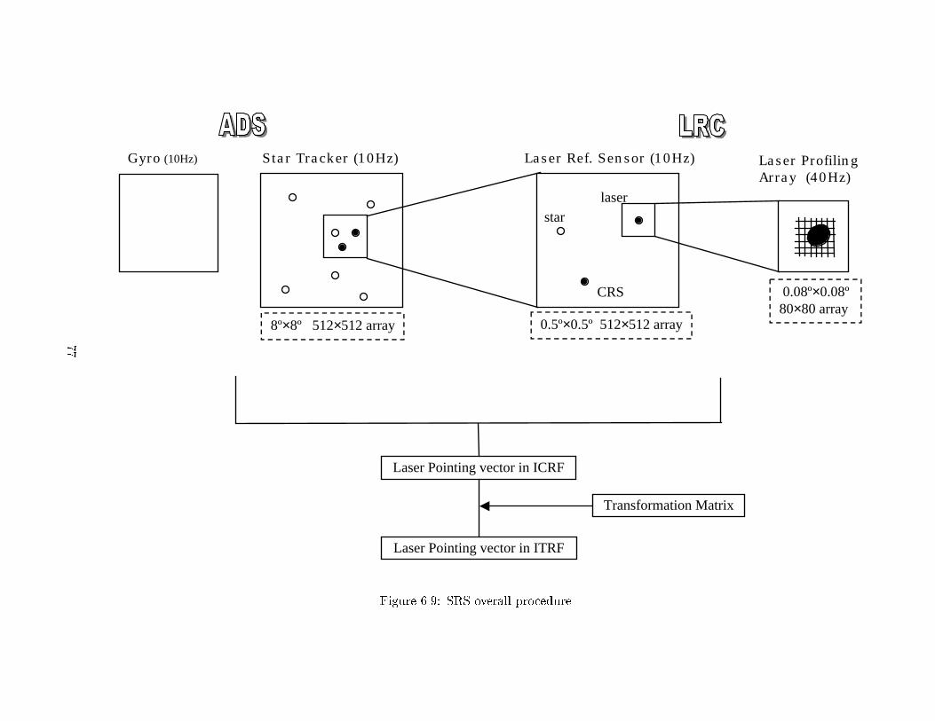
Gyro (10Hz) Star Tracker (10Hz) Laser Ref. Sensor (10Hz) Laser ProfilingArray (40Hz)

Laser Pointing vector in ICRF

Laser Pointing vector in ITRF

Transformation Matrix

8º×8º 512×512 array 0.5º×0.5º 512×512 array

0.08º×0.08º80×80 array

laser

star

CRS

Figure 6.9: SRS overall procedure

77

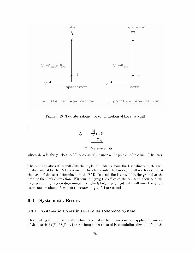
spacecraftV

star spacecraft

V

^

Earth

V = V earth+ Vs/c V = -Vs/c

a. stellar aberration b. pointing aberration

-ps

Figure 6.10: Two aberrations due to the motion of the spacecraft

:

�p =j~vjcsin �

=j � ~vs=cj

c�= 5:2 arcseconds

where the � is always close to 90� because of the near-nadir pointing direction of the laser.

The pointing aberration will shift the angle of incidence from the laser direction that willbe determined by the PAD processing. In other words, the laser spot will not be located atthe path of the laser determined by the PAD. Instead, the laser will hit the ground at thepath of the shifted direction. Without applying the e�ect of the pointing aberration thelaser pointing direction determined from the GLAS instrument data will miss the actuallaser spot by about 15 meters corresponding to 5.2 arcseconds.

6.3 Systematic Errors

6.3.1 Systematic Errors in the Stellar Reference System

The pointing determination algorithm described in the previous section applied the inverseof the matrix M(t), M(t)�1, to transform the estimated laser pointing direction from the

78

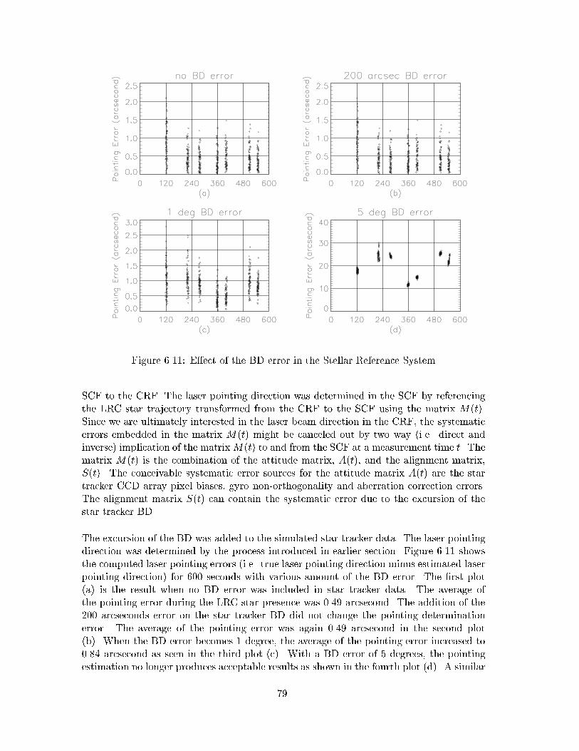
Figure 6.11: E�ect of the BD error in the Stellar Reference System

SCF to the CRF. The laser pointing direction was determined in the SCF by referencingthe LRC star trajectory transformed from the CRF to the SCF using the matrix M(t).Since we are ultimately interested in the laser beam direction in the CRF, the systematicerrors embedded in the matrix M(t) might be canceled out by two way (i.e. direct andinverse) implication of the matrixM(t) to and from the SCF at a measurement time t. Thematrix M(t) is the combination of the attitude matrix, A(t), and the alignment matrix,S(t). The conceivable systematic error sources for the attitude matrix A(t) are the startracker CCD array pixel biases, gyro non-orthogonality and aberration correction errors.The alignment matrix S(t) can contain the systematic error due to the excursion of thestar tracker BD.

The excursion of the BD was added to the simulated star tracker data. The laser pointingdirection was determined by the process introduced in earlier section. Figure 6.11 showsthe computed laser pointing errors (i.e. true laser pointing direction minus estimated laserpointing direction) for 600 seconds with various amount of the BD error. The �rst plot(a) is the result when no BD error was included in star tracker data. The average ofthe pointing error during the LRC star presence was 0.49 arcsecond. The addition of the200 arcseconds error on the star tracker BD did not change the pointing determinationerror. The average of the pointing error was again 0.49 arcsecond in the second plot(b). When the BD error becomes 1 degree, the average of the pointing error increased to0.84 arcsecond as seen in the third plot (c). With a BD error of 5 degrees, the pointingestimation no longer produces acceptable results as shown in the fourth plot (d). A similar

79

simulation can be applied for the e�ect of the systematic errors included in the attitudematrix A(t). However, di�erent approaches for the attitude systematic errors are discussedin the following section.

6.3.2 Systematic Errors in Attitude Determination

A Ball CT-601 star tracker was used for the high accuracy attitude determination ofthe Midcourse Space Experiment (MSX) mission [12]. The highest accuracy that theMSX had to achieve for the instrument pointing stability was 2 arcseconds (1�). Whilethe pre-launch simulation showed the ful�llment of the attitude determination/pointingrequirement, the MSX could not determine the attitude to the required accuracy from theactual star tracker and gyro data. In the attitude determination simulation before launch,some fundamental assumptions were made. Eventually, the assumptions turned out tobe inadequate for the actual data processing. One of these assumptions concerned thecharacteristics of the star tracker measurement errors. While these errors were presumedto be adequately modeled as white noise in the simulation, the individual pixel of thestar tracker CCD array included its own bias, eventually, resulting in the error of the starimage centroid. Since the e�ect of the systematic error can not be removed by the usualstatistical estimation procedures, the attitude determined by the white noise assumptioncould not satisfy the accuracy requirement.

While the MSX is completely versatile, with science scenarios varying from inertial stares towhole sky scans to tracking satellites, ballistic missiles and their surrogates, and coveringabout anything in between, the GLAS/ICESAT will maintain one attitude scenario :altimeter laser pointing toward the near-nadir direction in near-circular and near-polarorbit. A star would come in and move across the 8� � 8� FOV with a relatively constantrate for about 4 minutes until it exits. By considering 512 by 512 pixels in the CCDarray, a star will stay on a pixel about 0.25 seconds. Unlike the case of the inertial staringattitude where one pixel sees a star for long duration, the pixel's local bias will a�ectthe star measurement in two or three snaps, and then the star moves into the next pixelthat would be characterized by its own size and direction for bias. Moreover, the attitudedetermination algorithms will utilize multiple stars which will be located at all di�erentpixels in the tracker CCD array at a measurement time. In this situation, the change ofpixel biases of �ve or six star observations should be considered as random and the residuale�ect of the systematic error sources would be negligible.

By using the bias correction tables within the post facto attitude determination software,the Roentgen Satellite (ROSAT) mission corrected the star tracker cameras' measurementsin pointing mode [30]. For the GLAS, it is expected that the manufacturer will providethe built-in bias calibration function of the star tracker [40] to remove both the individualpixel biases and the large distortion of the CCD array before the data are actually taken.This self-calibration ability of the star tracker will, at least, reduce the size of the biaserrors signi�cantly, if not remove them completely.

The SRS ability to cancel out the measurement systematic error was also discussed in theprevious section. The laser pointing determination algorithm using the specially designedSRS will avoid the systematic errors embedded in the alignment matrix S(t), as well as

80

in the attitude matrix A(t). When we consider only instrument pointing determination,the SRS should be able to remove the e�ects of many systematic error sources even at theinertially staring attitude mode of the spacecraft.

Besides the white noise model for the star tracker measurements, another inadequateassumption for the MSX attitude determination system was the obtainability of the un-interrupted star tracker attitude data at its nominal update rate of � 9 Hz. Extensiveanalytic studies indicated fairly strongly that glint from the Sun is a signi�cant problem,possibly because of unanticipated re ections o� the SPIRIT III (one of the MSX's instru-ment) shield [12]. The unexpected glint would require the tracker integration time to belonger than anticipated, which will result in the large image smearing and interrupted datarate. The Kalman �lters and the batch algorithm introduced in Chapter 2 are capableof estimating the gyro biases as well as the spacecraft attitude quaternions. The highfrequency attitude update due to 10 Hz star tracker measurement rate will make the gyrobiases include not only true bias but also other e�ects such as gyro non-orthogonality,gravity or magnetic e�ects [46]. Since the star tracker and gyro unit are located on the op-tical bench which is designed to hold the rigidity between instruments, the self-calibratingcapability of gyro systematic errors by estimating gyro biases will be kept as long as thestar tracker provides high frequency observations. The failure to achieve the star trackermeasurements at the anticipated rate probably made the MSX attitude determinationsu�er from the MSX gyros systematic errors other than true biases. The GLAS requiresthe precise attitude/pointing determination in the high latitude regions such as Greenlandand Antarctica (j�j > 60�). Since the Sun and the Moon, the possible cause of the glint,are located near the ecliptic plane (j�j � 23:5�), the e�ect of the Sun and the Moon lighton the star tracker measurement should be minimal and uninterrupted tracker data rateis expected. Consequently, the Kalman �lter that estimates both the attitude quaternionsand the gyro bias simultaneously would provide the auto-calibration feature for the gyro'ssystematic errors, if the HRG of the GLAS su�ers from problems similar to the MSX gyro.

81

Chapter 7

IMPLEMENTATION

CONSIDERATIONS

7.1 Standards

To facilitate generation of the laser pointing direction, the attitude should be expressedusing reference frames common to those used in description of the orbit position. Asdiscussed by Rim and Schutz [28], the POD process will provide the position of the space-craft/instrument center of mass in the ICRF which is the speci�c implementation of theCRF. The determination of the transformation matrix between the spacecraft-�xed axesand the CRF depends, in part, on the adopted star catalog used with the analysis of starcamera data. In mid 1997, the Hipparcos star catalog was released containing more than100,000 sources with position precision better than one mas (see Table 3.5). Althoughadditional analysis will be required, it is expected that the Hipparcos catalog will be thefoundation of the GLAS PAD. Additional stars were available with the Hipparcos release,known as the Tycho catalog, but with precision at the 30 mas level. Nevertheless, the Ty-cho contribution contains about one million stars. The Hipparcos source coordinates willbe de�ned for an epoch corresponding to J2000 and the reference system will be realizedthrough the ICRF. The proper motions in the catalog are better than 1 mas/yr. The Hip-parcos catalog will link the optical sources (used by Hipparcos) to the radio sources (usedby the IERS) at a level better than 1 mas [20]. Further discussion is given by McCarthy[24].

Conceptually, the determination of the laser spot location will be determined in the ICRFusing the spacecraft center of mass ephemeris from the POD and the transformation ma-trix from the PAD to determine the measured height vector. This height vector will betransformed into the ITRF using the IERS measured UT1, as well as precession and nu-tation parameters. The same transformation between the ICRF and the ITRF is requiredin the POD process. The transformation into the ITRF from the ICRF is well establishedat the milliarcsecond level.

82

7.2 Ancillary Inputs

Ancillary inputs include the Hipparcos and Tycho star catalogs and a luni-solar-planetaryephemerides, such as DE-200 or later [42]. The latter complements the star catalog byenabling identi�cation of solar system bodies in camera images. For the generation ofthe transformation between the spacecraft-�xed axes and the ICRF, the velocity aberra-tion corrections of the observed stars are needed (see Section 3.3.3 and Table 7.1). Theephemeris of the GLAS satellite determined in the POD processing will be known withaccuracy better than the real time ight operations ephemeris. In addition, to expeditethe PAD process, access to the real time attitude determination from the ight operationssegment is required. This information will reduce the search time to identify stars in thestar camera images by providing a priori attitude information of modest accuracy.

The POD process requires real time attitude information as well as a modest accuracy apriori ephemeris. The present algorithm development will pursue independent POD andPAD processes to simplify software validation, even though these processes (including thelaser pointing process) share common aspects. The common parameters will be madeavailable through shared �les.

7.3 Accuracy and Validation

An estimate of the attitude determination accuracy is shown in Table 7.1 [47]. Whilethe star catalog is expected to introduce no signi�cant errors into the estimation process,the star camera will be the dominant source of error. The RSS of roll and pitch, whichwill a�ect the laser pointing direction, is 0.85 arcsecond. The overall RSS of all the errorsources for the laser pointing determination is expected to be 1.20 arcsecond (1�) (seeTable 1.1). The simulation in this document did not include unmeasured errors, stemmingfrom the unsensed bench vibration and the unsensed angular distortions. Even thoughthe pointing errors shown in the plots in Chapter 6 will increase slightly when theseunmeasured errors are taken into account, the resultant 1� value should be smaller than1.20 arcsecond considering the magnitude of the unmeasured errors and our simulationresults.

Detailed discussion for the attitude validation is contained in the Calibration/ValidationPlan [48]. In summary, a �rst order validation of attitude will be conducted by comparisons

Table 7.1: Overall attitude determination accuracy goal

roll(arcsec) pitch(arcsec)

1.Attitude Determination 0.47 0.47

2.Velocity Aberration 0.03 0.03

3.Star Position Accuracy 0.03 0.03

4.Ephemeris 0.01 0.01

RSS(2,3,4) + 1 0.52 0.52

83

with the real time determination. This approach, however, is limited because the real timerequirements are about 10-20 arcseconds (1�), compared to 1 arcsecond (1�) required forscience analysis. As described in this plan, validation of the attitude at the 1 arcsecondlevel is inherently linked to laser pointing. Experiments to validate the laser pointing willsimultaneously assess the PAD.

7.4 Computational: CPU, Memory and Disk Storage

The Hipparcos catalog contains approximately 120000 stars. This catalog contains infor-mation about star characteristics, as well as the star coordinates to a resolution of 1 mas.The storage requirements are approximately 100 MB for the star catalog. The memoryrequirements for the estimation process are less than 64 MB. The requirements for theproduct of the PAD, the 3 � 3 transformation matrix between spacecraft-�xed axes andthe ICRF, will require about 300 MB/day. Alternatively, about 150 MB/day would berequired if 4 quaternion elements were used at each time instead of 9 matrix elements.Preliminary tests show that an HP735-level machine can support the required attitude de-termination; however, further tests will be conducted to provide a more de�nitive estimatefor CPU, memory and disk storage.

The approximate CPU times for one orbital period of data processed with the EKF algo-rithms on a HP model 735/125 Unix machine were given in Table 5.2. From the table, theprocessing time for one day attitude of data is estimated to be approximately 45 minutesfor the EKF using the QUEST observation model and 90 minutes for the one using theUVF model. The batch algorithm is expected to require about 135 minutes for the sameamount of data. The overall PAD process will require additional CPU time for the SRSdata processing discussed in Chapter 6 and the data preprocessing.

7.5 Sensor Failures

Although the PAD study has been done with a star tracker in the instrument opticalbench, there will exist two additional CCD star trackers (Ball CT-602) mounted on thespacecraft structure. The primary purpose of the spacecraft star trackers is to providedata for the real time attitude determination. The spacecraft star tracker data will beavailable on the ground and the additional star measurement data can be used for PADin post-processing. Since the BDs of the CT-602 star trackers will not be parallel to thatof the instrument star tracker, the contribution of this star tracker to the determinationof the laser pointing direction is limited by the amount of the angle between star trackers'BDs. However, in case the instrument star tracker malfunctions, the Ball CT-602 startrackers' data must be used to produce the best laser pointing information.

This idea can be extended when the optical bench star tracker loses data temporarily dueto solar and lunar eclipsing with no permanent failure. Instead of totally depending on theCRS image stability as discussed in Section 6.1.5, it might be possible to use the attitudesobtained by the CT-602 star trackers whose BDs are 45� away from the optical bench

84

star tracker. The calibrated data of the CT-602 trackers in terms of the instrument startracker will provide 10 Hz attitude determination for the PAD with degraded accuracy.

Meanwhile, the situation is not the same for gyro failure since there is no alternative systemin the spacecraft. There are two possible ways to generate angular rates without the actualrate measurement even though the accuracy level is in doubt. The �rst choice is to use theEuler equation (Equation 2.18) to compute the spacecraft angular rates. For this case, thenumerical or analytical expression for external torques must be modeled as a function oftime as well as a function of the position and attitude of the spacecraft. The other choiceis already mentioned in Section 5.4 when the EKF simulation results were discussed. TheEKF without using gyro data showed equal or better accuracy in attitude determination.However, it was indicated that the real spacecraft motion may contain high frequencynoise which can be detected only by gyros. Even though the replaced system/methodto the original PAD system will not determine the attitude to the required accuracylevel, preparation of alternatives to produce the most accurate attitude determination asa backup plan is prudent.

85

Bibliography

[1] European Space Agency. The Hipparcos and Tycho Catalogues. ESA PublicationsDivision, 1997.

[2] Ball Aerospace Engineering. CT-601 Solid-State Star Tracker.

[3] I.Y. Bar-Itzhack. Polar decomposition for attitude determination from vector obser-vation. AIAA, (92-4545), 1992.

[4] C. Buil. CCD Astronomy : Construction and Use of an Astronomical CCD Camera.Willmann-Bell, Richmond, Va., 1st English edition, 1991.

[5] L.W. Cassidy. Miniature star tracker for precise attitude reference in space. TechnicalReport PA 1868, Hughes Danbury Optical Systems, Inc., 1995.

[6] V. Chobotov. Spacecraft Attitude Dynamics and Control. Krieger Publishing Co.,Malabar, 1991.

[7] Raytheon Systems Company. GLAS Star Tracker Test Results. Systems EngineeringMemorandum, March 2000.

[8] R.L. Farrenkopf. Analytic steady-state accuracy solutions for two common spacecraftattitude estimators. Journal of Guidance and Control, 1(4), Jul{Aug 1978.

[9] D.R. Fink, K.B. Chapman, W.S. Davis, J.A. Hashmall, S.E. Shulman, S.C. Under-wood, J.M. Zsoldos, and R.R. Harman. Experience gained from launch and early orbitsupport of the Rossi X-ray Timing Explorer(RXTE). In Flight Mechanics/EstimationTheory Symposium, Publication 3333. National Aeronautics and Space Administra-tion Conference, May 1996.

[10] H.L. Fisher, M.D. Shuster, and T.E. Strikwerda. Attitude determination for the startracker mission. AAS, (89-365), 1989.

[11] D.T. Greenwood. Principles of Dynamics. Prentice-Hall, Inc., New Jersey, 1988.

[12] D.R. Haley, T.E. Strikwerda, H.L. Fisher, and G.A. Heyler. Attainable pointingaccuracy with star trackers. AAS, (98-072), 1998.

[13] K.A. Havey, G.L. Compagna, and N. Lynch. Precision Thermal Control Trades forTelescope Systems. SPIE, 3356, 1998.

86

[14] S.B. Howell, editor. Astronomical CCD Observing and Reduction Techniques, vol-ume 23 of Astronomical Society of the Paci�c conference series, San Francisco, Cali-fornia, 1992. Astronomical Society of the Paci�c.

[15] J.L. Junkins and J.D. Turner. Optimal Spacecraft Rotational Maneuvers. ElsevierPublishing Company, New York, 1986.

[16] E.J. Le�erts, F.L. Markley, and M.D. Shuster. Kalman �ltering for spacecraft attitudeestimation. Journal of Guidance, Control, and Dynamics, 5(5), 1982.

[17] I.T. Lewis, A.G. Ledebuhr, T.S. Axelrod, J.F. Kordas, and R.F. Hills. WFOV startracker camera. Sensors and Sensor Systems for Guidance and Navigation, SPIE,1478, 1991.

[18] C.C. Liebe. Star trackers for attitude determination. IEEE Aerospace and ElectronicSystems Magazine, Jun 1995.

[19] S. Lim and B.E. Schutz. Repeat ground track analysis for the geoscience laser altime-ter system. AAS, (96-205), 1996.

[20] L. Lindegren and J. Kovalevsky. Linking the Hipparcos catalogue to the extragalacticreference frame. Astron. Astrophys., 304, 1995.

[21] F.L. Markley. Attitude determination using vector observations and the singular valuedecomposition. The Journal of the Astronautical Sciences, 36(3), Jul{Sep 1988.

[22] F.L. Markley. Attitude determination and parameter estimation using vector obser-vations : Theory. The Journal of the Astronautical Sciences, 37(1), Jan{Mar 1989.

[23] F.L. Markley. New quaternion attitude estimation method. Journal of Guidance,Control, and Dynamics, 17(2), Mar{Apr 1994.

[24] D. McCarthy. IERS Conventions (1996). Int. Earth Rotation Serv. Tech. Note 13,July 1996.

[25] P.S. Millar. Stellar Reference System. InGLAS Critical Design Review. NASA/GSFC,March 1999.

[26] D. Mortari. A fast on-board autonomous attitude determination system based on anew star-ID technique for a wide FOV star tracker. AAS, (96-158), 1996.

[27] D.C. Neam and J.D. Gerber. Structural Design and Analysis for an Ultra Low CTEOptical Bench for the Hubble Space Telescope Corrective Optics. SPIE, 1690, 1992.

[28] H.J. Rim and B.E. Schutz. GLAS Precision Orbit Determination (POD). AlgorithmTheoretical Basis Document (ATBD) Version 2.1, February 2001.

[29] H.J. Rim, C. Webb, and B.E. Schutz. Analysis of GPS and Satellite Laser Ranging(SLR) data for ICESAT precision orbit determination. AAS, (99-146), 1999.

[30] Th. Rupp and G. Schneiders. High-accurate attitude determination for the X-raysatellite Rosat. Journal of Guidance, Control, and Dynamics, 15(3), May{Jun 1992.

87

[31] B.E. Schutz. Spaceborne Laser Altimetry : 2001 and Beyond. In Book of ExtendedAbstracts, WEGENER-98. Norwegian Mapping Authority, Honefoss, Norway, 1998.

[32] B.E. Schutz. GLAS Laser Footprint Location (Geolocation) and Surface Pro�les.Algorithm Theoretical Basis Document (ATBD) Version 2.1, February 2001.

[33] R.B. Schweickart and M.M. Buchko. Flexible Heat Pipes for CCD Cooling on theAdvanced Camera for Surveys. SPIE, 3356, 1998.

[34] J. Sedlak and D. Chu. Kalman �lter estimation of attitude and gyro bias with theQUEST observation model. AAS, 93(297), 1993.

[35] S.W. Shepperd. Quaternion from rotation matrix. J. Guidance and Control, 1, 1978.

[36] M.D. Shuster. Maximum likelihood estimation of spacecraft attitude. The Journal ofthe Astronautical Sciences, 37(1), Jan{Mar 1989.

[37] M.D. Shuster. Kalman �ltering of spacecraft attitude and the QUEST model. TheJournal of the Astronautical Sciences, 38(3), Jul{Sep 1990.

[38] M.D. Shuster. A survey of attitude representation. The Journal of the AstronauticalSciences, 41(4), Oct{Dec 1993.

[39] M.D. Shuster and S.D. Oh. Three-axis attitude determination from vector observa-tions. J. Guidance, Control, and Dynamics, 4(1), 1981.

[40] M. Sirota. Goddard Space Flight Center. Private Communication.

[41] M.T. Soyka and P.J. Melvin. Hercules : Gyro-based, real-time geolocation for anastronaut camera. AAS, 91(533), 1991.

[42] E. Standish. Orientation of the JPL ephemerides, DE200/LE200, to the dynamicequinox of J2000. Astron. Astrophys., 114, 1982.

[43] J. Stau�er. Creation of a Guide Star Catalog for the BASG CT-601 Star Tracker.personal contact, 1994.

[44] C. Sterken and J. Manfroid. Astronomical Photometry : A Guide, volume 175, chap-ter 13. Kluwer, Academic Publishers, Dordrecht, The Netherlands, 1992.

[45] G. Strang. Linear Algebra and Its Applications. Harcourt Brace Jovanovich CollegePublishers, Orlando, FL, 1986.

[46] T.E. Strikwerda and J.L. Junkins. Star pattern recognition and spacecraft attitudedetermination. Technical Report ETL-0260, U.S. Army Engineer Topographic Labo-ratories, Fort Belvoir, Virginia, May 1981.

[47] GLAS Instrument Team. GLAS Critical Design Review. March 1999.

[48] GLAS Science Team. GLAS Calibration/Validation Plan. Version 0.9, August 2000.

[49] R.W.H. van Bezooijen. True-sky demonstration of an autonomous star tracker. SPIE,2221, 1994.

88

[50] J.D. Vedder. Star trackers, star catalogs, and attitude determination : Probabilisticaspects of system design. Journal of Guidance, Control, and Dynamics, 16(3), May{Jun 1993.

[51] G. Wahba. A least squares estimate of satellite attitude. SIAM Review, 8(3), Jul1996.

[52] J.R. Wertz, editor. Spacecraft Attitude Determination and Control. D. Reidel, Dor-drecht, the Netherlands, 1978.

[53] D. Wright and D. Bunke. The HRG as applied to a satellite attitude reference system.AAS, (94-004), 1994.

[54] D. Zimbelman. CT-601 star tracker behavior, April 1998. Goddard Space FlightCenter.

89

ACKNOWLEDGMENTS

The authors would like to acknowledge the contributions of Marcos Sirota, Pamela Miller,Joe Garrick and Peter Gonzales, all from NASAGoddard Space Flight Center. Preparationof this document has been supported by NAS5-99005.

90

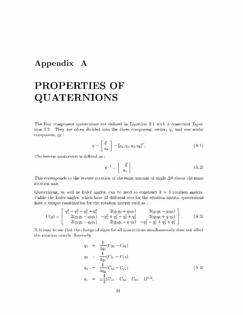
Appendix. A

PROPERTIES OF

QUATERNIONS

The four component quaternions are de�ned in Equation 2.1 with a constraint Equa-tion 2.2. They are often divided into the three component vector, ~q, and one scalarcomponent, q4 :

q =

�~qq4

�= [q1; q2; q3; q4]

T : (A.1)

The inverse quaternion is de�ned as :

q�1 �� �~q

q4

�: (A.2)

This corresponds to the reverse rotation of the same amount of angle �� about the samerotation axis.

Quaternions, as well as Euler angles, can be used to construct 3 � 3 rotation matrix.Unlike the Euler angles, which have 12 di�erent sets for the rotation matrix, quaternionshave a unique combination for the rotation matrix such as :

C(q) =

24 q21 � q22 � q23 + q24 2(q1q2 + q3q4) 2(q1q3 � q2q4)

2(q1q2 � q3q4) �q21 + q22 � q23 + q24 2(q2q3 + q1q4)2(q1q3 + q2q4) 2(q2q3 � q1q4) �q21 � q22 + q23 + q24

35 : (A.3)

It is easy to see that the change of signs for all quaternions simultaneously does not a�ectthe rotation matrix. Inversely,

q1 =1

4q4(C23 � C32)

q2 =1

4q4(C31 � C13)

q3 =1

4q4(C12 � C21) (A.4)

q4 = �1

2(C11 + C22 + C33 + 1)1=2;

91

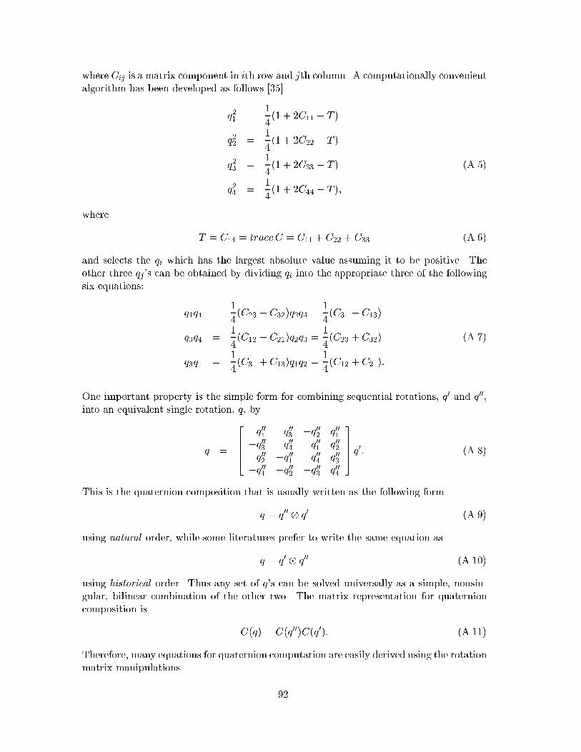
where Cij is a matrix component in ith row and jth column. A computationally convenientalgorithm has been developed as follows [35].

q21 =1

4(1 + 2C11 � T )

q22 =1

4(1 + 2C22 � T )

q23 =1

4(1 + 2C33 � T ) (A.5)

q24 =1

4(1 + 2C44 � T );

where

T = C44 = traceC = C11 + C22 + C33 (A.6)

and selects the qi which has the largest absolute value assuming it to be positive. Theother three qj's can be obtained by dividing qi into the appropriate three of the followingsix equations:

q1q4 =1

4(C23 � C32)q2q4 =

1

4(C31 � C13)

q3q4 =1

4(C12 � C21)q2q3 =

1

4(C23 + C32) (A.7)

q3q1 =1

4(C31 + C13)q1q2 =

1

4(C12 + C21):

One important property is the simple form for combining sequential rotations, q0 and q00,into an equivalent single rotation, q, by

q =

2664

q004 q003 �q002 q001�q003 q004 q001 q002q002 �q001 q004 q003

�q001 �q002 �q003 q004

3775 q0: (A.8)

This is the quaternion composition that is usually written as the following form

q = q00 q0 (A.9)

using natural order, while some literatures prefer to write the same equation as

q = q0 � q00 (A.10)

using historical order. Thus any set of q's can be solved universally as a simple, nonsin-gular, bilinear combination of the other two. The matrix representation for quaternioncomposition is

C(q) = C(q00)C(q0): (A.11)

Therefore, many equations for quaternion computation are easily derived using the rotationmatrix manipulations.

92

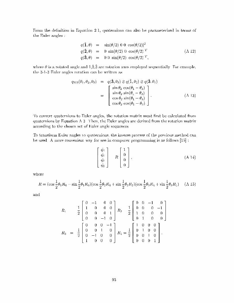
From the de�nition in Equation 2.1, quaternions can also be parameterized in terms ofthe Euler angles :

q(1; �) = [sin(�=2) 0 0 cos(�=2)]T

q(2; �) = [0 sin(�=2) 0 cos(�=2)]T (A.12)

q(3; �) = [0 0 sin(�=2) cos(�=2)]T ;

where � is a rotated angle and 1,2,3 are rotation axes employed sequentially. For example,the 3-1-3 Euler angles rotation can be written as

q313(�1; �2; �3) = q(3; �3) q(1; �2) q(3; �1)

=

2664

sin �2 cos(�1 � �3)sin �2 sin(�1 � �3)cos �2 sin(�1 + �3)cos �2 cos(�1 + �3)

3775 : (A.13)

To convert quaternions to Euler angles, the rotation matrix must �rst be calculated fromquaternions by Equation A.3. Then, the Euler angles are derived from the rotation matrixaccording to the chosen set of Euler angle sequences.

To transform Euler angles to quaternions, the inverse process of the previous method canbe used. A more convenient way for use in computer programming is as follows [15] :2

664_q4_q1_q2_q3

3775 = R

26641000

3775 ; (A.14)

where

R = (cos1

2�1R4 + sin

1

2�1R3)(cos

1

2�2R4 + sin

1

2�2R2)(cos

1

2�3R4 + sin

1

2�3R1) (A.15)

and

R1 =1

2

26640 �1 0 01 0 0 00 0 0 10 0 �1 0

3775R2 =

1

2

26640 0 �1 00 0 0 �11 0 0 00 1 0 0

3775

R3 =1

2

26640 0 0 �10 0 1 00 �1 0 01 0 0 0

3775R4 =

1

2

26641 0 0 00 1 0 00 0 1 00 0 0 1

3775 :

93