TThe Changing Landscapehe Changing Landscape … of geopolitical aggregates is helpful since national or subnational borders help delineate the boundaries of economic, political, and

© 2010 The Shifting Patterns of Agricultural Production and Productivity Worldwide. The Midwest Agribusiness Trade Research and Information Center, Iowa State University, Ames, Iowa.

CHAPTER 2

The Changing LandscapeThe Changing Landscapeof Global Agricultureof Global Agriculture

Jason M. Beddow, Philip G. Pardey, Jawoo Koo, and Stanley Wood

Jason Beddow is a PhD candidate in the Department of Applied Economics at the University of Minnesota. Philip Pardey is a professor in the Department of Applied Economics at the Univer-sity of Minnesota and director of the International Science and Technology Practice and Policy (InSTePP) center. Jawoo Koo is a research fellow and Stanley Wood is a senior research fellow at the International Food Policy Research Institute, Washington, D.C.

The authors are grateful for the assistance of Ulrike Wood-Sichra and Kate Sebastian in processing FAO data, and Michelle Hallaway and Connie Chan-Kang for assisting with entering and cleaning the U.S. data. Zhe “Joe” Guo provided GIS assistance with the global corn, wheat, rice, and soybeans spatial disaggregation. The work for this project was partly supported by the University of Minnesota, the U.S. Agency for International Development, and the Bill and Melinda Gates Foundation.

1. INTRODUCTIONLocation matters when it comes to assessing agricultural productivity levels

and trends. Most fi nd familiarity with the notion that the amount and composi-tion of agricultural output of a particular country or region of the world tends to change over time, but many are less familiar with the spatial dynamics of agricul-ture. The spatial structure and location of agricultural production both between and within countries, which we dub the landscape of agriculture, also varies over time. Agriculture is an inherently spatial process, with yields (and hence out-put) being greatly infl uenced by local factors such as weather and climate, soils, and pest pressures. Consequently, agricultural production and productivity are especially sensitive to spatial and inter-temporal variations in natural factors of production. As we do in this chapter, giving more explicit attention to the spatial dimensions of agriculture and how they change over time deepens our under-

8 BEDDOW, PARDEY, KOO, AND WOOD

standing of the production and productivity performance and potential of this sector. The following section begins by presenting a broad assessment of changes in the global footprint of agriculture over the past three centuries. Agriculture is continually on the move, and this spatial volatility has profound implications for how productivity metrics can and should be interpreted.

Consideration of explicitly spatial patterns is useful, but additional insights can be gained by conducting analyses across meaningful spatial aggregations. Such spatial aggregations summarize certain attributes of space that affect ag-ricultural production and productivity. For example, assessing production in terms of geopolitical aggregates is helpful since national or subnational borders help delineate the boundaries of economic, political, and social factors that affect the production choices made by farmers and other decisionmakers. However, geopolitical boundaries provide a poor proxy for agroecology. Thus, a more com-plete view of agricultural production can be developed by placing production in both geopolitical and agroecological space, as we do in Sections 3 and 4, respec-tively. Since movements in the footprint of agriculture necessarily imply under-lying changes in the natural and socioeconomic factors that drive productivity, thoughtful interpretation of differences in a productivity metric across time or space requires consideration of the extent to which such changes might or might not be captured by that metric. Therefore, these assessments provide grounding and context for the discussions of productivity in the remainder of this volume.

Agricultural statistics are almost always reported on a geopolitical basis, but analysts are increasingly placing agricultural production in agroecological space. Recent examples include the work of Wood, You, and Zhang (2004) and You and Wood (2005) to develop geo-referenced global crop geographies for the world’s principal (food) crops. Ramankutty and Foley (1999) and Ramankutty et al. (2008) have developed long-run geo-referenced maps of the location of crop production worldwide. It is to these sources of data—supplemented with global, commodity-specifi c production data from FAO—that we turn to assess the spatial dynamics of agriculture from both a geopolitical and an agroecological perspective.

2. SPATIAL DYNAMICS OF GLOBAL CROPPED AREAWhile natural inputs play an important, if not defi ning, role in agricultural

production, agriculture is the antithesis of natural. The output and productivity responses to these natural factors are affected by a myriad of human interven-tions. Choices about what, where, and when to grow or graze are obvious infl u-

THE CHANGING LANDSCAPE OF GLOBAL AGRICULTURE 9

ences. Modifying the physical or environmental landscape—from leveling or terracing fi elds to adding fertilizer, supplemental irrigation water, or herbicides and pesticides, all the way to hydroponic production in glasshouse controlled environments—is commonplace. Modifying the genetics of crops and animals is also common.1 For most of the 10,000-year history of agriculture, the purposeful selection and cultivation of crops and animals was without scientifi c direction. The rediscovery of Mendel’s laws of heredity in 1900 gave added impetus to ge-netic modifi cation in agriculture. The commercialization of hybrid corn in the United States beginning in the 1930s and the release of genetically modifi ed (in-cluding transgenic) crops beginning in the 1990s are a continuation of the long history of human-induced genetic modifi cation that is the essence of agriculture. It is the continuously evolving interaction between genes and the environment that underscores the value of a spatially sensitive perspective on agriculture pro-duction processes. The history of this evolution begins with the origins of the crops themselves.

Where crops, or their precursor plants, originated and where they are now principally grown are two sides of the same coin. Identifying the centers of origin of cultivated crops, and even whether such centers exist at all, is subject to considerable debate. Perhaps the most well-known line of reasoning started with the work of Vavilov (1926), who proposed that crops had geographical “centers of origin” and identifi ed eight centers of origin based on measures of diversity. As summarized by Harlan (1971), it was later recognized that the centers of origin may differ from centers of diversity, and further, that the pro-cess of domestication can be geographically dispersed. A big part of the longer history of agricultural innovation has to do with the human-induced spatial movement of plants and animals. Candolle (1884, p. 2) noted that when it is feasible to do so, people “soon adopt certain plants, discovered elsewhere, of which the advantage is evident, and are thereby diverted from the cultivation of the poorer species of their own country.” Further, Candolle observed that the ancient propagation of a number of useful plants in the Mediterranean (by Egyptians and Phoenicians) enabled later migrants to carry West Asian genetic material into Europe at least 4,000 years ago, and that there is evidence of well-established Chinese cultivation of rice, sweet potatoes, wheat, and millets

1The domestication of plants and animals distinguishes agriculture from earlier forms of food production, which involved hunter-gatherer activities whereby humans did not typically manage or in other ways knowingly modify (e.g., genetically) the food sources they sought.


as early as 2,700 BC.2 It is clear that the pre-history of agriculture was driven by human-mediated dispersal and propagation of crop genetic material and therefore that the landscape of agriculture is, and has long been, subject to near continuous change.

Most agricultural production today uses genetic material that had its source hundreds or even thousands of miles away, but this is a comparatively recent phenomenon (Table 2.1). After thousands of years of slow development, slow im-provement, and gradual movement of plants and animals, all driven by human action, the rate of change accelerated in the past 500 years. An important event in this history was the “Colombian Exchange” that was initiated when Colum-bus fi rst made contact with native Americans in the “New World” (Crosby 1987, Diamond 1999). Most of the commercial agriculture in the United States today is based on crop and livestock species introduced from Eurasia (e.g., wheat, barley, rice, soybeans, grapes, apples, citrus, cattle, sheep, hogs, and chickens), though with signifi cant involvement of American species (e.g., corn, peppers, potatoes, tobacco, tomatoes, and turkeys) that are also distributed throughout the rest of the world. The global diffusion of agriculturally signifi cant plants and animals, and their accompanying pests and diseases, has been a pivotal element in the history of agricultural innovation.

The more recent, but still lengthy, spatial history of cropping patterns developed by Ramankutty and Foley (1999) used 1992 satellite-derived land-cover estimates along with historical (geopolitical) crop inventory data and a simple land-cover change model to estimate global cropping patterns back to 1700. Here, we make use of Ramankutty and Foley’s long-run cropping data along with a similar global cropland dataset for 2000 (Ramankutty et al. 2008) to draw conclusions about changes in the geography of agricultural production over the last three centuries. These datasets are distributed by the Center for Sustainability and the Global Environment (SAGE) at the University of Wis-consin and for the sake of brevity will hereafter be referred to as the “SAGE” series (see the appendix).

We used a variety of techniques to represent the changing spatial patterns evident in the SAGE data. Figure 2.1, Panels a and b, give a mapped represen-tation of the SAGE data for 1700 and 2000 respectively. Darker shades indicate that greater percentages of each 55.7-by-55.7 kilometer pixel (projected to the

2In fact, Fuller et al. (2009) recently reported evidence of the domestication of rice in the Lower Yangtze region of Zhejiang that dates to between 6,900 and 6,600 years ago.


Table 2.1. Regions of origin and current production of major feed, food, and fi ber crops Top Five Producing Countries in 2005-07

Crop Center of Origin Country Production

(mmt) Global Share

(percent) Wheat Central Asia China 103.9 17.0 India 71.0 11.6 United States of America 53.4 8.7 Russian Federation 47.4 7.8 France 35.2 5.8 Top Five Total 310.8 50.9Corn South Mexico

and Central America

United States of America 294.0 40.1 China 145.7 19.9 Brazil 43.1 5.9 Mexico 21.2 2.9 Argentina 18.9 2.6 Top Five Total 523.0 71.3Rice India China 184.4 28.7 India 139.3 21.7 Indonesia 55.2 8.6 Bangladesh 42.3 6.6 Viet Nam 35.7 5.6 Top Five Total 456.9 71.1Barley Abyssinia Russian Federation 16.5 12.0 (Ethiopia) Germany 11.5 8.3 Canada 11.0 8.0 France 10.1 7.3 Turkey 8.8 6.4 Top Five Total 58.0 42.0Soybeans China United States of America 80.6 37.0 Brazil 53.9 24.8 Argentina 41.4 19.0 China 15.8 7.3 India 8.9 4.1 Top Five Total 200.6 92.2Cassava South America Nigeria 44.3 20.2 Brazil 26.6 12.1 Thailand 22.0 10.0 Indonesia 19.6 8.9

Congo, Democratic Republic of 15.0 6.8

Top Five Total 127.5 58.1Coffee Abyssinia Brazil 2.3 30.5 (Ethiopia) Viet Nam 0.9 11.8 Colombia 0.7 9.3 Indonesia 0.7 8.7 Mexico 0.3 4.1 Top Five Total 4.8 64.3


Sources: Centers of origin are from Schery’s (1972) adaptation of Vavilov (1951). See the appendix for sources of production shares.

Table 2.1. Continued Top Five Producing Countries in 2005-07

Crop Center of Origin Country Production

(mmt) Global Share

(percent) Bananas Indo-Malaya India 18.1 23.5 China 7.0 9.1 Brazil 6.9 8.9 Philippines 6.7 8.7 Ecuador 6.1 8.0 Top Five Total 44.8 58.3Tomatoes South America China 32.6 25.8 United States of America 11.3 8.9 Turkey 9.9 7.9 India 8.9 7.0 Egypt 7.6 6.0 Top Five Total 70.3 55.6Potatoes South America China 71.1 22.3 Russian Federation 37.5 11.8 India 24.6 7.7 Ukraine 19.3 6.1 United States of America 18.9 5.9 Top Five Total 171.5 53.8Apples Central Asia China 25.9 40.8 United States of America 4.4 6.9 Iran, Islamic Republic of 2.7 4.2 Turkey 2.3 3.6 Italy 2.1 3.4 Top Five Total 37.3 58.9Oranges India Brazil 18.1 28.4 United States of America 8.0 12.6 Mexico 4.1 6.5 India 3.5 5.6 China 2.8 4.4 Top Five Total 36.5 57.5Grapes Central Asia Italy 8.5 12.7 France 6.7 10.0 United States of America 6.3 9.5 Spain 6.2 9.2 China 6.1 9.1 Top Five Total 33.7 50.4Cotton South Mexico

and Central America

China 20.1 28.2 United States of America 12.2 17.1 India 10.2 14.3 Pakistan 6.4 8.9 Uzbekistan 3.5 5.0 Top Five Total 52.3 73.6


Figure 2.1. Panels a and b. The changing global landscape of crop production, 1700 to 2000Source: Derived from SAGE data (see the appendix).

Percentage of AreaUnder Cultivation

0<1010 to 2525 to 5050 to 7575 to 90>90

Panel a: Cropland Extent, 1700

Panel b: Cropland Extent, 2000


Figure 2.1. Panels c and d. The changing global landscape of crop production, 1700 to 2000Source: Derived from SAGE data (see the appendix).

Panel d: Change in Cropland Area, 1960 vs. 2000

600

400

200

0

200

400

600

800

1,000

1,250 750 250 250 750

North AmericaCentral America

South America

Europe

Africa

Asia

Australia 1992 1992

1900

1950

1850

North (km)

South (km)

East

(km

)

Wes

t (km

)

Panel C: Movement of the Regional Centroilds of Cropland, 1700-2000

Change in Share ofLand Under Cultivation

< -0.5-0.5 to -0.25-0.25 to -0.05-0.05 to 0.050.05 to 0.250.25 to 0.5>0.5


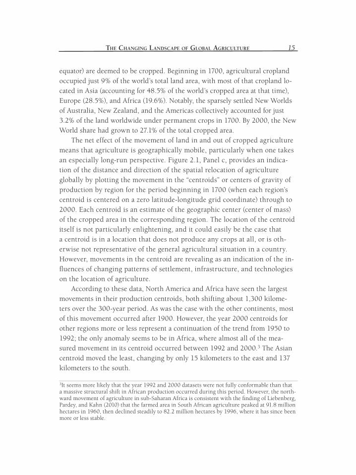
equator) are deemed to be cropped. Beginning in 1700, agricultural cropland occupied just 9% of the world’s total land area, with most of that cropland lo-cated in Asia (accounting for 48.5% of the world’s cropped area at that time), Europe (28.5%), and Africa (19.6%). Notably, the sparsely settled New Worlds of Australia, New Zealand, and the Americas collectively accounted for just 3.2% of the land worldwide under permanent crops in 1700. By 2000, the New World share had grown to 27.1% of the total cropped area.

The net effect of the movement of land in and out of cropped agriculture means that agriculture is geographically mobile, particularly when one takes an especially long-run perspective. Figure 2.1, Panel c, provides an indica-tion of the distance and direction of the spatial relocation of agriculture globally by plotting the movement in the “centroids” or centers of gravity of production by region for the period beginning in 1700 (when each region’s centroid is centered on a zero latitude-longitude grid coordinate) through to 2000. Each centroid is an estimate of the geographic center (center of mass) of the cropped area in the corresponding region. The location of the centroid itself is not particularly enlightening, and it could easily be the case that a centroid is in a location that does not produce any crops at all, or is oth-erwise not representative of the general agricultural situation in a country. However, movements in the centroid are revealing as an indication of the in-fl uences of changing patterns of settlement, infrastructure, and technologies on the location of agriculture.

According to these data, North America and Africa have seen the largest movements in their production centroids, both shifting about 1,300 kilome-ters over the 300-year period. As was the case with the other continents, most of this movement occurred after 1900. However, the year 2000 centroids for other regions more or less represent a continuation of the trend from 1950 to 1992; the only anomaly seems to be in Africa, where almost all of the mea-sured movement in its centroid occurred between 1992 and 2000.3 The Asian centroid moved the least, changing by only 15 kilometers to the east and 137 kilometers to the south.

3It seems more likely that the year 1992 and 2000 datasets were not fully conformable than that a massive structural shift in African production occurred during this period. However, the north-ward movement of agriculture in sub-Saharan Africa is consistent with the fi nding of Liebenberg, Pardey, and Kahn (2010) that the farmed area in South African agriculture peaked at 91.8 million hectares in 1960, then declined steadily to 82.2 million hectares by 1996, where it has since been more or less stable.


Except in Africa and Asia, the general trend favored movement in longi-tude rather than latitude. The pronounced northward movement in Africa was almost matched by an equivalent move westward, and, while the Asian cen-troid showed much more absolute movement along the east-west axis, the net movement over the period was almost due south. Averaging across all of the regions, the net longitudinal movement was 4.6 times as large as the net lati-tudinal movement. This pattern is related to an argument by Diamond (1999, p. 185), who stated that “localities distributed east and west of each other at the same latitude share exactly the same day length and its seasonal varia-tions. To a lesser degree, they also tend to share similar diseases, regimes of temperature and rainfall, and habitats or biomes (types of vegetation).” Thus, a variety that is successful at a given location is more likely to be successful at other locations with similar latitude, and therefore a spread along the east-west axis is easier than a spread along the north-south axis.4 This argument provides insights into the forces underlying the direction of agricultural move-ments, although the implications for modern movements in overall production are less clear. For example, opposite latitudinal movements in different crops may be netted out of an assessment of overall production. Second, Diamond took a very long-run view, looking back to pre-history. Insofar as crop manage-ment and varietal improvement technologies are reducing the yield-depressing effects of constraints to agricultural production at the more extreme latitudes, one might expect more recent data to exhibit relatively more movement toward the poles.

Over the past three centuries, agricultural cropland in Asia and Europe did move along an east-west axis, but there was considerable movement along a north-south axis as well. In addition, the direction of Eurasian development changed course. European cropland moved in a northeasterly direction until the early 1990s, then took a U-turn, heading southwesterly during the 1990s, no doubt the consequence of an implosion in Soviet agriculture during this period (see Swinnen and Van Herck in Chapter 10 of this volume). Asia moved simi-

4Diamond couched his discussion in the context of social developments stretching back into pre-history. Our assessment of the spatial mobility of cropped agriculture begins in 1700. Develop-ments after 1700 dominate the economic landscape. For example, Maddison (2003) reports that global population was just 603 million in 1700 compared with 6.1 billion in 2001, while global GDP grew from an estimated 371 billion in 1700 to 37 trillion in 2000 (in constant 1990 interna-tional dollars). Moreover, most of the increase in the area under crops occurred after 1700, with global cropped area expanding by an estimated 253% since then (from 422 million hectares in 1700 to 1.49 billion hectares in 2000 [Ramankutty and Foley 1999 and Ramankutty et al. 2008]).


larly, following a northeasterly trajectory until the 1850s, and then also took a southwesterly track. As of 2000, the Asian centroid was in north-central Bhutan near the border within China, suggesting that the relative rates and spatial pat-terns of cropland development in China and India dominate the movement in the region’s centroid. However, expanding cropland in Indochina and Indonesia during the latter half of the nineteenth century and throughout the twentieth century would tend to tug Asia’s centroid southward.

As one might expect given the way these landscapes were settled (particu-larly with regard to agriculture), both the North American and Australian cen-troids moved strongly in a westerly direction. This westward movement came with an evident northerly drift that became more pronounced for North America beginning in 1900 and in 1950 for Australia. Notably, a more northerly direc-tion of development for North American agriculture means cooler climates and shorter growing seasons while for Australia it means movement toward more tropical growing conditions. The more northerly path taken by North American agriculture during the twentieth century coincides with the massive ramping up of institutions and investments pertaining to agricultural research and develop-ment (see Alston et al. 2010), suggesting that technological factors began playing a more prominent role in the location of crop production.5 The same forces may have also been operative in Australia, with increasing attention given to tropical technologies by Australian agricultural research institutions during the twentieth century, overlaid with (and part of) a broader government-sponsored program of infrastructure and economic development that put greater emphasis on the more northerly parts of the country (Davidson 1966 and 1981).

Cropland in Central America6 shifted northwesterly, as developments in Mexico increasingly dominated that landscape. In stark contrast, South American cropland moved strongly in a southerly direction from 1700 to the 1950s, then dramatically changed course, heading northeast for much of the latter half of the twentieth century as Brazilian agriculture occupied

5Settlement patterns and the importation of cold-tolerant varieties help to explain the northerly movement of North American agriculture during the nineteenth century. Twentieth century ex-pansion was much less dependent on opening of new lands and importation of germplasm, and much more dependent on the homegrown development and uptake of new corn varieties, notably the rapid uptake of short-duration hybrid varieties beginning in the 1930s that allowed for more intense production, and that spurred a movement into more northerly areas. 6Central America is typically defi ned as the area of Belize, Costa Rica, El Salvador, Guatemala, Honduras, Nicaragua, and Panama. We also include Mexico because of its climatic and agricultural-historical similarities with the Central American countries.


an increasing share of the region’s cropland (an estimated 25.3% in 1950 and 46.7% in 2000). As in Australia, the South American reversal of direc-tion may stem largely from technological and economic policy developments in Brazil. The country rapidly ramped up its agricultural research capacity during the latter half of the twentieth century (Beintema, Avila, and Pardey 2001), and increasingly targeted that effort to more northerly climes. Spill-over technologies from other countries—most notably day-length insensitive soybean varieties developed in the United States (Pardey et al. 2006)—en-abled large tracts of land to be opened up for agriculture in the Cerrados region of Brazil. These technological factors were reinforced by a series of national development strategies that also targeted more northerly regions of the country.

Panel d of Figure 2.1 uses the SAGE series to show the change in cropped area over the four decades spanning 1960 to 2000. It indicates the localized movement of acreage in and out of agriculture since 1960, or, more specifi -cally, the change in the area share dedicated to crop production for each of the 259,200 mapped pixels (i.e., a value of -50% indicates that half the acre-age in that pixel shifted out of cropping agriculture since 1960). The darker the red shading, the greater the percent decline in cropped area per pixel; the darker the green shading, the greater the percent increase in cropped area per pixel. The collapse of the former Soviet Union is evident in terms of substan-tial declines in cropped area throughout Eastern Europe. The SAGE data also indicate declines in cropped area in parts of Western Europe, northeastern, southern, and southeastern United States, and signifi cant parts of China.7 There was a substantial increase in cropped areas throughout the Indochina Peninsula, Indonesia, West Africa, Mexico, and Brazil. The overall picture is one of contracting area under crops in temperate regions and increasing cropped area in tropical parts of the world during the last four decades of the twentieth century.

While the centroid of production provides a sense of the “average” location of production for a region, it is also useful to characterize the spatial disper-sion of production. One can summarize spatial dispersion in a variety of ways,

7Wood, Sebastian, and Scherr (2000, p. 28) document the reduction in cultivated land in China during the fi rst half of the 1990s, largely attributing this to expanded industrial and urban uses of land. Zhang et al. (2007) imply that this trend continued into at least the early part of the twenty-fi rst century. For example, the authors estimate that 260,000 hectares of Chinese culti-vated land was converted to non-agricultural uses between 1991 and 2001.


most commonly by assessing whether observations seem to be correlated with other nearby observations by calculating test statistics such as Moran’s I (Moran 1950) and Geary’s C (Geary 1954) metric.8 In the present case, these statistics were calculated for each region in each year and the null hypothesis of spatial homogeneity was rejected for any reasonable degree of certainty, confi rming the common-sense expectation that agriculture was not distributed uniformly across any of the continents.9

For our purposes, it is perhaps more useful to consider metrics of dispersion that are not explicitly spatial. Economists often analyze income distributions using a methodology fi rst described by Lorenz (1905), who graphed cumula-tive income distribution against population percentiles. If income were equally distributed among the population, the Lorenz curve would be a 45-degree line through the origin, and the degree to which the curve departs from that line is usually summarized by the Gini coeffi cient (Gini 1912). Here, we make use of the pixilated landscape (30 arc-minute or 5 arc-minute pixels) inherent in the SAGE series and use Gini’s procedure to assess the degree to which crop produc-tion is concentrated within each region.10

In this spatial context, the calculated Gini coeffi cients will equal zero if each of a region’s pixels contains the same share of the region’s agricultural area; the value of the coeffi cients will increase as agriculture becomes more concentrated in fewer pixels, and a coeffi cient of unity indicates that all production is in a single pixel.11 In general, Gini coeffi cients differ more across regions than within regions over time. In every period, crop production was most spatially concen-trated in North America and Australia and was least concentrated in Asia and Central America (Table 2.2). The relatively high coeffi cients for North America and Australia refl ect a relatively low ratio of arable to total land, while the low Central American coeffi cients refl ect the opposite, along with a tendency for

8Indeed, it is generally assumed that spatial autocorrelation is present unless there is evidence to the contrary. For example, the “fi rst law of geography” states “Everything is related to everything else, but near things are more related than distant things” (Tobler 1970, p. 236). 9To reduce the scope of the problem, the spatial weights required for the calculations were defi ned using rook contiguity rather than an inverse distance metric. In general, these yield similar results but can differ, especially if production tends to exhibit more global autocorrelation than local autocorrelation. This does not affect the present conclusion.10A 5 arc-minute grid yields pixels (cells) that are of about 86 square kilometers at the equator.11Technically, the Gini coeffi cient calculated over discrete units (e.g., grid cells) cannot equal one; however, under perfect inequality the Gini coeffi cient approaches unity as the number of units approaches infi nity.


relatively non-intensive production. Over time, the Gini coeffi cients for Africa and Central America were stable, while those for the other regions refl ected a decreasing spatial concentration of production, as the agricultural footprint of these areas expanded.

Table 2.2 also displays production quartiles which, as implied by the rela-tively stable Gini coeffi cients, are also fairly stable over time. The third quartile shows the percentage of the region’s total land area that contains 75% of the crop area. By this measure, the largest changes occurred in North America, which concentrated three-quarters of its cropped area in only 4.5% of its land area in 1800. By 2000, 9.6% of the region’s land area constituted the same portion of overall cropped area. However, the increased (but still rather concentrated) spa-tial dispersion of cropped area in North America is a special case, as the interior of the continent, which is generally favorable for agricultural production, was not heavily settled until after 1800. By contrast, Central American and Asian production remained relatively spatially dispersed over the entire period, while South American, European, and African agriculture all became more concen-trated after 1900.

3. SPATIAL DYNAMICS OF GLOBAL CROP PRODUCTIONThe previous section explored the long-run, spatially explicit view of agri-

cultural change provided by Ramankutty and Foley (1999) and Ramankutty et al. (2008). We now turn to alternative empirical views of global production for more recent decades by fi rst exploring the commodity- and country-specifi c data

Table 2.2. Spatial dispersion of production by year and region

Sources: See the appendix.Note: The third quartile shows the percentage of each region’s total area accounting for one-quarter of cropland.

Gini Coefficient 3rd Quartile

Region 1800 1900 2000 1800 1900 2000

North America 0.94 0.88 0.87 4.54 8.71 9.56

Central America 0.68 0.68 0.68 24.77 24.77 25.05

South America 0.77 0.75 0.73 18.17 18.73 13.33

Europe 0.80 0.78 0.76 16.07 16.72 11.47

Africa 0.78 0.78 0.79 16.11 15.99 13.21

Asia 0.75 0.74 0.70 18.41 19.72 20.63

Australia 0.93 0.93 0.90 5.37 5.52 4.96


assembled by FAO. These data enable a crop-level assessment of the changing landscape of production within and among countries. Throughout the section, simple economic concepts are employed to provide additional insights that could not otherwise be gleaned from a geopolitical assessment, namely, by considering the interactions between geography, economic development (as measured by in-come per person), and crop values.

3.1. Global Changes in What Is ProducedSince 1961, a large area has been devoted to the production of cereal crops

worldwide, increasing from about 648 million harvested hectares in 1961 to about 700 million hectares in 2007 (roughly 5.6% of the world’s ice-free land area, and 55.8% of global harvested hectares).12 In 2007, oil crops (such as soy-beans and rapeseed) had the second-largest physical footprint, with harvested area for these crops totaling around 250 million hectares—more than double the 113 million hectares of oil crops that were harvested in 1961. Over half (52%) of the increased area in oil crops refl ects a nearly fourfold increase in the area devoted to soybeans. Table 2.3 shows the trends in area devoted to each of the major crop categories used by FAO. Notably, while area devoted to production of oil crops increased steadily over the period, the area under cereals production increased to a maximum of about 720 million hectares by 1985, then generally decreased until an increasing trend again took hold during the new millennium.

Category

Area (million ha) and Trend

1961 Trend 2007

Fiber 38.7 35.8

Fruits 24.5 47.1

Oil crops 113.4 250.5

Pulses 64.0 73.3

Root crops 47.6 54.6

Vegetables 23.7 52.4

Cereals 648.0 699.8

Table 2.3. Global harvested area by crop category

Sources: See the appendix.

12This value was calculated based on Ramankutty et al. (2008), who reported that 15 million km2 of cropland accounted for about 12% of the total ice-free land area in 2000 (which implies that there are roughly 125 million km2 of ice-free land area).


Further, the total area devoted to pulses, fi ber crops, and root crops was little changed, while the areas under fruit and vegetable crops both increased fairly rapidly (with the latter increasing at an increasing rate).

While the land area under cereal production increased from 1961 to 2007, total harvested area over all crops increased even more, so the share of land de-voted to cereal production shrank from 67.5% in 1961 to 57.7% in 2007. This was a widespread development, such that the harvested area dedicated to cereals decreased relative to other crop categories in every region of the world except Eastern Europe. The largest changes were in Latin America and North America, which reduced the share of their cropland devoted to cereals by 17.6 and 14.0 percentage points, respectively (Table 2.4). Offsetting this reduction, the same two regions devoted relatively more of their land to oil crops, and in both re-gions nearly all of the increase in land devoted to oil crops is accounted for by increased soybean production.

3.2. Changes in Where Crops Are Produced Changes in the global crop mix have been accompanied by changes in the

distribution of production among and within countries and regions. Over the past four and a half decades, global cereal output became increasingly concen-trated in Asia. This region increased its share of global cereal production from 37.6% in 1961 to 47.2% by 2007, most of which resulted from relatively fast growth of wheat and corn production in China.13 Over the same period, North American output of cereals grew at about the global average rate, while output in the Former Soviet Union and Europe increased at a slower-than-average rate (2.0%, 0.6%, and 1.4% per year, respectively). Similar patterns were seen for

13Here the aggregate production of cereals, fi ber crops, fruits, vegetables, roots, and pulses is a simple sum of the quantity of production (by weight) of each crop in a particular crop category. This measure of the aggregate quantity of production is affected by changes in the composition of the aggregate, with subtle but substantive implications for assessing changes in crop produc-tivity (and, notably, aggregate cereal yields). For example, average wheat yields in Minnesota in 2007 were 3.0 tons per hectare while corn yielded 9.8 tons per hectare on average. Forming a “total cereals” perspective by simply summing 10 hectares of wheat output (by weight) and 10 hectares of corn output (by weight) would imply a cereal yield of 6.4 tons per hectare. If all the wheat acreage were switched to corn, estimated cereal yields would increase to 9.8 tons per hectare, absent any change in the average yield of corn (or wheat). These compositional effects will confound efforts to interpret changes in measures of aggregate crop productivity when the aggregate quantities of crop output are formed by simply summing the components of the ag-gregate (as done by FAO and many other analysts). Alston et al. (2010) explore the empirical implications of alternative aggregation methods when analyzing productivity developments in twentieth century U.S. agriculture.


other types of crops, with Asia increasing its share of fi ber, fruit, and vegetable production, again refl ecting large increases in Chinese production of these types of commodities (Table 2.5).

In addition to considering geopolitical boundaries, it is also useful to delin-eate the agricultural landscape according to economic factors. To get a sense of how economic development is related to agricultural production, we grouped countries into two categories, “lower income” and “upper income,” according to their income per person.14 Between 1961 and 2007, the lower-income countries increased their share of production of all types of crops except oil crops. These

14The World Bank (2009) classifi es countries according to their 2008 per capita gross national in-come expressed in U.S. dollars. The income groups are high income, greater than $11,905; upper-middle income, $3,856-$11,905; lower-middle income, $976-$3,855; and low income, less than $976. To simplify the presentation, we group the low and lower-middle income countries into one category called “lower income” and the upper-middle and high income countries into a second aggregate called “upper income.” It may be helpful to keep in mind that the upper-income group includes Brazil and Russia while China and India are included in the lower-income group.


Table 2.4. Share of cropland devoted to various crop types, by region

Region Year Fiber Fruits Vegetables Roots Pulses Oil

Crops Cereals (percentage)

North America

1961 5.6 1.0 1.4 0.7 0.7 18.0 72.5

2007 3.2 0.9 1.1 0.5 2.6 33.3 58.5 Latin America and Caribbean

1961 7.2 3.6 2.2 5.2 9.2 13.7 58.9

2007 1.7 5.2 2.1 3.7 6.4 39.5 41.4

Europe 1961 1.0 7.7 4.0 8.3 6.6 3.9 68.4 2007 0.6 7.6 3.3 2.6 1.7 18.0 66.2

Former Soviet Union

1961 2.8 1.2 1.3 6.0 2.9 6.4 79.4

2007 2.5 1.9 2.0 5.0 1.8 13.9 72.9

Africa 1961 4.5 4.3 2.0 8.3 7.1 16.8 57.1 2007 2.6 4.5 2.9 12.0 10.5 13.7 53.9

Asia 1961 4.3 1.6 3.0 4.1 9.3 12.8 65.0 2007 3.9 4.0 6.9 3.3 6.9 18.2 56.8

Oceania 1961 0.2 2.2 1.0 2.0 0.4 4.4 89.8 2007 0.6 1.8 0.7 1.2 6.0 7.8 81.9

World 1961 4.0 2.6 2.5 5.0 6.7 11.8 67.5 2007 3.0 3.9 4.3 4.5 6.0 20.6 57.7


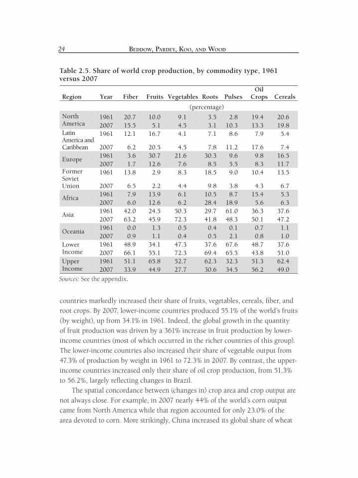
countries markedly increased their share of fruits, vegetables, cereals, fi ber, and root crops. By 2007, lower-income countries produced 55.1% of the world’s fruits (by weight), up from 34.1% in 1961. Indeed, the global growth in the quantity of fruit production was driven by a 361% increase in fruit production by lower-income countries (most of which occurred in the richer countries of this group). The lower-income countries also increased their share of vegetable output from 47.3% of production by weight in 1961 to 72.3% in 2007. By contrast, the upper-income countries increased only their share of oil crop production, from 51.3% to 56.2%, largely refl ecting changes in Brazil.

The spatial concordance between (changes in) crop area and crop output are not always close. For example, in 2007 nearly 44% of the world’s corn output came from North America while that region accounted for only 23.0% of the area devoted to corn. More strikingly, China increased its global share of wheat

Table 2.5. Share of world crop production, by commodity type, 1961 versus 2007



Crops Cereals (percentage)

North America

1961 20.7 10.0 9.1 3.5 2.8 19.4 20.6 2007 15.5 5.1 4.5 3.1 10.3 13.3 19.8

Latin America and Caribbean

1961 12.1 16.7 4.1 7.1 8.6 7.9 5.4

2007 6.2 20.5 4.5 7.8 11.2 17.6 7.4

Europe 1961 3.6 30.7 21.6 30.3 9.6 9.8 16.5 2007 1.7 12.6 7.6 8.5 5.5 8.3 11.7

Former Soviet Union

1961 13.8 2.9 8.3 18.5 9.0 10.4 13.5

2007 6.5 2.2 4.4 9.8 3.8 4.3 6.7

Africa 1961 7.9 13.9 6.1 10.5 8.7 15.4 5.3 2007 6.0 12.6 6.2 28.4 18.9 5.6 6.3

Asia 1961 42.0 24.5 50.3 29.7 61.0 36.3 37.6 2007 63.2 45.9 72.3 41.8 48.3 50.1 47.2

Oceania 1961 0.0 1.3 0.5 0.4 0.1 0.7 1.1 2007 0.9 1.1 0.4 0.5 2.1 0.8 1.0

Lower Income

1961 48.9 34.1 47.3 37.6 67.6 48.7 37.6 2007 66.1 55.1 72.3 69.4 65.5 43.8 51.0

Upper Income

1961 51.1 65.8 52.7 62.3 32.3 51.3 62.4 2007 33.9 44.9 27.7 30.6 34.5 56.2 49.0


production from 6.4% in 1961 to 18.1% in 2007, while its share of land devoted to wheat shrank slightly. Such differences in output and area shares refl ect differ-ences in average yields (land productivity) across regions. They also reinforce the fi ndings previously mentioned of the substantial spatial relocation in cropped area worldwide, pointing to even greater movement in the location of production for specifi c crops both among and within countries. This movement has many important economic implications, not least in relation to understanding the fun-damental forces driving observed changes in (aggregate) crop production and productivity estimates.15

Between 1961 and 2007, the world’s fruit and vegetable production area be-came more concentrated in Asia and, to a lesser extent, Africa (Table 2.6). Asia now accounts for 45.5% of the land devoted to fruit production and 71.5% of the

15A more in-depth assessment of productivity developments worldwide and in specifi c countries is provided in the following chapters.

Table 2.6. Share of world crop area, by commodity type, 1961 versus 2007



Crops Cereals (percentage) North America

1961 16.4 4.8 6.5 1.7 1.3 17.9 12.6 2007 11.9 2.6 2.7 1.2 4.7 17.8 11.2


1961 11.8 9.2 5.8 7.0 9.1 7.6 5.8

2007 5.8 13.4 4.9 8.1 10.5 19.1 7.1

Europe 1961 2.8 33.7 18.1 18.7 11.1 3.7 11.3 2007 1.4 14.3 5.6 4.3 2.1 6.4 8.4

Former Soviet Union

1961 10.8 7.0 8.3 18.7 6.7 8.4 18.2

2007 7.8 4.7 4.4 10.4 2.7 6.2 11.7

Africa 1961 11.6 17.7 8.4 17.4 11.1 14.8 8.8 2007 14.0 18.7 10.6 42.8 27.7 10.6 15.0

Asia 1961 46.6 26.8 52.4 36.2 60.6 47.1 42.0 2007 58.7 45.5 71.5 32.8 50.5 39.2 43.9

Oceania 1961 0.0 0.8 0.4 0.4 0.1 0.4 1.3 2007 0.4 0.9 0.3 0.5 1.9 0.7 2.7

Lower Income

1961 56.9 37.2 55.1 52.4 70.7 59.7 46.6 2007 71.6 60.4 78.2 76.1 77.4 48.8 56.0

Upper Income

1961 43.1 62.8 44.8 47.5 29.3 40.3 53.4 2007 28.4 39.6 21.7 23.8 22.5 51.2 44.0


land devoted to vegetable production, versus 26.8% and 52.4% in 1961, respec-tively. This change resulted mostly from increases in Asian fruit production area rather than from decreases elsewhere. Europe’s fruit area decreased by 18.5% overall over the period, the net result of a 30.5% decrease in Western Europe and a 62.3% increase in Eastern Europe.

Over the same period, Asia increased its vegetable production area by a remarkable 202.4%. Increased vegetable area in China (18.3 million additional hectares) contributed to this change, although Asia without China still more than doubled its land devoted to vegetable production. A similar percentage in-crease in vegetable land area was seen in Africa (179.2%), although the continent only managed to keep pace with worldwide increases, maintaining a global share of production of slightly more than 6% during both periods.

3.3. Global Crop Production: An Economic View In the preceding analyses, the crop categories used to describe changes in

the cropped areas and amounts produced were based on quantities (by weight) of crop production aggregated into standard crop categories conceived on the ba-sis of the biology of each crop (e.g., cereals, fruits, root crops, and so on). In this section we re-aggregate the crop quantities into crop categories conceived on the basis of the per unit value of each crop.

To conduct our analysis of the shifting landscape of crops grouped on eco-nomic criteria, all 157 crops (and crop products) in the FAO database (FAOSTAT) were classifi ed into three groups, low, medium, and high unit-valued crops ac-cording to their average international price during 1999-2001 as reported by Wood-Sichra (2005).16 Crop values ranged from about $20 per metric ton for sugarcane to nearly $4,500 per metric ton for vanilla. Acreage in low unit-valued crops is dominated by the cereals (wheat, corn, rice, and barley) and soybeans, which account for about 70% of the area in low-value crops. The most important high unit-valued crops (by area) were cotton, coffee, sesame seeds, cocoa, tobacco, and tea while the acreage in medium unit-valued crops was dominated by com-modities such as dry beans, various peas, pulses, groundnuts, and olives.

16Prices reported by Wood-Sichra are the 1999-2001 average international prices used by FAO to form their production indices (see http://faostat.fao.org/site/612/default.aspx). Crops with an average price greater than $700 per metric ton were classifi ed as high-value crops, while those with prices under $250 per metric ton were classifi ed as low-value crops. Most livestock products would fall in the high-valued class, but here we limit our analysis to a consideration of plant products (not least because area under production is a more straightforward concept for crops versus livestock production).


Between 1961 and 2007, the global share of total cropped area devoted to low- and high-value crop production increased by about the same percent-age, 24.2% and 28.5%, respectively. Over the same period, the area devoted to medium-value commodities increased by 68.8% (Table 2.7). Thus, there was a slight shift toward production of medium-value crops, and that shift was evident in both lower- and upper-income countries. However, the nature of the change was different for different types of countries: the importance of medium-value crops increased in the upper-income countries in part be-cause of reductions in high-value crop area, while lower-income countries increased the area of all three classes of crops. This analysis reveals that the decline in harvested area in the Former Soviet Union and Europe resulted from decreases in area under low-value crops (by 38.9 and 20.7 million hect-ares, respectively) combined with small increases in the area under medium-

Table 2.7. Area by crop value class and region, 1961 and 2007


Region Year Value Class

Low Medium High (million ha)

North America 1961 97.4 3.3 7.2 2007 115.6 10.4 5.2


1961 51.3 7.9 13.2 2007 115.1 12.1 10.6

Europe 1961 91.2 16.5 2.1 2007 70.5 19.1 2.2

Former Soviet Union

1961 142.7 4.3 2.6 2007 103.8 5.0 3.1

Asia 1961 333.6 58.7 24.4 2007 421.1 95.1 39.6

Africa 1961 76.5 16.0 11.3 2007 149.1 36.8 17.1

Oceania 1961 9.7 0.2 0.1 2007 21.5 2.0 0.4

World Total 1961 802.9 106.9 60.9 2007 996.4 180.4 78.2

Lower Income 1961 380.3 70.0 35.2 2007 548.5 126.2 56.6

Upper Income 1961 422.6 36.9 25.7 2007 448.0 54.2 21.6


and high-value commodities. Nevertheless, low-value crop area increased overall because of substantial increases in every other region.

4. AN AGROCLIMATIC PERSPECTIVE ON CROP LANDSCAPESThe spatial lens through which we have examined patterns of agricul-

tural production is explicitly geopolitical. Both the national and subnational production data that underpin our analysis are collected and reported accord-ing to administrative (geopolitical) boundaries that, while not arbitrary, are demarked with little or no consideration of the agroecological variation that directly affects crop location choices and the production and productivity po-tentials of these crops. Thus, considering crop production totals aggregated over geopolitical space masks signifi cant spatial heterogeneity within these ag-gregates that can have important policy and practical consequences.

To illustrate this issue, consider two countries: country A has spatially uniform growing conditions for its 200,000 hectares of rain-fed corn that each yield around 1.5 tons per hectare, while country B contains large extents of more arid areas where 160,000 hectares of production yield a meager 700 kg per hectare under rain-fed production and other more-favored areas where around 40,000 hectares yield 4.7 tons per hectare under irrigation. Both coun-tries report identical national corn production statistics: 200,000 hectares of corn averaging around 1.5 tons per hectare (Table 2.8, Panel a). While the reported corn yields for both countries are identical, this masks the spatial heterogeneity inherent in these geopolitical aggregates, thereby compromising efforts to understand the factors that affect productive performance and varia-tions in productivity over time and among countries.

For example, consider two adjacent countries that equally share 400,000 hectares of corn across a well-watered plain cut by national boundaries that yield some 2 tons per hectare. Additionally one has a further 200,000 hect-ares under dryland conditions yielding 800 kg per hectare, while the second has some 50,000 hectares of land under irrigation yielding 5 tons per hect-are. When presented as national aggregates, their respective average yields of 1.4 tons per hectare and 2.6 tons per hectare suggest quite different pro-duction contexts (with perhaps little scope for technology spillover between these two countries) (Panel b of Table 2.8). Yet the common agroecological domain they share is the largest single productive resource, and so the pro-ductivity potentials of the two countries have much more in common than


would be inferred from a consideration of yield relativities absent the agro-ecological information.

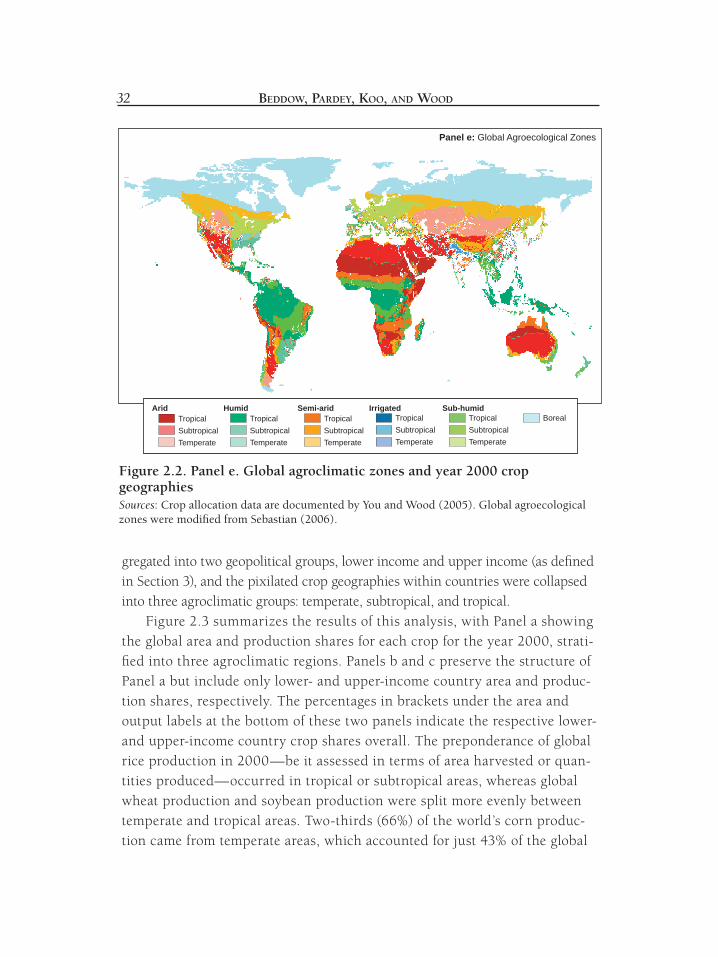
Panels a through d of Figure 2.2 show the year 2000 estimates of the global crop geographies for corn, wheat, rice, and soybeans, respectively. In these plots, the larger the share of cropped area per pixel in the indicated crop, the darker the shade. Panel e of Figure 2.2 shows 16 agroecological zones based on moisture and temperature. To reveal some of the within-country variation in the produc-tion landscape of agriculture, we overlaid the agroclimatic representation on the respective 2000 global crop geographies for corn, wheat, rice, and soybeans to generate production area and quantity estimates for these four crops stratifi ed by agroclimatic regions within countries. For each crop this generated a spatial re-grouping of the area and quantity data for a total of 785 agroclimatic-by-country classifi cations. To simplify the presentation of these data, the countries were re-ag-

Table 2.8. Spatial aggregation bias: geopolitical versus agroecological units

Source: Developed by the authors.

Geopolitical Aggregation Agroecological

Aggregation Implications

Panel a

Country A: 200,000 ha, 1.5 ton ha-1 Country B: 200,000 ha, 1.5 ton ha-1

Country A: Warm, wet lowlands – 200,000 ha, 1.5 ton ha-1 Country B: Hot, semi-arid, poor soils – 160,000 ha, 700 kg ha-1 Hot, irrigated, good soils – 40,000 ha, 4.7 ton ha-1

Geopolitical aggregations infer similar production contexts. Agroecological aggregations reveal large differences.

Panel b

Country A: 400,000 ha, 1.4 ton ha-1

Country B: 250,000 ha, 2.6 ton ha-1

Country A: Warm, wet plains—200,000 ha, 2 ton ha-1 Hot, semi-arid— 200,000 ha, 800 kg ha-1 Country B: Warm, wet plains—200,000 ha, 2 ton ha-1 Warm, irrigated, good soils—50,000 ha, 5 ton ha-1

Geopolitical aggregations infer dissimilar production contexts. Agroecological aggregations reveal extensive commonalities.


Figure 2.2. Panels a and b. Global agroclimatic zones and year 2000 crop geographies Sources: Crop allocation data are documented by You and Wood (2005). Global agroecological zones were modifi ed from Sebastian (2006).

Panel a: SPAM Modeled Wheat Distribution, 2000

Panel b: SPAM Modeled Rice Distribution, 2000

Thousand Ha. perGrid Cell

0<2020 to 4040 to 7070 to 110110 to 180>180


Figure 2.2. Panels c and d. Global agroclimatic zones and year 2000 crop geographies Sources: Crop allocation data are documented by You and Wood (2005). Global agroecological zones were modifi ed from Sebastian (2006).

Panel c: SPAM ModeledCorn Distribution, 2000

Panel d: SPAM ModeledSoybean Distribution, 2000

Thousand Ha. perGrid Cell

0<2020 to 4040 to 7070 to 110110 to 180>180


Figure 2.2. Panel e. Global agroclimatic zones and year 2000 crop geographies Sources: Crop allocation data are documented by You and Wood (2005). Global agroecological zones were modifi ed from Sebastian (2006).

gregated into two geopolitical groups, lower income and upper income (as defi ned in Section 3), and the pixilated crop geographies within countries were collapsed into three agroclimatic groups: temperate, subtropical, and tropical.

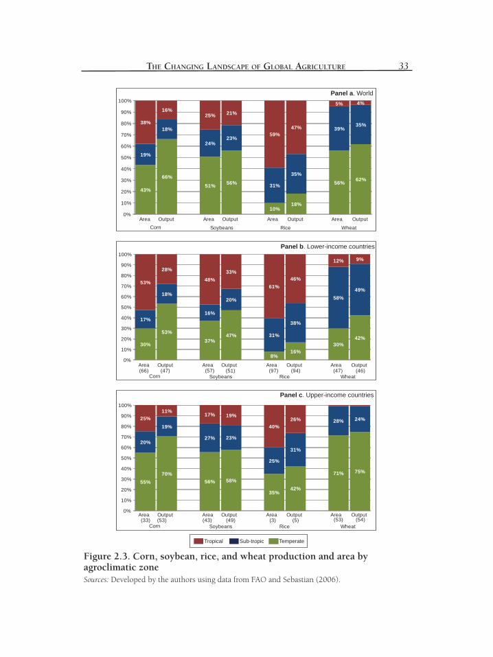
Figure 2.3 summarizes the results of this analysis, with Panel a showing the global area and production shares for each crop for the year 2000, strati-fi ed into three agroclimatic regions. Panels b and c preserve the structure of Panel a but include only lower- and upper-income country area and produc-tion shares, respectively. The percentages in brackets under the area and output labels at the bottom of these two panels indicate the respective lower- and upper-income country crop shares overall. The preponderance of global rice production in 2000—be it assessed in terms of area harvested or quan-tities produced—occurred in tropical or subtropical areas, whereas global wheat production and soybean production were split more evenly between temperate and tropical areas. Two-thirds (66%) of the world’s corn produc-tion came from temperate areas, which accounted for just 43% of the global

Panel e: Global Agroecological Zones

AridTropicalSubtropicalTemperate

BorealTropicalSubtropicalTemperate

Semi-aridTropicalSubtropicalTemperate

Sub-humidTropicalSubtropicalTemperate

HumidTropicalSubtropicalTemperate

Irrigated


Figure 2.3. Corn, soybean, rice, and wheat production and area by agroclimatic zoneSources: Developed by the authors using data from FAO and Sebastian (2006).

Tropical Sub-tropic Temperate

43%51%

10%

56%

19%

24%

31%

39%38%

25%

59%

5%

66%56%

18%

62%

18%

23%

35%

35%

16% 21%

47%

4%

0%

10%

20%

30%

40%

50%

60%

70%

80%

90%

100%

Area OutputCorn Soybeans Rice Wheat

Area Area Area OutputOutputOutput

30%37%

8%

30%

17%16%

31%

58%

53% 48%61%

12%

53% 47%

16%

42%

18%20%

38%

49%

28% 33%46%

9%

0%

10%

20%

30%

40%

50%

60%

70%

80%

90%

100%

(66) (47) (57) (97) (47) (46)(94)Area Output

Corn Soybeans Rice Wheat

Area Area Area OutputOutputOutput(51)

55% 56%

35%

71%

20%27%

25%

28%

70%58%

42%

75%

19%

23%

31%

24%25%17%

40%

11%19%

26%

0%

10%

20%

30%

40%

50%

60%

70%

80%

90%

100%

(33) (53) (43) (49) (3) (5) (53) (54)Area Output

Corn Soybeans Rice Wheat

Area Area Area OutputOutputOutput

Panel a. World

Panel b. Lower-income countries

Panel c. Upper-income countries


area under corn. This implies that corn yields in temperate zones are much higher on average than corn yields in tropical and subtropical areas, which accounted for 57% of the global area in corn but produced only 34% of the world’s corn output. The temperate area and output shares for global soybean production were more evenly split, at 51% and 56% respectively, implying a comparatively small variation in average soybean yields in tropical versus temperate areas.17

A comparison of the data represented in Panels b and c is revealing. As one might expect, less than 40% of the lower-income country areas planted to all four crops were located in temperate zones, and only 8% of the rice area is clas-sifi ed as temperate (Panel b). In contrast, most of the corn, soybean, and wheat cropped area in the upper-income countries was in temperate zones, although there was a signifi cant share (65%) of rice acreage located in tropical and sub-tropical landscapes (Panel c). Even with this rather coarse representation of ag-roclimatic patterns of production, it is evident that the agroclimatic landscape of agriculture is substantially more heterogeneous in lower-income countries than it is in higher-income countries.

Comparison of the area shares with output shares reveals that all four com-modities have higher yields in temperate areas than in tropical areas in both upper- and lower-income countries. This indicates that at least some of the productivity disparity between upper- and lower-income countries is driven by agroecology. As a result, inter-regional comparisons of partial productivity metrics are often implicitly qualifi ed by assumptions about the comparability of agroecologies across regions. Further, the ever-changing spatial footprint of agri-cultural production requires that inter-temporal comparisons—even within the same country or region—be subject to similar caveats.

5. CONCLUSIONSubtle but substantial forces shape the spatial landscape of global agricul-

ture. The comparative stability of total harvested area for many crops (and, nota-bly, the cereals) worldwide over the latter half of the twentieth century belies the signifi cant spatial relocation in crop production. Our analysis shows that global agriculture is spatially mobile, both over the long run stretching back several

17Global soybean production is highly concentrated in just a few countries. In 2007, Brazil, Ar-gentina, China, and the United States collectively accounted for 88% of world soybean produc-tion, and 80% of area.


centuries (and into prehistory) and during more recent decades. Further, both the location of cropped areas and the quantity of crop production vary among countries as well as across (agroecological) areas within countries.

The sizeable shifts in the spatial structure of agriculture revealed by our analysis adds substantial complexity to understanding the fundamental forces that affect changes in past (and potential future) agricultural productivity. This is particularly so when the location of crop production shifts over time and among agroecologies both within and among countries. A distinguishing attribute of agriculture is that its production processes are greatly affected by a host of natu-ral inputs, such as sunlight, temperature, and rainfall (including daily, weekly, monthly, and yearly averages as well as variations in the intensity and incidence of these factors among and within these periods of time), day length, and wind speed. Typically these inputs go unmeasured, at least by economists trying to quantify agricultural production and productivity trends. Putting agriculture in a spatial-cum-agroecological setting, as well as tracking movements in that setting, provides for a more meaningful assessment of productivity trends, which are typically assessed at much coarser spatial scales, such as the state, country, or regional aggregates reported throughout the remainder of this book.

APPENDIX: ADDITIONAL DETAILS ON DATA SOURCES AND ANALYSISMany of the results presented in this chapter required extensive manipula-

tion of the referenced datasets. The following subsections provide additional de-tails on how the data were processed.

Calculation of Production and Area SharesThe base area and production data are from FAO. Country designations used

in both periods pertain to 2008 geopolitical boundaries. Country-specifi c values were estimated using a decomposition procedure for states that were previously part of a statistical or national aggregation. Subnational data were obtained for Kazakhstan, Ukraine, and Russia from the U.S. Department of Agriculture, Foreign Agricultural Service (2008). Otherwise, data were estimated using the decomposition procedure for a number of countries, including those that made up the Socialist Federal Republic of Yugoslavia, the People’s Democratic Republic of Ethiopia, Czechoslovakia, Serbia and Montenegro, the Belgium-Luxembourg statistical unit, and the Former Soviet Union (FSU). This decomposition allows for direct comparison of current and historical values.


Countries were aggregated into regions using a modifi ed version of country aggregations developed by Wood-Sichra (2005). In order to render an analysis that is consistent with the remainder of the volume, the values presented in Sec-tion 2 include FSU separately. Thus, FSU production and area are netted out of both Europe and Asia.

Calculations Using Global Land-Use DataThe base data are described by Ramankutty et al. (2008) and Ramankutty

and Foley (1999) and were downloaded from the SAGE Web site (www.sage.wisc.edu) in May of 2009. The pixilated land-use data in the 2000 series from Ramankutty et al. are based on an underlying set of cropland and pasture inven-tory data consisting of observations for 15,990 administrative (i.e., national and subnational) units worldwide, compared with information from just 348 admin-istrative units that were used by Ramankutty and Foley to estimate crop cover for the 1700-1992 period. In addition, the pixilated data in the 2000 series are reported on a 5 arc-minute grid, which we aggregated to a 30 arc-minute grid for consistency and to facilitate processing with the pre-2000 series. These data are intended to represent “permanent croplands” (excluding shifting cultivation), which corresponds to FAO’s notion of “arable lands and permanent crops.” Al-though the SAGE authors make no claims about the conformability of their two series, we implicitly assume that the year 2000 values are a continuation of the 1700-1992 series. Given the inherent limitations of the underlying administra-tive data and the long period of backcasting involved to generate the 1700-1992 series, any results derived from these pixilated data should be used with cau-tion, but we nonetheless deem them informative of likely broad-brush, long-run changes in the global landscape of agriculture.

To calculate centroids, a modifi ed version of the HarvestChoice raster-to-country mappings from the International Rice Research Institute (2008) was used to assign the SAGE data to countries. The countries were assigned to re-gions using a modifi ed version of region defi nitions developed by Wood-Sichra (2005). Grid cell sizes were approximated using the Haversine formula as given by Sinnott (1984) after Snyder (1987), and the center of gravity (“centroid”) of each region was then calculated by weighting the product of the estimated area and the estimated portion under cropping for each cell.


REFERENCESAlston, J.M., J.S. James, M.A. Andersen and P.G. Pardey. 2010. Persistence Pays: U.S. Agricultural

Productivity Growth and the Benefi ts from Public R&D Spending. New York: Springer.Beintema, N.M., A.F.D. Avila, and P.G. Pardey. 2001. “Agricultural R&D in Brazil: Policy, Investments,

and Institutional Profi le.” Washington, DC and Brasilia: IFPRI, Embrapa, and FONTAGRO.Candolle, A. de. 1884. Origin of Cultivated Plants, The International Scientifi c Series, Vol. 49. Lon-

don: Kegan Paul, Trench and Co.Crosby, A.W. 1987. The Columbian Voyages, the Columbian Exchange and their Histories. Washington,

DC: American Historical Association.Davidson, B. 1966. The Northern Myth. Melbourne: Melbourne University Press.———. 1981. European Farming in Australia: An Economic History of Australian Farming. Amster-

dam: Elsevier.Diamond, J.M. 1999. Guns, Germs, and Steel : The Fates of Human Societies. New York: Norton.FAOSTAT Database. Food and Agriculture Organization. http://faostat.fao.org/ (accessed June

2009).Fuller, D.Q., L. Qin, Y. Zheng, Z. Zhao, X. Chen, L. Hosoya and G.-P. Sun. 2009. “The Domestica-

tion Process and Domestication Rate in Rice: Spikelte Bases from the Lower Yangtze.” Science 323:1607-1610.

Geary, R.C. 1954. “The Contiguity Ratio and Statistical Mapping.” Incorporated Statistician 5 (3): 115–145.

Gini, C. 1912. Variabilità e mutabilità Fac. Giurisprudenza: University Cagliari.Harlan, J.R. 1971. “Agricultural Origins: Centers and Noncenters.” Science 174(4008): 468–474.International Rice Research Institute. 2008. Miscellaneous (HarvestChoice) Grid Databases.

http://gislnxserver.irri.org/hc/grids.html (accessed May, 2009).Liebenberg, F., P.G. Pardey and M. Kahn. 2010. “South African Agricultural Research and Devel-

opment: A Century of Change.” Department of Applied Economics Staff Paper, University of Minnesota, forthcoming.

Lorenz, M.O. 1905. “Methods of Measuring the Concentration of Wealth.” Publications of the American Statistical Association 9(70): 209–219.

Maddison, A. 2003. The World Economy: Historical Statistics. Paris: Organization for Economic Co-operation and Development.

Moran, P.A.P. 1950. “Notes on Continuous Stochastic Phenomena.” Biometrika 37(1/2): 17–23.Pardey, P.G., J.M. Alston, C. Chan-Kang, E. Magalhães, and S. Vosti. 2006. “International and

Institutional R&D Spillovers: Attribution of Benefi ts Among Sources for Brazil’s New Crop Varieties.” American Journal of Agricultural Economics 88(1): 104–123.

Ramankutty, N., A.T. Evan, C. Monfreda, and J.A. Foley. 2008. “Farming the Planet: 1. Geograph-ic Distribution of Global Agricultural Lands in the Year 2000.” Global Biogeochemical Cycles 22(January). http://www.agu.org (accessed May 5, 2009).

Ramankutty, N., and J.A. Foley. 1999. Estimating Historical Changes in Global Land Cover: Croplands from 1700 to 1992. Global Biogeochemical Cycles 13(4): 997–1027.

Schery, R.W. 1972. Plants for Man. Englewood Cliffs, NJ: Prentice Hall.Sebastian, K. 2006. Classifi cation of Countries by Agricultural-Ecological Zone Class. Washington,

D.C.: International Food Policy Research Institute.


Sinnott, R.W. 1984. “Virtues of the Haversine.” Sky and Telescope 68(2): 159–159.Snyder, J.P. 1987. “Map Projections—A Working Manual.” U.S. Geological Survey Professional

Paper 1395. Washington, DC.Tobler, W.R. 1970. “A Computer Movie Simulating Urban Growth in the Detroit Region.” Eco-

nomic Geography 46(June): 234–240.U.S. Department of Agriculture, Foreign Agricultural Service. 2008. Unpublished data. Washing-

ton, DC.Vavilov, N.I. 1926. “Studies on the Origin of Cultivated Plants.” Bulletin of Applied Botany, Genetics

and Plant Breeding 16(2): 1–248. ———. 1951. The Origin, Variation, Immuity and Breeding of Cultivated Plants. New York: Ronald Press.Wood, S., K. Sebastian, and S.J. Scherr. 2000. “Pilot Analysis of Global Ecosytems—Agroecosystems.”

Washington, DC: International Food Policy Research Institute and World Resources Institute. Wood, S., L.Z. You, and X. Zhang. 2004. “Spatial Patterns of Crop Yields in Latin America and

the Caribbean.” Cuadernos de Economía 41(December): 361–381.Wood-Sichra, U. 2005. Market and Population Data Base, User and System Manual Version 4.0.

International Food Policy Research Institute, Washington, DC.You, L.Z., and S. Wood. 2005. “Assessing the Spatial Distribution of Crop Areas using a Cross-Entropy

Method.” International Journal of Applied Earth Observation and Geoinformation 7(4):310–323.Zhang, K., Z. Yu, X. Li, W. Zhou and D. Zhang. 2007. “Land Use Change and Land Degradation

in China from 1991 to 2001.” Land Degradation and Development 18(2): 209–219.

Documents

TThe Changing Landscapehe Changing Landscape … of geopolitical aggregates is helpful since national or subnational borders help delineate the boundaries of economic, political, and