TSFS03 Vehicle Propulsion Systems

Hand-in assignments

Lars Eriksson

Vehicular Systems, Linkoping University

February 26, 2018

1

Contents

1 Basics of Fuel Consumption Analysis 61.1 Introduction . . . . . . . . . . . . . . . . . . . . . . . . . . . . . . 61.2 Assignments . . . . . . . . . . . . . . . . . . . . . . . . . . . . . . 7

1.2.1 Drive Cycles . . . . . . . . . . . . . . . . . . . . . . . . . 81.2.2 Fuel Consumption Estimate . . . . . . . . . . . . . . . . . 91.2.3 Transmission . . . . . . . . . . . . . . . . . . . . . . . . . 10

1.3 Extra hand-in tasks . . . . . . . . . . . . . . . . . . . . . . . . . 101.3.1 Extra task using forward modeling . . . . . . . . . . . . . 11

2 Dynamic Programming Optimization of Hybrid Vehicle FuelConsumption 122.1 Introduction . . . . . . . . . . . . . . . . . . . . . . . . . . . . . . 122.2 Assignments . . . . . . . . . . . . . . . . . . . . . . . . . . . . . . 13

2.2.1 Information and data . . . . . . . . . . . . . . . . . . . . 132.2.2 Tasks . . . . . . . . . . . . . . . . . . . . . . . . . . . . . 15

2.3 Extra tasks . . . . . . . . . . . . . . . . . . . . . . . . . . . . . . 182.4 Support Code & Hints . . . . . . . . . . . . . . . . . . . . . . . . 20

2.4.1 Hints . . . . . . . . . . . . . . . . . . . . . . . . . . . . . 21

3 Real-time Optimal Control of Hybrid Electric Powertrains 223.1 Introduction . . . . . . . . . . . . . . . . . . . . . . . . . . . . . . 223.2 Assignments . . . . . . . . . . . . . . . . . . . . . . . . . . . . . . 23

3.2.1 Information and data . . . . . . . . . . . . . . . . . . . . 233.2.2 Tasks . . . . . . . . . . . . . . . . . . . . . . . . . . . . . 233.2.3 Extra Task . . . . . . . . . . . . . . . . . . . . . . . . . . 24

4 Short Term Storage and Supervisory Control 254.1 Assignment specification . . . . . . . . . . . . . . . . . . . . . . . 25

4.1.1 Evaluation of vehicle demands . . . . . . . . . . . . . . . 264.1.2 Design of new vehicle . . . . . . . . . . . . . . . . . . . . 274.1.3 Design of control strategy . . . . . . . . . . . . . . . . . . 274.1.4 Evaluation of new Vehicle and control strategy . . . . . . 27

4.2 Available models and assumptions . . . . . . . . . . . . . . . . . 274.2.1 Short term storage systems . . . . . . . . . . . . . . . . . 284.2.2 Glue components . . . . . . . . . . . . . . . . . . . . . . . 294.2.3 Energy converters . . . . . . . . . . . . . . . . . . . . . . 31

2

5 Fuel Cell and Supervisory Control 335.1 Assignment specification . . . . . . . . . . . . . . . . . . . . . . . 34

5.1.1 Vehicle demands . . . . . . . . . . . . . . . . . . . . . . . 345.1.2 Design of new vehicle . . . . . . . . . . . . . . . . . . . . 345.1.3 Design of control strategy . . . . . . . . . . . . . . . . . . 34

5.2 Available models and assumptions . . . . . . . . . . . . . . . . . 355.2.1 Fuel . . . . . . . . . . . . . . . . . . . . . . . . . . . . . . 35

5.3 Vehicle Data . . . . . . . . . . . . . . . . . . . . . . . . . . . . . 355.3.1 Fuel cell . . . . . . . . . . . . . . . . . . . . . . . . . . . . 355.3.2 Super capacitor . . . . . . . . . . . . . . . . . . . . . . . . 355.3.3 Electric machine . . . . . . . . . . . . . . . . . . . . . . . 365.3.4 Vehicle mass . . . . . . . . . . . . . . . . . . . . . . . . . 36

3

Preface

During the course we sometimes see that it is beneficial for you if we add moreinformation and support material. This information will be made available onthe course home page:http://www.fs.isy.liu.se/Edu/Courses/TSFS03/

Notes about examination requirementsTo get a pass (grade 3) on the course it is necessary to hand-in written reportswith correct solutions for:

• all mandatory tasks in the hand-in assignments 1, 2, and 3

To get a higher grade than 3 it is necessary to complete additional tasks (calledextra tasks). The grade is determined by a point system where each additionaltask gives a maximum of 2-14 points. The sum of the points is then used todetermine the grade, and requirements for higher grades are:

Grade 4: 14 points or more

Grade 5: 24 points or more

It is only possible to hand in the extra tasks once and they are graded in stepsof 0.5 points. The tasks will be corrected when you hand them in, but there isa last day to hand in the extra tasks given on the home page.

Format requirements on the reportThe reports should be submitted on the course page in Lisam. Login at lisam.liu.se,enter the course page ”Vehicle Propulsion Systems” and press submissions inthe menu to the left. On the submissions page, all the mandatory tasks haveone submission folder each. Enter the folder specified for the task you want tosubmit and upload your report. In Lisam, the time window for each submissionfolder is displayed, make sure you submit your report before the submissiondeadline (which is also displayed on course web page). It is mandatory forthe report you submit to fulfill the following requirements

• full written reports must be handed in to each assignment. Note that keyequations used are to be given in the report, as well as conclusions andplots including labels on the axes.

• reports in PDF-format.

4

• append the code that you have written to solve the problem, and includethe important code segments in the report.

• use the following naming convention:firstname lastname handin X.pdf where X is the hand-in number.

• structure of your reports needs to follow the templates provided on thecourse page.

• submit the report on the course page in Lisam. For late submissions, incase it is not possible to submit in Lisam, reports should be emailed toone of the assistants of the course.

AcknowledgmentsThis course and assignments would not have been accomplished without thehelp of many persons who deserve credit. The course and in particular theassignments have been spawned from a PhD course where the participants con-tributed with the basis for the assignments. During the years the assignmentshave been polished and reformulated based on feedback from assistants andstudents. I wish to mention all that have contributed with assignments, im-provements, and solutions: Xavier Llamas, Anders Froberg, Erik Hellstrom,Maria Ivarsson, Emil Larsson, Andreas Myklebust, Vaheed Nezhadali, MartinSivertsson, and Per Oberg. Finally, Christofer Sundstrom is especially creditedfor both designing one of the assignments and for constructive refinements ofthe compendium. Thanks to all of You that have contributed!

Linkoping, November 2013Lars Eriksson

5

Hand-In 1

Basics of Fuel ConsumptionAnalysis

PurposeThis hand-in assignment covers the basic concepts of energy consumption ofvehicles: longitudinal motion of a vehicle, minimum energy demand for a vehiclein a driving cycle, hand calculations for estimating fuel consumption, and givesa first step into computer tools for estimating the power consumption. Despitetheir simplicity and ease of implementation, these concepts are very useful inpractical situations.

Examination requirement• All tasks specified in Section 1.2 must be completed.

• Tasks specified in Section 1.3 are for higher grade than 3.

• Format requirement on the report:A written report must be handed-in (in PDF-format), the Matlab-codefor the assignment should also be provided. Note that the key modelequations used in the assignment are to be included in the report.

1.1 IntroductionThis assignment deals with drive cycles and energy consumption of conventionalpowertrains. The energy consumption on common drive cycles are estimatedby calculations by hand as well as simulations in the qss toolbox.

Prerequisites for the task:

• familiarity with the first three chapters in the Vehicle Propulsion Systemsbook, [1].

• an installation of Matlab/Simulink on a computer.

6

• downloaded and installed qss from the course homepage. To be able torun qss its directory and sub-directories need to be added in MatlabFile -> Set Path. Alternatively, use the command

addpath(genpath(’fileDirectory’))

1.2 AssignmentsConstants that are useful for the assignment are provided in Table 1.1. Thedrive cycles are found as Matlab data files in Data/DrivingCycles in the qsstoolbox directory structure. If there are several similar cycles provided, use theone for a car with manual transmission, e.g. nedc man.

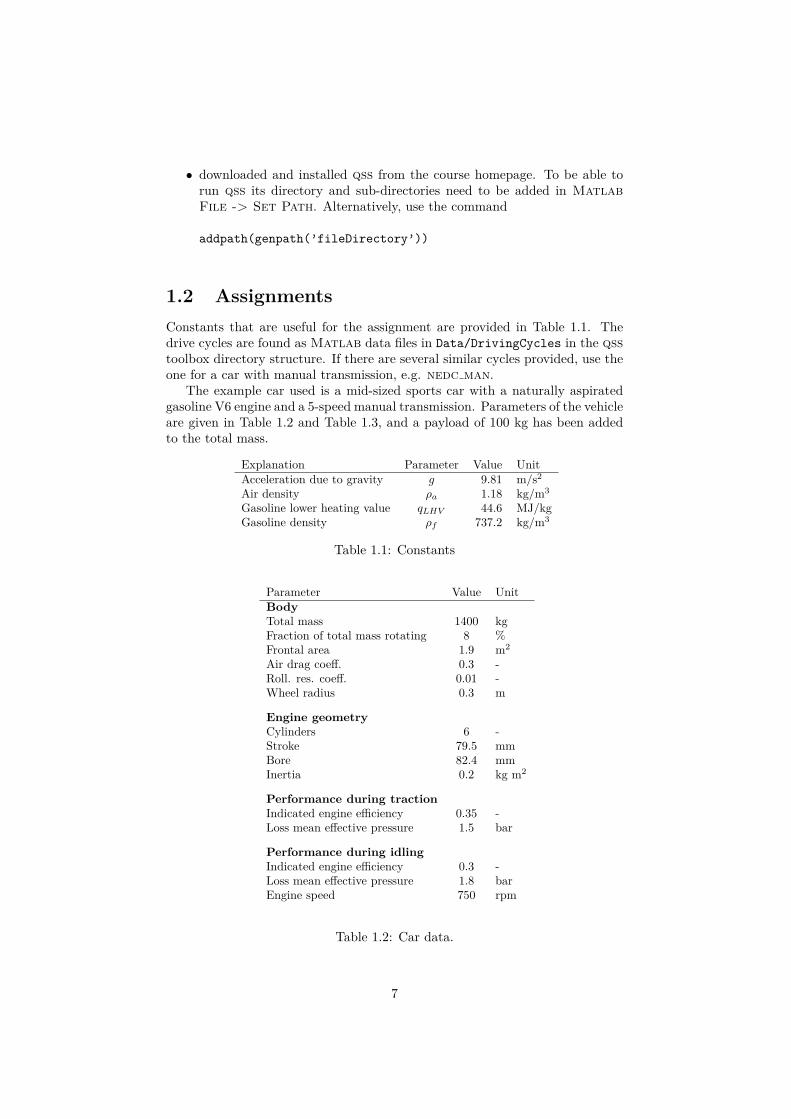
The example car used is a mid-sized sports car with a naturally aspiratedgasoline V6 engine and a 5-speed manual transmission. Parameters of the vehicleare given in Table 1.2 and Table 1.3, and a payload of 100 kg has been addedto the total mass.

Explanation Parameter Value UnitAcceleration due to gravity g 9.81 m/s2

Air density ρa 1.18 kg/m3

Gasoline lower heating value qLHV 44.6 MJ/kgGasoline density ρf 737.2 kg/m3

Table 1.1: Constants

Parameter Value UnitBodyTotal mass 1400 kgFraction of total mass rotating 8 %Frontal area 1.9 m2

Air drag coeff. 0.3 -Roll. res. coeff. 0.01 -Wheel radius 0.3 m

Engine geometryCylinders 6 -Stroke 79.5 mmBore 82.4 mmInertia 0.2 kg m2

Performance during tractionIndicated engine efficiency 0.35 -Loss mean effective pressure 1.5 bar

Performance during idlingIndicated engine efficiency 0.3 -Loss mean effective pressure 1.8 barEngine speed 750 rpm

Table 1.2: Car data.

7

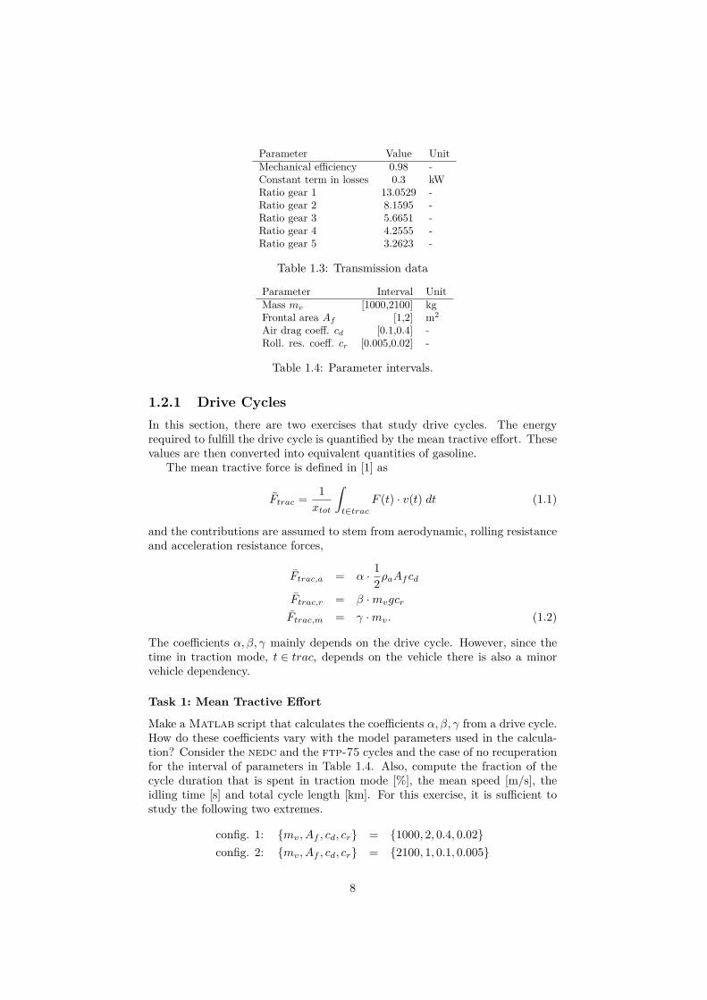
Parameter Value UnitMechanical efficiency 0.98 -Constant term in losses 0.3 kWRatio gear 1 13.0529 -Ratio gear 2 8.1595 -Ratio gear 3 5.6651 -Ratio gear 4 4.2555 -Ratio gear 5 3.2623 -

Table 1.3: Transmission data

Parameter Interval UnitMass mv [1000,2100] kgFrontal area Af [1,2] m2

Air drag coeff. cd [0.1,0.4] -Roll. res. coeff. cr [0.005,0.02] -

Table 1.4: Parameter intervals.

1.2.1 Drive CyclesIn this section, there are two exercises that study drive cycles. The energyrequired to fulfill the drive cycle is quantified by the mean tractive effort. Thesevalues are then converted into equivalent quantities of gasoline.

The mean tractive force is defined in [1] as

Ftrac = 1xtot

∫t∈trac

F (t) · v(t) dt (1.1)

and the contributions are assumed to stem from aerodynamic, rolling resistanceand acceleration resistance forces,

Ftrac,a = α · 12ρaAfcd

Ftrac,r = β ·mvgcr

Ftrac,m = γ ·mv. (1.2)

The coefficients α, β, γ mainly depends on the drive cycle. However, since thetime in traction mode, t ∈ trac, depends on the vehicle there is also a minorvehicle dependency.

Task 1: Mean Tractive Effort

Make a Matlab script that calculates the coefficients α, β, γ from a drive cycle.How do these coefficients vary with the model parameters used in the calcula-tion? Consider the nedc and the ftp-75 cycles and the case of no recuperationfor the interval of parameters in Table 1.4. Also, compute the fraction of thecycle duration that is spent in traction mode [%], the mean speed [m/s], theidling time [s] and total cycle length [km]. For this exercise, it is sufficient tostudy the following two extremes.

config. 1: mv, Af , cd, cr = 1000, 2, 0.4, 0.02config. 2: mv, Af , cd, cr = 2100, 1, 0.1, 0.005

8

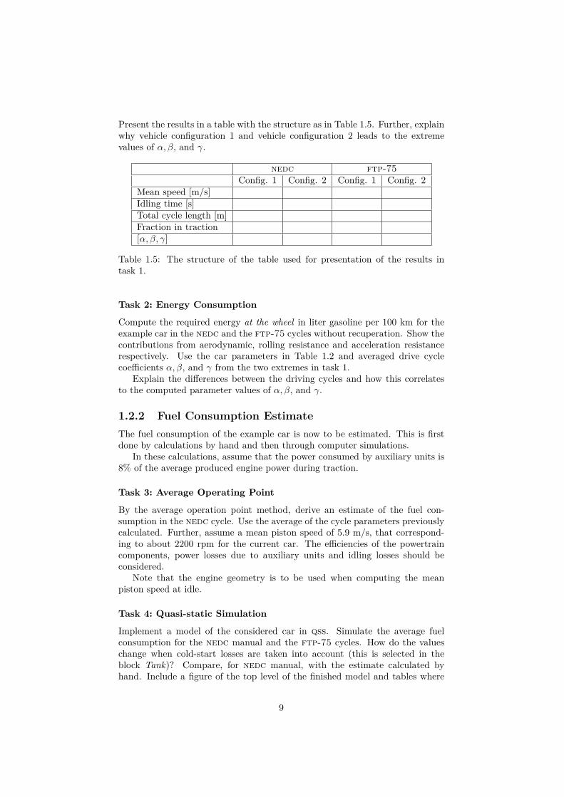
Present the results in a table with the structure as in Table 1.5. Further, explainwhy vehicle configuration 1 and vehicle configuration 2 leads to the extremevalues of α, β, and γ.

nedc ftp-75Config. 1 Config. 2 Config. 1 Config. 2

Mean speed [m/s]Idling time [s]Total cycle length [m]Fraction in traction[α, β, γ]

Table 1.5: The structure of the table used for presentation of the results intask 1.

Task 2: Energy Consumption

Compute the required energy at the wheel in liter gasoline per 100 km for theexample car in the nedc and the ftp-75 cycles without recuperation. Show thecontributions from aerodynamic, rolling resistance and acceleration resistancerespectively. Use the car parameters in Table 1.2 and averaged drive cyclecoefficients α, β, and γ from the two extremes in task 1.

Explain the differences between the driving cycles and how this correlatesto the computed parameter values of α, β, and γ.

1.2.2 Fuel Consumption EstimateThe fuel consumption of the example car is now to be estimated. This is firstdone by calculations by hand and then through computer simulations.

In these calculations, assume that the power consumed by auxiliary units is8% of the average produced engine power during traction.

Task 3: Average Operating Point

By the average operation point method, derive an estimate of the fuel con-sumption in the nedc cycle. Use the average of the cycle parameters previouslycalculated. Further, assume a mean piston speed of 5.9 m/s, that correspond-ing to about 2200 rpm for the current car. The efficiencies of the powertraincomponents, power losses due to auxiliary units and idling losses should beconsidered.

Note that the engine geometry is to be used when computing the meanpiston speed at idle.

Task 4: Quasi-static Simulation

Implement a model of the considered car in qss. Simulate the average fuelconsumption for the nedc manual and the ftp-75 cycles. How do the valueschange when cold-start losses are taken into account (this is selected in theblock Tank)? Compare, for nedc manual, with the estimate calculated byhand. Include a figure of the top level of the finished model and tables where

9

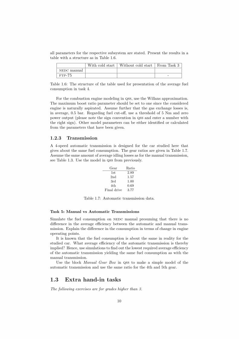
all parameters for the respective subsystem are stated. Present the results in atable with a structure as in Table 1.6.

With cold start Without cold start From Task 3nedc manualftp-75 -

Table 1.6: The structure of the table used for presentation of the average fuelconsumption in task 4.

For the combustion engine modeling in qss, use the Willans approximation.The maximum boost ratio parameter should be set to one since the consideredengine is naturally aspirated. Assume further that the gas exchange losses is,in average, 0.5 bar. Regarding fuel cut-off, use a threshold of 5 Nm and zeropower output (please note the sign convention in qss and enter a number withthe right sign). Other model parameters can be either identified or calculatedfrom the parameters that have been given.

1.2.3 TransmissionA 4-speed automatic transmission is designed for the car studied here thatgives about the same fuel consumption. The gear ratios are given in Table 1.7.Assume the same amount of average idling losses as for the manual transmission,see Table 1.3. Use the model in qss from previously.

Gear Ratio1st 2.892nd 1.573rd 1.004th 0.69

Final drive 3.77

Table 1.7: Automatic transmission data.

Task 5: Manual vs Automatic Transmissions

Simulate the fuel consumption on nedc manual presuming that there is nodifference in the average efficiency between the automatic and manual trans-mission. Explain the difference in the consumption in terms of change in engineoperating points.

It is known that the fuel consumption is about the same in reality for thestudied car. What average efficiency of the automatic transmission is therebyimplied? Hence, use simulations to find out the lowest required average efficiencyof the automatic transmission yielding the same fuel consumption as with themanual transmission.

Use the block Manual Gear Box in qss to make a simple model of theautomatic transmission and use the same ratio for the 4th and 5th gear.

1.3 Extra hand-in tasksThe following exercises are for grades higher than 3.

10

Extra task 1: Tolerances on velocity profile 2 p

The velocity profiles that are specified have tolerances, stating that you areallowed to deviate from the nominal profile with ±1 km/h. These toleranceshave an effect on the fuel consumption, but how large can they be?

Compute the required energy at the wheel in liter gasoline per 100 km for theexample car in the nedc and the ftp-75 cycles without recuperation, for thethree cases: nominal profile, maximum velocity profile, and minimum velocityprofile. State your assumptions and explain the results.

Extra task 2: Mild hybrid with stop-go functionality 2 p

Investigation of mild hybrid, with only stop-go functionality. How much fuelis saved if the engine is shut off during the idle periods in the cycle? Use theconventional vehicle in QSS described above to study this effect.

1.3.1 Extra task using forward modelingIn this task forward simulation is used, i.e. the model is based on dynamicequations. In order to perform the task, a simulation model can be downloadedfrom the course home page. There are three driving cycles available and youneed to load one of these before you start the simulation. These driving cyclesinclude more information than the driving cycles available in QSS.

Extra task 3: Compare quasi stationary and dynamic modeling 4 p

The objective of this task is to get an understanding of the differences be-tween quasi stationary simulation and forward simulation. You are supposedto parametrize the given model to represent the sports car. Assume that allcomponents except the chassis have zero mass. Note that for some componentsyou need to parametrize the controller as well.

Compare the simulated fuel consumption and simulation time using QSSand the dynamic model. Explain the differences, especially in simulation time.Present the values of the parameters used. It is only necessary to present thevalues of the parameters that differ from the values from Task 4 that was donein QSS, if any.

The component models used in the dynamic model are very similar to themodels in QSS. In cases where there are differences in the parametrization ofthe models, try to set values making the models as comparable as possible.

11

Hand-In 2

Dynamic ProgrammingOptimization of HybridVehicle Fuel Consumption

PurposeAcquire knowledge and experience concerning how to solve optimal controlproblems using Deterministic Dynamic Programming DDP. Acquire knowledgeabout the differences between parallel and series hybrid configurations and theirproperties.

Examination requirement• All tasks specified in Section 2.2.2 must be completed.

• Tasks specified in Section 2.3 are for grades higher than 3.

2.1 IntroductionFor environmental reasons as well as economical, minimization of fuel consump-tion is an urgent problem to solve. The hybrid vehicle with its possibility ofcharging and discharging battery gives us a mean to reduce fuel consumption.The challenge is to design a control that decides when to use the electrical motorand when to run the engine. If the driving mission is not known, this is a dif-ficult task. Depending on the driving cycle (speed, gearshifts, topography) thefuel consumption is reduced more or less when using a common hybrid vehicle.If the driving cycle is not known it is also important to have safety margins sothat the battery isn’t completely discharged.

However, if the driving cycle is known it is possible to find the global min-imum of fuel consumption, i.e. the best way possible to control the vehicle.One way of finding the global minimum is by using dynamic programming. Thedynamic programming for this assignment finds the minimum by dividing thedriving cycle in sections and gets the optimal control from each interior positionto the end of the driving cycle.

12

Prerequisites for the task

• Chapters 1-4 and Appendix III in the Vehicle Propulsion Systems book,[1]. Only parts of chapter 4 is needed to solve the task.

• Case study 2 in the Vehicle Propulsion Systems book, [1].

2.2 AssignmentsA hybrid vehicle has various possibilities of configurations. The parallel and theseries hybrid vehicle are two well known concepts. The parallel hybrid has amechanical link (via transmission) from the combustion engine to the wheels.In the series hybrid the combustion engine charges the battery and the electricalmotor is connected to the output shaft. This means that for the parallel hybridonly the state of charge is optimized, while the series hybrid has the possibilityof controlling both state of charge and the rotational speed of the engine.

The models for the parallel and the series hybrid, should be formulatedso that the cost for following an arc in the optimal control problem can becalculated.

2.2.1 Information and dataVehicle Parameters

Parameters for vehicle, driveline, engine, battery and electrical motor are givenin the following three tables: Table 2.1 gives the parameters that are commonfor both configurations, Table 1.3 gives the parameters for the transmission(neglect the constant losses in the gearbox) that are to be used in the parallelhybrid, and Table 2.2 gives the parameters specific for the series hybrid. In theseries hybrid, it is not possible to get Ne > 800rpm in the time step when theengine is started. In this time step the engine is not capable of delivering anytorque to the driveline.

Driving cycles

Many different driving cycles are used for simulation and certification purposes.The two driving cycles to be used here specifies speed [m/s], gear [-], acceleration[m/s2] and time [s]. The extra-urban driving cycle (EUDC MAN DDP.mat) startsby ramping up speed, which is continued by cruising on highway, and finallyspeed is ramped down. The city driving cycle (City MAN DDP.mat) representsaccelerations and stops that could occur in a city environment. The drivingcycles are available on the homepage, and are only slightly modified in the gearselection at almost stand still compared to the driving cycles included in QSS.

Cost function

The cost function is the function that is minimized by the dynamic program-ming. The objective of this assignment is to minimize the fuel consumption.This must be reflected in the cost function.

Also the states in the final time step could hold a cost. If there is no costrelated to the final time step, the final state will be the one that requires theleast fuel along the driving cycle, e.g. resulting in a low state of charge.

13

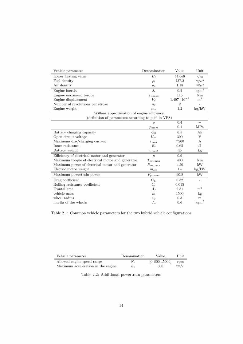
Vehicle parameter Denomination Value UnitLower heating value Hl 44.6e6 J/kg

Fuel density ρl 737.2 kg/m3

Air density ρa 1.18 kg/m3

Engine inertia Je 0.2 kgm2

Engine maximum torque Te,max 115 NmEngine displacement Vd 1.497 · 10−3 m3

Number of revolutions per stroke nr 2 -Engine weight me 1.2 kg/kW

Willans approximation of engine efficiency:(definition of parameters according to p.46 in VPS)

e 0.4 −pme,0 0.1 MPa

Battery charging capacity Q0 6.5 AhOpen circuit voltage Uoc 300 VMaximum dis-/charging current Imax ∓200 AInner resistance Ri 0.65 ΩBattery weight mbatt 45 kgEfficiency of electrical motor and generator η 0.9 -Maximum torque of electrical motor and generator Tem,max 400 NmMaximum power of electrical motor and generator Pem,max ∓50 kWElectric motor weight mem 1.5 kg/kWMaximum powertrain power Ppt,max 90.8 kWDrag coefficient CD 0.32 -Rolling resistance coefficient Cr 0.015 -Frontal area Af 2.31 m2

vehicle mass m 1500 kgwheel radius rw 0.3 minertia of the wheels Jw 0.6 kgm2

Table 2.1: Common vehicle parameters for the two hybrid vehicle configurations

Vehicle parameter Denomination Value UnitAllowed engine speed range Ne [0, 800...5000] rpmMaximum acceleration in the engine we 300 rad/s2

Table 2.2: Additional powertrain parameters

14

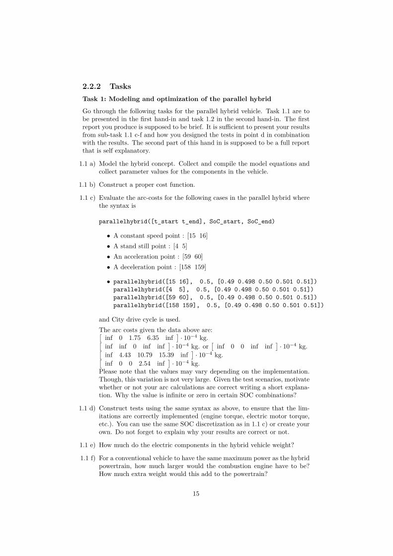
2.2.2 TasksTask 1: Modeling and optimization of the parallel hybrid

Go through the following tasks for the parallel hybrid vehicle. Task 1.1 are tobe presented in the first hand-in and task 1.2 in the second hand-in. The firstreport you produce is supposed to be brief. It is sufficient to present your resultsfrom sub-task 1.1 c-f and how you designed the tests in point d in combinationwith the results. The second part of this hand in is supposed to be a full reportthat is self explanatory.

1.1 a) Model the hybrid concept. Collect and compile the model equations andcollect parameter values for the components in the vehicle.

1.1 b) Construct a proper cost function.

1.1 c) Evaluate the arc-costs for the following cases in the parallel hybrid wherethe syntax is

parallelhybrid([t_start t_end], SoC_start, SoC_end)

• A constant speed point : [15 16]• A stand still point : [4 5]• An acceleration point : [59 60]• A deceleration point : [158 159]

• parallelhybrid([15 16], 0.5, [0.49 0.498 0.50 0.501 0.51])parallelhybrid([4 5], 0.5, [0.49 0.498 0.50 0.501 0.51])parallelhybrid([59 60], 0.5, [0.49 0.498 0.50 0.501 0.51])parallelhybrid([158 159], 0.5, [0.49 0.498 0.50 0.501 0.51])

and City drive cycle is used.The arc costs given the data above are:[

inf 0 1.75 6.35 inf]· 10−4 kg.[

inf inf 0 inf inf]· 10−4 kg. or

[inf 0 0 inf inf

]· 10−4 kg.[

inf 4.43 10.79 15.39 inf]· 10−4 kg.[

inf 0 0 2.54 inf]· 10−4 kg.

Please note that the values may vary depending on the implementation.Though, this variation is not very large. Given the test scenarios, motivatewhether or not your arc calculations are correct writing a short explana-tion. Why the value is infinite or zero in certain SOC combinations?

1.1 d) Construct tests using the same syntax as above, to ensure that the lim-itations are correctly implemented (engine torque, electric motor torque,etc.). You can use the same SOC discretization as in 1.1 c) or create yourown. Do not forget to explain why your results are correct or not.

1.1 e) How much do the electric components in the hybrid vehicle weight?

1.1 f) For a conventional vehicle to have the same maximum power as the hybridpowertrain, how much larger would the combustion engine have to be?How much extra weight would this add to the powertrain?

15

Hint: The maximum powertrain power has to be computed taking intoaccount the power curves of the electric motor and the combustion engineas well as the component losses. This calculation is already done and thevalue is provided in Table 2.1, (Ppt,max).

Next we are going to use deterministic dynamic programming (DDP) to findthe optimal control trajectories of the hybrid vehicle for a couple different cases.For all cases calculate the fuel consumption for the optimal solution in [l/100km],also measure the computational time of the DDP algorithm. Evaluate all taskson both City and EUDC cycles, and put your results in a table.

1.2 a) How do you make sure that the strategy is charge sustaining?Hint: Check how DDP works and how one can make sure that an unde-sired final step is not selected. This will require you to add a suitable finalcost to some of the states.

1.2 b) Run the optimization for a conventional vehicle with the same maximumpower as the hybrid powertrain.Hint: Use the masses and scaling factors computed in 1.1 e-f. A con-venient way of “removing” the battery is to construct a state vector sothat all combinations violate a component limitation. This prevents thealgorithm from changing the current value of the battery SOC.

1.2 c) Rerun the same optimization as in 1.2 b) but now use the downsized enginefrom the hybrid powertrain.

1.2 d) Run the optimization for the hybrid powertrain but restrict the algorithmas done in 1.2 b) so it cannot use the battery.

1.2 e) Now run the DDP-algorithm for the full hybrid, allowing battery use. Plotthe results including optimal SOC and cost profiles. Tabulate your finaloptimal costs.

Task 2: Modeling and optimization of the series hybrid

Go through the following tasks for the series hybrid vehicle. Task 2.1 are to bepresented in the first hand-in and task 2.2 in the second hand-in.

2.1 a) Model the hybrid concept. Collect and compile the model equations andcollect parameter values for the components in the vehicle.Note: The electric machine limits should only be implemented on thegenerator.

2.1 b) Construct a proper cost function.

2.1 c) Evaluate the arc-costs for the following cases in the series hybrid wherethe syntax is

serieshybrid([t_start t_end], SoC_start, SoC_end, N_start, N_end)

• A constant speed point : [15 16]• A stand still point : [4 5]• An acceleration point : [59 60]

16

• A deceleration point : [158 159]

• serieshybrid([15 16], 0.5, [49 49.8 50 50.2 51]e-2, 3e3, 3e3)serieshybrid([4 5], 0.5, [49 49.8 50 50.2 51]e-2, 3e3, 3e3)serieshybrid([59 60], 0.5, [49 49.8 50 50.2 51]e-2, 3e3, 3e3)serieshybrid([158 159], 0.5, [49 49.8 50 50.2 51]e-2, 3e3, 3e3)

• serieshybrid([15 16], 0.5, [0.5], 3e3, [0 2 3 5]e3)serieshybrid([4 5], 0.5, [0.5], 3e3, [0 2 3 5]e3)serieshybrid([59 60], 0.5, [0.5], 3e3, [0 2 3 5]e3)serieshybrid([158 159], 0.5, [0.5], 3e3, [0 2 3 5]e3)

• serieshybrid([15 16], 0.5, [0.499 0.5], 0, [0 8 20]e2)serieshybrid([4 5], 0.5, [0.499 0.5], 0, [0 8 20]e2)serieshybrid([59 60], 0.5, [0.499 0.5], 0, [0 8 20]e2)serieshybrid([158 159], 0.5, [0.499 0.5], 0, [0 8 20]e2)

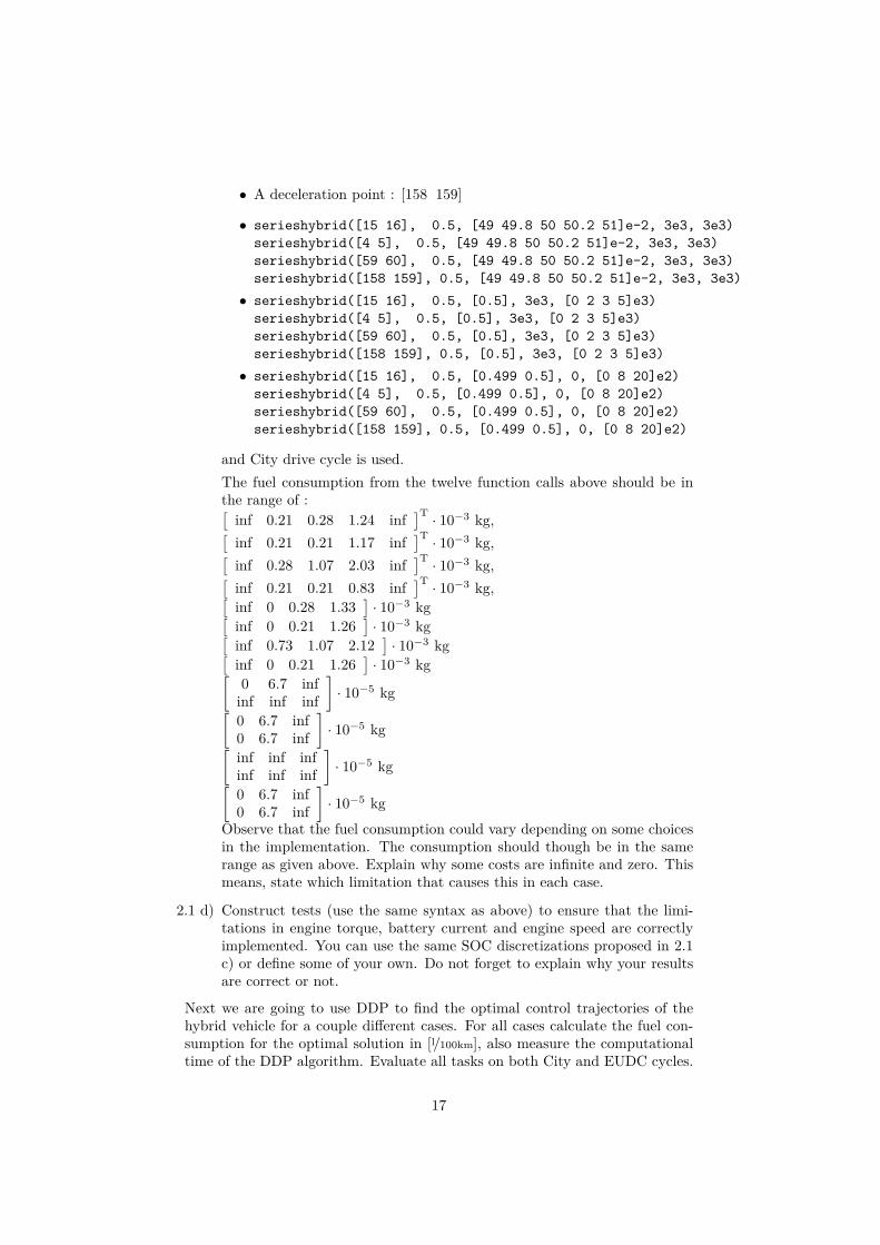
and City drive cycle is used.The fuel consumption from the twelve function calls above should be inthe range of :[

inf 0.21 0.28 1.24 inf]T · 10−3 kg,[

inf 0.21 0.21 1.17 inf]T · 10−3 kg,[

inf 0.28 1.07 2.03 inf]T · 10−3 kg,[

inf 0.21 0.21 0.83 inf]T · 10−3 kg,[

inf 0 0.28 1.33]· 10−3 kg[

inf 0 0.21 1.26]· 10−3 kg[

inf 0.73 1.07 2.12]· 10−3 kg[

inf 0 0.21 1.26]· 10−3 kg[

0 6.7 infinf inf inf

]· 10−5 kg[

0 6.7 inf0 6.7 inf

]· 10−5 kg[

inf inf infinf inf inf

]· 10−5 kg[

0 6.7 inf0 6.7 inf

]· 10−5 kg

Observe that the fuel consumption could vary depending on some choicesin the implementation. The consumption should though be in the samerange as given above. Explain why some costs are infinite and zero. Thismeans, state which limitation that causes this in each case.

2.1 d) Construct tests (use the same syntax as above) to ensure that the limi-tations in engine torque, battery current and engine speed are correctlyimplemented. You can use the same SOC discretizations proposed in 2.1c) or define some of your own. Do not forget to explain why your resultsare correct or not.

Next we are going to use DDP to find the optimal control trajectories of thehybrid vehicle for a couple different cases. For all cases calculate the fuel con-sumption for the optimal solution in [l/100km], also measure the computationaltime of the DDP algorithm. Evaluate all tasks on both City and EUDC cycles.

17

2.2 a) Make sure that the strategy is charge sustaining by adding a suitable costto some states in the final step.

2.2 b) Run the algorithm but restrict it so the battery remains unused.

2.2 c) Run the algorithm for the full hybrid. Plot the results including optimalSOC, engine speed and cost profiles. Tabulate your final optimal costs.

Task 3: Evaluation of results

• Which hybrid vehicle configuration requires the longest computationaltime to find optimal control by using dynamic programming? How bigis the difference? Is this consistent with the complexity of DDP algo-rithm? The time complexity can be described by the notation O(txmynz)where t, m, and n are the size of the time and state grids respectively.State the exponents x, y , and z for the parallel and series hybrids.

• How large consumption decrease comes from the downsizing of the engineand how much comes from the hybridization? Are there any drawbacksof just downsizing?

• Which hybrid configuration gets the lowest fuel consumption for the EUDCand City driving cycle respectively?Explain why. What can be said about the powertrain efficiencies?

2.3 Extra tasksIf you are interested in optimal control of hybrid vehicles, the following issuesmay be analyzed further

Extra task 1: More driving cycles 2 p

Analyze 4 additional driving cycles (eg. FTP-75, MVEG-95, Japan, . . . ) interms of fuel consumption and find optimal control for these. In each casewhere there is a configuration that is better, explain why that configuration isbest.

Extra task 2: Optimize the vehicle configuration 4 p

Optimize (or tune) the vehicle parameters (combination of engine and batterysizes etc) to give a better fuel consumption than the ones suggested above. Tryto find an optimum and provide an explanation for why these new parameterswere chosen.

Extra task 3: Gear ratios in the parallel hybrid 2 p

The gear ratios used in the mandatory task represent the sports car that alsois used in Hand in 1. Investigate how a modified gearbox with gear ratiosaccording to Table 2.3 will affect the fuel consumption. Explain the resultsand calculate how many revolutions per minute the engine will run using thedifferent gearboxes. Are there any drawbacks using the gearbox with lower gear

18

ratios? Which gearbox do you think most drivers would prefer? Note that thegear ratios in this task includes the gear ratio in the final gear.

Gear Gear ratio1 9.972 5.863 3.844 2.685 2.14

Table 2.3: Gear ratios in the modified gearbox.

Extra task 4: Heavy truck problem 12 p

Now we will study the possibilities that arise if the vehicle is a heavy truckand the driving cycle contains information about topography. For heavy trucksseemingly small slopes pose challenges for maintaining the vehicle speed. Thisis a problem that actually can be turned to an advantage for saving fuel. Byknowing the topography and considering the kinetic and potential energies asenergy storage.

For heavy trucks in long haul operation a typical scenario would be to gofrom A to B in a specified time, i.e. essentially the average speed is specified.Then the truck is allowed to deviate from this average speed and the goal is tominimize the fuel consumption. To solve this problem it is necessary to use twostates, one for the vehicle speed and one for the traveled distance.

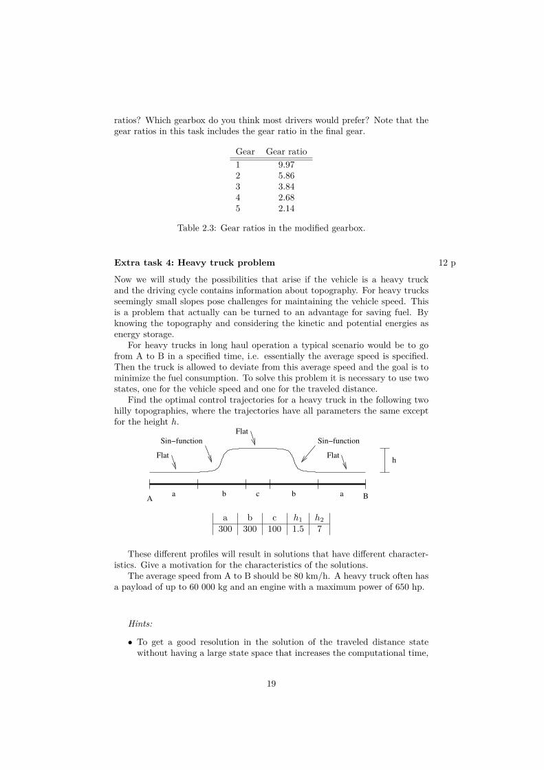
Find the optimal control trajectories for a heavy truck in the following twohilly topographies, where the trajectories have all parameters the same exceptfor the height h.

Sin−function

Flat

Flat

Flat

A Ba b c ab

h

Sin−function

a b c h1 h2300 300 100 1.5 7

These different profiles will result in solutions that have different character-istics. Give a motivation for the characteristics of the solutions.

The average speed from A to B should be 80 km/h. A heavy truck often hasa payload of up to 60 000 kg and an engine with a maximum power of 650 hp.

Hints:

• To get a good resolution in the solution of the traveled distance statewithout having a large state space that increases the computational time,

19

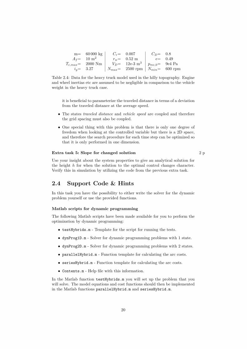
m= 60 000 kg Cr= 0.007 CD= 0.8Af = 10 m2 rw= 0.52 m e= 0.49

Te,max= 2000 Nm VD= 12e-3 m3 pme,0= 9e4 Paig= 3.27 Nmax= 2500 rpm Nmin= 600 rpm

Table 2.4: Data for the heavy truck model used in the hilly topography. Engineand wheel inertias etc are assumed to be negligible in comparison to the vehicleweight in the heavy truck case.

it is beneficial to parameterize the traveled distance in terms of a deviationfrom the traveled distance at the average speed.

• The states traveled distance and vehicle speed are coupled and thereforethe grid spacing must also be coupled.

• One special thing with this problem is that there is only one degree offreedom when looking at the controlled variable but there is a 2D space,and therefore the search procedure for each time step can be optimized sothat it is only performed in one dimension.

Extra task 5: Slope for changed solution 2 p

Use your insight about the system properties to give an analytical solution forthe height h for when the solution to the optimal control changes character.Verify this in simulation by utilizing the code from the previous extra task.

2.4 Support Code & HintsIn this task you have the possibility to either write the solver for the dynamicproblem yourself or use the provided functions.

Matlab scripts for dynamic programming

The following Matlab scripts have been made available for you to perform theoptimization by dynamic programming:

• testHybrids.m - Template for the script for running the tests.

• dynProg1D.m - Solver for dynamic programming problems with 1 state.

• dynProg2D.m - Solver for dynamic programming problems with 2 states.

• parallelHybrid.m - Function template for calculating the arc costs.

• seriesHybrid.m - Function template for calculating the arc costs.

• Contents.m - Help file with this information.

In the Matlab function testHybrids.m you will set up the problem that youwill solve. The model equations and cost functions should then be implementedin the Matlab functions parallelHybrid.m and seriesHybrid.m.

20

2.4.1 Hints• To save computational time it is a good idea to use the matrix formulation,

as is indicated in the Vehicle Propulsion Systems book [1].

• To save time, use a truncated or shorter profile time when implementingand debugging your code for the concepts.

21

Hand-In 3

Real-time Optimal Controlof Hybrid ElectricPowertrains

PurposeAcquire knowledge and experience about solving and implementing a real timeenergy management for a hybrid electric vehicle.

Examination requirement• All tasks specified in Section 3.2.2 must be completed.

• Tasks specified in Section 3.2.3 are for grades higher than 3.

3.1 IntroductionIn the previous task the optimal control solution to the energy managementproblem for hybrid electric vehicles was studied using dynamic programming.Dynamic programming is a powerful tool to study optimal control as well asto investigate the potential of different configurations. However, its computa-tional burden, as well as requirement for perfect look-ahead make it difficult toimplement in real-time energy management.

A common strategy in academia to solve the energy management problemin real time is equivalent consumption minimization strategy (ECMS). Insteadof minimizing

∫ T

0 mfdt which requires the entire driving mission to be knownthe problem is transformed to instead minimize a sum of power from fuel andbattery at each timestep. However these powers are not directly comparable soan equivalence factor is needed. The resulting expression to be minimized is ofhamiltonian form and can be written:

H = Pf + λPech

u∗ = arg minH(3.1)

22

where Pf is the power from fuel, Pech the power in the battery, λ an equiv-alence factor and u∗ the optimal control. This problem can be solved at eachtimestep, iff λ is known.

ECMS and Pontryagins maximum principle(PMP) are closely related. Fromthe PMPs necessary conditions for optimality we have:

∂H

∂x= −λ∗ (3.2)

where x are the states. This means that along the optimal trajectory, theoptimal time evolution of the equivalence factor λ has to be equal to the partialderivative of the hamiltonian with respect to the state.

Prerequisites for the task

• Chapter 7 and Case Study 7 in the Vehicle Propulsion Systems book, [1].

3.2 AssignmentsThe assignment is to be solved by using the QSS program package that can bedownloaded from the course homepage. A basic vehicle model called HEV_ECMS.mdlis provided on the course-page as well as two scripts init_HEV_ECMS.m andparallelhybrid_ECMS.m that should be completed in the task. You shoulddownload this material before continuing with the assignment. Remember thatyou always can study the already implemented QSS examples and the QSSlibrary if you are new so Simulink.

3.2.1 Information and dataVehicle Configuration

The considered configuration is the parallel hybrid studied previously. Theparameters of the provided model are not exactly the same so you will have tostudy the models to fill in the appropriate values.

3.2.2 Tasks1. Construct the Hamiltonian on paper, write down expressions for Pf andPech.

2. Using your Hamiltonian and (3.2) what is the optimal time evolution ofour equivalence factor, i.e. what is λ∗? Justify your response analytically.

3. Using the parallelhybrid.m from the dynamic programming excercise asbase, complete parallelhybrid_ECMS.m, i.e. given [ωice, ωice, Treq, λ]your script should return the optimal [Tice, Tem]Hint: Solve the optimization numerically.

4. Complete the models for the electric motor and combustion engine inHEV_ECMS.mdl, parametrize the gear box and vehicle model so it corre-sponds as close as possible to your parallelhybrid.m implementation.What is the function of init_HEV_ECMS.m? Also implement checks to see

23

that your controller does not violate any limits.Hint: Study the battery and Torque following-subsystems. Remember toinclude the inertia of the wheels in the rotating mass field of the QSS Ve-hicle block (Note that the block requires a % value, look under the blockmask to see how the model uses the rotating mass percentage and thushow you should compute its value). Include the engine inertia effects inthe engine block and not in the vehicle rotating mass, as you did in yourparallelhybrid.m implementation.

5. Find the optimal solution to the EUDC manual and City manual cyclesusing ECMS. What is the optimal λ(t) for the different driving cycles?Note: Due to discretization it can be hard to get SOC(T ) = SOC(1), buttry to get as close as possible while ensuring SOC(T ) ≥ SOC(1)

6. Compare the received solutions to the solutions from dynamic program-ming. Are there any differences? Computational time?

7. Use the driving cycles NEDC and FTP75. First find the optimal λ(t).Secondly, do a sensitivity analysis on λ(t), what happens if your openloop control is not perfect?

8. Given that the problem is unconstrained, the problem in (3.1) can besolved analytically. Solve the problem and find an expression for thecontrols. You need to analytically ensure that your derived expressionminimizes (and not maximizes) the Hamiltonian. When are the derivedcontrols applicable? When not?

3.2.3 Extra TaskIf you are interested in real time optimal control of hybrid vehicles, the followingissues may be analyzed further

Extra task 1: Implementing analytical solution 3 p

Implement the analytical solution to the ECMS problem. Compare the optimalλ to the previous implemented version, are there any differences?

24

Hand-In 4

Short Term Storage andSupervisory Control

This hand-in is not mandatory, but is an extra task that gives up to 12 points.

PurposeThis assignment deals with short term storage systems. The task is to applyeverything you have learned during the course to modify an existing vehicle byadding one or more short term storage systems. The goal is to minimize the fuelconsumption for the new vehicle using a smart control strategy and by choosinggear ratios and sizes of the add-ons in an optimal way.

Examination requirement• Three different concepts can be modeled, implemented, and analyzed.

• The demands on the contents of the final report stated in Section 4.1 mustbe fulfilled.

• Completing the supercap concept gives up to 8 points.

• Completing the flywheel concept gives up to 10 points.

• Completing the hydraulic concept gives up to 12 points.

• If you decide to do more than one concept 6 points will be deductedfrom the second and third concept.(This means doing only the flywheelconcept gives 10 points, doing both supercap and flywheel concepts gives12 points.)

4.1 Assignment specificationThe assignment is to be solved by using the QSS program package that can bedownloaded from the course homepage. A basic vehicle model called OrdinaryVehicle.mdl

25

is provided on the course-page as well as a script to make efficiency plots forenergy converters (mkPlots.m). You should download this material before con-tinuing with the assignment. Remember that you always can study the alreadyimplemented QSS examples and the QSS library.

Chapter 5 in the Vehicle Propulsion System book [1] covers short term stor-age systems, while Chapter 4 covers Hybrid-Electric propulsion systems.

The final report should at least contain the following

• The performance and engine efficiency plot of the conventional vehicleaccording to Section 4.1.1.

• Description and discussion of the final design and the design choices, aswell as the model equations and model parameters.

• Description and discussion of the QSS implementation. You are free to useother available QSS model blocks than the ones used in the basic vehiclemodel as long as the models conforms to he specifications in Section 4.2.

• Description and discussion of your chosen control strategy.

• Efficiency plots showing in what operating points your components areoperating. This is only necessary for components with a non constantefficiency and/or with torque/speed limits.

The report should be self explanatory and should not assume prior knowledgeto any of the used short term storage systems or components. All assumptionsshould be discussed and the control strategy should be well described, discussedand motivated.

You should also make believable that your fuel consumption is accurate.That is, you should explain where your design saves the most fuel and how thisaffects the total fuel consumption.

Available model components and assumptions are listed in Section 4.2 below.

4.1.1 Evaluation of vehicle demandsThe first assignment is to evaluate the provided vehicles performance and thedrive cycles energy demand for the specific vehicle. Therefore answer the fol-lowing questions:

• What is the maximum acceleration of the vehicle? This property can e.g.be given in the time to accelerate form 0 km/h to 100 km/h.

• What is the maximum speed of the vehicle?

• In what operating points does the engine operate when a driving cycle isused?

Approximate values for the first two questions are sufficient, and Chapter 2 in[1] is recommended. As a help for you to plot the operating points of the engine,there is a plot command mkPlots.m available for you to download.

26

4.1.2 Design of new vehicleChoose a short term storage concept. You may for example choose one ofthe concepts from Figure 5.2 in [1]. However, you are free to connect anycomponents you wish as long as it’s physically feasible and provided that youadd the components masses to the vehicle mass.

Write down the equations for all the components of the modeled vehicle.Then chose component sizes, gear ratios and other quantities. Plot finally theefficiency maps as well as limiting factors where applicable and ensure that

1. All operating points will be within the limits for the used components.

2. The components will be operating close to the maximum efficiency whenworking together.

3. The short term storage system[s] are large enough.

If you are uncertain of how to implement your concept in QSS you may lookat the QSS built-in examples, especially qss example shv. Also remember thatthe Matlab/Simulink blocks Scope and To Workspace are your friends.

4.1.3 Design of control strategyA control strategy is an algorithm that decides where to take the energy that isneeded by the vehicle-drivecycle pair and how to utilize the short term storage.The control strategy should be designed so that the vehicle can perform thewhole drive cycle without running into torque/speed limits and so that thecombustion engine as well as the other components are operated in an efficientway.

4.1.4 Evaluation of new Vehicle and control strategyShow how your vehicle/control-strategy works together. Use efficiency plots thatshow what operating points your components are operating in. Have you chosenthe right gear ratios and sizes for your vehicle? Make a parameter study to seehow sensitive your fuel consumption is to the model parameters for your shortterm storage components as well as your control strategy. Here it is importantto not favor parameter choices that drains the short term storage system.

Also make believable that your fuel consumption is accurate. That is, ex-plain where your design saves the most fuel and how this affects the total fuelconsumption.

4.2 Available models and assumptionsFirst is a list of the available components you are allowed to add as well ascommon model assumptions and then a detailed walk through of some of thecomponents.

• Flywheels

• Hydraulic Accumulators

• Supercapacitors

27

as well as the following glue components

• Gearboxes

• Electric motors

• Electric generators

• Continously variable transmissions

• Hydraulic pumps/motors

• Torque couplers and planetary gear sets

• Power electronics

All short term storage devices should have the same, or higher, charge statusafter the driving cycle as before, otherwise this has to be accounted for in arealistic way.

4.2.1 Short term storage systemsThe equations for the short term storage systems are specified in the courseliterature unless available here as a reference. Parameters are to be chosenwithin reasonable limitations. Investigate how different parameters (e.g. thespeed of the flywheel, charge of the hydraulic accumulator or supercapacitor,and power) affect the efficiency of the component(s) used. This can e.g. bedone using the Peukert or Ragone tests for the supercapacitor and hydraulicaccumulator.

Flywheel

Assume that you are able to make flywheels using a material with ρ = 8000[kg/m3] and are able to choose b, d and q freely within reasonable limits. Alsoassume that manufacturing limitations gives you the flywheel parameters inTable 4.1. Assume that the total weight of the flywheel and bearings is 5%more than the flywheel mass.

Parameter Description Valueρ Flywheel density 8000 [kg/m3]ρa Ambient air density 1.29 [kg/m3]ηa Dynamic air viscosity 1.72 ·10−5 [Pa s]b Width By choiced Diameter By choiceq Inner/Outer diameter ratio q ∈ [0, 1]dw/d Shaft/Wheel ratio 0.08 [-]µ Friction coefficient 1.5 · 10−3 [-]k Unbalance factor 4 [-]ωmax Maximum speed 30 000 [rpm]mtot Total mass 1.05 ·mf

Table 4.1: Flywheel parameters from the flywheel manufacturer.

28

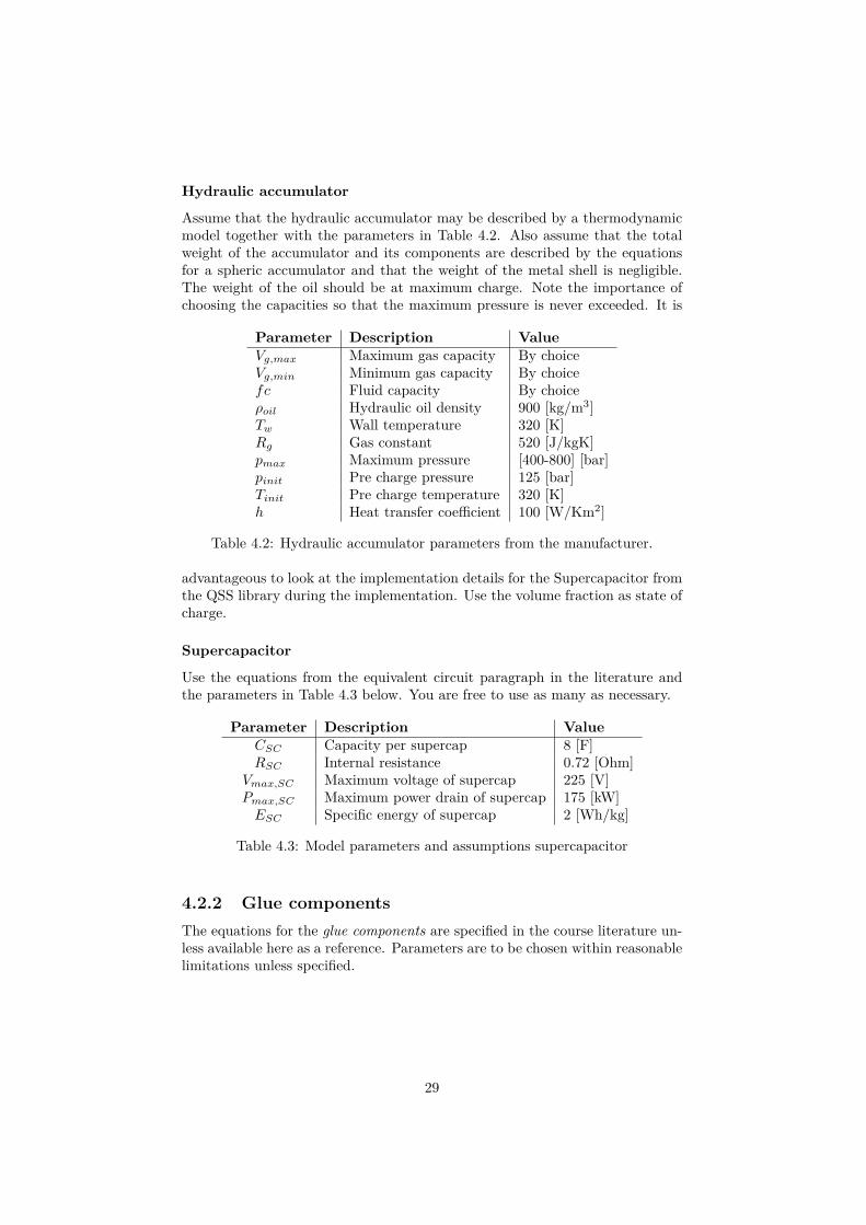
Hydraulic accumulator

Assume that the hydraulic accumulator may be described by a thermodynamicmodel together with the parameters in Table 4.2. Also assume that the totalweight of the accumulator and its components are described by the equationsfor a spheric accumulator and that the weight of the metal shell is negligible.The weight of the oil should be at maximum charge. Note the importance ofchoosing the capacities so that the maximum pressure is never exceeded. It is

Parameter Description ValueVg,max Maximum gas capacity By choiceVg,min Minimum gas capacity By choicefc Fluid capacity By choiceρoil Hydraulic oil density 900 [kg/m3]Tw Wall temperature 320 [K]Rg Gas constant 520 [J/kgK]pmax Maximum pressure [400-800] [bar]pinit Pre charge pressure 125 [bar]Tinit Pre charge temperature 320 [K]h Heat transfer coefficient 100 [W/Km2]

Table 4.2: Hydraulic accumulator parameters from the manufacturer.

advantageous to look at the implementation details for the Supercapacitor fromthe QSS library during the implementation. Use the volume fraction as state ofcharge.

Supercapacitor

Use the equations from the equivalent circuit paragraph in the literature andthe parameters in Table 4.3 below. You are free to use as many as necessary.

Parameter Description ValueCSC Capacity per supercap 8 [F]RSC Internal resistance 0.72 [Ohm]

Vmax,SC Maximum voltage of supercap 225 [V]Pmax,SC Maximum power drain of supercap 175 [kW]ESC Specific energy of supercap 2 [Wh/kg]

Table 4.3: Model parameters and assumptions supercapacitor

4.2.2 Glue componentsThe equations for the glue components are specified in the course literature un-less available here as a reference. Parameters are to be chosen within reasonablelimitations unless specified.

29

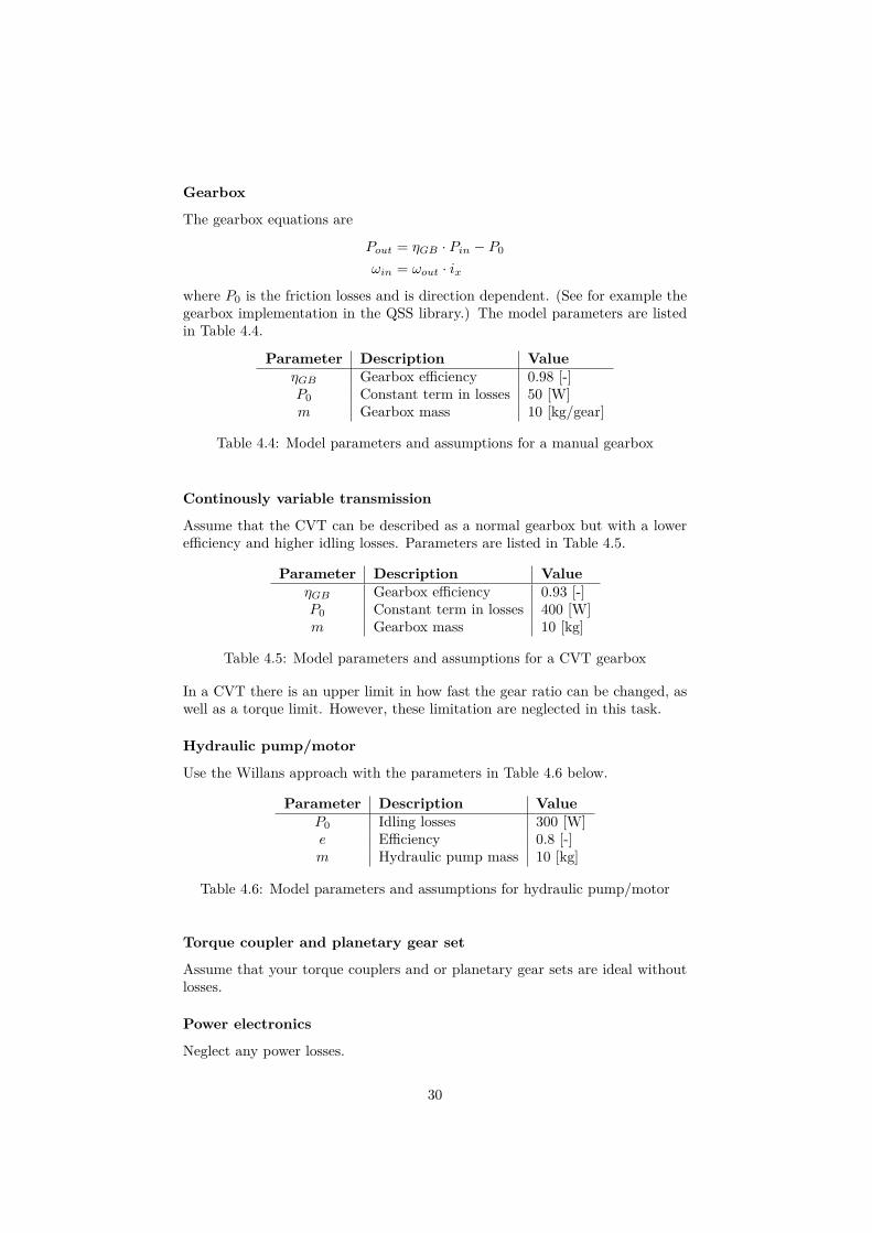
Gearbox

The gearbox equations are

Pout = ηGB · Pin − P0

ωin = ωout · ix

where P0 is the friction losses and is direction dependent. (See for example thegearbox implementation in the QSS library.) The model parameters are listedin Table 4.4.

Parameter Description ValueηGB Gearbox efficiency 0.98 [-]P0 Constant term in losses 50 [W]m Gearbox mass 10 [kg/gear]

Table 4.4: Model parameters and assumptions for a manual gearbox

Continously variable transmission

Assume that the CVT can be described as a normal gearbox but with a lowerefficiency and higher idling losses. Parameters are listed in Table 4.5.

Parameter Description ValueηGB Gearbox efficiency 0.93 [-]P0 Constant term in losses 400 [W]m Gearbox mass 10 [kg]

Table 4.5: Model parameters and assumptions for a CVT gearbox

In a CVT there is an upper limit in how fast the gear ratio can be changed, aswell as a torque limit. However, these limitation are neglected in this task.

Hydraulic pump/motor

Use the Willans approach with the parameters in Table 4.6 below.

Parameter Description ValueP0 Idling losses 300 [W]e Efficiency 0.8 [-]m Hydraulic pump mass 10 [kg]

Table 4.6: Model parameters and assumptions for hydraulic pump/motor

Torque coupler and planetary gear set

Assume that your torque couplers and or planetary gear sets are ideal withoutlosses.

Power electronics

Neglect any power losses.

30

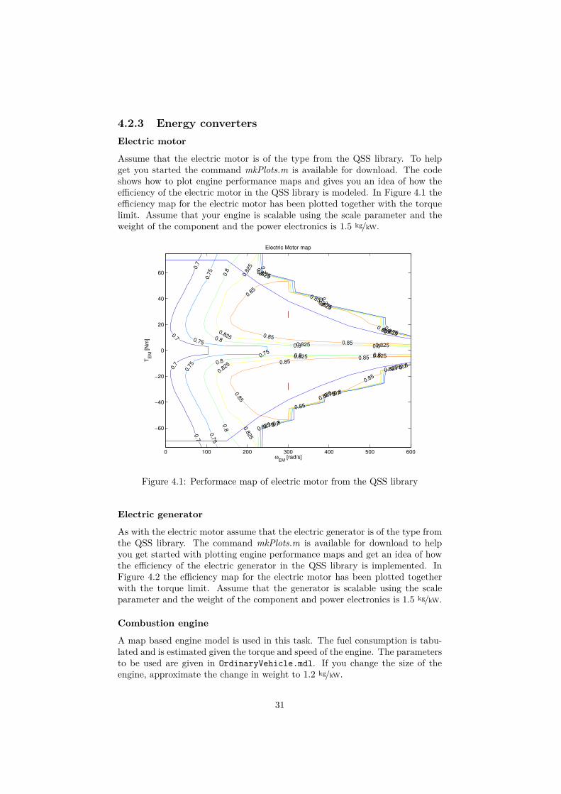
4.2.3 Energy convertersElectric motor

Assume that the electric motor is of the type from the QSS library. To helpget you started the command mkPlots.m is available for download. The codeshows how to plot engine performance maps and gives you an idea of how theefficiency of the electric motor in the QSS library is modeled. In Figure 4.1 theefficiency map for the electric motor has been plotted together with the torquelimit. Assume that your engine is scalable using the scale parameter and theweight of the component and the power electronics is 1.5 kg/kW.

0.7

0.7

0.7

0.7

0.7

0.7

0.7

0.7

0.7

0.7

0.7

5

0.75

0.75

0.75

0.7

5

0.75

0.75

0.75

0.75

0.75

0.75

0.8

0.80.8 0.8

0.8

0.80.8 0.8

0.8

0.8

0.8

0.8

0.8

0.8

0.82

5

0.825

0.825 0.825

0.8

25

0.825

0.825 0.825

0.825

0.825

0.825

0.825

0.825

0.825

0.85

0.850.8

5

0.850.85

0.850.85

0.85

0.85

0.85

ωEM

[rad/s]

TE

M [N

m]

Electric Motor map

0 100 200 300 400 500 600

−60

−40

−20

0

20

40

60

Figure 4.1: Performace map of electric motor from the QSS library

Electric generator

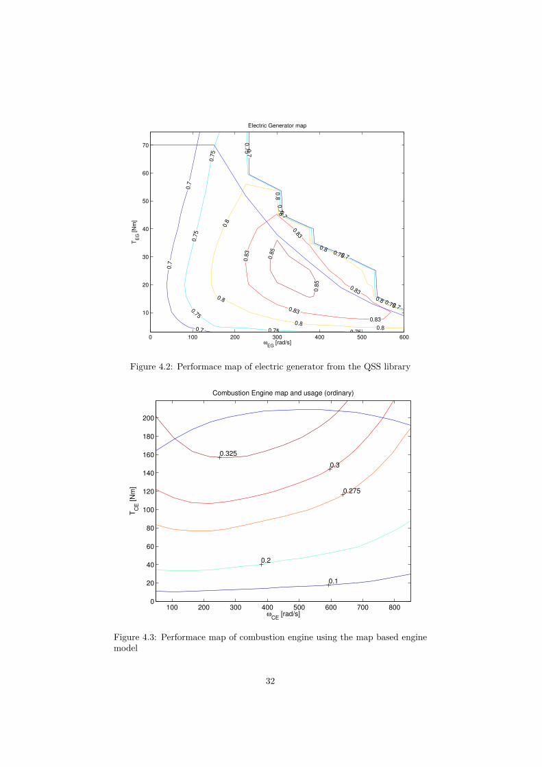
As with the electric motor assume that the electric generator is of the type fromthe QSS library. The command mkPlots.m is available for download to helpyou get started with plotting engine performance maps and get an idea of howthe efficiency of the electric generator in the QSS library is implemented. InFigure 4.2 the efficiency map for the electric motor has been plotted togetherwith the torque limit. Assume that the generator is scalable using the scaleparameter and the weight of the component and power electronics is 1.5 kg/kW.

Combustion engine

A map based engine model is used in this task. The fuel consumption is tabu-lated and is estimated given the torque and speed of the engine. The parametersto be used are given in OrdinaryVehicle.mdl. If you change the size of theengine, approximate the change in weight to 1.2 kg/kW.

31

0.7

0.7

0.7

0.7

0.70.7

0.7

0.7

5

0.7

5

0.75

0.75 0.75

0.7

5

0.7

5

0.75

0.75

0.8

0.8

0.8

0.8

0.8

0.80.8

0.83

0.83

0.8

30.83

0.830.8

5

0.8

5

ωEG

[rad/s]

TE

G [N

m]

Electric Generator map

0 100 200 300 400 500 600

10

20

30

40

50

60

70

Figure 4.2: Performace map of electric generator from the QSS library

Combustion Engine map and usage (ordinary)

ωCE

[rad/s]

TC

E [N

m]

0.1

0.2

0.275

0.3

0.325

100 200 300 400 500 600 700 8000

20

40

60

80

100

120

140

160

180

200

Figure 4.3: Performace map of combustion engine using the map based enginemodel

32

Hand-In 5

Fuel Cell and SupervisoryControl

This hand-in is not mandatory, but is an extra task that gives up to 14 points.

PurposeIn this hand-in you are supposed to implement a fuel cell vehicle in Simulinkusing forward modeling. The purpose is twofold:

• get knowledge about how a fuel cell works and evaluate efficiencies andfuel consumption of a fuel cell vehicle.

• get familiar with forward modeling.

Examination requirement• The vehicle should fulfill the specifications given in section 5.1.1.

• Calculate the fuel consumption using hydrogen as fuel. The fuel con-sumption is preferably presented in equivalent gasoline consumption per100 km. Use NEDC.

• Calculate the fuel consumption if methanol is used as fuel instead of hy-drogen, (use information in section 5.2.1). Compare this result to a con-ventional vehicle equipped with an SI engine. Make the comparison interms of both the energy consumption and CO2 emissions.Hint: To calculate the CO2 emissions, assume stoichiometric mixture. Usethe results from hand-in 1 for the conventional vehicle.

• Calculate the average efficiency of the fuel cell, electric machine and thebuffer.

33

5.1 Assignment specificationThe assignment is to be solved using Simulink and a given model skeleton thatcan be downloaded from the course homepage. Chapter 6 in the Vehicle Propul-sion System book [1] covers fuel cells. It might also be helpful to study the modelimplemented in QSS.

The final report must at least contain the following:

• Description and discussion of the design, including values of importantparameters of your model.

• Description and discussion of your chosen control strategy.

• Plots showing the efficiency and operating points of your components.

The report should be self explanatory and all the components included in themodel must be documented. All assumptions should be discussed and the con-trol strategy should be well described, discussed, and motivated.

You should also evaluate and provide support for the credibility of yourfuel consumption estimate. Furthermore, you should explain where your designsaves the most fuel and how this affects the total fuel consumption.

5.1.1 Vehicle demandsTo be able to compare the conventional vehicle to the vehicle developed in thisassignment, the vehicle should manage to

• accelerate from stand still to 100 km/h in 15 s,

• have a sustained top speed of at least 160 km/h, and

• have high overall efficiency on the NEDC.

Vehicle and component parameters, such as the specific weights, are given insection 5.3.

5.1.2 Design of new vehicleWrite down the equations for all the components of the modeled vehicle. Thenchoose component sizes and other quantities. Make sure the vehicle fulfills therequirements in section 5.1.1. Finally plot the efficiencies (for the fuel cell, thiscould be efficiency against power), as well as limiting factors where applicable.Ensure that

1. all operating points will be within the limits for the used components,

2. the components will be operating close to the maximum efficiency whenworking together, and

3. the short term storage system[s] are large enough.

5.1.3 Design of control strategyA control strategy with the same demands as described in section 4.1.3 is to beimplemented.

34

5.2 Available models and assumptionsThere are some models included in the skeleton that you can use. You are ofcourse free to develop and add new models of the components. Skeletons forthe controller and fuel cell are included in the given skeleton, which you areto add functionality to. Observe that the vehicle model is sensitive for namingof the signals, since buses are used. The parameters of the components are tobe chosen in order to fulfill the requirements in section 5.1.1. You are free tochoose any configuration of the vehicle you want to, as long as it is physicallypossible to construct. There is one concept of a fuel cell vehicle chosen in thegiven skeleton that you can use.

5.2.1 FuelYou are supposed to implement a model of a vehicle that uses hydrogen as fuel,i.e. there is no reformer in the vehicle. This should result in a relatively highoverall efficiency of the vehicle. The disadvantages associated with this technol-ogy are for example that hydrogen storage is problematic, new infrastructure isneeded, and that transportation of hydrogen is costly.

An alternative is to use methanol as fuel and use a reformer on-board thatproduces hydrogen. Assume that the reformer has a mean efficiency of 55 %,and that the lower heating value of methanol is 19.8 MJ/kg.

5.3 Vehicle DataIn this section some data to be used in the modeling of the fuel cell vehicle isgiven. For the data not presented in this section, use the parameters for thesports car in Hand-in 1.

5.3.1 Fuel cellThe fuel cell has slower dynamics than for example an ICE. Therefore it is notadequate to assume that the requested power from the fuel cell is deliveredinstantaneously, if there is a change in the power demanded. In this task thisis modeled using a first order low pass filter with a time constant of 5 seconds.Data needed for one cell in the stack is given in Table 5.1.

5.3.2 Super capacitorA buffer consists of several cells connected in series and in some cases paral-lel. You are free to design the buffer as long as you use realistic parameters.The following data for a cell in the super capacitor is just an example of themagnitude of the parameters. The capacitance is 3 F, voltage 2.5 V and innerresistance 2 mΩ. The inner resistance is a relative large value. This is to modelthe losses due to leakage currents in the capacitor since that is not a part of thegiven model. If you wish to use other parameters http://www.maxwell.com isa good place to start looking.

35

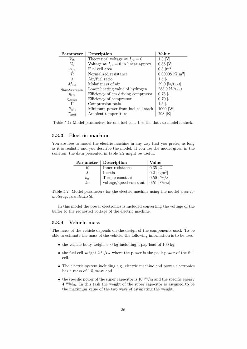
Parameter Description ValueVth Theoretical voltage at Ifc = 0 1.3 [V]V0 Voltage at Ifc = 0 in linear approx. 0.88 [V]Afc Fuel cell area 0.3 [m2]R Normalized resistance 0.00008 [Ω m2]λ Air/fuel ratio 1.5 [-]

Mair Molar mass of air 29.0 [kg/kmol]qlhv,hydrogen Lower heating value of hydrogen 285.9 MJ/kmol

ηem Efficiency of em driving compressor 0.75 [-]ηcomp Efficiency of compressor 0.70 [-]

Π Compression ratio 1.3 [-]Pidle Minimum power from fuel cell stack 1000 [W]Tamb Ambient temperature 298 [K]

Table 5.1: Model parameters for one fuel cell. Use the data to model a stack.

5.3.3 Electric machineYou are free to model the electric machine in any way that you prefer, as longas it is realistic and you describe the model. If you use the model given in theskeleton, the data presented in table 5.2 might be useful.

Parameter Description ValueR Inner resistance 0.35 [Ω]J Inertia 0.2 [kgm2]ka Torque constant 0.50 [Nm/A]ki voltage/speed constant 0.51 [Vs/rad]

Table 5.2: Model parameters for the electric machine using the model electric-motor quasistatic2 std.

In this model the power electronics is included converting the voltage of thebuffer to the requested voltage of the electric machine.

5.3.4 Vehicle massThe mass of the vehicle depends on the design of the components used. To beable to estimate the mass of the vehicle, the following information is to be used:

• the vehicle body weight 900 kg including a pay-load of 100 kg,

• the fuel cell weight 2 kg/kW where the power is the peak power of the fuelcell.

• The electric system including e.g. electric machine and power electronicshas a mass of 1.5 kg/kW and

• the specific power of the super capacitor is 10 kW/kg and the specific energy4 Wh/kg. In this task the weight of the super capacitor is assumed to bethe maximum value of the two ways of estimating the weight.

36

You are free to use a battery instead of the super capacitor. If you do so youhave to find information about the weight of the battery used in the modeledvehicle.

37

Bibliography

[1] Lino Guzzella and Antoni Sciarretta. Vehicle Propulsion Systems – Intro-duction to Modeling and Optimization. Springer Verlag, 3 edition, 2013.

38