TROUBLESHOOTING MICROWAVETRANSMISSION LINES

KARL KACHIGAN

Network Measurements Division1400 Fountain Grove Parkway

Santa Rosa, Ca. 95401

RF ~ MicrowaveMeasurementSymposiumandExhibition

Flio- HEWLETT~~ PACKARD

TROUBLESHOOTING MICROWAVE TRANSMISSION LINES

ABSTRACT:

Traditional and new techniques for locating and identifying faultsin coax cables and waveguide runs are described. Particularemphasis is placed on Frequency Domain Reflectometry (FDR) usinga software-enhanced scalar network analyzer. Measurement andaccuracy considerations are discussed as are sources of error. Thisscalar technique is also compared with Time Domain analysisperformed with the vector network analyzer.

AUTHOR:

Karl Kachigan, Product Manager for Scalar Network Analyzers, HPNetwork Measurements Division, Santa Rosa, CA. BSEE and MSEEfrom Stanford University, 1977. With HP since 1977, supportingapplications on the HP 8350 sweep oscillator family, HP 8408 and8409 automatic microwave network analyzers, and HP 8755, 8756,and 8757 scalar network analyzers.

3

Troubleshooting coax and waveguideinterconnect cables and difficult to access linesposes a difficult measurement problem. Thispaper discusses some present day solutions.

Solutions do exist to this measurement problem.This paper will discuss what they are, howthey're used, and why. With recent advances incomputational and measurement equipment, anold technique is now much more cost-effectiveand helpful.

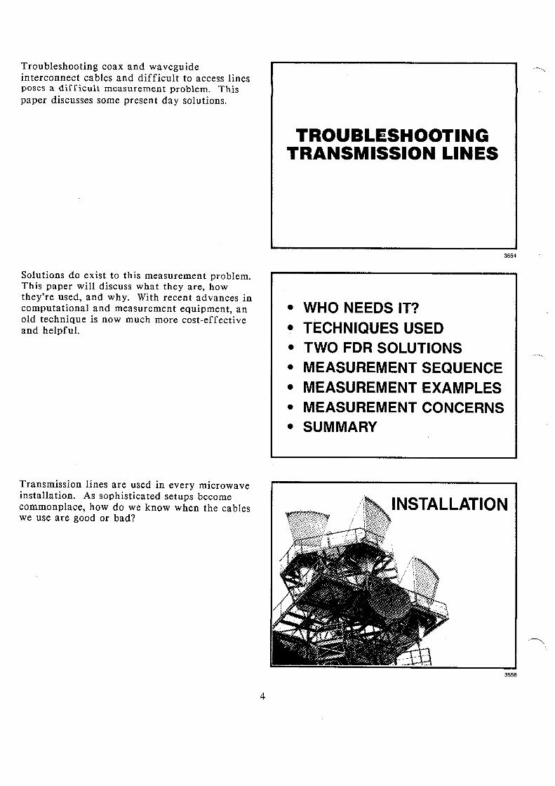
Transmission lines are used in every microwaveinstallation. As sophisticated setups becomecommonplace, how do we know when the cableswe use are good or bad?

4

TROUBLESHOOTINGTRANSMISSION LINES

3554

• WHO NEEDS IT?• TECHNIQUES USED• TWO FDR SOLUTIONS• MEASUREMENT SEQUENCE• MEASUREMENT EXAMPLES• MEASUREMENT CONCERNS• SUMMARY

INSTALLATION

3556

MAINTENANCE

3557

PRODUCTION & INCOMINGINSPECTION

3558

• TECHNIQUES USED

3559

5

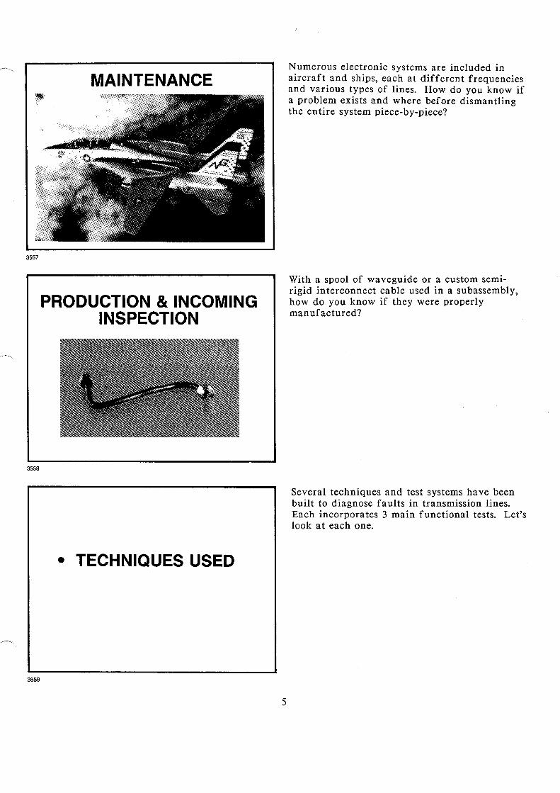
Numerous electronic systems are included inaircraft and ships, each at different frequenciesand various types of lines. How do you know ifa problem exists and where before dismantlingthe entire system piece-by-piece?

With a spool of waveguide or a custom semi­rigid interconnect cable used in a subassembly,how do you know if they were properlymanufactured?

Several techniques and test systems have beenbuilt to diagnose faults in transmission lines.Each incorporates 3 main functional tests. Let'slook at each one.

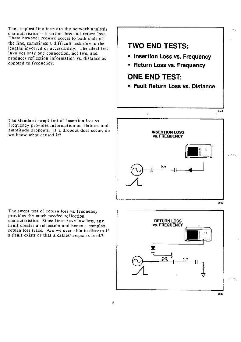
The simplest line tests are the network analysischaracteristics -- insertion loss and return loss.These however require access to both ends ofthe line, sometimes a difficult task due to thelengths involved or accessibility. The ideal testinvolves only one connection, not two, andproduces reflection information vs. distance asopposed to frequency.

The standard swept test of insertion loss vs.frequency provides information on flatness andamplitude dropouts. If a dropout does occur, dowe know what caused it?

The swept test of return loss vs. frequencyprovides the much needed reflectioncharacteristics. Since lines have low loss, anyfault creates a reflection and hence a complexreturn loss trace. Are we ever able to discern ifa fault exists or that a cables' response is ok?

6

TWO END TESTS:

• Insertion Loss vs. Frequency

• Return Loss vs. Frequency

ONE END TEST:• Fault Return Loss vs. Distance

INSERTION LOSSvs. FREQUENCY

•. ~~

,~-- - ~ 000

RET~RN LOSSV5. FflEQUENCY

, • II 0i (ilQao

J

l ~

6J X <'II OUT 11A

3559

3560

3561

FAULT RETURN LOSSvs. DISTANCE

Computer

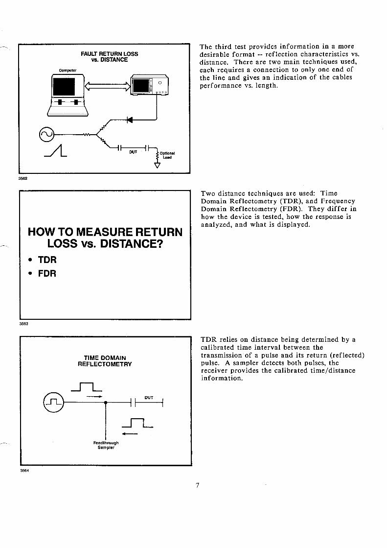
•The third test provides information in a moredesirable format -- reflection characteristics vs.distance. There are two main techniques used,each requires a connection to only one end ofthe line and gives an indication of the cablesperformance vs. length.

3562

rvl----...J\N1..-'-<

A OUT '1OptionalLoad

HOW TO MEASURE RETURNLOSS vs. DISTANCE?

• TOR• FOR

3563

TIME DOMAINREFLECTOMETRY

- lOUTSLJ-----~t----f,1--

-Feedthrough

Sampler

3564

7

Two distance techniques are used: TimeDomain Reflectometry (TDR), and FrequencyDomain Reflectometry (FDR). They differ inhow the device is tested, how the response isanalyzed, and what is displayed.

TDR relies on distance being determined by acalibrated time interval between thetransmission of a pulse and its return (reflected)pulse. A sampler detects both pulses, thereceiver provides the calibrated time/distanceinformation.

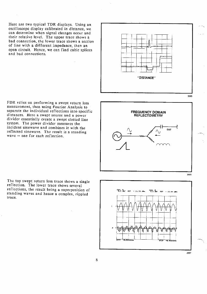
Here are two typical TDR displays. Using anoscilloscope display calibrated in distance, wecan determine when signal changes occur andtheir relative level. The upper trace shows abad connection, the lower trace shows a sectionof line with a different impedance, then anopen circuit. Hence, we can find cable splicesand bad connections.

711\...

r-- j.-J

IL-IJ

"DISTANCE"

3565

FDR relies on performing a swept return lossmeasurement, then using Fourier Analysis toseparate the individual reflections into specificdistances. Here a swept source and a powerdivider essentially create a swept slotted linesystem. The power divider measures theincident sinewave and combines it with thereflected sinewave. The result is a standingwave -- one for each reflection.

FREQUENCY DOMAINREFLECTOMETRY

OUT

3566

CHh B CH2. B5~ 0 dB/ REF - ll~ 72 dBm 5.0 dB/ REF - 10. 88 dam

STOP +8. 6000GHzSTRT 6. 6000GHz

1\ 1\ 1/\ hi (\1(\ V\/t\/ (\ f\IV II ~ V VIV 1/ \ V VIV v\

.•.M .M lilA I\A .1' rJI, ,/\. ~I\, .~

I VVV IVVv IV' .~ 'IN IN lW M'1/\ IN VV IW' 'I

+

2 •

1 •

The top swept return loss trace shows a singlereflection. The lower trace shows severalreflections, the result being a superposition ofstanding waves and hence a complex, rippledtrace.

3567

8

Return

Lossvs.

Freq.

Inverse

FFT

Return

Lossvs.

Distance

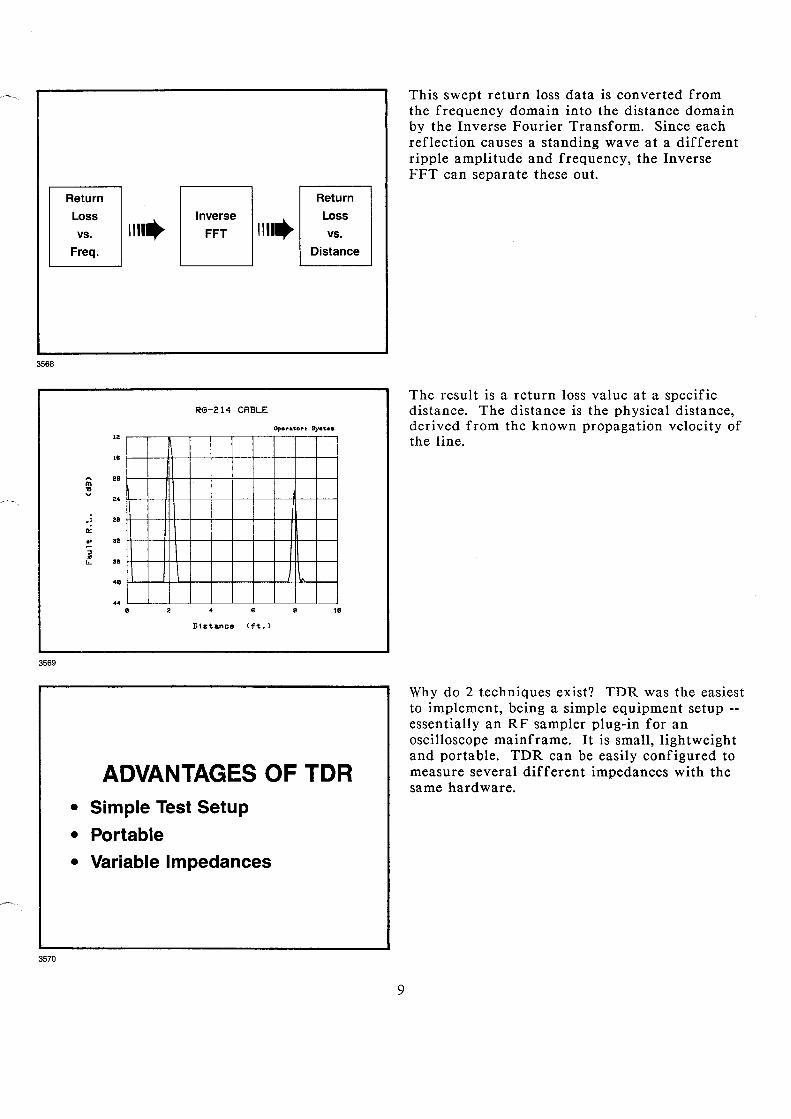
This swept return loss data is converted fromthe frequency domain into the distance domainby the Inverse Fourier Transform. Since eachreflection causes a standing wave at a differentripple amplitude and frequency, the InverseFFT can separate these out.

3568

RG-214 CABLE

0,.,. ..100,.1 By."••,.••

Ii> 28

...v ••~

J 28

~

~82

"" as"-

48

••8 18

Dls'tance (ft. l

3569

ADVANTAGES OF TOR• Simple Test Setup

• Portable• Variable Impedances

3570

9

The result is a return loss value at a specificdistance. The distance is the physical distance,derived from the known propagation velocity ofthe line.

Why do 2 techniques exist? TDR was the easiestto implement, being a simple equipment setup -­essentially an RF sampler plug-in for anoscilloscope mainframe. It is small, lightweightand portable. TDR can be easily configured tomeasure several different impedances with thesame hardware.

Unfortunately, TDR doesn't allow the user totest bandlimited devices like waveguide -- itrequires a broad frequency coverage to transmitthe pulse. Likewise, the accuracy of amplituderesponses is poor. If multiple faults exist, theTDR waveform is complex and difficult todiagnose. FDR overcomes all of theselimitations since the frequency span iscontrollable, plus the system is a broadbandnetwork analyzer.

HP provides two different FDR measurementsystems. They differ in speed, performance,capability, and cost.

ADVANTAGES OF FOR

• Insertion Loss, Return Loss vs.Frequency, plus Return Lossvs. Distance

• Can Test Band Limited Devices

• Multiple Fault Detection

• TWO FOR SOLUTIONS

3571

3555

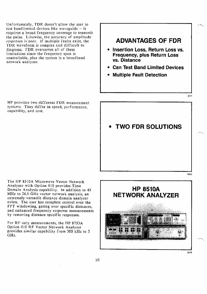
The HP 8510A Microwave Vector NetworkAnalyzer with Option 010 provides TimeDomain Analysis capability. In addition to 45MHz to 26.5 GHz vector network analysis, anextremely versatile distance domain analyzerexists. The user has complete control over theFFT windowing, gating over specific distances,and enhanced frequency response measurementsby removing distance specific responses.

For RF only measurements, the HP 8753AOption 010 RF Vector Network Analyzerprovides similar capability from 300 kHz to 3GHz.

10

HP 8510ANETWORK ANALYZER

3578

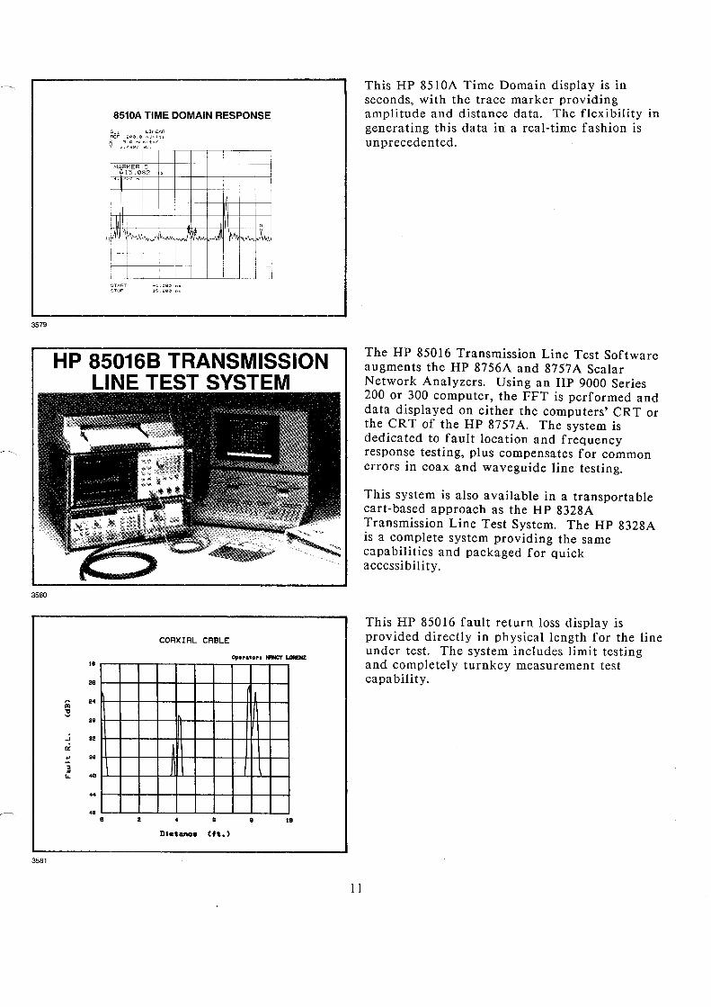
This HP 85l0A Time Domain display is inseconds, with the trace marker providingamplitude and distance data. The flexibility ingenerating this data in a real-time fashion isunprecedented.

8510A TIME DOMAIN RESPONSE

Sl1 LINEARREF -200.0 ,.,Un i t$V 5.0 mU,.,it$/

3.4807 mU.

! !

M RKER 515.0 2 ,

! 4. 2F7 m

! II I,

I, I ! ,-lAI k" PM ,~I \~A x•.

r

I,I

START -1.000 ,..'"STOP 16.200 ,.,'"

3579

HP 850168 TBANSMISSIONLINE TEST SYSTEM

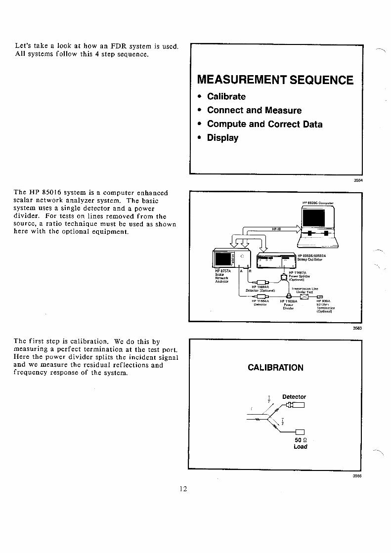
The HP 85016 Transmission Line Test Softwareaugments the HP 8756A and 8757A ScalarNetwork Analyzers. Using an HP 9000 Series200 or 300 computer, the FFT is performed anddata displayed on either the computers' CRT orthe CRT of the HP 8757A. The system isdedicated to fault location and frequencyresponse testing, plus compensates for commonerrors in coax and waveguide line testing.

This system is also available in a transportablecart-based approach as the HP 8328ATransmission Line Test System. The HP 8328Ais a complete system providing the samecapabilities and packaged for quickaccessibili ty.

3580

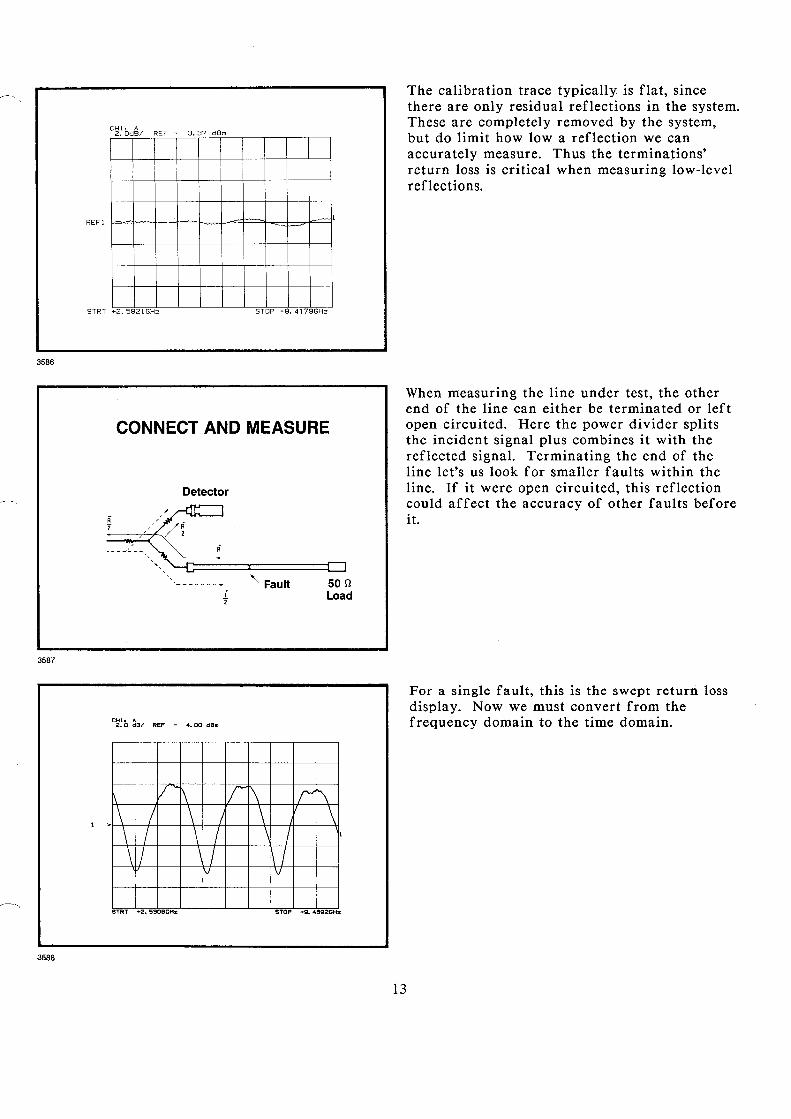
Ope..&'toPI NINC'I LORENZ,.28

Iii 2<

~2.

J 32

Q<

~a.

"" <8lL ..~, ••

CORXIRL CRBLE:

I11

2 8 18

This HP 85016 fault return loss display isprovided directly in physical length for the lineunder test. The system includes limit testingand completely turnkey measurement testcapability.

Dl ..1:ance (f1:.)

3581

11

Let's take a look at how an FDR system is used.All systems follow this 4 step sequence.

MEASUREMENT SEQUENCE• Calibrate

• Connect and Measure

• Compute and Correct Data

• Display

3584

HP 9836C Computer

HP909A50 OhmTermination(Optional)

•Transmission Line

Under Test

HP-IB

~~~~~ HP 8350B/83592ASweep Oscillator

HP 1,664A HP 11636ADetector Power

Divider

The HP 85016 system is a .computer enhancedscalar network analyzer system. The basicsystem uses a single detector and a powerdivider. For tests on lines removed from thesource, a ratio technique milst be used as shownhere with the optional equipment.

3583

The first step is calibration. We do this bymeasuring a perfect termination at the test port.Here the power divider splits the incident signaland we measure the residual reflections andfrequency response of the system.

CALIBRATION

T Detector2

50 aLoad

3585

12

CH1: A2.0dBI REF - 3.37 dBm

The calibration trace typically is flat, sincethere are only residual reflections in the system.These are completely removed by the system,but do limit how Iowa reflection we canaccurately measure. Thus the terminations'return loss is critical when measuring low-levelreflections.

STRT +2. 5821GHz STOP +9. 4179GHz

3586

CONNECT AND MEASURE

Detector

i'2

" Fault

When measuring the line under test, the otherend of the line can either be terminated or leftopen circuited. Here the power divider splitsthe incident signal plus combines it with thereflected signal. Terminating the end of theline let's us look for smaller faults within theline. If it were open circuited, this reflectioncould affect the accuracy of other faults beforeit.

3587

CHh '"2. 0 dB/ REF - 4 e 00 dBm

For a single fault, this is the swept return lossdisplay. Now we must convert from thefrequency domain to the time domain.

STOP .g. "e920HzSTRT 2. 530BGHz

V \ Ir1\ / r\. \ / \ / \ \

\ / \ / \ / 1

\ / / /v v

.

3588

13

The time domain information must be convertedinto distance domain data for physical length.In the process, we must correct for losses in thesystem due to the line characteristics such asattenuation and dispersion, plus multiplemismatches.

COMPUTE ANDCORRECT FOR

• Time to Distance

• Attenuation of Cable

• Multiple Fault Mismatch

• Waveguide Dispersion

3590

Calibrating the time domain to physical distancerequires the line velocity of propagation (Vp).This allows us to scale the equivalent electricallength into physical length. TIME TO DISTANCE

Need:

• Velocity of Propagation

• Coax or Waveguide?

3986

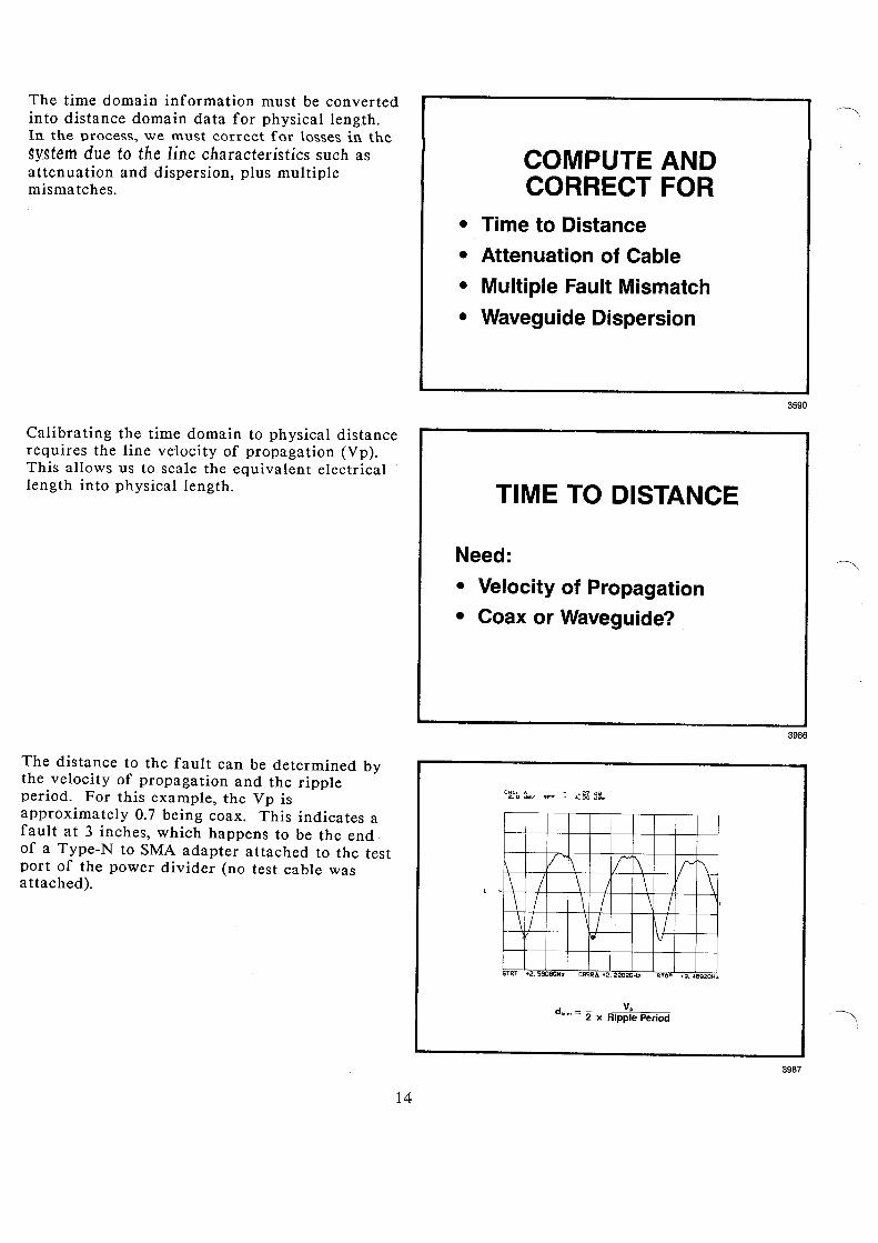
S RT 2. 530BGHz CRSRA 2. 2202CHz STOP Q. 4eg~CHz

CHl1" - .27 dB2. 0 dB/ REF - 4. 00 de",

/ \ r !\ / r\. \ I \ / \ \

\ / \ / \ / 1

\ / / /.. V

T + + +

The distance to the fault can be determined bythe velocity of propagation and the rippleperiod. For this example, the Vp isapproximately 0.7 being coax. This indicates afault at 3 inches, which happens to be the endof a Type-N to SMA adapter attached to the testport of the power divider (no test cable wasattached).

d"",, = 2 X Rip~;e Period

3987

14

LINE ATTENUATION

Since the line has some loss vs. distance, wemust correct for the round trip path loss of eachreflected signal. This is achieved by using theline attenuation for the line under test.

Need:

• Loss per 100 feet/meters

3988

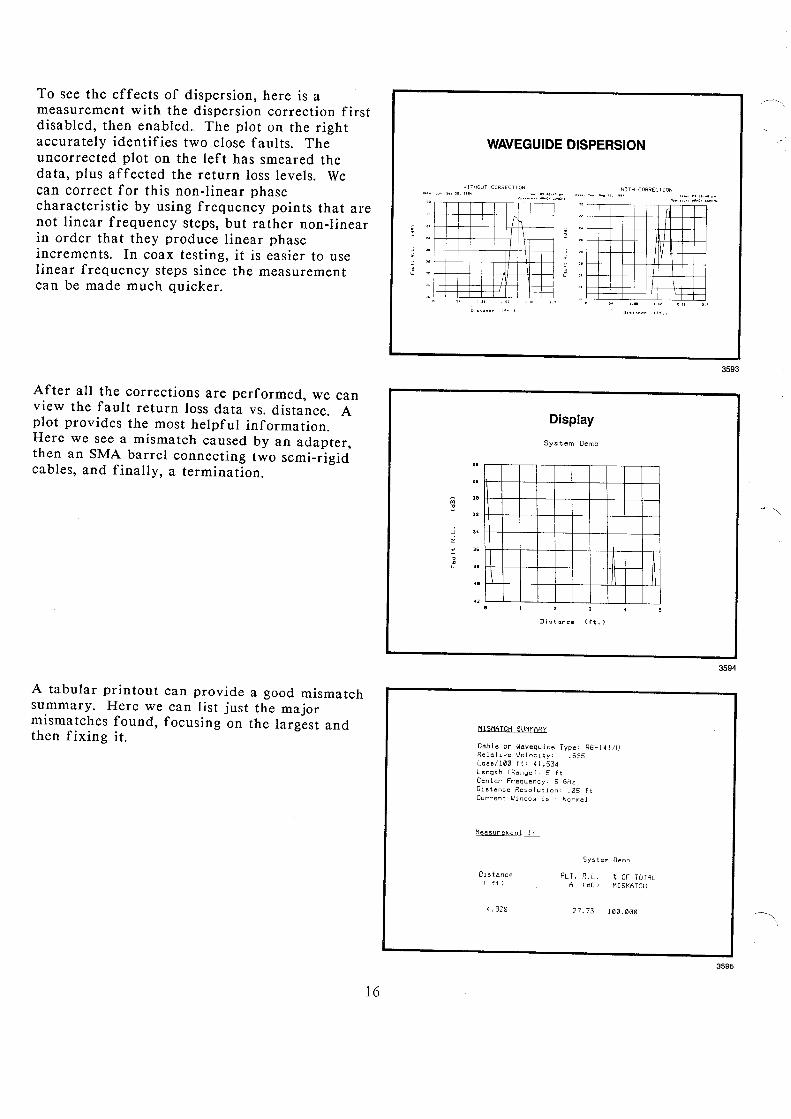
MULTIPLE FAULT MISMATCH

~

1. 0 r------"'--'..:.'--,UncorrectedMagnitude 0.5

Pl' MEAS Pz. I.1EAS

J\ A

If more than one fault exists, the first (andclosest) fault reduces the signal incident to thefollowing faults. This affects the return lossmeasured at each of these faults. Once thepositions of each fault are known, we cancorrect for this mismatch loss and make moreaccurate readings.

d l d ZDISTANCE

CorrectedMagnitude

F, "

tfij_20 lOG Pl- MEAS +----so-

1.0

-20 lOG PZ' MEAS + F ;0 d 2

0.5

-20 lOG ( l-Pt2)

oIII dZ

DISTANCE

3592

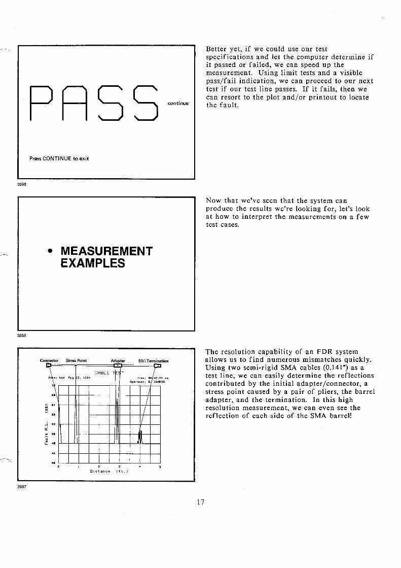
WAVEGUIDE DISPERSIONWhen measuring waveguide, the test algorithmmust be modified to account for the guides'non-linear phase characteristics. As seen in thisexample, the ripple frequency changes goingfrom the low end of the band to the high end.This is because the group delay of the guide isdecreasing with higher frequencies. If weoperate over a narrower portion of the band, wecan ignore this effect. If not, special processingmust be used.

STOP ... 12. OOOGHz

CHll A5 OdS I REF'" 00 dB

~~A ~ I~ AIIAAIfIfI fir1/\ /\ 1/\ A1\ f\ 1\ 1\ {1

1m ~~ ~ ~ ~ ~ n II v V\ i VvIV VVV

+

REFl

STRT 7. OOOOGHz

3996

15

WAVEGUIDE DISPERSION

To see the effects of dispersion, here is ameasurement with the dispersion correction firstdisabled, then enabled. The plot on the rightaccurately identifies two close faults. Theuncorrected plot on the left has smeared thedata, plus affected the return loss levels. Wecan correct for this non-linear phasecharacteristic by using frequency points that arenot linear frequency steps, but rather non-linearin order that they produce linear phaseincrements. In coax testing, it is easier to uselinear frequency steps since the measurementcan be made much quicker.

WITHOUT CORRECTION

r\\\

I

IL..H

WITH CORRECTION

j ,,1-+-+-+-I-+~-4--I-+-I

e "e-+--+--+---je-+-++--l1---ie-+--j~ ,,:-+-t-+--I:-++t--t+-I:-+--1

3593

After all the corrections are performed, we canview the fault return loss data vs. distance. Aplot provides the most helpful information.Here we see a mismatch caused by an adapter,then an SMA barrel connecting two semi-rigidcables, and finally, a termination.

A tabular printout can provide a good mismatchsummary. Here we can list just the majormismatches found, focusing on the largest andthen fixing it.

Display

System Demo

T 11\ 1\

Distance (-{t.)

MISMATCH SUMMARY

Cable or Wavequide Type: RG-1411URelative Velocity: .695L0551l00 ft, 41.534LenQth (Range): 5 ftCenter Frequency: 66HzDistance Resolution: .05 ftCurrent Window is : Nari"'lal

MeasureMent 1:

Systel'1 OerolO

3594

..~

16

Distance( ft)

4.920

FLL R.L, X OF TOTALA (dB) MISMATCH

27.73 100.000

3595

Better yet, if we could use our testspecifications and let the computer determine ifit passed or failed, we can speed up themeasurement. Using limit tests and a visiblepass/fail indication, we can proceed to our nexttest if our test line passes. If it fails, then wecan resort to the plot and/or printout to locatethe fault.

Press CONTINUE to exit

3596

Now that we've seen that the system canproduce the results we're looking for, let's lookat how to interpret the measurements on a fewtest cases.

• MEASUREMENTEXAMPLES

3555

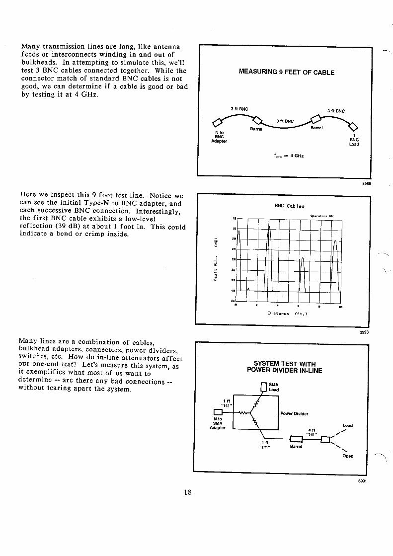
The resolution capability of an FDR systemallows us to find numerous mismatches Quickly.Using two semi-rigid SMA cables (0.141 ") as atest line, we can easily determine the reflectionscontributed by the initial adapter/connector, astress point caused by a pair of pliers, the barreladapter, and the termination. In this highresolution measurement, we can even see thereflection of each side of the SMA barrel!

50.0. TerminationAdapter

CABLE TE Tn •• , .9l~,,,\_. Ru, 2, t9B1

Op.,..t.or: G CONRR

•• f

/../••

1/3 •

..•• }~

..••

JD."

Connector Stress Point

3

Distance (ft.)

3997

17

Many transmission lines are long, like antennafeeds or interconnects winding in and out ofbulkheads. In attempting to simulate this, we'lltest 3 BNC cables connected together. While theconnector match of standard BNC cables is notgood, we can determine if a cable is good or badby testing it at 4 GHz.

MEASURING 9 FEET OF CABLE

3ft BNC 3ft BNC

NtoBNC

Adapter1

BNCload

tOO"'" = 4 GHz

3989

BNC Cables

2

8

8

I4

• "2

I.48

...J

a:

~::J

"4. 38

III..,

Here we inspect this 9 foot test line. Notice wecan see the initial Type-N to BNC adapter, andeach successive BNC connection. Interestingly,the first BNC cable exhibits a low-levelreflection (39 dB) at about I foot in. This couldindicate a bend or crimp inside.

448 4 18

Distance (ft.)

3990

Many lines are a combination of cables,bulkhead adapters, connectors, power dividers,switches, etc. How do in-line attenuators affectour one-end test? Let's measure this system, asit exemplifies what most of us want todetermine -- are there any bad connections -­without tearing apart the system.

SYSTEM TEST WITHPOWER DIVIDER IN-LINE

Load",-

",-

"'".....Barrel ...... ......

Open

3991

18

D.,., T... ~ J .. , '~." To., "",g,,,••_o".,.,~" ""

3992

"

"

:11A1\

.\ \ I

"

"

A

I \ A:\ 1 I A

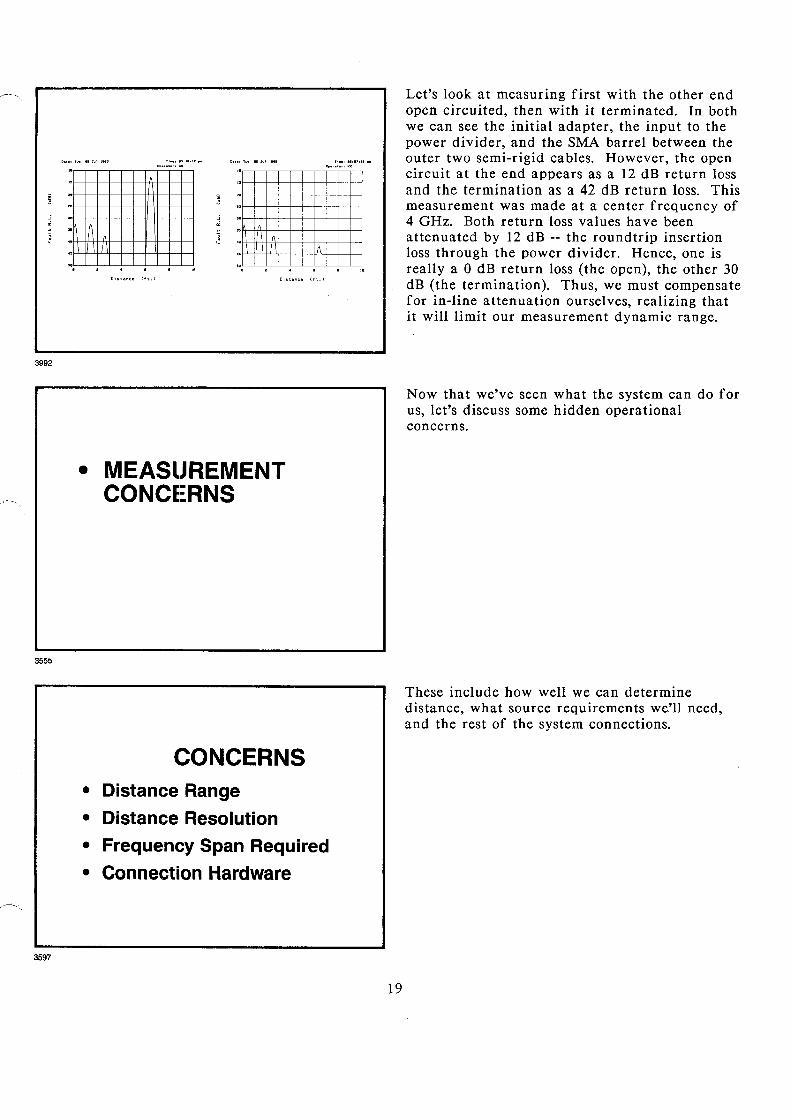
Let's look at measuring first with the other endopen circuited, then with it terminated. In bothwe can see the initial adapter, the input to thepower divider, and the SMA barrel between theouter two semi-rigid cables. However, the opencircuit at the end appears as a 12 dB return lossand the termination as a 42 dB return loss. Thismeasurement was made at a center frequency of4 GHz. Both return loss values have beenattenuated by 12 dB -- the roundtrip insertionloss through the power divider. Hence, one isreally a 0 dB return loss (the open), the other 30dB (the termination). Thus, we must compensatefor in-line attenuation ourselves, realizing thatit will limit our measurement dynamic range.

Now that we've seen what the system can do forus, let's discuss some hidden operationalconcerns.

3555

3597

• MEASUREMENTCONCERNS

CONCERNS• Distance Range

• Distance Resolution

• Frequency Span Required

• Connection Hardware

19

These include how well we can determinedistance, what source requirements we'll need,and the rest of the system connections.

DISTANCE vs. FREQUENCY

Range -

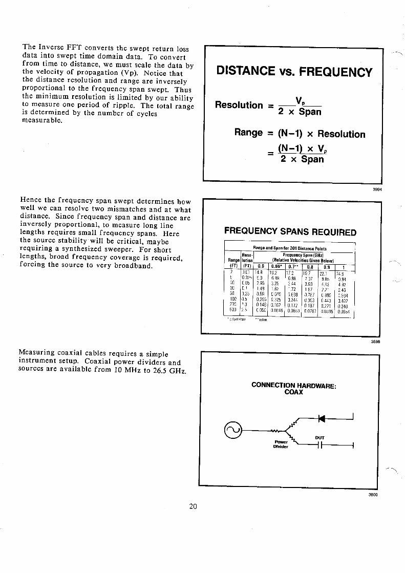
The Inverse FFT converts the swept return lossdata into swept time domain data. To convertfrom time to distance, we must scale the data bythe velocity of propagation (Vp). Notice thatthe distance resolution and range are inverselyproportional to the frequency span swept. Thusthe minimum resolution is limited by our abilityto measure one period of ripple. The total rangeis determined by the number of cyclesmeasurable.

Resolution - 2 x Span

(N -1) x Resolution(N-1) x Vp

2 x Span

3994

Hence the frequency span swept determines howwell we can resolve two mismatches and at whatdistance. Since frequency span and distance areinversely proportional, to measure long linelengths requires small frequency spans. Herethe source stability will be critical, mayberequiring a synthesized sweeper. For shortlengths, broad frequency coverage is required,forcing the source to very broadband.

Measuring coaxial cables requires a simpleinstrument setup. Coaxial power dividers andsources are available from 10 MHz to 26.5 GHz.

20

FREQUENCY SPANS REQUIRED

Range and Span for 201 Distance PointsReso- Frequency Span (6Hz)

Range lution (Relative Velocities Given Below)(FT) (FT) 0.6 0.66' 0.7" 0.8 0.9 12 0.01 14.8 162 172 19.7 22.1 24.65 0025 5.9 649 6.88 787 885 9.8410 0.05 295 325 344 393 443 4.9220 0.1 148 162 1.72 197 221 24650 0.25 0.59 0649 0688 0.787 0.885 0.984100 0.5 0295 0.325 0.344 0.393 0.443 0492200 10 0.148 0162 0172 0.197 0221 0246500 2.5 0059 00649 0.0688 0.0787 00885 00984

"polyethylene ··lellon

CONNECTION HARDWARE:COAX

61-::{ ~ IDivider' iY i

3598

3600

WHY POWER DIVIDER?

3601

Splitter

50/'~50fl

... 831;3fl

Divider

16% fl

16% fl

16% fl

.- 50 fl

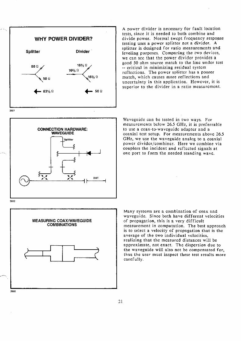
A power divider is necessary for fault locationtests, since it is needed to both combine anddivide power. Normal swept frequency responsetesting uses a power splitter not a divider. Asplitter is designed for ratio measurements andleveling purposes. Comparing the two devices,we can see that the power divider provides agood 50 ohm source match to the line under test-- critical in minimizing residual systemreflections. The power splitter has a poorermatch, which causes more reflections anduncertainty in this application. However, it issuperior to the divider in a ratio measurement.

3602

3995

CONNECTION HARDWARE:WAVEGUIDE-t~5----~

-~ cS~-~X-,--__X_------II ~I_D_UT----I

MEASURING COAX/WAVEGUIDECOMBINATIONS

( C (

Waveguide can be tested in two ways. Formeasurements below 26.5 GHz, it is preferrableto use a coax-to-waveguide adapter and acoaxial test setup. For measurements above 26.5GHz, we use the waveguide analog to a coaxialpower divider jcombiner. Here we combine viacouplers the incident and reflected signals atone port to form the needed standing wave.

Many systems are a combination of coax andwaveguide. Since both have different velocitiesof propagation, this is a very difficultmeasurement in computation. The best approachis to select a velocity of propagation that is theaverage of the two individual velocities,realizing that the measured distances will beapproximate, not exact. The dispersion due tothe waveguide will also not be compensated for,thus the user must inspect these test results morecarefully.

21

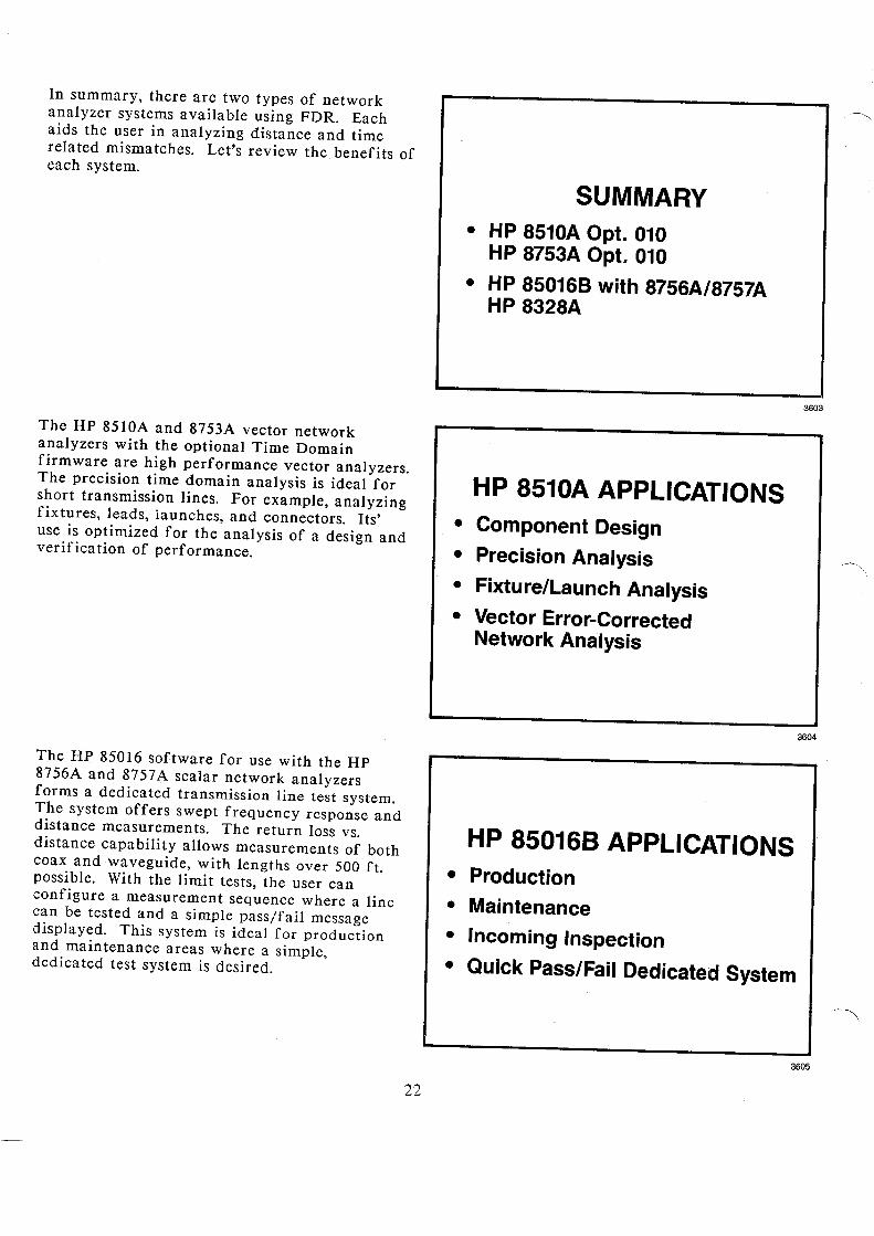
In summary, there are two types of networkanalyzer systems available using FDR. Eachaids the user in analyzing distance and timerelated mismatches. Let's review the benefits ofeach system.

The HP 8510A and 8753A vector networkanalyzers with the optional Time Domainfirmware are high performance vector analyzers.The precision time domain analysis is ideal forshort transmission lines. For example, analyzingfixtures, leads, launches, and connectors. Its'use is optimized for the analysis of a design andverification of performance.

The HP 85016 software for use with the HP8756A and 8757A scalar network analyzersforms a dedicated transmission line test system.The system offers swept frequency response anddistance measurements. The return loss vs.distance capability allows measurements of bothcoax and waveguide, with lengths over 500 ft.possible. With the limit tests, the user canconfigure a measurement sequence where a linecan be tested and a simple pass/fail messagedisplayed. This system is ideal for productionand maintenance areas where a simple,dedicated test system is desired.

22

SUMMARY• HP 8510A Opt. 010

HP 8753A Opt. 010• HP 850168 with 8756A/8757A

HP 8328A

3603

HP 8510A APPLICATIONS• Component Design• Precision Analysis• Fixture/Launch Analysis• Vector Error-Corrected

Network Analysis

3604

HP 850168 APPLICATIONS• Production• Maintenance• Incoming Inspection• Quick Pass/Fail Dedicated System

3605

HP 8328A

3606

REFERENCES

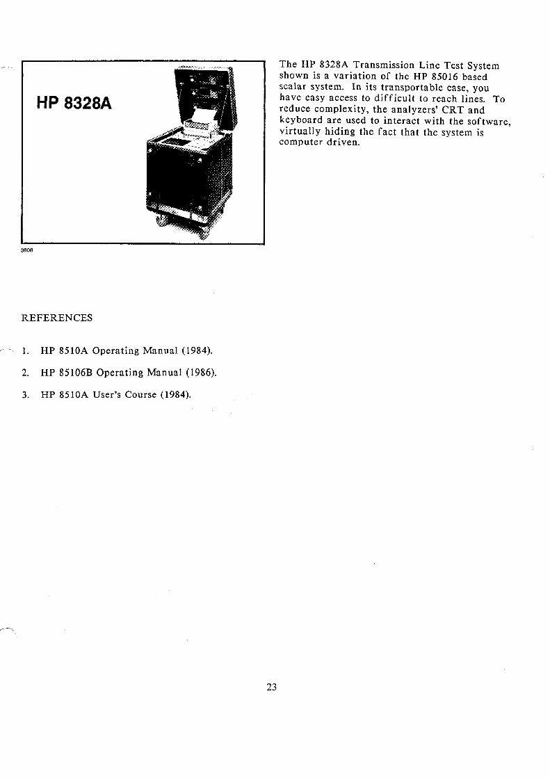
The HP 8328A Transmission Line Test Systemshown is a variation of the HP 85016 basedscalar system. In its transportable case, youhave easy access to difficult to reach lines. Toreduce complexity, the analyzers' CRT andkeyboard are used to interact with the software,virtually hiding the fact that the system iscomputer driven.

1. HP 8510A Operating Manual (1984).

2. HP 85106B Operating Manual (1986).

3. HP 8510A User's Course (1984).

23

HEWLETTPACKARD

5954-1545 August 1985 Printed in U.S.A.