Embed Size (px)
Citation preview
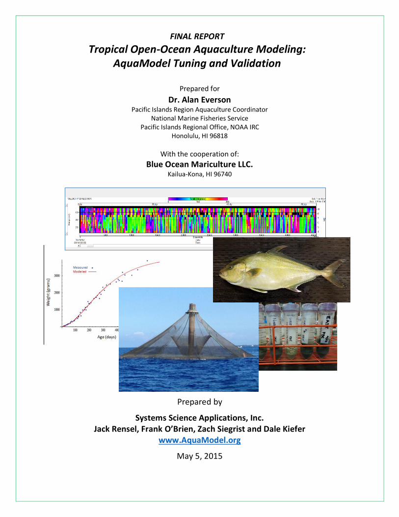
Prepared for
Dr. Alan Everson Pacific Islands Region Aquaculture Coordinator
National Marine Fisheries Service Pacific Islands Regional Office, NOAA IRC
Honolulu, HI 96818
With the cooperation of:
Blue Ocean Mariculture LLC. Kailua-Kona, HI 96740
Prepared by
Systems Science Applications, Inc. Jack Rensel, Frank O’Brien, Zach Siegrist and Dale Kiefer
www.AquaModel.org
May 5, 2015
FINAL REPORT Tropical Open-Ocean Aquaculture Modeling:
AquaModel Tuning and Validation
Tropical Open-Ocean Aquaculture Modeling: AquaModel Tuning and Validation ii
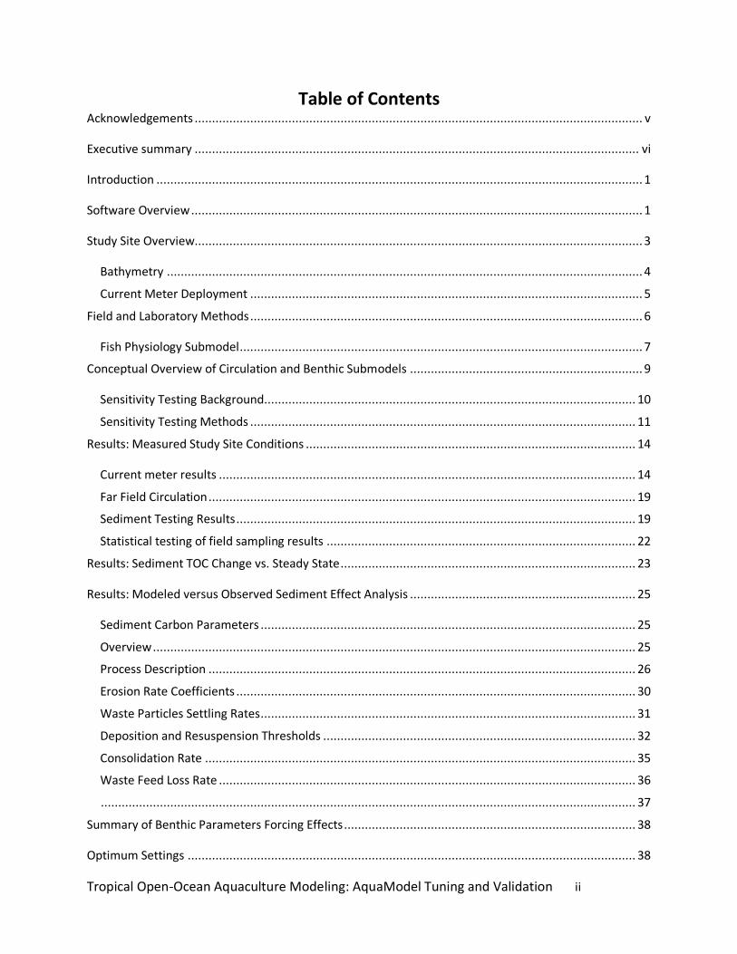
Table of Contents
Acknowledgements ................................................................................................................................. v
Executive summary ................................................................................................................................ vi
Introduction ............................................................................................................................................ 1
Software Overview .................................................................................................................................. 1
Study Site Overview................................................................................................................................. 3
Bathymetry ......................................................................................................................................... 4
Current Meter Deployment ................................................................................................................. 5
Field and Laboratory Methods ................................................................................................................. 6
Fish Physiology Submodel .................................................................................................................... 7
Conceptual Overview of Circulation and Benthic Submodels ................................................................... 9
Sensitivity Testing Background........................................................................................................... 10
Sensitivity Testing Methods ............................................................................................................... 11
Results: Measured Study Site Conditions ............................................................................................... 14
Current meter results ........................................................................................................................ 14
Far Field Circulation ........................................................................................................................... 19
Sediment Testing Results ................................................................................................................... 19
Statistical testing of field sampling results ......................................................................................... 22
Results: Sediment TOC Change vs. Steady State ..................................................................................... 23
Results: Modeled versus Observed Sediment Effect Analysis ................................................................. 25
Sediment Carbon Parameters ............................................................................................................ 25
Overview ........................................................................................................................................... 25
Process Description ........................................................................................................................... 26
Erosion Rate Coefficients ................................................................................................................... 30
Waste Particles Settling Rates ............................................................................................................ 31
Deposition and Resuspension Thresholds .......................................................................................... 32
Consolidation Rate ............................................................................................................................ 35
Waste Feed Loss Rate ........................................................................................................................ 36
.......................................................................................................................................................... 37
Summary of Benthic Parameters Forcing Effects .................................................................................... 38
Optimum Settings ................................................................................................................................. 38

Tropical Open-Ocean Aquaculture Modeling: AquaModel Tuning and Validation iii
AquaModel Screen Prints ...................................................................................................................... 39
Summary ............................................................................................................................................... 46
Literature Cited ..................................................................................................................................... 47
Appendix A Pen numbering system, volume, conversion to cubic geometric space and geo-position of cage center. ....................................................................................................................................... 49
Appendix B TOC Laboratory Protocols University of Hawaii Hilo. ...................................................... 49
Appendix C. Table of more important single and multiple factor validation results shown in charts in this document. .................................................................................................................................. 50
Appendix D. List of simulation settings assessed in later part of validation study and resulting skill of model to fit a mean of 0.15% sediment TOC at the center of lease area of Blue Ocean Mariculture. .. 53
Appendix E. List of simulation settings assessed in later part of validation study and resulting skill of model to fit a mean of 0.16% sediment TOC at the center of lease area of Blue Ocean Mariculture. .. 60
Table of Figures Figure 1. Annotated screen print of final minutes of the Blue Ocean Mariculture AquaModel simulation. Light blue and green areas indicate extremely minor increased total organic carbon concentrations. ....viii Figure 2. Conceptual model overview of AquaModel software. .............................................................. 2 Figure 3. Example snapshot in a streaming video-like output of AquaModel showing oxygen use during a low flow period by fish in a fish farm in British Columbia. ........................................................................ 3 Figure 4. Vicinity map (inset) and area map of fish farm lease near Keahole Point, Hawaii after Blue Ocean Mariculture (2014). ....................................................................................................................... 4 Figure 5. Modeling domain (blue/green rectangle) and study locations cited in this report. ................... 5 Figure 6. Photograph of Seriola rivoliana grown at the subject fish farm. ................................................ 7 Figure 7. Measured growth of Seriola rivoliana at Blue Ocean Mariculture net pens compared to modeled growth with no feed, oxygen, and temperature or non-optimal water current velocity limitations. .............................................................................................................................................. 8 Figure 8. Calculated and modeled effect of water temperature on Seriola rivoliana specific growth rate in culture at the Blue Ocean Mariculture net pen facility. ........................................................................ 8 Figure 10. Mean and standard deviation of current velocity at the center of each depth bin. ............... 15 Figure 11. Velocity plot for the entire current meter deployment period (across the image, above), an excerpted section from ensemble 1000 to 2000 (about 25 to 45% through the entire deployment) and a plot of velocity magnitude for bins 5 and 6, (mid depth, the line plot at the bottom). ............................ 16 Figure 12. Direction (True) plot for the entire current meter deployment period with the compass scale shown above from purple, to blue, green yellow, yellow, red and back to purple describing the 360-degree range. ........................................................................................................................................ 17 Figure 13. AquaModel current vector rose for one and two month’s elapsed time at net pen depth. .... 18 Figure 14. AquaModel current vector rose for one and two month’s elapsed time near sea bottom. .... 18 Figure 15. Dried sediment sample from project site in laboratory aluminum container about to be further processed. ................................................................................................................................. 20 Figure 16. Sediment samples from the projectc site being prepared for TOC analysis. .......................... 21 Figure 17. Time series plot of sediment TOC at center of net pen area in one of the better fitting simulation outcomes (Run No. 126). ...................................................................................................... 23
Tropical Open-Ocean Aquaculture Modeling: AquaModel Tuning and Validation iv
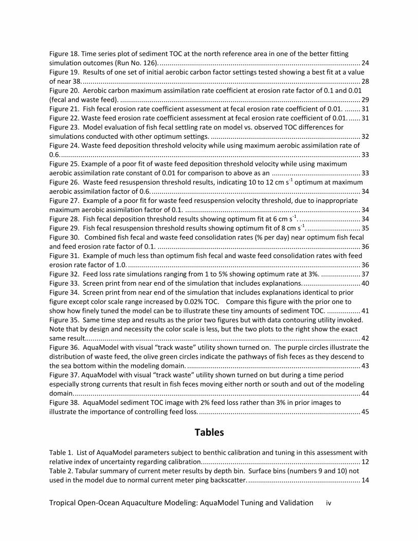
Figure 18. Time series plot of sediment TOC at the north reference area in one of the better fitting simulation outcomes (Run No. 126). ...................................................................................................... 24 Figure 19. Results of one set of initial aerobic carbon factor settings tested showing a best fit at a value of near 38. ............................................................................................................................................. 28 Figure 20. Aerobic carbon maximum assimilation rate coefficient at erosion rate factor of 0.1 and 0.01 (fecal and waste feed). .......................................................................................................................... 29 Figure 21. Fish fecal erosion rate coefficient assessment at fecal erosion rate coefficient of 0.01. ........ 31 Figure 22. Waste feed erosion rate coefficient assessment at fecal erosion rate coefficient of 0.01. ...... 31 Figure 23. Model evaluation of fish fecal settling rate on model vs. observed TOC differences for simulations conducted with other optimum settings. ............................................................................ 32 Figure 24. Waste feed deposition threshold velocity while using maximum aerobic assimilation rate of 0.6. ........................................................................................................................................................ 33 Figure 25. Example of a poor fit of waste feed deposition threshold velocity while using maximum aerobic assimilation rate constant of 0.01 for comparison to above as an ............................................. 33 Figure 26. Waste feed resuspension threshold results, indicating 10 to 12 cm s-1 optimum at maximum aerobic assimilation factor of 0.6. .......................................................................................................... 34 Figure 27. Example of a poor fit for waste feed resuspension velocity threshold, due to inappropriate maximum aerobic assimilation factor of 0.1. ......................................................................................... 34 Figure 28. Fish fecal deposition threshold results showing optimum fit at 6 cm s-1. ............................... 34 Figure 29. Fish fecal resuspension threshold results showing optimum fit of 8 cm s-1. ........................... 35 Figure 30. Combined fish fecal and waste feed consolidation rates (% per day) near optimum fish fecal and feed erosion rate factor of 0.1. ....................................................................................................... 36 Figure 31. Example of much less than optimum fish fecal and waste feed consolidation rates with feed erosion rate factor of 1.0. ...................................................................................................................... 36 Figure 32. Feed loss rate simulations ranging from 1 to 5% showing optimum rate at 3%. .................... 37 Figure 33. Screen print from near end of the simulation that includes explanations. ............................. 40 Figure 34. Screen print from near end of the simulation that includes explanations identical to prior figure except color scale range increased by 0.02% TOC. Compare this figure with the prior one to show how finely tuned the model can be to illustrate these tiny amounts of sediment TOC. ................. 41 Figure 35. Same time step and results as the prior two figures but with data contouring utility invoked. Note that by design and necessity the color scale is less, but the two plots to the right show the exact same result............................................................................................................................................ 42 Figure 36. AquaModel with visual “track waste” utility shown turned on. The purple circles illustrate the distribution of waste feed, the olive green circles indicate the pathways of fish feces as they descend to the sea bottom within the modeling domain. ........................................................................................ 43 Figure 37. AquaModel with visual “track waste” utility shown turned on but during a time period especially strong currents that result in fish feces moving either north or south and out of the modeling domain. ................................................................................................................................................. 44 Figure 38. AquaModel sediment TOC image with 2% feed loss rather than 3% in prior images to illustrate the importance of controlling feed loss. .................................................................................. 45
Tables Table 1. List of AquaModel parameters subject to benthic calibration and tuning in this assessment with relative index of uncertainty regarding calibration. ................................................................................ 12 Table 2. Tabular summary of current meter results by depth bin. Surface bins (numbers 9 and 10) not used in the model due to normal current meter ping backscatter. ......................................................... 14

Tropical Open-Ocean Aquaculture Modeling: AquaModel Tuning and Validation v
Table 3. Mean or single value results for each sampling location by year for surficial sediment total organic carbon samples collected near Blue Ocean Mariculture and in remote reference stations. ........ 20 Table 4. Summary of the effects of key variable modifications upon predicted sediment TOC results in AquaModel. .......................................................................................................................................... 38 Table 5. Optimum settings in order of relative accuracy ranking. See Appendix D for entire list. ...... 39 Table 6. Optimum parameter settings for AquaModel benthic submodel in Hawai’i. ........................... 39
Acknowledgements
This research study was funded in part by a small grant from the National Oceanic and Atmospheric Administration contract AB-133F-13-SE-1447 to Science Systems Applications, Inc. The host company was Blue Ocean Mariculture, Inc. with current meter deployment and recovery coordination and assistance provided by Jennica Lowell, the company’s Research Manager. Company divers assisted in current meter recovery along with site manager Lance Hubbert. The principal investigators were Alan Everson, NOAA Regional Aquaculture Coordinator who was responsible for project administration and Jack Rensel, contractor for System Science Applications who was responsible for project planning and execution, data analysis, model testing, bug identification and report production with assistance from Zach Siegrist. Frank O’Brien provided extensive software code writing for new model utilities and bug fixes. These new utilities will be featured in upcoming reports and web site postings. Dale Kiefer provided Mathematica analysis to assist in model bug correction and constructed the fish submodel. Assistance with digital shoreline preparation was provided by Ken Riley, of the NOAA National Ocean Service, Beaufort NC laboratory. For more information about AquaModel, please visit www.AquaModel.org and the underlying GIS system visit www.runEASy.com
Copyright: No part of this document is to be copied, extracted or used without express written permission of the authors, Science System Applications Inc. or the National Marine Fisheries Service, Honolulu Hawai’i. Citations Guidance: Please cite this document as: Rensel, J.E., F.J. O’Brien Z. Siegrist and D.A. Kiefer. 2015. Tropical Open-Ocean Aquaculture Model Tuning and Validation. Prepared for A. Everson, National Marine Fisheries Service, Honolulu HI, and the National Oceanic and Atmospheric Administration. Prepared by System Science Applications, Inc. 66 p.
Tropical Open-Ocean Aquaculture Modeling: AquaModel Tuning and Validation vi
Executive summary
Performance assessment, regional tuning and validation of a software program known as AquaModel were the primary goals of this study. The software was designed for use by governments and industry to predict the sea bottom and water column effects of fish aquaculture. From an industry perspective, it also includes advanced tools to optimize fish production by obviating the usual trial and error method of configuring pen spacing and loading, by estimating optimum fish loading and culture density for growth in relation to currents and ambient oxygen supply.
The benthic submodel of AquaModel software was applied, tuned and validated at the Blue Ocean Mariculture LLC fish farm site near Kona on the big island of Hawai’i (herein “study site”). Fish production is relatively small at present and this factor, combined with the deep water location and moderately strong current velocity and variable directions of flow allows the organic wastes from the farm to be spread over a very large area and readily assimilated into the food web without perturbations. Seven years of field data from five locations was collected by an independent scientist who reports to the State of Hawaii government for this study. To more accurately simulate the fish farm waste production, AquaModel staff created the first physiological and growth model of the cultured fish, Seriola rivoliana (aka KampachiTM or Almaco jack) and tuned this submodel to produce the same growth patterns and food conversion ratios seen at the study site.
Model Overview
AquaModel is composed of interlinked submodels of fish physiology, hydrodynamics, water/sediment quality, solids dispersion and assimilation into the aquatic food web. The model simultaneously calculates and displays a time series of water and sediment quality conditions resulting from fish feed ingestion, fish growth, respiration, excretion, and egestion. The user is presented with a 3-dimensional video-like simulation of growth, metabolic activity of caged fish, associated flow and transformation of nutrients, oxygen, and particulate wastes in adjacent waters and sediments. The software is used by government managers and researchers in several locations worldwide and is presently being formally validated in Canada and Chile at five large fish farms. These validation activities have necessitated numerous upgrades and new utilities in AquaModel, some that are described herein.
New Fish Submodel
Solid wastes dynamics in the model are calculated from feed consumed and a small percent of waste, as well as the assimilation efficiency and food conversion ratio. These results were compared to measurements and estimates from the fish farmers as a quality assurance measure. A physiological model of the cultured fish species reared at Blue Ocean Mariculture (Seriola rivoliani, aka “KampachiTM”) was created for this project and tested to produce growth and food conversion efficiency results similar to that achieved at the farm site.
Circulation of Study Site and Prior Monitoring Results
Accuracy of aquaculture models is strongly related to the quality of the physical oceanographic inputs, particularly in open ocean conditions where non-tidal forcing factors result in considerable variation of flow rates and directions. Two months of continuous surface to bottom (ADCP) current meter records were collected every 20 minutes at the center of the net pen area lease. Surface currents above submerged net pen depth were strong, averaging about 28 cm s-1, but these subsurface readings were affected to some degree by backscatter from the water-air interface. Reliable current velocity readings were obtained from about 10 meters depth (top of submerged net-pen depth and below) to a few meters above the bottom averaging about 9 to 13 cm s-1 (SD range 7 – 9 cm s-1). Polar current vector
Tropical Open-Ocean Aquaculture Modeling: AquaModel Tuning and Validation vii
diagrams produced by AquaModel indicated good dispersion flows in all directions with dominance to the northeast and southwest at net-pen depth and flowing mainly to north and south nearest the sea bottom. These characteristics indicate suitable conditions for rearing fish and provide regular resuspension of solid wastes on the sea bottom. Resuspension allows for aerobic assimilation of the waste feed and fish feces.
The sea bottom was composed of a thin, coarse-sand layer over hardpan and had very low background (reference station) total organic carbon concentrations (TOC) of about 0.14% (SD = 0.03) as measured over several years of monitoring. There were four reference areas sampled and one near-net-pen location from the center of the aquatic lease area. Field data suggested only a possible increase of about 0.1 to 0.2 %TOC near the center of the net pen locations to values of 0.15 or 0.16 %TOC (SD = 0.05), respectively. Statistical difference (p =0.035, df =6) was found comparing sediment TOC results of annual mean from a reference area to the center of the net pen area. No field data were available from sediments immediately adjacent to the net pens but the model produced estimates for all locations.
Modeling Challenge
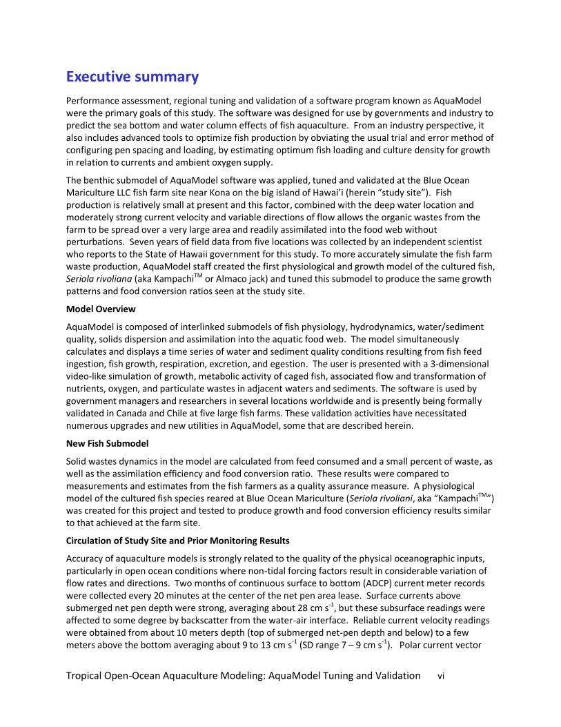
Because of the naturally low organic carbon content of the sea bottom and the relatively small size of the fish farm and the limitations of a single net pen area sampling location, it was not certain at the outset that the model could produce reasonable results. Typically, aquaculture models are used at or for planning of fish farms that may be much larger than the Blue Ocean Mariculture project. Most other farms are located in shallower water, sometimes with lesser current velocity and this produces a strong benthic-effects signal. Therefore, the signal to noise ratio is high for these other farms, but low by a factor of about 5 to 10 or more for the study site. The model was set up to grow concurrent crops of KampachiTM in each cage to a total fish biomass of 590 metric tons, slightly exceeding previous annual production. Figure 1 illustrates one of thousands of frames of the video-like output that the model produces. This one is from near the end of the fish production simulation with maximum fish biomass. The color scale in Figure 1 was adjusted to show an extremely low range of TOC concentrations. Solid green color indicates values of about 0.18 %TOC or about 0.04 %TOC above background, a difference that is similar to the normal error range of a high-precision laboratory analysis.
Model Performance
After calibrating and tuning the AquaModel to regional conditions, it produced background (reference) conditions within >0.001 %TOC of measured, steady-state reference-station values. This is essentially no difference between modeled and measured and certainly not with respect to measurable outcomes in the field. This is noteworthy as other benthic aquaculture models have been unable to maintain background organic carbon steady state concentrations due to resuspension washing TOC out of their modeling domains. With AquaModel, best estimates of the results at the single sampling station nearest the net pens were within<0.0012 %TOC of measured, long-term average results for the best-tuned setup. AquaModel consistently produced slightly higher sediment TOC concentration estimates (<0.02% TOC) at other locations nearer the two largest pens that had no corresponding field data measurements to verify the model predictions at these locations. All of the >250 simulations performed for this study indicated the same spatial pattern of increased TOC, with differing values depending on the calibration settings. None of the TOC concentrations measured or modeled indicated any risk of sea bottom eutrophication or probable significant biological change.

Tropical Open-Ocean Aquaculture Modeling: AquaModel Tuning and Validation viii
Figure 1. Annotated screen print of final minutes of the Blue Ocean Mariculture AquaModel simulation. Light blue and green areas indicate extremely minor increased total organic carbon concentrations.

Tropical Open-Ocean Aquaculture Modeling: AquaModel Tuning and Validation ix
Validation Outcome
This study indicates that the tuned and validated AquaModel program should be sufficiently robust to model other open ocean locations of the leeward shores of the Hawai’ian Islands. The model is designed to work effectively with much higher levels of sediment organic carbon loading from fish farms, but not at grossly eutrophic cage sites in some sheltered, inshore cage locations utilized decades ago. AquaModel use would readily identify such outcomes through observation of several parameters, such as TOC delivery rate to the bottom (“TOC Rate”, in grams carbon per m2 per day) as well as sediment interstitial oxygen and sediment sulfides results. With separate cages that are spaced appropriately, most open ocean locations on the leeward shores of the Hawai’ian Islands that are in sufficient depth of water would not produce eutrophic or even modestly elevated sediment conditions. However, some habitats are considered of special biological significance, where net pen siting should not be considered.
Overview and AquaModel Use in Hawai’i
This evaluation, along with the existing routine monitoring program at the subject site as well as other analyses cited herein, indicate that the fish farm operation is not adversely affecting benthic conditions in the area. The waste tracking utilities of AquaModel applied to this particular site indicate that a small fraction of the waste fish feces reaches locations outside the modeling domain. The estimated loading rate of organic carbon in those locations are so minimal at present that it produces no measurable or even modeling-predicted change in concentration of sediment TOC. The chance of changing the biology of the benthos at these same locations is therefore highly unlikely. In general, small amounts of TOC added to the sea bottom from any source in the marine environment have been found to increase biodiversity and abundance of benthic organisms, but often at nearshore fish farms, these levels are exceeded. AquaModel provides a convenient and relatively accurate means of estimating future carrying capacity for this farm or groups of farms in the future. It also should be used to inform future monitoring efforts, rather than selecting sampling locations through best guess or randomly. Now that regional tuning is complete, configuring and running the model is not difficult for other locations similar to the west coast of the Big Island of Hawai’i and in other similar habitats throughout the region.
AquaModel validation continues at other sites around the world that are larger in fish biomass and more replete with measurement locations in the field. Optimum model calibrations or trends identified in this study were in many cases as expected and occurred in other model validation locations. These findings, combined with prior model use experience and published literature guidance gives us confidence that the validation procedure employed herein is not a product of simple coincidence.

Tropical Open-Ocean Aquaculture Modeling: AquaModel Tuning and Validation 1
Introduction
This report was prepared to summarize results of an AquaModel software validation and regional tuning study conducted in 2013-2014 at an existing open ocean (aka, “offshore”) fish farm site near Kona on the Big Island of Hawai’i. AquaModel has previously been applied in this region of Hawaii by our team, but was focused on theoretical individual net pen sites as well as the consideration of multiple fish farm cumulative effects (O’Brien et al. 2011). The software has been applied to theoretical sites in many different ecoregions around the world and was tuned to local conditions to the extent possible in the past. Some of these studies are reported at www.AquaModel.org on the publications page.
Software Overview
AquaModel is a computational tool for planning and evaluating proposed aquaculture sites, acquiring permits, and assessing investment risks and opportunities. It runs on a standard PC and provides a simple interface to enter environmental and operational information. Graphical outputs map the distribution over time of key parameters including oxygen, particulate organic and dissolved nutrient wastes and dozens or other environmental and fish cultural/management parameters. There are hundreds of pages of model description and examples of simple or complex applications available at the AquaModel website on the publications page. This overview is highly simplified and cursory.
AquaModel is a simulation program that provides for assessment of both farm operations and their environmental effects on coastal or offshore waters. The model describes the nutrient transformations by fish farms of both dissolved and particulate materials in the water column and sea bottom.
A system of equations describe fish growth and physiology that integrates with flow field data to transport waste from farms, assimilate dissolved nutrients by plankton, and simulate the sinking, deposition, resuspension and mineralization of fish feces and uneaten feed. A mathematical description of fish growth and metabolism consists of a nutrient budget for carbon, oxygen, and nitrogen as determined by the size of the fish, water temperature, oxygen concentration, swimming speed, feed rate and composition. Optimal feeding rates for varying environmental conditions are provided as outputs in addition to all other simulation output data in tabular form.
AquaModel provides a dynamic 4-dimensional display (3 dimensions of space plus time = 4D) of aquaculture and environmental processes and resides within our EASy Geographic Information System. This GIS was specifically designed for marine applications and provides interfaces to import diverse types of environmental data including satellite imagery, current meter data, modeled 3-D current data, bathymetry, and coastlines allowing site or regional-specific information to be incorporated into the simulations.
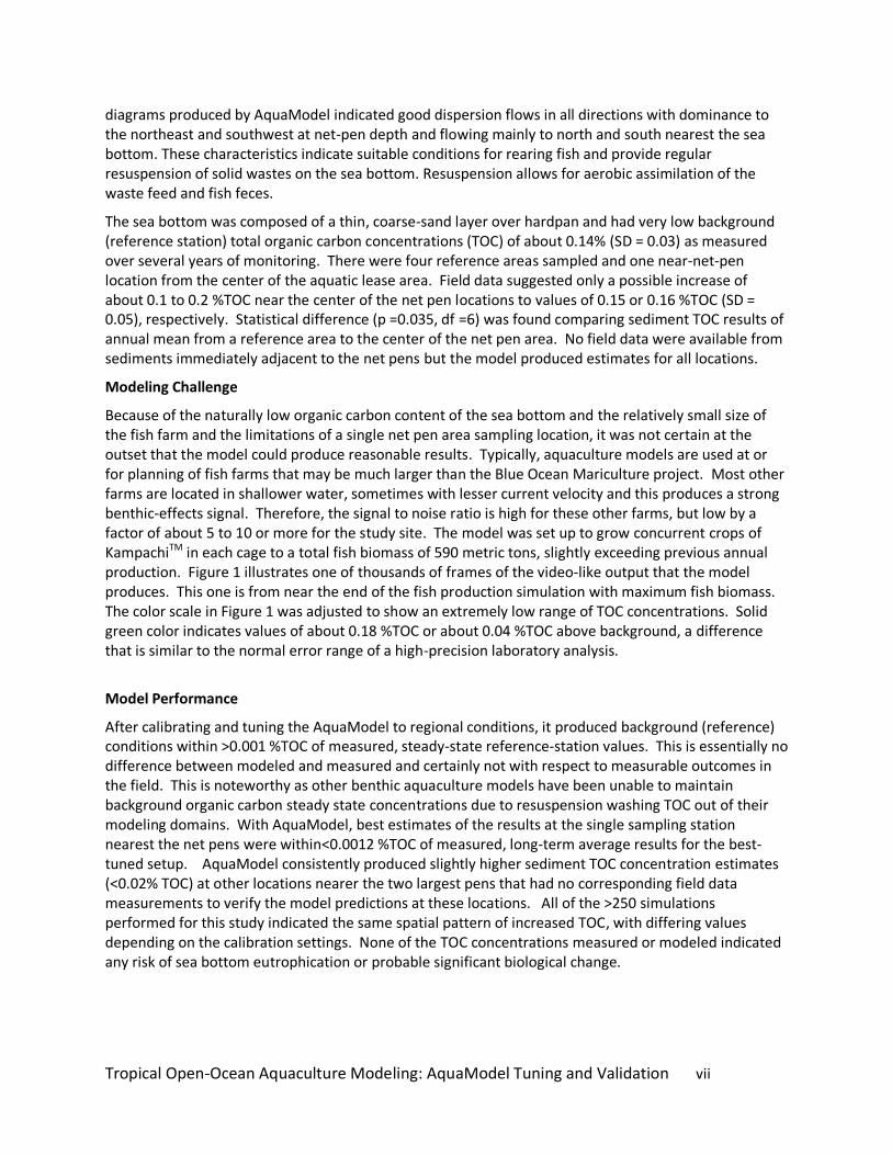
A conceptual representation of major components of AquaModel is shown in Figure 2.
Tropical Open-Ocean Aquaculture Modeling: AquaModel Tuning and Validation 2
Dynamic Fish
Physiology
SubModel
Water SurfaceFeed
Oxygen
Transfer
O2
Soluble
Nutrient
Waste
Wa
ste
Fe
ed
Zooplankton
Phytoplankton
Grazing Recycling
Egestion
Photosynthesis
Sea Bottom
Harvest
(Tissue C, N & P)
Deposition
POC resuspension/transport/oxidation
Aerobic Layer
Human &
Natural
Sources
Anaerobic Layer
2D & 3D
Circulation
SubModel
Fis
h F
ec
es
Suspended
Layer
CO2
Light
Consolidation
Figure 2. Conceptual model overview of AquaModel software.
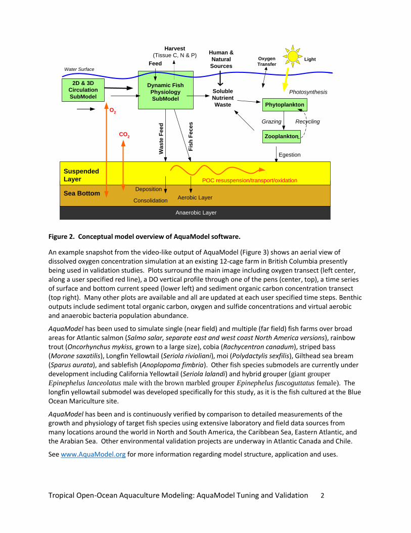
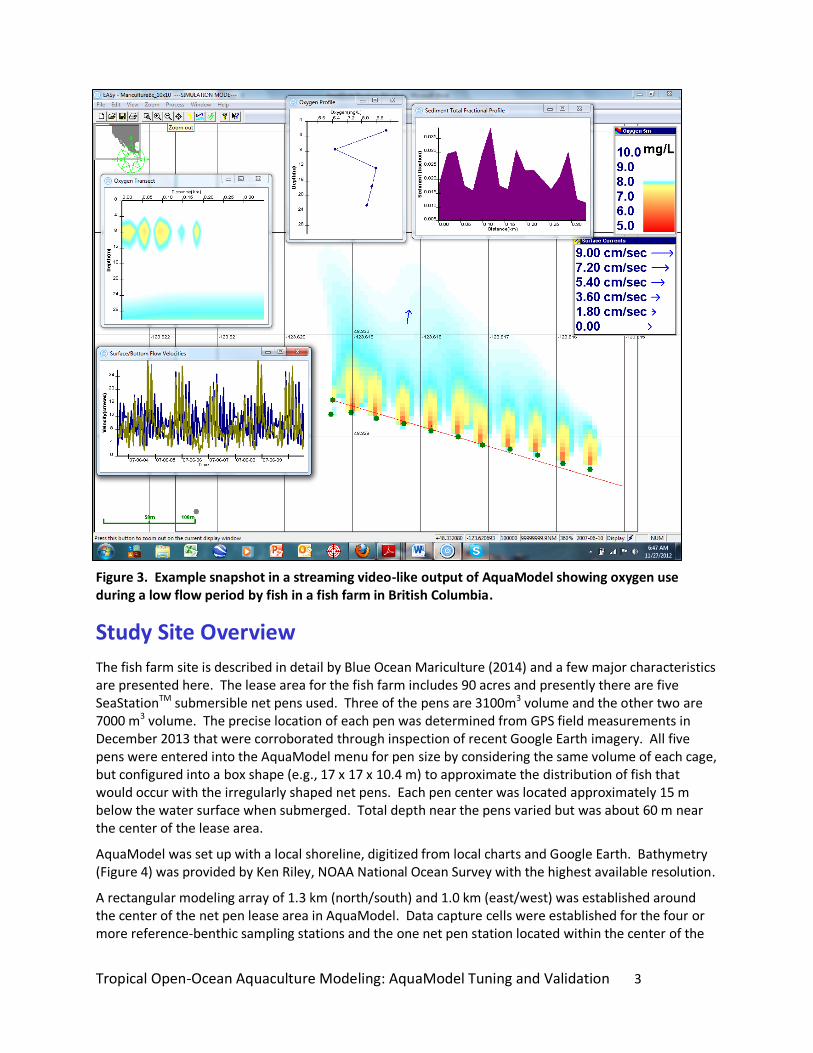
An example snapshot from the video-like output of AquaModel (Figure 3) shows an aerial view of dissolved oxygen concentration simulation at an existing 12-cage farm in British Columbia presently being used in validation studies. Plots surround the main image including oxygen transect (left center, along a user specified red line), a DO vertical profile through one of the pens (center, top), a time series of surface and bottom current speed (lower left) and sediment organic carbon concentration transect (top right). Many other plots are available and all are updated at each user specified time steps. Benthic outputs include sediment total organic carbon, oxygen and sulfide concentrations and virtual aerobic and anaerobic bacteria population abundance.
AquaModel has been used to simulate single (near field) and multiple (far field) fish farms over broad areas for Atlantic salmon (Salmo salar, separate east and west coast North America versions), rainbow trout (Oncorhynchus mykiss, grown to a large size), cobia (Rachycentron canadum), striped bass (Morone saxatilis), Longfin Yellowtail (Seriola rivioliani), moi (Polydactylis sexfilis), Gilthead sea bream (Sparus aurata), and sablefish (Anoplopoma fimbria). Other fish species submodels are currently under development including California Yellowtail (Seriola lalandi) and hybrid grouper (giant grouper
Epinephelus lanceolatus male with the brown marbled grouper Epinephelus fuscoguttatus female). The longfin yellowtail submodel was developed specifically for this study, as it is the fish cultured at the Blue Ocean Mariculture site.
AquaModel has been and is continuously verified by comparison to detailed measurements of the growth and physiology of target fish species using extensive laboratory and field data sources from many locations around the world in North and South America, the Caribbean Sea, Eastern Atlantic, and the Arabian Sea. Other environmental validation projects are underway in Atlantic Canada and Chile.
See www.AquaModel.org for more information regarding model structure, application and uses.
Tropical Open-Ocean Aquaculture Modeling: AquaModel Tuning and Validation 3
Figure 3. Example snapshot in a streaming video-like output of AquaModel showing oxygen use during a low flow period by fish in a fish farm in British Columbia.
Study Site Overview
The fish farm site is described in detail by Blue Ocean Mariculture (2014) and a few major characteristics are presented here. The lease area for the fish farm includes 90 acres and presently there are five SeaStationTM submersible net pens used. Three of the pens are 3100m3 volume and the other two are 7000 m3 volume. The precise location of each pen was determined from GPS field measurements in December 2013 that were corroborated through inspection of recent Google Earth imagery. All five pens were entered into the AquaModel menu for pen size by considering the same volume of each cage, but configured into a box shape (e.g., 17 x 17 x 10.4 m) to approximate the distribution of fish that would occur with the irregularly shaped net pens. Each pen center was located approximately 15 m below the water surface when submerged. Total depth near the pens varied but was about 60 m near the center of the lease area.
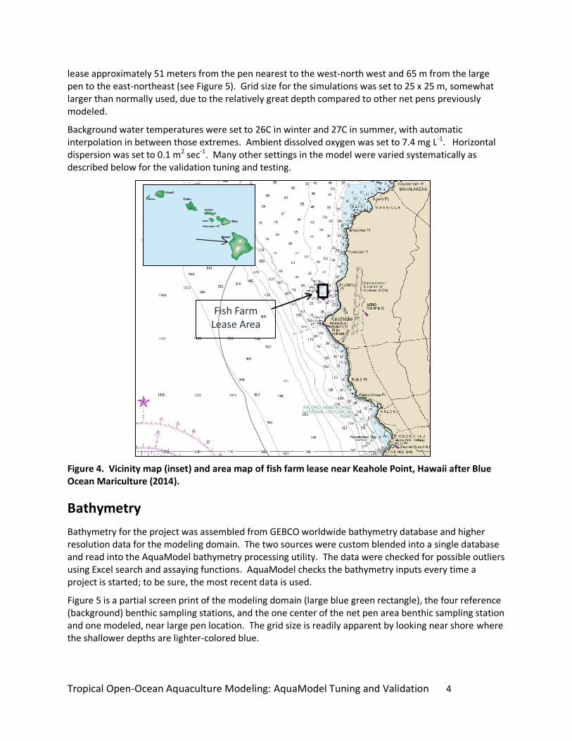
AquaModel was set up with a local shoreline, digitized from local charts and Google Earth. Bathymetry (Figure 4) was provided by Ken Riley, NOAA National Ocean Survey with the highest available resolution.
A rectangular modeling array of 1.3 km (north/south) and 1.0 km (east/west) was established around the center of the net pen lease area in AquaModel. Data capture cells were established for the four or more reference-benthic sampling stations and the one net pen station located within the center of the
Tropical Open-Ocean Aquaculture Modeling: AquaModel Tuning and Validation 4
Fish Farm Lease Area
lease approximately 51 meters from the pen nearest to the west-north west and 65 m from the large pen to the east-northeast (see Figure 5). Grid size for the simulations was set to 25 x 25 m, somewhat larger than normally used, due to the relatively great depth compared to other net pens previously modeled.
Background water temperatures were set to 26C in winter and 27C in summer, with automatic interpolation in between those extremes. Ambient dissolved oxygen was set to 7.4 mg L-1. Horizontal dispersion was set to 0.1 m2 sec-1. Many other settings in the model were varied systematically as described below for the validation tuning and testing.
Figure 4. Vicinity map (inset) and area map of fish farm lease near Keahole Point, Hawaii after Blue Ocean Mariculture (2014).
Bathymetry
Bathymetry for the project was assembled from GEBCO worldwide bathymetry database and higher resolution data for the modeling domain. The two sources were custom blended into a single database and read into the AquaModel bathymetry processing utility. The data were checked for possible outliers using Excel search and assaying functions. AquaModel checks the bathymetry inputs every time a project is started; to be sure, the most recent data is used.
Figure 5 is a partial screen print of the modeling domain (large blue green rectangle), the four reference (background) benthic sampling stations, and the one center of the net pen area benthic sampling station and one modeled, near large pen location. The grid size is readily apparent by looking near shore where the shallower depths are lighter-colored blue.

Tropical Open-Ocean Aquaculture Modeling: AquaModel Tuning and Validation 5
Figure 5. Modeling domain (blue/green rectangle) and study locations cited in this report.
Current Meter Deployment
A Teledyne RDI 300 kHz Workhorse acoustic Doppler current profiler (ADCP) was installed in the middle of the lease area in about 64 meters (210 feet) depth on October 2, 2013. This location was not immediately next to any of the pens but between and slightly south of two of the pens, one small on the west and one larger one on the east. The current meter was recovered on December 3, 2013. The location of the current meter as recovered was 19.742822 and -156.061884. The unit was set to record (ensemble interval) every 20 minutes with 10 bins of 6 meters each.
After the two-month deployment, the ADCP was recovered by a diver attaching a line. Downloaded data were inspected for obvious outliers and missing data. Some missing data (<5% of the time periods) were noted, mostly nearest the bottom, apparently due to interferences from nearby anchor lines that occasionally came into view of the ADCP transducers. These missing periods were brief, usually just a few ensembles. AquaModel uses data from all available depths to track particulate settling matter, so the occasional loss of one depth measurement series does not represent a significant problem.

Tropical Open-Ocean Aquaculture Modeling: AquaModel Tuning and Validation 6
After inspection of the data in WinADCP software and Excel spreadsheets, the top two, near surface bins were judged inappropriate for use due to backscatter from the water-atmosphere interface and related factors such as wave turbulence. Removal of the top 7 to 10% of the bin measurements is common for bottom mounted ADCP measurements. The second bin from surface was also deleted due to large numbers of missing data and because it was irrelevant to the study as the pens were below it. The depth bin nearest the bottom was set at 8.2 meters vertical span and the remaining bins were 6 meters deep.
A feature of AquaModel was used to interpolate for missing data that involves using the known data before and after the observed missing data. These data were then entered into the program as text data and AquaModel converted them to binary data that is read rapidly each time the model project was started.
Field and Laboratory Methods
Field sampling near the study site has been conducted with a hand-pulled Ponar grab sampler and GPS used for positioning. Surficial (2cm deep) samples were collected by coring, placed in whirl pac bags and on ice, then frozen later that same day for analysis. Because of the coarse nature of the bottom, repetitive samples were collected until adequate volume of sample was available.
Laboratory analysis of sea bottom sediments for total organic carbon content was required for this study. Although total organic carbon is a routine procedure, it is the primary author’s experience that accuracy and precision of analysis varies considerably from one laboratory to the next. We decided also to perform an inter-laboratory comparison of sample splits, with sample splits (from the same grab and core) sent to the University of Hawaii Hilo to be compared with a commercial laboratory in Seattle.
One of the difficult issues with TOC analysis of sediments from tropical, blue-water open ocean areas (i.e., not lagoons, mangrove coastlines and riverine estuaries) involves the fact that the concentration of TOC is usually small but there is often a large amount of inorganic carbon that can interfere with TOC analysis. The inorganic carbonates are present due to feeding of some types of fish (e.g., parrot fish) on corals or by erosion from dead corals. Some types of lava are also rich in inorganic carbon including carbonatite. Unless this inorganic carbon is carefully removed by treatment with dilute acid before TOC analysis, results can be an order of magnitude or more inaccurate. Compounding this problem is the fact that there is not much guidance on how to do the acid pretreatments, except to do it slowly, with weak acids, and continue until the obvious fizzing of the carbonates ceases.
When this study was commenced, both laboratories were considered expert at the pretreatment methods but the University of Hawaii Hilo laboratory had the advantage of having processed many samples before, including prior years of samples from the Blue Ocean Mariculture project, and was familiar with the process involving high inorganic carbonate samples. Moreover, the Hilo laboratory used a state-of-the-art CHN analyzer with good detection limits. The analyzer uses automated combustion processes to break down substances into simple compounds that are then quantified by infrared spectroscopy. The Seattle laboratory used EPA method 9060 with a laboratory-specific detection limit of 0.01%. This method at this and many other laboratories yields a duplicate difference of around 5 to 10% or more, so the results are never highly precise.
When the results were compared, we observed a very large difference between the two laboratories, with the Seattle laboratory producing results that were readily apparent to be incorrect as there was a large range of results, and the mean TOC concentrations were unreasonably high for open-ocean, tropical seas (or coastal shelf in this case). It was discovered that the laboratory staff responsible for

Tropical Open-Ocean Aquaculture Modeling: AquaModel Tuning and Validation 7
testing had quit their position just prior to our samples arriving and that an inexperienced analyst had conducted the analysis. The laboratory did not charge for the service and we rejected the data as not useful but in the process learned that the local laboratory was very careful to remove inorganic carbonates from the samples.
Fish Physiology Submodel
AquaModel uses species-specific physiology models expressly developed for individual ecoregions. There are now 10 separate fish species submodels and for this project we developed a submodel for Seriola rivoliana (also known as KampachiTM, Kona Kampachi, Kahala, almaco jack and long-fin yellow tail, see Figure 6). This is a fish native to the Hawaiian Islands but not normally fished as wild fish consume food sources affected by a benthic dinoflagellate that can cause ciguatera toxicity. This submodel was prepared by our team with fish farm specific growth data provided by Blue Ocean Mariculture. Wild fish data is not typically used in our AquaModel growth models, as farmed fish growth dynamics are different from wild fish in most cases.
Figure 6. Photograph of Seriola rivoliana grown at the subject fish farm.
Photo provided by Blue Ocean Mariculture.
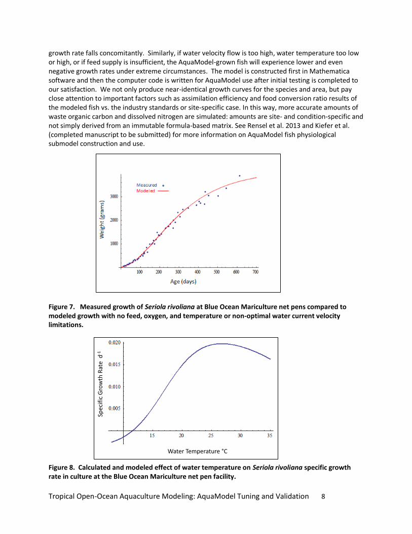
The S. rivoliana growth model was patterned around the actual growth performance of fish at the Blue Ocean Mariculture facility and their food conversion ratio and water temperatures encountered (Figures 7 and 8). AquaModel can be run with actual feed use inputs, but in this case they were not available and instead we utilized the optimum feed rate utility of AquaModel with an estimated feed loss of 3% of total feed used. In other validation studies we are finding that the optimum feed rate utility provides a good estimate of the feed use, and the actual loss rate of 3% is considered an industry standard at present. However, we considered alternative rates in this project as described below.
The actual growth of the fish in the model is not automatic or based on simple time sequences and feed charts, but based on a simulated environment and limiting factors that fish actually encounter. For example, if the fish are too crowded and dissolved oxygen declines below a threshold range the specific
Tropical Open-Ocean Aquaculture Modeling: AquaModel Tuning and Validation 8
Spec
ific
Gro
wth
Rat
e d
-1
Water Temperature °C
growth rate falls concomitantly. Similarly, if water velocity flow is too high, water temperature too low or high, or if feed supply is insufficient, the AquaModel-grown fish will experience lower and even negative growth rates under extreme circumstances. The model is constructed first in Mathematica software and then the computer code is written for AquaModel use after initial testing is completed to our satisfaction. We not only produce near-identical growth curves for the species and area, but pay close attention to important factors such as assimilation efficiency and food conversion ratio results of the modeled fish vs. the industry standards or site-specific case. In this way, more accurate amounts of waste organic carbon and dissolved nitrogen are simulated: amounts are site- and condition-specific and not simply derived from an immutable formula-based matrix. See Rensel et al. 2013 and Kiefer et al. (completed manuscript to be submitted) for more information on AquaModel fish physiological submodel construction and use. Figure 7. Measured growth of Seriola rivoliana at Blue Ocean Mariculture net pens compared to modeled growth with no feed, oxygen, and temperature or non-optimal water current velocity limitations.
Figure 8. Calculated and modeled effect of water temperature on Seriola rivoliana specific growth rate in culture at the Blue Ocean Mariculture net pen facility.

Tropical Open-Ocean Aquaculture Modeling: AquaModel Tuning and Validation 9
Conceptual Overview of Circulation and Benthic Submodels
AquaModel’s circulation routine is based on inputs from current meter measurements or output from 2D or 3D circulation models such as ROMS, DELFT and FVCOM as well as others. This powers water movement and rate of exchange among the grid cells in AquaModel for dissolved compounds and particles. However, the dissolved portion involves advection and turbulent mixing in the modelling array while the particulates are moved via a particle tracking routine that utilizes sinking rate factors and lateral movement and dispersion using a proprietary particle tracking routine unique to AquaModel. In this routine, the particles are moved with the currents, settle on the bottom when bottom velocity thresholds of flow are crossed and are resuspended at different thresholds described herein. This allows waste feed and fish feces to be transported independent of the model grids to the sea bottom where the particles remain or where water currents allow for resuspension and lateral transport. The organic carbon content of the particles is constantly being respired by benthic and epibenthic bacteria and organisms, including aerobic and anaerobic populations. The user enters via a graphical interface the number and size of cells within the array as well as its geolocation, orientation, and boundary conditions.
The benthic model describes the deposition, resuspension, transport and assimilation of particulate organic carbon beneath the cages as well as the surrounding waters. It also describes the growth and respiration of the benthic community that assimilates the deposited material. Benthic metabolism is assumed to be dominated by bacterial metabolism consisting of a variable mix of aerobic species and anaerobic species that compete for organic carbon. Growth of the aerobic assemblage is favoured when the diffusive flux of oxygen through the benthic boundary layer to the sediments meets the demand of the assemblage. This demand will vary with water temperature and the rate of organic deposition. The rate of supply of oxygen will vary with the gradient in oxygen concentration between the sediment surface and the suspended layer immediately above the sediments and bottom shear. If the rate of oxygen demand exceeds the rate of supply, the oxygen concentration in the upper layer of the sediments will drop below a threshold value that supports rapid metabolism of the aerobes and the metabolism of the anaerobic assemblage will now be favoured. The growth and respiration of the anaerobic assemblage is tracked by the respiration of sulphate and the production of hydrogen sulphide that diffuses from the sediments into the suspended water layer immediately above the sediments.
Unlike the other fish farm models which involve sediment chemistry, AquaModel has a working resuspension system that conserves the normal, steady-state concentration of organic carbon in reference areas remote from the fish farm effects. It also allows for elevated deposition and accumulation of TOC immediately beneath fish farms IF the TOC delivery rate exceeds the ability of the sediments to oxidize them. The model can be used to configure fish farms to achieve very little or no adverse sediment chemistry or biological effects if desired.
Importantly, our standard procedure is to adapt AquaModel to each ecoregion where it is applied. We do not assume or believe that the processes involved are identical in disparate ecoregions with varying sediment particle size distribution, infauna communities, ambient loading rates of natural sources of particulate organic carbon, etc. For example, in North and South America where salmon farms are located there are often very similar growing conditions and model settings, allowing us to more easily adapt and validate the model among such areas. Other components of AquaModel may have to be altered for different ecoregions, including the fish species physiology submodel, for example for Atlantic salmon (Salmo salar) that operates the same for the west coast of North and South America salmon farms. In this case the S. salar model was modified for growth factors for Eastern Canada due to

Tropical Open-Ocean Aquaculture Modeling: AquaModel Tuning and Validation 10
different patterns of growth that we found that were not solely accounted for by water temperature variables in the growth model.
Sensitivity Testing Background
AquaModel has been used for 14 years in a number of locations worldwide and a number of less formal efforts have been used in the past to calibrate the model including assessments using the equations of the model, interlinked but tested within Mathematica software to establish near-correct settings for specific projects within distinct ecoregions.
In 2013 we began more formal validation of the benthic component of the model including this project and several other pens located in two foreign countries. One of those efforts is nearly complete (Rensel et al. 2014) and by comparing and contrasting results and different site conditions, further insight into AquaModel performance with different settings became more apparent.
In the process of using a visual-oriented output model like AquaModel, after several years of use we had already collected some sensitivity testing data and had a good feel for the primary factors controlling the outcome of the model in different categories of oceanographic conditions. This was based on less formal validation efforts and available literature. Few aquaculture models have been validated and those that claim validation have done so using surrogate measures that do not address waste organic matter distribution and fate. Creation of an aquaculture model is just step one in a long series of steps to test, tune, reconfigure, re-tune and arrive at an acceptable product. No other fish aquaculture models have ever been subjected to the years of testing, tuning, alteration, retesting and tuning that AquaModel has been through.
At least one other model claims successful validation, but in all cases we could find, it was not a holistic validation but rather a piecemeal validation. By holistic we mean that the model inputs resulted in a primary effect (in our case, benthic organic matter flux) and the model was tested for accuracy of matching observed measurement. We did not use, surrogate measures, such as spatial distribution of glass beads or an indirect measure of organic loading such as sediment sulfide concentration or collection of wastes in sediment cups. These d9nnot allow for particle resuspension, transport and food web assimilation if water currents are sufficiently strong.
This section describes our empirical and relatively uncomplicated approach to sensitivity testing. But some background is useful too, as follows.
First, “sensitivity analysis may be defined as study of uncertainty of output of a numerical model or system that can be can be assigned to various sources of uncertainty from model inputs” (paraphrased from several different literature citations). Such analysis is part of the model calibration process defined as a process “to achieve a desired degree of correspondence between the model output and actual observations of the environmental system that the model is intended to represent” (EPA 2002).
From Pannell (1997): The goals associated with sensitivity testing include, but are not limited to:
Testing the robustness of the results of a model or system in the presence of uncertainty.
Increased understanding of the relationships between input and output variables in a system or model.
Uncertainty reduction: identifying model inputs that cause significant uncertainty in the output and therefore should be the focus of attention if the robustness is to be increased (perhaps by further research).

Tropical Open-Ocean Aquaculture Modeling: AquaModel Tuning and Validation 11
Searching for errors in the model (by encountering unexpected relationships between inputs and outputs).
Model simplification – fixing model inputs that have no effect on the output, or identifying and removing redundant parts of the model structure.
Enhancing communication from modelers to decision makers (e.g. by making recommendations more credible, understandable, compelling or persuasive).
Finding regions in the space of input factors for which the model output is either maximum or minimum or meets some optimum criterion.
To some degree, all of the above goals except the final one are applicable to the present study.
Sensitivity Testing Methods
There is a profuse, conflicting and often confusing literature regarding aquatic model sensitivity testing. No one accepted method is available that must be used or that is considered best used for the present circumstance. Most of the techniques we reviewed were cryptic and complex with only modestly meaningful documentation at best resulting in unconvincing analysis overall.
Categorically, sensitivity techniques could be considered as “one-factor-at-a-time” variable analysis or “multiple-interacting factor” variable analysis or some mixture of the two. The latter can become much more complex because the number of factors considered rapidly expands the number of trials required on a factorial analysis basis (e.g., 5 factorial = 120 trials, 6 factorial = 720 trials, etc. rapidly into the millions of trials). There are methods to address this problem such as the use of statistical Monte Carlo computational algorithms, but such approaches were deemed unsuitable in our case. These algorithms require that inputs be drawn from random sampling within a range of possible inputs. This was neither possible nor desirable in our situation where we have specific knowledge about optimum estimates for several of the parameters of interest. The following describes our approach and justification.
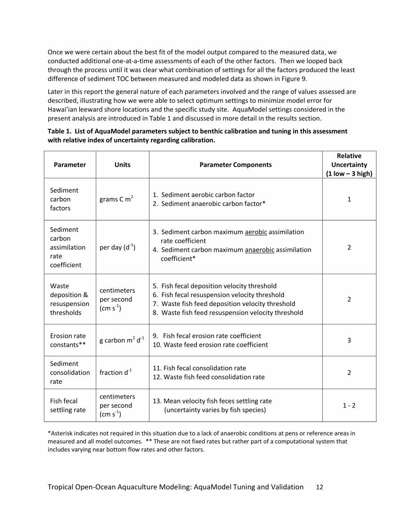
The five major factors considered for this benthic submodel validation are presented in Table 1 along with the sub-factors. This table ranks the relatively uncertainty of optimum settings for each parameter, based on our experience, knowledge and literature citations.
Our testing strategy was to perform a hierarchical approach starting with what we knew without doubt to be the most influential parameter in AquaModel’s benthic submodel (see Figure 9). The process involved sequential steps including:
1) Determining the modeling outcomes for variation of most important single or multiple combined parameter settings to find an interim best fit value (but not always initially obtaining a close fit);
2) Combining the best initial fits for all other parameters with those of number 1 above and varying all of them concurrently within a reasonable range of settings to estimate best fit for one time period of the fish culture;
3) Determining if any of the factors had strong interaction effects of other factors,
4) Combining and contrasting the best-fit observations for separate endpoint times to estimate the cumulative time-period best-fit settings while focusing on factors with interactions.
In the Blue Ocean Mariculture validation study, we relied on estimated steady state concentration of sediment TOC in reference and near pen areas, so number three above was not necessary.
Tropical Open-Ocean Aquaculture Modeling: AquaModel Tuning and Validation 12
Once we were certain about the best fit of the model output compared to the measured data, we conducted additional one-at-a-time assessments of each of the other factors. Then we looped back through the process until it was clear what combination of settings for all the factors produced the least difference of sediment TOC between measured and modeled data as shown in Figure 9.
Later in this report the general nature of each parameters involved and the range of values assessed are described, illustrating how we were able to select optimum settings to minimize model error for Hawai’ian leeward shore locations and the specific study site. AquaModel settings considered in the present analysis are introduced in Table 1 and discussed in more detail in the results section.
Table 1. List of AquaModel parameters subject to benthic calibration and tuning in this assessment with relative index of uncertainty regarding calibration.
Parameter Units Parameter Components Relative
Uncertainty (1 low – 3 high)
Sediment carbon factors
grams C m2 1. Sediment aerobic carbon factor 2. Sediment anaerobic carbon factor*
1
Sediment carbon assimilation rate coefficient
per day (d-1)
3. Sediment carbon maximum aerobic assimilation rate coefficient 4. Sediment carbon maximum anaerobic assimilation coefficient*
2
Waste deposition & resuspension thresholds
centimeters per second (cm s-1)
5. Fish fecal deposition velocity threshold 6. Fish fecal resuspension velocity threshold 7. Waste fish feed deposition velocity threshold 8. Waste fish feed resuspension velocity threshold
2
Erosion rate constants**
g carbon m2 d-1 9. Fish fecal erosion rate coefficient 10. Waste feed erosion rate coefficient
3
Sediment consolidation rate
fraction d-1 11. Fish fecal consolidation rate 12. Waste fish feed consolidation rate
2
Fish fecal settling rate
centimeters per second (cm s-1)
13. Mean velocity fish feces settling rate (uncertainty varies by fish species)
1 - 2
*Asterisk indicates not required in this situation due to a lack of anaerobic conditions at pens or reference areas in measured and all model outcomes. ** These are not fixed rates but rather part of a computational system that includes varying near bottom flow rates and other factors.

Tropical Open-Ocean Aquaculture Modeling: AquaModel Tuning and Validation 13
1: Preliminarily set reference
(background) area sediment total
organic carbon concentrations to
measured values in region:
If necessary for higher precision, iterate
with combined aerobic and anaerobic
carbon factors and maximum
assimilation rate coefficients*
2: Establish net-pen area total organic
carbon concentrations to match average
measured values at fish production steady
state or time series values:
Iterate with anaerobic carbon factor and
maximum assimilation rate settings only for
best fit. Background TOC will remain
unaffected and at steady state if current
velocity is approximately correct
4: Vary fish fecal and waste feed
deposition and resuspension
threshold flow velocity around
prior AquaModel & literature
values, as these are somewhat well
known.
One at a time, then as a group of all
four concurrently
Skip Step 2 for moderate-size farms in fast or
deep waters and if preliminary runs or field data
show no evidence of surficial sediment hypoxia
and related effects under or near pens
5: Vary erosion rate coefficient for
waste feed and fish fecal
separately, then together.
Use guidance from other similar
ecoregions for starting point
AquaModel Regional Benthic Effects
Tuning & Validation Protocol*
6: Set Consolidation Rate low (e.g., 0.1) for
oligotrophic/fast flowing sites and high
(e.g.,0.7) for eutrophic/slow flowing sites.
Iterate to maintain observed background TOC
concentrations and balance with average net
pen TOC observed
Return to Step 3 to fine tune TOC
aerobic and Rate k factors if needed to
achieve improved accuracy. Process is
completed when fit is close and individual
station variability from observed values
is minimal.
3: Assess all other factors one-at-a- time
and determine if trend exists over a range
of reasonable values. Identify factors with
strong interactions for additional testing.
In following steps 4-6, use standard
recommendations for the few parameters that
exhibit no trend effects over a broad range of
typical values.
* Use of settings from similar ecoregions can be used
to expedite this process and greatly reduce time and
number of iterative steps.
Most importantly: This validation protocol is not
required for routine AquaModel use by end users.
AquaModel staff provides the correct or approximately
correct values in most circumstances.
Figure 9. Flow chart for calibrating and tuning AquaModel to individual ecoregions. Process is performed by AquaModel (SSA) staff, not end users. Blue arrows main = main path, green arrows = alterative paths.
Tropical Open-Ocean Aquaculture Modeling: AquaModel Tuning and Validation 14
We began the validation and tuning process with sediment carbon factors and maximum assimilation rate estimates for aerobic and anaerobic conditions. Sediment organic carbon is the principal endpoint of AquaModel’s benthic effects architecture and all of the factors considered involve this end point, but the relative influence of each factor varies considerably. These are the primary factors in the sediment model but of course other factors in the model greatly influence them such as the total biomass of cultured fish, the percent loss rate of fish feed, the fish feed composition, site depth, current velocities and direction, etc. Most of these factors can be estimated with reasonable accuracy but we acknowledge that some are difficult to prove such as the 3% loss rate of fish feed generally considered by the industry as the norm using current best management practices. Industry representatives and scientists often make the salient point that fish stock biomass assessment is relatively accurate and that if the loss rate was much larger, the economics of fish culture would be marginal or prohibitive.
Results: Measured Study Site Conditions
Current meter results
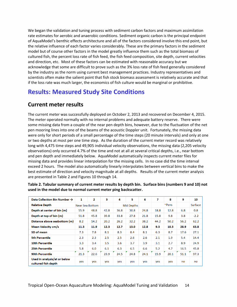
The current meter was successfully deployed on October 2, 2013 and recovered on December 4, 2015. The meter operated normally with no internal problems and adequate battery reserve. There were some missing data from a couple of the near pen depth bins, however, due to the fluctuation of the net pen mooring lines into one of the beams of the acoustic Doppler unit. Fortunately, the missing data were only for short periods of a small percentage of the time steps (20 minute intervals) and only at one or two depths at most per one time step. As the duration of the current meter record was relatively long with 4,475 time steps and 49,905 individual velocity observations, the missing data (2,205 velocity observations) only occurred 4.7% of the time and not at all at several critical depths, i.e., near bottom and pen depth and immediately below. AquaModel automatically inspects current meter files for missing data and provides linear interpolation for the missing cells. In no case did the time interval exceed 2 hours. The model also automatically linearly interpolates between vertical bins to make the best estimate of direction and velocity magnitude at all depths. Results of the current meter analysis are presented in Table 2 and Figures 10 through 14.
Table 2. Tabular summary of current meter results by depth bin. Surface bins (numbers 9 and 10) not used in the model due to normal current meter ping backscatter.
Tropical Open-Ocean Aquaculture Modeling: AquaModel Tuning and Validation 15
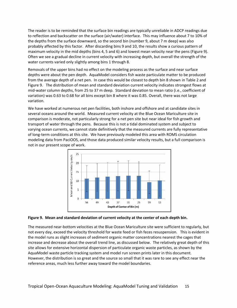
The reader is to be reminded that the surface bin readings are typically unreliable in ADCP readings due to reflection and backscatter on the surface (air/water) interface. This may influence about 7 to 10% of the depths from the surface downward, so the second bin (number 9, about 7 m deep) was also probably affected by this factor. After discarding bins 9 and 10, the results show a curious pattern of maximum velocity in the mid depths (bins 4, 5 and 6) and lowest mean velocity near the pens (Figure 9). Often we see a gradual decline in current velocity with increasing depth, but overall the strength of the water currents varied only slightly among bins 1 through 8.
Removals of the upper bins had no effect on the modeling process as the surface and near surface depths were about the pen depth. AquaModel considers fish waste particulate matter to be produced from the average depth of a net pen. In case this would be closest to depth bin 8 shown in Table 2 and Figure 9. The distribution of mean and standard deviation current velocity indicates strongest flows at mid-water column depths, from 25 to 37 m deep. Standard deviation to mean ratio (i.e., coefficient of variation) was 0.63 to 0.68 for all bins except bin 8 where it was 0.85. Overall, there was not large variation.
We have worked at numerous net pen facilities, both inshore and offshore and at candidate sites in several oceans around the world. Measured current velocity at the Blue Ocean Mariculture site in comparison is moderate, not particularly strong for a net pen site but near ideal for fish growth and transport of water through the pens. Because this is not a tidal dominated system and subject to varying ocean currents, we cannot state definitively that the measured currents are fully representative of long-term conditions at this site. We have previously modeled this area with ROMS circulation modeling data from PaciOOS, and those data produced similar velocity results, but a full comparison is not in our present scope of work.
Figure 9. Mean and standard deviation of current velocity at the center of each depth bin.
The measured near-bottom velocities at the Blue Ocean Mariculture site were sufficient to regularly, but not every day, exceed the velocity threshold for waste feed or fish feces resuspension. This is evident in the model runs as slight increases of sediment organic matter concentrations nearest the cages that increase and decrease about the overall trend line, as discussed below. The relatively great depth of this site allows for extensive horizontal dispersion of particulate organic waste particles, as shown by the AquaModel waste particle tracking system and model run screen prints later in this document. However, the distribution is so great and the source so small that it was rare to see any effect near the reference areas, much less further away toward the model boundaries.

Tropical Open-Ocean Aquaculture Modeling: AquaModel Tuning and Validation 16
Figure 10. Velocity plot for the entire current meter deployment period (across the image, above), an excerpted section from ensemble 1000 to 2000 (about 25 to 45% through the entire deployment) and a plot of velocity magnitude for bins 5 and 6, (mid depth, the line plot at the bottom).
Figure 11 includes the near-surface depth bins that were discarded from the analysis due to normal backscatter and wave turbulence. Note periodic occurrence of slightly faster currents indicated by the light blue-to-blue-green bands, with the exception of the middle of the deployment near ensemble date 2250. Black areas represent period when anchor lines blocked one or more of the current meter beams.
Tropical Open-Ocean Aquaculture Modeling: AquaModel Tuning and Validation 17
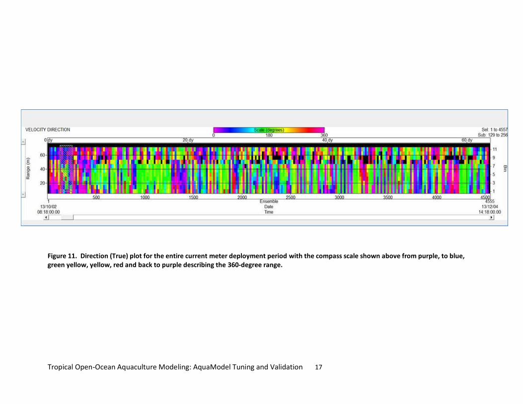
Figure 11. Direction (True) plot for the entire current meter deployment period with the compass scale shown above from purple, to blue, green yellow, yellow, red and back to purple describing the 360-degree range.

Tropical Open-Ocean Aquaculture Modeling: AquaModel Tuning and Validation 18
Figure 12. AquaModel current vector rose for one and two month’s elapsed time at net pen depth.
Figure 13. AquaModel current vector rose for one and two month’s elapsed time near sea bottom.
Tropical Open-Ocean Aquaculture Modeling: AquaModel Tuning and Validation 19
Far Field Circulation
In order to understand circulation at a fish farm site, it is desirable to have a broader view of current flows than just at one current meter site. Having more than one current meter site yields information, but no models are available that are capable of integrating two or more current meter records. Far field models are useful to describe circulation patterns over large areas, but often for small areas of fish farm modeling, the resolution of such models is poor for benthic effects forecasting. We examined the northern leeward coast of the Island of Hawaii previously (O’Brien et al. 2011) using far field model data from the Pacific Islands Ocean Observation System (PacIOOS) to power AquaModel. The system performed well for large area issues, but for relatively small modeling grids such as the one used in this study, the resolution of the PacIOOS model is insufficient. It is possible to increase resolution of a model by doing so in discrete, nested areas, but it takes sufficient funds and time. As an alternative to far field models, the primary author attempted to collect far field information using surface drifters released near the fish farm on eastern and western sides and at different depths as described below. Surface drifters and window shade drogues were shipped to the project site, assembled and deployed beginning on the morning of October 4, 2013. The reconstructed drogues were deployed as pairs, sequentially within a few minutes of other, both inshore and offshore of the fish farm lease area along a transect line perpendicular to shore. The drogues nearest shore moved tangentially toward shore and the southeast. When nearing shallow water they began moving parallel to the shore to the south and following a relatively constant depth profile. Drogues released offshore of the farm site moved in a consistently northerly direction. Early in the day, the support vessel began to have engine problems and due to a lack of other available vessels, no further drogue releases were possible. These data, along with anecdotal evidence from those working at or familiar with the site, suggest that the predominant offshore flow at the time of sampling was from the south to the north but that nearer shore there may have been a backeddy (gyre) flowing in the opposite direction to the south. Although the fish farm is in open ocean conditions, it is physically located relatively near shore. Eddies are common downstream of prominent points of land in the sea, and will disappear when the offshore flow reverses or alters direction. We emphasize that the current meter results appear to be representative of the net pen area and that the drogue observations were based on initial locations relatively far to the west and east of the net pens.
Sediment Testing Results
Routine benthic grab sampling of five stations near the project site have been conducted annually since 2007. The parameters of particular interest to modeling are sediment total organic carbon (TOC) and to a lesser extent, sediment grain size analysis. In this area the sediment TOC sampling results have been without exception very low compared to inshore waters where fish and shellfish aquaculture is mostly practiced in the United States, as well as in major fish-aquaculture producing countries such as Canada and Chile. TOC is inversely correlated with percent silt and clay, and as an example at project site in 2013 sediment samples averaged only 0.5% fines.
In comparison, salmon farming sites in North and South America have background (unaffected reference areas or pre-existing ) TOC concentrations that generally range from ~0.25% dry weight (for areas with < 2 to 20% silt and clay) to ~2.5% for areas with > 70% silt and clay. The AquaModel team also works in other countries with TOC concentrations of > 6% in reference locations near fish farms with >80% fines, and therefore the conditions at the project site location and similar regions of Hawaii are indeed on the
Tropical Open-Ocean Aquaculture Modeling: AquaModel Tuning and Validation 20
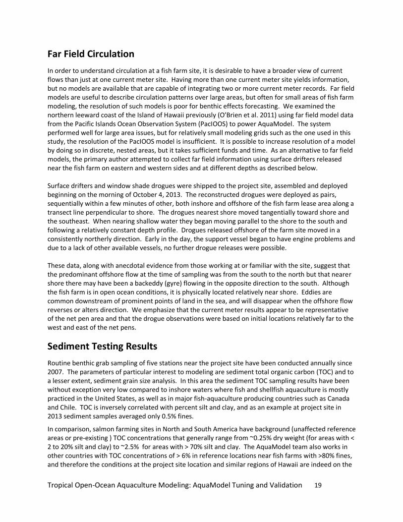
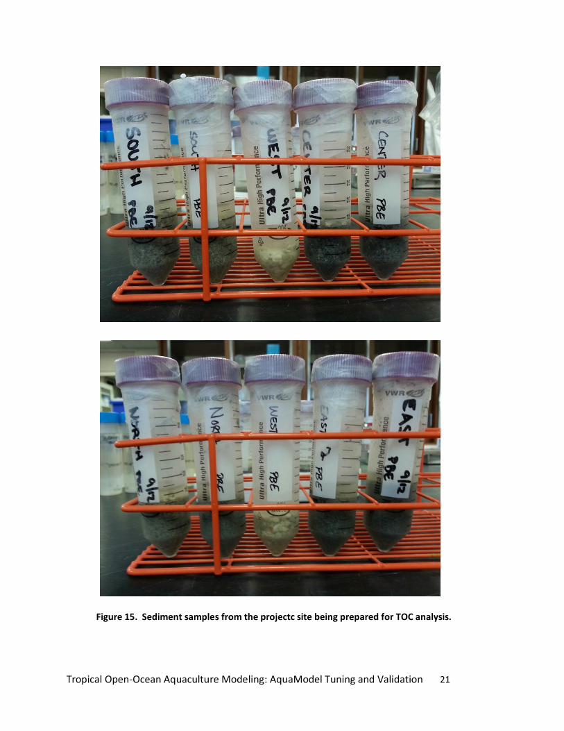
very low end of the scale in terms of sediment organic enrichment. Figure 15 illustrates a dried, ready for laboratory analysis view of one of the 2013 samples taken at the project site. Figure 16 is of the samples in the laboratory before drying showing different degrees of darkness and grain size.
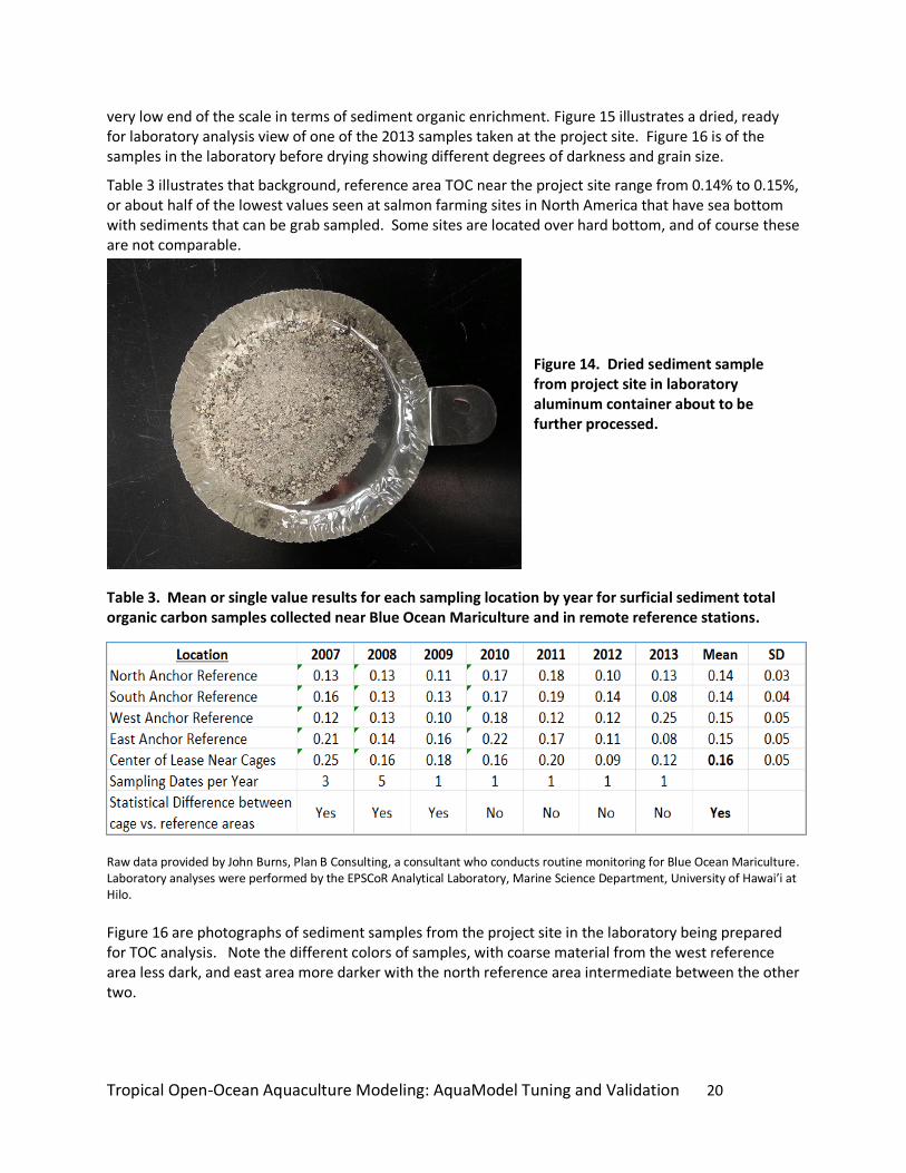
Table 3 illustrates that background, reference area TOC near the project site range from 0.14% to 0.15%, or about half of the lowest values seen at salmon farming sites in North America that have sea bottom with sediments that can be grab sampled. Some sites are located over hard bottom, and of course these are not comparable.
Figure 14. Dried sediment sample from project site in laboratory aluminum container about to be further processed.
Table 3. Mean or single value results for each sampling location by year for surficial sediment total organic carbon samples collected near Blue Ocean Mariculture and in remote reference stations.
Raw data provided by John Burns, Plan B Consulting, a consultant who conducts routine monitoring for Blue Ocean Mariculture. Laboratory analyses were performed by the EPSCoR Analytical Laboratory, Marine Science Department, University of Hawai’i at Hilo.
Figure 16 are photographs of sediment samples from the project site in the laboratory being prepared for TOC analysis. Note the different colors of samples, with coarse material from the west reference area less dark, and east area more darker with the north reference area intermediate between the other two.
Tropical Open-Ocean Aquaculture Modeling: AquaModel Tuning and Validation 21
Figure 15. Sediment samples from the projectc site being prepared for TOC analysis.

Tropical Open-Ocean Aquaculture Modeling: AquaModel Tuning and Validation 22
Statistical testing of field sampling results
In order to evaluate the minor differences of sediment total organic carbon results among sampling locations, we divided the results into reference stations (N = 4) and treatment station (N =1, i.e., the center of the lease area near the center of the cages). No actual within-years, same day replicate samples were collected, although in some years single samples were collected on different days. Annual mean sediment TOC was calculated from all these data as shown in Table 3. Although this is not as ideal as replicate samples for each time period most commonly used to conduct parametric statistical evaluations, these were the available data.
Next, a one sample Student’s t tests was conducted to evaluate the data in Table 3. This test is often used to test of whether the mean of a population has a value specified in a null hypothesis and widely used for regulatory testing. The one-sample t-test is best used when you need to know if the sample data originates from a particular population but we do not have full population information available to us. In this case, we do not have full information about the net pen location except for one location. The appropriate hypothesis tests whether the average of our sample from the reference areas comes from a population with a known mean or some other different population.
Next, the question was posed, what is the most reasonable reference area data to use? In net pen monitoring, reference areas are usually selected as being distant from the net pens, and having similar depth and sediment grain-size distribution. In this case, this means that the north and south reference locations were most suitable, as they were about the same depth compared to the center of the net pen area. Long-term sediment TOC results for these stations both averaged 0.14% with similar standard deviations of 0.03 and 0.04%.
The one sample t test was then applied to the annual data from the net pen location compared to the estimated reference location value of 0.14% TOC. This resulted in a significant statistical difference (p =0.035, df =6) between the reference value and the measured data for the net pen area. Inspection and plotting of the data indicated that the differences were mostly attributable to the period 2007-2009 when the farm was not owned by Blue Ocean Mariculture.
It is possible to conduct other types of tests with these data to indicate that there is no statistical difference among stations sampled. However, we know from monitoring data and modeling of numerous other locations worldwide that the highest probability of increased TOC is immediately beneath or adjacent to net pen locations, particularly when current vector patterns are partitioned somewhat evenly into opposite directions such as they were in the present study.
Overall, sediment TOC concentrations were very low at both treatment and reference sampling sites. Statistical differences between these location categories occurred but were mostly attributable to earlier years in the time series. Parametric statistical tests are easily skewed by a lack of replicates and small sample sizes, but by pooling the available observations, the latter is overcome. We can conclude that there is a hint of a difference between sediment TOC measured at the reference areas and the center of the lease area where grab samples are collected. While the pen area benthic sampling location is centered well among three cages, as is seen later in this report, the model predicts slightly higher TOC concentrations in most directions around that single point as waste feed sink relatively rapidly compared to fish feces.
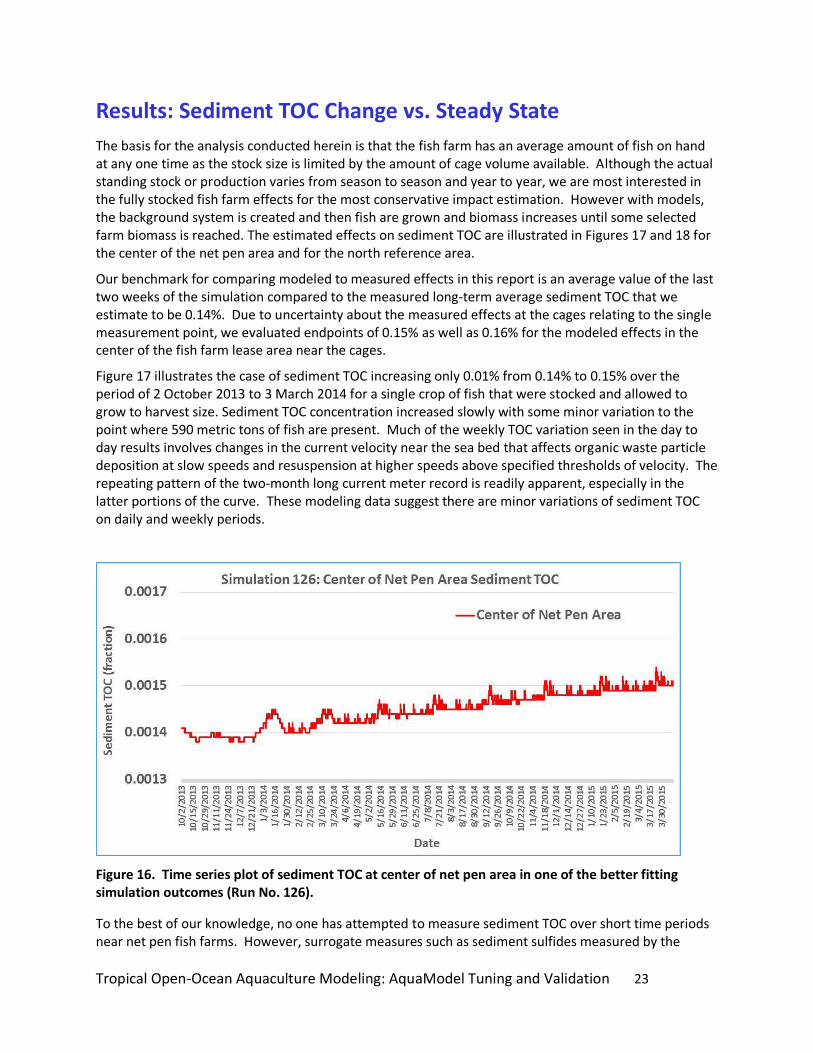
Tropical Open-Ocean Aquaculture Modeling: AquaModel Tuning and Validation 23
Results: Sediment TOC Change vs. Steady State
The basis for the analysis conducted herein is that the fish farm has an average amount of fish on hand at any one time as the stock size is limited by the amount of cage volume available. Although the actual standing stock or production varies from season to season and year to year, we are most interested in the fully stocked fish farm effects for the most conservative impact estimation. However with models, the background system is created and then fish are grown and biomass increases until some selected farm biomass is reached. The estimated effects on sediment TOC are illustrated in Figures 17 and 18 for the center of the net pen area and for the north reference area.
Our benchmark for comparing modeled to measured effects in this report is an average value of the last two weeks of the simulation compared to the measured long-term average sediment TOC that we estimate to be 0.14%. Due to uncertainty about the measured effects at the cages relating to the single measurement point, we evaluated endpoints of 0.15% as well as 0.16% for the modeled effects in the center of the fish farm lease area near the cages.
Figure 17 illustrates the case of sediment TOC increasing only 0.01% from 0.14% to 0.15% over the period of 2 October 2013 to 3 March 2014 for a single crop of fish that were stocked and allowed to grow to harvest size. Sediment TOC concentration increased slowly with some minor variation to the point where 590 metric tons of fish are present. Much of the weekly TOC variation seen in the day to day results involves changes in the current velocity near the sea bed that affects organic waste particle deposition at slow speeds and resuspension at higher speeds above specified thresholds of velocity. The repeating pattern of the two-month long current meter record is readily apparent, especially in the latter portions of the curve. These modeling data suggest there are minor variations of sediment TOC on daily and weekly periods.
Figure 16. Time series plot of sediment TOC at center of net pen area in one of the better fitting simulation outcomes (Run No. 126).
To the best of our knowledge, no one has attempted to measure sediment TOC over short time periods near net pen fish farms. However, surrogate measures such as sediment sulfides measured by the

Tropical Open-Ocean Aquaculture Modeling: AquaModel Tuning and Validation 24
probe method in Eastern Canada have shown significant weekly variation (e.g., DFO 2012). Variation of water currents can explain much of this variation, with slow currents resulting in more sediment TOC accumulation and faster currents helping resuspend and relocate organic wastes. Moreover, Fickian diffusion of oxygen into the surficial layers of sediment is expedited by faster flowing bottom layers of water as the flux rate of oxygen is embellished. AquaModel’s benthic model is designed to allow for simulation of this effect. Variation of sediment TOC at the background area (Figure 18) shows that AquaModel is close to but not achieving 100% steady state with a slow accretion of TOC apparent, but at concentrations not detectable in field measurements. Yet the variation observed is far less than what is measurable in the field, just a few ten thousandths of the TOC fraction (or thousandths of percent TOC). We have found in this study that it is possible to adjust input settings to eliminate even such minor variation.
Figure 17. Time series plot of sediment TOC at the north reference area in one of the better fitting simulation outcomes (Run No. 126).
Tropical Open-Ocean Aquaculture Modeling: AquaModel Tuning and Validation 25
Results: Modeled versus Observed Sediment Effect Analysis A large number of initial model runs were completed where we conducted basic evaluation of particle tracking under set conditions and adjusted the physical processes in the model to achieve a finely tuned outcome. We also evaluated outcomes for possible model errors and inefficiencies on other accounts as described in the companion report to this one (Rensel et al. 2015b). Many small bugs and a few major bugs were discovered, studied, fixed and additional runs completed to be sure the problems were not recurring. This happened several times and each time all of the prior model runs considered important had to be re-run and reanalyzed with regard to the results. After several months of this we were able to conduct several hundred simulations, each requiring about 7 hours, to create a database to work with for this validation study. From experience and additional one-at-a-time testing, we determined that the following three factors were key parameters in the model. Shifting these parameters over a possible range of settings had a major effect on the intensity of sediment TOC effect.
Sediment Carbon Parameters
Overview
AquaModel uses a simple model of sediment diagenesis that involves both aerobic and anaerobic populations of organisms in the surficial, 2cm thick, uppermost layer of the sea bottom. Both aerobic and anaerobic organisms compete for the organic carbon wastes that fall to the seafloor or lake/river bottoms. As the rate of carbon delivery to the sea bottom increases, the concentration of interstitial dissolved oxygen declines in these sediments due to respiration of the benthic fauna. If the rate of enrichment continues, gradually the aerobic organisms are less able to compete in the hypoxic conditions. They then give way to the anaerobic organisms as the sediments become hypoxic or even anoxic in extreme cases. One of the principal purposes of AquaModel is to facilitate design of fish farms to avoid sediments hypoxia through site-specific configuration of the pen locations and sizes.
The organic carbon processing in AquaModel is based in part upon the well-known “G model” of Westrich and Bernier (1984) with some alterations we included to update the processes. In addition to oxygen supply, water temperature is a major controller of the sediment carbon assimilation and respiration rate processes but the actual rates of organic carbon processing are not readily available in the literature. Some data on oxygen respiration is available, but only in a few situations and not often related to sediment carbon processes. Sediment diagenesis can be an extremely complex process to describe or model, as the molecules of organic matter are readily available to react with oxidants that are electron receptors including respiration with oxygen and reduction with sequentially important nitrate, manganese, iron, and sulfate molecules (Stumm and Morgan 1995, Emerson and Hedges 2008). Oxygen is involved in the aerobic process near the sediment-water interface and the other oxidants may occur via anaerobic processes with increasing depth in a specific order in the sediments.
AquaModel simplifies the complex processes by considering only the ~ 2 cm deep surficial layer of the sediments, not the much deeper layers where organic carbon reduction occurs. This simplification is justified on several accounts including the fact that:
“In (oceanic) near-shore environments, where there is sufficient organic matter flux to the sediments to activate sulfate reduction and deplete sulfate in pore waters, zones of oxygen,

Tropical Open-Ocean Aquaculture Modeling: AquaModel Tuning and Validation 26
nitrate, and Mn(IV) reduction are very thin or obscured by benthic animal irrigation and bioturbation”\1.
AquaModel does not attempt to model environments such as shallow coastal mangrove swamps or coastal wetlands and some estuaries where the complex sediment diagenesis processes may occur as these are inappropriate locations for large-scale commercial net pens.
Moreover, particulate organic carbon from fish farms is generally considered highly labile (available for bacterial and other benthic consumers) versus refractive organic carbon sources, for example terrestrial plant matter such as tree bark. This fact is validated by the findings of numerous sediment recovery studies after cessation of net pen operation. Refractive organic carbon will take decades to decay (e.g., tree bark in commercial log rafting and dumping areas) but recovery from net pen sedimentation when it is extreme ranges from months for fast flowing waters to a few years at most for shallow, isolated areas with slow water circulation.
Process Description
Following a process flow chart (Figure 9), a stepwise process is used to determine suitable carbon factors, maximum carbon assimilation rates and other settings. As noted above, there are two types of factors for both aerobic and anaerobic carbon processing described below: 1) the carbon factor and 2) the sediment maximum assimilation rate coefficient.
The carbon factor is the background TOC concentration found in the subject area or region. This will vary somewhat, but often net pens are sited in similar depths and distances offshore that have similar sediment grain size distributions and organic carbon content. In lieu of TOC data, sediment total volatile solids (TVS) data may be used as a surrogate calibration measurement, particularly if a local conversion factor is available. Values we have empirically measured range from ~0.4 to 0.6 of TVS but in some eutrophic tropical conditions, these ratios may not apply. Fish farming over naturally or previously enriched sediments is not considered a sustainable practice, but it does occur in some regions including Southeast Asia.
The sediment maximum assimilation rate coefficient is a limiting function for the growth rate of sediment bacteria, both aerobic and anaerobic, that process much of the organic carbon arriving upon the sea bottom. The units of this setting are growth rate (doubling) per day expressed as d-1.
We have found it advantageous to establish the correct sediment aerobic factor as the first step. This is a simple process and is aided greatly by knowing the range of background TOC concentrations in the subject area or region. Sediment TOC is often fairly static in many sheltered, subtidal coastal environments as shown by decadal long studies once more common than now (Lie and Evans 1969). Concurrently, sediment TOC can remain within small ranges over even longer periods as shown in early Puget Sound Studies. However, major storms surges in some locations in shallow waters have been known to produce dramatic changes such as in Toothacre Cove in coastal Maine (Findlay and Watling 1997).
This first step is best performed without any fish in the virtual AquaModel pens, focusing on the aerobic factor to match the steady state background TOC concentrations at measured values. AquaModel has a 1 Here “inshore” means all marine waters of the continental or island shelves. Aquaculturists use different and vaguely-defined terms such as “open ocean” or “offshore” but with few exceptions these are restricted to continental (neritic) shelf areas and not the bulk of the oceans that are often over deeper (oceanic) waters except for some of the polar seas. Oceanographers use both physical and biological conditions to classify subdivisions of the oceans.
Tropical Open-Ocean Aquaculture Modeling: AquaModel Tuning and Validation 27
special process that allows users to attain a steady state condition within the normally occurring range of current flows that is beyond the scope of this report. Other models have had difficulty with establishing or maintaining a steady state background TOC, unless their resuspension modeling is turned off, a process that is necessary to make correct estimates in high capacity net pen sites. In such cases the sediment TOC is washed out of their modeling arrays when the current velocity increases (e.g., Chamberlain and Stucchi 2007 who used Depomod software).
The next step in adapting AquaModel to a new ecoregion is to modify the sediment anaerobic carbon factor until the predicted below or near pen sediment TOC reaches the mean value for the same locations in a data set from a representative farm in the region.
In our process, initially the same carbon factor values are assigned to the aerobic and anaerobic factors as an approximation. The literature generally indicates that rates of carbon flux in marine sediments are similar for both aerobic and anaerobic sediment conditions. However, mineralization of dissolved organic molecules may be less efficient under anaerobic (anoxic) conditions as proposed by Hansen and Blackburn (1991). Not all sediment organic carbon is equally labile, as discussed in our other reports following the work of Westrich and Berner (1984) on their seminal studies with the G model. The concept is that the rate of organic carbon respiration will depend upon composition of the particulate organic material: labile compounds will be respired at rates faster than refractive compounds. Each class of compound, labile or refractive, will be respired according to a first order reaction in which the rate of loss is a function of the product of the concentration of the compound and its rate constant. Thus the loss of particulate wastes by respiration is described as the sum of the respiration rates for each of the compounds.
Tlusty et al. (2000) demonstrated that fish fecal matter had a very high solubility potential, loosing approximately 50% of its organic matter in 12 day exposures to water flow. Besides solubility, bacterial use of the material is likely to be rapid. Fish feces are thus “non-refractive” forms of carbon, unlike carbon more tightly locked up in refractive forms such as tree trunks or bark or carbonate carbon such as shell. The most refractive organic carbon decays an order of magnitude more than the fastest types. Subsequent models of sediment respiration after Westrich and Berner (1984) demonstrated that below 2 cm sediment depth, other electron receptors become more important in the decomposition process and that rates decrease markedly (see review by Bianchi 2006).
AquaModel is structured to recognize that aerobic and anaerobic bacteria occur from the very surface of sea bottom sediments and that they will respond to organic loading rates, which depresses interstitial dissolved oxygen into hypoxic ranges. The model focuses on the top two centimeters of sediment. Within this shallow depth range, much of the numerical abundance of infauna macroinvertebrates occurs under most natural conditions where fish farms may be located. Shifts from aerobic to anaerobic conditions will extirpate these organisms in favor or the anaerobic organisms such as the sulfate-reducing bacteria.
Using AquaModel in other studies, we have experimentally estimated that the maximum carbon assimilation rates are less for anaerobic conditions near large fish farms in order to approximate modeled outcomes that match measured conditions. In some habitats aerobic carbon assimilation may be faster due to bioturbation of sediments from burrowing macroinvertebrates such as polychaete worms. Most of these worms and much of the macroinvertebrate infauna (and meiofauna too) found in coastal sea bottoms are reliant on habitats with much more silt and clay than occurs at the Blue Ocean Mariculture site. As there is no evidence of anaerobic organisms in the sediments of the present project area in Hawai’i, we elected to neglect the anaerobic carbon factors and rates of AquaModel after confirming that different settings produced no difference to the model outcome in any of the preliminary model simulations.

Tropical Open-Ocean Aquaculture Modeling: AquaModel Tuning and Validation 28
After these sediment carbon parameters, other parameters shown in Figure 9 were assessed both as single factors and through multiple-interacting factors leading back to finalization of the most important (carbon) factors after all other factors were optimized. Then the principal and most uncertain parameters were varied concurrently until optimum fit was reached. As explained below, we were not without some general estimates of most appropriate values for most of the parameters, and that expedited the analysis and provided assurance of the efficacy of this approach. In other cases, we had previously performed unpublished validation trials to explore the effects of certain parameters that were in question (i.e., sediment consolidation effects).
The aerobic factor is also an important control to maintain the background concentration of TOC in ambient areas (i.e., distant from the pens but within the modeling domain). This is the first step in model calibration, to approximate a steady state of sediment TOC and we do this by running the model but with no fish in the cages. Through a relatively rapid iterative process, we can determine the setting that produces the desired results for both aerobic and anaerobic carbon factors set the same. Based on our experience in this field and available literature, we know that there is no fundamental rate difference in aerobic versus anaerobic rates of organic carbon respiration and metabolism by the benthic community. Accordingly, we assign matching sediment carbon factors for both aerobic and anaerobic functions for initial simulations regardless of location.
The project site has coarse sea bottom sediments and moderately strong near bottom current velocity compared to some other fish farm sites. The low amount of sediment organic carbon documented annually at the site and nearby reference areas indicates that aerobic carbon assimilation is the dominant process of carbon assimilation in the surficial sediments. Anaerobic bacteria and organisms cannot prosper in such well-aerated sediments when sediment hypoxia does not occur. The impact monitoring consultant (Mr. John Burns) and a former owner of the fish farm site (Mr. Neil Sims, pers. comm.) have stated that in most cases at and near this site, the surficial sediment sand layer is either very thin or entirely missing, with hard bottom outcrops prevailing in some locations. Grain size analysis indicated that there are no significant reservoirs of fine sediments (silt and clay, > 62 µm) usually associated with bottom sediments of higher background TOC concentrations and susceptibility to sediment hypoxia.
Figure 18. Results of one set of initial aerobic carbon factor settings tested showing a best fit at a value of near 38.
No units are applicable to this factor and not all bracketing data shown.
In the process of determining the model’s optimum carbon factors for the Hawaii region we varied the aerobic carbon assimilation factor from extremes of 10 to 280 during 8 separate but otherwise identical project simulations where the fish were cultured to full size and the standing stock biomass peaked at 590 MT. We found that a factor of 38 initially provided the best fit between measured and modeled
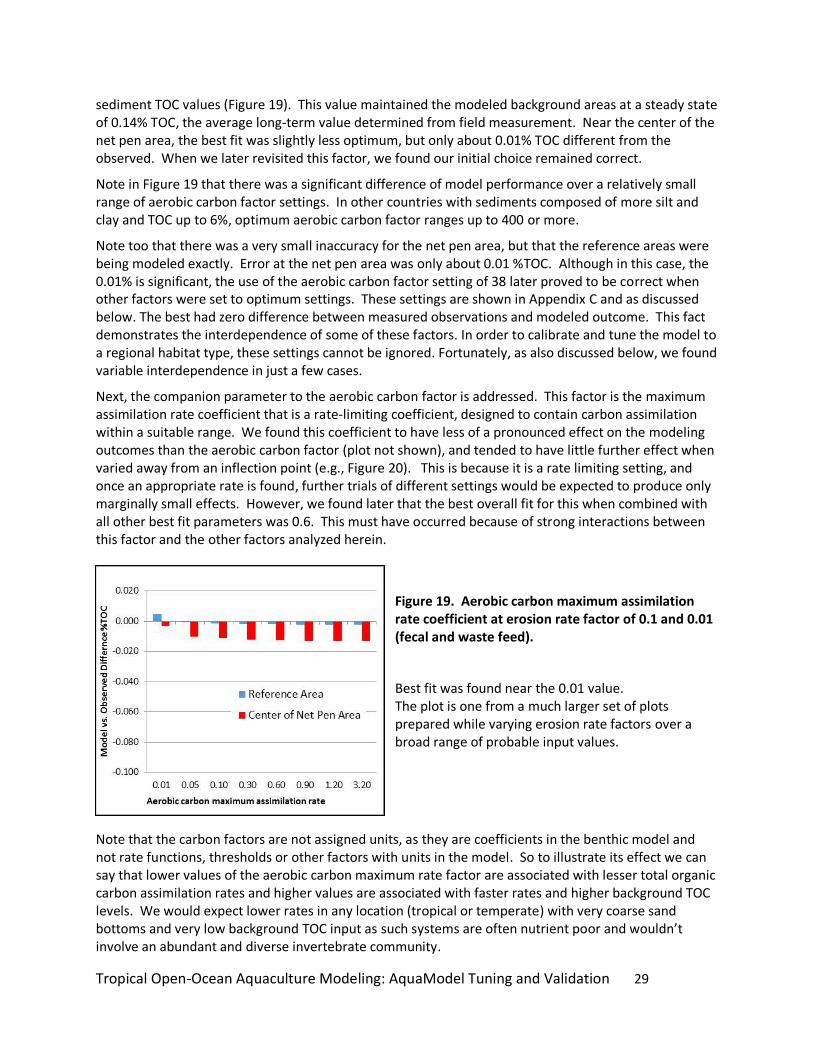
Tropical Open-Ocean Aquaculture Modeling: AquaModel Tuning and Validation 29
sediment TOC values (Figure 19). This value maintained the modeled background areas at a steady state of 0.14% TOC, the average long-term value determined from field measurement. Near the center of the net pen area, the best fit was slightly less optimum, but only about 0.01% TOC different from the observed. When we later revisited this factor, we found our initial choice remained correct.
Note in Figure 19 that there was a significant difference of model performance over a relatively small range of aerobic carbon factor settings. In other countries with sediments composed of more silt and clay and TOC up to 6%, optimum aerobic carbon factor ranges up to 400 or more.
Note too that there was a very small inaccuracy for the net pen area, but that the reference areas were being modeled exactly. Error at the net pen area was only about 0.01 %TOC. Although in this case, the 0.01% is significant, the use of the aerobic carbon factor setting of 38 later proved to be correct when other factors were set to optimum settings. These settings are shown in Appendix C and as discussed below. The best had zero difference between measured observations and modeled outcome. This fact demonstrates the interdependence of some of these factors. In order to calibrate and tune the model to a regional habitat type, these settings cannot be ignored. Fortunately, as also discussed below, we found variable interdependence in just a few cases.
Next, the companion parameter to the aerobic carbon factor is addressed. This factor is the maximum assimilation rate coefficient that is a rate-limiting coefficient, designed to contain carbon assimilation within a suitable range. We found this coefficient to have less of a pronounced effect on the modeling outcomes than the aerobic carbon factor (plot not shown), and tended to have little further effect when varied away from an inflection point (e.g., Figure 20). This is because it is a rate limiting setting, and once an appropriate rate is found, further trials of different settings would be expected to produce only marginally small effects. However, we found later that the best overall fit for this when combined with all other best fit parameters was 0.6. This must have occurred because of strong interactions between this factor and the other factors analyzed herein.
Figure 19. Aerobic carbon maximum assimilation rate coefficient at erosion rate factor of 0.1 and 0.01 (fecal and waste feed).
Best fit was found near the 0.01 value. The plot is one from a much larger set of plots prepared while varying erosion rate factors over a broad range of probable input values.
Note that the carbon factors are not assigned units, as they are coefficients in the benthic model and not rate functions, thresholds or other factors with units in the model. So to illustrate its effect we can say that lower values of the aerobic carbon maximum rate factor are associated with lesser total organic carbon assimilation rates and higher values are associated with faster rates and higher background TOC levels. We would expect lower rates in any location (tropical or temperate) with very coarse sand bottoms and very low background TOC input as such systems are often nutrient poor and wouldn’t involve an abundant and diverse invertebrate community.

Tropical Open-Ocean Aquaculture Modeling: AquaModel Tuning and Validation 30
In a separate AquaModel validation project we are conducting of a much larger fish farm in North America with background sediment TOC concentration twice as high as the Hawai’i location, we found a best fit of aerobic carbon factor of 61, about 60% higher than the value of 38 found for this study. We expected a much higher value than in Hawaii as there was >20% fines in the sediment versus almost none in Hawai’i. Moreover, the mean current velocity was significantly less. TOC concentrations are positively correlated with the percent fines in sediments and inversely correlated with current velocity near the sea bottom except in areas where rivers introduce sticky sediments that are bound together with electrical charges. When TOC is used is a performance standard for net pens, such as in Washington State, it is important to concurrently collect sediment grain size and TOC samples, as has been done at the project site for several years. Other regions such as Atlantic Canada and the country of Chile also use organic matter as an indicator of net pen enrichment, although in those cases it is sediment total volatile solids that include TOC as well as other forms of organic matter.
After determining the aerobic carbon factor, next step in model calibration is to add the known amount of fish biomass and observe the effects under and near the cages modeled, and compare that with measured field data. There was no effect of varying the anaerobic carbon factor. As discussed above, no significant numbers of anaerobic organisms would be expected given the well-aerated, coarse sand nature of this site.
In regions or sites with higher concentrations of sediment TOC (e.g., > 2.0%), the maximum erosion rate constant can be varied, particularly for waste feed, to achieve the correct and concurrent background and net pen area results. In eutrophic sea bottom areas, where anaerobic carbon decomposition is a factor, this may be increased or decreased in a stepwise fashion until the desired outcome is achieved.
The reader is reminded that normal operation of AquaModel does not involve any of these tuning or validation steps if the application location is similar to the validation location. For example, if regional validation is at a site that is predominantly sand, other sandy sites with similar sediment size frequency distributions are applicable. However, in this case moving to a site in the same region with mostly silt and clay will require some modifications. In the present case it would apply to most all leeward areas of the Hawai’ian Islands.
Erosion Rate Coefficients
A second important factor controlling the outcome of the sediment total organic carbon simulation is the erosion rate constant (or k, for constant), measured in grams carbon per meter square per day. This factor would not play a major role if the intended habitat to be modeled was completely depositional (i.e., had slow near-bottom currents never exceeding about 6 cm s-1). However, many modern net pen sites such as the Blue Ocean Mariculture facility have current velocities that allow resuspension on a regular basis.
When current speeds exceed the separate thresholds of particle resuspension for waste feed and fish feces, then particle resuspension and “erosion” occurs. We use the term erosion here to differentiate this part of the process from the resuspension, although they are interlinked processes. In AquaModel, these processes are regulated by a series of interlinked equations sensitive to the velocity thresholds (discussed below) and erosion rate. For strong current sites, this means that particulate TOC is resuspended and transported while being oxygenated to allow bacterial or infauna use of the particulate TOC (also known as POC) as food. For depositional sites, where near sea bottom currents are normally slow at all times, this constant does not play a role. In higher current areas where benthic sediment resuspension occurs regularly, this constant works to transport sediment TOC away from any given location and reduces the TOC concentration accordingly.
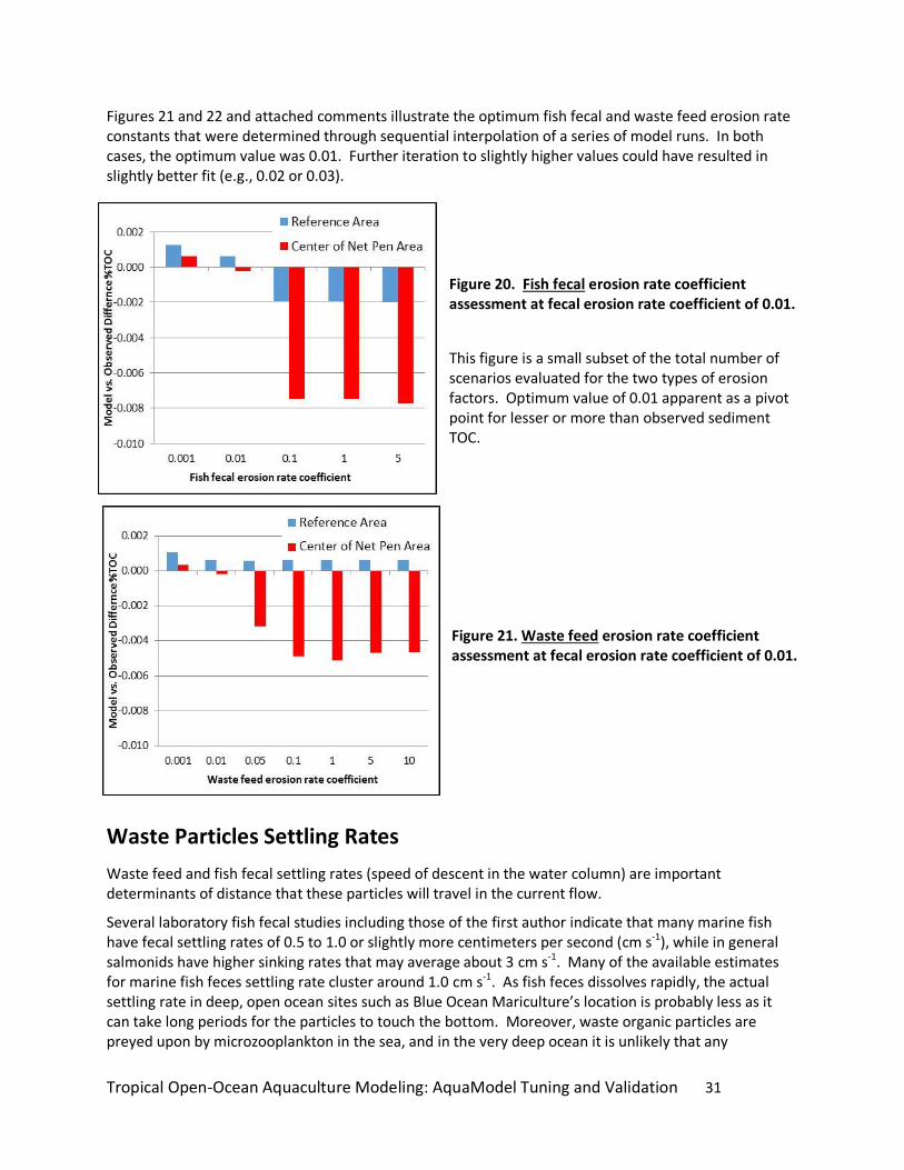
Tropical Open-Ocean Aquaculture Modeling: AquaModel Tuning and Validation 31
Figures 21 and 22 and attached comments illustrate the optimum fish fecal and waste feed erosion rate constants that were determined through sequential interpolation of a series of model runs. In both cases, the optimum value was 0.01. Further iteration to slightly higher values could have resulted in slightly better fit (e.g., 0.02 or 0.03).
Figure 20. Fish fecal erosion rate coefficient assessment at fecal erosion rate coefficient of 0.01.
This figure is a small subset of the total number of scenarios evaluated for the two types of erosion factors. Optimum value of 0.01 apparent as a pivot point for lesser or more than observed sediment TOC.
Figure 21. Waste feed erosion rate coefficient assessment at fecal erosion rate coefficient of 0.01.
Waste Particles Settling Rates
Waste feed and fish fecal settling rates (speed of descent in the water column) are important determinants of distance that these particles will travel in the current flow.
Several laboratory fish fecal studies including those of the first author indicate that many marine fish have fecal settling rates of 0.5 to 1.0 or slightly more centimeters per second (cm s-1), while in general salmonids have higher sinking rates that may average about 3 cm s-1. Many of the available estimates for marine fish feces settling rate cluster around 1.0 cm s-1. As fish feces dissolves rapidly, the actual settling rate in deep, open ocean sites such as Blue Ocean Mariculture’s location is probably less as it can take long periods for the particles to touch the bottom. Moreover, waste organic particles are preyed upon by microzooplankton in the sea, and in the very deep ocean it is unlikely that any

Tropical Open-Ocean Aquaculture Modeling: AquaModel Tuning and Validation 32
significant amount of fish fecal or waste feed arrives at the sea bottom undisturbed, but rather as zooplankton, fish or other organism’s fecal pellets with yet lower TOC content. However, for now, we use the estimates available in the literature that do not account for these other factors, while noting that this makes our calculations very conservative.
The uncertainty about sinking rates includes the fact that fish fecal particles are not uniform in size or sinking rate distribution but may exhibit a bimodal distribution as reported by some (Tlusty et al. 2000, Magill et al. 2006) or a skewed, asymmetrical distribution (our laboratory data presented in O’Brien et al. 2011). Although this particular project did not involve measurement of fish fecal settling rates, we varied the setting while keeping other optimum variable settings, and found clearly that the optimum value occurred at exactly the optimum expected value of 1.0 cm s-1 (Figure 23), exactly as we hypothesized. It is unlikely that this is coincidental, but we will continue to model this important parameter for future validation projects to look for links and correlations with varying conditions such as site depth.
Figure 22. Model evaluation of fish fecal settling rate on model vs. observed TOC differences for simulations conducted with other optimum settings.
Optimum rate of 1.0 cm s-1 produced a very good fit and conformed well with literature estimates and our prior best estimates.
Deposition and Resuspension Thresholds
Deposition and resuspension threshold constants are average values of near-sea-bottom current velocity used to trigger the deposition or resuspension of these waste particles on the sea bottom. When the current moves below or above these thresholds, AquaModel is enabled to allow these processes to occur in a proportional basis related to current strength. These threshold values maybe estimated from literature reports and some common sense regarding what we know about their density and sinking rates. They are also in line with estimates the primary author has made while Scuba diving at net pen sites with a near bottom current meter (Price Pigmy AA) operating at several net pen sites.
See the review by Reid et al. (2009), Cromey et al. (2002a, 2002b) and numerous AquaModel technical reports online for further details. Results of this study are shown in Figure 24 indicating that 8 cm s-1 produces the optimum fit. However, the overall range of effect was small for the Blue Ocean Mariculture site.
Optimum value for waste feed deposition threshold was 8 cm s-1 as expected for the net pen area where waste feed occurs (Figure 24). No trend was noted or expected for the reference area as waste feed never occurs that far from the net pens, so any result would be immaterial. Also, note the relatively small degree of effect over the range of probable values that is related to the minimal amount of deposition occurring at or near the study site in Hawai’i. Waste feed deposition threshold is likely to be
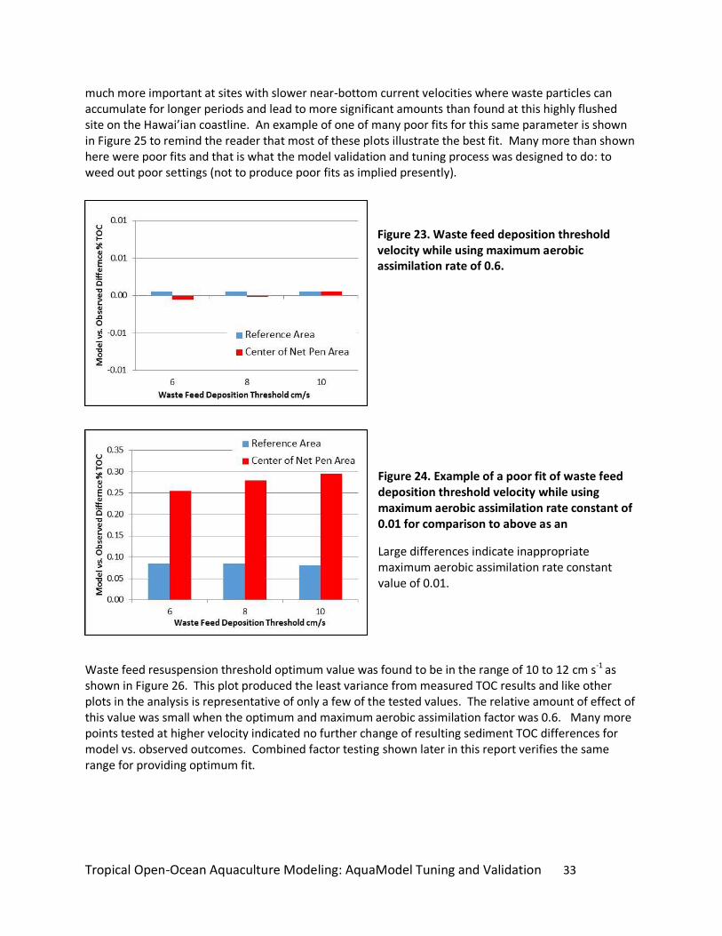
Tropical Open-Ocean Aquaculture Modeling: AquaModel Tuning and Validation 33
much more important at sites with slower near-bottom current velocities where waste particles can accumulate for longer periods and lead to more significant amounts than found at this highly flushed site on the Hawai’ian coastline. An example of one of many poor fits for this same parameter is shown in Figure 25 to remind the reader that most of these plots illustrate the best fit. Many more than shown here were poor fits and that is what the model validation and tuning process was designed to do: to weed out poor settings (not to produce poor fits as implied presently).
Figure 23. Waste feed deposition threshold velocity while using maximum aerobic assimilation rate of 0.6.
Figure 24. Example of a poor fit of waste feed deposition threshold velocity while using maximum aerobic assimilation rate constant of 0.01 for comparison to above as an
Large differences indicate inappropriate maximum aerobic assimilation rate constant value of 0.01.
Waste feed resuspension threshold optimum value was found to be in the range of 10 to 12 cm s-1 as shown in Figure 26. This plot produced the least variance from measured TOC results and like other plots in the analysis is representative of only a few of the tested values. The relative amount of effect of this value was small when the optimum and maximum aerobic assimilation factor was 0.6. Many more points tested at higher velocity indicated no further change of resulting sediment TOC differences for model vs. observed outcomes. Combined factor testing shown later in this report verifies the same range for providing optimum fit.
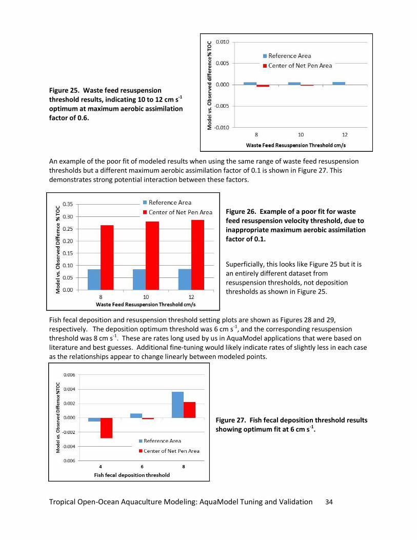
Tropical Open-Ocean Aquaculture Modeling: AquaModel Tuning and Validation 34
Figure 25. Waste feed resuspension threshold results, indicating 10 to 12 cm s-1 optimum at maximum aerobic assimilation factor of 0.6.
An example of the poor fit of modeled results when using the same range of waste feed resuspension thresholds but a different maximum aerobic assimilation factor of 0.1 is shown in Figure 27. This demonstrates strong potential interaction between these factors.
Figure 26. Example of a poor fit for waste feed resuspension velocity threshold, due to inappropriate maximum aerobic assimilation factor of 0.1.
Superficially, this looks like Figure 25 but it is an entirely different dataset from resuspension thresholds, not deposition thresholds as shown in Figure 25.
Fish fecal deposition and resuspension threshold setting plots are shown as Figures 28 and 29, respectively. The deposition optimum threshold was 6 cm s-1, and the corresponding resuspension threshold was 8 cm s-1. These are rates long used by us in AquaModel applications that were based on literature and best guesses. Additional fine-tuning would likely indicate rates of slightly less in each case as the relationships appear to change linearly between modeled points.
Figure 27. Fish fecal deposition threshold results showing optimum fit at 6 cm s-1.
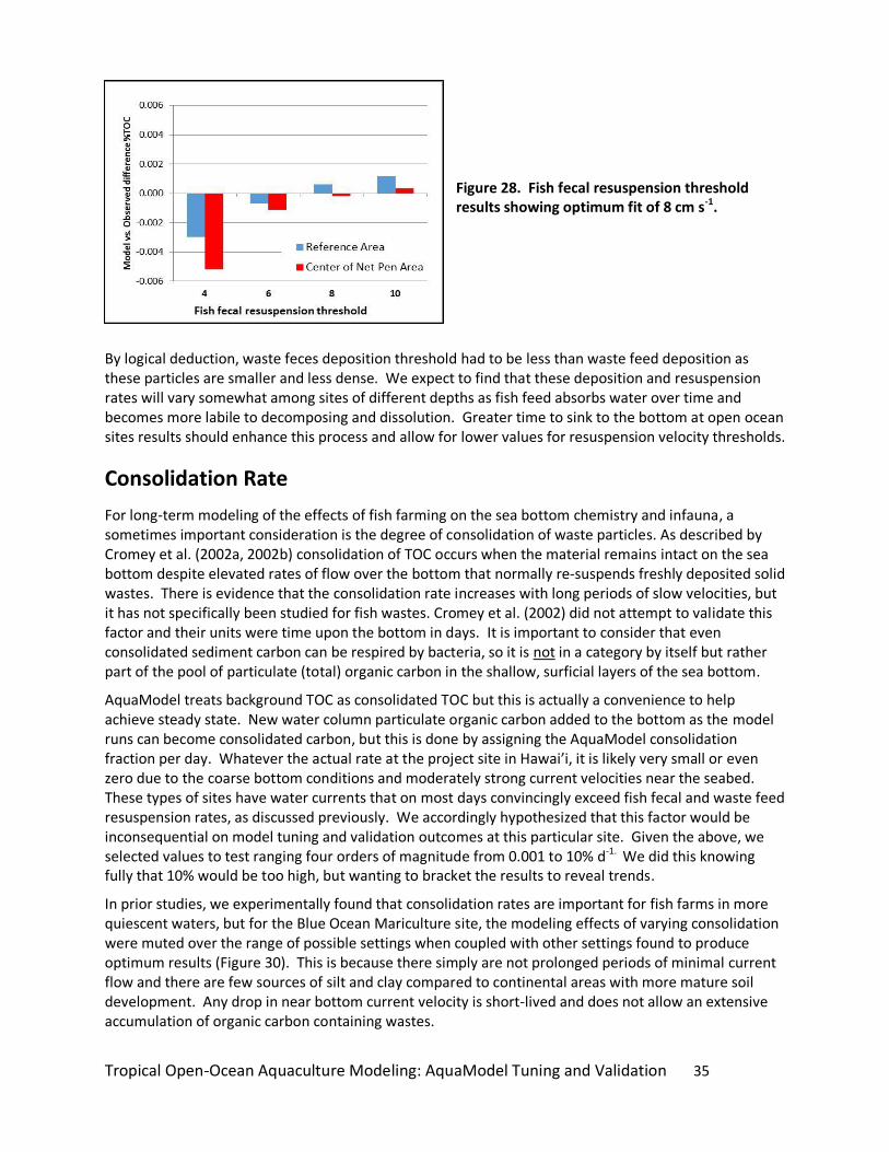
Tropical Open-Ocean Aquaculture Modeling: AquaModel Tuning and Validation 35
Figure 28. Fish fecal resuspension threshold results showing optimum fit of 8 cm s-1.
By logical deduction, waste feces deposition threshold had to be less than waste feed deposition as these particles are smaller and less dense. We expect to find that these deposition and resuspension rates will vary somewhat among sites of different depths as fish feed absorbs water over time and becomes more labile to decomposing and dissolution. Greater time to sink to the bottom at open ocean sites results should enhance this process and allow for lower values for resuspension velocity thresholds.
Consolidation Rate
For long-term modeling of the effects of fish farming on the sea bottom chemistry and infauna, a sometimes important consideration is the degree of consolidation of waste particles. As described by Cromey et al. (2002a, 2002b) consolidation of TOC occurs when the material remains intact on the sea bottom despite elevated rates of flow over the bottom that normally re-suspends freshly deposited solid wastes. There is evidence that the consolidation rate increases with long periods of slow velocities, but it has not specifically been studied for fish wastes. Cromey et al. (2002) did not attempt to validate this factor and their units were time upon the bottom in days. It is important to consider that even consolidated sediment carbon can be respired by bacteria, so it is not in a category by itself but rather part of the pool of particulate (total) organic carbon in the shallow, surficial layers of the sea bottom.
AquaModel treats background TOC as consolidated TOC but this is actually a convenience to help achieve steady state. New water column particulate organic carbon added to the bottom as the model runs can become consolidated carbon, but this is done by assigning the AquaModel consolidation fraction per day. Whatever the actual rate at the project site in Hawai’i, it is likely very small or even zero due to the coarse bottom conditions and moderately strong current velocities near the seabed. These types of sites have water currents that on most days convincingly exceed fish fecal and waste feed resuspension rates, as discussed previously. We accordingly hypothesized that this factor would be inconsequential on model tuning and validation outcomes at this particular site. Given the above, we selected values to test ranging four orders of magnitude from 0.001 to 10% d-1. We did this knowing fully that 10% would be too high, but wanting to bracket the results to reveal trends.
In prior studies, we experimentally found that consolidation rates are important for fish farms in more quiescent waters, but for the Blue Ocean Mariculture site, the modeling effects of varying consolidation were muted over the range of possible settings when coupled with other settings found to produce optimum results (Figure 30). This is because there simply are not prolonged periods of minimal current flow and there are few sources of silt and clay compared to continental areas with more mature soil development. Any drop in near bottom current velocity is short-lived and does not allow an extensive accumulation of organic carbon containing wastes.
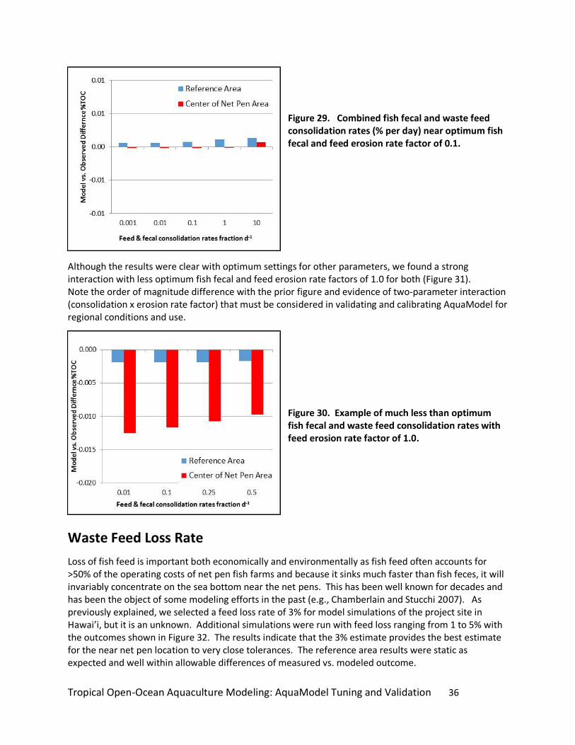
Tropical Open-Ocean Aquaculture Modeling: AquaModel Tuning and Validation 36
Figure 29. Combined fish fecal and waste feed consolidation rates (% per day) near optimum fish fecal and feed erosion rate factor of 0.1.
Although the results were clear with optimum settings for other parameters, we found a strong interaction with less optimum fish fecal and feed erosion rate factors of 1.0 for both (Figure 31). Note the order of magnitude difference with the prior figure and evidence of two-parameter interaction (consolidation x erosion rate factor) that must be considered in validating and calibrating AquaModel for regional conditions and use.
Figure 30. Example of much less than optimum fish fecal and waste feed consolidation rates with feed erosion rate factor of 1.0.
Waste Feed Loss Rate
Loss of fish feed is important both economically and environmentally as fish feed often accounts for >50% of the operating costs of net pen fish farms and because it sinks much faster than fish feces, it will invariably concentrate on the sea bottom near the net pens. This has been well known for decades and has been the object of some modeling efforts in the past (e.g., Chamberlain and Stucchi 2007). As previously explained, we selected a feed loss rate of 3% for model simulations of the project site in Hawai’i, but it is an unknown. Additional simulations were run with feed loss ranging from 1 to 5% with the outcomes shown in Figure 32. The results indicate that the 3% estimate provides the best estimate for the near net pen location to very close tolerances. The reference area results were static as expected and well within allowable differences of measured vs. modeled outcome.

Tropical Open-Ocean Aquaculture Modeling: AquaModel Tuning and Validation 37
These results are not entirely independent of model tuning effects. We could have selected values of two or four percent waste feed loss rates and achieved acceptable results. Nevertheless, the best estimate was three percent loss rate and there was no bias introduced into this estimate. We knew in advance that varying this factor was important, and also that it would affect the pen areas most, but we had no assurances that the selected feed loss rate value would interact so exactly with the other parameters to produce this outcome.
Figure 31. Feed loss rate simulations ranging from 1 to 5% showing optimum rate at 3%.
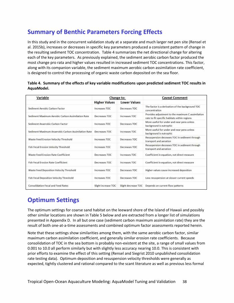
Tropical Open-Ocean Aquaculture Modeling: AquaModel Tuning and Validation 38
Summary of Benthic Parameters Forcing Effects
In this study and in the concurrent validation study at a separate and much larger net pen site (Rensel et al. 2015b), increases or decreases in specific key parameters produced a consistent pattern of change in the resulting sediment TOC concentration. Table 4 summarizes the net directional change for altering each of the key parameters. As previously explained, the sediment aerobic carbon factor produced the most change pro rata and higher values resulted in increased sediment TOC concentrations. This factor, along with its companion variable, the sediment maximum aerobic carbon assimilation rate coefficient, is designed to control the processing of organic waste carbon deposited on the sea floor. Table 4. Summary of the effects of key variable modifications upon predicted sediment TOC results in AquaModel.
Optimum Settings
The optimum settings for coarse sand habitat on the leeward shore of the Island of Hawaii and possibly other similar locations are shown in Table 5 below and are extracted from a longer list of simulations presented in Appendix D. In all but one case (sediment carbon maximum assimilation rate) they are the result of both one-at-a-time assessments and combined optimum factor assessments reported herein.
Note that these settings show similarities among them, with the same aerobic carbon factor, similar maximum carbon assimilation coefficient, and generally similar erosion rate coefficients. Because consolidation of TOC in the sea bottom is probably non-existent at the site, a range of small values from 0.001 to 10.0 all perform similarly but with slightly less accuracy nearing 10.0. This is consistent with prior efforts to examine the effect of this setting (Rensel and Siegrist 2010 unpublished consolidation rate testing data). Optimum deposition and resuspension velocity thresholds were generally as expected, tightly clustered and rational compared to the scant literature as well as previous less formal
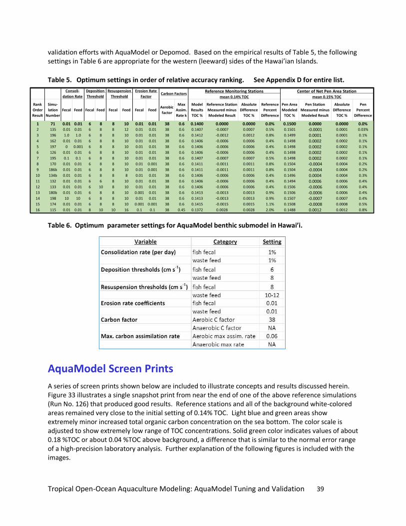
Tropical Open-Ocean Aquaculture Modeling: AquaModel Tuning and Validation 39
Rank
Order
Result
Simu-
lation
Number
Fecal Feed Fecal Feed Fecal Feed Fecal FeedAerobic
factor
Max
Assim.
Rate k
Model
Results
TOC %
Reference Station
Measured minus
Modeled Result
Absolute
Difference
TOC %
Reference
Percent
Difference
Pen Area
Modeled
TOC %
Pen Station
Measured minus
Modeled Result
Absolute
Difference
TOC %
Pen
Percent
Difference
1 71 0.01 0.01 6 8 8 10 0.01 0.01 38 0.6 0.1400 0.0000 0.0000 0.0% 0.1500 0.0000 0.0000 0.0%2 135 0.01 0.01 6 8 8 12 0.01 0.01 38 0.6 0.1407 -0.0007 0.0007 0.5% 0.1501 -0.0001 0.0001 0.03%
3 196 1.0 1.0 6 8 8 10 0.01 0.01 38 0.6 0.1412 -0.0012 0.0012 0.8% 0.1499 0.0001 0.0001 0.1%
4 162 0.01 0.01 6 8 8 10 0.01 0.01 38 0.6 0.1406 -0.0006 0.0006 0.4% 0.1498 0.0002 0.0002 0.1%
5 197 0 0.001 6 8 8 10 0.01 0.01 38 0.6 0.1406 -0.0006 0.0006 0.4% 0.1498 0.0002 0.0002 0.1%
6 126 0.01 0.01 6 8 8 10 0.01 0.01 38 0.6 0.1406 -0.0006 0.0006 0.4% 0.1498 0.0002 0.0002 0.1%
7 195 0.1 0.1 6 8 8 10 0.01 0.01 38 0.6 0.1407 -0.0007 0.0007 0.5% 0.1498 0.0002 0.0002 0.1%
8 170 0.01 0.01 6 8 8 10 0.01 0.001 38 0.6 0.1411 -0.0011 0.0011 0.8% 0.1504 -0.0004 0.0004 0.2%
9 186b 0.01 0.01 6 8 8 10 0.01 0.001 38 0.6 0.1411 -0.0011 0.0011 0.8% 0.1504 -0.0004 0.0004 0.2%
10 134b 0.01 0.01 6 8 8 8 0.01 0.01 38 0.6 0.1406 -0.0006 0.0006 0.4% 0.1496 0.0004 0.0004 0.3%
11 132 0.01 0.01 6 6 8 10 0.01 0.01 38 0.6 0.1406 -0.0006 0.0006 0.4% 0.1494 0.0006 0.0006 0.4%
12 133 0.01 0.01 6 10 8 10 0.01 0.01 38 0.6 0.1406 -0.0006 0.0006 0.4% 0.1506 -0.0006 0.0006 0.4%
13 180b 0.01 0.01 6 8 8 10 0.001 0.01 38 0.6 0.1413 -0.0013 0.0013 0.9% 0.1506 -0.0006 0.0006 0.4%
14 198 10 10 6 8 8 10 0.01 0.01 38 0.6 0.1413 -0.0013 0.0013 0.9% 0.1507 -0.0007 0.0007 0.4%
15 174 0.01 0.01 6 8 8 10 0.001 0.001 38 0.6 0.1415 -0.0015 0.0015 1.1% 0.1508 -0.0008 0.0008 0.5%
16 115 0.01 0.01 8 10 10 16 0.1 0.1 38 0.45 0.1372 0.0028 0.0028 2.0% 0.1488 0.0012 0.0012 0.8%
Center of Net Pen Area Station mean 0.15% TOC
Reference Monitoring Stations mean 0.14% TOC
Consoli-
dation Rate
Deposition
Threshold
Resuspension
Threshold
Erosion Rate
FactorCarbon Factors
validation efforts with AquaModel or Depomod. Based on the empirical results of Table 5, the following settings in Table 6 are appropriate for the western (leeward) sides of the Hawai’ian Islands.
Table 5. Optimum settings in order of relative accuracy ranking. See Appendix D for entire list.
Table 6. Optimum parameter settings for AquaModel benthic submodel in Hawai’i.
AquaModel Screen Prints
A series of screen prints shown below are included to illustrate concepts and results discussed herein. Figure 33 illustrates a single snapshot print from near the end of one of the above reference simulations (Run No. 126) that produced good results. Reference stations and all of the background white-colored areas remained very close to the initial setting of 0.14% TOC. Light blue and green areas show extremely minor increased total organic carbon concentration on the sea bottom. The color scale is adjusted to show extremely low range of TOC concentrations. Solid green color indicates values of about 0.18 %TOC or about 0.04 %TOC above background, a difference that is similar to the normal error range of a high-precision laboratory analysis. Further explanation of the following figures is included with the images.

Tropical Open-Ocean Aquaculture Modeling: AquaModel Tuning and Validation 40
Figure 32. Screen print from near end of the simulation that includes explanations.

Tropical Open-Ocean Aquaculture Modeling: AquaModel Tuning and Validation 41
Figure 33. Screen print from near end of the simulation that includes explanations identical to prior figure except color scale range increased by 0.02% TOC. Compare this figure with the prior one to show how finely tuned the model can be to illustrate these tiny amounts of sediment TOC.
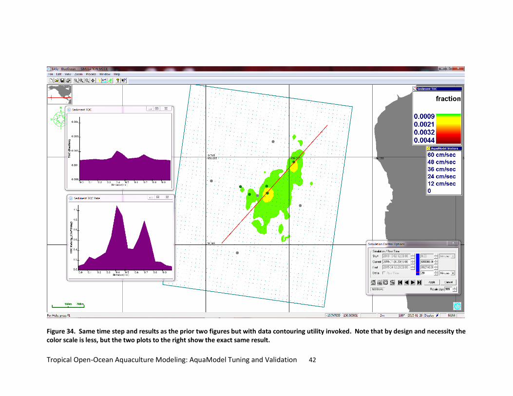
Tropical Open-Ocean Aquaculture Modeling: AquaModel Tuning and Validation 42
Figure 34. Same time step and results as the prior two figures but with data contouring utility invoked. Note that by design and necessity the color scale is less, but the two plots to the right show the exact same result.

Tropical Open-Ocean Aquaculture Modeling: AquaModel Tuning and Validation 43
Figure 35. AquaModel with visual “track waste” utility shown turned on. The purple circles illustrate the distribution of waste feed, the olive green circles indicate the pathways of fish feces as they descend to the sea bottom within the modeling domain.
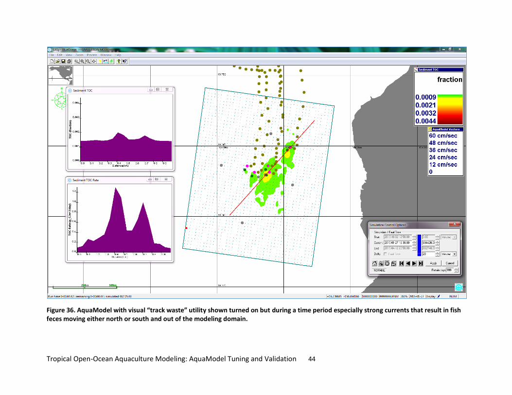
Tropical Open-Ocean Aquaculture Modeling: AquaModel Tuning and Validation 44
Figure 36. AquaModel with visual “track waste” utility shown turned on but during a time period especially strong currents that result in fish feces moving either north or south and out of the modeling domain.
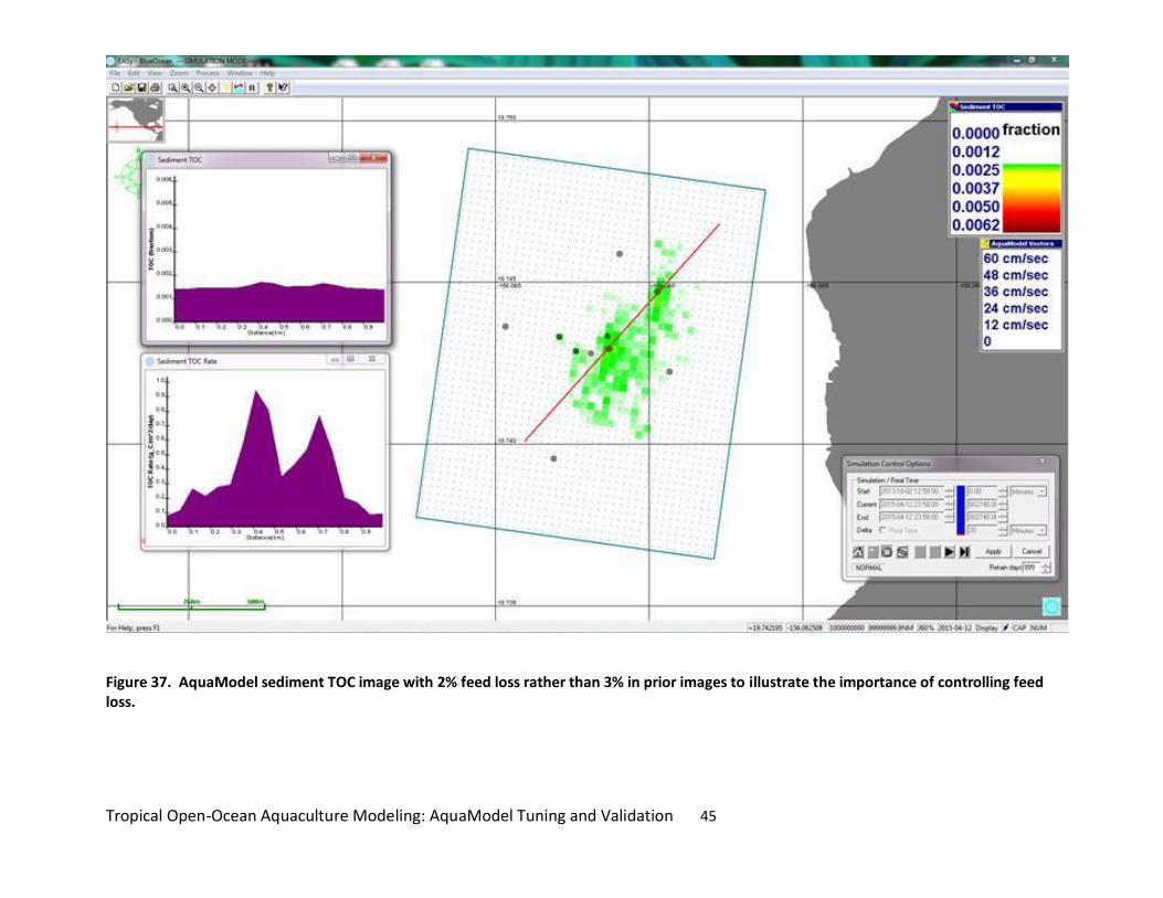
Tropical Open-Ocean Aquaculture Modeling: AquaModel Tuning and Validation 45
Figure 37. AquaModel sediment TOC image with 2% feed loss rather than 3% in prior images to illustrate the importance of controlling feed loss.

Tropical Open-Ocean Aquaculture Modeling: AquaModel Tuning and Validation 46
Other screen prints include Figure 34 that illustrates AquaModel’s built-in data and imagery contouring system that is easily invoked by a model user. Compare this figure with the prior Figure 33. Figures 35 and 36 illustrate when current flows are modestly strong (Figure 35) that the waste tracking system shows waste organic carbon containing particles being distributed within the model domain and in Figure 36, outside the modeling domain. The latter is less frequent then the former and would result in no measurable change to the sediment chemistry or biology. Figure 38 illustrates the profound effect of changing the feed loss rate from 3% to 2% for the sediment TOC concentration near the pens. Compare Figure 33 with Figure 38 to see the difference that is restricted to the near pen locations.
Summary
This study was the first formal validation study for AquaModel’s benthic submodel. The study project location was in relatively deep water with modestly strong currents that result in minimal modeled or measured effects on the sea bottom. With a long-term monitoring database, the background and probable near pen concentrations of sediment TOC were estimated. A range of modeling inputs were tested based on literature, prior modeling work, research and monitoring experience of the primary author. This optimization process relied first on evaluation of one or two parameter-at- a-time estimates and concurrent assessments with all parameters at once in model simulation runs. These model runs included 215 each, two-year simulations that lasted about 8 hours each.
As a result of the simulations and analysis it was demonstrated that certain model settings exist that were capable of hindcasting the field measurements within a very close error tolerance. Sixteen of the simulations produced results for the near cage location within 1% of the measured value. All sixteen of these simulations had similar settings that varied only slightly except for sediment consolidation rate. This was expected as water currents are moderately strong and sediments are composed of coarse sand with almost no silt or clay. In such environments, it is unreasonable to expect sediment build up or consolidation of fish farm particulate wastes and therefore consolidation settings become unimportant.
A self-criticism of this study is that there was only one sampling station near the pens to complement the four background area sampling stations. This condition results in an easier fit than had there had been many sampling stations. However, we examined the range of effects near to the existing sampling station and made projections of likely results nearby. Given the current vector rose distributions and patterns of waste particle touchdown on the sediments (shown as “TOC rate” function) in this report, one would expect if any measurable effects could be found, they would be near the net pens. Current flows were more or less balanced in north and south as well as east and west directions. In other validation studies in other countries, we have up to 20 field stations near very large net pen operations, and the model continues to produce relatively good correspondence between observed and modeled results that are statistically significant. These additional studies are in different stages of completion but helped inform us regard validity of trends we had been observing with the Blue Ocean Mariculture site model results. A report on one of these locations with much more detail on new modeling innovations and utilities used there and in the Blue Ocean Mariculture study will be available in the first half of 2015 to complement this report (Rensel et al. 2015b).
Tropical Open-Ocean Aquaculture Modeling: AquaModel Tuning and Validation 47
Literature Cited
Bianchi, T. 2006. Biochemistry of Estuaries. Oxford University Press. 720 p.
Blue Ocean Mariculture LLC. (2014). Draft Environmental Assessment for a Production Capacity Increase at the Existing Open Ocean Mariculture Site off Unualoha Point, Hawaii. Prepared for: Department of Land & Natural Resources, Office of Conservation and Coastal Lands. U.S. Army Corps of Engineers. Blue Ocean Mariculture LLC. Kailua-Kona, HI. 64 pp.
Chamberlain, J. and D. Stucchi. 2007. Simulating the effects of parameter uncertainty on waste model predictions of marine finfish aquaculture. Aquaculture 272: 296-311.
Cromey, C.J., T.D. Nickell, and K.D. Black. 2002a. DEPOMOD - Modelling the deposition and biological effects of waste solids from marine cage farms. Aquaculture 214: 211-239. Cromey, C. J., T.D. Nickell, K.D. Black, P.G. Provost, and C.R. Griffiths. 2002b. Validation of a fish farm waste resuspension model by use of a particulate tracer discharged from a point source in a coastal environment. Estuaries 25: 916-929.
DFO. 2012. Review of Depomod Predictions Versus Observations of Sulfide Concentrations Around Five Salmon Aquaculture Sites in Southwest New Brunswick. DFO Can. Sci. Advis. Sec. Sci. Advis. Rep. 2012/042.
Emerson, S. and J. Hedges. 2008. Chemical oceanography and the marine carbon cycle. Cambridge University Press. 462 pp.
EPA. 2002. Guidance for quality assurance project plans for modeling. EPA QA/G-5M. EPA/240/R-02/007 Office of Environmental Information. Washington DC. 98 p. and appendices.
Findlay, R.H. and L. Watling, L. 1997. Prediction of benthic impact of salmon net-pens based on the balance of benthic oxygen supply and demand. Mar. Ecol. Pro. Ser. 155:147-157.
Hansen, L.S. and T.H. Blackburn. 1991. Aerobic and anaerobic mineralization of organic material in marine sediment microcosms. Mar. Ecol. Prog. Ser. 75:283-291.
Lie, U., R. Evans. 1973. Long-term variability in the structure of subtidal benthic communities in Puget Sound, Washington, U.S.A. Mar. Biol. 21: 122-126
Magill, S.H,, H. Thetmeyer and C.J. Cromey. 2006. Settling velocity of faecal pellets of gilthead sea bream (Sparus aurata L.) and sea bass (Dicentrarchus labrax L.) and sensitivity analysis using measured data in a deposition model. Aquaculture 251, 295-305.
O'Brien, F., D. Kiefer and J.E. Jack Rensel. 2011. Aquamodel: Software for Sustainable Development of Open Ocean Fish Farms. U.S. Department of Agriculture: Small Business Innovation Research Final Report Prepared by System Science Applications, Inc. Irvine, CA. Circulation data provided by PacIOOS (www.pacioos.org), part of the U.S. Integrated Ocean Observing System (IOOS®), funded in part by National Oceanic and Atmospheric Administration (NOAA) Award #NA11NOS0120039. 124 p.
Pannell, D.J. 1997. Sensitivity analysis: Strategies, methods, concepts, examples. Agricultural Economics 16: 139-152.
Reid, G. K., Liutkus, M., Robinson, S. M. C., Chopin, T. R., Blair, T., Lander, T., Mullen, J., Page, F. and Moccia, R. D. 2009. A review of the biophysical properties of salmonid faeces: implications for aquaculture waste dispersal models and integrated multi-trophic aquaculture. Aquaculture Research, 40: 257–273.

Tropical Open-Ocean Aquaculture Modeling: AquaModel Tuning and Validation 48
Rensel, J.E., D.A. Kiefer and F.J. O’Brien. 2013. Initial AquaModel Study of Potential Fish Mariculture near the United Arab Emirates East Coast. Prepared by Systems Science Applications, Inc. Los Angeles for Dr. Donald Anderson, Woods Hole Oceanographic Institution and the United Arab Emirates, Ministry of Environment and Water. 77 p.
Rensel, J.E., Z. Siegrist, D.A. Kiefer and F.J. O’Brien. 2015b. AquaModel Tuning and Validation: North American Salmon Farm. Prepared by System Science Applications, Inc. for Washington and NOAA Sea Grant program. Manuscript in progress.
Stumm, W. and J.J. Morgan. 1995. Aquatic chemistry: chemical equilibria and rates in natural waters. Wiley Publishing. 1022 p.
Tlusty, M.F., K Snook, V.A. Pepper and M.R. Anderson. 2000. The potential for soluble and transport loss of particulate aquaculture wastes. Aquaculture Res. 31:745.
Westrich, J.T., Berner, R.A., 1984. The role of sedimentary organic matter in bacterial sulphate reduction: the Gmodel tested. Limnol. Oceanogr. 29, 236-249.

Tropical Open-Ocean Aquaculture Modeling: AquaModel Tuning and Validation 49
Appendix A Pen numbering system, volume, conversion to cubic geometric space and geo-position of cage center.
AquaModel Pen No.
Project Pen No.
Mid Depth (m)
Volume ( m3)
Height m Length Width Height Latitude Longitude
1 P2 15.195 3000 10.39 17 17 10.39 19.74330 -156.06292
2 P3 15.195 3000 10.39 17 17 10.39 19.74333 -156.06135
3 P4 15.195 3000 10.39 17 17 10.39 19.74287 -156.06238
4 DRA 16.08 7000 12.16 24 24 12.16 19.72105 -156.06108
5 DRB 16.08 7000 12.16 24 24 12.16 19.74293 -156.06130
Appendix B TOC Laboratory Protocols University of Hawaii Hilo.
1) Dry and weigh initial sample
2) Acidify sample to remove IC
3) Weigh dried combusted 47mm GF/F
4) Filter acidified sample onto GF/F (will take a while, rinse w/ organic free DI)
5) Dry and weigh filter + dried acidified sediment
6) Scrape dried sediment off the filter, homogenize, prepare for CHN analysis
7) Get %C of acidified sample (this is the % organic C in the acidified sediment)
8) Calculate total amount of organic C in the sample (% organic C multiplied by the mass of acidified sample)
9) Calculate total amount of organic C in the original sample (total organic C divided by the original mass of sediment, multiplied by 100%)

Tropical Open-Ocean Aquaculture Modeling: AquaModel Tuning and Validation 50
Appendix C. Table of more important single and multiple factor validation results shown in charts in this document.
Deposition and Resuspension Thresholds: Fish Feces and Waste Feed x Maximum Aerobic Assimilation Rate Coefficient
Sediment Aerobic Carbon Factor
Sediment Aerobic Carbon Maximum Assimilation Rate Coefficient

Tropical Open-Ocean Aquaculture Modeling: AquaModel Tuning and Validation 51
Fish Fecal Settling Rate
Waste Feed Erosion Rate Coefficient x Fish Fecal Erosion Rate Coefficient
Fish

Tropical Open-Ocean Aquaculture Modeling: AquaModel Tuning and Validation 52
Fecal Erosion Rate Coefficient x Waste Feed Erosion Rate Coefficient
Feed & Fecal Consolidation Rate x Feed & Fecal Erosion Rate Coefficients

Tropical Open-Ocean Aquaculture Modeling: AquaModel Tuning and Validation 53
Appendix D. List of simulation settings assessed in later part of validation study and resulting skill of model to fit a mean of 0.15% sediment TOC at the center of lease area of Blue Ocean Mariculture.
Skill expressed as a) model predicted percent TOC; b) model vs mean observed difference, c) absolute difference of b and d) overall percent difference. Total N = 210. Colored background groups different classes of optimum fit between modeled and observed results.
Consolidation
Rate Deposition Threshold
Resuspension Threshold
Erosion Rate Factor
Carbon Factors Reference Monitoring Stations (mean 0.14% TOC) Center of Net Pen Area Station (mean 0.15% TOC)
Rank Order Result
Simu-lation
Number Fecal Feed Fecal Feed Fecal Feed Fecal Feed
Aerobic Factor
Max Assim. Rate K
Model Results TOC (%)
Reference Station
Measured minus
Modeled Result
Absolute Difference
(TOC %DW)
Reference Percent
Difference
Pen Area Modeled TOC (%)
Pen Station
Measured minus
Modeled Result
Absolute Difference
(TOC %DW)
Pen Percent
Difference
1 71 0.01 0.01 6 8 8 10 0.01 0.01 38 0.6 0.1400 0.0000 0.0000 0.0% 0.1500 0.0000 0.0000 0.0%
2 135 0.01 0.01 6 8 8 12 0.01 0.01 38 0.6 0.1407 -0.0007 0.0007 0.5% 0.1501 -0.0001 0.0001 0.03%
3 196 1.0 1.0 6 8 8 10 0.01 0.01 38 0.6 0.1412 -0.0012 0.0012 0.8% 0.1499 0.0001 0.0001 0.1%
4 162 0.01 0.01 6 8 8 10 0.01 0.01 38 0.6 0.1406 -0.0006 0.0006 0.4% 0.1498 0.0002 0.0002 0.1%
5 197 0 0.001 6 8 8 10 0.01 0.01 38 0.6 0.1406 -0.0006 0.0006 0.4% 0.1498 0.0002 0.0002 0.1%
6 126 0.01 0.01 6 8 8 10 0.01 0.01 38 0.6 0.1406 -0.0006 0.0006 0.4% 0.1498 0.0002 0.0002 0.1%
7 195 0.1 0.1 6 8 8 10 0.01 0.01 38 0.6 0.1407 -0.0007 0.0007 0.5% 0.1498 0.0002 0.0002 0.1%
8 170 0.01 0.01 6 8 8 10 0.01 0.001 38 0.6 0.1411 -0.0011 0.0011 0.8% 0.1504 -0.0004 0.0004 0.2%
9 186b 0.01 0.01 6 8 8 10 0.01 0.001 38 0.6 0.1411 -0.0011 0.0011 0.8% 0.1504 -0.0004 0.0004 0.2%
10 134b 0.01 0.01 6 8 8 8 0.01 0.01 38 0.6 0.1406 -0.0006 0.0006 0.4% 0.1496 0.0004 0.0004 0.3%
11 132 0.01 0.01 6 6 8 10 0.01 0.01 38 0.6 0.1406 -0.0006 0.0006 0.4% 0.1494 0.0006 0.0006 0.4%
12 133 0.01 0.01 6 10 8 10 0.01 0.01 38 0.6 0.1406 -0.0006 0.0006 0.4% 0.1506 -0.0006 0.0006 0.4%
13 180b 0.01 0.01 6 8 8 10 0.001 0.01 38 0.6 0.1413 -0.0013 0.0013 0.9% 0.1506 -0.0006 0.0006 0.4%
14 198 10 10 6 8 8 10 0.01 0.01 38 0.6 0.1413 -0.0013 0.0013 0.9% 0.1507 -0.0007 0.0007 0.4%
15 174 0.01 0.01 6 8 8 10 0.001 0.001 38 0.6 0.1415 -0.0015 0.0015 1.1% 0.1508 -0.0008 0.0008 0.5%
16 115 0.01 0.01 8 10 10 16 0.1 0.1 38 0.45 0.1372 0.0028 0.0028 2.0% 0.1488 0.0012 0.0012 0.8%
17 127 0.01 0.01 6 8 8 10 0.01 0.01 38 0.5 0.1411 -0.0011 0.0011 0.8% 0.1516 -0.0016 0.0016 1.1%

Tropical Open-Ocean Aquaculture Modeling: AquaModel Tuning and Validation 54
Consolidation
Rate Deposition Threshold
Resuspension Threshold
Erosion Rate Factor
Carbon Factors Reference Monitoring Stations (mean 0.14% TOC) Center of Net Pen Area Station (mean 0.15% TOC)
Rank Order Result
Simu-lation
Number Fecal Feed Fecal Feed Fecal Feed Fecal Feed
Aerobic Factor
Max Assim. Rate K
Model Results TOC (%)
Reference Station
Measured minus
Modeled Result
Absolute Difference
(TOC %DW)
Reference Percent
Difference
Pen Area Modeled TOC (%)
Pen Station
Measured minus
Modeled Result
Absolute Difference
(TOC %DW)
Pen Percent
Difference
18 129 0.01 0.01 6 8 8 14 0.01 0.01 38 0.3 0.1412 -0.0012 0.0012 0.8% 0.1518 -0.0018 0.0018 1.2%
19 89 0.1 0.1 8 10 10 16 0.1 0.1 38 0.6 0.1408 -0.0008 0.0008 0.6% 0.1473 0.0027 0.0027 1.8%
20 91 0.1 0.1 8 10 10 16 0.1 0.1 38 0.6 0.1408 -0.0008 0.0008 0.6% 0.1473 0.0027 0.0027 1.8%
21 145 0.01 0.01 6 8 8 10 0.01 0.01 38 0.6 0.1391 0.0009 0.0009 0.7% 0.1471 0.0029 0.0029 1.9%
22 101 0.01 0.01 6 8 8 12 1.0 1.0 38 0.01 0.1448 -0.0048 0.0048 3.4% 0.1470 0.0030 0.0030 2.0%
23 160 0.01 0.01 6 8 8 10 0.01 0.05 38 0.6 0.1406 -0.0006 0.0006 0.4% 0.1468 0.0032 0.0032 2.1%
24 90 0.1 0.1 8 10 10 16 0.1 0.1 38 0.6 0.1371 0.0029 0.0029 2.0% 0.1463 0.0037 0.0037 2.5%
25 192 0.01 0.01 6 8 8 10 0.001 10.0 38 0.6 0.1412 -0.0012 0.0012 0.9% 0.1462 0.0038 0.0038 2.5%
26 191 0.01 0.01 6 8 8 10 0.001 0.1 38 0.6 0.1412 -0.0012 0.0012 0.9% 0.1462 0.0038 0.0038 2.6%
27 189 0.01 0.01 6 8 8 10 0.001 5 38 0.6 0.1412 -0.0012 0.0012 0.9% 0.1461 0.0039 0.0039 2.6%
28 114 0.01 0.01 8 10 10 16 0.1 0.1 38 0.3 0.1378 0.0022 0.0022 1.6% 0.1540 -0.0040 0.0040 2.7%
29 113 0.1 0.1 8 10 10 16 0.1 0.1 38 0.3 0.1378 0.0022 0.0022 1.6% 0.1540 -0.0040 0.0040 2.7%
30 92 0.1 0.1 8 10 10 16 0.1 0.1 38 0.3 0.1404 -0.0004 0.0004 0.3% 0.1542 -0.0042 0.0042 2.8%
31 194 0.01 0.01 6 8 8 10 0.0001 1 38 0.6 0.1412 -0.0012 0.0012 0.9% 0.1457 0.0043 0.0043 2.9%
32 183 0.01 0.01 6 8 8 10 0.001 1.0 38 0.6 0.1412 -0.0012 0.0012 0.9% 0.1456 0.0044 0.0044 2.9%
33 154 0.01 0.01 6 8 8 10 0.10 5.0 38 0.6 0.1405 -0.0005 0.0005 0.4% 0.1454 0.0046 0.0046 3.1%
34 177 0.01 0.01 6 8 8 10 0.01 10.0 38 0.6 0.1406 -0.0006 0.0006 0.4% 0.1454 0.0046 0.0046 3.1%
35 176 0.01 0.01 6 8 8 10 0.01 5.0 38 0.6 0.1406 -0.0006 0.0006 0.4% 0.1453 0.0047 0.0047 3.1%
36 182 0.01 0.01 6 8 8 10 0.01 0.1 38 0.6 0.1406 -0.0006 0.0006 0.4% 0.1451 0.0049 0.0049 3.3%
37 165 0.01 0.01 6 8 8 10 0.01 0.10 38 0.6 0.1406 -0.0006 0.0006 0.4% 0.1450 0.0050 0.0050 3.4%
38 158 0.01 0.01 6 8 8 10 0.01 1.00 38 0.6 0.1406 -0.0006 0.0006 0.4% 0.1449 0.0051 0.0051 3.4%
39 87 0.1 0.1 8 10 10 12 0.1 0.1 38 0.6 0.1380 0.0020 0.0020 1.4% 0.1444 0.0056 0.0056 3.7%
40 122 0.01 0.01 6 8 10 14 0.1 0.1 38 0.5 0.1371 0.0029 0.0029 2.1% 0.1437 0.0063 0.0063 4.2%
41 130 0.01 0.01 6 10 8 16 0.1 0.1 38 0.5 0.1370 0.0030 0.0030 2.1% 0.1432 0.0068 0.0068 4.5%
42 193 0.01 0.01 6 8 8 10 1.0 0.0001 38 0.6 0.1381 0.0019 0.0019 1.4% 0.1432 0.0068 0.0068 4.5%

Tropical Open-Ocean Aquaculture Modeling: AquaModel Tuning and Validation 55
Consolidation
Rate Deposition Threshold
Resuspension Threshold
Erosion Rate Factor
Carbon Factors Reference Monitoring Stations (mean 0.14% TOC) Center of Net Pen Area Station (mean 0.15% TOC)
Rank Order Result
Simu-lation
Number Fecal Feed Fecal Feed Fecal Feed Fecal Feed
Aerobic Factor
Max Assim. Rate K
Model Results TOC (%)
Reference Station
Measured minus
Modeled Result
Absolute Difference
(TOC %DW)
Reference Percent
Difference
Pen Area Modeled TOC (%)
Pen Station
Measured minus
Modeled Result
Absolute Difference
(TOC %DW)
Pen Percent
Difference
43 142 0.01 0.01 6 8 8 10 0.01 0.01 38 0.60 0.1392 0.0008 0.0008 0.5% 0.1432 0.0068 0.0068 4.5%
44 178 0.01 0.01 6 8 8 10 1.0 0.001 38 0.6 0.1381 0.0019 0.0019 1.4% 0.1432 0.0068 0.0068 4.6%
45 108 0.01 0.01 6 8 8 12 1.0 1.0 38 0.1 0.1383 0.0017 0.0017 1.2% 0.1431 0.0069 0.0069 4.6%
46 121 0.01 0.01 6 8 9 13 0.1 0.1 38 0.5 0.1371 0.0029 0.0029 2.1% 0.1428 0.0072 0.0072 4.8%
47 125 0.01 0.01 7 9 9 13 0.1 0.1 38 0.5 0.1371 0.0029 0.0029 2.1% 0.1428 0.0072 0.0072 4.8%
48 187 0.01 0.01 6 8 8 10 5.0 0.001 38 0.6 0.1381 0.0019 0.0019 1.4% 0.1428 0.0072 0.0072 4.8%
49 180 0.01 0.01 6 8 8 10 0.001 0.01 38 0.6 0.1380 0.0020 0.0020 1.4% 0.1427 0.0073 0.0073 4.9%
50 186 0.01 0.01 6 8 8 10 0.01 0.001 38 0.6 0.1380 0.0020 0.0020 1.4% 0.1427 0.0073 0.0073 4.9%
51 188 0.01 0.01 6 8 8 10 10.0 0.001 38 0.6 0.1381 0.0019 0.0019 1.4% 0.1426 0.0074 0.0074 4.9%
52 171 0.01 0.01 6 8 8 10 0.100 0.001 38 0.6 0.1375 0.0025 0.0025 1.8% 0.1426 0.0074 0.0074 4.9%
53 181 0.01 0.01 6 8 8 10 0.1 0.001 38 0.6 0.1375 0.0025 0.0025 1.8% 0.1426 0.0074 0.0074 4.9%
54 152 0.01 0.01 6 8 8 10 0.10 0.01 38 0.6 0.1381 0.0019 0.0019 1.4% 0.1425 0.0075 0.0075 5.0%
55 163 0.01 0.01 6 8 8 10 1.00 0.01 38 0.6 0.1381 0.0019 0.0019 1.4% 0.1425 0.0075 0.0075 5.0%
56 184 0.01 0.01 6 8 8 10 1.0 0.01 38 0.6 0.1381 0.0019 0.0019 1.4% 0.1425 0.0075 0.0075 5.0%
57 172 0.01 0.01 6 8 8 10 0.100 0.005 38 0.6 0.1370 0.0030 0.0030 2.2% 0.1424 0.0076 0.0076 5.1%
58 164 0.01 0.01 6 8 8 10 5.00 0.01 38 0.6 0.1380 0.0020 0.0020 1.4% 0.1423 0.0077 0.0077 5.1%
59 185 0.01 0.01 6 8 8 10 5.0 0.01 38 0.6 0.1380 0.0020 0.0020 1.4% 0.1423 0.0077 0.0077 5.1%
60 148 0.01 0.01 6 8 8 10 0.01 0.01 38 0.60 0.1380 0.0020 0.0020 1.4% 0.1422 0.0078 0.0078 5.2%
61 161 0.01 0.01 6 8 8 10 0.05 0.01 38 0.6 0.1380 0.0020 0.0020 1.4% 0.1422 0.0078 0.0078 5.2%
62 128 0.01 0.01 6 10 8 16 0.01 0.01 38 0.30 0.1430 -0.0030 0.0030 2.2% 0.1579 -0.0079 0.0079 5.2%
63 124 0.01 0.01 8 10 8 12 0.1 0.1 38 0.50 0.1370 0.0030 0.0030 2.2% 0.1417 0.0083 0.0083 5.5%
64 95 0.01 0.01 6 8 8 12 1.0 1.0 38 0.1 0.1383 0.0017 0.0017 1.2% 0.1409 0.0091 0.0091 6.1%
65 104 0.01 0.01 6 8 8 12 1.0 1.0 38 0.1 0.1383 0.0017 0.0017 1.2% 0.1409 0.0091 0.0091 6.1%
66 104b 0.01 0.01 6 8 8 12 1.0 10.0 38 0.1 0.1383 0.0017 0.0017 1.2% 0.1409 0.0091 0.0091 6.1%
67 108b 0.01 0.01 6 8 8 12 1.0 1.0 38 0.1 0.1383 0.0017 0.0017 1.2% 0.1409 0.0091 0.0091 6.1%

Tropical Open-Ocean Aquaculture Modeling: AquaModel Tuning and Validation 56
Consolidation
Rate Deposition Threshold
Resuspension Threshold
Erosion Rate Factor
Carbon Factors Reference Monitoring Stations (mean 0.14% TOC) Center of Net Pen Area Station (mean 0.15% TOC)
Rank Order Result
Simu-lation
Number Fecal Feed Fecal Feed Fecal Feed Fecal Feed
Aerobic Factor
Max Assim. Rate K
Model Results TOC (%)
Reference Station
Measured minus
Modeled Result
Absolute Difference
(TOC %DW)
Reference Percent
Difference
Pen Area Modeled TOC (%)
Pen Station
Measured minus
Modeled Result
Absolute Difference
(TOC %DW)
Pen Percent
Difference
68 123 0.01 0.01 7 9 8 12 0.1 0.1 38 0.50 0.1370 0.0030 0.0030 2.2% 0.1406 0.0094 0.0094 6.2%
69 76 0.5 0.5 6 8 8 10 1.0 1.0 38 0.6 0.1383 0.0017 0.0017 1.2% 0.1402 0.0098 0.0098 6.5%
70 119 0.01 0.01 6 8 8 12 0.1 0.1 38 0.45 0.1372 0.0028 0.0028 2.0% 0.1402 0.0098 0.0098 6.5%
71 116 0.01 0.01 6 8 8 12 0.1 0.1 38 0.45 0.1372 0.0028 0.0028 2.0% 0.1402 0.0098 0.0098 6.5%
72 61 0.01 0.01 6 8 8 10 4.0 4.0 38 1.6 0.1400 0.0000 0.0000 0.0% 0.1400 0.0100 0.0100 6.7%
73 64 0.01 0.01 6 8 8 10 4.0 4.0 38 1.6 0.1400 0.0000 0.0000 0.0% 0.1400 0.0100 0.0100 6.7%
74 66 0.01 0.01 6 8 8 10 4.0 4.0 38 3.2 0.1400 0.0000 0.0000 0.0% 0.1400 0.0100 0.0100 6.7%
75 67 0.01 0.01 6 8 8 10 4.0 4.0 38 0.6 0.1400 0.0000 0.0000 0.0% 0.1400 0.0100 0.0100 6.7%
76 68 0.01 0.01 6 8 8 10 4.0 4.0 38 0.6 0.1400 0.0000 0.0000 0.0% 0.1400 0.0100 0.0100 6.7%
77 69 0.01 0.01 6 12 8 14 4.0 4.0 38 0.6 0.1400 0.0000 0.0000 0.0% 0.1400 0.0100 0.0100 6.7%
78 72 0.01 0.01 6 8 8 10 1.0 1.0 38 0.6 0.1400 0.0000 0.0000 0.0% 0.1400 0.0100 0.0100 6.7%
79 73 0.01 0.01 6 8 8 10 10.0 10.0 38 0.6 0.1400 0.0000 0.0000 0.0% 0.1400 0.0100 0.0100 6.7%
80 118 0.01 0.01 6 8 8 12 0.1 0.1 38 0.50 0.1371 0.0029 0.0029 2.1% 0.1399 0.0101 0.0101 6.7%
81 120 0.01 0.01 6 8 8 12 0.1 0.1 38 0.55 0.1368 0.0032 0.0032 2.3% 0.1397 0.0103 0.0103 6.9%
82 200 0.01 0.01 6 8 8 12 1.0 1.0 38 0.05 0.1390 0.0010 0.0010 0.7% 0.1397 0.0103 0.0103 6.9%
83 117 0.01 0.01 6 8 8 12 0.1 0.1 38 0.60 0.1368 0.0032 0.0032 2.3% 0.1395 0.0105 0.0105 7.0%
84 159 0.01 0.01 6 8 8 10 1.00 0.05 38 0.6 0.1381 0.0019 0.0019 1.4% 0.1394 0.0106 0.0106 7.0%
85 199 0.01 0.01 6 8 8 10 1.0 1.0 38 0.05 0.1390 0.0010 0.0010 0.7% 0.1393 0.0107 0.0107 7.1%
86 111 0.01 0.01 6 8 8 12 1.0 1.0 38 0.1 0.1384 0.0016 0.0016 1.1% 0.1392 0.0108 0.0108 7.2%
87 77 0.25 0.25 6 8 8 10 1.0 1.0 38 0.6 0.1381 0.0019 0.0019 1.4% 0.1392 0.0108 0.0108 7.2%
88 112 0.01 0.01 6 8 8 12 1.0 1.0 38 0.1 0.1385 0.0015 0.0015 1.1% 0.1391 0.0109 0.0109 7.2%
89 107 0.01 0.01 6 8 8 12 1.0 1.0 38 0.1 0.1385 0.0015 0.0015 1.1% 0.1391 0.0109 0.0109 7.2%
90 109 0.01 0.01 6 8 8 12 1.0 1.0 38 0.1 0.1385 0.0015 0.0015 1.1% 0.1391 0.0109 0.0109 7.2%
91 110 0.01 0.01 6 8 8 12 1.0 1.0 38 0.1 0.1385 0.0015 0.0015 1.1% 0.1391 0.0109 0.0109 7.2%
92 95b 0.01 0.01 6 8 8 12 1.0 1.0 38 0.1 0.1385 0.0015 0.0015 1.1% 0.1391 0.0109 0.0109 7.2%
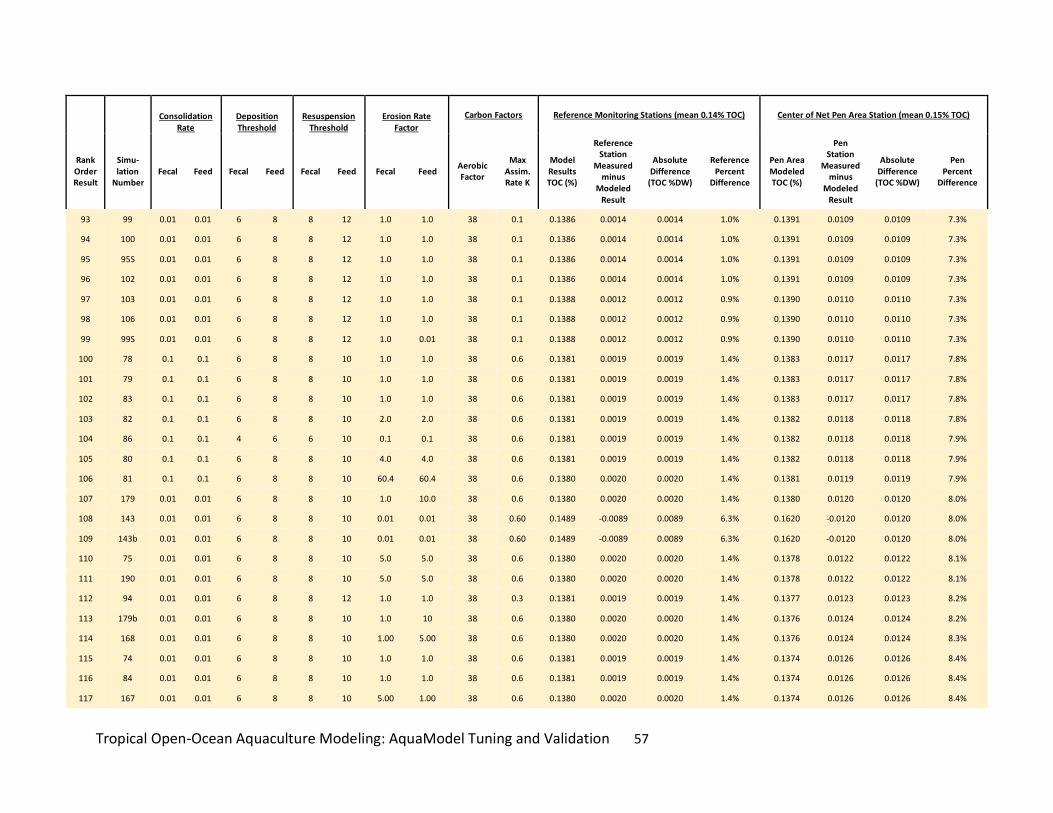
Tropical Open-Ocean Aquaculture Modeling: AquaModel Tuning and Validation 57
Consolidation
Rate Deposition Threshold
Resuspension Threshold
Erosion Rate Factor
Carbon Factors Reference Monitoring Stations (mean 0.14% TOC) Center of Net Pen Area Station (mean 0.15% TOC)
Rank Order Result
Simu-lation
Number Fecal Feed Fecal Feed Fecal Feed Fecal Feed
Aerobic Factor
Max Assim. Rate K
Model Results TOC (%)
Reference Station
Measured minus
Modeled Result
Absolute Difference
(TOC %DW)
Reference Percent
Difference
Pen Area Modeled TOC (%)
Pen Station
Measured minus
Modeled Result
Absolute Difference
(TOC %DW)
Pen Percent
Difference
93 99 0.01 0.01 6 8 8 12 1.0 1.0 38 0.1 0.1386 0.0014 0.0014 1.0% 0.1391 0.0109 0.0109 7.3%
94 100 0.01 0.01 6 8 8 12 1.0 1.0 38 0.1 0.1386 0.0014 0.0014 1.0% 0.1391 0.0109 0.0109 7.3%
95 95S 0.01 0.01 6 8 8 12 1.0 1.0 38 0.1 0.1386 0.0014 0.0014 1.0% 0.1391 0.0109 0.0109 7.3%
96 102 0.01 0.01 6 8 8 12 1.0 1.0 38 0.1 0.1386 0.0014 0.0014 1.0% 0.1391 0.0109 0.0109 7.3%
97 103 0.01 0.01 6 8 8 12 1.0 1.0 38 0.1 0.1388 0.0012 0.0012 0.9% 0.1390 0.0110 0.0110 7.3%
98 106 0.01 0.01 6 8 8 12 1.0 1.0 38 0.1 0.1388 0.0012 0.0012 0.9% 0.1390 0.0110 0.0110 7.3%
99 99S 0.01 0.01 6 8 8 12 1.0 0.01 38 0.1 0.1388 0.0012 0.0012 0.9% 0.1390 0.0110 0.0110 7.3%
100 78 0.1 0.1 6 8 8 10 1.0 1.0 38 0.6 0.1381 0.0019 0.0019 1.4% 0.1383 0.0117 0.0117 7.8%
101 79 0.1 0.1 6 8 8 10 1.0 1.0 38 0.6 0.1381 0.0019 0.0019 1.4% 0.1383 0.0117 0.0117 7.8%
102 83 0.1 0.1 6 8 8 10 1.0 1.0 38 0.6 0.1381 0.0019 0.0019 1.4% 0.1383 0.0117 0.0117 7.8%
103 82 0.1 0.1 6 8 8 10 2.0 2.0 38 0.6 0.1381 0.0019 0.0019 1.4% 0.1382 0.0118 0.0118 7.8%
104 86 0.1 0.1 4 6 6 10 0.1 0.1 38 0.6 0.1381 0.0019 0.0019 1.4% 0.1382 0.0118 0.0118 7.9%
105 80 0.1 0.1 6 8 8 10 4.0 4.0 38 0.6 0.1381 0.0019 0.0019 1.4% 0.1382 0.0118 0.0118 7.9%
106 81 0.1 0.1 6 8 8 10 60.4 60.4 38 0.6 0.1380 0.0020 0.0020 1.4% 0.1381 0.0119 0.0119 7.9%
107 179 0.01 0.01 6 8 8 10 1.0 10.0 38 0.6 0.1380 0.0020 0.0020 1.4% 0.1380 0.0120 0.0120 8.0%
108 143 0.01 0.01 6 8 8 10 0.01 0.01 38 0.60 0.1489 -0.0089 0.0089 6.3% 0.1620 -0.0120 0.0120 8.0%
109 143b 0.01 0.01 6 8 8 10 0.01 0.01 38 0.60 0.1489 -0.0089 0.0089 6.3% 0.1620 -0.0120 0.0120 8.0%
110 75 0.01 0.01 6 8 8 10 5.0 5.0 38 0.6 0.1380 0.0020 0.0020 1.4% 0.1378 0.0122 0.0122 8.1%
111 190 0.01 0.01 6 8 8 10 5.0 5.0 38 0.6 0.1380 0.0020 0.0020 1.4% 0.1378 0.0122 0.0122 8.1%
112 94 0.01 0.01 6 8 8 12 1.0 1.0 38 0.3 0.1381 0.0019 0.0019 1.4% 0.1377 0.0123 0.0123 8.2%
113 179b 0.01 0.01 6 8 8 10 1.0 10 38 0.6 0.1380 0.0020 0.0020 1.4% 0.1376 0.0124 0.0124 8.2%
114 168 0.01 0.01 6 8 8 10 1.00 5.00 38 0.6 0.1380 0.0020 0.0020 1.4% 0.1376 0.0124 0.0124 8.3%
115 74 0.01 0.01 6 8 8 10 1.0 1.0 38 0.6 0.1381 0.0019 0.0019 1.4% 0.1374 0.0126 0.0126 8.4%
116 84 0.01 0.01 6 8 8 10 1.0 1.0 38 0.6 0.1381 0.0019 0.0019 1.4% 0.1374 0.0126 0.0126 8.4%
117 167 0.01 0.01 6 8 8 10 5.00 1.00 38 0.6 0.1380 0.0020 0.0020 1.4% 0.1374 0.0126 0.0126 8.4%
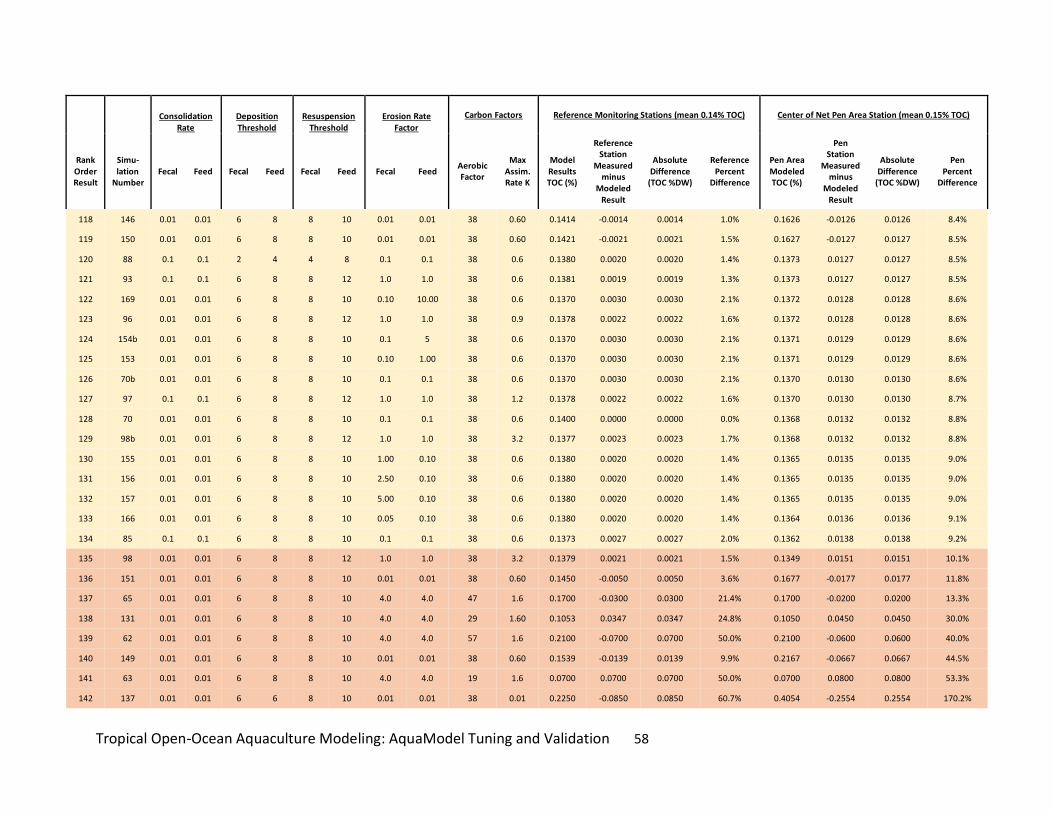
Tropical Open-Ocean Aquaculture Modeling: AquaModel Tuning and Validation 58
Consolidation
Rate Deposition Threshold
Resuspension Threshold
Erosion Rate Factor
Carbon Factors Reference Monitoring Stations (mean 0.14% TOC) Center of Net Pen Area Station (mean 0.15% TOC)
Rank Order Result
Simu-lation
Number Fecal Feed Fecal Feed Fecal Feed Fecal Feed
Aerobic Factor
Max Assim. Rate K
Model Results TOC (%)
Reference Station
Measured minus
Modeled Result
Absolute Difference
(TOC %DW)
Reference Percent
Difference
Pen Area Modeled TOC (%)
Pen Station
Measured minus
Modeled Result
Absolute Difference
(TOC %DW)
Pen Percent
Difference
118 146 0.01 0.01 6 8 8 10 0.01 0.01 38 0.60 0.1414 -0.0014 0.0014 1.0% 0.1626 -0.0126 0.0126 8.4%
119 150 0.01 0.01 6 8 8 10 0.01 0.01 38 0.60 0.1421 -0.0021 0.0021 1.5% 0.1627 -0.0127 0.0127 8.5%
120 88 0.1 0.1 2 4 4 8 0.1 0.1 38 0.6 0.1380 0.0020 0.0020 1.4% 0.1373 0.0127 0.0127 8.5%
121 93 0.1 0.1 6 8 8 12 1.0 1.0 38 0.6 0.1381 0.0019 0.0019 1.3% 0.1373 0.0127 0.0127 8.5%
122 169 0.01 0.01 6 8 8 10 0.10 10.00 38 0.6 0.1370 0.0030 0.0030 2.1% 0.1372 0.0128 0.0128 8.6%
123 96 0.01 0.01 6 8 8 12 1.0 1.0 38 0.9 0.1378 0.0022 0.0022 1.6% 0.1372 0.0128 0.0128 8.6%
124 154b 0.01 0.01 6 8 8 10 0.1 5 38 0.6 0.1370 0.0030 0.0030 2.1% 0.1371 0.0129 0.0129 8.6%
125 153 0.01 0.01 6 8 8 10 0.10 1.00 38 0.6 0.1370 0.0030 0.0030 2.1% 0.1371 0.0129 0.0129 8.6%
126 70b 0.01 0.01 6 8 8 10 0.1 0.1 38 0.6 0.1370 0.0030 0.0030 2.1% 0.1370 0.0130 0.0130 8.6%
127 97 0.1 0.1 6 8 8 12 1.0 1.0 38 1.2 0.1378 0.0022 0.0022 1.6% 0.1370 0.0130 0.0130 8.7%
128 70 0.01 0.01 6 8 8 10 0.1 0.1 38 0.6 0.1400 0.0000 0.0000 0.0% 0.1368 0.0132 0.0132 8.8%
129 98b 0.01 0.01 6 8 8 12 1.0 1.0 38 3.2 0.1377 0.0023 0.0023 1.7% 0.1368 0.0132 0.0132 8.8%
130 155 0.01 0.01 6 8 8 10 1.00 0.10 38 0.6 0.1380 0.0020 0.0020 1.4% 0.1365 0.0135 0.0135 9.0%
131 156 0.01 0.01 6 8 8 10 2.50 0.10 38 0.6 0.1380 0.0020 0.0020 1.4% 0.1365 0.0135 0.0135 9.0%
132 157 0.01 0.01 6 8 8 10 5.00 0.10 38 0.6 0.1380 0.0020 0.0020 1.4% 0.1365 0.0135 0.0135 9.0%
133 166 0.01 0.01 6 8 8 10 0.05 0.10 38 0.6 0.1380 0.0020 0.0020 1.4% 0.1364 0.0136 0.0136 9.1%
134 85 0.1 0.1 6 8 8 10 0.1 0.1 38 0.6 0.1373 0.0027 0.0027 2.0% 0.1362 0.0138 0.0138 9.2%
135 98 0.01 0.01 6 8 8 12 1.0 1.0 38 3.2 0.1379 0.0021 0.0021 1.5% 0.1349 0.0151 0.0151 10.1%
136 151 0.01 0.01 6 8 8 10 0.01 0.01 38 0.60 0.1450 -0.0050 0.0050 3.6% 0.1677 -0.0177 0.0177 11.8%
137 65 0.01 0.01 6 8 8 10 4.0 4.0 47 1.6 0.1700 -0.0300 0.0300 21.4% 0.1700 -0.0200 0.0200 13.3%
138 131 0.01 0.01 6 8 8 10 4.0 4.0 29 1.60 0.1053 0.0347 0.0347 24.8% 0.1050 0.0450 0.0450 30.0%
139 62 0.01 0.01 6 8 8 10 4.0 4.0 57 1.6 0.2100 -0.0700 0.0700 50.0% 0.2100 -0.0600 0.0600 40.0%
140 149 0.01 0.01 6 8 8 10 0.01 0.01 38 0.60 0.1539 -0.0139 0.0139 9.9% 0.2167 -0.0667 0.0667 44.5%
141 63 0.01 0.01 6 8 8 10 4.0 4.0 19 1.6 0.0700 0.0700 0.0700 50.0% 0.0700 0.0800 0.0800 53.3%
142 137 0.01 0.01 6 6 8 10 0.01 0.01 38 0.01 0.2250 -0.0850 0.0850 60.7% 0.4054 -0.2554 0.2554 170.2%
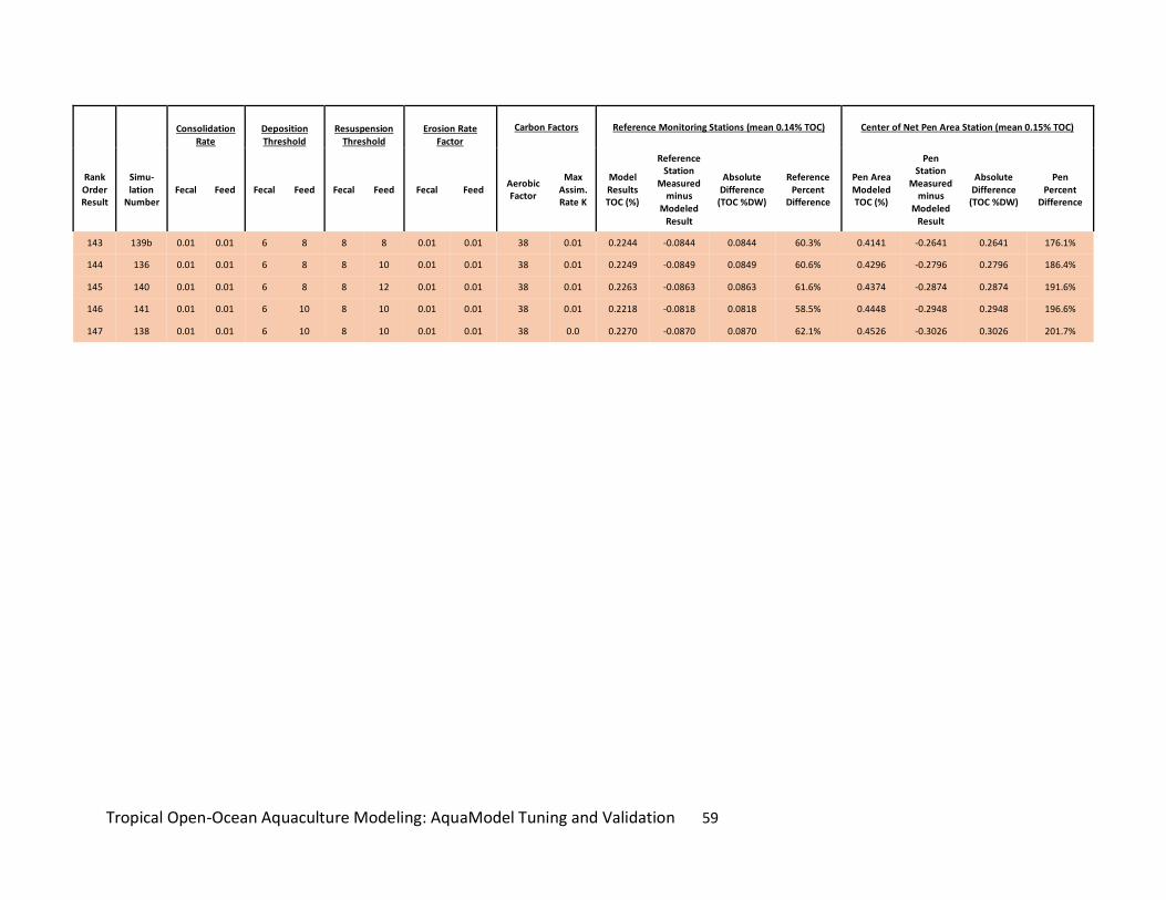
Tropical Open-Ocean Aquaculture Modeling: AquaModel Tuning and Validation 59
Consolidation
Rate Deposition Threshold
Resuspension Threshold
Erosion Rate Factor
Carbon Factors Reference Monitoring Stations (mean 0.14% TOC) Center of Net Pen Area Station (mean 0.15% TOC)
Rank Order Result
Simu-lation
Number Fecal Feed Fecal Feed Fecal Feed Fecal Feed
Aerobic Factor
Max Assim. Rate K
Model Results TOC (%)
Reference Station
Measured minus
Modeled Result
Absolute Difference
(TOC %DW)
Reference Percent
Difference
Pen Area Modeled TOC (%)
Pen Station
Measured minus
Modeled Result
Absolute Difference
(TOC %DW)
Pen Percent
Difference
143 139b 0.01 0.01 6 8 8 8 0.01 0.01 38 0.01 0.2244 -0.0844 0.0844 60.3% 0.4141 -0.2641 0.2641 176.1%
144 136 0.01 0.01 6 8 8 10 0.01 0.01 38 0.01 0.2249 -0.0849 0.0849 60.6% 0.4296 -0.2796 0.2796 186.4%
145 140 0.01 0.01 6 8 8 12 0.01 0.01 38 0.01 0.2263 -0.0863 0.0863 61.6% 0.4374 -0.2874 0.2874 191.6%
146 141 0.01 0.01 6 10 8 10 0.01 0.01 38 0.01 0.2218 -0.0818 0.0818 58.5% 0.4448 -0.2948 0.2948 196.6%
147 138 0.01 0.01 6 10 8 10 0.01 0.01 38 0.0 0.2270 -0.0870 0.0870 62.1% 0.4526 -0.3026 0.3026 201.7%

Tropical Open-Ocean Aquaculture Modeling: AquaModel Tuning and Validation 60
Appendix E. List of simulation settings assessed in later part of validation study and resulting skill of model to fit a mean of 0.16% sediment TOC at the center of lease area of Blue Ocean Mariculture.
Skill expressed as a) model predicted percent TOC; b) model vs mean observed difference, c) absolute difference of b and d) overall percent difference. Total N = 210. Colored background groups different classes of optimum fit between modeled and observed results.
Consolidation
Rate Deposition Threshold
Resuspenion Threshold
Erosion Rate Factor
Carbon Factors Reference Monitoring Stations
mean 0.14% TOC Center of Net Pen Area Station
mean 0.16% TOC
Rank Order Result
Simu-lation
Number Fecal Feed Fecal Feed Fecal Feed Fecal Feed
Aerobic factor
Max Assim. Rate k
Model Results TOC (%)
Reference Station
Measured minus
Modeled Result
Absolute Difference
(TOC %DW)
Reference Percent
Difference
Pen Area Modeled TOC (%)
Pen Station
Measured minus
Modeled Result
Absolute Difference
(TOC %DW)
Pen Percent
Difference
1 143 0.01 0.01 6 8 8 10 0.01 0.01 38 0.60 0.1489 -0.0089 0.0089 6.3% 0.1620 -0.0020 0.0020 1.3%
2 143b 0.01 0.01 6 8 8 10 0.01 0.01 38 0.60 0.1489 -0.0089 0.0089 6.3% 0.1620 -0.0020 0.0020 1.3%
3 128 0.01 0.01 6 10 8 16 0.01 0.01 38 0.30 0.1430 -0.0030 0.0030 2.2% 0.1579 0.0021 0.0021 1.3%
4 146 0.01 0.01 6 8 8 10 0.01 0.01 38 0.60 0.1414 -0.0014 0.0014 1.0% 0.1626 -0.0026 0.0026 1.6%
5 150 0.01 0.01 6 8 8 10 0.01 0.01 38 0.60 0.1421 -0.0021 0.0021 1.5% 0.1627 -0.0027 0.0027 1.7%
6 92 0.1 0.1 8 10 10 16 0.1 0.1 38 0.3 0.1404 -0.0004 0.0004 0.3% 0.1542 0.0058 0.0058 3.6%
7 113 0.1 0.1 8 10 10 16 0.1 0.1 38 0.3 0.1378 0.0022 0.0022 1.6% 0.1540 0.0060 0.0060 3.8%
8 114 0.01 0.01 8 10 10 16 0.1 0.1 38 0.3 0.1378 0.0022 0.0022 1.6% 0.1540 0.0060 0.0060 3.8%
9 151 0.01 0.01 6 8 8 10 0.01 0.01 38 0.60 0.1450 -0.0050 0.0050 3.6% 0.1677 -0.0077 0.0077 4.8%
10 129 0.01 0.01 6 8 8 14 0.01 0.01 38 0.30 0.1412 -0.0012 0.0012 0.8% 0.1518 0.0082 0.0082 5.1%
11 127 0.01 0.01 6 8 8 10 0.01 0.01 38 0.50 0.1411 -0.0011 0.0011 0.8% 0.1516 0.0084 0.0084 5.2%
12 174 0.01 0.01 6 8 8 10 0.001 0.001 38 0.6 0.1415 -0.0015 0.0015 1.1% 0.1508 0.0092 0.0092 5.8%
13 198 10 10 6 8 8 10 0.01 0.01 38 0.6 0.1413 -0.0013 0.0013 0.9% 0.1507 0.0093 0.0093 5.8%
14 180b 0.01 0.01 6 8 8 10 0.001 0.01 38 0.6 0.1413 -0.0013 0.0013 0.9% 0.1506 0.0094 0.0094 5.9%
15 133 0.01 0.01 6 10 8 10 0.01 0.01 38 0.60 0.1406 -0.0006 0.0006 0.4% 0.1506 0.0094 0.0094 5.9%
16 170 0.01 0.01 6 8 8 10 0.010 0.001 38 0.6 0.1411 -0.0011 0.0011 0.8% 0.1504 0.0096 0.0096 6.0%
17 186b 0.01 0.01 6 8 8 10 0.01 0.001 38 0.6 0.1411 -0.0011 0.0011 0.8% 0.1504 0.0096 0.0096 6.0%
18 135 0.01 0.01 6 8 8 12 0.01 0.01 38 0.60 0.1407 -0.0007 0.0007 0.5% 0.1501 0.0099 0.0099 6.2%
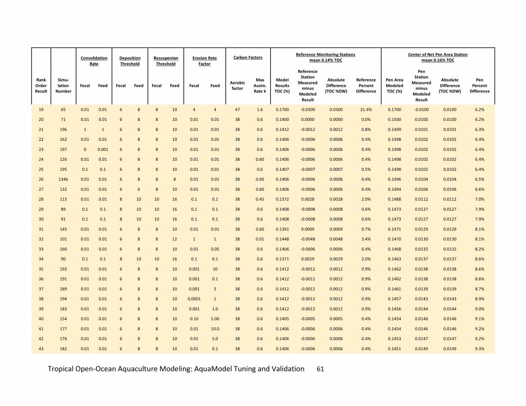
Tropical Open-Ocean Aquaculture Modeling: AquaModel Tuning and Validation 61
Consolidation
Rate Deposition Threshold
Resuspenion Threshold
Erosion Rate Factor
Carbon Factors Reference Monitoring Stations
mean 0.14% TOC Center of Net Pen Area Station
mean 0.16% TOC
Rank Order Result
Simu-lation
Number Fecal Feed Fecal Feed Fecal Feed Fecal Feed
Aerobic factor
Max Assim. Rate k
Model Results TOC (%)
Reference Station
Measured minus
Modeled Result
Absolute Difference
(TOC %DW)
Reference Percent
Difference
Pen Area Modeled TOC (%)
Pen Station
Measured minus
Modeled Result
Absolute Difference
(TOC %DW)
Pen Percent
Difference
19 65 0.01 0.01 6 8 8 10 4 4 47 1.6 0.1700 -0.0300 0.0300 21.4% 0.1700 -0.0100 0.0100 6.2%
20 71 0.01 0.01 6 8 8 10 0.01 0.01 38 0.6 0.1400 0.0000 0.0000 0.0% 0.1500 0.0100 0.0100 6.2%
21 196 1 1 6 8 8 10 0.01 0.01 38 0.6 0.1412 -0.0012 0.0012 0.8% 0.1499 0.0101 0.0101 6.3%
22 162 0.01 0.01 6 8 8 10 0.01 0.01 38 0.6 0.1406 -0.0006 0.0006 0.4% 0.1498 0.0102 0.0102 6.4%
23 197 0 0.001 6 8 8 10 0.01 0.01 38 0.6 0.1406 -0.0006 0.0006 0.4% 0.1498 0.0102 0.0102 6.4%
24 126 0.01 0.01 6 8 8 10 0.01 0.01 38 0.60 0.1406 -0.0006 0.0006 0.4% 0.1498 0.0102 0.0102 6.4%
25 195 0.1 0.1 6 8 8 10 0.01 0.01 38 0.6 0.1407 -0.0007 0.0007 0.5% 0.1498 0.0102 0.0102 6.4%
26 134b 0.01 0.01 6 8 8 8 0.01 0.01 38 0.60 0.1406 -0.0006 0.0006 0.4% 0.1496 0.0104 0.0104 6.5%
27 132 0.01 0.01 6 6 8 10 0.01 0.01 38 0.60 0.1406 -0.0006 0.0006 0.4% 0.1494 0.0106 0.0106 6.6%
28 115 0.01 0.01 8 10 10 16 0.1 0.1 38 0.45 0.1372 0.0028 0.0028 2.0% 0.1488 0.0112 0.0112 7.0%
29 89 0.1 0.1 8 10 10 16 0.1 0.1 38 0.6 0.1408 -0.0008 0.0008 0.6% 0.1473 0.0127 0.0127 7.9%
30 91 0.1 0.1 8 10 10 16 0.1 0.1 38 0.6 0.1408 -0.0008 0.0008 0.6% 0.1473 0.0127 0.0127 7.9%
31 145 0.01 0.01 6 8 8 10 0.01 0.01 38 0.60 0.1391 0.0009 0.0009 0.7% 0.1471 0.0129 0.0129 8.1%
32 101 0.01 0.01 6 8 8 12 1 1 38 0.01 0.1448 -0.0048 0.0048 3.4% 0.1470 0.0130 0.0130 8.1%
33 160 0.01 0.01 6 8 8 10 0.01 0.05 38 0.6 0.1406 -0.0006 0.0006 0.4% 0.1468 0.0132 0.0132 8.2%
34 90 0.1 0.1 8 10 10 16 0.1 0.1 38 0.6 0.1371 0.0029 0.0029 2.0% 0.1463 0.0137 0.0137 8.6%
35 192 0.01 0.01 6 8 8 10 0.001 10 38 0.6 0.1412 -0.0012 0.0012 0.9% 0.1462 0.0138 0.0138 8.6%
36 191 0.01 0.01 6 8 8 10 0.001 0.1 38 0.6 0.1412 -0.0012 0.0012 0.9% 0.1462 0.0138 0.0138 8.6%
37 189 0.01 0.01 6 8 8 10 0.001 5 38 0.6 0.1412 -0.0012 0.0012 0.9% 0.1461 0.0139 0.0139 8.7%
38 194 0.01 0.01 6 8 8 10 0.0001 1 38 0.6 0.1412 -0.0012 0.0012 0.9% 0.1457 0.0143 0.0143 8.9%
39 183 0.01 0.01 6 8 8 10 0.001 1.0 38 0.6 0.1412 -0.0012 0.0012 0.9% 0.1456 0.0144 0.0144 9.0%
40 154 0.01 0.01 6 8 8 10 0.10 5.00 38 0.6 0.1405 -0.0005 0.0005 0.4% 0.1454 0.0146 0.0146 9.1%
41 177 0.01 0.01 6 8 8 10 0.01 10.0 38 0.6 0.1406 -0.0006 0.0006 0.4% 0.1454 0.0146 0.0146 9.2%
42 176 0.01 0.01 6 8 8 10 0.01 5.0 38 0.6 0.1406 -0.0006 0.0006 0.4% 0.1453 0.0147 0.0147 9.2%
43 182 0.01 0.01 6 8 8 10 0.01 0.1 38 0.6 0.1406 -0.0006 0.0006 0.4% 0.1451 0.0149 0.0149 9.3%
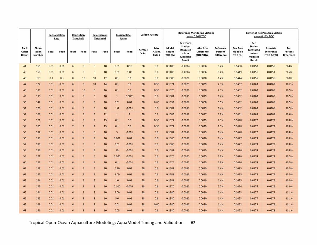
Tropical Open-Ocean Aquaculture Modeling: AquaModel Tuning and Validation 62
Consolidation
Rate Deposition Threshold
Resuspenion Threshold
Erosion Rate Factor
Carbon Factors Reference Monitoring Stations
mean 0.14% TOC Center of Net Pen Area Station
mean 0.16% TOC
Rank Order Result
Simu-lation
Number Fecal Feed Fecal Feed Fecal Feed Fecal Feed
Aerobic factor
Max Assim. Rate k
Model Results TOC (%)
Reference Station
Measured minus
Modeled Result
Absolute Difference
(TOC %DW)
Reference Percent
Difference
Pen Area Modeled TOC (%)
Pen Station
Measured minus
Modeled Result
Absolute Difference
(TOC %DW)
Pen Percent
Difference
44 165 0.01 0.01 6 8 8 10 0.01 0.10 38 0.6 0.1406 -0.0006 0.0006 0.4% 0.1450 0.0150 0.0150 9.4%
45 158 0.01 0.01 6 8 8 10 0.01 1.00 38 0.6 0.1406 -0.0006 0.0006 0.4% 0.1449 0.0151 0.0151 9.5%
46 87 0.1 0.1 8 10 10 12 0.1 0.1 38 0.6 0.1380 0.0020 0.0020 1.4% 0.1444 0.0156 0.0156 9.8%
47 122 0.01 0.01 6 8 10 14 0.1 0.1 38 0.50 0.1371 0.0029 0.0029 2.1% 0.1437 0.0163 0.0163 10.2%
48 130 0.01 0.01 6 10 8 16 0.1 0.1 38 0.50 0.1370 0.0030 0.0030 2.1% 0.1432 0.0168 0.0168 10.5%
49 193 0.01 0.01 6 8 8 10 1 0.0001 38 0.6 0.1381 0.0019 0.0019 1.4% 0.1432 0.0168 0.0168 10.5%
50 142 0.01 0.01 6 8 8 10 0.01 0.01 38 0.60 0.1392 0.0008 0.0008 0.5% 0.1432 0.0168 0.0168 10.5%
51 178 0.01 0.01 6 8 8 10 1.0 0.001 38 0.6 0.1381 0.0019 0.0019 1.4% 0.1432 0.0168 0.0168 10.5%
52 108 0.01 0.01 6 8 8 12 1 1 38 0.1 0.1383 0.0017 0.0017 1.2% 0.1431 0.0169 0.0169 10.6%
53 121 0.01 0.01 6 8 9 13 0.1 0.1 38 0.50 0.1371 0.0029 0.0029 2.1% 0.1428 0.0172 0.0172 10.8%
54 125 0.01 0.01 7 9 9 13 0.1 0.1 38 0.50 0.1371 0.0029 0.0029 2.1% 0.1428 0.0172 0.0172 10.8%
55 187 0.01 0.01 6 8 8 10 5 0.001 38 0.6 0.1381 0.0019 0.0019 1.4% 0.1428 0.0172 0.0172 10.8%
56 180 0.01 0.01 6 8 8 10 0.001 0.01 38 0.6 0.1380 0.0020 0.0020 1.4% 0.1427 0.0173 0.0173 10.8%
57 186 0.01 0.01 6 8 8 10 0.01 0.001 38 0.6 0.1380 0.0020 0.0020 1.4% 0.1427 0.0173 0.0173 10.8%
58 188 0.01 0.01 6 8 8 10 10 0.001 38 0.6 0.1381 0.0019 0.0019 1.4% 0.1426 0.0174 0.0174 10.8%
59 171 0.01 0.01 6 8 8 10 0.100 0.001 38 0.6 0.1375 0.0025 0.0025 1.8% 0.1426 0.0174 0.0174 10.9%
60 181 0.01 0.01 6 8 8 10 0.1 0.001 38 0.6 0.1375 0.0025 0.0025 1.8% 0.1426 0.0174 0.0174 10.9%
61 152 0.01 0.01 6 8 8 10 0.10 0.01 38 0.6 0.1381 0.0019 0.0019 1.4% 0.1425 0.0175 0.0175 10.9%
62 163 0.01 0.01 6 8 8 10 1.00 0.01 38 0.6 0.1381 0.0019 0.0019 1.4% 0.1425 0.0175 0.0175 10.9%
63 184 0.01 0.01 6 8 8 10 1.0 0.01 38 0.6 0.1381 0.0019 0.0019 1.4% 0.1425 0.0175 0.0175 10.9%
64 172 0.01 0.01 6 8 8 10 0.100 0.005 38 0.6 0.1370 0.0030 0.0030 2.2% 0.1424 0.0176 0.0176 11.0%
65 164 0.01 0.01 6 8 8 10 5.00 0.01 38 0.6 0.1380 0.0020 0.0020 1.4% 0.1423 0.0177 0.0177 11.1%
66 185 0.01 0.01 6 8 8 10 5.0 0.01 38 0.6 0.1380 0.0020 0.0020 1.4% 0.1423 0.0177 0.0177 11.1%
67 148 0.01 0.01 6 8 8 10 0.01 0.01 38 0.60 0.1380 0.0020 0.0020 1.4% 0.1422 0.0178 0.0178 11.1%
68 161 0.01 0.01 6 8 8 10 0.05 0.01 38 0.6 0.1380 0.0020 0.0020 1.4% 0.1422 0.0178 0.0178 11.1%
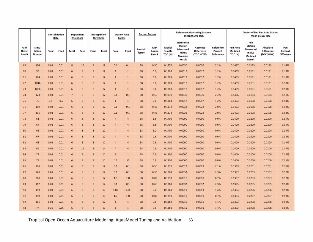
Tropical Open-Ocean Aquaculture Modeling: AquaModel Tuning and Validation 63
Consolidation
Rate Deposition Threshold
Resuspenion Threshold
Erosion Rate Factor
Carbon Factors Reference Monitoring Stations
mean 0.14% TOC Center of Net Pen Area Station
mean 0.16% TOC
Rank Order Result
Simu-lation
Number Fecal Feed Fecal Feed Fecal Feed Fecal Feed
Aerobic factor
Max Assim. Rate k
Model Results TOC (%)
Reference Station
Measured minus
Modeled Result
Absolute Difference
(TOC %DW)
Reference Percent
Difference
Pen Area Modeled TOC (%)
Pen Station
Measured minus
Modeled Result
Absolute Difference
(TOC %DW)
Pen Percent
Difference
69 124 0.01 0.01 8 10 8 12 0.1 0.1 38 0.50 0.1370 0.0030 0.0030 2.2% 0.1417 0.0183 0.0183 11.4%
70 95 0.01 0.01 6 8 8 12 1 1 38 0.1 0.1383 0.0017 0.0017 1.2% 0.1409 0.0191 0.0191 11.9%
71 104 0.01 0.01 6 8 8 12 1 1 38 0.1 0.1383 0.0017 0.0017 1.2% 0.1409 0.0191 0.0191 11.9%
72 104b 0.01 0.01 6 8 8 12 1 1 38 0.1 0.1383 0.0017 0.0017 1.2% 0.1409 0.0191 0.0191 12.0%
73 108b 0.01 0.01 6 8 8 12 1 1 38 0.1 0.1383 0.0017 0.0017 1.2% 0.1409 0.0191 0.0191 12.0%
74 123 0.01 0.01 7 9 8 12 0.1 0.1 38 0.50 0.1370 0.0030 0.0030 2.2% 0.1406 0.0194 0.0194 12.1%
75 76 0.5 0.5 6 8 8 10 1 1 38 0.6 0.1383 0.0017 0.0017 1.2% 0.1402 0.0198 0.0198 12.4%
76 119 0.01 0.01 6 8 8 12 0.1 0.1 38 0.45 0.1372 0.0028 0.0028 2.0% 0.1402 0.0198 0.0198 12.4%
77 116 0.01 0.01 6 8 8 12 0.1 0.1 38 0.45 0.1372 0.0028 0.0028 2.0% 0.1402 0.0198 0.0198 12.4%
78 61 0.01 0.01 6 8 8 10 4 4 38 1.6 0.1400 0.0000 0.0000 0.0% 0.1400 0.0200 0.0200 12.5%
79 64 0.01 0.01 6 8 8 10 4 4 38 1.6 0.1400 0.0000 0.0000 0.0% 0.1400 0.0200 0.0200 12.5%
80 66 0.01 0.01 6 8 8 10 4 4 38 3.2 0.1400 0.0000 0.0000 0.0% 0.1400 0.0200 0.0200 12.5%
81 67 0.01 0.01 6 8 8 10 4 4 38 0.6 0.1400 0.0000 0.0000 0.0% 0.1400 0.0200 0.0200 12.5%
82 68 0.01 0.01 6 8 8 10 4 4 38 0.6 0.1400 0.0000 0.0000 0.0% 0.1400 0.0200 0.0200 12.5%
83 69 0.01 0.01 6 12 8 14 4 4 38 0.6 0.1400 0.0000 0.0000 0.0% 0.1400 0.0200 0.0200 12.5%
84 72 0.01 0.01 6 8 8 10 1 1 38 0.6 0.1400 0.0000 0.0000 0.0% 0.1400 0.0200 0.0200 12.5%
85 73 0.01 0.01 6 8 8 10 10 10 38 0.6 0.1400 0.0000 0.0000 0.0% 0.1400 0.0200 0.0200 12.5%
86 118 0.01 0.01 6 8 8 12 0.1 0.1 38 0.50 0.1371 0.0029 0.0029 2.1% 0.1399 0.0201 0.0201 12.6%
87 120 0.01 0.01 6 8 8 12 0.1 0.1 38 0.55 0.1368 0.0032 0.0032 2.3% 0.1397 0.0203 0.0203 12.7%
88 200 0.01 0.01 6 8 8 12 1.0 1.0 38 0.05 0.1390 0.0010 0.0010 0.7% 0.1397 0.0203 0.0203 12.7%
89 117 0.01 0.01 6 8 8 12 0.1 0.1 38 0.60 0.1368 0.0032 0.0032 2.3% 0.1395 0.0205 0.0205 12.8%
90 159 0.01 0.01 6 8 8 10 1.00 0.05 38 0.6 0.1381 0.0019 0.0019 1.4% 0.1394 0.0206 0.0206 12.9%
91 199 0.01 0.01 6 8 8 10 1.0 1.0 38 0.05 0.1390 0.0010 0.0010 0.7% 0.1393 0.0207 0.0207 12.9%
92 111 0.01 0.01 6 8 8 12 1 1 38 0.1 0.1384 0.0016 0.0016 1.1% 0.1392 0.0208 0.0208 13.0%
93 77 0.25 0.25 6 8 8 10 1 1 38 0.6 0.1381 0.0019 0.0019 1.4% 0.1392 0.0208 0.0208 13.0%

Tropical Open-Ocean Aquaculture Modeling: AquaModel Tuning and Validation 64
Consolidation
Rate Deposition Threshold
Resuspenion Threshold
Erosion Rate Factor
Carbon Factors Reference Monitoring Stations
mean 0.14% TOC Center of Net Pen Area Station
mean 0.16% TOC
Rank Order Result
Simu-lation
Number Fecal Feed Fecal Feed Fecal Feed Fecal Feed
Aerobic factor
Max Assim. Rate k
Model Results TOC (%)
Reference Station
Measured minus
Modeled Result
Absolute Difference
(TOC %DW)
Reference Percent
Difference
Pen Area Modeled TOC (%)
Pen Station
Measured minus
Modeled Result
Absolute Difference
(TOC %DW)
Pen Percent
Difference
94 112 0.01 0.01 6 8 8 12 1 1 38 0.1 0.1385 0.0015 0.0015 1.1% 0.1391 0.0209 0.0209 13.0%
95 107 0.01 0.01 6 8 8 12 1 1 38 0.1 0.1385 0.0015 0.0015 1.1% 0.1391 0.0209 0.0209 13.0%
96 109 0.01 0.01 6 8 8 12 1 1 38 0.1 0.1385 0.0015 0.0015 1.1% 0.1391 0.0209 0.0209 13.0%
97 110 0.01 0.01 6 8 8 12 1 1 38 0.1 0.1385 0.0015 0.0015 1.1% 0.1391 0.0209 0.0209 13.0%
98 95b 0.01 0.01 6 8 8 12 1 1 38 0.1 0.1385 0.0015 0.0015 1.1% 0.1391 0.0209 0.0209 13.0%
99 99 0.01 0.01 6 8 8 12 1 1 38 0.1 0.1386 0.0014 0.0014 1.0% 0.1391 0.0209 0.0209 13.1%
100 100 0.01 0.01 6 8 8 12 1 1 38 0.1 0.1386 0.0014 0.0014 1.0% 0.1391 0.0209 0.0209 13.1%
101 95switch 0.01 0.01 6 8 8 12 1 1 38 0.1 0.1386 0.0014 0.0014 1.0% 0.1391 0.0209 0.0209 13.1%
102 102 0.01 0.01 6 8 8 12 1 1 38 0.1 0.1386 0.0014 0.0014 1.0% 0.1391 0.0209 0.0209 13.1%
103 103 0.01 0.01 6 8 8 12 1 1 38 0.1 0.1388 0.0012 0.0012 0.9% 0.1390 0.0210 0.0210 13.1%
104 106 0.01 0.01 6 8 8 12 1 1 38 0.1 0.1388 0.0012 0.0012 0.9% 0.1390 0.0210 0.0210 13.1%
105 99switch 0.01 0.01 6 8 8 12 1 1 38 0.1 0.1388 0.0012 0.0012 0.9% 0.1390 0.0210 0.0210 13.1%
106 78 0.1 0.1 6 8 8 10 1 1 38 0.6 0.1381 0.0019 0.0019 1.4% 0.1383 0.0217 0.0217 13.6%
107 79 0.1 0.1 6 8 8 10 1 1 38 0.6 0.1381 0.0019 0.0019 1.4% 0.1383 0.0217 0.0217 13.6%
108 83 0.1 0.1 6 8 8 10 1 1 38 0.6 0.1381 0.0019 0.0019 1.4% 0.1383 0.0217 0.0217 13.6%
109 82 0.1 0.1 6 8 8 10 2 2 38 0.6 0.1381 0.0019 0.0019 1.4% 0.1382 0.0218 0.0218 13.6%
110 86 0.1 0.1 4 6 6 10 0.1 0.1 38 0.6 0.1381 0.0019 0.0019 1.4% 0.1382 0.0218 0.0218 13.6%
111 80 0.1 0.1 6 8 8 10 4 4 38 0.6 0.1381 0.0019 0.0019 1.4% 0.1382 0.0218 0.0218 13.6%
112 81 0.1 0.1 6 8 8 10 60.4 60.4 38 0.6 0.1380 0.0020 0.0020 1.4% 0.1381 0.0219 0.0219 13.7%
113 179 0.01 0.01 6 8 8 10 1.0 10.0 38 0.6 0.1380 0.0020 0.0020 1.4% 0.1380 0.0220 0.0220 13.7%
114 75 0.01 0.01 6 8 8 10 5 5 38 0.6 0.1380 0.0020 0.0020 1.4% 0.1378 0.0222 0.0222 13.8%
115 190 0.01 0.01 6 8 8 10 5 5 38 0.6 0.1380 0.0020 0.0020 1.4% 0.1378 0.0222 0.0222 13.9%
116 94 0.01 0.01 6 8 8 12 1 1 38 0.3 0.1381 0.0019 0.0019 1.4% 0.1377 0.0223 0.0223 13.9%
117 179b 0.01 0.01 6 8 8 10 1.0 10 38 0.6 0.1380 0.0020 0.0020 1.4% 0.1376 0.0224 0.0224 14.0%
118 168 0.01 0.01 6 8 8 10 1.00 5.00 38 0.6 0.1380 0.0020 0.0020 1.4% 0.1376 0.0224 0.0224 14.0%

Tropical Open-Ocean Aquaculture Modeling: AquaModel Tuning and Validation 65
Consolidation
Rate Deposition Threshold
Resuspenion Threshold
Erosion Rate Factor
Carbon Factors Reference Monitoring Stations
mean 0.14% TOC Center of Net Pen Area Station
mean 0.16% TOC
Rank Order Result
Simu-lation
Number Fecal Feed Fecal Feed Fecal Feed Fecal Feed
Aerobic factor
Max Assim. Rate k
Model Results TOC (%)
Reference Station
Measured minus
Modeled Result
Absolute Difference
(TOC %DW)
Reference Percent
Difference
Pen Area Modeled TOC (%)
Pen Station
Measured minus
Modeled Result
Absolute Difference
(TOC %DW)
Pen Percent
Difference
119 74 0.01 0.01 6 8 8 10 1 1 38 0.6 0.1381 0.0019 0.0019 1.4% 0.1374 0.0226 0.0226 14.1%
120 84 0.01 0.01 6 8 8 10 1 1 38 0.6 0.1381 0.0019 0.0019 1.4% 0.1374 0.0226 0.0226 14.1%
121 167 0.01 0.01 6 8 8 10 5.00 1.00 38 0.6 0.1380 0.0020 0.0020 1.4% 0.1374 0.0226 0.0226 14.1%
122 88 0.1 0.1 2 4 4 8 0.1 0.1 38 0.6 0.1380 0.0020 0.0020 1.4% 0.1373 0.0227 0.0227 14.2%
123 93 0.1 0.1 6 8 8 12 1 1 38 0.6 0.1381 0.0019 0.0019 1.3% 0.1373 0.0227 0.0227 14.2%
124 169 0.01 0.01 6 8 8 10 0.10 10.00 38 0.6 0.1370 0.0030 0.0030 2.1% 0.1372 0.0228 0.0228 14.3%
125 96 0.01 0.01 6 8 8 12 1 1 38 0.9 0.1378 0.0022 0.0022 1.6% 0.1372 0.0228 0.0228 14.3%
126 154b 0.01 0.01 6 8 8 10 0.1 5 38 0.6 0.1370 0.0030 0.0030 2.1% 0.1371 0.0229 0.0229 14.3%
127 153 0.01 0.01 6 8 8 10 0.10 1.00 38 0.6 0.1370 0.0030 0.0030 2.1% 0.1371 0.0229 0.0229 14.3%
128 70b 0.01 0.01 6 8 8 10 0.1 0.1 38 0.6 0.1370 0.0030 0.0030 2.1% 0.1370 0.0230 0.0230 14.4%
129 97 0.1 0.1 6 8 8 12 1 1 38 1.2 0.1378 0.0022 0.0022 1.6% 0.1370 0.0230 0.0230 14.4%
130 70 0.01 0.01 6 8 8 10 0.1 0.1 38 0.6 0.1400 0.0000 0.0000 0.0% 0.1368 0.0232 0.0232 14.5%
131 98b 0.01 0.01 6 8 8 12 1 1 38 3.2 0.1377 0.0023 0.0023 1.7% 0.1368 0.0232 0.0232 14.5%
132 155 0.01 0.01 6 8 8 10 1.00 0.10 38 0.6 0.1380 0.0020 0.0020 1.4% 0.1365 0.0235 0.0235 14.7%
133 156 0.01 0.01 6 8 8 10 2.50 0.10 38 0.6 0.1380 0.0020 0.0020 1.4% 0.1365 0.0235 0.0235 14.7%
134 157 0.01 0.01 6 8 8 10 5.00 0.10 38 0.6 0.1380 0.0020 0.0020 1.4% 0.1365 0.0235 0.0235 14.7%
135 166 0.01 0.01 6 8 8 10 0.05 0.10 38 0.6 0.1380 0.0020 0.0020 1.4% 0.1364 0.0236 0.0236 14.8%
136 85 0.1 0.1 6 8 8 10 0.1 0.1 38 0.6 0.1373 0.0027 0.0027 2.0% 0.1362 0.0238 0.0238 14.9%
137 98 0.01 0.01 6 8 8 12 1 1 38 3.2 0.1379 0.0021 0.0021 1.5% 0.1349 0.0251 0.0251 15.7%
138 62 0.01 0.01 6 8 8 10 4 4 57 1.6 0.2100 -0.0700 0.0700 50.0% 0.2100 -0.0500 0.0500 31.3%
139 131 0.01 0.01 6 8 8 10 4 4 29 1.60 0.1053 0.0347 0.0347 24.8% 0.1050 0.0550 0.0550 34.4%
140 149 0.01 0.01 6 8 8 10 0.01 0.01 38 0.60 0.1539 -0.0139 0.0139 9.9% 0.2167 -0.0567 0.0567 35.4%
141 63 0.01 0.01 6 8 8 10 4 4 19 1.6 0.0700 0.0700 0.0700 50.0% 0.0700 0.0900 0.0900 56.2%
142 137 0.01 0.01 6 6 8 10 0.01 0.01 38 0.01 0.2250 -0.0850 0.0850 60.7% 0.4054 -0.2454 0.2454 153.4%
143 139b 0.01 0.01 6 8 8 8 0.01 0.01 38 0.01 0.2244 -0.0844 0.0844 60.3% 0.4141 -0.2541 0.2541 158.8%
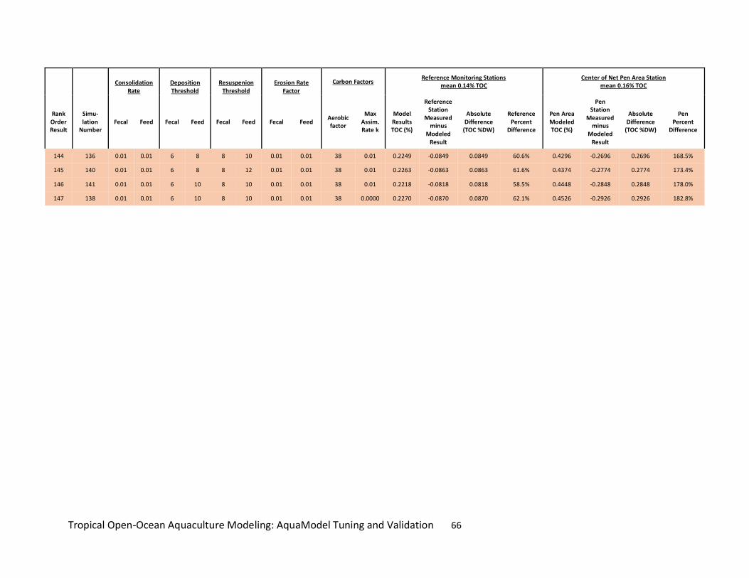
Tropical Open-Ocean Aquaculture Modeling: AquaModel Tuning and Validation 66
Consolidation
Rate Deposition Threshold
Resuspenion Threshold
Erosion Rate Factor
Carbon Factors Reference Monitoring Stations
mean 0.14% TOC Center of Net Pen Area Station
mean 0.16% TOC
Rank Order Result
Simu-lation
Number Fecal Feed Fecal Feed Fecal Feed Fecal Feed
Aerobic factor
Max Assim. Rate k
Model Results TOC (%)
Reference Station
Measured minus
Modeled Result
Absolute Difference
(TOC %DW)
Reference Percent
Difference
Pen Area Modeled TOC (%)
Pen Station
Measured minus
Modeled Result
Absolute Difference
(TOC %DW)
Pen Percent
Difference
144 136 0.01 0.01 6 8 8 10 0.01 0.01 38 0.01 0.2249 -0.0849 0.0849 60.6% 0.4296 -0.2696 0.2696 168.5%
145 140 0.01 0.01 6 8 8 12 0.01 0.01 38 0.01 0.2263 -0.0863 0.0863 61.6% 0.4374 -0.2774 0.2774 173.4%
146 141 0.01 0.01 6 10 8 10 0.01 0.01 38 0.01 0.2218 -0.0818 0.0818 58.5% 0.4448 -0.2848 0.2848 178.0%
147 138 0.01 0.01 6 10 8 10 0.01 0.01 38 0.0000 0.2270 -0.0870 0.0870 62.1% 0.4526 -0.2926 0.2926 182.8%