TROPICAL GEOMETRY TO ANALYSEDEMAND

Elizabeth Baldwin∗ and Paul Klemperer†

preliminary draft May 2012;this July 2014 draft is a minor revision of the October, 2013 version;

a significant revision is in progress

The latest version of this paper and related material will be athttp://users.ox.ac.uk/∼wadh1180/ and www.paulklemperer.org

ABSTRACT

Duality techniques from convex geometry, extended by the recently-developed math-ematics of tropical geometry, provide a powerful lens to study demand. We propose anew framework of “demand types”, for categorising and understanding demand; ourclassification both incorporates existing definitions (such as substitutes, complements,“strong substitutes”, etc.) and permits additional distinctions. We obtain easy-to-checknecessary and sufficient conditions for the existence of a competitive equilibrium for in-divisible goods. Our techniques also underpin Klemperer’s (2008) Product-Mix Auction,introduced by the Bank of England in the financial crisis.

JEL nos: C62 Existence and Stability Conditions of Equilibrium; D50 General Equilibrium

and Disequilibrium; D44 Auctions

Keywords: equilibrium existence; general equilibrium; competitive equilibrium; duality;

indivisible goods; tropical geometry; convex geometry; product mix auction; product-mix

auction; auction; strong substitute; substitute; complement; gross substitute; weak substitute

Acknowledgements: to be completed later

∗Grantham Research Institute, London School of Economics, UK. e.c.baldwin@lse.ac.uk†Nuffield College, Oxford University, UK. paul.klemperer@economics.ox.ac.uk

1

1 Introduction

This paper introduces a new way to think about economic agents’ individual andaggregate demands for indivisible goods,1 and provides a new set of geometric toolsto use for this. Our model applies to agents who buy and/or sell, as well as to somematching models.

Economists mostly think about agents’ demands by focusing on the direct utilityfunctions. We instead begin by focusing on the geometric structure of the regions ofprice space in which an agent demands different bundles. Our crucial observation isthat dividing price space in this way creates precisely the geometric structure which isstudied in the recently-developed, non-Euclidean, branch of algebraic geometry called“tropical geometry”.2 We can therefore use the tools of convex and tropical geometry,such as the duality between the geometric structure of an agent’s demand in price spaceand the same agent’s demand in quantity space, to obtain new insights about demand.Moving backwards and forwards between the dual representations of demand in pricespace and quantity space improves our understanding of both.

For example, it is much easier to aggregate individual demands in price space, buttranslating aggregate demand back into quantity space allows a strong theorem thatencompasses and extends many existing results about when a competitive equilibriumexists.

On the other hand, if we start from the (direct) valuation function in quantityspace, our methods for translating to the dual in price space quickly reveal the keyproperties of demand. Many existing results in demand theory can be understood morereadily, and developed more efficiently, using our tropical-geometric perspective thanusing traditional methods.

Individual demandExamining these geometric structures also suggests a natural way of classifying de-

mand: we say two valuations have the same “type” if certain sets of vectors associatedwith the geometric structures are the same.

Importantly, “types” are not merely a mathematically convenient way to categorisedemands. The list of vectors in the demand type is a list of possible ways an agent’sdemand can change when prices change. So it specifies the possible comparative statics ofdemand, and thus much of what economists think important about valuations. Familiarconcepts such as substitutes and complements are examples of “types”.

For example, a purchaser of new spectacles who is interested in having spare pairsmight always buy lenses and frames in the ratio 2:1, whatever the individual prices ofthe goods. So when running an auction in which goods’ characteristics suggest natural

1Baldwin and Klemperer (in preparation) show the relevance of our techniques to analysing divisiblegoods also, in contexts such as the Product-Mix Auction.

2This assumes, as is standard in the indivisible-goods literature, that preferences are quasilinear.Tropical geometry was developed by, among others, Mikhalkin (2004, 2005). We believe it has notpreviously been applied to economics. Goeree and Kushnir (2012) have recently used techniques ofconvex analysis (see, e.g., Rockafellar, 1970), on which tropical geometry builds, in a very differentcontext. However, Danilov and Koshevoy, with their coauthors (see, in particular, Danilov et al., 2001,Danilov et al., 2003 and Danilov and Koshevoy, 2004) have developed methods of discrete convexanalysis with closer connections to ours which we discuss later in the Introduction, and in detail inSections 4 and 6.3.

2

rates of substitution, bidders can be asked to express preferences that come from thecorresponding demand type.3

Our classification into “demand types” makes it elementary to check, using simplerules about the signs and magnitudes of the entries in these sets of vectors, whethera demand type is, for example, substitutes, or complements, or “strong substitutes”(Milgrom and Strulovici, 2009), or “gross substitutes and complements” (Sun and Yang,2006), etc., etc. So this approach provides an easy test of the nature of preferences.

Moreover, understanding the nature of “types” allows us to develop general resultsabout such preferences. The comparative statics encoded in a type refer to changes indemand between generic prices, at which demand is unique–this is the set of demandchanges that the literature often restricts to, and is used, for example, in Ausubel andMilgrom’s (2002) definition of substitutes. However, we develop a sufficient conditionunder which the set of changes that arise generically is the complete set of changes thatcan arise anywhere (the set of demand changes used in the definition of substitutes ofKelso and Crawford, 1982). We call demand types for which these sets are the same“complete”; our sufficient criterion for completeness can quickly and easily be checkedusing the determinants of sets of the vectors describing the demand. Furthermore,we show completeness is equivalent to a generalisation of Gul and Stacchetti’s (1999)“single-improvement property”.4

Examining the vectors of “demand types” also clarifies the relationships among cat-egories of demands. For example, it makes clear why the conditions for all of threeor more indivisible goods to be (ordinary) substitutes are far more restrictive than theconditions for all of them to be complements–although these conditions are of coursesymmetric in the two-good case.

Aggregate demand and the existence of equilibriumUnderstanding the aggregate demand of multiple agents allows us to develop a simple

necessary and sufficient condition on preferences that guarantees the existence of acompetitive equilibrium for indivisible goods. The condition is the same conditionas that providing “completeness” above. So we can quickly see whether any demandstructure guarantees equilibrium existence, simply by checking the determinants of setsof the vectors describing the demand. For example, we exhibit a demand type involvingonly complementary relationships between goods, for which equilibrium always exists.5

Furthermore, it is straightforward in our framework that properties such as theexistence of equilibrium are preserved under (unimodular) basis changes of these samevectors.6 Using this observation reveals when important properties of demands are thesame.

The same observation demonstrates that the existence of equilibrium is – contraryto popular belief – not associated with substitutes relationships. Not only are theredemand types which involve only complements and for which equilibrium always exists,

3Indeed the version of the Product-Mix Auction now being used by the Bank of England has one-for-one substitution built into its design (see below and Klemperer, 2008, 2010).

4This has previously been extended to the “gross substitutes and complements” case by Sun andYang (2009).

5The demand type is fundamentally different from (i.e., not simply a basis change of) strong sub-stitutes, unlike, e.g., “gross substitutes and complements”—see below.

6A unimodular matrix is an integer square matrix with integer inverse (i.e., with determinant ±1).

3

but every demand type for which equilibrium is guaranteed can be obtained as a basischange of a demand type involving only complementary relationships – and this is nottrue of substitutes.

Understanding when equilibrium exists with complementary relationships also al-lows us to obtain new results about matching models with many-player matches since,we show, stable matchings in such models correspond to the competitive equilibria of“markets” in which people are complements to those they can be matched with.

AuctionsFinally, our understanding of the convex- and tropical-geometric structure of agents’

preferences facilitates the analysis of “Product-Mix Auctions” (Klemperer, 2008, 2010;Baldwin and Klemperer, in preparation).7 In these auctions–introduced by the Bank ofEngland in response to the 2007 Northern Rock bank run and the subsequent financialcrisis–bidders offer prices for alternative bundles of goods, so their bids can be repre-sented geometrically as sets of points in multi-dimensional price space.8 Our geometrictechniques tell us what kinds of bids are needed to represent different kinds of prefer-ences, what “coherent” bids look like, how to efficiently solve for equilibrium (and whenit exists9), etc.10

Organisation of this paperWe begin, therefore, by explaining the basic concepts of tropical geometry. Section 2

describes the properties of a “tropical hypersurface”, a geometric object which containsprecisely those points at which the agent is indifferent between two or more bundles.Moreover, we observe that any geometric structure of this kind corresponds to a valua-tion function, so we can develop our understanding of demand by working directly withthese geometric objects; we believe this is the first paper to do this.

A tropical hypersurface is composed of linear pieces known as “facets” which separatethe regions of price space in which an agent’s demand is for some specific unique bundle.

7 Product-mix auctions are “one-shot” auctions for allocating heterogeneous goods. Their equilib-rium allocations and prices are similar to those of Simultaneous Multiple-Round Auctions in private-value contexts, but they permit the bid-taker to express richer preferences, are more robust againstcollusive and/or predatory behaviour, and are, of course, much faster.

8Bids are made as lists of coordinates in implementations like the Bank of England’s; the Bank itself(the bid-taker) depicts these bids, and also its own preferences, geometrically.

Shortly after introducing the auction, an Executive Director of the Bank of England noted that itwas “a world first in central banking”, and hailed it as “potentially a major step forward in practicalpolicies to support financial stability”. And after regularly using the new design, and having auctionedover £100 billion in funds, the Governor of the Bank (Mervyn King) told The Economist that theProduct-Mix Auction “is a marvellous application of theoretical economics to a practical problem ofvital importance to financial markets”. (See Bank of England, 2010, 2011, Milnes, 2010, Fisher, 2011,Fisher et al., 2011, and The Economist, 2012.) In principle, of course, funds are almost continuouslydivisible, but we can apply our same indivisible-good duality techniques.

9Klemperer (2008, 2010) explains that equilibrium always exists in the Bank of England’s auctionand simple extensions of it. It follows from Theorem 6.8 below that equilibrium exists for broaderclasses of preferences (see Baldwin and Klemperer, in preparation).

10Expressing even richer preferences, and over more goods, than the Bank of England’s currentimplementation permits may in some circumstances be important to this or other Central Banks whohave shown interest in using the auction, or for other applications such as the sale of related productsby a manufacturer, the purchase of electricity generated in different locations, the trading of permitsfor emission reductions relating to different kinds of deforestation, etc. Our geometric methods alsopermit easy alternative ways of representing preferences as bids.

4

Section 3 explores duality in our context. The same set of vectors that are orthogonalto the facets of the tropical hypersurface also generates the surface of the agent’s valu-ation function in quantity space (strictly, it generates the convex hull of that surface).So there is a precise correspondence between classes of tropical hypersurfaces (in pricespace) and subdivisions of “Newton polytopes” (in quantity space).

Section 4 focuses further on the structure of individual demand, by defining a “type”of demand by the same set of vectors as above. Since these vectors describe the waysin which the bundles demanded by the agent change with prices, they identify the keycharacteristics of demand. Our representation permits the easy proof and interpretationof existing results in the theory of demand. We also introduce generalisations of Gul andStacchetti (1999)’s “single improvement property” as an alternative way to understand“types” and their properties.

Section 5 focuses on the important class of “complete” demand types, for which theset of changes in demand from all possible prices is the same as the set of changes indemand from the (generic) prices at which demand is unique. We show that a demandtype on n goods is always complete if it is “unimodular”: every subset of n of the vectorsthat define the type has determinant 0, +1, or −1 (plus an additional condition if thedemand type’s set of vectors do not span Rn). We also connect “completeness” to the“single improvement property”.

Section 6 turns to the analysis of aggregate demand. Working in price space makesaggregating agents’ valuations easy. The tropical hypersurface of aggregate demand issimply the union of the tropical hypersurfaces of the individual demands – so it is alsoobvious that an aggregate valuation has demand of a certain “type” if and only if allindividual agents do too.

Whether or not equilibrium exists depends on what might happen when more thanone agent is indifferent between bundles. So we work with intersections of tropicalhypersurfaces: the theory of tropical intersection multiplicities inspires our proofs that acompetitive equilibrium always exists if all agents have concave demands of a given type,if and only if the same condition as discussed in the previous section–unimodularity–issatisfied by this type.

Although Bikhchandani and Mamer (1997) and Ma (1998) have previously givenconditions for existence of equilibrium for a set of agents, their conditions are imposedupon the aggregate behaviour of all the agents in the economy, so must be checked againstevery possible combination of agents which, in many cases, seems neither practical norto provide great insight into why agents’ demands do or do not permit equilibrium. Bycontrast, here we give a necessary and sufficient criterion on the conditions that, whenimposed upon each agent individually, guarantee competitive equilibrium.

The theorem we present tells us first, that if each valuation individually has a cer-tain property, and that property satisfies our sufficiency criterion, then competitiveequilibrium always exists. That is, we provide a class of results, each result stating thatcompetitive equilibrium always exists when every valuation has a certain property. Anexample of such a result is that competitive equilibrium always exists if all valuationssatisfy the “strong substitutes” property of Milgrom and Strulovici (2009).11 We show

11This example is not a new result, but it follows immediately from our theorem, as do several otherexisting results including Sun and Yang’s (2006) result about the existence of equilibrium in their“two-group gross substitutes and complements” economy (which, like Milgrom and Strulovici’s result,

5

that other, new, examples are easy to generate. For example, we exhibit a family of val-uations on four goods involving only complementarities, and which is not a unimodularbasis change of strong substitutes, and for which equilibrium always exists.

Our theorem also gives necessity. So we can quickly check, for any demand type,whether equilibrium will always exist if agents’ valuations are of that demand type, orwhether equilibrium must sometimes fail. For example, it follows easily that with threeor fewer goods, a competitive equilibrium always exists if and only if goods are “strongsubstitutes”, or are a (unimodular) basis change of strong substitutes.12 Although this isnot true in higher dimensions (see previous paragraph), competitive equilibrium cannotbe guaranteed for most demand types. A benefit of our geometric approach is that ournecessity result immediately provides an example of failure of equilibrium from everyinstance of failure of our criterion.

This theorem is closely related to the work in a remarkable series of papers byDanilov and Koshevoy and their co-authors. In particular, Danilov et al. (2001) providea sufficient condition for equilibrium, which is mathematically dual to our sufficientcondition. However, by adding an understanding of ‘demand types’, we make clear howthese ideas may be applied.13 Our development of that theory illuminates the economicnature of individual level conditions which guarantee equilibrium, and also makes clearthe sense in which unimodularity is also necessary for equilibrium, which is not provedin Danilov et al. (2001).14

Thus our results in Sections 6.1-6.4 show how our geometric methods improve onexisting results in determining whether any set of bidders whose preferences are drawnfrom a class of value functions (i.e., a “demand type”) are guaranteed to always haveequilibrium, whatever the bidders’ precise value functions, and whatever the market sup-ply. However, we show in Section 6.5 that tropical intersection theory also improves onexisting techniques for understanding whether combinations of specific value functionsalso always yield equilibria.

We also show how our analysis can obtain new results about stable matchings inmodels with many-player matches.

Finally, we observe that since it is straightforward to “add” tropical hypersurfacesin price space, a natural and easy way to compute aggregate demand from agents’direct utility functions is by first computing each agent’s tropical hypersurface. This is

is a generalisation of Kelso and Crawford’s (1982) results); Hatfield et al. (2013)’s result about when astable outcome is not guaranteed in a trading network; and Teytelboym (2014)’s proof of equilibriumexistence in his model of contracts and trading on networks; as well as extensions of many of theseresults.

12Thus our necessity theorem identifies the classes of valuation functions for which competitiveequilibrium is guaranteed. This contrasts with “necessity” results of the kind given in several of theworks of Footnote 11, which show only that equilibrium always exists if all agents’ valuation functionshave a certain property, but may fail if exactly one valuation function does not have this property.

13Thus, although the papers mentioned in Footnote 11 are subsequent to this work, these papers donot present their results as applications of it, since its relevance was not clear.

14We discuss the relationships to, and other distinctions from, Danilov and Koshevoy and their co-authors’ work in Sections 4 and 6.3. We develop economic implications further than they do, aidedby our concept of “demand types”, whose importance is especially clear in price space (Danilov et al.,2001, 2003, 2008, work almost exclusively in to quantity space). Moreover, though our techniques arenovel, they are more straightforward than theirs. However, their work deserves far more attention thanit has thus far received–it seems to have been largely overlooked by the existing literature (such as thatin Footnote 11).

6

essentially a generalisation of the point that it is easy to compute total demand fromindividuals’ bids in a Product-Mix Auction. However, we defer substantive discussion ofthe application of tropical geometry to Product-Mix Auctions to Baldwin and Klemperer(in preparation). So we conclude in Section 7.

2 Representing Demand in Tropical Geometry

2.1 Assumptions and Motivation

There are n goods, which come in indivisible units. Each agent has a valuationfunction u : A → R over a finite set A ( Zn of possible bundles, which we call thedomain of the valuation. We permit negative bundles to allow consideration of sellersas well as buyers. Agents have quasilinear preferences (and so, for example, no budgetconstraints). The price vector is p ∈ Rn, so different units of the same good always havethe same price.15 So the agent’s demand set is

Du(p) := arg maxx∈A

{u(x)− p.x}.

We are interested in how Du(p) varies with p. It is of course constant while it issingle-valued. All the action takes place at those p at which more than one bundle isdemanded. So this set of prices is our principal object of study. We write this set ofprices as16

Tu := {p ∈ Rn | #Du(p) > 1} . (1)

The object Tu (with some additional structure–see Definition 2.3) is a convex-geometricobject, known as a ‘tropical hypersurface’ (TH) in the new sub-discipline of algebraicgeometry known as tropical geometry.17 We believe this paper represents the first useof this structure in economics. The next two Sections (Sections 2 and 3) translates therelevant mathematics literature into our economic context.

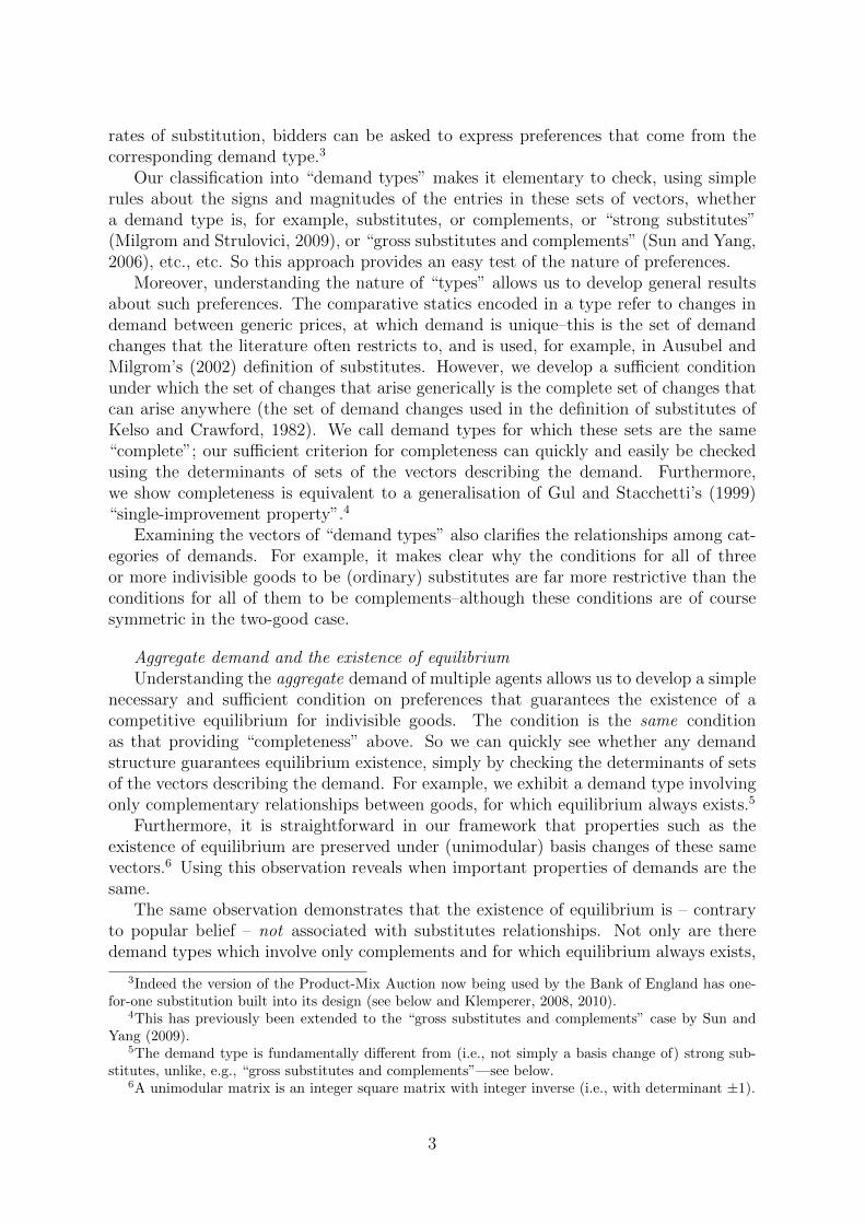
A simple example is shown in Figure 1. The agent’s valuations are u(0, 0) = 0,u(1, 0) = 5 and u(0, 1) = 4. So its demand is for precisely one of these bundles in eachof the three regions labelled, but switches from one bundle to another along the linesdrawn.

The following subsections describe properties of THs, and also how the structure ofthe agents’ demands can be recovered from them. The ‘tropical’ concepts may at firstsound alien, but many aspects of working in price space should in fact be very naturalto economists.

15We can, of course, model different units of a homogeneous good which are priced independently,by simply treating them as different goods.

16We follow the mathematical literature in this slight abuse of notation.17See Mikhalkin (2004) and others. In fact, Mikhalkin (2004) takes the tropical hypersurface asso-

ciated to u to be the non-smooth locus of p 7→ maxx∈A{x.p− u(x)}. Thus our tropical hypersurfacesare ‘upside down’ compared with his. Mikhalkin’s convention is not universal; Maclagan and Sturmfels(2009) take the non-smooth locus of p 7→ minx∈A{u(x)+x.p}, which defines tropical hypersurfaces the‘same way up’ as ours, albeit shifted. Our convention seems the natural one from an economic point ofview: we maximise surplus, that is, the value of a bundle minus its cost.

7

p

R=(5,4)

(0,0) demanded

(0,1) demanded

(1,0) demanded

L

1

p2

B

LA

LC

Figure 1: A simple tropical hypersurface (TH). The bundle demanded on each side ofthe TH is labelled.

2.2 The Tropical Hypersurface: associating geometric objectswith demand

We start by considering the local structure of a TH. Given a price p and its demandset Du(p), we ask for what other prices p′ the demand set is the same, or closely related.

Definition 2.1.

1. The cell interior of the TH Tu at a price p consists of points p′ such that Du(p) =Du(p

′).18 A subset of Tu is a cell interior if it is the cell interior at some point inTu.

2. A subset of Tu is a cell if it the closure of a cell interior of Tu.

3. The affine span of a cell of Tu is the smallest affine space containing the cell.19

4. The boundary of a cell of Tu consists of those points in the cell that are not in itscell interior.

Note that the cell interior is the largest set that is both contained in the cell and openin the affine span of the cell.20

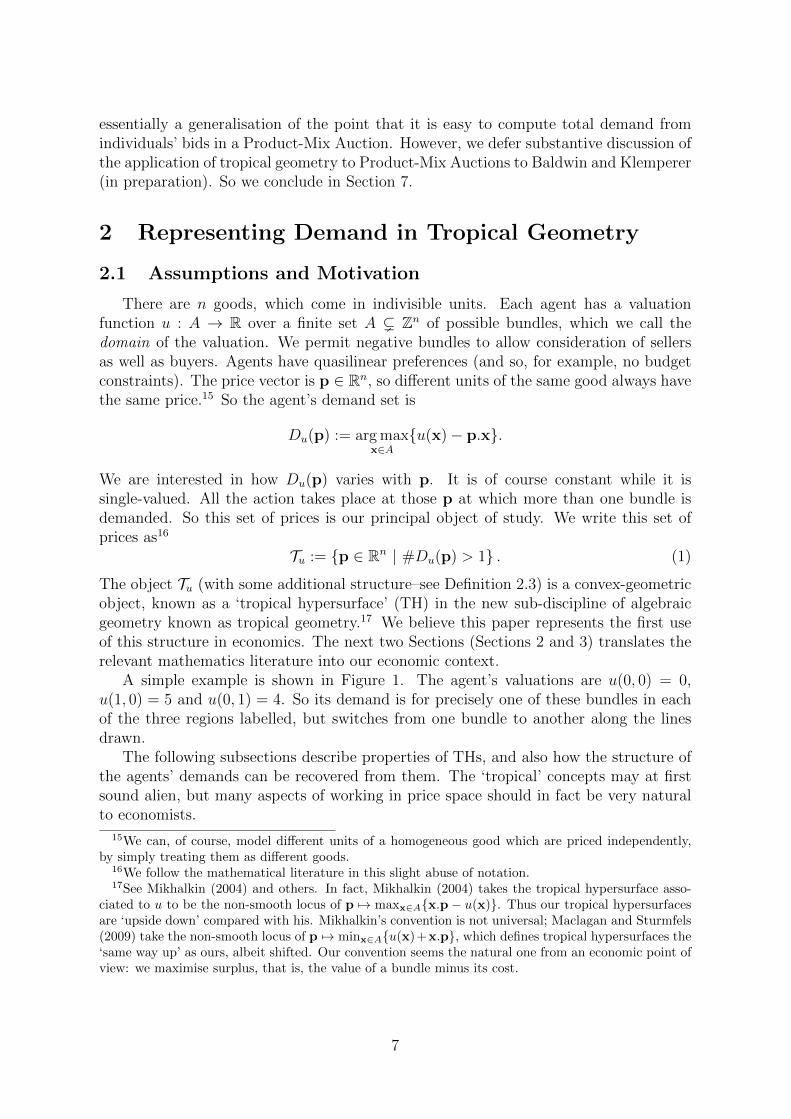
We call a cell of dimension k a k-cell,21 and call an (n− 1)-cell a facet.Figure 1 illustrates these concepts. The three line-segments LA, LB and LC in the

figure do not include the point R. Each of these line-segments is a cell interior: Du(p) =

18Note that cells are subsets of the TH Tu, and not, as one might intuitively guess from looking atFigure 1, the open areas around the sides of the TH; these are the ‘unique demand regions’.

19Recall that an affine space in Rn is a parallel shift of a linear subspace, that is, a set {v+c | v ∈ U}for some linear subspace U ≤ Rn and some fixed vector c.

20See the equations for the three objects, given below. One might strictly refer to the ‘cell interior’as the relative interior of the cell.

21To be precise, the dimension of a cell is the dimension of its affine span.

8

R

p2

p1

Figure 2: Cell interiors do not intersect; the line segments on either side of R are distinctcells.

{(0, 0), (1, 0)} in LA, Du(p) = {(0, 0), (0, 1)} in LB, and Du(p) = {(1, 0), (0, 1)} in LC .The point R is also a cell interior: Du(R) = {(0, 0), (1, 0), (0, 1)}. The correspondingcells are the unions of these cell interiors with their limit points: LA ∪ R is thus a cell,and indeed a facet; so are LB ∪R and LC ∪R. Finally, R itself is a 0-cell.

The price R is also the boundary of each of the 1-cells LA∪{R}, LB∪{R}, LC∪{R}.(The 0-cell R has no boundary.) Note that the price R is contained in four cells, buteach price in the TH is contained in precisely one cell interior. Finally, the affine span ofany cell is the set of all prices at which the agent is indifferent between all the bundles inthe cell, so the affine spans of LA∪R, LB∪R, and LC∪R, are the entire lines containingthose line-segments, while the affine span of R is the point R itself.

It is immediate that:

I There are finitely many distinct cells, and the TH is the union of these.

II The cell interiors do not intersect.

Figure 2 illustrates the latter point: although the TH is ‘two line segments crossingat a point’, it has four 1-cells with distinct interiors (and also a single 0-cell at R).

Furthermore Definition 2.1 implies that for a price p′ to be in the cell interior corre-sponding to a set of bundles Du(p), the agent must be indifferent between those bundles,that is, p′.(x − x′) = u(x) − u(x′) for all x,x′ ∈ Du(p), and the agent must strictlyprefer these bundles to all others, that is, p′.(x− x′′) < u(x)− u(x′′) for all x ∈ Du(p)and x′′ ∈ A\Du(p). The cell corresponding to this cell interior contains its limit points,so a price p′ is in the cell if the bundles in Du(p) are weakly preferred to all others atthis price; that is, we weaken the strict inequality above to a weak inequality (whilemaintaining the indifference between bundles in Du(p)).22 So a cell is the intersectionof a finite number of half-spaces (sets {p′ ∈ Rn | p′.v ≤ α} for some v ∈ Rn and someα ∈ R). Thus:

22It follows that we could alternatively define a cell as those points p′ such that Du(p) ⊆ Du(p′) forsome demand set Du(p).

9

III Each cell is a closed convex polyhedral set in Rn.

The affine span of the cell corresponding to Du(p) is simply those p′ such thatp′.(x− x′) = u(x)− u(x′) for all x,x′ ∈ Du(p). So the affine span of the cell is parallelto a linear subspace of Rn, and, since x,x′ ∈ Zn, we have:

IV The slope of the affine span of each cell is rational.

Finally, the boundary of the cell corresponding to Du(p) is those p′ such that at leastone of the weak inequalities p′.(x − x′′) ≤ u(x) − u(x′′) for x ∈ Du(p), x′′ ∈ A\Du(p)holds with equality. Such points therefore also lie in a lower dimensional cell, so byrestricting a suitable choice of inequalities to be equalities, we have:

V The boundary of a k-cell is a union of a finite number of (k − 1)-cells.

On the other hand, any (k − 1)-cell lies in the boundary of some k-cell (since, fromthe equations defining any (k− 1)-cell, we can obtain the equations defining some k-cellby weakening one or more of the equalities). It follows that a TH is contained in theunion of its facets.

We can therefore conclude that every TH for demand over n distinct goods can beunderstood as an (n− 1)-dimensional rational polyhedral complex :

Definition 2.2 (Mikhalkin, 2004, Definitions 1 and 2). A subset Π ( Rn is a rationalpolyhedral complex if it is a finite union of closed sets in Rn called cells which satisfyproperties I-V above. Π is k-dimensional if it is contained in the union of its k-cells.

By definition, demand in the complement of a TH is unique. We call a connectedcomponent of the complement of a TH a unique demand region (UDR). Demand isconstant in each UDR, since the bundle demanded cannot change without the pricecrossing the TH. But to understand how demand changes as we move between UDRs,we need one additional type of information: ‘weightings’ on the facets.

Let F be a facet and let bundles x and x′ be demanded in the UDRs on either side.So at prices p ∈ F , the agent is indifferent between x and x′, that is, u(x) − p.x =u(x′) − p.x′. The crucial point is that because p.(x′ − x) is therefore a constant forthese prices, the vector x′ − x is normal to F . Call the greatest common divisor of theentries of x′ − x the weight of the facet, w(F ). So vF := 1

w(F )(x′ − x) is a primitive

integer vector (that is, the greatest common divisor of its entries is 1), and it pointsfrom the UDR where x′ is demanded to the UDR where x is. But since F is (n − 1)dimensional, its normal direction is unique, so there is a unique primitive integer normalvector pointing from the UDR of x′ to that of x. Thus knowing only F , w(F ) and xallows us to derive vF , and hence x′. It therefore follows that if we know demand in anyone UDR, we can find demand everywhere from knowing the set of facets (and hencetheir primitive integer normal vectors) and their weights.

A rational polyhedral complex is described as weighted if a positive integer weightis attached to each facet. We provide examples in 2.4.

Understanding these weightings allows us to now give the full, formal definition of atropical hypersurface – recall that we have so far worked only with the underlying set.For completeness we repeat the definition of that set here, and so:23

23These definitions are mathematically identical to those of Mikhalkin (2004 and subsequent work),but the mathematical literature has not, of course, interpreted them in an economic context (that is,understood the Du(p) as demand sets).

10

Definition 2.3 (Mikhalkin, 2004, Example 2). Let A ( Zn be a finite set and letu : A→ R be any function. Then the tropical hypersurface Tu associated with u is theweighted rational polyhedral complex such that:

1. its underlying set is {p ∈ R | #Du(p) > 1};

2. the weight w(F ) of the facet F is the integer defined by w(F )vF = x′−x, in whichx′ is demanded in the UDR on one side of F , and x is demanded in the UDR onthe other side, while vF is the primitive integer normal vector pointing from theformer to the latter.

We will see that the TH captures all the information we might ever need to knowabout an agent’s demand and valuation function, if the latter is concave in the standardsense:

Definition 2.4. A function u : A→ R is concave if (ConvA) ∩ Zn = A and if u can beextended to a weakly concave function on Rn.

It is a standard result that concave functions are precisely those for which there are nobundles in A that are never demanded (see, e.g., Milgrom and Strulovici, 2009, Theorem1). That is:

Lemma 2.5. Let A ⊂ Zn. A function u : A → R is concave iff, for all x ∈ A, thereexists p ∈ Rn such that x ∈ Du(p).

Note, however, that we do not assume that all valuations are concave.It will be very important in our considerations of equilibrium (see Section 6) to know

that, if bundles are demanded, they are demanded at the ‘natural’ price:

Lemma 2.6 (Pseudo-equilibrium Prices Lemma, Milgrom and Strulovici, 2009, Propo-sition 2). Let u be any valuation function. Suppose p is any price vector, and x is aninteger bundle in ConvDu(p). If there exists any price vector p′ such that x ∈ Du(p

′),then x ∈ Du(p).

Proof. For all xβ ∈ Du(p), we know u(x) − p.x ≤ u(xβ) − p.xβ, with equality onlyif x ∈ Du(p). So if x ∈ ConvDu(p), i.e., x =

∑β λβx

β for some λβ ∈ [0, 1] with∑β λβ = 1, then it follows that u(x) − p.x =

∑β λβ (u(x)− p.x) ≤

∑β λβu(xβ) −∑

β λβp.xβ =

∑β λβu(xβ) − p.x and so, simplifying, that u(x) ≤

∑β λβu(xβ), with

equality only if x ∈ Du(p).Now suppose x ∈ Du(p

′). Then u(x)−p′.x ≥ u(xβ)−p′.xβ for all xβ so we similarlyshow that u(x) ≥

∑β λβu(xβ). Hence, if x ∈ Du(p

′) for any p′, then x ∈ Du(p). �

2.3 Associating demand with geometric objects

When does a weighted rational polyhedral complex depict a valid demand of someagent?

If we construct a TH by starting from some valuation function u, then the weightswe attach will necessarily be coherent, in the sense that if we cross facets by passingthrough a sequence of UDRs that ends where it started, we must demand at the endprecisely what we demanded at the beginning. In particular, the TH will satisfy thebalancing condition:

11

Definition 2.7 (Mikhalkin, 2004, Definition 3). An (n − 1)-dimensional weighted ra-tional polyhedral complex Π ( Rn is balanced if for every for every (n− 2)-cell G ( Π,the weights w(Fj) on the facets F1, . . . , Fl that are adjacent to G, and primitive integernormal vectors vFj

for these facets that are defined by a rotational direction about G,

satisfy∑l

j=1w(Fj)vFj= 0.24

Note that there do not necessarily exist weights to balance a general rational poly-hedral complex.25 However, the balancing condition is in fact the only condition thata weighted rational polyhedral complex has to satisfy to be the TH of some valuationfunction:

Theorem 2.8 (Mikhalkin, 2004, Proposition 2.4; also Mikhalkin, 2005, Theorem 3.15).Suppose that Π ( Rn is an (n − 1)-dimensional balanced weighted rational polyhedralcomplex.26 Then there exists a finite set A ( Zn and a function u : A→ R such that Πis the TH, Tu.

The correspondence between a TH and its associated set A and function u is notunique, but the ambiguities are trivial if u is concave. Clearly, adding a constant to u(x)leaves the TH unchanged, as does increasing every available bundle by a fixed bundleand making a corresponding shift in the valuation (though the bundle demanded in eachUDR will then also be increased by the fixed bundle). That is, if A′ = {x + c | x ∈ A}and u′(x + c) = u(x) + α for all x ∈ A, some c ∈ Zn, and some α ∈ R, then Tu′ = Tu.(See Example 2.12 for an example of such a shift).

Furthermore, any non-concave u has the same TH as the minimal weakly-concavefunction that weakly exceeds it everywhere on A. To see this, observe that if a bundleis never demanded then its precise value to the agent is immaterial, so we can increaseits value up to the threshold at which it is just marginally demanded for some price(s)without altering the shape or properties of the TH. Doing this for all never-demandedbundles removes any non-concavities in the valuation function. It is also now clear thatif two agents have valuations u and u′, respectively on different sets of bundles A andA′, but their convex hulls in Rn, which we write ConvA and ConvA′, coincide; and ifu is the minimal concave function on ConvA such that u ≥ u on A, and is also theminimal concave function on ConvA such that u ≥ u′ on A′; then Tu = Tu = Tu′ .27

Summing up:

Theorem 2.9 (Mikhalkin, 2004, Remark 2.3). There is a 1-1 correspondence betweenTHs with an identified ‘demand 0’ UDR, and pairs (u,A), where A ( Zn is finite and

24To choose a rotational direction around G, pick a 2-dimensional affine subspace H of Rn orthogonalto G, such that the intersection of each Fj with H is 1-dimensional. The intersection of H with theTH is then a collection of 1-cells meeting at the 0-cell which is G∩H. An ordinary choice of rotationaldirection in this two-dimensional picture gives a rotational direction around G in Rn.

25For example, in two dimensions, consider three 0-cells, each with three adjacent facets. If eachpair of 0-cells has an adjacent facet in common, the six weights must satisfy six balancing conditions(that is, three equations in each of the two dimensions). But since the balancing conditions are triviallysatisfied by setting all weights equal to zero, the conditions can only be satisfied by positive integerweights if the conditions are not linearly independent–which is non-generic.

26Strictly speaking, of course, Π is a subset of the space Rn and has weights. As before, we followMikhalkin and the

mathematical literature in our presentation.27We defined u on ConvA ( Rn, but it still defines a TH if it is restricted to (ConvA) ∩ Zn.

12

convex in Zn, u is a weakly-concave, function u on A, for which u(0) = 0 and 0 isdemanded where specified.

Thus we have full equivalence between THs and weakly-concave valuation functions(such that u(0) = 0 and 0 is demanded in a specified UDR). Note, in particular, thata given set in Rn is the TH of some quasilinear demand if and only if it is a rationalpolyhedral complex and there exist weights for the facets such that it is balanced.Although we do not restrict attention to concave valuation functions–indeed Section 6.3will ask when an aggregate valuation is concave–understanding of the concave case isimportant.

Similarly, we do not restrict attention to what is demanded in UDRs, but doing so isan important first step. Generically all prices are in a UDR so, as noted above Definition2.3, given any TH and a specified ‘zero demand’ UDR we can easily work out what isdemanded for a generic price. And it is particularly straightforward to relate propertiesof demand such as substitutes or complements to the geometry of the TH; see Section4.

2.4 Demand examples

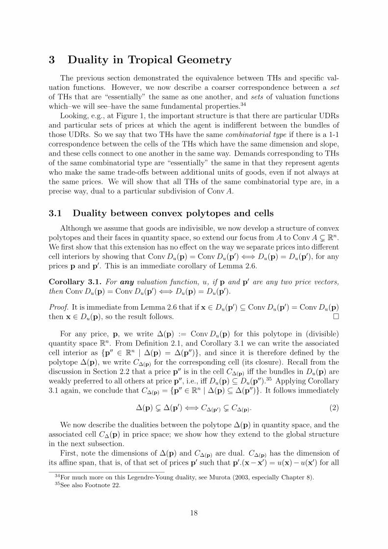
Example 2.10. Let A = {x ∈ Z2≥0 | x1 + x2 ≤ 2} and let u : A → R be as follows

(we arrange the terms in this “back-to-front” way to correspond to the fact that smallerquantities will appear higher in, and further right in, the TH; this convention will beparticularly helpful later):

x1 = 2 x1 = 1 x1 = 0 u7 6 0 x2 = 0

9 4 x2 = 18 x2 = 2

.

The TH associated with the agent’s valuation, u, is shown in Figure 3, in which wehave additionally marked in red the bundle demanded by this agent in each UDR. Thefacet between the UDRs in which (0, 0) and (0, 2) are demanded has weight 2. For pin this facet (that is, for p2 = 4 and p1 > 6) we have Du(p) = {(0, 0), (0, 1), (0, 2)}; inparticular the bundle (0, 1) is demanded for some price and the function is concave. Anotherwise-identical valuation u′ in which u′(0, 1) < 4 would give rise to the same TH,but would not be concave; (0, 1) would not be demanded for any price.

It is easy to work out, from the TH, which bundle is demanded in each UDR, if onealready knows what is demanded in any one UDR. If x1 = x2 = 0 in the top right UDRwe can simply “walk around” the diagram, adding to x1 (x2) the weight of any facetcrossed times the first (second) coordinate of the primitive integer facet normal. Thusstarting from the top right UDR, crossing the vertical facet with normal (1, 0), that is,{p ∈ R2 | p1 = 6, p2 > 4}, changes demand from (0, 0) to (1, 0); from there, crossing thefacet with normal (−1, 2) changes demand to (0, 2), as may also be seen by crossing theweight-2 horizontal from (0, 0) downwards; and so on.

Example 2.11. It will be useful later to discuss very simple examples of substitutesand complements demands: if A = {0, 1}2, then u1 : A→ R and u2 : A→ R defined as

13

p1

p2

1

2

3

4

5

1 2 3 4 5 6 7

2

00

(0,0)

(0,2)

(1,0)(2,0)

(1,1)

Figure 3: The TH of Example 2.10, with the bundle demanded in each UDR marked inred.

follows are demands for substitutes and complements, respectively, and their THs areshown in Figures 4a and 4b.28

x1 = 1 x1 = 0 u1

1 0 x2 = 01 1 x2 = 1

andx1 = 1 x1 = 0 u2

0 0 x2 = 01 0 x2 = 1

.

p1

p2

1

1

(a) Tu1 .

p1

p2

1

1

(b) Tu2 .

Figure 4: The THs of Example 2.11.

Clearly each TH has four UDRs in which these agents demand the bundles (0, 0),(0, 1), (1, 1), and (1, 0), respectively, as one moves clockwise around the UDRs startingat the top right–as is also easily confirmed by adding the appropriate primitive integerfacet normal on every crossing between UDRs.

Example 2.12. To illustrate the case in which an agent both buys and sells goods, letA = {(0, 0), (−1, 1)} and let u(0, 0) = 0, and u(−1, 1) = −3. This corresponds to an

28The TH of Figure 4a appears to be a translation of Figure 1, but there is an important distinction.In Figure 1 the domain is {(0, 0), (0, 1), (1, 0)}, so the TH has only one 0-cell; here, u1 has domain{0, 1}2, and its TH has two 0-cells. (If we restricted u1 to the domain {(0, 0), (0, 1), (1, 0)} its TH wouldcoincide with Tu1 on R2

≥0 but have only one 0-cell.)

14

p1

p2

1 2 3

Figure 5: The TH of Example 2.12.

(1,1,1)

p1

p2

p3

Figure 6: The TH of Example 2.13.

agent who can convert one unit of good 2 into one unit of good 1 at a cost of 3; theagent will therefore buy one unit of good 2 and sell one unit of good 1 if p1 − p2 > 3,and do nothing if p1 − p2 < 3. See Figure 5.

Observe that it would be economically identical if the agent were initially endowedwith one unit of good 1 which it would be prepared to trade for a unit of good 2 if theprice difference were at least 3–the agent’s choices of what to buy and sell would dependon the prices in exactly the same way. This corresponds to simply shifting the valuationto the right so A = {(1, 0), (0, 1)} with u(1, 0) = 0 and u(0, 1) = −3. Note that in thiscase (0, 0) /∈ A. We need not (and do not) prescribe that the zero bundle has to be anavailable option.

Example 2.13. For a simple 3-dimensional example, let A = {x ∈ Z3≥0 | x1 +x2 +x3 ≤

1} and let u(0, 0, 0) = 0 and u(1, 0, 0) = u(0, 1, 0) = u(0, 0, 1) = 1. The TH is given inFigure 6. Now, the facets are 2-dimensional (pieces of planes), there are additionally1-cells (lines along which these facets meet), and a 0-cell (point at which these linesmeet). Three of these facets, having normals (1, 0, 0) (dark-green facet), (0, 1, 0) (redfacet), and (0, 0, 1) (turquoise facet), border the UDR in which (0, 0, 0) is demanded;this UDR is of course {p ∈ R3 | p1, p2, p3 > 1}. Crossing any one of these facets takesus to the UDR in which the corresponding bundle is demanded. We swap betweenthe latter UDRs by crossing the remaining three facets, which have normals (1,−1, 0)(orange facet), (0, 1,−1) (bluish-purple facet) and (1, 0,−1) (yellow facet).

15

2.5 Classic models interpreted in our framework

Many classic models in which agents have quasi-linear demands for indivisible goodsare special cases of our framework:

First, it is trivial that Bikhchandani and Mamer (1997) is the restriction of our modelto A = {0, 1}n.

Example 2.14 (Workers and Firms–Kelso and Crawford, 1982, and Hatfield and Mil-grom, 2005). Kelso and Crawford (1982) model matching between workers, desiring atmost one job, and firms, interested in hiring many workers, who they regard as substi-tutes. Thus each ‘good’ is a contract between a worker and a firm, and its ‘price’ is thesalary.

To represent this in our framework, let i ∈ {1, . . . ,m1} be the workers, and j ∈{1, . . . ,m2} be the firms, so there are n = m1m2 contracts which we can index as(i, j). Then worker i has valuation ui : Ai → R with domain Ai := {0,−e(i,j) | j =1, . . . ,m2} ( {−1, 0}n. That is, we regard it as a seller of its labour, and it has no pref-erences over the sale of other workers’ labour. On the other hand, firm j has valuationuj : Aj → R with domain Aj := {x ∈ {0, 1}n | x(i,j′) = 0 for j′ 6= j} ( {0, 1}n. That is,it is only able to buy workers, and only has preferences over the workers it ‘buys’ itself.Note that the total set of meaningful bundles {−1, 0, 1}n is the (Minkowski) sum of allthe sets Ai and Aj; in Section 6 we will refer to this set as the domain of the aggregatevaluation. We discuss Kelso and Crawford’s ‘gross substitutes’ condition in Section 5.3.

Hatfield and Milgrom (2005) consider matchings between firms and workers withmore general ‘contracts’ than just salaries, but their model can be embedded in Kelsoand Crawford (1982),29 so can also be presented in our framework.

Example 2.15 (General ‘Trading Networks’–Hatfield et al., 2013, Ostrovsky, 2008).Models such as Hatfield et al. (2013) consider agents each of whom can both buy andsell. Each ‘good’ in these models is the trade of a single unit of a product betweena specified buyer and a specified seller; additional units of the identical product aretreated as separate trades and may have differing prices.30

To embed this in our framework, let n be the total number of feasible trades, andfor j = 1, . . . , n let b(j) be the buyer and s(j) be the seller in the (potential) trade.Then agent i has valuation ui : Ai → R with domain Ai ⊆ {x ∈ {−1, 0, 1}n | xj < 0⇒s(j) = i; xj > 0 ⇒ b(j) = i}. That is, agent i considers bundles in which the goods itsells are in non-positive quantities, and the goods it buys are in non-negative quantities.However, agent i need not consider the whole of this set; there may be bundles that areinfeasible (for example, if it cannot sell good 1 unless it also buys one of goods 2, 3 or 4,then bundle −e1 is not in the domain Ai). Example 2.12 is a special case of this model.

We discuss Hatfield et al. (2013)’s ‘full substitutability’ condition in Section 5.3.

Example 2.16 (Coalition Formation with Transferable Utility). 31 A classic literature

29Echenique (2012) shows this. Hatfield and Kojima (2010) does not fit into our framework, since itis inconsistent with quasi-linear preferences (see the discussion in Echenique, 2012).

30Hatfield et al. (2013) impose no restrictions on the shape of the ‘trading network’ formed by thefeasible trades, so thus generalise the ‘two-sided matching literature’ started by Gale and Shapley (1962)in the case in which all preferences are quasilinear. (Ostrovsky, 2008 is also related, but does not requirequasi-linearity and has discrete prices.)

31Cf. Koopmans and Beckmann (1957), Shapley and Shubik (1971), Kaneko and Wooders (1982),Eriksson and Karlander (2001), Talman and Yang (2011) and Chiappori et al. (2012).

16

models coalition formation – typically in a bipartite context. Each person (we do notrefer to people as ‘agents’, since they will not take the roles of ‘agents’ in our framework)gets intrinsic value from being a member of a coalition. However, the surplus of anycoalition can be transferred among people within that coalition, in the form of side-payments. Each person has quasi-linear utility in the intrinsic value of the coalitionand this side-payment. We typically seek a ‘stable’ outcome, in which every person isassigned to precisely one coalition (perhaps entailing them being alone) and no subsetof people can all (strictly) gain by deviating from their prescribed coalition and forminga new one.32

We model this in our framework as follows: the ‘agents’ are potential coalitions, whobuy ‘goods’, which are people. The ‘price’ paid by an ‘agent’ for a good is the surplus(including any side payments) the person receives in that coalition.

So the goods available are ‘person-goods’ indexed i = 1, . . . , n. The bundles x ∈{0, 1}n denote sets of ‘person-goods’, where xi = 1 iff i is included in the set. We let Bbe the set of feasible coalitions; in general, not every set of people is a feasible coalition,but we include a distinct ‘coalition-agent’ for every coalition that is feasible, includingany feasible coalition that yields zero utility (for example, a given person being alonemay be a feasible coalition that yields zero utility).

We consider the people as each being assigned to a coalition and immediately handingtheir value in that coalition to the coalition-agent itself. Some of this money is thentransferred back to the people in the coalition: pi is the price the coalition-agent paysfor person-good i. If a person-good is priced at pi then the net side-payment to thisperson from coalition-agent x is thus pi− ui(x), where ui : {x ∈ B | xi = 1} → R is theindividual’s intrinsic valuation function on coalitions. Hence, the net utility to person iat this stage is simply ui(x)+pi−ui(x) = pi. (There will in general be additional surplusto distribute among the coalition members at a later stage; we think of the ‘price’ asthe minimum that needs to be offered to buy the person-good.)

Thus we think of each person as stating a price for himself33 and seeing whichcoalition will buy; although his intrinsic values for the different coalitions may differ, hisnet utilities when he receives this price are all the same.

The ‘coalition-agent’ corresponding to coalition x obtains the sum of the individualvalues of the people in that coalition minus the ‘prices’ it pays for those people, if theyare all assigned to it. So the domain of the coalition-agent’s valuation is Ax := {0,x}and we define ux(0) = 0 and ux(x) =

∑i : xi=1 u

i(x). If the vector of prices for person-goods is p, the coalition-agent’s net utility from bundle y is ux(y)− p.y. So if the sumof the ‘prices’ of all the people is at most the total surplus from the coalition, that is, thecoalition-agent can make side-payments that give each person the utility he demands,then the coalition-agent’s maximising bundle is x; otherwise it is 0. Thus the formationof coalitions is just the maximising behaviour of coalition-agents.

We discuss the formation of stable coalitions in equilibrium in Section 6.2.

32We will see (in Section 6.2) that in this setting the stable outcomes will coincide with the coreallocations (and also coincide with the core allocations of a game with fully transferable utility, i.e.,across as well as within coalitions).

33We prefer the use of the female pronoun for people, except where–as here–they are treated as goodsto be priced and traded.

17

3 Duality in Tropical Geometry

The previous section demonstrated the equivalence between THs and specific val-uation functions. However, we now describe a coarser correspondence between a setof THs that are “essentially” the same as one another, and sets of valuation functionswhich–we will see–have the same fundamental properties.34

Looking, e.g., at Figure 1, the important structure is that there are particular UDRsand particular sets of prices at which the agent is indifferent between the bundles ofthose UDRs. So we say that two THs have the same combinatorial type if there is a 1-1correspondence between the cells of the THs which have the same dimension and slope,and these cells connect to one another in the same way. Demands corresponding to THsof the same combinatorial type are “essentially” the same in that they represent agentswho make the same trade-offs between additional units of goods, even if not always atthe same prices. We will show that all THs of the same combinatorial type are, in aprecise way, dual to a particular subdivision of ConvA.

3.1 Duality between convex polytopes and cells

Although we assume that goods are indivisible, we now develop a structure of convexpolytopes and their faces in quantity space, so extend our focus from A to ConvA ( Rn.We first show that this extension has no effect on the way we separate prices into differentcell interiors by showing that ConvDu(p) = ConvDu(p

′)⇐⇒ Du(p) = Du(p′), for any

prices p and p′. This is an immediate corollary of Lemma 2.6.

Corollary 3.1. For any valuation function, u, if p and p′ are any two price vectors,then ConvDu(p) = ConvDu(p

′)⇐⇒ Du(p) = Du(p′).

Proof. It is immediate from Lemma 2.6 that if x ∈ Du(p′) ⊆ ConvDu(p

′) = ConvDu(p)then x ∈ Du(p), so the result follows. �

For any price, p, we write ∆(p) := ConvDu(p) for this polytope in (divisible)quantity space Rn. From Definition 2.1, and Corollary 3.1 we can write the associatedcell interior as {p′′ ∈ Rn | ∆(p) = ∆(p′′)}, and since it is therefore defined by thepolytope ∆(p), we write C∆(p) for the corresponding cell (its closure). Recall from thediscussion in Section 2.2 that a price p′′ is in the cell C∆(p) iff the bundles in Du(p) areweakly preferred to all others at price p′′, i.e., iff Du(p) ⊆ Du(p

′′).35 Applying Corollary3.1 again, we conclude that C∆(p) = {p′′ ∈ Rn | ∆(p) ⊆ ∆(p′′)}. It follows immediately

∆(p) ( ∆(p′)⇐⇒ C∆(p′) ( C∆(p). (2)

We now describe the dualities between the polytope ∆(p) in quantity space, and theassociated cell C∆(p) in price space; we show how they extend to the global structurein the next subsection.

First, note the dimensions of ∆(p) and C∆(p) are dual. C∆(p) has the dimension ofits affine span, that is, of that set of prices p′ such that p′.(x−x′) = u(x)−u(x′) for all

34For much more on this Legendre-Young duality, see Murota (2003, especially Chapter 8).35See also Footnote 22.

18

x,x′ ∈ Du(p). If ∆(p) is k-dimensional, these equations impose k linearly independentconstraints on such p′, so dimC∆(p) = n− k.

Next observe the affine spans of these sets are orthogonal: since p′.(x−x′) is constantfor all p′ ∈ C∆(p) and all x,x′ ∈ Du(p), we have (p′ − p′′).(x − x′) = 0 for anyp′,p′′ ∈ C∆(p) and x,x′ ∈ ∆(p). So all prices in C∆(p) lie in a subspace of Rn orthogonalto any x − x′ where x,x′ ∈ ∆(p), and all bundles in ∆(p) lie in a subspace of Rn

orthogonal to p′ − p′′ for any p′,p′′ ∈ C∆(p).Therefore, any (n−1 dimensional) facet F = C∆(p) (in price space) corresponds to a

1-dimensional polytope, i.e., a line-segment, ∆(p), orthogonal to it (in quantity space).And if x and x′ are the endpoints of the line-segment ∆(p), then x−x′ = wvF for somew ∈ Z, where vF is a primitive integer vector in the direction of ∆(p), i.e. in the normaldirection to F ; let us chose vF so that w > 0. And since the bundles demanded in theUDRs on either side of F are precisely the vertices at the endpoints of ∆(p), it alsofollows that this w is the weight of F , as defined in Section 2.2. In words, the “length”of the line-segment ∆(p) in quantity space is the weight of its corresponding facet inprice space.

3.2 The subdivided Newton Polytope

Convex geometry now provides a clever trick to find the set of all the polytopes,∆(p), very quickly, and see how they fit together in quantity space. From this it is easyto see how the cells of the TH fit together in price space.

The condition that a bundle x′ ∈ Du(p) maximises the agent’s surplus at price pcan be re-written using vectors in Rn+1 as (−p, 1).(x, u(x)) ≤ (−p, 1).(x′, u(x′)) forall x ∈ A. So the points (x, u(x)), for all x ∈ A, must lie in a particular half-spaceof Rn+1. Furthermore all the other bundles x′′ which are optimal at the same price psatisfy (−p, 1).(x′′, u(x′′)) = (−p, 1).(x′, u(x′)) and so all lie on the hyperplane in Rn+1

bounding this half-space. Hence every set ∆(p) ( i.e. any ConvDu(p)) is the projectionto the first n coordinates of a face of the set

A := Conv{(x, u(x)) ∈ Rn+1 | x ∈ A}. (3)

Conversely, consider any face ∆ of A on the ‘upper side’ with respect to the finalcoordinate (i.e., any face such that points with a slightly lower final coordinate than

those in the face are in A, and those with a slightly higher final coordinate are not). ∆

is the intersection of A with some hyperplane {y ∈ Rn+1 | v.y = α} for some α ∈ R,and some normal vector v ∈ Rn+1. We know A is contained in the half-space below thehyperplane with respect to the final coordinate. Renormalising so the final coordinateof v is 1, so v = (−p, 1) for some vector p ∈ Rn, the face ∆ is the convex hull of allpoints (x′, u(x′)), where x′ is in A, satisfying (−p, 1).(x, u(x)) ≤ (−p, 1).(x′, u(x′)) for

all x ∈ A; that is, u(x′)− p.x′ is maximal over bundles in A. Thus the projection of ∆to its first n coordinates is exactly ∆(p) for this p.

Summarising, each upper face of A is the set (x, u(x)) that are maximal when viewedin the direction of some vector (−p, 1); the face then projects to ∆(p). And conversely,

any set ∆(p) is the projection of an upper face of A. So the information about thedemand sets is contained in the projections of these faces, that is, in the collection of

19

sets{x | (x, u(x)) ∈ ∆

}, where ∆ is an upper face of A.

Definition 3.2.

1. The subdivision of ConvA given by the projections of the upper faces of A ontoConvA is a subdivided Newton polytope (SNP).36

2. The image ∆ of a k-dimensional face ∆ of A is a k-face of the SNP.

We give an example of how to construct an SNP in practice in Section 3.3.Since, for k < n, any k-face of A is the face of an n-face of A, it is sufficient to

consider only the maximal faces of A to identify the full SNP structure.In particular, an SNP n-face, ∆, is the projection of an upper n-face ∆ of A. But

since ∆ is n-dimensional, there is a unique hyperplane of Rn+1 passing through it, andso a unique normal vector of the form (−p, 1). So the projection ∆ of ∆ to ConvA isexactly ∆(p) = ConvDU(p), and is not ∆(p′) for any p′ 6= p. So p is the only priceat which all these bundles are demanded, and {p} is therefore a 0-cell in the TH, i.e.{p} = C∆(p).

At the other extreme, for any 0-face {x} of the SNP, there exist prices p at which

(x, u(x)) is the unique point of A intersecting a supporting hyperplane normal to (−p, 1).For any such p we know {x} = Du(p). Furthermore, if any such p is changed infinites-imally in any coordinate direction, the point {(x, u(x))} is still the unique point of

A intersecting the corresponding supporting hyperplane. So the UDR in which x isdemanded, that is, the set of p such that {x} = Du(p), is (of course) n-dimensional.

Between these extremes, any upper k-face of A, where 2 ≤ k ≤ n − 1, is theintersection of A with any one of a range of hyperplanes in Rn+1. The vector (−p, 1)normal to any such hyperplane defines a price p lying in the corresponding (n − k)-dimensional cell interior of the TH.

Note also that, since ConvA need not in general be n-dimensional (see Example 2.12for an example in which it is not) the SNP need not have any n-faces; this correspondsto a TH with no 0-cells (such as that in Figure 5).

The fact that the SNP’s faces, ∆(p), are the projections of faces of a convex set tellsus how they fit together, and hence how the sets Du(p) fit together. If ∆(p) ( ∆(p′)for two faces of the SNP, then ∆(p) must be a face of the polytope ∆(p′). But recall(displayed equation 2) that ∆(p) ( ∆(p′) iff C∆(p′) ( C∆(p). As discussed above (at andbeneath point V of Section 2.2, ) the latter holds iff C∆(p′) is in the boundary of C∆(p).Moreover, ∆(p) and C∆(p) are orthogonal, as discussed in Section 3.1. So knowing howthe ∆(p) fit together in quantity space makes it immediately obvious how the C∆(p) fittogether in price space, and vice versa.

So the SNP tells us which cells must exist in the corresponding THs, their slopes,and how they are connected. In other words

Theorem 3.3 (Mikhalkin, 2004, Proposition 2.1.). For a given ConvA there is a 1-1correspondence between SNPs of THs and combinatorial types of THs.

36It is a subdivision of the set ConvA which is itself called a Newton polytope in (tropical) algebraicgeometry.

20

As noted above, this correspondence is coarser than the correspondence we describedin the previous subsection (Theorem 2.9): different valuations correspond to the sameSNP, and hence to a TH of same combinatorial type, even though the coordinates of theparts of the TH differ. However, this correspondence isolates the underlying propertiesof demands, specifically the sets of bundles one might ever be indifferent between, andthe trade-offs one might make.

Also, starting from any SNP, it is easy to find the combinatorial type of the TH,and so see which coordinates uniquely define the TH. The TH can then be completelyidentified using the valuation u. We illustrate this in Section 3.3.

Another important point follows: if A is small, it is easy to list all the possible SNPs,and hence also list all possible combinatorial types of THs for the set A. That is, wecan easily list every possible distinct structure of trade-offs that an agent might makebetween a given finite collection of goods.

Of course, we do not need to start with the SNP. Given the TH and an identified‘demand 0’ UDR, we can easily infer both A and the full SNP using the duality describedin this section.

Note, however, that if we do not know ex ante whether a TH is concave, then neitherthe TH nor the SNP can necessarily tell us which bundles are demanded in each cell ofthe TH. The information we do have is as follows:

Corollary 3.4. Let A be convex in Zn, let u : A→ R be a valuation, and consider thecorresponding SNP.

1. A bundle x ∈ A is a vertex of the SNP iff it is demanded in some UDR of thecorresponding TH.

2. If every bundle x ∈ A is a vertex of the SNP, then u is concave for every valuationu : A→ R such that Tu = Tu.

3. If a bundle x ∈ A is not a vertex of the SNP, there exist valuations u : A → Rsuch that Tu = Tu but x /∈ Du(p) for any p ∈ R.

Proof. 1 is clear from the previous discussion. 2 follows from Lemma 2.5. For 3, define uto be equal to u on the vertices of the SNP, and to be arbitrarily large negative numberson those bundles in A that are not vertices of the SNP. �

However, in quantity space we do not have an analogue of Theorem 2.8. Nor doesthere seem to be any simple analogue of Theorem 2.8’s easy balancing condition thatwould check whether a given subdivision is the SNP of a valuation function:

Fact 3.5. It is not the case that every subdivision of every Newton polytope is the SNPof some valuation function.

Proof. A counterexample is provided by Gathmann (2006, Figure 7). �

21

3.3 Examples

Example 3.6. Starting from a valuation function, a TH can easily be drawn by firstderiving the SNP, then using the SNP to draw the shape of the TH’s combinatorialtype, and finally using the valuations to fix the TH’s exact location in price space.

Figure 7 presents a valuation function u, both in the usual tabular representation,and by showing the permissible set of bundles A, as a subset of the lattice Zn, labelledwith their valuations. As before, the quantity of good 1 increases as we move to theleft, and the quantity of good 2 increases as we move down, in order to show the dualitybetween the SNP and the TH most clearly.

x1 = 2 x1 = 1 x1 = 0 u10 5 0 x2 = 012 8 7 x2 = 113 13 9 x2 = 2

(a) Tabular representation of the valua-tion.

0

7

9

5

8

13

10

12

13

x2

x =02

x =12

x =22x =

21 x =

11 x =

01

x1

(b) Each circled number gives the valueof the bundle in that position.

Figure 7: Alternative representations of a valuation function.

Figure 8 adds a third dimension to Figure 7b. Figure 8a shows the points (x, u(x))

0

7

9

5

813

1012

13

x1

x2

value

(a) The values (x, u(x)) for all x ∈ A.

x1

x2

value

(b) The upper surface of A.

Figure 8: Finding A in three dimensions.

22

x1

x2

Figure 9: The SNP.

for all x ∈ A, with the valuations u(x) drawn as lines connecting them to their associatedbundles, x, to make the relationships clearer. Figure 8b then pictures the upper surfaceof A, with those lines that correspond to bundles that are demanded for some price(s) inbold. Note that the valuation is non-concave and the bundle (1, 1) is never demanded.

The SNP is pictured in Figure 9. It is drawn without axes, since replacing A withA+ c for some c ∈ Zn and re-defining u to correspond gives us the same SNP and TH.A depiction of the SNP and an example of a TH of the corresponding combinatorialtype is given in Figure 10, colour-coded so that objects that are the geometric duals of

(a) The SNP, colour-coded.

2

p2

p1(b) A TH, colour-coded to correspond.

Figure 10: The SNP and a TH of the corresponding combinatorial type, colour-codedso that dual geometric objects have the same colours.

each other have the same colours as each other. That is, each point in the TH has thesame colour as its corresponding area in the SNP; each line-segment (facet) in the THhas the same colour as the line-segment (edge) in the SNP that it corresponds, and isorthogonal to; and the white areas (UDRs) in the TH correspond to the white points(bundles that are vertices) in the SNP.

Note that the black point in the SNP that represents the bundle (1, 1) has no object

23

2p2

p1(0,1)

(1,2)(3,3)

(4,2)

(5,7)

Figure 11: The TH of the valuation function presented in Figure 7.

corresponding to it in the TH–it is “hidden” inside the scarlet-coloured point in theTH. If that bundle’s valuation were greater so that, rather than the line correspondingto it in Figure 8b lying strictly below a plane coincident with A, the line instead justtouched that plane,37 then the bundle would be demanded at the price correspondingto the scarlet-coloured point in the TH. And if the bundle had a still higher valuation,that point in the TH would “open up” to form an area corresponding to the range ofprices at which the bundle would then be demanded.

The final SNP lattice point is coloured grey. It is not an SNP vertex, but lies within(horizontal) SNP edge of the same colour, which has “length” 2 (more precisely, thegreatest common divisor of the differences (2, and 0) between the co-ordinates of thebundles at the ends of this edge is 2). And this corresponds to the vertical grey facet inthe TH which is labelled “2”, reflecting its weight.

Finally, remember that Figure 10b shows only one of many THs of the combinatorialtype corresponding to the SNP in that figure; the SNP is silent on the lengths of thelines in its corresponding THs. However, the exact location of the TH for our specificset of valuations can easily be worked out from the valuations of different bundles: SeeFigure 11.

For example, it is clear from the valuations of bundles (1,0) and (0,1) that the topright (pinky-purple) point of the TH is at p = (5, 7), since 5 and 7 are the prices belowwhich the agent will first buy any of goods 1 and 2, respectively,when the other good’sprice is very high. And the coordinates of the purple point at the bottom right of theTH must be (4,2) since 9 − 7 = 2 is the incremental value of a second unit of good 2,when the agent has no unit of good 1, and 13 − 9 = 4 would be the further incrementin value from then also having a unit of good 1, etc.

We discussed above (Section 2.2; see especially Example 2.10) how the demand ineach UDR can easily be worked out from the TH.

37It is easy to compute that the valuation of this bundle would have to be 10 for this to happen.

24

Example 2.10 revisited. It is not hard to check that the SNP for Example 2.10 isas shown in Figure 12a. Two examples of THs of the corresponding combinatorial typeare given in Figures 12b and 12c.

(a)

2

(b)

2

(c)

Figure 12: (a) the SNP of Example 2.10; (b) and (c) two examples of THs of thecombinatorial type of Example 2.10.

Example 3.7. For a fixed A, it is easy to draw every possible SNP and so obtain everypossible combinatorial type of TH, thus enumerating all possible “essentially-different”structures of demand. We do this for A = {0, 1}2 in Figure 13.

It is not hard to see that Figure 13a applies when u(0, 0)+u(1, 1) < u(1, 0)+u(0, 1),so represents substitutes; Figure 13b applies when u(0, 0) + u(1, 1) = u(1, 0) + u(0, 1),so is additively separable demand; and Figure 13c applies when u(0, 0) + u(1, 1) >u(1, 0)+u(0, 1), so is complements. (Recall Figure 4.) Importantly, it is clear that theseare the only possibilities.

Observe that Figure 13b can be seen as a limit of Figure 13a (or, equivalently, Figure13c). In the TH, the two 0-cells become arbitrarily close and then coincide in the limit;

in the SNP, the faces of A tilt until they are coplanar when the SNP edge distinguishingthem disappears in this limit.

Likewise, any SNP in which the subdivision is not maximal (that is, additional valid(n− 1)-faces could be added) can be recovered by deleting (n− 1)-faces from some SNPwhose subdivision is maximal; the corresponding TH is a limit (or ‘degeneration’). Evenfor larger domains than A = {0, 1}2, we can efficiently enumerate all those combinatorialtypes of demand for which the SNP subdivision is maximal, knowing we can recover theremainder as their limits. We do this for A = {0, 1, 2} × {0, 1} in Figure 14.

(a) (b) (c)

Figure 13: All the possible SNPs, and examples of their corresponding combinatorialtypes of TH when A = {0, 1}2.

25

(a) (b) (c) (d) (e) (f)

Figure 14: All the possible SNPs with maximal subdivision, and examples of theircorresponding combinatorial types of TH, when A = {0, 1} × {0, 1, 2}.

With a bit of practice, starting from either the TH or SNP it is easy to draw theother figure quite fast, at least in two dimensions: if we start with the TH, we know eacharea around the TH corresponds to a vertex in the SNP, and areas that are separatedby a line-segment in the TH correspond to vertices that are connected by a line-segmentin the SNP. So we can immediately draw all the vertices and lines. The remaining taskis to “straighten out the SNP” without changing it topologically, noting that each line-segment in the SNP is orthogonal to its corresponding line-segment in the TH, and thatwhere a line-segment of weight N is crossed in the TH, there are (N−1) points betweenthe vertices of the corresponding line-segment in the SNP. (The existence of additionalpoints in the SNP that are not on any line segment becomes apparent once the relativepositions of all lines are fixed.) Going from the SNP to the TH essentially reverses theprocess, as we illustrated in Example 3.6, above.

4 Classifying demands: demand “types”

The previous sections suggest classifying demands according to the normal vectorsthat determine the shapes of agents’ THs. We now show that defining demand ‘types’in this way does indeed provide a simple characterisation of the standard concepts ofsubstitutes and complements, as well as (in Section 5) more recently developed conceptssuch as strong substitutes, and gross substitutes and complements, and that demand‘types’ also allow us to make other useful distinctions.

We provide a theorem showing how easily a demand type translates to these conceptsand, moreover, show how generalisations of the idea of the “single improvement prop-erty” (Gul and Stacchetti, 1999), which we will call the “D- and the “ZD-ImprovementProperties”, help analyse these distinctions.

Our approach additionally gives a natural answer to the question of when demand“types” are similar: they share many properties when they are unimodular basis changesof each other. Furthermore, we will show in Section 6 that this framework also allowsus to develop new results about aggregate demand, for example, about the existence ofcompetitive equilibrium.38

38In other work, we use this framework to derive implications about the scope of possible demand

26

Finally, these results also provide a quick way to check in practical applications(such as in further developments of the Product-Mix Auction) whether demands are,e.g., strong substitutes, or are such that equilibrium exists, since there are easy softwaresolutions to calculate the normal vectors of the TH for any valuation function, u, andhence to immediately reveal the demand’s ‘type’.

Although we define an agent’s demand type by the vectors normal to the facets ofits TH (in price space), it would of course be equivalent to define the demand type ofan agent by referring to the edges of its SNP (in quantity space). Danilov, Koshevoyand their co-authors focus on quantity space in the course of their impressive body ofwork that, we will see in Sections 6.3-6.4, has close connections to ours. However, theydo not use these vectors to create a taxonomy of demand – we, by contrast, developa general framework to understand these vectors in economic terms. In particular, asthey work almost exclusively in quantity space, they do not see these vectors as givingthe changes in demand as we move between generic points in price space (see Theorems4.4 and 4.5, and Corollary 5.5).39

We, however, emphasise price space for several reasons. First, working in price spaceseems more intuitive and natural. An SNP in quantity space shows (only) the collectionsof bundles among which the agent is indifferent for some price vectors. By contrast, acorresponding TH in price space shows clearly which bundles are demanded in whichregions of prices.40 So the geometric objects in price space are easier to interpret, andworking with them facilitates the development of intuition and understanding.

Second, recall from Theorem 2.8 that any geometric object satisfying the simple‘balancing condition’ of Definition 2.7 is the TH of some valuation u, but (Fact 3.5) notevery subdivision of every Newton polytope is induced by some valuation. So we caneasily recover the full set of valuations satisfying an additional condition (for example,on their facet normals) from the set of THs in price space, and we can also specify allvaluations with a particular property by referring to all THs with the correspondingproperty in price space–but there are no obvious corresponding procedures to do thesethings in quantity space.

A further advantage of our approach will become apparent in Section 6.1: it isstraightforward to aggregate agents’ demands in price space, and it is then also immedi-ately obvious that if two agents have demand of the same demand ‘type’, then aggregatedemand will also be of the same demand ‘type’. By contrast, it is not straightforward

functions which are substitutes; for example, various marginal valuations must be equal. See alsoFujishige and Yang (2003).

39See Danilov et al. (2001) and Danilov et al. (2003, 2008, 2013). There are also some ways in whichour discussion is more general than theirs. Their principal interest corresponds to is what we call‘unimodular demand types’ (see Definition 5.9); we explore more general classifications. They focus onexamples containing all the coordinate vectors; we see economic interest in valuations that do not satisfythis restriction (see, e.g. Example 2.12). And they assume all bundles in question are non-negative (i.e.A ⊂ Zn+), modelling buyers and sellers separately; by allowing A ⊂ Zn we both simplify the treatmentand generalise it, since this allows agents who might both buy and sell.

40With n goods, a TH is naturally an (n− 1)-dimensional object in n-dimensional space, whereas aSNP is best understood as the n-dimensional projection of a collection of related (n + 1)-dimensionalobjects. Of course, a specific TH depends on specific details of the valuation, whereas a SNP describesa class of valuations. However, examining any one TH gives the flavour of–and is enough for manypurposes to develop intuition and understanding about–the entire class of THs that correspond to anysingle SNP.

27

to understand aggregation of agents’ demands in quantity space. The reason is that,in price space, the TH of aggregate demand may be understood as simply the union ofthe THs of individual demands. However, an SNP corresponds only to a combinatorialtype of THs–and there is not a unique combinatorial type of THs that corresponds tothe aggregate demands formed from individual demands of a set of combinatorial typesof THs. So there is no unique way of aggregating SNPs.41

4.1 Introducing Demand Types

Let D = {v1, . . . ,vr} be a set of primitive integer vectors in Zn, such that if v ∈ Dthen −v ∈ D. (We will often abuse notation by writing the set to include just onerepresentative of each such pair).

Definition 4.1. A valuation is of demand type D if all the primitive integer normals tothe facets of the associated TH lie in the set D.

A valuation is of concave demand type D it is of demand type D and is concave.

The geometric meaning of these sets is that they give the possible slopes of the facetsof the THs. But they also have an important economic meaning: recall that each facetnormal gives the direction of change in demand as we cross the facet. We will see thatthis combination of being both mathematically tractable and economically intuitivemakes them powerful. As noted above, it would be equivalent to define the demandtype of an agent by referring to the edges of its SNP (in quantity space). However, pricespace is in general more intuitive to work with.

We will represent D by any n×r matrix D whose columns contain one representativeof each ± pair in D. Of course, D is not unique, since it can include either representativeof each ± pair, and its columns can be in any order, whereas the set D is unique.42 Forexample, any of a number of matrices including, for example,(

1 0 10 1 −1

),

(0 1 11 0 −1

), and

(0 −1 −1−1 0 1

),

represent the demand type D = {±(1, 0),±(0, 1),±(1,−1)} of the THs in Figures 1,

41To aggregate demands in quantity space, we either have to first translate back into price spaceto perform the aggregation there and then translate back again into quantity space, or–essentiallyequivalently–we have to find the convolution of the As, which involves considering all possible ways ofpartitioning any given bundle among the agents. (This is analogous to the standard point that withdivisible, uniquely defined demand that it is straightforward to find aggregate demand q = F(p) fromindividual demand functions qi = fi(p) of agents i = 1, . . . , n (since F(p) =

∑i fi(p)), but it is not

so easy to find the inverse aggregate demand p = G(q) from the individual inverse-demand functionsp = gi(qi), i = 1, . . . , n.)

42Note our definition does not consider the weights on facets. We could take these into account, byrelaxing the condition that all vectors in D be primitive. Then, for every facet F (with weight ωF andprimitive integer normal vF ), we could require either that ωFvF ∈ D, or that ωFvF = kv, for somek ∈ Z and some v ∈ D. The former approach would allow us to specify the precise weights that facetsmay possess; this may seem unnatural, since a higher weight facet can be considered as the limit of twolower weight facets as they come arbitrarily close together, and thus very similar agent demands wouldbe classified differently. The latter approach would allow us to insist on certain weak- or non-concavitiesof demand, and is a more straightforward generalisation of our definition.

28

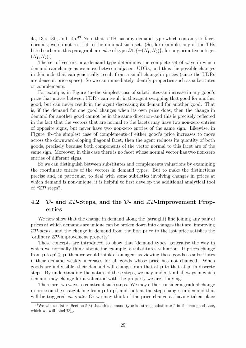
4a, 13a, 13b, and 14a.43 Note that a TH has any demand type which contains its facetnormals; we do not restrict to the minimal such set. (So, for example, any of the THslisted earlier in this paragraph are also of type D∪{±(N1, N2)}, for any primitive integer(N1, N2).)

The set of vectors in a demand type determines the complete set of ways in whichdemand can change as we move between adjacent UDRs, and thus the possible changesin demands that can generically result from a small change in prices (since the UDRsare dense in price space). So we can immediately identify properties such as substitutesor complements.

For example, in Figure 4a–the simplest case of substitutes–an increase in any good’sprice that moves between UDR’s can result in the agent swapping that good for anothergood, but can never result in the agent decreasing its demand for another good. Thatis, if the demand for one good changes when its own price does, then the change indemand for another good cannot be in the same direction–and this is precisely reflectedin the fact that the vectors that are normal to the facets may have two non-zero entriesof opposite signs, but never have two non-zero entries of the same sign. Likewise, inFigure 4b–the simplest case of complements–if either good’s price increases to moveacross the downward-sloping diagonal facet, then the agent reduces its quantity of bothgoods, precisely because both components of the vector normal to this facet are of thesame sign. Moreover, in this case there is no facet whose normal vector has two non-zeroentries of different signs.

So we can distinguish between substitutes and complements valuations by examiningthe coordinate entries of the vectors in demand types. But to make the distinctionsprecise and, in particular, to deal with some subtleties involving changes in prices atwhich demand is non-unique, it is helpful to first develop the additional analytical toolof “ZD steps”.

4.2 D- and ZD-Steps, and the D- and ZD-Improvement Prop-erties

We now show that the change in demand along the (straight) line joining any pair ofprices at which demands are unique can be broken down into changes that are ‘improvingZD-steps ’, and the change in demand from the first price to the last price satisfies the‘ordinary ZD-improvement property’.

These concepts are introduced to show that ‘demand types’ generalise the way inwhich we normally think about, for example, a substitutes valuation. If prices changefrom p to p′ ≥ p, then we would think of an agent as viewing these goods as substitutesif their demand weakly increases for all goods whose price has not changed. Whengoods are indivisible, their demand will change from that at p to that at p′ in discretesteps. By understanding the nature of these steps, we may understand all ways in whichdemand may change for a valuation with the property we are studying.

There are two ways to construct such steps. We may either consider a gradual changein price on the straight line from p to p′, and look at the step changes in demand thatwill be triggered en route. Or we may think of the price change as having taken place

43We will see later (Section 5.3) that this demand type is “strong substitutes” in the two-good case,which we will label D2

ss.

29

all in one go, but that the agent is incrementally swapping bundles for ones that arepreferred at the new and final prices. In either case, if the agent sees goods as (forexample) ‘substitutes’, we expect this property to be evident at every one of the steps(just as, with divisible demand, the corresponding property is true at all prices).

By treating such steps as our primitives, we can build up a more general understand-ing of the economic nature of valuations for goods, be they substitutes, complements,or some combination.

By ‘ZD-steps ’, then, we mean a sequence of bundles demanded on the straight linebetween p and p′ such that the differences between consecutive bundles in this sequenceare vectors inD or integer multiples thereof (we denote these vectors as ZD := {wv | w ∈Z,v ∈ D}); by ‘improving’, we mean that the bundle at the end of each step is preferredto the bundle at the beginning of each step, at the final price vector.

It follows immediately that any valuation of any demand type D must satisfy aproperty we will call the ‘ordinary ZD-improvement property ’: given any starting bun-dle, x, which is the unique demand at some price, p, and any price p′ at which x is notdemanded, there exists a bundle x′′ which is strictly preferred to x at p′, and such thatx′′ − x ∈ ZD.44

This property is closely connected to Gul and Stacchetti’s (1999) result that a specificset of valuations satisfies their “single improvement property”.45 This holds if, givenany starting bundle, x, and any price p′ at which x is not demanded, there exists abundle x′′ which is strictly preferred to x at p′, and such that x′′ − x is a vector whoseentries include include at most one +1, at most one −1, and all others zero. Since theordinary ZD-improvement property applies only to “starting bundles”, x, correspondingto UDR prices, it is not a strict generalisation of the “single improvement property”which applies to all starting bundles for those valuations for which it holds. However,we will introduce a refinement of our property which strictly generalises the “singleimprovement property”, and so allows strict generalisations of Gul and Stacchetti’s(1999) results, in Section 5.

The importance of our definitions and results is that we can use them to show howour “demand types” correspond precisely to interesting properties of demand such aswhether agents view goods as substitutes or complements; see Subsections 4.3.1 and4.3.2.

We proceed by first giving a formal definition of improving ZD-steps that is easilyshown to be equivalent to the informal definition given above (see the discussion ofTheorem 4.4), and will be easier to work with. Specifically we will require that animproving ZD-step is a ZD-step which “satisfies the strict law of demand” with respectto the overall price change:46

44It obviously suffices to let x′′ be the bundle at the end of the first of any set of improving ZD-stepsinto which the demand change is broken down. Note, however, that the way we define our ‘ordinaryZD-improvement property’ does not require that x′′ be demanded at some price on the straight linebetween p and p′. We do this for consistency with Gul and Stacchetti’s (1999) related definition (seebelow). But the stronger concept of a ZD-step will be easier to use to characterise properties thatvaluations may have.

45Gul and Stacchetti (1999) restrict their attention to A = {0, 1}n. We will see later (Section 5.3)that this set of valuations corresponds to our concave demand type Dnss.

46That is, for an overall price change from p to p′, and a demand step from x to ˜x, we require

(p′ − p).(˜x− x) < 0, with the exception that the change in demand is, of course, zero if p and p′ are

30

Definition 4.2. For prices p and p′ such that Du(p) 6= Du(p′), we say we can break

down the demand change from p to p′ into ZD-steps if for all x ∈ Du(p) there existsx′ ∈ Du(p

′), and a series of bundles x = x0, . . . ,xl = x′, demanded respectively at prices(1−λj)p+λjp

′, j = 0, . . . , l, for some 0 = λ0 ≤ · · · ≤ λl = 1, such that xj−xj−1 ∈ ZD.We call these ZD-steps improving if each demand change additionally “satisfies the

strict law of demand” with respect to the whole price change, that is, (p′ − p).(xj −xj−1) < 0.

We say we can break down the demand change into improving D-steps if there alwaysexists x0, . . . ,xl = x′ ∈ Du(p

′) satisfying these conditions and xj − xj−1 ∈ D for all j.

Definition 4.3. We say a valuation u satisfies the ordinary ZD-improvement propertyif, for any bundle x which is the unique demand at some price, p, i.e., satisfying Du(p) ={x}, and any price p′ such that x /∈ Du(p

′), there exists x′′ which is strictly preferredto x at price p′, and such that x′′ − x ∈ ZD.

We say the valuation u satisfies the ordinary D-improvement property if there alwaysexists x′′ which is strictly preferred to x at p′ and x′′ − x ∈ D.

Theorem 4.4. If D is any demand type, the following are equivalent for a valuationu:

1. u is of demand type D;

2. for any p such that #Du(p) = 1 and any p′ we can break down the demand changefrom p to p′ in improving ZD-steps;

3. for any p such that #Du(p) = 1, and any i ∈ {1, . . . , n} and any ε > 0, we canbreak down the demand change from p to p + εei in ZD-steps;

4. u satisfies the ordinary ZD-improvement property.

Proof. See Appendix A.1. �

Condition 2 implies 4 straightforwardly, because the fact that each separate stepsatisfies the “strict law of demand” with respect to the overall price change, means thateach successive bundle in the sequence must be strictly preferred to its predecessor atthe final price. So, in particular, the second bundle in the sequence is a bundle thatis strictly preferred to the starting bundle at the final price. Condition 4 implies 1because the only bundles preferred to a bundle demanded in a UDR, at any price thatis just on the other side of any facet bounding the UDR, are demanded on the facetitself, so the ordinary ZD-improvement property implies that the primitive integer facetnormal must lie in D. Condition 2 clearly implies 3, and 3 implies 1 because any facetwhose normal was not in D would not satisfy property 3 for some good i. Finally,the relationship between 1 and 2 is straightforward for any pair of prices at which thedemands are unique, and for which the straight line joining them crosses only facetinteriors, although it needs more careful argument when the price path crosses lowerdimensional cells of the TH.

within the same UDR. (The strict law of demand generalises the observation that demand must godown for goods whose prices go up–see e.g. Mas-Colell et al., 1995, Proposition 2.F.1.)

31

The inclusion of 3 shows that studying demand changes arising from a change ina single price suffices to understand the shapes of the trade-offs an agent might makeand, moreover, that we need not assume the ‘improving’ property, since this will holdautomatically.

It is, however, very useful to know that we can always choose ‘improving’ ZD-steps,since this greatly restricts the range of possible steps for any price change. We will seethis when we prove the relationships between certain demand types and the concepts ofsubstitutes and complements (see Propositions 4.8 and 4.11).

The reason we need ZD-steps, rather than onlyD-steps, is because of possible failuresof concavity–consider, for example, the function of one variable v(0) = v(1) = 0, v(2) = 2for which demand jumps from zero to 2 as price rises above 1. If we additionally assumethat u is concave throughout, we can strengthen Theorem 4.4 to deal with improvingD-steps and the ordinary D-improvement property:

Theorem 4.5. If D is any concave demand type, the following are equivalent for aconcave valuation u:

1. u is of (concave) demand type D;

2. for any p such that #Du(p) = 1 and any p′ we can break down the demand changefrom p to p′ in improving D-steps;

3. for any p such that #Du(p) = 1, and any i ∈ {1, . . . , n} and any ε > 0, we canbreak down the demand change from p to p + εei in improving D-steps;

4. u satisfies the ordinary D-improvement property.

Proof. See Appendix A.1. �

On the other hand, we might ask whether concavity need be explicitly assumed in2, 3 and 4. However, Example A.1 in the appendix shows the fact that we can alwaysbreak down the demand change between any UDR prices in improving D-steps does notimply u is concave, so we must assume concavity for 2 and 3. Similarly, Example A.2shows that the ordinary D-improvement property on its own does not imply concavity.Thus Theorem 4.5 is indeed stated in its most general form.

We now illustrate the application of improving ZD-steps, and Theorem 4.4, in thecases of ‘ordinary’ substitutes and complements:

4.3 Examples

4.3.1 Ordinary Substitutes

We use the standard definitions of “(ordinary) substitutes” as in Ausubel and Mil-grom (2002).47 An appealing aspect of this definition is that, as they show (their The-orem 10), it is equivalent to the submodularity of the dual profit function.

47That is, we call “ordinary substitutes”, precisely what Ausubel and Milgrom (2002) simply call“substitutes”. We hope this increases clarity (since others loosely refer to substitutes in other ways).Note, in particular, that Ausubel and Milgrom’s (2002) definition (our Definition 4.6) is not identical tothat of Kelso and Crawford (1982) when there are multiple units of three or more goods. (See Danilovet al. 2003 Example 6 and Theorem 1); the definitions are equivalent in the simpler cases n = 2 (see

32

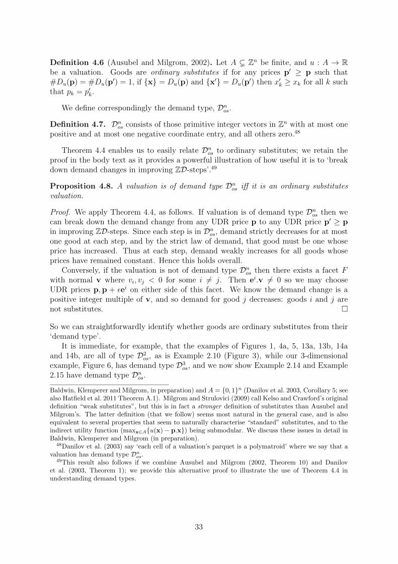
Definition 4.6 (Ausubel and Milgrom, 2002). Let A ( Zn be finite, and u : A → Rbe a valuation. Goods are ordinary substitutes if for any prices p′ ≥ p such that#Du(p) = #Du(p

′) = 1, if {x} = Du(p) and {x′} = Du(p′) then x′k ≥ xk for all k such

that pk = p′k.

We define correspondingly the demand type, Dnos.

Definition 4.7. Dnos consists of those primitive integer vectors in Zn with at most onepositive and at most one negative coordinate entry, and all others zero.48

Theorem 4.4 enables us to easily relate Dnos to ordinary substitutes; we retain theproof in the body text as it provides a powerful illustration of how useful it is to ‘breakdown demand changes in improving ZD-steps’.49

Proposition 4.8. A valuation is of demand type Dnos iff it is an ordinary substitutesvaluation.

Proof. We apply Theorem 4.4, as follows. If valuation is of demand type Dnos then wecan break down the demand change from any UDR price p to any UDR price p′ ≥ pin improving ZD-steps. Since each step is in Dnos, demand strictly decreases for at mostone good at each step, and by the strict law of demand, that good must be one whoseprice has increased. Thus at each step, demand weakly increases for all goods whoseprices have remained constant. Hence this holds overall.

Conversely, if the valuation is not of demand type Dnos then there exists a facet Fwith normal v where vi, vj < 0 for some i 6= j. Then ei.v 6= 0 so we may chooseUDR prices p,p + εei on either side of this facet. We know the demand change is apositive integer multiple of v, and so demand for good j decreases: goods i and j arenot substitutes. �

So we can straightforwardly identify whether goods are ordinary substitutes from their‘demand type’.

It is immediate, for example, that the examples of Figures 1, 4a, 5, 13a, 13b, 14aand 14b, are all of type D2

os, as is Example 2.10 (Figure 3), while our 3-dimensionalexample, Figure 6, has demand type D3

os, and we now show Example 2.14 and Example2.15 have demand type Dnos.

Baldwin, Klemperer and Milgrom, in preparation) and A = {0, 1}n (Danilov et al. 2003, Corollary 5; seealso Hatfield et al. 2011 Theorem A.1). Milgrom and Strulovici (2009) call Kelso and Crawford’s originaldefinition “weak substitutes”, but this is in fact a stronger definition of substitutes than Ausubel andMilgrom’s. The latter definition (that we follow) seems most natural in the general case, and is alsoequivalent to several properties that seem to naturally characterise “standard” substitutes, and to theindirect utility function (maxx∈A{u(x)− p.x}) being submodular. We discuss these issues in detail inBaldwin, Klemperer and Milgrom (in preparation).

48Danilov et al. (2003) say ‘each cell of a valuation’s parquet is a polymatroid’ where we say that avaluation has demand type Dnos.

49This result also follows if we combine Ausubel and Milgrom (2002, Theorem 10) and Danilovet al. (2003, Theorem 1); we provide this alternative proof to illustrate the use of Theorem 4.4 inunderstanding demand types.

33

Example 2.14 revisited. Because the valuations of the ‘workers’ in Kelso and Craw-ford’s (1982) matching model have domain {0,−e(i,j) | j = 1, . . . ,m2}, their only possibleSNP edges are in Dnos, so they are of demand type Dnos. Since the ‘firms’ in this modelhave valuations with domain {0, 1}m1 which are assumed to satisfy the conditions forordinary substitutes, they are also of demand type Dnos.

Example 2.15 revisited. Hatfield et al. (2013) describe the goods to be sold in theirmodel as complements of goods to be bought, because they measure both buying andselling as non-negative quantities. But if we instead think of selling as just “negativebuying” then the “complementarities” in their model disappear, and it is then clear thattheir condition of ‘full substitutability’ is precisely the ordinary substitutes conditionof, e.g., Ausubel and Milgrom (2002). That is, an agent whose valuation domain is asdescribed in Example 2.15 has ‘fully substitutable’ preferences iff the valuation is of typeDnos.50

Example 2.12 illustrates a special case of this model: the agent regards the actions ofbuying good 2 and selling good 1 as complements, but regards the buying of both goods(possibly in negative quantities) as substitutes. The point is easily seen geometrically–Figure 5 clearly represents substitutes preferences, and not the complements preferencesof Figure 4b, which we formally introduce in Section 4.3.2.

4.3.2 Ordinary Complements

“Complements” can be defined analogously to the Definition 4.6 of “ordinary sub-stitutes”:

Definition 4.9. Let A ( Zn be finite, and let u : A → R be a valuation. Goods areordinary complements if, for any prices p′ ≥ p such that #Du(p) = #Du(p

′) = 1, if{x} = Du(p) and {x′} = Du(p

′) then x′k ≤ xk for all k such that pk = p′k.

Similarly to Definition 4.7 we define a corresponding demand type:

Definition 4.10. Dnoc consists of those primitive integer vectors in Zn whose non-zerocoordinate entries are all of the same sign.

As in Proposition 4.8, it is an elementary consequence of Theorem 4.4 that

Proposition 4.11. A valuation is of demand type Dnoc iff it is an ordinary complementsvaluation.

Proof. As with Proposition 4.8, this follows immediately from Theorem 4.4: we breakdown the change in demand from some UDR price p to p′ ≥ p into improving ZD-steps.As before, at each step demand must strictly decrease for at least one good whose pricehas increased; this time, the nature of Dnoc implies that demand weakly decreases for

50The precise ‘choice language’ definition of Hatfield et al. (2013) is superficially different from ourDefinition 4.6, but an earlier version of their paper presents an alternative ‘demand-language’ definition(Hatfield et al., 2011, Definition 4) which corresponds precisely to the Ausubel and Milgrom (2002)definition, and moreover they confirm (Hatfield et al., 2011, Theorem A.1) that this definition is equiv-alent to the ‘choice-language’ definition of Hatfield et al. (2013). They define “full substitutability”using Sun and Yang’s (2006) ‘gross substitutes and complements’ ideas; see Section 5.5.

34

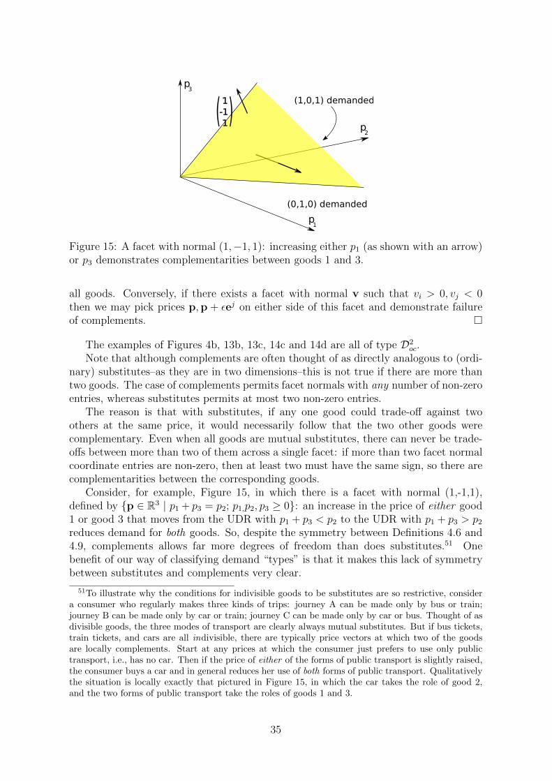
p3

(0,1,0) demanded

(1,0,1) demanded 1-1 1)

)

p1

p2

Figure 15: A facet with normal (1,−1, 1): increasing either p1 (as shown with an arrow)or p3 demonstrates complementarities between goods 1 and 3.

all goods. Conversely, if there exists a facet with normal v such that vi > 0, vj < 0then we may pick prices p,p + εej on either side of this facet and demonstrate failureof complements. �

The examples of Figures 4b, 13b, 13c, 14c and 14d are all of type D2oc.

Note that although complements are often thought of as directly analogous to (ordi-nary) substitutes–as they are in two dimensions–this is not true if there are more thantwo goods. The case of complements permits facet normals with any number of non-zeroentries, whereas substitutes permits at most two non-zero entries.

The reason is that with substitutes, if any one good could trade-off against twoothers at the same price, it would necessarily follow that the two other goods werecomplementary. Even when all goods are mutual substitutes, there can never be trade-offs between more than two of them across a single facet: if more than two facet normalcoordinate entries are non-zero, then at least two must have the same sign, so there arecomplementarities between the corresponding goods.

Consider, for example, Figure 15, in which there is a facet with normal (1,-1,1),defined by {p ∈ R3 | p1 + p3 = p2; p1,p2, p3 ≥ 0}: an increase in the price of either good1 or good 3 that moves from the UDR with p1 + p3 < p2 to the UDR with p1 + p3 > p2

reduces demand for both goods. So, despite the symmetry between Definitions 4.6 and4.9, complements allows far more degrees of freedom than does substitutes.51 Onebenefit of our way of classifying demand “types” is that it makes this lack of symmetrybetween substitutes and complements very clear.

51To illustrate why the conditions for indivisible goods to be substitutes are so restrictive, considera consumer who regularly makes three kinds of trips: journey A can be made only by bus or train;journey B can be made only by car or train; journey C can be made only by car or bus. Thought of asdivisible goods, the three modes of transport are clearly always mutual substitutes. But if bus tickets,train tickets, and cars are all indivisible, there are typically price vectors at which two of the goodsare locally complements. Start at any prices at which the consumer just prefers to use only publictransport, i.e., has no car. Then if the price of either of the forms of public transport is slightly raised,the consumer buys a car and in general reduces her use of both forms of public transport. Qualitativelythe situation is locally exactly that pictured in Figure 15, in which the car takes the role of good 2,and the two forms of public transport take the roles of goods 1 and 3.

35

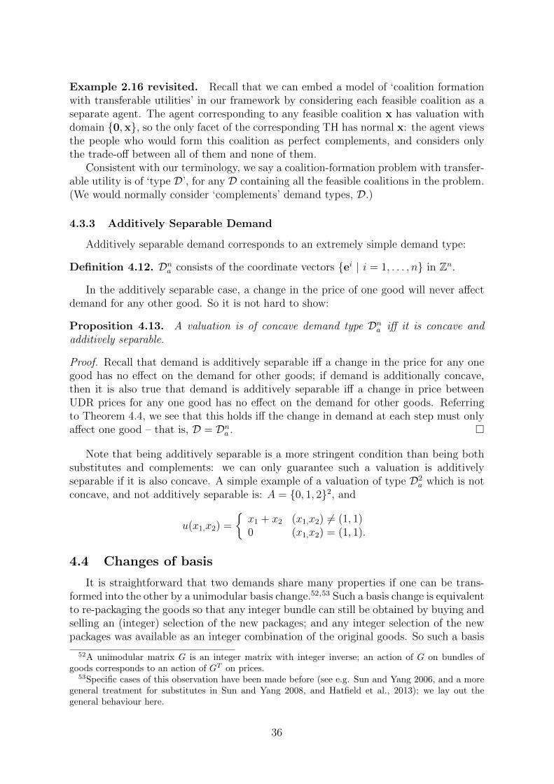
Example 2.16 revisited. Recall that we can embed a model of ‘coalition formationwith transferable utilities’ in our framework by considering each feasible coalition as aseparate agent. The agent corresponding to any feasible coalition x has valuation withdomain {0,x}, so the only facet of the corresponding TH has normal x: the agent viewsthe people who would form this coalition as perfect complements, and considers onlythe trade-off between all of them and none of them.

Consistent with our terminology, we say a coalition-formation problem with transfer-able utility is of ‘type D’, for any D containing all the feasible coalitions in the problem.(We would normally consider ‘complements’ demand types, D.)

4.3.3 Additively Separable Demand

Additively separable demand corresponds to an extremely simple demand type:

Definition 4.12. Dna consists of the coordinate vectors {ei | i = 1, . . . , n} in Zn.

In the additively separable case, a change in the price of one good will never affectdemand for any other good. So it is not hard to show:

Proposition 4.13. A valuation is of concave demand type Dna iff it is concave andadditively separable.

Proof. Recall that demand is additively separable iff a change in the price for any onegood has no effect on the demand for other goods; if demand is additionally concave,then it is also true that demand is additively separable iff a change in price betweenUDR prices for any one good has no effect on the demand for other goods. Referringto Theorem 4.4, we see that this holds iff the change in demand at each step must onlyaffect one good – that is, D = Dna . �

Note that being additively separable is a more stringent condition than being bothsubstitutes and complements: we can only guarantee such a valuation is additivelyseparable if it is also concave. A simple example of a valuation of type D2

a which is notconcave, and not additively separable is: A = {0, 1, 2}2, and

u(x1,x2) =

{x1 + x2 (x1,x2) 6= (1, 1)0 (x1,x2) = (1, 1).

4.4 Changes of basis

It is straightforward that two demands share many properties if one can be trans-formed into the other by a unimodular basis change.52,53 Such a basis change is equivalentto re-packaging the goods so that any integer bundle can still be obtained by buying andselling an (integer) selection of the new packages; and any integer selection of the newpackages was available as an integer combination of the original goods. So such a basis

52A unimodular matrix G is an integer matrix with integer inverse; an action of G on bundles ofgoods corresponds to an action of GT on prices.

53Specific cases of this observation have been made before (see e.g. Sun and Yang 2006, and a moregeneral treatment for substitutes in Sun and Yang 2008, and Hatfield et al., 2013); we lay out thegeneral behaviour here.

36

change leaves many important properties of demand–including, we will see in Section 6,the existence of competitive equilibrium–unaffected.

Likewise, such a basis change simply distorts the TH by a linear transformationwhich leaves its important structure unaffected:

Proposition 4.14 (cf. Gorman, 1976, p. 219-20). For A ( Zn and u : A → R anda unimodular n × n matrix G, define the (“pullback”) basis change of u by G to beG∗u : G−1A→ R via G∗u(y) := u(Gy). Then

1. A bundle is demanded under the original demand at a certain price iff an asso-ciated bundle is demanded under the transformed demand at an associated price;specifically: x ∈ Du(p) ⇐⇒ G−1x ∈ DG∗u(G

Tp).

2. The TH of the transformed demand is given by a linear transformation of theoriginal demand: TG∗u = {GTp | p ∈ Tu};

3. The inverse transformation to G applies to demand types: u(·) is of (concave)demand type D iff G∗u(·) is of (concave) demand type G−1D = {G−1v | v ∈ D}.

Proof. See Appendix A.1. �

As a simple example, if n = 2 then ordinary substitutes Dnos are a unimodular basis

change of ordinary complements Dnoc, via the matrix

(1 00 −1

).54 As discussed in

Section 4.3.2, this does not hold for n ≥ 3.

5 Complete Demand Types and Unimodular De-

mand Types

The previous section showed that the change in demand between any two UDRprices could be broken down into improving ZD-steps and, for concave valuations, intoimproving D-steps. Since UDR prices are dense in the set of all prices, this tells us agreat deal about the structure of demand.

However, one may wish for results relating to every possible price and starting bundle.For example, the standard definition of ‘ordinary substitutes’ for indivisible goods (see,e.g., Ausubel and Milgrom, 2002) that we use only considers demand changes betweenUDR prices, but others have used a definition of substitutes that compares demands atany pair of prices (see, for example, Kelso and Crawford 1982).55 As is shown by Danilovet al. (2003, Example 6), for n ≥ 3 there exist valuations which satisfy the ‘ordinary

54So, for example, we will see that with two goods (in indivisible units), competitive equilibrium fails“as often” for sets of agents with ordinary substitutes demands, as for sets of agents with ordinarycomplements demands, even though the economic properties of substitutes and complements are, ofcourse, very different.

55These two definitions are equivalent when A = {0, 1}n (see Corollary 5.17) and almost all pre-ceding work has been restricted to this case, so the distinction between these definitions is sometimesblurred. We discuss the relationships between alternative definitions of substitutes at length in Baldwin,Klemperer and Milgrom (in preparation).

37

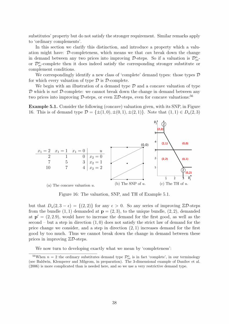
substitutes’ property but do not satisfy the stronger requirement. Similar remarks applyto ‘ordinary complements’.

In this section we clarify this distinction, and introduce a property which a valu-ation might have: D-completeness, which means we that can break down the changein demand between any two prices into improving D-steps. So if a valuation is Dnos-or Dnoc-complete then it does indeed satisfy the corresponding stronger substitute orcomplement conditions.

We correspondingly identify a new class of ‘complete’ demand types: those types Dfor which every valuation of type D is D-complete.

We begin with an illustration of a demand type D and a concave valuation of typeD which is not D-complete: we cannot break down the change in demand between anytwo prices into improving D-steps, or even ZD-steps, even for concave valuations:56

Example 5.1. Consider the following (concave) valuation given, with its SNP, in Figure16. This is of demand type D = {±(1, 0),±(0, 1),±(2, 1)}. Note that (1, 1) ∈ Du(2, 3)

x1 = 2 x1 = 1 x1 = 0 u2 1 0 x2 = 07 5 3 x2 = 1

10 7 4 x2 = 2

(a) The concave valuation u.

(0,0)

(b) The SNP of u.

p1

p2

1 2 3

1

2

3

4

5

2

2

(0,0)

(2,0)

(0,1)

(0,2)

(2,1)

(2,2)

(c) The TH of u.

Figure 16: The valuation, SNP, and TH of Example 5.1.

but that Du(2, 3 − ε) = {(2, 2)} for any ε > 0. So any series of improving ZD-stepsfrom the bundle (1, 1) demanded at p = (2, 3), to the unique bundle, (2, 2), demandedat p′ = (2, 2.9), would have to increase the demand for the first good, as well as thesecond – but a step in direction (1, 0) does not satisfy the strict law of demand for theprice change we consider, and a step in direction (2, 1) increases demand for the firstgood by too much. Thus we cannot break down the change in demand between theseprices in improving ZD-steps.

We now turn to developing exactly what we mean by ‘completeness’:

56When n = 2 the ordinary substitutes demand type Dnos is in fact ‘complete’, in our terminology(see Baldwin, Klemperer and Milgrom, in preparation). The 3-dimensional example of Danilov et al.(2006) is more complicated than is needed here, and so we use a very restrictive demand type.

38

5.1 Completeness of a Demand Type

Recall that Definition 4.3 was not exactly a generalisation of Gul and Stacchetti’s(1999) “single-improvement property”: a true generalisation may be given as follows:57

Definition 5.2. We say a valuation u satisfies the complete D-improvement propertyif, for any bundle x and for any price p′ such that x /∈ Du(p

′), there exists x′′ which isstrictly preferred to x at price p′ and such that x′′ − x ∈ D.

Note how this differs from Definition 4.3: for the ‘complete’ property we do not insistthat the bundle x be demanded at any price at all, whereas the ‘ordinary’ propertyrequires that x be demanded uniquely at some price.

We show that, given concavity, the complete D-improvement property is equivalentto our being able to break down any change in demand into improving D-steps:

Proposition 5.3. The following are equivalent for a concave valuation u of type D:

1. we can break down the demand change from any p to any p′ in improving D-steps;

2. u satisfies the complete D-improvement property.

Proof. See Appendix A.2. �

The assumption of concavity is needed to ensure that every bundle x is demanded atsome price – and hence that we can use improving D-steps to obtain D-improvements.58

Since concavity is also needed for the existence of improving D-steps and the ordinaryD-improvement property (as distinct from ZD-steps and the ordinary ZD-improvementproperty) we simply work under this assumption for this section.

Definition 5.4.

1. We say a concave valuation u is D-complete if the equivalent conditions of Propo-sition 5.3 hold.

2. We say a concave demand type D is a complete demand type if every concavevaluation of type D is D-complete.

It is straightforward now to provide the following analogue to Theorems 4.4 and 4.5:

Corollary 5.5. If D is any complete demand type, then the following are equivalent fora concave valuation u:

1. u is of concave demand type D (and the equivalent conditions of Theorem 4.4hold);

2. we can break down the demand change from any p to any p′ in improving D-steps;

57This also generalises Sun and Yang (2009), which generalised Gul and Stacchetti (1999) to the caseof “gross substitutes and complements”.

58In fact, 5.3.2⇒5.3.1 when u is not concave; one may see that the proof makes no use of concavity.However, a non-concave valuation satisfying 5.3.1 need not satisfy 5.3.2; consider Example 5.1 with themodification u(1, 1) = 4.

39

3. for any p and any i ∈ {1, . . . , n} and any ε > 0, we can break down the demandchange from p to p + εei in improving D-steps;

4. u satisfies the complete D-improvement property.

Proof. Given that D is complete, 1⇔2 and 1⇔4 by Proposition 5.3 and Definition 5.2.That 2⇒3 is clear; that 3⇒1 follows by the corresponding argument of Theorem 4.5. �

Thus, once completeness of a demand type is known, the weaker checks of Theorem4.4 are sufficient to provide their ‘complete’ counterparts given here. Moreover, as isintuitive, completeness is preserved under unimodular basis changes:

Proposition 5.6. Suppose G is a unimodular n× n matrix.

1. If u : A → R is concave and D-complete, then G∗u is concave and is G−1D-complete.

2. If D is complete then G−1D is complete.

Proof. See Appendix A.2. �

The question remains of which demand types are complete. In Section 5.2 we developa sufficient condition: unimodularity. However, this condition is not necessary. Here wegive two examples, one unimodular and one not.

Example 5.7. The set Dnall of all primitive integer n-vectors is complete. This istrivial: given any concave valuation and any prices p,p′ we can simply note the bundlesdemanded in improving steps on the straight line from p to p′, interpolating additionalprimitive integer steps if necessary. It is of interest to emphasise this point, becausemany sub-types D ( Dnall are not complete. This fact stands in contrast to the propertyof unimodularity, which we shall come to in Section 5.2.

Example 5.8. The set Dna of the coordinate vectors is a complete demand type. Asshown in Proposition 4.13, any concave valuation u of type Dna is additively separable.Thus, for any good i, the quantity demanded of any single good depends only on theprice for that good. So if x /∈ Du(p) for any bundle x and price vector p, then we mayadjust the quantities of all goods independently, towards the desired levels. That is, wemay make a series of Dna -improvements given any starting bundle and price.

5.2 Unimodularity: a sufficient condition for completeness

We now introduce a condition on demand types which is sufficient for their com-pleteness; strikingly, the same condition is also necessary and sufficient for existence ofcompetitive equilibrium (see Section 6.3).

Throughout, we write “the determinant of vectors w1, . . . ,wn” to mean the deter-minant of the n × n matrix which has these vectors as its columns.59 We say that alinearly independent set {w1, . . . ,ws} of vectors is “an integer basis for the subset theyspan” if, whenever y ∈ Zn can be written as

∑si=1 aiw

i, in which ai ∈ R, then in factai ∈ Z for i = 1, . . . , s.

59Changing the order of the vectors may change the sign of the determinant, so strictly speaking thedeterminant is a property of an ordered n-tuple of vectors. This detail does not concern us as we areonly ever interested in the absolute values of determinants.

40

(0,0)

Figure 17: The SNP of Example 5.1, with the relevant vectors highlighted.

Definition 5.9. We say a demand type D is unimodular if any linearly independent setof vectors in D is an integer basis for the subspace they span.

It is clear that the set Dnall of Example 5.7 does not have this property, whereas theset Dna of Example 5.8 does have it. We now clarify the implications of unimodularityby considering an example in which both unimodularity and completeness fail:

Example 5.1 revisited. Recall we considered a particular valuation u of demandtype D = {±(1, 0),±(0, 1),±(2, 1)}. This demand type is not unimodular. The vector(1, 1) is in the span of (0, 1) and (2, 1) but it is not possible to express it as an integercombination of these vectors. This impossibility is illustrated in Figure 17, in which thevectors (0, 1) and (2, 1), starting from the origin, are highlighted in red.

It is similarly impossible to move on from the bundle (1, 1) to the bundle (2, 2) usingthis pair of directions, as highlighted in blue. Since these two vectors are the onlytwo in D that change the quantity of Good 2 demanded, the failure of D-completenessfollows.60

To understand the relevance of unimodularity in general, consider a set of s linearlyindependent vectors from a demand type D. These are the edges of an s-dimensionalparallelepiped. This shape will contain no integer point (either in its boundary or in itsinterior) aside from its vertices, iff, our set of vectors is an integer basis for the subspacethey span. Thus the scenario of Figure 17, in which the bundle (1, 1) gives difficulties,simply cannot arise if the demand type is unimodular.

This condition may appear difficult to check. However, returning to the paral-lelepiped, it is not too difficult to see that unimodularity holds iff the s-dimensionalvolume of the parallelepiped is 1. When s = n, this volume is simply the (absolutevalue of the) determinant of the vectors along its edges. When s < n, unimodularity isequivalent to the ability to add additional integer vectors that build the s-dimensionalvolume out into an n-dimensional volume of 1, i.e., so that the determinant is again ±1.(In the case of Figure 17, the determinant in question is 2).

We gather these conditions with an alternative check for unimodularity when s < n,via appropriate determinants of submatrices, as follows:

60If (1, 1) were in the demand type, then it would be possible to make a suitable step, confirming (asis already clear from Example 5.7) that unimodularity is not necessary.

41

Remark 5.10. The following are equivalent, for a set of s linearly independent vectorsin Zn:

1. they are an integer basis for the subspace they span;

2. A s-dimensional parallelepiped in Rn with vertices in Zn and these vectors as edgescontains no point in Zn except its vertices;

3. they can be extended to a basis for Rn, of integer vectors, with determinant ±1;

4. among the determinants of all the s× s matrices consisting of s rows of the n× smatrix whose columns are these s vectors, the greatest common factor is 1.

Proofs of these facts may be found in Cassels (1959).61 Note that when s = n then both2 and 3 remind us that the determinant of the vectors is ±1. We refer to a set of vectorsas unimodular if every linearly independent subset has these properties.

Our result is now:

Theorem 5.11. If a concave demand type is unimodular, then it is complete.

Proof. See Appendix A.2.62 �

Using Remark 5.10.3 we can state a slightly weaker result that is more intuitive andvery easy to check:

Corollary 5.12. With n goods, a concave demand type D = {v1, . . . ,vr}, in whichv1, . . . ,vr span Rn, is complete if every subset of n vectors from D has determinant 0or ±1.

The intuition for Theorem 5.11 is as described above regarding Figure 17. Moredetail is required because not every SNP-face is a parallelepiped, and general SNP facesmay contain non-vertex points, even for a unimodular demand type. However, we showthat, when unimodularity holds, we may step from a non-vertex point to another point inthe SNP face, in the direction of a vector in D. The additional assumption of concavityis required to ensure that this new point in the SNP face is indeed demanded at relevantprices; see Example A.3 for an example of what happens when it fails.

We will see below that a very nice example of a concave unimodular demand typeis ‘strong substitutes’. The relationship between this and the corresponding ‘single’improvement property is well known (Gul and Stacchetti, 1999; Milgrom and Strulovici,

611 ⇔ 3 follows from Cassels (1959) Lemma I.1 and Corollary I.3. 1 ⇔ 4 is Cassels (1959) LemmaI.2. For 1 ⇔ 2 consider a parallelepiped P whose vertices are y +

∑si=1 aiw

i for ai ∈ {0, 1}. If z is anon-vertex integer point in P , then z−y exhibits the failure of 1. Conversely, if failure of 1 is exhibitedby an integer

∑si=1 biw

i where bi are not all integers, then y +∑si=1 aiw

i exhibits failure of 2, whereai is the non-integer part of bi in each case.

62As shown there, in fact we prove a stronger result: we need only assume that, for any vectors V ⊆ D,there exist linearly independent vectors w1, . . . ,ws ∈ D, whose span over R coincides with the span overR of V and such that, for any v1, . . . ,vs−1 ∈ V and any i = 1, . . . , s, the vectors v1, . . . ,vs−1,wi areeither linearly dependent or are a unimodular set. This property is clearly implied by unimodularityof D, as we may take the set w1 . . . ,ws to be any linearly independent and spanning subset of V.However, it is not sufficient for unimodularity; the set D = ±{0, 1}3 is not unimodular but does havethis property.

42

2009). Corollary 5.5 and Theorem 5.11 together strictly generalise this result by showingthat the complete D-improvement property is satisfied by all valuations of type D for anyunimodular concave demand type D.63 It follows from Seymour (1980) that there aremany such demand types that are not a unimodular basis change of strong substitutes.

5.3 Unimodular Demand Types for Substitute Goods

Following from Theorem 5.11 and the arguments of Section 4.3.1 it is clear that avaluation will satisfy the following definition of substitutes if it is Dnos-complete:

Proposition 5.13. If a concave valuation u is Dnos-complete then, for any prices p′ ≥ pand any x ∈ Du(p), there exists x′ ∈ Du(p

′) such that x′k ≥ xk for all k such thatp′k = pk.

Proof. One may make use of Dnos-steps exactly as in Proposition 4.8, but now startingat any price p. �

Note that the latter condition is provided as the definition of indivisible substitutes byKelso and Crawford (1982).64

Following Theorem 5.11, then, we see:

Proposition 5.14. If D ( Dnos is unimodular then every concave valuation of type Dis a Dnos-complete valuation (and so satisfies the Kelso-Crawford definition).

On the other hand, for ordinary substitutes the Dnos-complete property may fail: seeDanilov et al. (2003, Example 6).65 Note also that, in order to apply the proposition, thedemand type with respect to which u is complete must itself be a subset of Dnos; since(as just noted) there are ordinary substitutes which are not Dnos-complete, and sinceevery valuation is of the complete demand type Dnall (see Example 5.7), there clearlyexist ordinary substitute valuations that are D-complete for some D 6⊆ Dnos, but are notDnos-complete.

We refer to unimodular demand types D ( Dnos as ‘unimodular substitute’ demandtypes.

One example of a ‘unimodular substitute’ demand type is {±(−1, 1),±(−1, 2),±(0, 1)}.Note that this demand type does not contain both distinct coordinate vectors – an agentcannot be indifferent about whether to buy or sell an additional unit of good 1, whilemaintaining constant demand for good 2. But this is still a natural model if, for exam-ple, agents are manufacturers, selling good 1, which they can manufacture from different

63It is also observed by Danilov et al. (2008, 2013) that ‘interval concave functions’ can equivalentlybe characterised by ‘interval package improvements’ – see our Example 5.24. However, as demonstratedin Example 5.24, the interval package demand type is a unimodular basis change of the strong substitutedemand type, and so their result follows immediately from the Gul and Stacchetti result.

64There are various nomenclatures in use for this concept; Danilov et al. (2003) call them ‘grosssubstitutes’ following Kelso and Crawford (who strictly speaking deal only with the {0, 1}n case);Milgrom and Strulovici (2009) call them ‘weak substitutes’.

65Thus, Ausubel and Milgrom’s (2002) definition (our Definition 4.6) is not identical to that ofKelso and Crawford (1982) when there are multiple units of three or more goods. The definitionsare equivalent in the simpler cases n = 2 (see Baldwin, Klemperer and Milgrom, in preparation) andA = {0, 1}n (Danilov et al. 2003, Corollary 5; see also Hatfield et al. 2011 Theorem A.1). See Baldwin,Klemperer and Milgrom (in preparation) for further discussion.

43

quantities of good 2, depending perhaps on the technology in use–indeed this is the nat-ural generalisation of Hatfield et al. (2013) to multiple units of goods, see Examples 2.12and 2.15.

The best-known example of a unimodular set of vectors also gives rise to a substitutedemand type:

Definition 5.15. Dnss consists of those vectors in Zn with at most one +1 and at mostone −1 coordinate entry, and all others zero.66

Checking that this is a unimodular demand type is an application of a well-knownresult:

Theorem 5.16. Dnss is a unimodular demand type, and is maximal: if Dnss ( D thenD is not unimodular.

Proof. That the set of vectors that Dnss comprises is unimodular was first shown byPoincare (1900); an attractive inductive proof was provided by Veblen and Franklin(1921), which we reproduce in Appendix A.2. Its maximality is easy to show. If avector w were introduced with |wj| > 1 for some j then the determinant of w with all ei

such that i 6= j is wj, contradicting unimodularity by assumption. If a vector w has two+1 coordinate entries, say in i and j, then the determinant of it with ei − ej and all ek

such that k 6= i, j, has absolute value 2. Thus no additional vectors may be introducedwithout contradicting unimodularity. �

From the unimodularity of Dnss immediately follows:

Corollary 5.17. 67 A concave ordinary substitute valuation with domain A = {0, 1}nis a Dnos-complete valuation.

Proof. By Proposition 4.8 such a valuation is of demand type Dnos. If A = {0, 1}n thenthe only possible SNP edges in Dnos, and hence the only possible facet normals, are thosein Dnss. �

The vectors in Dnss were first related to substitutes by Tomizawa (1983), but withoutproof; proofs were offered by Danilov et al. (2003), and Fujishige and Yang (2003). Anequivalent formulation was given by Milgrom and Strulovici (2009), who also show thatthere are several additional equivalent characterisations. Here we gather several relevantdefinitions:

Definition 5.18.

1. A valuation u is a step-wise gross substitute valuation if for any p ∈ Rn, anyx ∈ Du(p) and any i ∈ {0, . . . , n}, either x ∈ Du(p + εei) for all ε ≥ 0 or thereexists ε ≥ 0 and x′ ∈ Du(p + εei) such that x′i = xi − 1 and x′−i ≥ x−i.

68

66Danilov et al. (2003) say a valuation is a ‘PM-function’ (where PM stands for polymatroid) in thiscase.

67An analogous result is Danilov et al. (2003) Corollary 5.68See Danilov et al. (2003).

44

2. A valuation u is a strong substitute valuation if, when we consider every unit ofevery good as a separate good, then they are ordinary substitutes.69

3. A valuation u satisfies the ordinary (complete) law of aggregate demand if fork ∈ {1, . . . , n}, any ε > 0 any p ∈ Rn and any x ∈ Zn such that {x} = Du(p)(resp. x ∈ Du(p)) there exists x′ ∈ Du(p + εek) such that

∑i x′i ≤

∑i xi.

70

4. A valuation u satisfies the consecutive integer property if, for every p ∈ Rn andevery i ∈ {1, . . . , n}, the set {xi | x ∈ Du(p)} consists of consecutive integers.71

Demand types provide nice ways to characterise the “law of aggregate demand” andthe consecutive integer property, and these characterisations in turn make it much easierto demonstrate alternative characterisations of strong substitutes than is possible usingtraditional techniques. It is both intuitively clear and straightforward that (details arein Appendix A.2):

Lemma 5.19.

1. A valuation u satisfies the ordinary (complete) law of aggregate demand iff it is ofsome (unimodular concave) demand type D such that, for all v ∈ D, either v ≥ 0,−v ≥ 0, or

∑ni=1 vi = 0.

2. A concave valuation u satisfies the consecutive integer property iff it is of someconcave demand type D ⊆ {−1, 0, 1}n.

It is then easy to use this Lemma to show the following, which slightly generalisesMilgrom and Strulovici (2009, Theorem 13):72

Corollary 5.20. For a valuation u, the following are equivalent:

1. u is of concave demand type Dnss;

2. u is a strong substitute valuation;

3. u is a concave step-wise gross substitute valuation;

4. u is concave and satisfies the complete Dnss-improvement property;

5. u is a concave ordinary substitute valuation and satisfies the ordinary law of ag-gregate demand;

6. u is a concave ordinary substitute valuation and satisfies the consecutive integerproperty;

69See Milgrom and Strulovici (2009). Note that, by Corollary 5.17, it is equivalent whether we definestrong substitutes as all units of all goods being Dnos-complete substitutes, or just as all units of allgoods being ordinary substitutes.

70See Hatfield and Milgrom (2005) for the ‘complete’ version.71See Milgrom and Strulovici (2009).72Milgrom and Strulovici (2009, Theorem 13) does not mention step-wise gross substitutes and as-

sumes the Dnos-complete property in 5 and 6.

45

Proof. 1⇔4 is an application of Theorem 5.11. The complete Dnss-improvement propertyis precisely the single-improvement property of Gul and Stacchetti (1999), so 4⇔2 followsfrom Milgrom and Strulovici (2009, Theorem 13).73 That 1⇔3 is clear from Corollary5.5.1⇔3 (and also given by Danilov et al. 2003, Proposition 7). That 1⇔5 follows sinceby Proposition 4.8 we know ordinary substitutes to be equivalent to demand type Dnosand since by Lemma 5.19.1, for the ordinary law of aggregate demand to additionallyhold, the only vectors in Dnos we can allow are those in Dnss. That 1⇔6 similarly followsfrom Lemma 5.19.2 since the vectors in Dnos satisfying the consecutive integer propertyare precisely the vectors of Dnss. �

We will in general refer to the valuations satisfying these equivalent conditions as‘strong substitutes’ as this terminology appears to have become more widely used (andis briefer than ‘concave step-wise gross substitutes’). We can now quickly and easilyidentify such valuations. It is immediate, for example, that the examples of Figures 1,4a, 5, 13a, 13b, and 14a are all of type D2

ss, while our 3-dimensional example, Figure6, has demand type D3

ss. However, Example 2.10 (Figure 3) has a facet with normal(−1, 2) (the line segment between the prices (4,3) and (6,4)), in addition to facets withnormals (1, 0), (0, 1), and (1,−1), and so is not of type D2

ss, but is of type D2os, as is the

example of Figure 14b.74

Examples 2.14 and 2.15 revisited again. Recall we saw in Section 4.3.1 that themodels of Kelso and Crawford (1982) and Hatfield et al. (2013) could be understood asordinary substitute demand types. Now note that they are both also of demand typeDnss. In the case of Kelso and Crawford (1982), all workers and all firms have valuationswith domain contained in {0, 1}m1+m2 . In the case of Hatfield et al. (2013), since eachagent is restricted to either selling or buying any individual good, a re-ordering of goodsshows their valuation has domain a subset of {0, 1}n1 ×{−1, 0}n2 for some non-negativen1 + n2 = n.75 Thus, following the same arguments as Corollary 5.17, every SNP edge,and so every facet normal, must be in Dnss: the structure of preferences is again strongsubstitutes.

5.4 Unimodular Demand Types for Complementary Goods

Preferences for complementary goods are less thoroughly treated in the literaturethan preferences for substitutes, but we can use our techniques, and the analogy betweenthe two cases, to develop some results for complements:

73Strictly speaking, the proof of Milgrom and Strulovici (2009, Theorem 13) is incomplete, as theconnection between the single-improvement property and the strong substitute property relies on theirTheorem 2, whose proof is incomplete. However, Danilov et al. (2003, Corollary 5) provide the missingpiece.

In the case that n = 1, the result that 1⇔2 follows from Kelso and Crawford (1982, Theorem 6).74It can be shown that any strong substitutes preferences can be represented by a simple extension

of the Bank of England’s implementation of the Product-Mix Auction to allow negative bids. SeeKlemperer (2010, note 22) for the two-good case; Baldwin and Klemperer (in preparation) demonstratesthis for the general case.

75Strictly speaking, a buyer might buy a good from one agent and sell a physically identical goodto another agent in Hatfield et al. (2013) but because the transactions are independently priced weconsider these goods to be distinct.

46

Proposition 5.21. If a concave valuation is Dnoc-complete then, for any prices p′ ≥ pand any x ∈ Du(p) there exists x′ ∈ Du(p

′) such that x′k ≤ xk for all k such thatpk = p′k.

Proof. One may make use of Dnoc-steps exactly as in Proposition 4.11, but now startingat any price p. �

Following Theorem 5.11 it is now easy to provide a sufficient condition for Dnoc-completeness:

Proposition 5.22. If D ( Dnoc is unimodular then every concave valuation of type Dis a Dnoc-complete valuation.

One example of such a demand type is D = {±(1, 1),±(1, 2)}. But, as with sub-stitutes, our main interest is in unimodular demand types which are also subsets of{−1, 0, 1}n. Indeed such demand types are of particular interest for complements, sincethey correspond to coalition-formation problems with transferable utility, though notethat in that context, every valuation is automatically complete, since the domain ofevery individual is only two points.76 By definition of Dnoc the vectors in such demandtypes are either in {0, 1}n or {−1, 0}n; we write D ⊆ ±{0, 1}n for brevity. By Lemma5.19, the consecutive integer property is also satisfied by valuations of such demandtypes; by Corollary 5.5.3 they are also “step-wise gross complements” valuations, wherewe define, in analogy with Danilov et al. (2003):

Definition 5.23. A valuation is a step-wise gross complements valuation if for anyp ∈ Rn, any x ∈ Du(p) and any i ∈ {0, . . . , n}, either x ∈ Du(p + εei) for all ε ≥ 0 orthere exists ε ≥ 0 and x′ ∈ Du(p + εei) such that x′i = xi − 1 and x′−i ≤ x−i.

For n ≥ 3, however, there is no unique maximal unimodular demand type containedin ±{0, 1}n.77 We explain this by developing an example.

Example 5.24 (‘Interval package’ valuations, see Danilov et al. 2008, 2013). Let G bethe upper triangular matrix of 1s:

G :=

1 1 · · · 10 1 · · · 1...

. . ....

0 0 · · · 1

.

Then (following the notation of Section 4.4) the demand type GDnss is unimodular. Thevectors in GDnss are of the forms Gei =

∑ik=1 ek and G(ei − ej) =

∑ik=j+1 ek for i > j

(as well as the negations of these). These are all therefore in ±{0, 1}n, so GDnss is aunimodular complements demand type.

Moreover, GDnss has attractive economic properties. If the goods have a naturalfixed order, then under GDnss, any contiguous collection of goods may be considered

76See Example 2.16.77If n = 1 then any valuation is a Dnoc-complete valuation; if n = 2 then the unique maximal

unimodular complements demand type is ±{0, 1}2 itself. For n ≥ 3 the set ±{0, 1}n is not unimodular;see Example 6.13.

47

as complements by any agent. Such valuations may arise when agents consider, forexample, bands of radio spectrum, or ‘lots’ of sea bed which might be developed foroffshore wind (see Ausubel and Cramton, 2011).

Now, since the demand typeDnss is a maximal unimodular demand type (see Theorem5.16) it follows that GDnss is also maximal as a unimodular demand type.

However, it is easy to see that if n ≥ 3 there exist vectors v ∈ {0, 1}n, v /∈ GDnsswhich do lie in some unimodular complements demand type. If we simply change theorder of the goods, this corresponds to a unimodular basis change P , and PGDnss hasthe same properties as GDnss. But if P is the permutation swapping coordinates 2 andn and leaving the rest unaltered, then e1 + en ∈ PGDnss. However, e1 + en /∈ GDnss.

Moreover, there exist unimodular complements demand types that are not them-selves unimodular basis changes of Dnss; as sets of vectors, these were characterised bySeymour (1980). One such is as follows:

Example 5.25. Consider the demand type defined by the matrix

D :=

1 0 0 1 0 0 1 1 00 1 0 0 1 0 1 0 10 0 1 0 0 1 0 1 10 0 0 1 1 1 1 1 1

.

Here, the first three goods are of value on their own, but the fourth is not; there arepairwise complementarities between any one of the first three goods together with thefourth, and there are additional complementarities between any pair of the first threegoods when the fourth is also present. We interpret this as a matching model (cf.Example 2.16) in Section 6.3.1.

Claim 5.26. The demand type of Example 5.25 is unimodular, and is not a basis changefrom 4-dimensional strong substitutes D4

ss.

Proof. One may easily show this demand type is unimodular.78

To show it is not a basis change from 4-D strong substitutes, D4ss, assume (for

contradiction) there exists a unimodular matrix G such that G−1D consists entirely ofdistinct column vectors from D4

ss.79 Since D has 9 columns, G−1D must include all but

one of the 10 distinct vectors in D4ss. Let w := (1, 1, 1, 1, 1, 1,−1,−1,−1) and note that

Dw′ = 0, so G−1Dw′ = 0 also. It follows that every row r of G−1D satisfies r.w = 0.But there are precisely four vectors in D4

ss with non-zero entry in any coordinate i (ei,and ei − ej for the three values of j 6= i), so there are four non-zero entries in everyrow of the matrix whose columns are the 10 distinct vectors of D4

ss, and if we delete anyone column, then at least one row must have exactly three non-zero entries. Since thesethree entries are ±1, there is no way to add or subtract the three together to obtainzero; it is impossible that this row has zero dot product with w. Thus no nine vectorsof D4

ss can form the columns of G−1D, for any unimodular matrix G. �

Moreover, it follows from the mathematical results of Grishukhin et al. (2010) thatall unimodular demand types are a unimodular basis change from a demand type D ⊆

78For example, it can be confirmed using Matlab that the determinant of every set of four columnsof D is ±1 or 0.

79Vectors which are the negation of one another are not considered “distinct” in this context.

48

±{0, 1}n; unimodularity is preserved under unimodular basis change, and so we obtainthe surprising result:

Theorem 5.27. Every unimodular demand type is a unimodular basis change of aunimodular complements demand type contained in ±{0, 1}n.

In other work we plan to use their results to generate more examples of these demandtypes, such as our Example 5.25.

5.5 Generalised Gross Substitutes and Complements (cf. Sunand Yang, 2006)

We can extend Sun and Yang’s (2006, see also 2009) definition of “gross substitutesand complements” to permit multiple units of goods.80 First recall:

Definition 5.28 (Sun and Yang, 2006, Definition 2.1). A valuation u : {0, 1}n1+n2 → Ris a gross substitutes and complements valuation (in the sense of Sun and Yang) if, forany price p and any p′ = p + δei where δ > 0, and any x ∈ Du(p): if i ≤ n1 then thereexists x′ ∈ Du(p

′) such that x′k ≥ xk for all k ≤ n1 such that k 6= i, and x′k ≤ xk for allk > n1; and if i > n1 then there exists x′′ ∈ Du(p

′′) such that x′′k ≤ xk for all k ≤ n1,and x′′k ≥ xk for all k > n1 such that k 6= i.

We will write In1,n2 for the (n1 +n2)×(n1 +n2) matrix In1,n2 :=

(−In1 0

0 In2

)where

Iniis the ni × ni identity matrix, i = 1, 2. Recall from Proposition 4.14 that, if A (

Zn1+n2 then, for any u : A → R, we define the valuation I ∗n1,n2u : I −1

n1,n2A → R via

I ∗n1,n2u(y) = u(In1,n2y) for all y ∈ I −1

n1,n2A. Now we define:

Definition 5.29 (Cf. Shioura and Yang, 2013, Definition 2). Let A ( Zn be finite, andlet u : A→ R be a valuation. Goods are generalised gross substitutes and complements(GGSC) if the goods may be reordered such that, for some n1 + n2 = n, the valuationI ∗n1,n2

u is a strong substitute valuation.

The corresponding demand type we define is as follows:

Definition 5.30. Dn1,n2

GGSC is the following set of vectors in Zn1+n2

{ei, ej, ei − ei′, ei + ej, ej − ej

′ | i, i′ ∈ {1, . . . , n1}, j, j′ ∈ {n1 + 1, . . . , n1 + n2}}.

It follows straightforwardly that:

Proposition 5.31. A valuation is a GGSC valuation iff the goods may be reordered suchthat, for some n1 + n2 = n, it is of concave type Dn1,n2

GGSC. If the domain of the valuationis {0, 1}n then this holds iff it is a gross substitutes and complements valuation in thesense of Sun and Yang.

80Shioura and Yang (2013) have independently made the same generalisation; their Theorem 2 shows,as we do below, that (in our language) “generalised gross substitutes and complements” (GGSC) satisfythe complete Dn1,n2

GGSC-improvement property.

49

Proof. It is not hard to see that Dn1,n2

GGSC = I −1n1,n2Dnss. So the first result follows by

Definition 5.29 and by Proposition 4.14. The second result is provided by Sun and Yang(2006, Section 3), who show that Definitions 5.28 and 5.29 coincide when A = {0, 1}n.

�

As we know Dnss to be unimodular, it follows that Dn1,n2

GGSC is another unimodulardemand type, and therefore (Theorem 5.11) it is also another complete demand type.

6 Aggregate Demand and Equilibrium

We now consider aggregate demand across many agents. In particular, we preciselyidentify the demand types for which competitive equilibrium always exists.

6.1 The structure of aggregate demand

First, we show that aggregate demand among agents may be understood in the waydeveloped by Koopmans (1951): the aggregate value represents the most efficient use ofthe bundles available, in terms of generated welfare.

We have a finite set J of agents. Each agent j has a valuation uj of integer bundlesin a finite set Aj, so the bundles of interest on aggregate are A := {

∑j∈J xj | xj ∈ Aj},

which we shall refer to as the domain of the aggregate valuation.81 The aggregatedemand at any price p is simply

D{uj}(p) :=

{∑j∈J

xj | xj ∈ Duj(p)

}. (4)

One way to find aggregate demand is to start with the valuation functions uj(·),combine them to give an ‘aggregate valuation function’, and then proceed in exactly thesame way as for individual demand. It is standard (see Appendix A.3) that if agents’preferences are quasilinear then one attains an aggregate valuation function U : A→ Ras the greatest sum of valuations that can be attained by dividing any bundle y ∈ Abetween the agents, that is, the most efficient division of this bundle:

U(y) := max

{∑j∈J

uj(xj) | xj ∈ Aj,∑j∈J

xj = y

}.

Now:

Proposition 6.1. D{uj}(p) = DU(p) for all p ∈ Rn.

So we henceforth refer to D{uj}(p) using the simpler notation DU(p).However, the problem with this approach is that U(·) is very hard to work with–to

find any value of U(y), we need to consider all possible partitions of y among the agents,which is both time-consuming and unintuitive.

81We could alternatively consider each agent as having a valuation over the full domain of the aggre-gate valuation A by letting uj(x) := max{u(y) | y ∈ Aj , yi ≤ xi, i = 1, . . . , n} for any x ∈ A for whichthis set is non-empty, and uj(x) = −∞ otherwise.

50

It is straightforward, on the other hand, to start with the individual THs, Tuj ,combine them to form an aggregate TH, T{uj}, and find information about aggregatedemand from that. Recall that the underlying set of Tuj is those prices at which demanduj is non-unique. So, since aggregate demand DU(p) is unique iff all individual demandsDui(p) are, the underlying set of T{uj} is just the union of all the Tuj . Figure 18illustrates this for the aggregate of the two agents’ demands in our simple substitutesand complements example, Example 2.11.

p1

p2

1

1

(a) Tu1

p1

p2

1

1

(b) Tu2

p1

p2

1

1

(c) T{uj}

Figure 18: (a) and (b) the THs of the individual demands of Example 2.11; (c) the THof the aggregate of the two demands of Example 2.11.

T{uj} inherits the structure of a proper rational polyhedral complex from the indi-vidual THs, although the cells will not in general be exactly the same: if cell interiorsfrom two different agents intersect, the cells are split up into new, smaller cells in T{uj}with a new, lower-dimensional, cell at their intersection. For example, in Figure 18c,the point (1

2, 1

2) is a 0-cell, on the boundary of four distinct 1-cells.

It is easy to see that T{uj} also inherits a balanced weighting from the weightings ofthe individual THs. For any facet F of T{uj}, let its weighting w{uj}(F ) be

∑j∈J wj(F ),

in which wj(F ) is the weight of the facet Fj ⊇ F of Tuj , or wj(F ) = 0 if no facetFj ⊇ F of Tuj exists. Since each individual TH is balanced, adding weightings in thisway creates a balanced weighting.82 And the change in aggregate demand as we cross afacet is just the sum of changes in individual demand.

So, since the underlying sets of T{uj} and TU are the same, and so are their weightings,it follows (see Appendix A.3) that as THs,

Proposition 6.2. T{uj} = TU .

So we will henceforth also refer to the aggregate TH, T{uj}, using the simpler notationTU .

82In more detail: let G be a (n− 2)-cell in T{uj}, let F1, . . . , Fl be the facets adjacent to G, and letvFk

be primitive integer vectors for each, chosen according to a coherent orientation. Then for every

agent j, the equation∑lk=1 wj(Fk)vFk

= 0 holds: if G is contained in an (n− 2)-cell of Tuj then, thisfollows from Tuj being balanced; if G is contained only in a single facet of Tuj then the only non-zeroterms in this sum are those which first add and then subtract the weight of this facet to j; if G∩Tuj = ∅then the expression is identically zero. We conclude

∑lk=1 w{uj}(Fk)vFk

=∑j∈J

∑lk=1 wj(Fk)vFk

= 0.Alternatively, one can see this by appealing to Appendix A.3, which confirms that the weightings arethe same as those on TU – being, of course, automatically balanced since it is the TH corresponding toU(·).

51

Thus simply “adding” the individual THs yields the aggregate TH.83 If we know whatis demanded in one UDR then, as before, we immediately know what is demanded inall the UDRs, without needing to directly consider the function U . And it is immediatethat demand ‘type’ is preserved under aggregation:

Corollary 6.3. Valuations uj are of demand type D for all j ∈ J iff the aggregatedemand TU is of demand type D.

Proof. This is immediate from Proposition 6.2 and the definition of T{uj}. �

6.2 Competitive Equilibrium and Stable Matchings

It is not the case that concavity of each individual demand implies concavity of theaggregate demand. (We will exhibit a simple example of this failure in Example 6.12.)And we have seen (Lemma 2.5) that if the function U is not concave, then there existsa bundle in A that is never demanded.

Of course, if there is a bundle which is not the aggregate demand of the agents forany price, then a competitive equilibrium does not exist when this is the bundle of goodsavailable in the economy.

We cannot generally infer from only the aggregate TH whether there is a bundle thatis never the aggregate demand–recall that the geometric construction does not tell us theprecise demand set, DU(p), at all prices p ∈ T{uj}, so it is ambiguous from the geometrywhether any integer vectors in ConvDU(p) that are not vertices of ConvDU(p) are inDU(p) (see Corollary 3.4). However, as we now show, we can start to answer thesequestions if we know not only the aggregate TH but also each individual TH.

The next subsection therefore provides conditions which guarantee that a competitiveequilibrium always exists, by providing conditions which guarantee that the aggregatevaluation U(·) is concave (without needing to explicitly calculate U(·)). In particular,we are interested in the existence of equilibrium for agents with specified demand types,as defined in Section 4:

Definition 6.4. A (concave) demand type D always has a competitive equilibrium if,for every set of agents with (concave) demands of type D, and for an economy endowedwith any bundle in the domain of the aggregate valuation, a competitive equilibriumexists.

Note that since the demand of a single agent with non-concave valuation functionfails to always have a competitive equilibrium, we are only interested in concave demandtypes here.84

A benefit of our method of categorising demand types is that it is straightforwardthat:

83This is, of course, essentially the same point as the fact that in the Product-Mix Auction we cansimply “add” individual bidders’ sets of bids to form a single aggregate set of bids that representsbidders’ aggregate demand. See Baldwin and Klemperer (in preparation) for further discussion.

84For any D, there always exist some collection of agents with demands of type D which have acompetitive equilibrium for any supply in their domain (e.g., consider a single agent with a concavevaluation of type D).

52

Proposition 6.5. Always having a competitive equilibrium is a property that is preservedunder unimodular basis changes.

Proof. See Appendix A.3 �

Recall that in Example 2.16 we presented a model of matching with transferableutility in our framework, using ‘coalition-agents’ and ‘person-goods’. The price paidfor each person-good was precisely the net utility that person received if a matchingtook place. The typical question in such a matching model is whether a stable set ofcoalitions exists, i.e., a set such that no subset of people would prefer to deviate andform a new feasible coalition.

In this setting, the set of stable matchings corresponds to the set of core allocations,because if any group of people could make themselves better off by defecting and formingone or more new coalitions (with utility being transferable between people within, butnot across, new coalitions) then a subset could defect and make a single coalition betteroff.85 (It is also straightforward that this set also corresponds precisely to the set of coreallocations of such a game when utility is also transferable across coalitions.86):

Definition 6.6 (cf. Gale and Shapley, 1962, and Shapley and Shubik, 1971). In a modelof matching with transferable utility within matches, a stable matching is an allocationin the core of the game among the people, that is, an assignment of each person toexactly one coalition and a set of transfers between the people within each coalition,such that there exists no feasible coalition which is not formed but whose formationwould give strictly greater utility to all those people it would comprise.

So we have:

Theorem 6.7. 87 A stable matching exists in a model of coalition formation with trans-ferable utility iff there exists a competitive equilibrium in the re-formulation of Example2.16.

Proof. If a stable matching exists, the net utility received by each person is the priceof that person (good). Each coalition which has formed must correspond to a coalition-agent with non-negative net utility: these do demand their corresponding people (goods)at these prices. Each coalition which has not formed cannot offer additional surplus tothe people who would form it: the coalition-agent cannot afford the person-goods at theprevailing prices. So this is a competitive equilibrium.

85Since, in our setting, people are only ever part of a single group, questions about whether defectorsremain parts of their previous groups do not arise. (Such questions are addressed in the literature on“group stability” – see Roth et al., 1992, Konishi and Unver, 2006, etc. – and “setwise stability” –Sotomayor, 1999, Echenique and Oviedo, 2006, Klaus and Walzl, 2009, etc. – which impose additionalrequirement about which contracts are maintained after any deviation. See also Teytelboym, 2013.)

86If any group of people could make themselves better off by defecting and forming one or more newcoalitions, perhaps after transfers between new coalitions, then at least one of the new coalitions is notreceiving a positive transfer from the others, and that new coalition could have made itself better offby defecting on its own. So a stable matching must be in the core of the fully transferable utility game.(The converse is obvious.)

87Related literature includes Shapley and Shubik, 1971, Kaneko and Wooders, 1982, Kelso andCrawford, 1982, Chung, 2000, Eriksson and Karlander, 2001, Klaus and Nichifor, 2010, Talman andYang, 2011, Chiappori et al., 2012, Hatfield et al., 2013, Hatfield and Kominers, 2013, etc.

53

Suppose a competitive equilibrium exists. A subset of people would only wish todeviate from their prescribed coalitions and form a new one together, if they couldachieve a strictly higher net utility in the new coalition. The corresponding coalition-agent would have to be willing to offer a higher price for each of them. But the existenceof such a coalition-agent would contradict competitive equilibrium. �

Recall that a person’s ‘price’ is the minimum a coalition needs to pay to ‘buy’ him,in competitive equilibrium; any excess surplus can be split in any way among the peoplein a coalition.

6.3 When does Competitive Equilibrium exist?

We now state and explain a theorem which provides a necessary and sufficient condi-tion for any set of valuations in a demand type to always have a competitive equilibrium.

This Theorem requires much weaker assumptions about agents’ preferences thanused in the existing leading economics literature, so our condition for equilibrium iscorrespondingly much more general. In particular (see Section 6.4.3) it is not necessaryfor all agents to have strong substitute demands (or some basis change thereof) forequilibrium to always exist.88 Instead, concavity and the unimodularity condition ofSection 5.2 are all that are required.

A remarkable series of papers by Danilov, Koshevoy and their coauthors, has devel-oped results that are very closely related to ours. In particular, Theorems 3 and 489

of Danilov et al. (2001) together provide a sufficient condition for equilibrium (“D-concavity” of valuations, where D is unimodular), which is analogous to our conditionon demand types. However, the interpretation or usefulness of their result is not madeclear; by contrast, the theorem we state both demonstrates the applicability of theresult, and clarifies the connections to existing economic results.90

Danilov et al. also prove no necessity result. Because they have not developed theirdefinition as a taxonomy of demand, in the way we do with demand types, they do notshow the necessity of unimodularity of D for the existence of competitive equilibrium.Using demand types, however, a necessity result can easily be developed.91

88For example, results such as those of Kelso and Crawford (1982), Hatfield and Kojima (2008), andHatfield et al. (2013) are necessary ‘in the maximal domain sense’, in Hatfield et al. (2013)’s words.That is, in our language, they show that equilibrium always exists for some demand type D, but thatif one agent has preferences outside of D then this may fail.

89The proof of Theorem 4 is given by Danilov and Koshevoy (2004, Theorem 2).90We will see that Theorem 6.8 unifies the results on competitive equilibrium in, for example, Kelso

and Crawford (1982), Hatfield and Milgrom (2005), Sun and Yang (2006), Milgrom and Strulovici(2009), and Hatfield et al. (2013); these are all special cases of the theorem, and many other casescan be constructed. The absence in Danilov et al.’s work of the notion of demand types, and itspresentation in relatively unfamiliar terms (namely the relationships between sets of primitive integervectors which are parallel to edges of specific collections of integral pointed polyhedra and the “classesof discrete convexity” that they define) seems to have resulted in leading economists, and the leadingrelated existing literature, being unaware of their work or its implications. (We were also unaware oftheir work until after we had developed our own results.)

91The sufficiency part of our theorem follows from combining Theorems 3 and 4 of Danilov et al.(2001). To understand the relationship between these theorems and our Theorem 6.8, observe that intheir Theorem 4 certain sets of “primitive [integer] vectors, which are parallel to edges of” a certain“collection of integral pointed polyhedra” form a set D defining one of our demand types; furthermore,

54

Danilov et al. additionally state their results under different assumptions from ours.They assume the domain, A, of every agent’s valuation is Zn≥0, which precludes, forexample, the application to Hatfield et al.’s (2013) model which our more general as-sumption permits.92

Finally, although the techniques we use to prove our results are novel, they seemsimpler and more accessible to economists than Danilov et al.’s very advanced mathe-matical techniques. So we will prove our theorem using our alternative method, whichunderstands the result as an application of “intersection multiplicities” in tropical ge-ometry.93

Theorem 6.8. A concave demand type D always has a competitive equilibrium iff it isunimodular.

(Recall from Definition 6.4 that competitive equilibrium ‘always exists’ for a (concave)demand type iff, for any set of agents with (concave) valuation of that type, and anysupply bundle in the convex hull of aggregate demand, there exists a price such that themarket clears.)

As in Section 5.2, the intuition is that the volume of a SNP face which is a paral-lelepiped in Rn, with vertices in Zn and edges in D, cannot exceed 1 if the set of vectorsthat form its edges is unimodular (see Remark 5.10), so if D is unimodular, such an SNPface of aggregate demand contains no integer points other than its vertices. So there isalso no integer bundle “hidden” inside such an intersection of individual agents’ THs,so no integer bundle that is never chosen at any price vector, and competitive equilib-rium therefore always exists. On the other hand, if the set of edges exhibits failure ofunimodularity, then such a parallelepiped’s volume does exceed 1, there does exist abundle not at a vertex, and–we will see–such bundles may not be chosen at any pricevector, so competitive equilibrium may fail.

When s = n, the volume in question is simply the (absolute value of the) determinantof the vectors along its edges. So, as with Corollary 5.12, if the set of aggregate demandsis in the same dimension as the number of goods, we can re-state the theorem in a formthat is easier to check:

Corollary 6.9. With n goods, a concave demand type D = {v1, . . . ,vr}, in whichv1, . . . ,vr span Rn, always has a competitive equilibrium iff every subset of n vectorsfrom D has determinant 0 or ±1.

In the more general case of Theorem 6.8 we allow demand types D that ignoresome directions of good availability. In such a D there are no collections of n linearly

the “classes of discrete convexity” they define are analogous to a set of demand sets Du(p) such that(ConvDu(p)) ∩ Zn = Du(p) in every case and such that this property is preserved under aggregation.It is not hard to also show, using our Proposition 2.6, the necessity of a demand type being a “class ofdiscrete convexity” for competitive equilibrium to always exist, and in this way we can also derive ournecessity result from their work.

92In fact Danilov et al.’s assumption seems unnecessary for them, so we could develop our full theoremby extending their work. See our note 91, above. See also our discussion about the distinction betweentheir approach and ours in the introduction to our Section 4. Their work also covers some of theexamples in Section 6.4, as we note in that Section.

93It was this theory that inspired our (independent) development of our results. Full details of ourproof are in Appendix A.3.

55

independent vectors, so every subset of n vectors has determinant 0, and the check ofCorollary 6.9 tells us nothing.

In this case, however, we can use one of the equivalent conditions in Remark 5.10.3and 5.10.4.

A demand type, D, always has a competitive equilibrium iff all integer bundles (i.e.,all lattice points) in any type-D SNP of aggregate demand are demanded for some price.It is immediate that any integer bundle that is at a vertex of the SNP is demanded (recallCorollary 3.4). On the other hand, any integer lattice point in the SNP of aggregatedemand that is not a vertex is “hidden” inside the corresponding intersection of theindividual agents’ THs. Such a bundle is in the convex hull of the aggregate demandsof the agents, at the price at which their THs intersect. Since Lemma 2.6 tells us thatthis is the only possible price at which such a bundle can be demanded, the question is,therefore, whether such a bundle is always demanded at the intersection price. So wecan prove Theorem 6.8 by considering the forms such intersections may take.

We begin, in the next subsection, by considering a simple special case, which bothproves the necessity of unimodularity for competitive equilibrium to always exist, andis of independent interest in understanding stable matching. The subsequent subsectionextends this special case to prove the general case of the Theorem.

6.3.1 Competitive Equilibrium with “Simple” Intersections; and StableMatchings

The simple case we start with is that for which an intersection between individualagents’ THs lies in the interior of a facet of each agent, so each agent is indifferentbetween precisely two bundles, and the set of vectors normal to these facets is linearlyindependent. We show that, for such simple intersections, competitive equilibrium existsfor every possible supply bundle if and only if this set of vectors is unimodular.94 Usingthis result, examples of failure of equilibrium are always easy to construct.

Proposition 6.10. Consider s ≤ n agents each of whose demand set includes precisely2 bundles at price p, i.e., #Dui(p) = 2, for i = 1, . . . , s. Write vi for the differencebetween the two bundles demanded by agent i (so vi is normal to i’s facet of demand atp). Suppose the s vectors v1, . . . ,vs are linearly independent. Write U for the aggregatevaluation. There exists an integer bundle in ConvDU(p) which is not demanded at anyprice iff vectors v1, . . . ,vs do not form a unimodular set.

Proof. By Lemma 2.6, an integer bundle in ConvDU(p) is not demanded at any price iffit is not in DU(p). Now, each individual agent i’s demand at p has the form Dui(p) ={yi + δiv

i | δi ∈ {0, 1}} , where yi is the bundle demanded on the appropriate side ofthe TH facet. So the set of bundles demanded on aggregate at p is

DU(p) ={y + δ1v

1 + · · ·+ δsvs | δi ∈ {0, 1}; i = 1, . . . , s

},

where y =∑

i yi. These points are precisely the vertices of an s-dimensional par-

allelepiped in Zn (since its edges, the vi, are linearly independent). There exists an

94Unimodularity is equivalent to the tropical intersection multiplicity being equal to one in such acase (see e.g. Osserman and Payne, 2013).

56

integer bundle in ConvDU(p) which is not in DU(p) iff this parallelepiped contains aninteger bundle which is not a vertex, and, by Remark 5.10.1 and 2, this holds iff the set{v1, . . . ,vs} is not unimodular. �

This result tells us more than just the necessity of unimodularity for existence ofcompetitive equilibrium. It shows us how to construct simple examples of failure ofequilibrium: for any non-unimodular set of vectors, we simply need to choose a pricevector, and then choose valuations so agents are all indifferent between exactly twobundles at this price vector.

In particular, every intersection of individual THs is of the form of Proposition 6.10if every agent’s domain of valuations contains only two bundles, as in the applicationto coalition-formation, Example 2.16, so Proposition 6.10 is of particular value in de-veloping results in this context. For example, it is immediate that a stable matchingalways exists for every set of people (not necessarily just one person of each type) iff Dis unimodular:

Corollary 6.11. For every model of coalition formation with transferable utility of typeD, a stable matching exists for every set of people iff D is unimodular.

Proof. Follows immediately from Theorem 6.7 and Proposition 6.10. �

Example 5.25 revisited. Recall from Section 5.4 that the columns of the matrix

D :=

1 0 0 1 0 0 1 1 00 1 0 0 1 0 1 0 10 0 1 0 0 1 0 1 10 0 0 1 1 1 1 1 1

define a unimodular demand type. Since, also, all its entries are 0 or +1, it is an exampleof a coalition-formation problem for which a stable match always exists. It might, forexample, model the demand for three workers (the first three goods) and a manager(the fourth good). The first three columns of D show that each of the three workershas value on his own; the manager on her own is worthless (because e4 /∈ D), but themiddle three columns of D show that the manager increases the value of any one of theworkers, and the last three columns of D show that there are also complementaritiesbetween any two of the workers if (but only if) the manager is also present.

6.3.2 Proof of the Equilibrium Existence Theorem in the General Case

The necessity of unimodularity for competitive equilibrium is demonstrated imme-diately by considering intersections of individual agents’ THs that take the simple formof Proposition 6.10.

We now prove in two stages that unimodularity and concavity are sufficient forcompetitive equilibrium to always exist.

First, we show in Proposition A.4 that all the integer bundles in the convex hullof the demands at any “nice” intersection of agents’ THs are always demanded. Ourdefinition of a “nice” intersection (see Proposition A.4) covers any generic intersection

57

at a single price. For example, in two dimensions, two lines crossing at a single pointis “nice”, but two coincident lines is not “nice”, and nor is three lines crossing at asingle point; in three dimensions, either three planes meeting in a single point, or a linemeeting a plane in a single point is “nice”.

The important property of “nice” intersections is that the changes in bundles con-sidered by the different agents (as each agent crosses between different regions of itsTH) are always linearly independent. This means that any change in the aggregatesupply, which remains in the convex hull of aggregate demand at at this price point,can be straightforwardly and uniquely apportioned between the individual agents, bysimply assigning to each individual agent that part of the aggregate change that followsits direction of change. Unimodularity of D implies that, if the aggregate change isby an integer bundle, then so are each of these individual changes. The concavity ofeach individual agent’s valuation then means that each agent demands its new assignedbundle. So each separate component of the total bundle is demanded by an individualagent, and the aggregate bundle is therefore also demanded.

The second half of the proof of the sufficiency part of the theorem proceeds byshowing that generically all TH intersections are “nice”. That is, there always existarbitrarily small perturbations of all agents’ valuations that lead to a situation in whichall intersections are nice, and so all bundles are demanded on aggregate at some price.But if, prior to these perturbations, there exists an integer bundle which is not de-manded, then the aggregate value from this bundle must be a finite amount lower thanthe valuation that would be required for it to be demanded. So we can therefore makearbitrarily small perturbations in valuations that are on the one hand small enough thatthe integer bundle in question can still not be demanded at any price, but on the otherhand mean that all bundles are demanded on aggregate at some price–a contradiction.We give the details in Appendix A.3.

6.4 Examples

6.4.1 Examples of non-existence of equilibrium

We first illustrate our result with two simple examples of non-existence of equi-librium; as in Section 5.2 we can see the importance of unimodularity by examiningexamples in which it fails. Proposition 6.10 shows us how to construct a failure of com-petitive equilibrium in such a case. We could mirror the demand type of Example 5.1again, but instead we use the even simpler Example 2.11: substitutes and complements.

Example 6.12. 95 Suppose D can be represented by

D =

(1 1 0 1−1 0 1 1

)in which the first three column vectors together yield the substitutes demand, and thelast three column vectors together yield complements demand. Trivially, the matrixformed by the first and last column has determinant 2, so equilibrium need not exist.

95See Danilov et al. (2001, Example 1) and Hatfield et al. (2013, Example 2).

58

Our Example 2.11 is of this type: we repeat its valuation functions for the “substi-tutes agent” and “complements agent” respectively, below:

x1 = 1 x1 = 0 u1

1 0 x2 = 01 1 x2 = 1

andx1 = 1 x1 = 0 u2

0 0 x2 = 01 0 x2 = 1

,

Note that both these valuation functions are concave. However, the aggregate valuationfunction, which we give in Figure 19a is not concave, as can be easily seen by observingthat (U(1, 0) +U(0, 1) +U(2, 1) +U(1, 2))/4 > U(1, 1). This inequality is also apparent

in Figure 19b which shows a 3-dimensional illustration of U together with the face of A(see equation (3) and Section 3.2) that corresponds to the price vector (1

2, 1

2). It follows

x1 = 2 x1 = 1 x1 = 0 U1 1 0 x2 = 02 1 1 x2 = 12 2 1 x2 = 2

(a) Aggregate valuation.

0

1

1

1

1

2

1

2

2

x1

x2

value

(b) 3 dimensional illustration of the aggre-

gate valuation, showing the face of A thatcorresponds to the price vector ( 1

2 ,12 ).

Figure 19: The aggregate valuation of Example 6.12.

that all the bundles (1, 0), (0, 1), (2, 1), and (1, 2) are demanded at this price, while thebundle (1, 1) is “hidden” at the intersection of the diagonals of the TH at the price,(1

2, 1

2), and is never demanded at any price. So aggregate demand is never x1 = x2 = 1.

The SNP and the TH of the individual and aggregate demands are shown in Figure 20.Observe in Figure 20c that in the aggregate SNP the bundle (1, 1) is not a vertex, and

the area of the diamond is det

(1 1−1 1

)= 2.

Of course, our analysis only shows that equilibrium may not exist for this type ofdemand. Equilibrium would exist if, for example, the “complements” consumer hadvaluation 3 for the combination of 1 unit of each of x1 and x2. In that case the facetscorresponding to the vectors (1, 1) and (1,−1) would not intersect, so Proposition 6.10does not apply. We will return to this issue in Section 6.5.

Example 6.13. 96 Consider a set of “complements” consumers each of whom is onlyinterested in a different pair of goods. One context in which such a situation may arise

96Sun and Yang (2011), and also Teytelboym (2014), have independently considered the demanddescribed in this example, using alternative methods that extend Sun and Yang (2006), showing aswe do that equilibrium always exists iff n is even. See also Footnote 98. If we use the ‘matching’

59

p1

p2

1

1

(a) The “substitutes”SNP and TH.

p1

p2

1

1

(b) The “comple-ments” SNP andTH.

p1

p2

1

1

(c) The aggregateSNP and TH.

Figure 20: The individual and aggregate SNPs and THs for Example 6.12.

is the “coalition formation” of Example 2.16–recall that in this case a stable matchingis given by a competitive equilibrium (Theorem 6.7).

Moreover, assume that there is a cycle in the pairs of goods that these consumerswish for. That is, we can number both consumers and goods 1, . . . , n, such that everyconsumer i < n demands goods i and i + 1, which it sees as perfect complements, andconsumer n demands goods n and 1. It is not hard to see that:97

if D =

1 0 0 0 11 1 0 0 00 1 1 0 0· 0 1 · · ·· · · · · · ·0 0 0 · 1 00 0 0 1 1

then detD =

{0 if n is even2 if n is odd.

So if n is odd, there exist agents with demands of this type such that equilibrium doesnot exist.

Indeed, one can see directly that equilibrium fails in the simplest symmetric case: ifeach consumer has valuation 1 for any allocation that includes the pair it desires, andvaluation 0 for any other allocation, aggregate demand is never exactly 1 unit of eachgood. To see this, note that at least one good, w.l.o.g. good 1, would not be part of apair. So p1 = 0. Therefore p2 ≥ 1 (else consumer 1 would demand the pair of goods 1and 2). So p2 = 1, and therefore p3 = 0, since otherwise good 2 would not be demanded,and consumer 2 therefore buys goods 2 and 3. Therefore p4 ≥ 1 (else consumer 3 woulddemand goods 3 and 4). So p4 = 1, and p5 = 0, etc. In particular, pj = 0 if j is odd.But in that case, consumer n wishes to buy goods n and 1, which is a contradiction.

interpretation of Example 2.16 then this example is the transferable utility version of the ‘no odd rings’condition of Chung (2000).

97To see this easily, expand by the first row: noting the “1”s in the first and the last column of thatrow, we have det D = 1(1) + (−1)n−1(1).

60

On the other hand, if n is even, the columns of D are not linearly independent, but ifwe exclude the ith column, for any i, the remaining n− 1 rows are linearly independentand can trivially be extended to n linearly independent vectors with determinant 1 byadding the column ei, so Theorem 6.8 then shows that equilibrium always exists. Forexample, in the simple symmetric case, pj = 0 if j is odd and pj = 1 if j is even, for allj, supports qi = 1 for all i as an aggregate demand.

6.4.2 Strong substitutes and Generalised gross substitutes and comple-ments

Recall from Section 5.3 that a valuation is ‘strong substitutes’, in the terminologyintroduced by Milgrom and Strulovici (2009), if every unit of every good is an ordinarysubstitute for every other unit of every good (including being an ordinary substitutefor every other unit of the same good). We showed in Proposition 5.20.2 that strongsubstitutes are precisely are concave demand type Dnss; the latter may be presented as{ei, ei − ej | i, j = 1, . . . , n; i < j} (see Section 5.3).

We know Dnss is unimodular (see Theorem 5.16), so another of the pleasing propertiesof ‘strong substitutes’ is that equilibrium always exists:

Proposition 6.14 (Milgrom and Strulovici, 2009, Theorem 19; cf. Danilov et al., 2003,Proposition 7 and Danilov et al., 2001, Example 4). Equilibrium always exists whenagents’ demands are strong substitutes.

Recall that we showed that Dnss is not just unimodular, but is also maximal as a uni-modular demand type (Theorem 5.16). This implies:

Proposition 6.15 (Gul and Stacchetti, 1999, Theorem 2, Milgrom and Strulovici, 2009,Theorem 16; Hatfield et al., 2013, Theorem 7). Given any one agent who does not havea strong substitute valuation, we can find strong substitute valuations for other agentssuch that competitive equilibrium fails to exist.

Indeed, applying Proposition 6.10, we see that very simple valuations for the additionalagents will suffice: each additional agent need only consider either whether or not todemand one unit of one good, or whether or not to swap one unit of one good for oneunit of another.

Moreover, it is now trivial to reproduce:

Corollary 6.16 (Milgrom and Strulovici, 2009, Theorem 20; Danilov et al., 2003,Proposition 5). If uj is a strong substitute valuation for all j ∈ J , then the aggregatevaluation U is a strong substitute valuation.

Proof. If uj is of concave demand type Dnss for j ∈ J, then U is of type Dnss by Corollary6.3. By Proposition 6.14 (and Lemma 2.5) U is also concave; applying Corollary 5.20completes the proof. �

Because equilibrium existence is preserved under unimodular basis changes (the clar-ity of this is one of the benefits of our representation of demand), an elementary appli-cation of Proposition 6.14 is:

61

Corollary 6.17 (cf. Sun and Yang, 2006, Theorem 3.1 and Shioura and Yang, 2013,Theorem 5.). Equilibrium always exists for the ‘generalised gross substitutes and com-plements’ type of demand.

Proof: Immediate from Propositions 6.14, 5.31 and 6.5. �

Note this corollary also provides another proof of Example 6.13’s “even cycle ofcomplements” result. If we separate the goods into two classes corresponding to theodd- and even-numbered goods, and re-order so that all the odd ones come first, demandis then of type Dn/2,n/2GGSC , so Corollary 6.17 applies.

Moreover, we can now generalise further to an even more general style of GGSC-like demand, in which goods are separated into an arbitrary number of groups, withgoods within the same group being strong substitutes, but with 1-1 complementaritiesbetween some pairs of groups (that is, for those pairs of groups, each good in one of thegroups may exhibit 1-1 complementarities with any good in the other group). If all the“cycles” formed by the sequences of “paired” groups are of even length, then we canagain separate the groups of goods into two classes, so that the demand is again GGSCdemand, and so always has a competitive equilibrium. But if any odd cycle exists then,just as in Example 6.13, competitive equilibrium may fail.98

6.4.3 When is Strong Substitutes a necessary condition for equilibrium?

Danilov and Grishukhin (1999) provided a characterisation of all of (what we call)unimodular demand types, including a list giving, up to unimodular basis change, allmaximal such types up to dimension 6. From this list it is immediate that

Theorem 6.18. If n ≤ 3, equilibrium always exists for a concave demand type if andonly if it is a unimodular basis change from strong substitutes, or a subset thereof.

With n > 3, there exist concave demand types for which equilibrium always exists,which are not a unimodular basis change from strong substitutes, or a subset thereof.

That is, while if there are at most three goods, all unimodular demand types areunimodular basis changes from strong substitutes, this is far from true more generally.Indeed, we already showed this in Example 5.25 which, moreover, has only complemen-tary relationships. This example also provides (see Theorem 6.7) a concrete exampleof preferences for which a stable coalition structure always exists – although coalitionsmay consist of one, two or three agents.

Furthermore, recall (Theorem 5.27) that every unimodular demand type, that is,every demand type for which competitive equilibrium is guaranteed, is a unimodularbasis change of a unimodular complements demand type–in stark contrast to conven-tional wisdom about the “necessity” of substitutes for competitive equilibrium.99

98This result has independently been established by Sun and Yang (2011), and also Teytelboym(2014); the latter paper gives fuller details.

99For example, Gul and Stacchetti (1999, p. 96) state “in a sense, the GS [gross substitutes] conditionis necessary to ensure existence of a Walrasian equilibrium”. The “necessity” makes sense in theircontext in which any set of agents they consider may contain any agent who demands at most one unitof any good. (Since such agents have demand type Dnss, their result is equivalent to the maximality ofDnss as a unimodular set (see Corollary 6.15).) But the specificity of the context in which claims likethis makes sense often seems to be forgotten.

62

6.4.4 Equilibrium in extensions of the Product-Mix Auction

It is not hard to check that the bids in any Product-Mix Auction of the kind im-plemented by the Bank of England all represent strong substitutes preferences, so (seeSection 6.4.2) equilibrium is guaranteed even if individual units of goods are indivisible.This remains true if the auction is augmented by permitting bidders to use “negative”bids (in which case, it can be shown that all strong substitutes preferences can be rep-resented).100

In fact, the Bank’s implementation of the Product-Mix Auction allows the auction-eer to ration whenever it wishes. However, there are many contexts in which rationingmay not be possible. For example, a piece of radio spectrum may only be useful ifit is above a certain minimum size. Similarly, bidders might make competing offersto build gas-fired plants, nuclear-power stations, wind farms, etc., to a governmentneeding energy capacity—and nuclear-plants, at least, may be indivisible.101 So resultsabout equilibrium when goods are indivisible may be needed to apply the Product-MixAuction to problems currently facing regulators such as the U.S. Federal Communica-tions Commission, the U.K.’s Ofcom, and the U.K. Department for Energy and ClimateChange. We can use Theorem 6.8 to guarantee that existence of competitive equilibriumis retained in extensions of the Product-Mix Auction—see Baldwin and Klemperer (inpreparation).102

6.5 Existence of equilibrium for specific demands

Theorem 6.8 tells us which demand types always have a competitive equilibrium.When the answer is negative, it does not tell us whether competitive equilibrium existsfor every supply bundle, for a specific set of demands. But if all intersections are “nice”(in the sense of Section 6.3) then we can apply Proposition A.4 to each intersectionpoint to check for such a failure.

Take, for example, Agents 1 and 2 who have THs of the combinatorial types ofFigures 1 and 12, respectively, and concave valuations. (A valuation function of thecombinatorial type of Figure 1 must be concave. A valuation function of the type ofFigure 12 need not be concave, though the specific valuation function of this type thatis given in Example 2.10 is concave.)

The combinatorial type of aggregate demand will depend on how the agents’ THsmeet in price space; assume they only intersect “nicely”. Applying Propositions 6.10and A.4, we see that there exists a supply bundle such that competitive equilibrium does

100See Klemperer (2010), and Baldwin and Klemperer (in preparation).101Making matters even more complex, alternatives such as wind farms and back-up facilities for use

when no wind is blowing may be complements.102Product-Mix auctions can also be used to improve clock auctions: one criticism of clock auctions

is that they fail to find the exact competitive equilibrium when it is unique, or the correct competitiveequilibrium when it is not unique, see, for example, Harbord et al., 2011, Appendix A. (In auctionsfor substitutes the usual objective is to select the unique bidder-preferred competitive equilibrium inthe event that competitive equilibrium is non-unique.) We can solve this problem of clock auctions byaccepting Product-Mix bids either between the bid increments of a clock auction (this is a generalisationof the “intraround bidding” popularised by Ausubel and Cramton (2004)) and/or after using simplertechniques to identify the price range in which competitive equilibrium must lie. (Footnote 7 discussesother disadvantages of clock auctions and simultaneous multiple round auctions relative to (pure)Product-Mix auctions.)

63

2

(a)

2

(b)

2

(c)

2 2

(d)

Figure 21: Examples of aggregate THs and SNPs of agents with THs of the combinatorialtypes of Fig. 1 (dashed line) and Fig. 12 (solid line). The number of intersections ofthe THs, weighted by facet weights, reveals the existence or failure of equilibrium.

not exist iff the facets with normals (1, 0) and (−1, 2) intersect (since det

(1 −10 2

)=

2 > 1). An example of aggregate demand of this combinatorial type is illustrated inFigure 21a; the bundle (1, 1) is in the interior of the parallelogram in the SNP of Figure21a, and is never demanded on aggregate (see Proposition 6.10).

Combinatorial types of aggregate demand in which competitive equilibrium doesexist for any supply bundle are illustrated in Figures 21b, 21c and 21d (there are others).

In Figures 21b and 21c, there are two intersections between the THs. In each case,the areas of the SNP faces corresponding to the intersections are 1. We call this areathe ‘multiplicity’ of the intersection; note that it is, of course, the determinant of the(primitive integer) edges of the SNP face (and so, as we have seen, intimately connectedwith the existence of competitive equilibrium).

Conversely, in Figures 21a and 21d there is only one intersection. Now, however, thecorresponding SNP face has area 2; we say the ‘multiplicity’ of the intersection is 2.

Observe that in each case, the number of intersections, weighted by multiplicity, is2. It can be checked that this holds for every other aggregate of the demands of twoagents whose individual THs are of the same combinatorial types as Figures 1 and 12,respectively. This is a special case of the Tropical Bezout Theorem.103

However, the natures of the multiplicity 2 intersections in Figures 21a and 21d aredifferent. In Figure 21d, one of the corresponding facets is of weight 2; Agent 2 has aconcave valuation and so has three bundles in its demand set, so Proposition 6.10 doesnot apply–the bundles ‘inside’ the weight-2 facet (in the centres of the long edges of therectangle in the SNP) are both demanded at this price. The best way to understand thissituation is that ‘two intersections have become arbitrarily close’. By contrast, in Figure21a, neither of the corresponding facets has weight 2, Proposition 6.10 does apply, andthe bundle in the centre of the parallelogram is not demanded at any price.

Recall that the multiplicity of the intersection is the area of the SNP face, which

103See Richter-Gebert et al (2005).

64

equals the (absolute value of the) determinant of its edges. The key point is that thiscan be factorised into the product of the facet weights times the (absolute value of the)determinant of the primitive integer edge directions (that is, the primitive integer facetnormals). And equilibrium fails iff the (absolute value of the) latter determinant exceeds1. So the existence of a supply bundle for which competitive equilibrium fails is signalledby a case in which the sum of intersections, weighted only by facet weights, is too small.

These ideas can be applied more generally, as will be developed in future work.

7 Conclusion

Studying the tropical geometry of demand yields a range of insights. The structure ofan agent’s preferences can be efficiently summarised by a set of vectors that is orthogonalto the divisions between the regions of price space in which the agent demands differentbundles. So examining these vectors is an efficient way of determining the “type” ofdemand, and the same set of vectors also generates the surface of the convex hull of theagent’s valuation function in quantity space. The duality between these representationshas powerful implications, and the pictorial representations that tropical geometry givesus generate new intuitions.104

We began this work while studying the properties of many-dimensional Product-MixAuctions. Convex and tropical geometry is the key to much of our analysis in Baldwinand Klemperer (in preparation) in which we describe ways in which different preferencescan be represented in these auctions, and the implications of different restrictions onbids.105 Geometric reasoning has also helped us develop extensions to the Bank ofEngland’s original implementation of the auction,106 and understand the connections torelated auction designs.107

In other work, we have found that similar geometric analysis is useful in understand-ing results obtained by others, and that it can prove these results more quickly thancurrently-used techniques. So we are optimistic that tropical-geometric analysis willyield more economic insights in the future; we hope others will take up these methods.

104These intuitions are obscured by existing pictorial representations which shoehorn indivisible de-mand into the standard divisible-demand framework.105In the Bank of England’s implementation, the bid-taker expresses preferences through a “supply

function” while bidders can make sets of “or” bids that can, if desired, be represented as sets of pointson a graph. Permitting negative as well as positive bids broadens the set of preferences that can beexpressed, as does permitting bidders to specify additional constraints (Klemperer, 2008, 2010). Theissue is: what kinds of bids should we permit to achieve a sufficiently rich representation of preferences,while retaining a unique solution (the extent to which we can permit some degree of complementsis a particular challenge), achieving an efficient outcome (in particular, not incentivising strategicbehaviour), and retaining simplicity and transparency?106Extensions include broadening the range of contexts to which these (or related) auctions can be

applied, through a better understanding of when equilibrium is guaranteed to exist, as well as betterways of representing bidders’ and bid-takers’ multi-dimensional preferences.107Related designs include, in particular, the Assignment Auction suggested independently by Milgrom

(2009), and versions of Simultaneous Multiple Round Auction (see, e.g., Milgrom, 2000) and “ClockAuctions” (see, e.g., Ausubel and Milgrom, 2002, Gul and Stacchetti, 2000, and Milgrom and Strulovici,2009); see also the papers in Cramton, Shoham, and Steinberg (2006). As noted in the Introduction,we are also concerned with efficient solution techniques for Product-Mix Auctions, both when we needinteger solutions, and when rationing is permitted, etc.

65

A Proofs of Results in the text

A.1 Proofs of Results in Section 4

Proof of Theorem 4.4. First we show 1⇒2: Suppose u is of type D. Genericallythe line [p,p′] crosses only facets, not any lower dimensional cells in Tu. Furthermore,because the UDRs are open sets and because there are only finitely many cells of lowerdimension than n−1, we can always choose a change in price, q, such that Du(p−q) =Du(p) and Du(p

′ − q) = Du(p′) and the line [p − q,p′ − q] does indeed cross only

facets; we choose q sufficiently small that [p−q,p′−q] only crosses facets that are alsocrossed by [p,p′], although the latter may meet these facets at their boundaries. Nowlet x0, . . . ,xl be demanded in each UDR that [p − q,p′ − q] meets; by construction,each of these bundles is also demanded at some price in sequence on the line [p,p′] and,also by construction, the difference between each pair of consecutive bundles is in thedirection of a facet normal, that is, a vector in D. Since the bundle demanded changesin each case, (xj − xj−1).(p′ − p) < 0 in each case.

Next show 2⇒4: Suppose that {x} = Du(p) and that x /∈ Du(p′). By assumption

we can break down the demand change from p to p′ in improving ZD-steps. Let x′′ bethe first bundle x1 in this sequence; we know that 1

w(x′′ − x) ∈ D for some w ∈ Z and

that (p′ − p).(x′′ − x) < 0. We re-write the latter as

(p′ − p).x′′ < (p′ − p).x (5)

Moreover, since x′′ ∈ Du((1− λ1)p + λ1p′), we know

u(x′′)− [(1− λ1)p + λ1p′].x′′ ≥ u(x)− [(1− λ1)p + λ1p

′].x

Subtracting (1− λ1) times equation (5) we obtain

u(x′′)− p′.x′′ > u(x)− p′.x

i.e. x′′ is strictly preferred to x at price p′, as required.Next we show 4⇒1. Suppose u is not of demand type D. Then Tu has a facet F with

primitive integer normal n /∈ D. Let p0 be in the interior F ◦ of this facet. For ε > 0sufficiently small, #Du(p

0 + εn) = 1; let {x} = Du(p0 + εn). Then x /∈ Du(p0 − ηn)

for any η > 0; set p′ := p0 − ηn where η is sufficiently small that, at p′, any bundlein Du(p

0) is preferred to to any outside this set. The only bundles strictly preferred tox at price p′ are bundles in Du(p

0) − {x}. But, since p0 is in the interior of the facetF , we know that Du(p

0) = {x + wn | w ∈ W} for some finite set W ( Z. So since weassumed that n /∈ D, the ordinary ZD-improvement property cannot hold.

It is clear that 2⇒3, so we conclude by showing that 3⇒1. So suppose that u satisfies3. Consider a facet normal v of Tu. Since v 6= 0 we can pick i such that vi 6= 0. Then itis possible to pick some ε > 0 and prices p,p + εei in the UDRs either side of this facet,so that [p,p + εei] crosses only this facet. By property 3 we can break down the changein demand from p to p + εei in improving ZD-steps – but it is clear that the only wayto break down the change in demand from p to p + εei is in steps in the direction of v.We conclude that v ∈ D. Hence, u is of demand type D. �

66

Proof of Theorem 4.5. This proof closely follows the proof of Theorem 4.4, exceptthat in showing 1⇒2 we choose x0, . . . ,xl which are demanded on [p − q,p′ − q] butare not necessarily demanded in any UDR; instead, we stipulate that each new bundlediffers from the former by a vector in D. Since u is concave, such bundles exist. Inshowing 2⇒4 we note that, if we start with a series of improving D-steps, then x′′ willdiffer from x by a vector in D. That 4⇒1 and 3⇒1 clearly follow from 4⇒1 and 3⇒1of Theorem 4.4, respectively, under the additional assumption that u is concave. �

Example A.1. Consider the unimodular demand type D = {±(1, 0),±(0, 1),±(1, 1)}and the non-concave valuation of this type:

x1 = 3 x1 = 2 x1 = 1 x1 = 0 u5 4 2 0 x2 = 06 5 4 2 x2 = 16 6 4 4 x2 = 26 6 6 5 x2 = 3.

We show that we can break down the change in demand between any p,p′ into improvingD-steps. This valuation fails to be concave at the bundle (1, 2); it would have the sameTH but would be concave if v(1, 2) were equal to 5, in which case we would have(1, 2) ∈ Du(1, 1). By Theorem 5.11 and Corollary 5.5, we know that we would be ableto break down the demand change from any p to any p′ in improving D-steps if it wereconcave. Thus there is only a question as to whether this is possible for p,p′ such that(1, 1) ∈ [p,p′]. And we need only consider p,p′ in UDRs and facets that contain (1, 1)in their closure.

It is easiest to break down the cases to consider by considering possible choices ofx0. Suppose first that (0, 2) ∈ Du(p). Then (3, 1) ∈ Du(p

′) and p1 − p′1 > 0 andp1 − p′1 ≥ p2 − p′2 ≥ 0. So we may take x1 = (1, 1), x2 = (2, 1), x3 = (3, 1) as thedemand change broken down in improving D-steps. And if x0 = (3, 1) then it is easyto see that the same steps in reverse will break down the demand change in improvingD-steps. Moreover, by the symmetry of the figure, we may find an analogous way tobreak down the demand change if x0 = (2, 0) or (1, 3).

Suppose next that (1, 1) ∈ Du(p). Then (2, 2) ∈ Du(p′) and p1 − p′1 = p2 − p′2 > 0.

So if (1, 1) = x0 then we may take x1 = (2, 1) and x2 = (2, 2) as the demand changebroken down in improving D-steps. Again, if x1 = (2, 2) then the reverse sequence willsuffice.

Suppose that (0, 3) ∈ Du(p). Then (3, 0) ∈ Du(p′) and p′1 − p1 ≤ 0, p2 − p′2 ≤ 0 and

both cannot hold with equality. Suppose the latter holds with equality then (0, 2) ∈Du(p) also. As argued above it follows that (3, 1) ∈ Du(p

′). In this case we break downthe demand change in improving D steps via (1, 3), (2, 2), (3, 1). Similarly, if p′1− p1 = 0we can break down the demand change in improving D-steps. Finally, if p′1 − p1 < 0and p′2 − p2 < 0 then (3, 0) ∈ Du(p

′) and we can break down the demand change as(0, 3), (1, 3), (2, 2), (3, 1), (3, 0), these being improving D-steps.

Example A.2 (Milgrom and Strulovici, 2009, p224.). The valuation

67

x1 = 2 x1 = 1 x1 = 0 u2 1 0 x2 = 03 1 1 x2 = 14 3 2 x2 = 2

is of demand type D = {±(1, 0),±(0, 1),±(1,−1)} and does satisfy the D-improvementproperty, but is not concave.

Proof of Proposition 4.14 1. By definition, x ∈ Du(p) if pT (x− x′) ≤ u(x)− u(x′)for all x′ ∈ A, with equality iff x′ ∈ Du(p) also. For any invertible matrix G, we mayre-write

pT (x− x′) = pTGG−1(x− x′) = (GTp)T (G−1x−G−1x′).

If G is additionally unimodular, then G−1x and G−1x′ ∈ Zn. We define a new valuationG∗u on the finite set G−1A ( Zn via G∗u(y) := u(Gy). If we write y = G−1x andy′ = G−1x′ then (GTp)T (y−y′) ≤ G∗u(y)−G∗u(y′) holds iff pT (x−x′) ≤ u(x)−u(x′).So we have

x ∈ Du(p) ⇔ y = G−1x ∈ DG∗u(GTp),

as required.2. Since the underlying set of Tu is those p for which #Du(p) > 1 it follows imme-

diately from 1. that TG∗u = {GTp | p ∈ Tu}, as required.3. Suppose v is normal to a facet F of Tu. It follows from 2. that the facet cor-

responding to F in TG∗u has the form GTF = {GTp | p ∈ F}. We know pTv isconstant for p ∈ F , from which it follows that (GTp)TG−1v = pTGG−1v is constantfor GTp ∈ GTF : we see G−1v is normal to a facet of TG∗u. As G has an integer inverse,the converse is also true. Trivially, for any unimodular matrix G, the valuation G∗u isconcave iff the valuation u is. �

A.2 Proofs of Results in Section 5

Proof of Proposition 5.3. To show 1⇒2, take any such u, let x ∈ A and let p′ besuch that x /∈ Du(p

′). Since u is concave there exists p such that x ∈ Du(p). We canbreak down the demand change from p to p′ in improving D-steps; let x′′ be the firstbundle x1 in this sequence. That x′′ has the desired properties follows exactly as in theproof that 2⇒4 in Theorem 4.4.

Now show that 2⇒1. Given any u of type D, given p ∈ Rn, given any x ∈ Du(p)and given any p′ 6= p, either x ∈ Du(p

′), or there exists some maximal λ1 such thatx ∈ Du((1− λ1)p + λ1p

′). Suppose the latter is the case and choose λ′ > λ1 sufficientlysmall that all bundles in Du((1−λ1)p+λ1p

′) are preferred to any bundle outside this set,at price p′′ := (1−λ′)p+λ′p′. If the complete D-improvement property holds then thereexists x1 such that x1−x ∈ D and such that x1 is strictly preferred to x at p′′. But, byour choice of p′′, we know x1 ∈ Du((1− λ1)p + λ1p

′), and by the fact that x1 is strictlypreferred to x at price p′′, we know the demand change from x to x1 satisfies the strictlaw of demand. So x1 is the first improving D-step. If x1 /∈ Du(p

′′) we set λ2 = λ1 andfind x2 strictly preferred to x1 at p′′ as before; by finiteness of the set A we eventually

68

find xj ∈ Du(p′′). Now let λj+1 be maximal such that xj ∈ Du((1 − λj+1)p + λj+1p

′)and continue as before; by finiteness of A we eventually retrieve xl ∈ Du(p

′). �

Proof of Proposition 5.6. 1. Given p′ and x ∈ G−1A, x /∈ DG∗u(p′), we know (by

Proposition 4.14.1) that Gx ∈ Du(G−Tp′). So there exists y′′ such that u(y′′−Tp′.y′′ >

u(Gx)−G−Tp′−1x. and such that y′′−Gx ∈ D. Let x′′−1y′′; then we have u(Gx′′−Tp′−1x′′ >u(Gx) − G−Tp′−1x, which says precisely that G∗u(x′′) − p′.x′′∗u(x) − p′.x. Moreover,x′′ − x = G−1(y′′ − Gx) ∈ G−1D. So G∗u satisfies the complete G−1D-improvementproperty. It is also concave (see Proposition 4.14.3), and so G−1D-complete, as required.

2 follows from 1 by definition. �

Proof of Theorem 5.11. As noted in Footnote 62, we need only assume that for anyvectors V ⊆ D, there exist linearly independent vectors w1, . . . ,ws ∈ D, whose spanover R coincides with the span over R of V and such that, for any v1, . . . ,vs−1 ∈ Vand any i = 1, . . . , s, the vectors v1, . . . ,vs−1,wi are either linearly dependent or are aunimodular set. This result is clearly implied by unimodularity of D, as we may takew1, . . . ,wk to be any maximal linearly independent subset of vectors in D.

Suppose D is as above, and that u is concave and of demand type D. We will showthat u satisfies Condition 1 of Proposition 5.3. Let p 6= p′. Suppose x ∈ Du(p). Letλ1 := max{λ ∈ [0, 1] | x ∈ Du((1 − λ)p + λp′}. If λ1 = 1 then l = 1 and we are done;suppose not. Let p1 := (1− λ1)p + λ1p

′ and write c for p′ − p.We first argue that it is sufficient to find v ∈ D such that x1 := x + v ∈ Du(p

1) andsuch that (p′ − p).(x1 − x) = c.v < 0. Such x1 then satisfies the conditions to be thesecond improving D-step. We may iterate the procedure; since A is finite, after a finitenumber of such steps find xk such that c.xk is minimal for bundles in Du(p

1). Thenxk ∈ Du(p + εc) for small enough ε > 0. Setting now λk+1 := max{λ ∈ [0, 1] | xk ∈Du((1− λ)p + λp′)} we continue as before; again by finiteness of A, this process mustterminate at price p′ after finitely many steps.

Let ∆ be a minimal SNP face for u such that x ∈ ∆ and ∆ ⊆ ConvDu(p1) and

such that c.y < c.x for some y ∈ ∆ ∩ Z. Such a face exists since ConvDu(p1) has the

required properties with the possible exception of minimality. Let w1, . . . ,ws ∈ D belinearly independent vectors whose span over R coincides with the span over R of theedges of ∆ and with the property as described at the beginning of this proof; since thereexists y ∈ ∆ such that c.y < c.x it follows that there exists i such that c.wi 6= 0; wewrite w for whichever of wi or −wi provides c.w < 0 and show that x + w ∈ Du(p

1).Let n := dim ∆ and let An be the affine span of ∆. The polytope ∆ is the intersection

of half-spaces H+q,α and hyperplanes Hq,α where (q, α) ∈ Z. We show that we may choose

the normal vectors q so that q.w = 0 or ±1 in every case.If q.w = 0 then we have no problem, so assume not. For every (q, α), there are

n − 1 edges of ∆ embedded in Hq,α whose directions are n − 1 linearly independentvectors in D (since u is of demand type D). Let these directions be v1, . . . ,vn−1 ∈ D.By assumption, w is not in the span of v1, . . . ,vn−1. So v1, . . . ,vn−1,w is a unimodularset (by definition of w) and hence we may choose vectors vn, . . . ,vn−1 (not necessarilyin D) such that det(v1, . . . ,vn−1,w) = ±1. But also, we may choose the halfspaceH+

q,α defining ∆ so that q is additionally normal to all the vectors vn, . . . ,vn−1: recallit was already normal to the first set of vectors identified, and the second set are byconstruction in directions linearly independent to ∆; we are free to choose the behaviour

69

of Hq,α beyond the affine span of ∆. However, if the vector q is a primitive integer vectornormal to this set, then it is in the direction their vector product v1 × · · · × vn−1; it isa theorem of linear algebra that (v1× · · · ×vn−1).w = det(v1, . . . ,vn−1,w). So, we canin each case choose q so that q.w = ±1.

We now wish to check that x + w ∈ ∆. Since x ∈ ∆ we know that q.x ≥ α andso, that q.(x + w) ≥ α+ q.w for every defining halfspace H+

q,α or hyperplane Hq,α. Forthose q such that q.w = 0 we are done. Since w lies in the span over R of the edges of∆, those q such that q.w = ±1 must define half-spaces and not hyperplanes. If x ∈ ∆◦

then in every such case q.x > α and hence, since the equations are integral, q.x ≥ α+1;thus q.(x + w) ≥ α. Our only difficulty arises if x lies in a (strict) face ∆′ of ∆.

Suppose then that x is in such a face ∆′ ( ∆. We show that x ∈ ∆′◦ and thatdim ∆′ = dim ∆− 1 and ∆′ ⊂ Hc,c.x, where we recall that we write c for the change inprice p′ − p under consideration.

First note that, by minimality of ∆, we know c.y ≥ c.x for all y ∈ ∆′. So ∆′ ⊂ H+c,c.x;

let ∆′′ be the face (which we will see to be the whole of ∆′) of ∆′ given by ∆′ ∩Hc,c.x.Suppose for a contradiction that dim ∆′′ ≤ dim ∆ − 2. By the standard properties

of polytopes we know that ∆′′ is also a face of ∆, and additionally is a face of thepolytope ∆ := ∆ ∩ H−c,c.x. The latter polyhedron has the same dimension as ∆ since,

by assumption, ∆ is not contained in Hc,c.x. So dim ∆′′ ≤ dim ∆− 2, and so ∆′′ is theintersection of at least two maximal strict faces of ∆. But at most one of these may becontained in the hyperplane Hc,c.x; the other must contain y such that c.y 6= c.c andhence (by definition of ∆) must contain y such that c.y < c.x. But, since x ∈ ∆′′ whichis contained in this face, this contradicts the minimality assumption on ∆.

Thus dim ∆′′ ≥ dim ∆ − 1; since ∆′′ ⊆ ∆′ ( ∆ we conclude that ∆′′ = ∆′, whencedim ∆′ = dim ∆ − 1 and ∆′ ⊆ Hc,c.x. Finally, if x were in the boundary of ∆′ then xwould be in a lower dimensional face of ∆ than ∆′, which we have shown not to be thecase. So x ∈ ∆′◦.

We may now modify the list of halfspaces describing ∆: replace the half-space defin-ing the maximal face ∆′ with H+

−c,−c.x. By assumption c.w < 0 and so −c.(x + w) ≥−c.x. By construction, this was the remaining half-space defining ∆ which required thischeck, and so we know that x + w ∈ ∆ ⊆ ConvDu(p

1). Moreover, as both vectors areintegral, x + w ∈ ConvDu(p

1) ∩ Zn, andsince u is concave, it follows that x + w ∈ Du(p

1), as required. �

Example A.3. Consider the unimodular demand type D = {±(1, 0),±(0, 1)} and thenon-concave valuation of this type:

x1 = 2 x1 = 1 x1 = 0 u2 1 0 x2 = 04 2 2 x2 = 1

We show that we cannot break down the demand change from every p to every otherp′ in improving ZD-steps. Consider the price change from (1, 3) to (1, 1) (noting that(1, 3) is not a UDR price; Du(1, 3) = {(0, 0), (1, 0), (2, 0)}). The bundle (1, 0) is inDu(1, 3), but Du(1, 1) = {(0, 1), (2, 1)}. We cannot break down the change with thisstarting bundle without changing x1. However, the only vectors in ZD which would givea change in x1 are integer multiples of ±(1, 0). The price change we consider is (0,−2)

70

so a change in direction ±(1, 0) would not obey the strict law of demand. Thus, it isimpossible to break down the change in demand from price (1, 3) to (1, 1) in improvingZD-steps.

Proof of Theorem 5.16. We follow the technique of Veblen and Franklin (1921) toshow that Dnss is unimodular. Note first that any vector v = ei − ej satisfies v.1 = 0,where 1 = (1, 1, . . . , 1)T . So any set of n vectors that are all of the form ei − ej doesnot have 1 in its span, so is not linearly independent and therefore has determinant 0.It follows that any set of linearly independent vectors in Dnss must include a coordinatevector ei (or −ei). Now observe that the determinant of any matrix which has this setof vectors as its columns is non-zero (since the vectors are linearly independent), andalso ±1 times the (n− 1)× (n− 1) matrix formed when we delete row i and the columnin which ±ei was placed. But since this (n− 1)× (n− 1) matrix therefore has non-zerodeterminant, its columns are linearly independent, and they are also vectors in Dn−1

ss . SoDnss satisfies the determinant condition if Dn−1

ss does. But it is trivial that D1ss satisfies

the condition so, by induction on n, Dnss is unimodular for all n.We showed in the text that Dnss is maximal. �

Proof of Lemma 5.19. 1. If u is of some demand type D as described, then wecan break down the demand change from any p such that #Du(p) = 1 to p + εek inimproving ZD-steps; that is, in each case, xj+1 − xj = wv for w ∈ Z+ and v ∈ D, andadditionally, at each such step, (xj+1 − xj).ek < 0. It follows that vk < 0 for this v andso, by assumption, that either −v ∈ Zn≥0 or

∑ni=1 vi = 0; we conclude that

∑ni=1 vi ≤ 0.

Thus∑

i xj+1i ≤

∑i x

ji , as required. Applying this at each ZD-step provides the ordinary

law of aggregate demand.Conversely, if u is not of some demand type D as described, then u must have a facet

with normal v not satisfying the description given. Both v and −v are facet normals sowithout loss of generality assume that

∑ni=1 vi > 0 but that there exists k ∈ {1, . . . , n}

such that vk < 0. It follows that ek.v 6= 0 so there exist prices p,p + εek in the UDRson either side of this facet; by construction the ordinary law of aggregate demand failsfor these prices.

Finally, if D is unimodular and u is concave then we can break the demand changefrom any p to any p + εek in improving D-steps, and so the complete law of aggregatedemand holds.

2. Suppose u is of concave demand type D ⊂ {−1, 0, 1}n. Then, for any p andany good i, we can move from those points in Du(p) minimal for i to those pointsmaximal for i along the edge vectors; as u is concave every lattice point on the edgesin also in Du(p), so we can move in steps entirely from D while staying in Du(p); sinceD ⊂ {−1, 0, 1}n this illustrates the consecutive integer property.

Suppose that u is not of any demand type D ⊂ {−1, 0, 1}n; it follows that Tu hasa facet with normal v such that ‖vi‖ ≥ 2 for some good i. For any p in the interior ofthis facet, the consecutive integer property fails for good i. �

71

A.3 Proofs of Results in Section 6.1

Proof of Propositions 6.1 and 6.2. Proposition 6.1 is straightforward. Note that

∑j∈J

maxxj∈A{uj(xj)− p.xj} = max

{∑j∈J

uj(xj)− p.

(∑j∈J

xj

)| xj ∈ Aj, j ∈ J

},

and on the other hand (since y ∈ A iff y =∑

j∈J xj,xj ∈ AJ) that

maxy∈A{U(y)− p.y}

= max

{max

{∑j∈J

uj(xj) | xj ∈ Aj,∑j∈J

xj = y

}− p.y | y =

∑j∈J

xj,xj ∈ Ajj ∈ J

}

= max

{∑j∈J

uj(xj)− p.

(∑j∈J

xj

)| xj ∈ A, j ∈ J

},

and that the same arguments xj ∈ A, with y =∑

j∈J xj, are maximising in either case.The text showed the underlying sets of TU and T{uj} are the same, so completing the

proof of Proposition 6.2 only requires checking the weightings are the same. So supposeF is a facet of TU with adjacent UDRs U and U ′; let vF be a primitive integer vectorpointing from U to U ′. Suppose agent j demands xj in U and xj′ in U ′ (for some agentthese will be distinct, but not necessarily for all). Then wj(F )vF = xj′ − xj for all j,and so ∑

j

wj(F )vF =∑j

xj′ −∑j

xj.

So wU(F ) =∑

j wj(F ) = w{uj}(F ), as required. �

Proof of Proposition 6.5. Suppose G−1D always has a competitive equilibrium.Consider any agent valuations u1, . . . , uk of type D and let x be in the domain of theiraggregate valuation. Then demands G∗u1, . . . , G∗uk have type G−1D and y := G−1xis in the domain of their aggregate valuation. By assumption competitive equilibriumexists in the latter case: there exists a price p at which the agent with valuation G∗ui

demands yi and∑

i yi = y. But then in each case we may define xi := Gyi ∈ Dui(G

−Tp)(see Proposition 4.14.1). At price G−Tp the market clears for x :=

∑i x

i. So D has acompetitive equilibrium. The converse is shown by repeating the argument, using theunimodular matrix G−T . �

A.4 Proof of results in Section 6.3

This Appendix gives the additional details needed to complete the proof of Theorem6.8. Proposition A.4 shows that, for “nice” intersections, the condition of unimodularityis necessary and sufficient for competitive equilibrium to always exist.

The second half of the proof of the sufficiency part of the theorem shows that gener-ically all TH intersections are “nice”, and that any non-“nice” intersection is thereforeclose enough to being a “nice” intersection that Theorem 6.8’s condition still suffices.

72

Lemmas A.5, A.8 and A.9 demonstrate that generically all single-point intersectionsof the TH are “nice”. The logic is as follows: first (Lemma A.5), we show how to performaffine translations of agents’ THs, and bound the associated change in valuation. Nowconsider an intersection of two cells from distinct agents’ THs. Generically (in the spaceof affine translations) there can be no vector normal to both; if there were, a small shiftof one of the agents’ demands in the direction of this vector would mean the cells nolonger intersected at all. We argue thus in Lemma A.8.

In Lemma A.9 we show how to make all intersections ‘nice’, while bounding thechange in any agent’s valuation. Begin by considering an intersection of two cells fromdistinct agents’ THs. If necessary, make small shifts as described by Lemma A.8. Now,for each of the two cells that intersect, we nominate a linearly independent set of vectorsnormal to adjacent facets. The fact that there is no vector normal to both the cells meansthat the union of these sets remains linearly independent. But the intersection of the twocells is now a cell of the TH of the aggregate demand of the two agents, and the collectionof vectors we have defined so far are normal to facets in this TH whose intersection isthis new cell. Continuing to add any additional agents’ demands that intersect the cellgenerically, we can construct a set of linearly independent vectors, each normal to afacet of the TH of aggregate demand, such that the intersection of these facets locallydefines the intersection of the cells in question.

After these small perturbations, any bundle is demanded at some price (by Propo-sition A.4). We complete the proof of Theorem 6.8 by showing that, if a bundle isdemanded following an extremely small perturbation in agents’ valuations, it must havealso been demanded before this perturbation.108 This proves the sufficiency of unimod-ularity (with concavity) for Theorem 6.8.

Proposition A.4. Suppose price p is in the interior of an (n − ki)-cell Ci of the THTui of each of s agents i = 1, . . . , s, who have concave valuations ui, and together haveaggregate valuation U . Then every integer bundle in ConvDU(p) is demanded at p if

108In more detail: consider an integer bundle that is “hidden” in the convex hull of aggregate demandat a price point in a not-nice intersection. If it is not demanded at this price, agents’ aggregate utilityfrom this bundle, at this price vector, must be strictly lower than their aggregate utility from anybundle that is demanded at this price. Since this bundle is a convex combination of other bundlesthat are demanded at this price vector, the aggregate valuation from the bundle in question is strictlylower than the same convex combination of the aggregate valuations of these other bundles. Let thisaggregate valuation difference be ε.

Now consider perturbing all agents’ valuation functions by arbitrarily small amounts, so that their THundergoes a small translation in price space. It is straightforward, although somewhat tedious, to showthat generically all the TH intersections are now “nice”. So we can choose these small perturbations sothis holds; additionally, we ensure that no agent’s valuation of any available bundle is affected by morethan ε

3m , in which m is the number of agents present.If D is concave and unimodular, the bundle in question is (by Proposition A.4) demanded by agents

with the perturbed valuation functions at some price. But the perturbation of the valuation functionscannot change the aggregate valuation from either this bundle, or the same convex combination ofthe aggregate valuation of the other bundles, by more than ε/3. So the aggregate valuation from thisbundle is still below the same convex combination of the aggregate valuation of the other bundles, andtherefore the aggregate utility of this bundle is also still below the same convex combination of theaggregate utility of the other bundles at any prices (since at any prices, the cost of this bundle equalsthis convex combination of the cost of the other bundles). So we have a contradiction, and the latticepoint must have been demanded at the original price point. That is, Theorem 6.8’s condition is alsosufficient for non-“nice” intersections.

73

each Ci is a subset of the intersection of a set of facets F i1, . . . , F

iki

of Tui (not necessarilycomprising all facets of Tui that pass through Ci) with primitive integer normal vectorsvi1, . . . ,v

iki

and {vij | i = 1, . . . , s; j = 1, . . . , ki} are unimodular.

Proof. All bundles demanded by agent i at p are demanded throughout the (n−ki)-cellCi, which corresponds to a ki-dimensional polytope ∆i in the SNP of agent i. Moreover,∆i possesses an edge in direction vij for j = 1, . . . , ki; each corresponds to the facet F i

j .Thus, if yi is some integer bundle in Dui(p), then (by a dimension count) the affine span

of ∆i is precisely{

yi +∑ki

j=1 βijv

ij | βij ∈ R for j = 1, . . . , ki

}, and in particular, Dui(p)

is contained in this set.Thus, using equation (4) we may express aggregate demand among these agents

as DU(p) ={

y +∑s

i=1

∑kij=1 a

ijv

ij | yi +

∑kij=1 a

ijv

ij ∈ Dui(p) for i = 1, . . . , s

}, where

y :=∑s

i=1 yi.Now, suppose x is an integer bundle in ConvDU(p). Then x − y is in the span

of the vij. But since they are an integer basis for their span, we can write x − y =∑si=1

∑kij=1 b

ijv

ij, for some bij ∈ Z. So we can define xi := yi +

∑kij=1 b

ijv

ij, and know that

xi ∈ Zn.But we also know xi ∈ ConvDui(p). To see this, observe that since x ∈ ConvDU(p),

we can write x − y =∑

β

∑si=1

∑kij=1 λβa

ij,βv

ij for some finite set of weights λβ ∈ [0, 1]

such that∑

β λβ = 1 and such that yi +∑ki

j=1 aij,βv

ij ∈ Dui(p) for each agent i and

for each β. But since the vij are linearly independent, there is an unique way to write

x − y as a weighted sum of the vij, so bij =∑

β λβaij,β , and so xi = yi +

∑kij=1 b

ijv

ij =

yi +∑ki

j=1

∑β λβa

ij,βv

ij ∈ ConvDui(p).

So xi is an integer vector in ConvDui(p). By concavity of ui there exists someprice at which xi is demanded by agent i (Lemma 2.5), and so by Lemma 2.6 we knowxi ∈ Dui(p). Thus x =

∑si=1 xi ∈ DU(p). That is, x is demanded at p, as required. �

We introduce the affine perturbations discussed above.

Lemma A.5. Suppose an agent has valuation function u : A → R. For any w ∈ Rn,we may define a valuation function uw : A→ R such that, for all p ∈ Rn, we have

1. Duw(p) = Du(p + w);

2. Tuw = {p−w | p ∈ Tu};

3. ‖uw(x)− u(x)‖ ≤ R‖w‖, where R satisfies ‖x‖ < R for all x ∈ A.

Proof. Let uw(x) = u(x)− x.w. Then

Duw(p) = arg maxx∈A

{u(x)− x.w − x.p} = arg maxx∈A

{u(x)− x.(p + w)} = Du(p + w).

The remainder of the lemma follows by definition of Tu, and the Cauchy-Schwarz in-equality. �

To prove that the hypotheses of Proposition A.4 are satisfied after such perturbations,is convenient to use “annihilator spaces”. For a linear or affine subspace of Rn, these

74

give the linear subspace of all orthogonal vectors. We recall their definition and basicproperties.

Definition A.6 (See e.g. Spence et al., 2000). If C ⊆ Rn is an affine subspace, define

C◦ := {v ∈ Rn | v.(c− c′) = 0, ∀c, c′ ∈ C}.109

Note that if D = C + w for some w ∈ Rn then D◦ = C◦.We use annihilator spaces for the following results.

Lemma A.7 (See e.g. Spence et al., 2000). Suppose that C1, C2 ⊆ Rn are affine sub-spaces.

1. If C1 ⊆ C2 then C◦2 ⊆ C◦1

2. If C1 ∩ C2 6= ∅ then additionally (C1 ∩ C2)◦ = C◦1 + C◦2 .

3. dimC1 + dim(C1)◦ = n

Proof. Part 1 is clear. Part 2 follows from the standard result when C1 and C2 arelinear subspaces (see, e.g. Spence et al. 2000): if −w ∈ C1∩C2 then C1 + w and C2 + ware linear subspaces, and so ((C1 + w) ∩ (C2 + w))◦ = (C1 + w)◦ + (C2 + w)◦. But(C1 + w) ∩ (C2 + w) = (C1 ∩C2) + w so the result follows from the note above. Part 3similarly follows immediately from the linear case. �

Now we show that any two THs may be perturbed so that the intersection of theircells is ‘generic’ (as given in the statement of the following lemma):

Lemma A.8. Suppose we have agents 1 and 2 with valuation functions u1 and u2 (notnecessarily concave). For any ε > 0 we may find a vector w such that, if we perturbagent 2’s demand by w to obtain u2

w, then ‖u2w(x)− u2(x)‖ < ε for all x ∈ A, and any

cells C1 of Tu1 and Cw2 of Tu2w satisfy C1 ∩ Cw

2 6= ∅ ⇒ C◦1 ∩ (Cw2 )◦ = {0}.

Proof. Suppose that C1 in Tu1 and C2 in Tu2 satisfy C1 ∩ C2 6= ∅ and C◦1 ∩ C◦2 6= {0}.Choose w1 ∈ C◦1∩C◦2 with w1 6= 0. Then, for all η > 0, we show that (C2+ηw1)∩C1 = ∅.For, given any c2 ∈ C2, if c1 ∈ C1 ∩ C2 then w1.(c1 − (c2 + ηw1)) = η‖w1‖2 6= 0 (sincec1, c2 ∈ C2) and so, since w1 ∈ C◦1 , it follows that c2 + ηw1 /∈ C1.

On the other hand, recall that the cells of THs are closed objects. It follows that asufficiently small perturbation of one of the THs will not introduce any new intersectionsbetween cells. So there exists η1 > 0 such that if η < η1 then no new intersectionsarise.110

Since THs consist of a finite number of affine cells, we may suppose that there arein total d intersections of cells in Tu1 and Tu2 whose annihilator spaces have non-zerointersection. We find wj and ηj as above for each in turn, and apply them all.111 Thus,

109If D ≤ Rn is a linear subspace then this definition clearly coincides with the usual D◦ := {v ∈Rn | v.d = 0 ∀d ∈ D}.110To be precise: if Cw

2a in Tu2w

satisfies Cw2a ∩ C1a 6= ∅ for any cell C1a in Tu1 then the corresponding

C2a in Tu2 satisfies C2a ∩ C1a 6= ∅.111Strictly speaking, each ηj should be found when we compare the cells after Tu2 has undergone the

translations corresponding to intersections 1, . . . , j − 1.

75

perturbing Agent 2 by w = ηv, where v =∑d

j=1 ηj‖wj‖ and η ∈ (0, 1], gives us theintersection properties required. To ensure that the perturbation to the agent’s valuationis sufficiently small, we choose η < ε

R‖v‖ where R satisfies ‖x‖ < R for all x ∈ A. By

Lemma A.5.3, this implies that ‖u2w(x)− u2(x)‖ < ε for all x ∈ A, as required. �

We may now take a set of m agents, and shift each agent’s demand so that itsvaluation for any bundle is changed by at most ε, and nearly all the conditions ofProposition A.4 are met at every intersection of the THs. The only condition we do notinsist on is that the set of primitive integer facet normals are unimodular; whether ornot this could possibly hold will depend on the demand types of the agents in question.What we prove is that these vectors are linearly independent.

Lemma A.9. Suppose we have m agents, with valuations ui for i = 1, . . . ,m. For everyε > 0 we may perturb each agent’s valuation by a vector wi such that ‖ui(x)−uiwi(x)‖ < εfor all x in R, and such that, whenever a price point p is in the interior of (n − kij)-cell Cij of the TH Tuij for agents i1, . . . , is, then each Cij is locally to p, given by the

intersection of a set of facets Fij1 , . . . , F

ijkij

of Tuij (not necessarily comprising all facets

of Tuij that pass through Cij) with primitive integer normal vectors vij1 , . . .v

ijkij

, such that

the full set {vijl | j = 1, . . . , s; l = 1, . . . , kij} is linearly independent.

Proof. We make a series of perturbations of agents’ individual demands, as in LemmasA.5 and A.8. First, we allow Agent 1 to remain unperturbed. For i = 2, . . . ,m wecompare:

1. the TH of aggregate demand of agents 1, . . . , i− 1;

2. the TH of agent i.

In each case, we apply Lemma A.8 to find wi with ‖ui(x) − uiwi(x)‖ < ε, and suchthat, after the perturbation, C◦i ∩ C◦ = {0} whenever Ci ∩ C 6= ∅, where Ci is any cellin Tui and C is any cell in the TH of aggregate demand of agents 1, . . . , i− 1.

Write U ′ for the new aggregate demand, after all agents have been perturbed. Nowwe need to see that the hypotheses of Proposition A.4 are satisfied at every intersectionof individual perturbed THs that make up TU ′ . Consider a price point p, which lies inthe interior of (n− kij)-cells Ci1 , . . . , Cis of the THs of individual demand from distinctagents i1, . . . , is respectively, where we index so that i1 < · · · < is. From Lemma A.7.3we know that dimC◦ij is kij .

Let C :=⋂sj=1 Cij . By Lemma A.7.2, we know that C◦ =

(⋂s−1j=1 Cij

)◦+C◦is . On the

other hand, p ∈⋂s−1j=1 Cij , and so there is a cell C ′ of the tropical variety of aggregate

demand of agents 1, . . . , is− 1, with p ∈ C ′. Since demand is constant in the interior ofa cell, it follows that C ′ ⊆ Cij for j = 1, . . . , is−1 and so C ′ ⊆

⋂s−1j=1 Cij . We know that

p ∈ Cis ∩C ′ and so, by the construction of the perturbations, we know C ′◦ ∩C◦is = {0}.As C ′ ⊆

⋂s−1j=1 Cij , it follows by Lemma A.7.1 that

(⋂s−1j=1 Cij

)◦⊆ C ′◦, so we may

conclude that(⋂s−1

j=1 Cij

)◦∩ C◦is = {0}. Thus

C◦ =

(s−1⋂j=1

Cij

)◦⊕ C◦is .

76

Proceeding inductivelyC◦ = C◦i1 ⊕ · · · ⊕ C

◦is .

We conclude in particular: if vij1 , . . . ,v

ijkij

are a basis for C◦ij then {vijl | l = 1, . . . , kij ; j =

1, . . . , s} is a set of linearly independent vectors.

But if Cij =⋂l F

ijl where F

ijl are all the facets of this agent’s TH of demand which

contain Cij in their boundary, then applying Lemma A.7.2 again, C◦ij is the sum of the

spaces (Fijl )◦. Each (F

ijl )◦ is spanned by a single vector v

ijl , which we may choose to

be a primitive integer vector. We may select a maximal linearly independent subset of

these vectors, and re-index so these are {vijl | l = 1, . . . , kij}. Then C◦ij =⊕kij

l=1(Fijl )◦.

We already know that Cij ⊆⋂kijl=1 F

ijl so it follows (by Lemma A.7.2) that the affine

spans of Cij and⋂kijl=1 F

ijl coincide. It follows that Cij is given, locally around p, by the

intersection of the facets Fij1 , . . . , F

ijkij

; these facets were chosen above such that their

normal vectors are linearly independent. �

We now have the technical results we need to prove Theorem 6.8.

Proof of Theorem 6.8 Proposition 6.10 covers the case in which condition of thetheorem is not satisfied. So suppose that the condition is satisfied. Suppose we have magents and for j = 1, . . . ,m their valuation is uj : Aj → R; write U : A → R for theaggregate valuation (as in Section 6.1). We have the tropical variety TU of aggregatedemand, and the corresponding SNP.

This SNP provides a subdivision of Conv(A). Our bundle x may lie at a vertex of thesubdivision, in which case there exists a price vector at which it is uniquely demanded.If not, it lies in some k-face of the SNP for some k 6= 0. Let ∆x be one such k-face.Let px ∈ Rn be a price in the corresponding (n− k)-cell Cx of aggregate demand. Theset {yβ | β ∈ B} of vertices of ∆x are the bundles which are uniquely demanded in anopen (n-dimensional) region of Rn with Cx in its boundary. By assumption there existλβ ∈ [0, 1] with

∑β λβ = 1 such that x =

∑β λβy

β.Suppose that x is not demanded on aggregate at any price. Then, as in the proof of

Lemma 2.6, it must follows that U(x) <∑

β λβU(yβ).Pick ε so that

U(x) <∑β

λβU(yβ)− ε.

Now apply Lemma A.9, perturbing agents j = 2, . . . ,m so that their valuationfunction is altered by no more than ε

3m, where we recall that m is the number of agents

present. It follows, by assumption regarding the demand type D, that the conditions ofProposition A.4 are satisfied at any intersection of agents’ demands. Let U ′ be the newaggregate demand.

Now x lies in some k-face of the SNP of this new aggregate demand U ′, whichcorresponds to some (n−k)-cell of TU ′ . Let price p′ ∈ Rn be in this cell. By PropositionA.4, it follows that x ∈ DU ′(p

′).However, x ∈ DU ′(p

′) means that x is weakly preferred on aggregate to any otherbundle – including all those in our original vertex set {yβ}. So, for each β ∈ B, we have

U ′(x)− x.p′ ≥ U ′(yβ)− yβ.p′. (6)

77

But U ′(x) =∑m

j=1(uj)′(xj), where xj ∈ Aj is the bundle accorded to agent j under this

optimal allocation (in particular∑

j xj = x) and (uj)′ is the agent’s perturbed valuationfunction. So

‖U ′(x)− U(x)‖ = ‖m∑j=1

[(uj)′(xj)− uj(xj)]‖ ≤m∑j=1

‖(uj)′(xj)− uj(xj)‖ ≤ m · ε

3m=ε

3

and hence U(x) + ε3≥ U ′(x). Similarly, for all β ∈ B, we have ‖U ′(yβ) − U(yβ)‖ ≤ ε

3

and so U ′(yβ) ≥ U(yβ)− ε3. Putting these facts together in line (6) we find:

U(x)− x.p′ ≥ U(yβ)− yβ.p′ − 2ε

3.

Since this holds for all vertices yβ of our original k-face ∆x of the SNP, it follows thatwe may take a weighted sum, using the same weights as originally identified:

U(x)− x.p′ ≥∑β

λβU(yβ)−∑β

λβyβ.p′ − 2ε

3=⇒ U(x) ≥

∑β

λβU(yβ)− 2ε

3.

But we originally chose ε to satisfy U(x) <∑

β λβU(yβ) − ε. This contradiction com-pletes the proof. �

References

L. Ausubel and P. Cramton. Auction design for wind rights. Report to Bureau of OceanEnergy Management, Regulation and Enforcement, 2011.

L. M. Ausubel and P. Cramton. Auctioning many divisible goods. Journal of theEuropean Economic Association, 2(2/3):480–493, 2004.

L. M. Ausubel and P. Milgrom. Ascending auctions with package bidding. Frontiers ofTheoretical Economics, 1(1):1–42, 2002.

E. Baldwin and P. Klemperer. The multi-dimensional product-mix auction. In prepa-ration, 2014.

E. Baldwin, P. Klemperer, and P. Milgrom. Substitute goods, competitive equilibrium,and Vickrey outcomes, with indivisible goods. In preparation, 2013.

Bank of England. The Bank’s new indexed long-term repo operations. Bank of EnglandQuarterly Bulletin, 50(2):90–91, 2010.

Bank of England. The Bank’s indexed long-term repo operations. Bank of EnglandQuarterly Bulletin, 51(2):93, 2011.

S. Bikhchandani and J. Mamer. Competitive equilibrium in an exchange economy withindivisibilities. Journal of Economic Theory, 74(2):385–413, 1997.

78

J. W. S. Cassels. An introduction to the geometry of numbers. Die Grundlehren der math-ematischen Wissenschaften in Einzeldarstellungen mit besonderer Berucksichtigungder Anwendungsgebiete, Bd. 99 Springer-Verlag, Berlin-Gottingen-Heidelberg, 1959.

P.-A. Chiappori, A. Galichon, and B. Salanie. The roommate problem is more stablethan you think. Available at SSRN http://ssrn.com/abstract=1991460, August 2012.

K.-S. Chung. On the existence of stable roommate matchings. Games and EconomicBehavior, 33(2):206–230, 2000.

P. Cramton, Y. Shoham, and R. Steinberg. Introduction to combinatorial auctions. MITPress, 2006.

V. Danilov and V. Grishukhin. Maximal unimodular systems of vectors. EuropeanJournal of Combinatorics, 20(6):507–526, 1999.

V. Danilov and G. Koshevoy. Discrete convexity and unimodularity–I. Advances inMathematics, 189(2):301–324, 2004.

V. Danilov, G. Koshevoy, and K. Murota. Discrete convexity and equilibria in economieswith indivisible goods and money. Mathematical Social Sciences, 41:251–273, 2001.

V. Danilov, G. Koshevoy, and C. Lang. Gross substitution, discrete convexity, andsubmodularity. Discrete Applied Mathematics, 131(2):283–298, 2003.

V. Danilov, G. A. Koshevoy, and C. Lang. Equilibria with indivisible goods and package-utilities. Sonderforschungsbereich 504 08-30, Universitat Mannheim, 2008.

V. Danilov, G. Koshevoy, and C. Lang. Equilibria in markets with indivisible goods.Journal of the New Economic Association, 18(2):10–34, 2013. In Russian.

F. Echenique. Contracts versus salaries in matching. American Economic Review, 102(1):594–601, 2012.

F. Echenique and J. Oviedo. A theory of stability in many-to-many matching markets.Theoretical Economics, 1(2):233–273, 2006.

Economist, The. A golden age of micro. The Economist, October 19, 2012. FreeExchange.

K. Eriksson and J. Karlander. Stable outcomes of the roommate game with transferableutility. International Journal of Game Theory, 29:555–569, 2001.

P. Fisher. Recent developments in the sterling monetary framework. In ManchesterEconomics Seminar, University of Manchester, 2011.

P. Fisher, T. Frost, and O. Weeken. Pricing central bank liquidity through product-mix auctions – the first anniversary of the Bank of England’s indexed long-term repooperations. Working paper, Bank of England, 2011.

S. Fujishige and Z. Yang. A note on Kelso and Crawford’s gross substitutes condition.Mathematics of Operations Research, 28(3):463–469, 2003.

79

D. Gale and L. S. Shapley. College admissions and the stability of marriage. TheAmerican Mathematical Monthly, 69(1):9–15, 1962.

A. Gathmann. Tropical algebraic geometry. Jahresbericht der DMV, 108(1):3–32, 2006.e-print math.AG/0601322.

J. K. Goeree and A. Kushnir. A geometric approach to mechanism design. Mimeo.,April 2012.

W. M. Gorman. Tricks with utility functions. In M. J. Artis and A. R. Nobay, editors,Essays in economic analysis, pages 211–243. Cambridge: Cambridge University Press,1976.

V. Grishukhin, V. Danilov, and G. Koshevoy. Unimodular systems of vectors are em-beddable in the (0,1)-cube. Mathematical Notes, 88(6):891–893, 2010.

B. Grunbaum. Convex polytopes, volume XVI of Pure and Applied Maths. IntersciencePublishers, 1st edition, 1967.

F. Gul and E. Stacchetti. Walrasian equilibrium with gross substitutes. Journal ofEconomic Theory, 87(1):95–124, 1999.

F. Gul and E. Stacchetti. The English auction with differentiated commodities. Journalof Economic Theory, 92(1):66–95, 2000.

D. Harbord, M. Pagnozzi, and N.-H. von der Fehrz. Designing and structuring auctionsfor firm and interruptible gas supply contracts in Colombia. Tasks 1 and 2 Report,May 2011.

J. W. Hatfield and F. Kojima. Matching with contracts: Comment. American EconomicReview, 98(3):1189–94, 2008.

J. W. Hatfield and F. Kojima. Substitutes and stability for matching with contracts.Journal of Economic Theory, 145(5):1704–1723, 2010.

J. W. Hatfield and S. D. Kominers. Multilateral matching. Mimeo., April 2014.

J. W. Hatfield and P. R. Milgrom. Matching with contracts. The American EconomicReview, 95(4):913–935, 2005.

J. W. Hatfield, S. D. Kominers, A. Nichifor, M. Ostrovsky, and A. Westkamp. Stabilityand competitive equilibrium in trading networks. Mimeo, Stanford Graduate Schoolof Business, June 2011.

J. W. Hatfield, S. D. Kominers, A. Nichifor, M. Ostrovsky, and A. Westkamp. Stabilityand competitive equilibrium in trading networks. Journal of Political Economy, 121(5):pp. 966–1005, 2013.

M. Kaneko and M. H. Wooders. Cores of partitioning games. Mathematical SocialSciences, 3(4):313–327, 1982.

80

A. S. Kelso and V. P. Crawford. Job matching, coalition formation, and gross substitutes.Econometrica, 50(6):1483–1504, 1982.

B. Klaus and A. Nichifor. Consistency in one-sided assignment problems. Social Choiceand Welfare, 35(3):415–433, 2010.

B. Klaus and M. Walzl. Stable many-to-many matchings with contracts. Journal ofMathematical Economics, 45(7-8):422–434, 2009.

P. Klemperer. A new auction for substitutes: Central bank liquidity auctions, the U.S.TARP, and variable product-mix auctions. Working paper, Oxford University, 2008.

P. Klemperer. The product-mix auction: A new auction design for differentiated goods.Journal of the European Economic Association, 8(2-3):526–536, 2010.

H. Konishi and M. U. Unver. Credible group stability in many-to-many matching prob-lems. Journal of Economic Theory, 129(1):57–80, 2006.

T. C. Koopmans. Analysis of production as an efficient combination of activities. InT. C. Koopmans, editor, Activity analysis of production and allocation, volume 13,pages 33–97. Wiley, New York, 1951.

T. C. Koopmans and M. Beckmann. Assignment problems and the location of economicactivities. Econometrica, 25(1):53–76, 1957.

D. Maclagan and B. Sturmfels. Introduction to Tropical Geometry. Draft availablefrom http://www.warwick.ac.uk/staff/D.Maclagan/papers/TropicalBook.pdf,Forthcoming.

A. Mas-Colell, M. D. Whinston, and J. R. Green. Microeconomic Theory. OxfordUniversity Press, June 1995.

G. Mikhalkin. Decomposition into pairs-of-pants for complex algebraic hypersurfaces.Topology, 43(5):1035–1065, 2004.

G. Mikhalkin. Enumerative tropical algebraic geometry in R2. Journal of the AmericanMathematical Society, 18(2):313–377, 2005.

P. Milgrom. Putting Auction Theory to Work: The Simultaneous Ascending Auction.Journal of Political Economy, 108(2):245–272, 2000.

P. Milgrom. Assignment messages and exchanges. American Economic Journal: Mi-croeconomics, 1(2):95–113, 2009.

P. Milgrom and B. Strulovici. Substitute goods, auctions, and equilibrium. Journal ofEconomic Theory, 144(1):212–247, 2009.

A. Milnes. Creating confidence in cash. Blueprint, October:14, 2010.

K. Murota. Discrete Convex Analysis, volume 10 of Monographs on Discrete Mathemat-ics and Applications. Society for Industrial and Applied Mathematics, Philadelphia,2003.

81

B. Osserman and S. Payne. Lifting tropical intersections. Documenta Mathematica, 18:121–175, 2013.

M. Ostrovsky. Stability in supply chain networks. The American Economic Review, 98(3):897–923, 2008.

H. Poincare. Second complement a l’analysis situs. Proceedings of the London Mathe-matical Society, 32(1):277–308, 1900.

J. Richter-Gebert, B. Sturmfels, and T. Theobald. First steps in tropical geometry.In G. Litvinov and V. Maslov, editors, Idempotent Mathematics and MathematicalPhysics, volume 377 of Contemporary Mathematics, pages 289–317. American Math-ematical Society, 2005.

A. E. Roth and M. A. O. Sotomayor. Two-sided matching: A study in game-theoreticmodeling and analysis, volume 18. Cambridge University Press, 1992.

P. Seymour. Decomposition of regular matroids. Journal of Combinatorial Theory,Series B, 28(3):305–359, 1980.

L. Shapley and M. Shubik. The assignment game I: The core. International Journal ofGame Theory, 1:111–130, 1971.

A. Shioura and Z. Yang. Equilibrium, auction, multiple substitutes and complements.Discussion Paper in Economic 13/17, Department of Economics and Related Studies,University of York, 2013.

M. Sotomayor. Three remarks on the many-to-many stable matching problem. Mathe-matical Social Sciences, 38(1):55–70, 1999.

L. Spence, A. Insel, and S. Friedberg. Elementary linear algebra. Prentice Hall, 2ndedition, 2007.

N. Sun and Z. Yang. Equilibria and indivisibilities: Gross substitutes and complements.Econometrica, 74(5):1385–1402, 2006.

N. Sun and Z. Yang. On a class of discrete convolution concave functions and theirapplications. Yokohama Business Review, 29(3):113–120, 2008.

N. Sun and Z. Yang. A double-track adjustment process for discrete markets withsubstitutes and complements. Econometrica, 77(3):933–952, 2009.

N. Sun and Z. Yang. A general competitive trading network with indivisibilities andgross substitutes and complements. Private Communication, 2011.

D. Talman and Z. Yang. A model of partnership formation. Journal of MathematicalEconomics, 47(2):206–212, 2011.

A. Teytelboym. Strong stability in networks and matching markets with contracts.Mimeo., November 2013.

82

A. Teytelboym. Gross substitutes and complements: A simple generalization. EconomicsLetters, 123(2):135 – 138, 2014.

N. Tomizawa. Theory of hyperspace XVI–On the structure of hedrons. In TechnicalGroup on Circuits and Systems. Inst. of Electronics and Communications Engineersof Japan, CAS82-172, 1983. In Japanese.

G. van der Laan, D. Talman, and Z. Yang. Existence of an equilibrium in a competitiveeconomy with indivisibilities and money. Journal of Mathematical Economics, 28(1):101–109, 1997.

O. Veblen and P. Franklin. On matrices whose elements are integers. Annals of Mathe-matics, 23(1):1–15, 1921.

83