TROPICAL CYCLONES IN GFDL FVGFS

– IMPACTS OF DYCORE, PHYSICS, AND INITIAL CONDITIONS

Jan-Huey Chen1*, Xi Chen

1, Shian-Jiann Lin

1, Linus Magnusson

2, Morris Bender

1, Linjiong Zhou

1 and Shannon Rees

1

1NOAA/GFDL, Princeton, NJ USA

2ECMWF, Reading, UK

1. INTRODUCTION

A new global model using the GFDL

(Geophysical Fluid Dynamics Laboratory)

nonhydrostatic Finite-Volume Cubed-Sphere

dynamical core (FV3) coupled to physical

parameterizations from the National Center for

Environmental Prediction's Global Forecast System

(NCEP/GFS) was built at GFDL, named fvGFS. This

modern dynamical core has been selected for

National Oceanic and Atmospheric Administration’s

Next Generation Global Prediction System (NGGPS)

due to its accuracy, adaptability, and computational

efficiency, which brings a great opportunity for the

unification of weather and climate prediction

systems.

In this study, we investigated the performance

of global TC forecasts in the early version of fvGFS

based on 363 cases of 10-day forecasts in 2015. TC

track and intensity forecast errors in the two fvGFS

configurations were compared to those in the

operational GFS. The results demonstrated the

impacts of using different dynamical cores and cloud

microphysics schemes in the model.

Preliminary results using different initial

conditions in the fvGFS were also included in this

study. Besides the pre-processing tool developed

during the NGGPS Phase II to use the GFS analysis

as the initial condition, a sophisticated interpolation

tool was also developed in fvGFS to carefully use

the ECMWF/IFS analysis data as the initial condition.

The configuration of fvGFS and the interpolation

method will be described in Section 2.

2. MODEL, DATA AND METHODOLOGY

The fvGFS was built during the NGGPS Phase

II Dynamical Core Evaluation for testing the

robustness of the dynamical core. The GFS physics

package provided by NCEP/EMC (Environmental

Modeling Center) was coupled to GFDL FV3. The

hydrostatic version of FV3 (Lin, 2004) was extended

to a non-hydrostatic solver. To achieve the

non-hydrostatic approach, the hydrostatic pressure

and geopotential were replaced with the

non-hydrostatic full pressure and the true

geopotential in the finite-volume pressure gradient

scheme (Lin, 1997). The GFS physics package

includes: Simplified Arakawa-Schubert (SAS)

convection (Pan and Wu, 1995), Zhao-Carr

grid-scale condensation and precipitation (Moorthi et

al., 2001), the orographic and convective gravity

wave drag of Kim and Arakawa (1995) and of Chun

and Baik (1994), the boundary layer vertical diffusion

of Hong and Pan (2011), and the Rapid Radiative

Transfer Model (Clough et al., 2005).

To compare to the operational GFS with

horizontal resolution about 13 km, the model

configuration used in NGGPS phase II was C768

and 63 vertical levels with a model top at 0.64 hPa.

The configuration of fvGFS for NGGPS phase II

submission, called “FV3_zc”, did not include

parameter tunings of any of the GFS physics.

Therefore, the only major difference between

FV3_zc and the operational GFS forecast, called

“GFS”, is the dynamical core. The second

configuration of fvGFS used the GFDL cloud

microphysics scheme to replace the Zhao-Carr

grid-scale condensation and precipitation scheme,

but keeps other schemes in the GFS physics

package unmodified, the configuration is called

“FV3_mp”.

The GFDL simple tracker (Harris et al. 2016)

was adopted for tracking TCs in the models. The

errors of TC track and intensity and TC genesis

performance were computed and evaluated based

on Automated Tropical Cyclone Forecast best track

* Corresponding author address:

Jan-Huey Chen, GFDL, 201 Forrestal Road,

Princeton NJ 08536 USA;

E-mail: Jan-Huey.Chen@noaa.gov

9B.4

files which contain storm position and intensity

information at 6-hourly intervals (Miller et al. 1990;

Sampson and Schrader 2000).

The initial conditions for all 363 10-day

forecasts were the GFS analysis data remapped

from spectral space to the cubed-sphere geometry.

The sea surface temperature were also provided by

each date’s GFS analysis but remained fixed from

the initial time throughout the duration of each

10-day forecast. The fvGFS is also able to use the

European Centre for Medium-Range Weather

Forecasts (ECMWF) Integrated Forecasting System

(IFS) data as the initial conditions.

During the initialiation, geopotential height was

first computed on the native data grid based on

hydrostatic balance and ideal gas law. After that, all

prognostic variables, including height, wind vector,

and hydrometeors, were horizontally remapped from

the latitude-longitude grid to any arbitrary point on

the cubed-sphere grid (Putman and Lin 2007) based

on the non-conservative bilinear interpolation in the

(𝜆 , 𝜃) space:

𝜂𝑐 = 𝛾𝑆𝑊𝜂𝑆𝑊𝑠 + 𝛾𝑆𝐸𝜂𝑆𝐸

𝑠 + 𝛾𝑁𝑊𝜂𝑁𝑊𝑠 + 𝛾𝑁𝐸𝜂𝑁𝐸

𝑠 (1)

Where 𝜂 is an arbitrary scalar to be regridded, 𝜂𝑠 is

the source values of 𝜂 on the spherical grid, 𝜂𝑐

denotes the value of 𝜂 at the target location

(𝜆𝑐 , 𝜃𝑐). The notations 𝑊, 𝐸, 𝑆, 𝑁 stands for west,

east, south, north and the location of 𝜂𝑐 is within the

rectangle formed by the four points of

𝜂𝑆𝑊 , 𝜂𝑆𝐸 , 𝜂𝑁𝑊, 𝜂𝑁𝐸 . Denote the location of 𝜂𝑐 is

(𝜆𝑐 , 𝜃𝑐), and

𝛼 =𝜆𝑐 − 𝜆𝑊

𝜆𝐸 − 𝜆𝑊

(2)

𝛽 =𝜃𝑐 − 𝜃𝑆

𝜃𝑁 − 𝜃𝑆

(3)

then

𝛾𝑆𝑊 = (1 − 𝛼)(1 − 𝛽) (4)

𝛾𝑆𝐸 = 𝛼(1 − 𝛽) (5)

𝛾𝑁𝑊 = (1 − 𝛼)𝛽 (6)

𝛾𝑁𝐸 = 𝛼𝛽 (7)

If the location of 𝜂𝑐 is outside of the north or south

bounds of the latitude-longitude grid the 2D bilinear

interpolation is reduced to 1D linear interpolation:

𝜂𝑐 = (1 − 𝛼)𝜂𝑊𝑠 + 𝛼𝜂𝐸

𝑠 (8)

where 𝜂𝑊𝑠 and 𝜂𝐸

𝑠 are at the north or south

boundaries of the spherical grid. After the 2D

horizontal remapping, a conservative vertical

polynomial-based interpolation was performed to

regrid the prognostic variables into the model level

for the dynamical core (Lin 2004; Chen et al. 2013).

3. RESULTS

3.1 TC TRACK AND INTENSITY FORECASTS

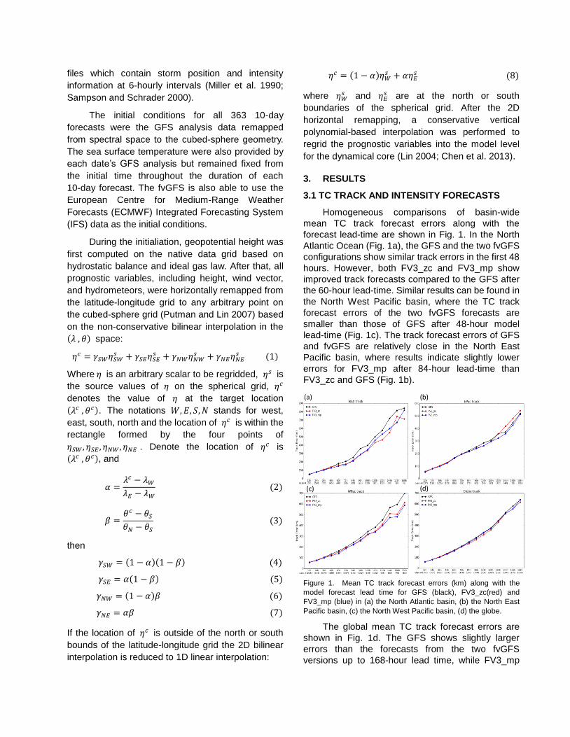
Homogeneous comparisons of basin-wide

mean TC track forecast errors along with the

forecast lead-time are shown in Fig. 1. In the North

Atlantic Ocean (Fig. 1a), the GFS and the two fvGFS

configurations show similar track errors in the first 48

hours. However, both FV3_zc and FV3_mp show

improved track forecasts compared to the GFS after

the 60-hour lead-time. Similar results can be found in

the North West Pacific basin, where the TC track

forecast errors of the two fvGFS forecasts are

smaller than those of GFS after 48-hour model

lead-time (Fig. 1c). The track forecast errors of GFS

and fvGFS are relatively close in the North East

Pacific basin, where results indicate slightly lower

errors for FV3_mp after 84-hour lead-time than

FV3_zc and GFS (Fig. 1b).

Figure 1. Mean TC track forecast errors (km) along with the

model forecast lead time for GFS (black), FV3_zc(red) and

FV3_mp (blue) in (a) the North Atlantic basin, (b) the North East

Pacific basin, (c) the North West Pacific basin, (d) the globe.

The global mean TC track forecast errors are

shown in Fig. 1d. The GFS shows slightly larger

errors than the forecasts from the two fvGFS

versions up to 168-hour lead time, while FV3_mp

(a) (b)

(d) (c)

shows slightly larger TC track forecast errors than

FV3_zc for most lead times after 84h.

To investigate the performance of TC intensity

forecasts, the wind-pressure relationships of TCs in

GFS and FV3_zc are compared to the best track

data in Fig. 2. For intense cyclones with observed

intensities exceeding 40 ms-1

, there is clearly a much

better relationship between sea level pressure (SLP)

and maximum 10-m wind speed for FV3_zc than for

the GFS. The model configuration of FV3_zc uses a

physics package nearly identical to that used in the

GFS, while the horizontal resolutions of the two

forecasts are also very close. Therefore, we believe

that the differences shown in Fig. 2 are primarily

from the replacement of the dynamical core. It is a

very encouraging result that an advanced dynamical

core is contributing to improving pressure-wind

relationship for TCs in a global model.

Figure 2. The relationship of maximum 10-m wind (ms-1) and

minimum sea level pressure (hPa) for TCs in (a) the North Atlantic

Ocean, (b) the North East Pacific basin, (c) the North Central

Pacific basin and (d) the North West Pacific basin. Forecast data

are plotted from every 6-hour lead time. The observations from

ATCF best-track data are denoted in black dots. Forecasts of GFS

cyclones are in blue dots and of FV3_zc are in red.

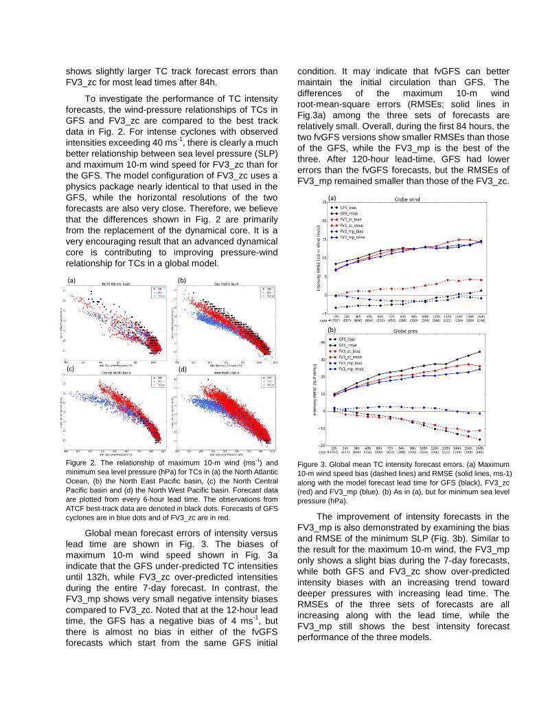
Global mean forecast errors of intensity versus

lead time are shown in Fig. 3. The biases of

maximum 10-m wind speed shown in Fig. 3a

indicate that the GFS under-predicted TC intensities

until 132h, while FV3_zc over-predicted intensities

during the entire 7-day forecast. In contrast, the

FV3_mp shows very small negative intensity biases

compared to FV3_zc. Noted that at the 12-hour lead

time, the GFS has a negative bias of 4 ms-1

, but

there is almost no bias in either of the fvGFS

forecasts which start from the same GFS initial

condition. It may indicate that fvGFS can better

maintain the initial circulation than GFS. The

differences of the maximum 10-m wind

root-mean-square errors (RMSEs; solid lines in

Fig.3a) among the three sets of forecasts are

relatively small. Overall, during the first 84 hours, the

two fvGFS versions show smaller RMSEs than those

of the GFS, while the FV3_mp is the best of the

three. After 120-hour lead-time, GFS had lower

errors than the fvGFS forecasts, but the RMSEs of

FV3_mp remained smaller than those of the FV3_zc.

Figure 3. Global mean TC intensity forecast errors. (a) Maximum

10-m wind speed bias (dashed lines) and RMSE (solid lines, ms-1)

along with the model forecast lead time for GFS (black), FV3_zc

(red) and FV3_mp (blue). (b) As in (a), but for minimum sea level

pressure (hPa).

The improvement of intensity forecasts in the

FV3_mp is also demonstrated by examining the bias

and RMSE of the minimum SLP (Fig. 3b). Similar to

the result for the maximum 10-m wind, the FV3_mp

only shows a slight bias during the 7-day forecasts,

while both GFS and FV3_zc show over-predicted

intensity biases with an increasing trend toward

deeper pressures with increasing lead time. The

RMSEs of the three sets of forecasts are all

increasing along with the lead time, while the

FV3_mp still shows the best intensity forecast

performance of the three models.

(a)

(d)

(b)

(c)

(a)

(b)

3.2 TESTS USING DIFFERENT INITIAL

CONDITIONS

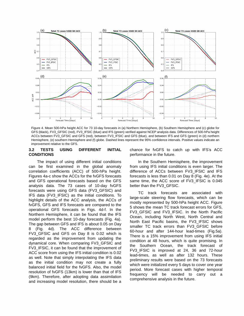
The impact of using different initial conditions

can be first examined in the global anomaly

correlation coefficients (ACC) of 500-hPa height.

Figures 4a-c show the ACCs for the fvGFS forecasts

and GFS operational forecasts based on the GFS

analysis data. The 73 cases of 10-day fvGFS

forecasts were using GFS data (FV3_GFSIC) and

IFS data (FV3_IFSIC) as the initial conditions. To

highlight details of the ACC analysis, the ACCs of

fvGFS, GFS and IFS forecasts are compared to the

operational GFS forecasts in Figs. 4d-f. In the

Northern Hemisphere, it can be found that the IFS

model perform the best 10-day forecasts (Fig. 4a).

The gap between GFS and IFS is about 0.05 on Day

8 (Fig. 4d). The ACC difference between

FV3_GFSIC and GFS on Day 8 is 0.02 which is

regarded as the improvement from updating the

dynamical core. When comparing FV3_GFSIC and

FV3_IFSIC, it can be found that the improvement of

ACC score from using the IFS initial condition is 0.02

as well. Note that simply interpolating the IFS data

as the initial condition may not create a fully

balanced initial field for the fvGFS. Also, the model

resolution of fvGFS (13km) is lower than that of IFS

(9km). Therefore, after adopting data assimilation

and increasing model resolution, there should be a

chance for fvGFS to catch up with IFS’s ACC

performance in the future.

In the Southern Hemisphere, the improvement

from using IFS initial conditions is even larger. The

difference of ACCs between FV3_IFSIC and IFS

forecasts is less than 0.01 on Day 8 (Fig. 4e). At the

same time, the ACC score of FV3_IFSIC is 0.045

better than the FV3_GFSIC.

TC track forecasts are associated with

large-scale steering flow forecasts, which can be

mostly represented by 500-hPa height ACC. Figure

5 shows the mean TC track forecast errors for GFS,

FV3_GFSIC and FV3_IFSIC. In the North Pacific

Ocean, including North West, North Central and

North East Pacific basins, the FV3_IFSIC shows

smaller TC track errors than FV3_GFSIC before

60-hour and after 144-hour lead-times (Fig.5a).

There is a 15% improvement from using IFS initial

condition at 48 hours, which is quite promising. In

the Southern Ocean, the track forecast of

FV3_IFSIC is improved at 24, 36 and 72-hour

lead-times, as well as after 132 hours. These

preliminary results were based on the 73 forecasts

which were initialized every 5 days to cover one year

period. More forecast cases with higher temporal

frequency will be needed to carry out a

comprehensive analysis in the future.

Figure 4. Mean 500-hPa height ACC for 73 10-day forecasts in (a) Northern Hemisphere, (b) Southern Hemisphere and (c) globe for

GFS (black), FV3_GFSIC (red), FV3_IFSIC (blue) and IFS (green) verified against NCEP analysis data. Differences of 500-hPa height

ACCs between FV3_GFSIC and GFS (red), between FV3_IFSIC and GFS (blue), and between IFS and GFS (green) in (d) northern

Hemisphere, (e) southern Hemisphere and (f) globe. Dashed lines represent the 95% confidence intervals. Positive values indicate an

improvement relative to the GFS.

(a) (b) (c)

(d) (e) (f)

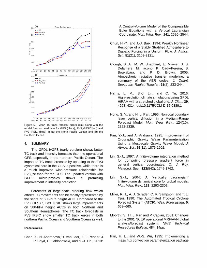
Figure 5. Mean TC track forecast errors (km) along with the

model forecast lead time for GFS (black), FV3_GFSIC(red) and

FV3_IFSIC (blue) in (a) the North Pacific Ocean and (b) the

Southern Ocean.

4. SUMMARY

The GFDL fvGFS (early version) shows better

TC track and intensity forecasts than the operational

GFS, especially in the northern Pacific Ocean. The

impact to TC track forecasts by updating to the FV3

dynamical core in the GFS is positive, while there is

a much improved wind-pressure relationship for

FV3_zc than for the GFS. The updated version with

GFDL micro-physics shows a promising

improvement in intensity prediction.

Forecasts of large-scale steering flow which

affects TC movements can be mostly represented by

the score of 500-hPa height ACC. Compared to the

FV3_GFSIC, FV3_IFSIC shows large improvements

on 500-hPa height ACCs in both Northern and

Southern Hemispheres. The TC track forecasts in

FV3_IFSIC show smaller TC track errors in both

northern Pacific Ocean and Southern Ocean as well.

References

Chen, X., N. Andronova, B. Van Leer, J. E. Penner, J.

P. Boyd, C. Jablonowski, and S.-J. Lin., 2013:

A Control-Volume Model of the Compressible

Euler Equations with a Vertical Lagrangian

Coordinate. Mon. Wea. Rev., 141, 2526–2544.

Chun, H.-Y., and J.-J. Baik, 1994: Weakly Nonlinear

Response of a Stably Stratified Atmosphere to

Diabatic Forcing in a Uniform Flow, J. Atmos.

Sci., 51(21), 3109-3121.

Clough, S. A., M. W. Shephard, E. Mlawer, J. S.

Delamere, M. Iacono, K. Cady-Pereira, S.

Boukabara, and P. D. Brown, 2005:

Atmospheric radiative transfer modeling: a

summary of the AER codes, J. Quant.

Spectrosc. Radiat. Transfer, 91(2), 233-244.

Harris, L. M., S.-J. Lin, and C. Tu, 2016:

High-resolution climate simulations using GFDL

HiRAM with a stretched global grid. J. Clim., 29,

4293–4314, doi:10.1175/JCLI-D-15-0389.1

Hong, S. Y., and H. L. Pan, 1996: Nonlocal boundary

layer vertical diffusion in a Medium-Range

Forecast Model, Mon. Wea. Rev., 124(10),

2322-2339.

Kim, Y.-J., and A. Arakawa, 1995: Improvement of

Orographic Gravity Wave Parameterization

Using a Mesoscale Gravity Wave Model, J.

Atmos. Sci., 52(11), 1875-1902.

Lin, S.-J., 1997: A finite-volume integration method

for computing pressure gradient force in

general vertical coordinates, Q. J. Roy.

Meteorol. Soc., 123(542), 1749-1762.

Lin, S.-J., 2004: A “vertically Lagrangian”

finite-volume dynamical core for global models,

Mon. Wea. Rev., 132, 2293-2307.

Miller, R. J., A. J. Scrader, C. R. Sampson, and T. L.

Tsui, 1990: The Automated Tropical Cyclone

Forecast System (ATCF). Wea. Forecasting, 5,

653–660.

Moorthi, S., H. L. Pan and P. Caplan, 2001: Changes

to the 2001 NCEP operational MRF/AVN global

analysis/forecast system, NWS Technical

Procedures Bulletin, 484, 14pp.

Pan, H. L., and W.-S. Wu, 1995: Implementing a

mass flux convection parameterization package

(a)

(b)

for the nmc medium-range forecast model,

NMC Office Note, No. 409, page 40pp.

Putman, W. M., and S.-J. Lin, 2007: Finite-volume

transport on various cubed-sphere grids. J.

Comput. Phys., 227, 55-78.

Sampson, C. R., and A. J. Schrader, 2000: The

Automated Tropical Cyclone Forecasting

System (version 3.2). Bull. Amer. Meteor. Soc.,

81, 1231–1240.