Tropical-cyclone flow asymmetries induced by a …roger/Publications/TCRR...Tropical-cyclone flow asymmetries induced by a uniform flow revisited ... b Dept. of Meteorology,

TROPICAL CYCLONE RESEARCH REPORTTCRR 1: 1–18 (2012)Meteorological InstituteLudwig Maximilians University of Munich

Tropical-cyclone flow asymmetries induced by a uniform flowrevisited

Gerald Thomsena, Roger K. Smitha, Michael T. Montgomeryb1

a Meteorological Institute, University of Munich, Munichb Dept. of Meteorology, Naval Postgraduate School, Monterey, CA

Abstract:We investigate the hypothesized effects of a uniform flow on the structural evolution of a tropical cyclone using an idealized, three-dimensional, convection-permitting, numerical model. The study addresses three outstanding basic questions concerning the effects ofmoist convection on the azimuthal flow asymmetries and provides a bridge between the problem of tropical cyclone intensification ina uniform flow and that in vertical shear.At any instant of time, explicit deep convection in the modelgenerates flow asymmetries that tend to mask the induced flowasymmetries predicted by a dry, slab boundary-layer model of Shapiro, whose results are frequently invoked as a benchmark forcharacterizing the boundary-layer induced vertical motion for a translating storm.In sets of ensemble experiments in which the initial low-level moisture field is randomly perturbed, time-averaged ensemble meanfields in the mature stage show a coherent asymmetry in the vertical motion rising into the eyewall. The maximum ascent occursabout 45 degrees to the left of the vortex motion vector, broadly in support of Shapiro’s results, in which it occurs aheadof the storm,and consistent with one earlier numerical calculation by Frank and Ritchie. Moreover, for the mainly strong vortices studied here(maximum wind speeds≈ 80 m s−1), this asymmetry is found only for background wind speeds larger than about 7 m s−1. There isconsiderable temporal variability in the structure of the low-level flow on a sub-hourly time scale as a result of transient convection,a finding that raises questions concerning the ability to be able to reliably determine vortex-scale flow asymmetries (especially in theradial direction) from dropwindsonde observations spreadover several hours.

KEY WORDS Hurricane; tropical cyclone; typhoon; boundary layer; vortex intensification

Date: April 7, 2014; Revised ; Accepted

1 Introduction

The predictability of tropical-cyclone intensification inathree-dimensional numerical model was investigated byNguyen et al.(2008): henceforth M1. They focussed ontwo prototype problems for intensification, which considerthe evolution of a prescribed, initially cloud-free, axisym-metric, baroclinic vortex over a warm ocean on anf -planeor beta-plane. A companion study of the same problemsusing a minimal three-dimensional model was carried outby Shin and Smith(2008). Both studies found that on anf -plane, the flow asymmetries that develop are highly sen-sitive to the initial low-level moisture distribution. Whena random moisture perturbation is added in the boundarylayer at the initial time, even with a magnitude that is belowthe accuracy with which moisture is normally measured,the pattern of evolution of the flow asymmetries is dra-matically altered and no two such calculations are alike indetail. The same is true also of calculations on aβ-plane,at least in the inner-core region of the vortex, within 100-200 km from the centre. Nevertheless the large-scaleβ-gyre

1Correspondence to: Michael T. Montgomery, Naval PostgraduateSchool, 159 Dyer Rd., Root Hall, Monterey, CA 93943. E-mail:[email protected]

asymmetries are similar in each realization and they remainwhen one calculates the ensemble mean. The implicationis that the inner-core asymmetries on thef - andβ-planeresult from the onset of deep convection in the model and,like deep convection in the atmosphere, they have a degreeof randomness, being highly sensitive to small-scale inho-mogeneities in the low-level moisture distribution. Suchinhomogeneities are a well-known characteristic of the realatmosphere (e.g.Weckwerth(2000)).

In the foregoing flow configurations, there was noambient flow and an important question remains: couldthe imposition of a uniform flow or a vertical shearflow lead to an organization of the inner-core convec-tion, thereby making its distribution more predictable?For example, there is evidence from observations (Kepert(2006a), Kepert (2006b), Schwendike and Kepert(2008))and from steady boundary layer models with varyingdegrees of sophistication that a translating vortex pro-duces a distinct asymmetric pattern of low-level con-vergence and vertical motion (Shapiro (1983), Kepert(2001), Kepert and Wang(2001)). There is much evi-dence also that vertical shear induces an asymmetry invortex structure (Raymond(1992), Jones(1995), Jones(2000), Smith et al. (2000), Frank and Ritchie (1999),Frank and Ritchie(2001), Reasor and Montgomery(2004),

Copyright c© 2012 Meteorological Institute

2 THOMSEN, G., R. K. SMITH, AND M. T. MONTGOMERY

Corbosiero and Molinari(2002), Corbosiero and Molinari(2003), Riemer et al. (2010)). An alternative questionwould be whether the flow asymmetries predicted by dry,steady boundary-layer models survive in the presence oftransient deep convection? The answer is not obvious to ussince such models tacitly assume that the convection is ableto accept whatever pattern and strength of upward verticalmotion the boundary layer determines at its top.

The important observational study byCorbosiero and Molinari(2003) showed that the dis-tribution of strong convection is more strongly correlatedwith vertical shear than with the storm translation vec-tor. Nevertheless, the question remains as to whetherstorm translation is important in organizing convectionin the weak shear case. Although the main purpose ofFrank and Ritchie(2001) was to investigate the effects ofvertical shear in a moist model with explicit representationof deep moist convection, they did carry out one simulationfor a weak uniform flow of 3.5 m s−1. In this they foundthat “ ... the upward vertical motion pattern varies betweenperiods that are almost axisymmetric and other periodswhen they show more of a azimuthal wavenumber-oneasymmetry, with maximum upward motion either aheador to the left of the track.” and “the frictional convergencepattern in the boundary layer causes a preference forconvective cells to occur generally ahead of the stormrelative to behind it, but this forcing is not strong enoughto maintain a constant asymmetric pattern”. Although theyshow only four time snapshots of the cloud water andrain water fields, the findings are at first sight contraryto the predictions of a steady boundary layer forced byan imposed gradient wind field above the boundary layeras in the other uniform flow studies cited above, but theorientation of the asymmetry is closest to the patternof vertical motion predicted byShapiro (1983). Evenso, snapshots are insufficient to show whether there isa persistent asymmetric pattern of deep convection in asuitable time average of the evolving flow.

There is disparity in the literature on the orientation offlow asymmetries that arise in the boundary layer, even inthe relatively simple configuration with no moist processes.For example, using quasi-linear and fully nonlinear, slabboundary layer models with constant depth,Shapiro(1983)showed that the strongest convergence (and hence verticalvelocity in the slab model) occurs on the forward side ofthe vortex in the direction of motion (see his Figures 5dand 6c). In contrast, the purely linear theory of Kepert(2001, left panel of his Figure 5) predicts that the strongestconvergence lies at 45 degrees to the right of the motionand the nonlinear calculations of Kepert and Wang (2001,bottom left panel of their Figure 10) predicts it to be at 90degrees to the right of motion. As noted by the respectiveauthors, a limitation of the foregoing studies is the fact thatthe horizontal flow above the boundary layer is prescribedand not determined as part of a full solution. Moreover, asnoted above, there is no guarantee that the ascent predicted

by the boundary layer solution can be “ventilated” by theconvection.

The presence of deep convection greatly compli-cates the situation and, as pointed out in M1 and byShin and Smith(2008), the random nature of the inner-coreflow asymmetries that convection leads to calls for a newmethodology to assess differences between two particularflow configurations. The reason is that the results of a sin-gle deterministic calculation in each configuration may beunrepresentative of a model ensemble in that configuration.Thus one needs to compare the ensemble means of suitablyperturbed ensembles of the two configurations, and/or tocarry out suitable time averaging. We apply this methodol-ogy here to extend the calculations of M1 to the prototypeproblem for a moving vortex, which considers the evolu-tion of an initially dry, axisymmetric vortex embedded in auniform zonal flow on a Northern Hemispheref -plane.

The scientific issues raised above motivate three spe-cific questions about the convective organization of a trans-lating vortex:

1 Does the imposition of a uniform flow in aconvection-permitting simulation lead to anorgani-zation of the inner-core convection to produce persis-tent azimuthal asymmetries in convergence and ver-tical motion?

2 If so, how do these asymmetries compare with thosepredicted by earliertheoretical studies where the hor-izontal flow above the boundary layer is prescribedand moist processes are not considered?

3 How do the asymmetries in low-level flow structureassociated with the storm translation compare withthose documented in recentobservational studies?

This paper seeks to answer these questions.The paper is structured as follows. We give a brief

description of the model in section2 and present the resultsof the main calculations for vortex evolution on anf -plane in section3. In section4 we describe the ensembleexperiments, where, as in M1, the ensembles are generatedby adding small moisture perturbations at low levels. Weexamine the asymmetric structure of boundary layer windsin section 5 and describe briefly a calculation using adifferent boundary-layer scheme section6. The conclusionsare given in section7.

2 The model configuration

The numerical experiments are similar to those described inM1 and are carried out also using a modified version of thePennsylvania State University-National Center for Atmos-pheric Research fifth-generation Mesoscale Model (MM5;version 3.6,Dudhia(1993); Grell et al.(1995)). The modelis configured with three domains with sides orientated east-west and north-south (Figure1). The outer and innermostdomains are square, the former 9000 km in size and the lat-ter 1500 km. The innermost domain is moved from east

Copyright c© 2012 Meteorological Institute TCRR 1: 1–18 (2012)

EYEWALL REPLACEMENT CYCLES 3

(a)

Figure 1. Configuration of the three model domains. The innerdomain is moved from east to west (the negativex-direction) atselected times to keep the vortex core away from the domain bound-

ary.

to west at selected times within an intermediate domainwith a fixed meridional dimension of 3435 km and a zonaldimension of up to 8850 km, depending on the backgroundwind speed. The first displacement takes place 735 min-utes after the initial time and at multiples of 1440 minutes(one day) thereafter. The frequency of the displacement isdoubled for a background wind speed of 12.5 m s−1. Thedistance displaced depends on the background wind speedin the individual experiments. The outer domain has a rel-atively coarse, 45-km, horizontal grid spacing, reducing to15 km in the intermediate domain and 5 km in the inner-most domain. The two inner domains are two-way nested.In all calculations there are 24σ-levels in the vertical, 7of which are below 850 mb. The model top is at a pres-sure level of 50 mb. The calculations are performed on anf -plane centred at 20◦N.

To keep the experiments as simple as possible, wechoose the simplest explicit moisture scheme, one thatmimics pseudo-adiabatic ascent1. In addition, for all but

1If the specific humidity,q, of a grid box is predicted to exceed thesaturation specific humidity,qs(p, T ) at the predicted temperatureT andpressurep, an amount of latent heatL(q − qs) is converted to sensibleheat raising the temperature bydT = L(q − qs)/cp andq is set equal toqs, so that an amount of condensatedq = q − qs is produced. (HereLis the coefficient of latent heat per unit mass andcp is the specific heatof dry air at constant pressure.) The increase in air parcel temperatureincreasesqs, so that a little less latent heat than the first estimate needsto be released and a little less water has to be condensed. Thepreciseamount of condensation can be obtained by a simple iterativeprocedure.Convergence is so rapid that typically no more than four iterations arerequired.

one experiment we choose the bulk-aerodynamic param-eterization scheme for the boundary layer. One addi-tional calculation is carried out using the Gayno-Seamanboundary-layer scheme (Shafran et al.(2000)) to investi-gate the sensitivity of the results to the scheme used.

The surface drag and heat and moisture exchange coef-ficients are modified to incorporate the results of the cou-pled boundary layer air-sea transfer experiment (CBLAST;seeBlack et al.(2007), andZhang et al.(2009)). The sur-face exchange coefficients for sensible heat and moistureare set to the same constant,1.2× 10−3, and that formomentum, the drag coefficient, is set to0.7× 10−3 +1.4× 10−3(1− exp(−0.055|u|)), where |u| is the windspeed at the lowest model level. The fluxes between theindividual model layers within the boundary layer are thencalculated using a simple downgradient diffusive closure inwhich the eddy diffusivity depends on strain rate and staticstability (Grell et al.(1995), Smith and Thomsen (2010)).

The exchange coefficient for moisture is set to zeroin the two outer domains to suppress the build up thereof ambient Convective Available Potential Energy (CAPE).Because of the dependence of the moisture flux on windspeed, such a build up would be different in the experimentswith different wind speeds. The sea surface temperatureis set to a constant 27oC except in one experiment whereit was set to 25oC to give a weaker mature vortex. Theradiative cooling is implemented by a Newtonian coolingterm that relaxes the temperature towards that of the initialprofile on a time scale of 1 day. This initial profile isdefined in pressure coordinates rather than the model’sσ-coordinates so as not to induce a thermal circulationbetween southern and northern side of the model domain.

In each experiment, the initial vortex is axisymmetricwith a maximum tangential wind speed of 15 m s−1

at the surface at a radius of 120 km. The strength ofthe tangential wind decreases sinusoidally with height,vanishing at the top model level (50 mb). The vortex isinitialized to be in thermal wind balance with the wind fieldusing the method described bySmith(2006). The far-fieldtemperature and humidity are based on Jordan’s Caribbeansounding (Jordan(1958)). The vortex centre is defined asthe centroid of relative vorticity at 900 mb over a circularregion of 200 km radius from a “first-guess” centre, whichis determined by the minimum of the total wind speed at900 mb, and the translation speed introduced later is basedon the movement of this centre.

2.1 The control experiments

Six control experiments are discussed, five with a uniformbackground easterly wind field,U , and the other withzero background wind. Values ofU are 2.5 m s−1, 5 ms−1, 7.5 m s−1, 10 m s−1 and 12.5 m s−1, adequatelyspanning the most common range of observed tropical-cyclone translation speeds. All these experiments employthe bulk aerodynamic option for representing the boundarylayer and have a sea surface temperature (SST) of 27oC.



Figure 2. Time series of maximum total wind speed at 850 mb,V Tmax, for the six experiments with different background windspeedsU in m s−1 as indicated, and for the experiment withU = 5.0

m s−1, but with the sea surface temperature reduced to 25oC. Thetime series have been smoothed with a five-point filter to highlight

the differences between them.

Two additional experiments haveU = 5 m s−1, one withan SST of 25oC, and the other with the Gayno-Seamanboundary-layer scheme.

2.2 Ensemble experiments

As in M1, sets of ensemble calculations are carried out forthe control experiments. These are similar to the main cal-culations, but have a random perturbation with a magnitudebetween±0.5 g kg−1 added to the water-vapour mixingratio at each grid point up to 950 mb at the initial time.In order to keep the mass field unchanged, the tempera-ture is adjusted at each point to keep the virtual temperatureunchanged. A five-member ensemble is constructed for allvalues ofU exceptU = 5 m s−1, for which a ten2 memberensemble is constructed.

3 Results of five deterministic calculations

3.1 Vortex evolution and motion

Figure 2 shows time-series of the maximum total windspeed,V Tmax at 850 mb (approximately 1.5 km high)during a 7 day (168 hour) integration in the six controlexperiments and in that withU = 5 m s−1 and an SST of25oC. The last experiment will be discussed in section3.3.As in many previous experiments, the evolution begins witha gestation period during which the vortex slowly decays

2The ten member ensemble was the first to be constructed. Examinationof the wind speed maxima for this ensemble suggested that computation-ally less expensive five member ensembles would suffice to span the rangeof variability. On this basis, five-member ensemble plus themain deter-ministic experiment was used for the other background flow speeds.

due to surface friction, but moistens in the boundary layerdue to evaporation from the underlying sea surface. Thisperiod lasts approximately 9 hours during which time themaximum total wind speed decreases by about 2.0 m s−1.

The imposition of friction from the initial instant leadsto inflow in the boundary layer and outflow above it, theoutflow accounting for the initial decrease in tangentialwind speed through the conservation of absolute angu-lar momentum. The inflow is moist and as it rises out ofthe boundary layer and cools, condensation progressivelyoccurs in some grid columns interior to the correspond-ing radius of maximum tangential wind speed. In thesecolumns, existing relative vorticity is stretched and ampli-fied leading to the formation of localized deep vorticalupdraughts. Collectively, these updraughts lead to the con-vergence of absolute angular momentum above the bound-ary layer and thereby to the spin up of the bulk vortex(see e.g.Bui et al.(2009)). Then, as the bulk vortex intensi-fies, the most intense tangential wind speeds develop in theboundary layer (Smith et al.(2009)).

As the updraughts develop, there ensues a periodlasting about 5 days during which the vortex progressivelyintensifies. During this time,V Tmax increases from itsminimum value of between 12.5 and 25 m s−1 to a finalvalue of up to 90 m s−1 at the end of the experiment.The vortex in the quiescent environment is the first toattain an approximate quasi-steady state after about 6 days,but all except possibly that forU = 10 m s−1 appear tohave reached such a state by 7 days. For all values ofU ,there are large fluctuations inV Tmax (up to ±5 m s−1

before time-smoothing) during the period of intensification.Indeed, except in the experiment with an SST of 25oC, thefluctuations in an individual experiment during this periodare comparable with the maximum deviations between thedifferent experiments to the extent that it is pertinent to askif the differences between these experiments are significant.We examine this question in section4.

The translation speed (calculated as detailed in section2) tends to be fractionally smaller than the backgroundwind speed, especially in the mature stage when it isbetween 20% and 25% less. The translation speeds forU =7.5 m/s, 10 m/s and 12.5 m/s are about 5.9, 7.5 and 9.5 m/s,respectively. The reason for the lower translation speed ispresumably because the tangential circulation of the vortexis strongest at low levels where the background wind is,itself, reduced in strength by surface friction.

3.2 Structure changes

The evolution in vortex structure during the intensificationstage is exemplified by the contours of vertical velocity at850 mb at selected times for the control experiment withU = 5 m s−1. These contours are shown in Figures3 and4. At early times, convective cells begin to develop in theforward left (i.e. southwest) quadrant (Figure3a), where,as shown below, the boundary-layer-induced convergenceis large. However, cells subsequently develop clockwise



(a) (b)

(c) (d)

(e) (f)

Figure 3. Contours of vertical velocity at 850 mb at times indicated in the top right of each panel during the vortex evolution. (a)-(d) for theexperiment withU = 5.0 m s−1 (from right to left), and (e) and (f) for the experiment with the zero background flow. Contour interval: thickcontours 0.5 m s−1, thin contours 0.1 m s−1. Positive velocities (solid/red lines), negative velocities (dashed/blue lines). The zero contour is

not plotted. The arrow indicates the direction of vortex motion.Copyright c© 2012 Meteorological Institute TCRR 1: 1–18 (2012)


(a) (b)

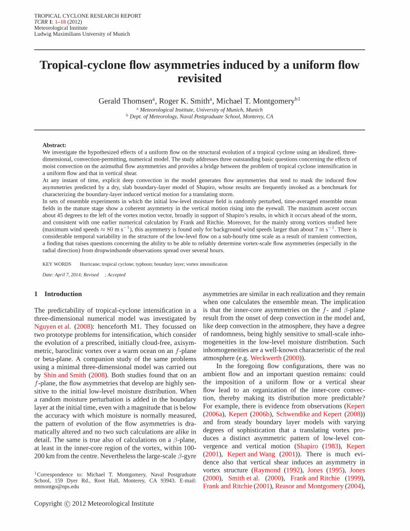
Figure 4. Contours of vertical velocity at 850 mb at (a) 60 hours, and (b) 96 hours, during the vortex evolution for the experiment withU = 5.0 m s−1 (from right to left). Contour interval: thick contours 0.5 ms−1, thin contours 0.1 m s−1. Positive velocities (solid/red lines),

negative velocities (dashed/blue lines). The zero contouris not plotted. The arrow indicates the direction of vortex motion.

(a) (b)

Figure 5. Contours of divergence at 500 m at for the experiment with U = 5.0 m s−1: (a) between 3-5 hours (contour interval1× 10−5 s−1.

Positive contours (solid/red) and negative values (dashed/blue).) and (b) between6 3

4− 7 days (contour interval: thick contours5× 10

−4

s−1, thin contours5× 10−5 s−1. Positive contours (solid/red), negative values (dashed/blue)), zero contour thin, solid and black. The arrow

indicates the direction of vortex motion. Note that the domain shown is only half the size of that in Figures3 and4.

(upstream in the tangential circulation) in the space of twohours to the forward quadrant (Figure3b) and over the nexttwo hours to the forward right and rear right quadrants(Figure 3c). The increased surface moisture fluxes (notshown)on the right side of the storm, where the earth-relative wind speeds are stronger, may play a role insupporting convection also. It should be emphasized that,as in the calculations in M1, the convective cells are deep,extending into the upper troposphere (not shown here).

By 24 hours, convective cells are distributed over allfour quadrants with little obvious preference for a particularsector. Moreover, they amplify the vertical component of

local low-level relative vorticity by one or two orders ofmagnitude (not shown). For comparison, panels (e) and (f)of Figure3 show the early evolution of cells in the maincalculation with zero background flow, which, as expected,shows no preference for cells to develop in a particularsector.

As time proceeds, the convection becomes more orga-nized (Figure4), showing distinctive banded structures, buteven at 90 h, its distribution is far from axisymmetric, evenin the region within 100 km of the axis. However, as shownlater, the vortex does develop an annular ring of convectionwith an eye-like feature towards the end of the integration.



(a) (b)

Figure 6. Contours of divergence at 500 m at for the experiment with U = 5.0 m s−1 and a sea surface temperature of 25oC: (a) between 3-5hours (contour interval1× 10

−5 s−1). (b) between6 3

4− 7 days (contour interval: thick contours5× 10

−4 s−1, thin contours5× 10−5

s−1. Positive contours (solid/red), negative values (dashed/blue), zero contour thin, solid and black. The arrow indicates the direction of vortexmotion. Note that the domain shown is only half the size of that in Figure4.

Figure5 shows the pattern of convergence at a heightof 500 m averaged between 3 and 5 h and6 3

4− 7 days3

in the case withU = 5 m s−1. This height is typically thatof the maximum tangential wind speed and about half thatof the ‘mean’ inflow layer in the mature stage (see section5). The period 3-5 hours is characteristic of the gestationperiod during which the boundary layer is moistening, butbefore convection has commenced. During this period, theconvergence is largest on the forward side of the vortex,explaining why the convective instability is first releasedon this side. There is a region of divergence in the rear leftsector. The pattern is similar to that predicted by Shapiro(19834), but in Shapiro’s calculation, which, at this stagewas for a stronger symmetric vortex with a maximumtangential wind speed of 40 m s−1 translating at a speedof 10 m s−1, the divergence region extends also to the rearright of the track.

In the mature stage in our calculation, the pattern ofconvergence is rather different from that in Shapiro’s cal-culation and is much more symmetric, presumably becauseat this stage the vortex is twice as strong as Shapiro’s andthe translation speed is only half. Notably, outside the ringof strong convergence that marks the eyewall, the vortexis almost surrounded by a region of low-level divergence,except for the narrow band of convergence wrapping into

3The six hour averaging period is chosen to span a reasonable numberof fluctuations in the azimuthally-averaged tangential wind field shownin Figure 2 before the curves are smoothed. However, the pattern ofconvergence is not appreciably different when a twelve hourperiod ischosen.4See his Figure 5d, but note that the vortex translation direction is orienteddifferently to that in our configuration.

the eyewall from the forward right to the forward left quad-rants. In the next section we examine the differences inbehaviour for a weaker vortex.

It is perhaps worth remarking that the ring of diver-gence inside the ring of strongest convergence in Figure5c is associated with the upflow from the boundary layer,which is being centrifuged outwards as part of the adjust-ment of this supergradient flow to a state of local gradientwind balance (Smith et al. (2009)). The area of conver-gence in the small central region of the vortex is presum-ably the weak Ekman-like pumping one would expect in arotating vortex with weak frictional inflow in the boundarylayer.

3.3 Calculations for a weaker vortex

To examine the questions raised in the previous sectionconcerning possible differences when the vortex is muchweaker, we repeated the experiment withU = 5 m s−1

with the sea surface temperature reduced by 2oC to 25oC.Figure2 shows the variation of total wind speed at 850 mbin this case. The maximum wind speed during the maturestage is considerably reduced, compared with that in theother experiments, with the average wind speed duringthe last 6 hours of the calculation being only about 40m s−1. However, as expected, the evolution in verticalvelocity at 850 mb is similar to that in Figure3. Figure6 shows the patterns of divergence at a height of 500 maveraged during 3-5 hours and during the last 6 hoursof this calculation. These should be compared with thecorresponding fields in Figure5. In the early period (panel(a)), the patterns are much the same, although the maximum



magnitudes of asymmetric divergence and convergenceare slightly larger when the sea surface temperature isreduced. A plausible explanation for this difference is thereduced Rossby elasticity in the weaker vortex (McIntyre(1993)). In the mature stage (panel (b)), the central ring ofdivergence marking the eye is much larger in the case of theweaker vortex and the region of convergence surroundingit that marks the eyewall is broader and more asymmetric.Like the stronger vortex and that in Shapiro’s calculation,the largest convergence remains on the forward side of thevortex with respect to its motion. Of course, the motion-induced asymmetry in the convergence field is much morepronounced in the case of the weaker vortex.

4 Ensemble experiments

As pointed out by M1 and Shin and Smith (2008), theprominence of deep convection during the vortex evolutionand the stochastic nature of convection, itself, means thatthe vortex asymmetries will have a stochastic componentalso. Thus, a particular asymmetric feature brought aboutby an asymmetry in the broadscale flow (in our casethe uniform flow coupled with surface friction) may beregarded as significant only if it survives in an ensembleof experiments in which the details of the convectionare different. For this reason, we carried out a seriesof ensemble experiments in which a random moistureperturbation is added to the initial condition in the controlexperiments as described in section 2.2. We begin byinvestigating the effects of this stochastic component on thevortex intensification and go on to examine the effects onthe vortex structure in the presence of uniform flows withdifferent magnitudes.

4.1 Stochastic nature of vortex evolution

For simplicity, we examine first the time series of theensemble-mean of the maximum total wind speed,V Tmax,at 850 mb for two of the control experiments, those withbackground flows of 5 m s−1 and 10 m s−1. These areshown in Figure7a, together with the maximum and mini-mum values ofV Tmax at each time. The latter indicate therange of variability for each set of ensembles. There are twofeatures of special interest:

• Although the ensemble mean intensity of the run withU = 5 m s−1 is lower than that withU = 10 m s−1

at early times, with little overlap of the ensemblespread, the mean withU = 5 m s−1 exceeds that ofU = 10 m s−1 after about 108 hours, even thoughthere remains a region of overlap in the ensemblespread to 168 hours.

• There is a significant difference between the maxi-mum and minimum intensity in a particular run atany one time, being as high as 20 m s−1 in the caseU = 10 m s−1 at about 6 days.

The foregoing comparison provides a framework forre-examining the differences in intensity between the con-trol experiments with different values of background flowshown in Figure2. The comparison affirms the need toexamine ensemble-mean time series rather than those ofsingle deterministic runs. A comparison correspondingwith the deterministic runs of Figure2 is made in Figure7b, which shows time series of the ensemble mean for theexperiments withU = 0, 5, 7.5, 10 and 12.5 m s−1. It isclear from this figure that the intensification rate decreasesbroadly with increasing background flow speed and thatthe mature vortex intensity decreases also, although thereis a period of time, between about 4 and 7 days when theensemble-mean intensity forU = 10 is less than that forU = 12.5 m s−1. Moreover, the differences between theintensity of the pairs of ensembles withU = 5 and7.5 ms−1 andU = 10 and12.5 m s−1 at 7 days are barely signifi-cant. Finally we note that comparison of plots of the eleven5

V Tmax-time series forU = 5 m s−1 with the six such timeseries for the other ensemble sets suggests that five ensem-bles together with the corresponding control experimentgive an acceptable span of the range of variability in inten-sity in each case (not shown).

The foregoing results are consistent with those ofZeng et al.(2011), who presented observational analysesof the environmental influences on storm intensity andintensification rate based on reanalysis and best track dataof Northwest Pacific storms. While they considered abroader range of latitudes, up to 50oN, and of stormtranslation speeds of up to 30 m s−1, the data that aremost relevant to this study pertain to translation speedsbetween 3 and 12 m s−1. The most intense tropical cyclonesand those with the most rapid intensification rates werefound to occur in this range when there is relatively weakvertical shear. Most significantly, their data have a largeamount of scatter in this range and do not show an obviousrelationship between intensity and translation speed.

An investigation of the precise reasons why a uniformflow reduces the rate of intensification and mature intensityas the background flow increases is beyond the scope of thisstudy.

4.2 Stochastic nature of vortex structure

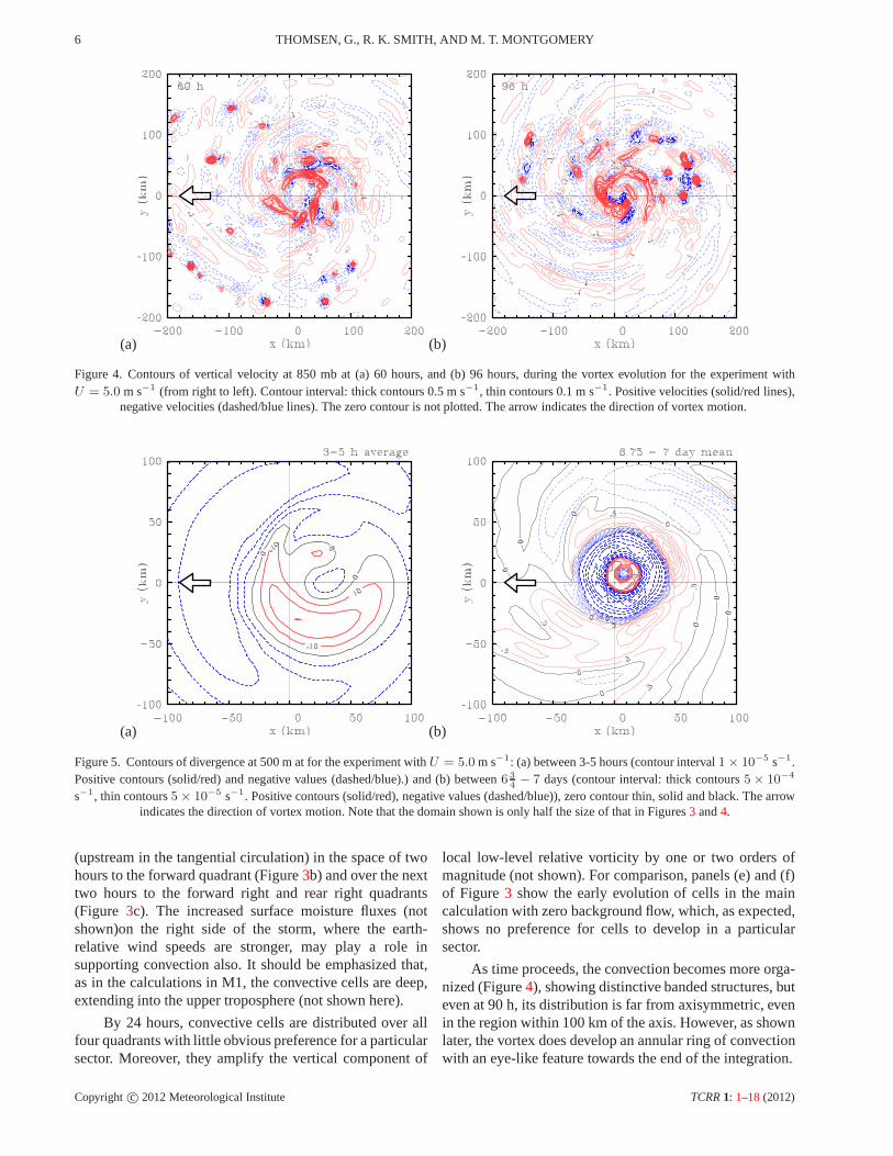
The first four panels of Figure8 show the time-averagedvertical velocity fields for the last 6 hours of integration(6 3

4- 7 days) in three of the experiments withU = 10.0

m s−1, including the control experiment and two ensem-ble experiments and in the six-member ensemble mean. Inall fields, including the ensemble mean, there is a promi-nent azimuthal wavenumber-1 asymmetry, with maximumupflow in the forward left quadrant and maximum subsi-dence in the eye to the left of the motion vector. Similarresults are obtained forU = 7.5 m s−1 and12.5 m s−1 (not

5We include the main calculation as part of the ensemble mean whenaveraging.



(a) (b)

Figure 7. (a) Time series of the ensemble-mean, maximum total wind speed,V Tmax, at 850 mb for the control experiments with a backgroundflow of 5 m s−1 (middle red curve) and 10 m s−1 (middle blue curves). The thin curves of the same colour showthe maximum and minimumvalues ofV Tmax for a particular run at a given time. (b) Time series of the ensemble-meanV Tmax for the experiments withU = 0, 5, 7.5,

10 and 12.5 m s−1.

shown). Inspection of the field forU = 5 m s−1 suggeststhat the most prominent asymmetry in the upward verticalvelocity is at azimuthal wavenumber-4 (Fig.8f), which isa feature also of the ensemble mean of calculations for aquiescent environment (Fig.8e). Since the case of a quies-cent environment would be expected to have no asymmetryfor a sufficiently large ensemble, we are inclined to con-clude that the wavenumber-4 asymmetry in the case withU = 5 m s−1 is largely a feature of the limited grid reso-lution (the 100 km square domain in Figure8 is spannedby only21× 21 grid points). Therefore we do not attributemuch significance to the wavenumber-4 component of theasymmetry in panels (e)-(f).

On the basis of these results, we are now in a positionto answer the first of the three questions posed in theIntroduction: does the imposition of a uniform flow in aconvection-permitting simulation lead to an organizationofthe inner-core convection so as to produce asymmetries inlow-level convergence and vertical motion? The answer tothis question is a qualified yes, the qualification being thatthe effect is barely detectable for the strong vortices thatarise in our calculations and for background flow speedsbelow about 7 m s−1. However, the effect increases withbackground flow speed and there is a more prominentazimuthal wavenumber-1 asymmetry in the calculation fora weaker storm withU = 5 m s−1 (see section3.3 andFigure6b).

We are in a position also to answer the second ofthe three questions: how do the asymmetries compare withthose predicted by earlier studies? For background flowspeeds of 7.5 m s−1 and above, the ensemble mean ver-tical velocity asymmetry, which has a maximum velocityin the forward left quadrant in our calculations, is closestto the predictions of Shapiro (1983). These predictions arebased on solutions of a truncated azimuthal spectral model

for the boundary layer of a translating vortex. In his non-linear solution, Shapiro found the maximum convergence(and hence vertical motion in his slab model) to be in thedirection of storm motion, while we find it to be approxi-mately 45o to the left thereof. Shapiro analyzed also linearand “quasi-linear” truncations. He noted that the solutionof the linear truncation is inaccurate in characterizing theasymmetries. In the quasi-linear truncation, the feedbackfrom wavenumbers-1 and -2 to wavenumbers-0 and -1 inthe nonlinear advective terms is neglected (i.e. backscatteris neglected). While there are some small quantitative dif-ferences between the quasi-linear and nonlinear solutions,the patterns of the flow asymmetries are similar (comparehis Figs. 5 and 6). Based on his analyses, Shapiro offers aclear articulation and quantification of the self-sharpeningeffect of azimuthal wave scattering on the translating meanvortex. We conclude that Shapiro’s nonlinear model pro-vides an acceptable zero-order description of the boundary-layer asymmetries that survive the transient effects of deepconvection. The reasons for the discrepancies between oursimulations and Shapiro’s results are presumably because,in our calculations, the vortex flow above the boundarylayer is determined as part of a full solution for the flowand is not prescribed. In other words, the wind and pres-sure fields at the top of the boundary layer adjust so that, inthe quasi-steady state, deep convection ventilates the massthat exits the boundary layer.

The asymmetry in vertical velocity in our model devi-ates significantly from that in Kepert’s (2001) linear theory,where the maximum vertical velocity is at 45o to therightof the motion vector (see his Figure 5 left)and even morefrom that in the nonlinear numerical calculation of Kepertand Wang (2001), where the maximum is at 90o to therightof the motion vector (see their Figure 10). The reasons forthe discrepancies between Shapiro’s results and those of



(a) (b)

(c) (d)

Figure 8. Contours of vertical velocity at 850 mb averaged during the period6 3

4− 7 days about the centre of minimum total wind speed at

this level. (a-d) The experiments withU = 10 m s−1; (a) The control experiment; (b) and (c) two ensemble experiments, and (d) the averageof the main and five ensemble experiments. For comparison, panels (e) and (f) show the ensemble mean fields for the experiments withU = 0

m s−1 andU = 5 m s−1, respectively. Contour interval 0.5 m s−1. Positive velocities (solid/red lines), negative velocities (dashed/blue lines),zero contour thin, solid and black. Filled contours indicate values larger in magnitude than 3 m s−1. The arrow indicates the direction of vortex

motion.

Kepert (2001) and Kepert and Wang (2001) are unclear:although the last two papers cited Shapiro’s earlier work,they did not comment on the differences between their find-ings and his.

4.3 Wind asymmetries

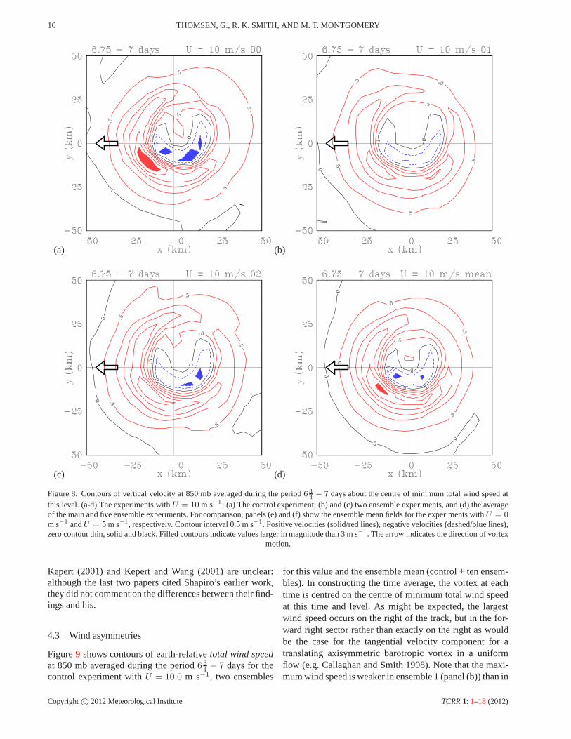
Figure9 shows contours of earth-relativetotal wind speedat 850 mb averaged during the period6 3

4− 7 days for the

control experiment withU = 10.0 m s−1, two ensembles

for this value and the ensemble mean (control + ten ensem-bles). In constructing the time average, the vortex at eachtime is centred on the centre of minimum total wind speedat this time and level. As might be expected, the largestwind speed occurs on the right of the track, but in the for-ward right sector rather than exactly on the right as wouldbe the case for the tangential velocity component for atranslating axisymmetric barotropic vortex in a uniformflow (e.g. Callaghan and Smith 1998). Note that the maxi-mum wind speed is weaker in ensemble 1 (panel (b)) than in



(a) (b)

(c) (d)

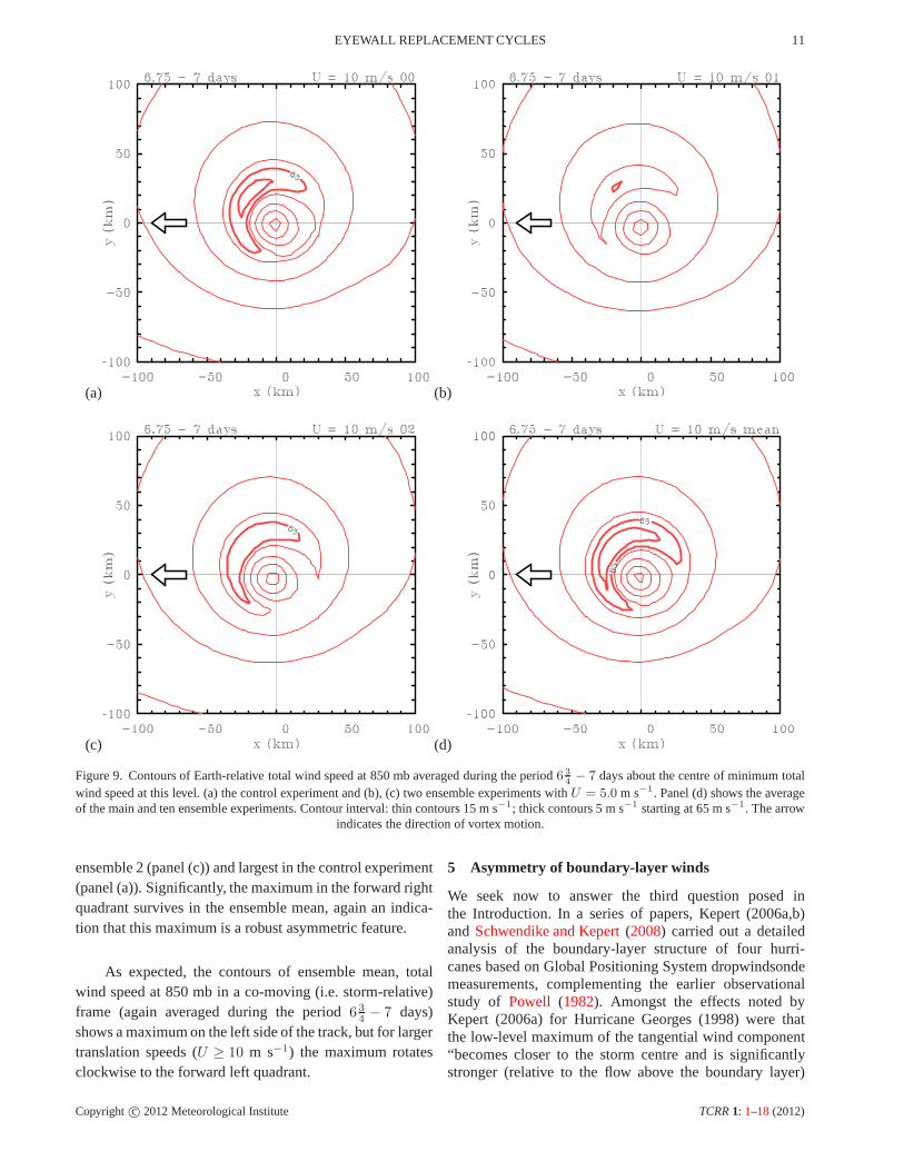
Figure 9. Contours of Earth-relative total wind speed at 850mb averaged during the period6 3

4− 7 days about the centre of minimum total

wind speed at this level. (a) the control experiment and (b),(c) two ensemble experiments withU = 5.0 m s−1. Panel (d) shows the averageof the main and ten ensemble experiments. Contour interval:thin contours 15 m s−1; thick contours 5 m s−1 starting at 65 m s−1. The arrow

indicates the direction of vortex motion.

ensemble 2 (panel (c)) and largest in the control experiment(panel (a)). Significantly, the maximum in the forward rightquadrant survives in the ensemble mean, again an indica-tion that this maximum is a robust asymmetric feature.

As expected, the contours of ensemble mean, totalwind speed at 850 mb in a co-moving (i.e. storm-relative)frame (again averaged during the period6 3

4− 7 days)

shows a maximum on the left side of the track, but for largertranslation speeds (U ≥ 10 m s−1) the maximum rotatesclockwise to the forward left quadrant.

5 Asymmetry of boundary-layer winds

We seek now to answer the third question posed inthe Introduction. In a series of papers, Kepert (2006a,b)and Schwendike and Kepert(2008) carried out a detailedanalysis of the boundary-layer structure of four hurri-canes based on Global Positioning System dropwindsondemeasurements, complementing the earlier observationalstudy of Powell (1982). Amongst the effects noted byKepert (2006a) for Hurricane Georges (1998) were thatthe low-level maximum of the tangential wind component“becomes closer to the storm centre and is significantlystronger (relative to the flow above the boundary layer)



(a) (b)

(c) (d)

Figure 10. Height-radius cross sections showing isotachs of the wind component in different compass directions (x) in the co-moving frame.The data are for the control calculation withU = 5 m s−1 and a sea surface temperature of 25oC, and are averaged over the last 6 hours ofthe calculation. (a) south to north, (b) southeast to northwest, (c) west to east, (d) southwest to northeast. Contour values: 5 m s−1. Positive

contours solid/red, negative contours dashed/blue. The zero contour is not plotted.

on the left of the storm than the right”. He noted alsothat “there is a tendency for the boundary-layer inflow tobecome deeper and stronger towards the front of the storm,together with the formation of an outflow layer above,which persists around the left and rear of the storm.” Weexamine now whether such features are apparent in thepresent calculations.

Figure 10 shows height-radius cross sections of thetangential and radial wind component in the co-movingframe in different compass directions for the main calcu-lation with U = 5 m s−1. Panels (a) and (b) of this figureshow time-averaged isotachs of the tangential winds in thelast six hours of the calculation in the west-east (W-E) andsouth-north (S-N) cross sections to a height of 3 km. Thesedo show a slight tendency for the maximum tangential windcomponent at a given radius to become lower with decreas-ing radius as the radius of the maximum tangential windis approached. Moreover, the maximum tangential windspeed occurs on the left (i.e. southern) side of the stormas found by Kepert. In fact, the highest wind speeds extendacross the sector from southwest to southeast and the lowestwinds in the sector northeast to northwest6.

Panels (c)-(f) of Figure10 show the correspondingtime-averaged isotachs of the radial winds in the west-east,

6The maximum tangential wind speeds in the various compass directionsare: W 77.1 m s−1, SW 85.9 m s−1, S 85.9 m s−1, SE 84.0 m s−1, E78.3 m s−1, NE 73.7 m s−1, N 71.0 m s−1, NW 73.9 m s−1

southwest-northeast (SW-NE), south-north and southeast-northwest (SE-NW) cross sections. Thus the strongest anddeepest inflow occurs in the sector from northwest tosouthwest (i.e. the sector centred on the direction of stormmotion) and the weakest and shallowest inflow in the sectorsoutheast to east7. These results are broadly consistent withthe Kepert’s findings. Note that, in contrast to Shapiro’sstudy, there is inflow in all sectors, presumably because ofthe much stronger vortex here.

The strongest outflow lies in the south to southeast sec-tor (panels (c) and (d) of Figure10), which is broadly con-sistent also with Kepert’s findings for Hurricane Georges.

While the azimuthally-averaged radial velocity com-ponent may appear to be somewhat large in some of thecross sections, we would argue that the values are notunreasonable. For example, Kepert (2006a, Figure 9) showsmean profiles with inflow velocities on the order of 30 ms−1 for Hurricane Georges (1998) with a mean near-surfacetangential wind speed of over 60 m s−1. Moreover, Kepert(2006b, Figure 6) shows maximum inflow velocities forHurricane Mitch (1998) on the order of 30 m s−1 with amean near-surface tangential wind speed on the order of50 m s−1. In our calculations the mean total near-surfacewind speed is on the order of 75 m s−1. The boundary

7The maximum radial wind speeds in the various compass directions are:W 43.5 m s−1, SW 39.3 m s−1, S 34.8 m s−1, SE 29.7 m s−1, E 29.1 ms−1, NE 33.1 m s−1, N 38.5 m s−1, NW 42.6 m s−1.



layer composite derived from dropsondes released fromresearch aircraft in Hurricane Isabel (2003) in the eyewallregion byMontgomery et al.(2006) shows a similar ratioof 0.5 between the maximum mean near-surface inflow tomaximum near-surface swirling velocity. The recent drop-sonde composite analysis of many Atlantic hurricanes byZhang et al.(2011b) confirms that a ratio of 0.5 for themean inflow to mean swirl for major hurricanes appears tobe typical near the surface.

Despite the good overall agreement with Kepert’sobservational study in the time-averaged fields, the fieldsat individual times show considerable variability betweenthe 15 minute output times. For example, panels (g) and (h)show the radial wind in the southeast to northwest sectorat 162.5 h and 162.75 h, which should be compared withthe corresponding time mean panel (d). At 162.5 h, theflow from the northwest is strong and crosses the vortexcentre, the maximum on this side being 54.0 m s−1 8. Incontrast, the maximum inflow on the southeastern side inthis cross section is 28.3 m s−1. Fifteen minutes later, themaximum inflow on the two sides of this cross section iscomparable, but slightly larger on the southeastern side,36.1 m s−1, compared with 33.5 m s−1 on the northwesternside. While some of this extreme temporal variability islikely a reflection of the calculated vortex centre togetherwith the possible aliasing described in footnote 8, thevariability in the centre position from a smooth track isto be expected because of the stochastic nature of deepconvection in the eyewall region and is not a flaw of theparticular centre-finding method employed. Indeed, thisissue is a challenge also in any observational study oftropical cyclone flow asymmetries asymmetries.

The variability of the flow structures discussed aboveis not represented in calculations that assume adry symmet-ric translating vortex moving at uniform speed such as thoseof Shapiroop. cit. and Kepert (2006a,b). However, the largevariability is supported by Kepert’s analysis of observa-tional data. For example, Kepert (2006a, p2178) states “Theradial flow measurements show neither systematic variationnor consistency from profile to profile, possibly becausethe measurements were sampling small-scale, vertically-coherent, but transient features”. Our calculations supportthis finding and suggest that the ‘transient features’ areassociated with deep convection.

At this time there does not appear to be a satisfac-tory theory to underpin the foregoing findings concern-ing the asymmetry in the depth of the inflow, which isan approximate measure for the boundary layer depth. Ofthe two theories that we are aware of, Shapiro’s (1983)study assumes a boundary layer of constant depth, but itdoes take into account an approximation to the nonlinear

8We caution that the large maximum in the radial velocity componentin panel (g) and the fact that the flow in this cross section is significantlynonzero at the identified centre suggests that, at least in part, there is somealiasing of the tangential component of flow into the radial component atthis time.

acceleration terms in the inner core of the vortex. In con-trast, Kepert (2001) presents a strictly linear theory thataccounts for the variation of the wind with height throughthe boundary layer and the variation of boundary-layerdepth with azimuth, but the formulation invokes approx-imations whose validity are not entirely clear to us. Forexample, he assumes that the background steering flow isin geostrophic balance, but notes that “the asymmetric partsof the solution do not reduce to the Ekman limit for straightflow far from the vortex”. In addition, he assumes that thetangential wind speed is large compared with the back-ground flow speed, an assumption that is not valid at largeradii where the tangential wind speed of the vortex becomessmall. Further, in the inner-core region, linear theory isnot formally valid for both the symmetric flow component(Vogl and Smith 2009) and asymmetric flow component(Shapiro, 1983 - see his Tables 1 and 2). Thus it is diffi-cult for us to precisely identify a region in radius where thetheory might be applicable.

In fluid-dynamical terms one might argue that, asthe boundary-layer wind speeds increase, the boundary-layer depth decreases since the local Reynolds numberincreases. However, such an argument does not explain thedepth behaviour seen in Figure10 unless the vertical eddydiffusivity increases appreciably with decreasing radius.The results ofBraun and Tao(2000) (see their Figure 15)and Smith and Thomsen (2010, see their Fig. 8) show thatsuch an increase does, in fact, occur.

In the case of a weaker vortex ( Figure11), thestrongest inflow occurs also in the sector from west throughnorthwest to north (the forward right sector relative to themotion), but the magnitude of the radial inflow is weakerthan in the case of the stronger vortex (compare panels(a) to (d) of Figure11 with panels (c) - (f) of Figure10,respectively). In contrast, the inflow in the sector fromsouth through southeast to east (the rear left sector relativeto the motion) is weak.

At the Editor’s request we have studied a few morerecent observational papers includingZhang and Ulhorn(2012), Rogers et al.(2012) and Zhang et al.(2013). Thefirst of these papers gives statistics of surface inflow anglesonly for composite storms and these data have large scatter.For these reasons, this study seems only marginally relevantto ours. Rogerset al. is a composite study of axisymmetricstorm structure based on Doppler radar analyses and drop-sonde data and, because of its focus on the axisymmetricstructures, is hardly applicable also. Finally,Zhang et al.(2013) examine the boundary-layer asymmetries associatedwith deep vertical shear, but interestingly they did write onpage (3980): “As the boundary layer dynamics in a rotatingsystem are closely related to storm motion (Shapiro(1983),Kepert and Wang(2001)), our future work will investigatethe asymmetric boundary layer structure relative to thestorm motion as well.” We think the current work will layuseful groundwork for such a study.



(a) (b)

(c) (d)

Figure 11. Height-radius cross sections showing isotachs of the wind component in different compass directions (x) in the co-moving frame.The data are for the control calculation withU = 5 m s−1 and a sea surface temperature of 25oC, and are averaged over the last 6 hours ofthe calculation. (a) south to north, (b) southeast to northwest, (c) west to east, (d) southwest to northeast. Contour values: 5 m s−1. Positive

contours solid/red, negative contours dashed/blue. The zero contour is not plotted.

6 The Gayno-Seaman boundary-layer scheme

The foregoing calculations are based on one of the sim-plest representations of the boundary layer. It is thereforepertinent to ask how the results might change if a moresophisticated scheme were used. A comparison of differentschemes in the case of a quiescent environment was carriedout bySmith and Thomsen(2010), where it was found thatthe bulk scheme used here is one of the least diffusive. Forthis reason we repeated the main calculation withU = 5 ms−1 with the bulk scheme replaced by the Gayno-Seamanscheme. The latter is one of the more diffusive schemesexamined by Smith and Thomsen (2010), giving a maxi-mum eddy diffusivity,K, of about 250 m2 s−1. This valueis considerably larger than the maximum found so far inobservations9 suggesting that this scheme may be unrealis-tically diffusive.

Figure 12 compares the evolution of the maximumtotal wind speed at 850 mb for this case with that inthe main calculation forU = 5 m s−1 and with that forthe corresponding ensemble mean. As expected from theresults of Smith and Thomsenop. cit., the use of thisscheme leads to a reduced intensification rate and a weaker

9The only observational estimates for this quantity that we are aware ofare those analysed recently from flight-level wind measurements at analtitude of about 500 m in Hurricanes Allen (1980) and Hugo (1989) byZhang et al.(2011a). In Hugo, maximumK-values were about 110 m2

s−1 beneath the eyewall, where the near-surface wind speeds were about60 m s−1, and in Allen they were up to 74 m2 s−1, where wind speedswere about 72 m s−1.

Figure 12. Time series of maximum total wind speed at 850 mbfor the control experiments withU = 5.0 m s−1 (bulk/red curve),the corresponding ensemble mean (Ens mean/black curve) andtheexperiment using the Gayno-Seaman boundary-layer scheme (blue

curve).

vortex in the mature stage. However, as shown in Figure13,the patterns of the wind and vertical velocity asymmetriesare similar to those with the bulk scheme (e.g. compareFigure 13a with Figure8d). Of course, the maxima ofthe respective fields are weaker. The same remarks applyalso to the vertical cross-sections of radial inflow shown



(a) (b)

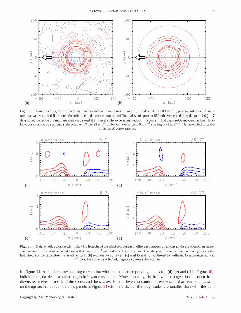
Figure 13. Contours of (a) vertical velocity (contour interval: thick lines 0.5 m s−1, thin dashed lines 0.1 m s−1, positive values solid lines,negative values dashed lines, the thin solid line is the zerocontour), and (b) total wind speed at 850 mb averaged during the period6 3

4− 7

days about the centre of minimum total wind speed at this level in the experiment withU = 5.0 m s−1 that uses the Gayno-Seaman boundary-layer parameterization scheme (thin contours 17 and 33 m s−1, thick contour interval 5 m s−1 starting at 45 m s−1). The arrow indicates the

direction of vortex motion.

(a) (b)

(c) (d)

Figure 14. Height-radius cross sections showing isotachs of the wind component in different compass directions (x) in the co-moving frame.The data are for the control calculation withU = 5 m s−1 and with the Gayno-Seaman boundary-layer scheme, and are averaged over thelast 6 hours of the calculation. (a) south to north, (b) southeast to northwest, (c) west to east, (d) southwest to northeast. Contour interval: 5 m

s−1. Positive contours solid/red, negative contours dashed/blue.

in Figure14. As in the corresponding calculation with thebulk scheme, the deepest and strongest inflow occurs on thedownstream (western) side of the vortex and the weakest ison the upstream side (compare the panels in Figure14with

the corresponding panels (c), (d), (e) and (f) in Figure10).More generally, the inflow is strongest in the sector fromnorthwest to south and weakest in that from southeast tonorth, but the magnitudes are smaller than with the bulk



scheme.

7 Conclusions

We have presented an analysis of low-level flow asym-metries in the prototype problem for the intensificationof a moving tropical cyclone using a three-dimensional,convection-permitting numerical model. The problem con-siders the evolution of an initially dry, axisymmetric vortexin hydrostatic and gradient wind balance, embedded in auniform zonal flow on anf -plane. The calculations weredesigned to examine the hypothesized effects of a uniformflow on the intensification, structural evolution, and matureintensity of a tropical cyclone. The calculations naturallycomplement those of Nguyenet al. (2008), who examinedthe processes of tropical-cyclone intensification in a quies-cent environment from an ensemble perspective, and theyprovide a bridge between this problem and the intensifi-cation problem in vertical shear. In particular, the paperaddresses three outstanding basic questions concerning theeffects of moist convection on the azimuthal flow asymme-tries.

The first question is: does the imposition of a uniformflow lead to an organization of the inner-core convectionmaking its distribution more predictable compared with thecase of a quiescent environment? The answer to this ques-tion is a qualified yes. For the relatively strong vorticesmostly studied here, the effect is pronounced only for back-ground flow speeds larger than about 7 m s−1. In such caseswe found that the time-averaged vertical velocity field at850 mb during the last six hours of the calculations has avortex-scale maximum at about 45o to the left of the vortexmotion vector. This maximum survives also in an ensemblemean of calculations in which the initial low-level moisturefield is perturbed. Therefore, we conclude that this maxi-mum is a robust feature and neither a transient one nor aproperty of a single realization associated with a particularmesoscale convective feature. In an Earth-relative frame,the total wind speed has a maximum in the forward rightquadrant, a feature that survives also in the ensemble meancalculation. In the co-moving frame, this maximum lies tothe left of the motion vector in the ensemble mean. Thelow-level asymmetric wind structure found above remainsunaltered when the more sophisticated, but more diffusiveGayno-Seaman scheme is used to represent the boundarylayer, suggesting that our results are not overly sensitivetothe boundary-layer scheme used.

The second question is: to what extent do our resultscorroborate with those of previous theoretical investiga-tions? A useful metric for comparing the results is via thevortex-scale pattern of vertical velocity at the top of theboundary layer. We find that the direction of the maximumvertical velocity is about 45o to the left of that predictedby Shapiro’s nonlinear model (1983), where the maximumis in the direction of motion. This difference may haveconsequences for the interpretations of observations, sinceShapiro’s results are frequently invoked as a theoretical

benchmark for characterizing the boundary-layer inducedvertical motion (e.g. Corbosiero and Molinari (2003, p375).The reason for the difference is presumably, at least inpart, because in our calculations, the vortex flow above theboundary layer is determined as part of a full solution forthe flow and not prescribed. In other words, the wind andpressure fields at the top of the boundary layer adjust sothat, in the quasi-steady state, deep convection ventilatesthe mass that exits the boundary layer. Despite the fore-going discrepancy, we would argue that Shapiro’s nonlin-ear model provides an acceptable zero-order description ofthe boundary-layer asymmetries that survive the transienteffects of deep convection.

The third question is: how well do the findings com-pare with recent observations of boundary-layer flow asym-metries in translating storms by Kepert (2006a,b) andSchwendike and Kepert (2008)? We found that verticalcross sections of the 6-hour averaged, storm-relative, tan-gential wind component in the lowest 3 kilometres duringthe mature stage show a slight tendency for the maximumtangential wind component to become lower in altitudewith decreasing radius as the radius of the maximum tan-gential wind is approached. Moreover, the storm-relativemaximum tangential wind speed occurs on the left (i.e.southern) side of the storm as is found in the observationsreported in the foregoing papers. Similar cross sectionsof the radial wind component show that the strongest anddeepest inflow occurs in the sector from northwest to south-west (for a storm moving westwards) and the weakest andshallowest inflow in the sector southeast to east, consistentalso with the observations. In contrast, the radial wind com-ponentat individual times during the mature stage showsconsiderable variability on a 15 minute time scale, appar-ently because of the variability of deep convection on thistime scale. This result raises a potential issue concerningthe ability to determine meaningful vortex-scale asymme-tries in the radial inflow from dropwindsonde observationsspread over several hours.

The ensemble calculations show that an increase inthe background flow leads to a slight reduction in theintensification rate and to a weaker storm after 7 days. Thereduction in mature intensity is on the order of 10 m s−1

from zero background flow to one of 12.5 m s−1, althoughthere are a few times when the reduction in intensity withbackground flow speed does not vary monotonically. Theresults on intensity reduction are broadly consistent withthe observational analysis presented by Zenget al. (2007),although we should caution that, because the ensemblespread of storm intensity in our model has a magnitude alsoon the order of 10 m s−1, a comparison of two particularensemble members for two different background flowsmay yield a different result to that of Zengetal. Further,we noted that the metric used here for intensity is basedon the maximumtotal wind speed at 850 mb, a metricthat is perhaps less suitable for theoretical analysis thanan azimuthal average of the tangential wind component.This is one reason we have not tried to offer a theoretical



explanation here for the effects of translation speed onthe intensification rate and mature intensity. A satisfactoryexplanation for this dependence remains a topic for futureresearch.

Acknowledgement

GLT and RKS were supported in part by GrantSM 30/23-1 from the German Research Council(DFG). MTM acknowledges the support of Grant No.N0001411Wx20095 from the U.S. Office of NavalResearch and NSF AGS-0733380 and NSF AGS-0851077,and NASA grants NNH09AK561 and NNG09HG031.

References

Black, P. G., et al., 2007: Air-sea exchange in hurricanes.Synthesis of observations from the coupled boundarylayer air-sea transfer experiment.Bull Amer. Meteor.Soc., 88, 357–374.

Braun, S. A. and W.-K. Tao, 2000: Sensitivity of high-resolution simulations of hurricane bob (1991) to plan-etary boundary layer parameterizations.Mon. Wea. Rev.,128, 3941–3961.

Bui, H. H., R. K. Smith, M. T. Montgomery, and J. Peng,2009: Balanced and unbalanced aspects of tropical-cyclone intensification.Quart. Journ. Roy. Meteor. Soc.,135, 1715–1731.

Corbosiero, K. L. and J. Molinari, 2002: The effects ofvertical wind shear on the distribution of convection intropical cyclones.Mon. Wea. Rev., 130, 2110–2123.

Corbosiero, K. L. and J. Molinari, 2003: The relationshipbetween storm motion, vertical wind shear, and convec-tive asymmetries in tropical cyclones.J. Atmos. Sci., 60,366–376.

Dudhia, J., 1993: A non-hydrostatic version of the PennState/NCAR mesoscale model: Validation tests and sim-ulation of an Atlantic cyclone and cold front.Mon. Wea.Rev., 121, 1493–1513.

Frank, W. M. and E. A. Ritchie, 1999: Effects of envi-ronmental flow on tropical cyclone structure.Mon. Wea.Rev., 127, 2044–2061.

Frank, W. M. and E. A. Ritchie, 2001: Effects of verticalwind shear on the intensity and structure of numericallysimulated hurricanes.Mon. Wea. Rev., 129, 2249–2269.

Grell, G. A., J. Dudhia, and D. R. Stauffer, 1995: Adescription of the fifth generation Penn State/NCARmesoscale model (MM5).NCAR Tech Note NCAR/TN-398+STR., 000, 138.

Jones, S. C., 1995: The evolution of vortices in verticalshear. Part I: Initially barotropic vortices.Quart. Journ.Roy. Meteor. Soc., 121, 821–851.

Jones, S. C., 2000: The evolution of vortices in verticalshear. III: Baroclinic vortices.Quart. Journ. Roy. Meteor.Soc., 126, 3161–3186.

Jordan, C. L., 1958: Mean soundings for the West Indiesarea.J. Meteor., 15, 91–97.

Kepert, J. D., 2001: The dynamics of boundary layer jetswithin the tropical cyclone core. Ppart I: Linear theory.J. Atmos. Sci., 58, 2469–2484.

Kepert, J. D., 2006a: Observed boundary-layer wind struc-ture and balance in the hurricane core. Part I. HurricaneGeorges.J. Atmos. Sci., 63, 2169–2193.

Kepert, J. D., 2006b: Observed boundary-layer wind struc-ture and balance in the hurricane core. Part II. HurricaneMitch. J. Atmos. Sci., 63, 2194–2211.

Kepert, J. D. and Y. Wang, 2001: The dynamics of bound-ary layer jets within the tropical cyclone core. Part II:Nonlinear enhancement.J. Atmos. Sci., 58, 2485–2501.

McIntyre, M. E., 1993: Isentropic distributions of potentialvorticity and their relevance to tropical cyclone dynam-ics. Tropical cyclone disasters, J. Lighthill, Z. Zhemin,G. Holland, and K. Emanuel, Eds., ICSU/WMO Interna-tional Symposium on Tropical Cyclone Disasters, Octo-ber 12-16, 1992, Beijing , China.

Montgomery, M. T., M. M. Bell, S. D. Aberson, and M. L.Black, 2006: Hurricane isabel (2003): New insightsinto the physics of intense storms. Part I mean vortexstructure and maximum intensity estimates.Bull Amer.Meteor. Soc., 87, 1335–1348.

Nguyen, V. S., R. K. Smith, and M. T. Montgomery,2008: Tropical-cyclone intensification and predictabilityin three dimensions.Quart. Journ. Roy. Meteor. Soc.,134, 563–582.

Powell, M. D., 1982: The transition of the hurricane fred-eric boundary layer wind field from the open gulf ofmexico to landfall.Mon. Wea. Rev., 110, 1912–1932.

Raymond, D. J., 1992: Nonlinear balance and potential-vorticity thinking at large rossby number.Quart. Journ.Roy. Meteor. Soc., 118, 987–1015.

Reasor, P. D. and M. T. Montgomery, 2004: Three-dimensional alignment and co-rotation of weak TC-likevortices via linear vortex rossby waves.J. Atmos. Sci.,58, 2306–2330.

Riemer, M., M. T. Montgomery, and M. E. Nicholls, 2010:A new paradigm for intensity modification of tropicalcyclones: Thermodynamic impact of vertical wind shearon the inflow layer.Atmos. Chem. Phys., 10, 3163–3188.



Rogers, R., S. Lorsolo, P. Reasor, J. Gamache, andF. Marks, 2012: Multiscale analysis of tropical cyclonekinematic structure from airborne doppler radar compos-ites.Mon. Wea. Rev., 140, 77–99.

Schwendike, J. and J. D. Kepert, 2008: The boundary layerwinds in Hurricane Danielle (1998) and Isabel (2003).Mon. Wea. Rev., 136, 3168–3192.

Shafran, P. C., N. L. Seaman, and G. A. Gayno, 2000:Evaluation of numerical predictions of boundary layerstructure during the lake michigan ozone study.J. Appl.Met., 39, 3168–3192.

Shapiro, L. J., 1983: The asymmetric boundary layer flowunder a translating hurricane.J. Atmos. Sci., 40, 1984–1998.

Shin, S. and R. K. Smith, 2008: Tropical-cyclone intensifi-cation and predictability in a minimal three-dimensionalmodel.Quart. Journ. Roy. Meteor. Soc., 134, 337–351.

Smith, R. K., 2006: Accurate determination of a balancedaxisymmetric vortex.Tellus, 58A, 98–103.

Smith, R. K., M. T. Montgomery, and S. V. Nguyen, 2009:Tropical cyclone spin up revisited.Quart. Journ. Roy.Meteor. Soc., 135, 1321–1335.

Smith, R. K. and G. L. Thomsen, 2010: Dependence oftropical-cyclone intensification on the boundary layerrepresentation in a numerical model.Quart. Journ. Roy.Meteor. Soc., 136, 1671–1685.

Smith, R. K., W. Ulrich, and G. Sneddon, 2000: On thedynamics of hurricane-like vortices in vertical shearflows.Quart. Journ. Roy. Meteor. Soc., 126, 2653–2670.

Weckwerth, T., 2000: The effect of small-scale moisturevariability on thunderstorm initiation.Mon. Wea. Rev.,128, 4017–4030.

Zeng, Z., Y. Wang, and C. C. Wu, 2011: Environmentaldynamical control of tropical cyclone intensity - anobservational study.Mon. Wea. Rev., 135, 38–59.

Zhang, J., W. M. Drennan, P. B. Black, and J. R. French,2009: Turbulence structure of the hurricane boundarylayer between the outer rainbands.J. Atmos. Sci., 66,2455–2467.

Zhang, J. A., F. D. Marks, M. T. Montgomery, and S. Lor-solo, 2011a: An estimation of turbulent characteristics inthe low-level region of intense Hurricanes Allen (1980)and Hugo (1989).Mon. Wea. Rev., 139, 1447–1462.

Zhang, J. A., R. F. Rogers, D. S. Nolan, and F. D. Marks,2011b: On the characteristic height scales of the hurri-cane boundary layer.Mon. Wea. Rev., 139, 2523–2535.

Zhang, J. A., R. F. Rogers, D. S. Nolan, and F. D. Marks,2013: Asymmetric hurricane boundary layer structurefrom dropsonde composites in relation to the environ-mental vertical wind shear.Mon. Wea. Rev., 141, 3968–3983.

Zhang, J. A. and E. Ulhorn, 2012: Hurricane sea surfaceinflow angle and an observation-based parametric model.Mon. Wea. Rev., 10, 3587–3605.


Documents

Tropical-cyclone flow asymmetries induced by a …roger/Publications/TCRR...Tropical-cyclone flow asymmetries induced by a uniform flow revisited ... b Dept. of Meteorology,