Embed Size (px)
Citation preview
French-Russian Laboratory “J.-V. Poncelet”Moscow Center for Continuous Mathematical Education
Independent University of MoscowInstitute for Information Transmission Problems of RAS
Institute of Control Sciences of RAS
International Workshop
TROPICAL AND IDEMPOTENTMATHEMATICS
Moscow, Russia, August 26–31, 2012
G. L. Litvinov, V. P. Maslov,
A. G. Kushner, S. N. Sergeev (Eds.)
Moscow – 2012
ISBN 978-5-91910-143-7
G. L. Litvinov, V. P. Maslov, A. G. Kushner, S. N. Sergeev(Eds.) Tropical and idempotent mathematics. – Moscow: 2012 – 276pages.
TEX editor: S. N. Tychkov.
This volume contains the proceedings of the International Workshopon Idempotent and Tropical Mathematics (Moscow, Russia, August26–31, 2012).This publication is supported by the RFBR grant 12-01-06083-g.
2000 Mathematics Subject Classification: 00B10, 81Q20, 06F07,35Q99, 49L90, 46S99, 81S99, 52B20,52A41, 14P99.
c⃝2012 by Institute for Information Transmission Problems of RAS.
PREFACE
Idempotent/tropical mathematics is a relatively new branch of mathemat-ical sciences, which rapidly developed and gained popularity over the last twodecades. It is closely related to many areas of mathematics and numerous appli-cations. Tropical mathematics is a very imporatant part of idempotent mathe-matics, see an introductory lecture below. The literature on the subject is vastand includes numerous books and an all but innumerable body of journal papers.
The present book contains materials presented for the International Work-shop TROPICAL AND IDEMPOTENT MATHEMATICS, Moscow, Russia, Au-gust 26–31, 2012. Our workshop has become traditional. Materials related withprevious workshops are presented in volumes 377 and 495 of ContemporaryMathematics (American Mathematical Society, Providence, Rhode Island, 2005and 2009).
It is our pleasure to thank all the institutions supporting the workshop: theIndependent University of Moscow, French-Russian Laboratory "J.V. Poncelet",Moscow Center for Continuous Mathematical Education, A.A. Kharkevich Insti-tute for Information Transmission Problems of RAS, V.A. Trapeznikov Instituteof Control Sciences of RAS, Russian Fund for Basic Research, CNRS (France),and Dynasty Fund (Moscow), for their important support.
We are grateful to a number of colleagues, especially to E.S. Kryukova, A. P.Kuleshov, A.N. Sobolevski, and M.A. Tsfasman, for their great help. We thank allthe authors of the volume and members of our "idempotent/max-plus, tropicalcommunity" for their contributions, help, useful contacts and discussions.
The editorsMoscow, August 2012.

Tropical and Idempotent Mathematics. Moscow, Russia, August 26–31, 2012
Dequantization of mathematical structures andtropical/idempotent mathematics. An introduc-tory lecture
G. L. Litvinov
Abstract A very brief introduction to tropical and idempotent mathematics ispresented.
1 Introduction
Tropical mathematics can be treated as a result of a dequantization of the tradi-tional mathematics as the Planck constant tends to zero taking imaginary values.This kind of dequantization is known as the Maslov dequantization and it leadsto a mathematics over tropical algebras like the max-plus algebra. The so-calledidempotent dequantization is a generalization of the Maslov dequantization. Theidempotent dequantization leads to mathematics over idempotent semirings (ex-act definitions see below in sections 2 and 3). For example, the field of real orcomplex numbers can be treated as a quantum object whereas idempotent semir-ings can be examined as "classical" or "semiclassical" objects (a semiring is calledidempotent if the semiring addition is idempotent, i.e. x⊕ x = x), see [9–13].
Tropical algebras are idempotent semirings (and semifields). Thus tropicalmathematics is a part of idempotent mathematics. Tropical algebraic geometrycan be treated as a result of the Maslov dequantization applied to the traditional
6 G. L. Litvinov
semirings andsemifields
QUANTUMMECHANICS
MATHEMATICSTRADITIONAL
numbersreal and complex
Fields of
N. Bohr’s Correspondence Principle
Idempotent Correspondence Principle
CLASSICALMECHANICS
IDEMPOTENTMATHEMATICS
Idempotent
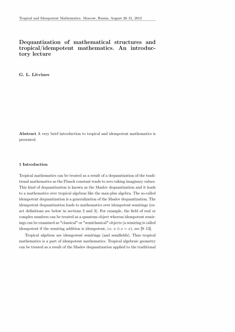
Fig. 1 Relations between idempotent and traditional mathematics.
algebraic geometry (O. Viro, G. Mikhalkin), see, e.g., [7,34,35,38–40]. There areinteresting relations and applications to the traditional convex geometry.
In the spirit of N.Bohr’s correspondence principle there is a (heuristic) cor-respondence between important, useful, and interesting constructions and re-sults over fields and similar results over idempotent semirings. A systematicapplication of this correspondence principle (which is a basic paradigm in idem-potent/tropical mathematcs) leads to a variety of theoretical and applied re-sults [9–14,20], see Fig.1.
The history of the subject is discussed, e.g., in [9]. There is a large list ofreferences.
2 The Maslov dequantization
Let R and C be the fields of real and complex numbers. The so-called max-plusalgebra Rmax = R ∪ −∞ is defined by the operations x⊕ y = maxx, y andx⊙ y = x+ y.
The max-plus algebra can be treated as a result of the Maslov dequantizationof the semifield R+ of all nonnegative numbers with the usual arithmetics. Thechange of variables
x 7→ u = h log x,
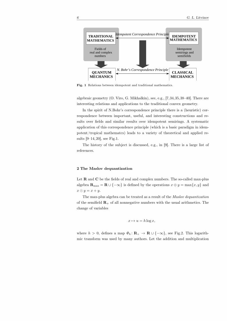
where h > 0, defines a map Φh : R+ → R ∪ −∞, see Fig.2. This logarith-mic transform was used by many authors. Let the addition and multiplication
Dequantization of mathematical structures and tropical/idempotent mathematics 7
u
0 1 +RÎu
Rmax(h)
Îw
11
¥ = 0
w= lnh u
w
Fig. 2 Deformation of R+ to R(h). Inset: the same for a small value of h.
operations be mapped from R+ to R ∪ −∞ by Φh, i.e. let
u⊕h v = h log(exp(u/h) + exp(v/h)), u⊙ v = u+ v,
0 = −∞ = Φh(0), 1 = 0 = Φh(1).
It can easily be checked that u⊕h v → maxu, v as h→ 0. Thus we get thesemifield Rmax (i.e. the max-plus algebra) with zero 0 = −∞ and unit 1 = 0 asa result of this deformation of the algebraic structure in R+.
The semifield Rmax is a typical example of an idempotent semiring; this isa semiring with idempotent addition, i.e., x ⊕ x = x for arbitrary element x ofthis semiring.
The semifield Rmax is also called a tropical algebra.The semifield R(h) =
Φh(R+) with operations ⊕h and ⊙ (i.e.+) is called a subtropical algebra.The semifield Rmin = R ∪ +∞ with operations ⊕ = min and ⊙ = +
(0 = +∞,1 = 0) is isomorphic to Rmax.
8 G. L. Litvinov
The analogy with quantization is obvious; the parameter h plays the role ofthe Planck constant. The map x 7→ |x| and the Maslov dequantization for R+
give us a natural transition from the field C (or R) to the max-plus algebraRmax. We will also call this transition the Maslov dequantization. In fact theMaslov dequantization corresponds to the usual Schrodinger dequantization butfor imaginary values of the Planck constant (see below). The transition fromnumerical fields to the max-plus algebra Rmax (or similar semifields) in mathe-matical constructions and results generates the so called tropical mathematics.The so-called idempotent dequantization is a generalization of the Maslov de-quantization; this is the transition from basic fields to idempotent semirings inmathematical constructions and results without any deformation. The idempo-tent dequantization generates the so-called idempotent mathematics, i.e. math-ematics over idempotent semifields and semirings. Recently new versions of theMaslov dequantization appeared, see, e.g. [41].
Remark. The term ’tropical’ appeared in [37] for a discrete version of themax-plus algebra (as a suggestion of Christian Choffrut). On the other hand V.P.Maslov used this term in 80s in his talks and works on economical applicationsof his idempotent analysis (related to colonial politics). For the most part ofmodern authors, ’tropical’ means ’over Rmax (or Rmin)’ and tropical algebrasare Rmax and Rmin. The terms ’max-plus’, ’max-algebra’ and ’min-plus’ areoften used in the same sense.
3 Semirings and semifields
Consider a set S equipped with two algebraic operations: addition ⊕ and multi-plication ⊙. It is a semiring if the following conditions are satisfied:
– the addition ⊕ and the multiplication ⊙ are associative;– the addition ⊕ is commutative;– the multiplication ⊙ is distributive with respect to the addition ⊕:
x⊙ (y ⊕ z) = (x⊙ y)⊕ (x⊙ z)
and
(x⊕ y)⊙ z = (x⊙ z)⊕ (y ⊙ z)
for all x, y, z ∈ S.
A unity of a semiring S is an element 1 ∈ S such that 1 ⊙ x = x ⊙ 1 = x forall x ∈ S. A zero of a semiring S is an element (if it exists) 0 ∈ S such that
Dequantization of mathematical structures and tropical/idempotent mathematics 9
0 = 1 and 0 ⊕ x = x, 0 ⊙ x = x ⊙ 0 = 0 for all x ∈ S. A semiring S is calledan idempotent semiring if x⊕ x = x for all x ∈ S. A semiring S with a neutralelement 1 is called a semifield if every nonzero element of S is invertible withrespect to the multiplication. The theory of semirings and semifields is treated,e.g., in [5].
4 Idempotent analysis
Idempotent analysis deals with functions taking their values in an idempotentsemiring and the corresponding function spaces. Idempotent analysis was ini-tially constructed by V. P. Maslov and his collaborators and then developed bymany authors. The subject is presented in the book of V. N. Kolokoltsov andV. P. Maslov [8] (a version of this book in Russian was published in 1994).
Let S be an arbitrary semiring with idempotent addition ⊕ (which is alwaysassumed to be commutative), multiplication ⊙, and unit 1. The set S is suppliedwith the standard partial order ≼: by definition, a ≼ b if and only if a ⊕ b = b.If the zero element exists, then all elements of S are nonnegative: 0 ≼ a for alla ∈ S. Due to the existence of this order, idempotent analysis is closely relatedto the lattice theory, theory of vector lattices, and theory of ordered spaces.Moreover, this partial order allows to model a number of basic “topological”concepts and results of idempotent analysis at the purely algebraic level; thisline of reasoning was examined systematically in [9]– [24] and [3].
Calculus deals mainly with functions whose values are numbers. The idem-potent analog of a numerical function is a map X → S, where X is an arbitraryset and S is an idempotent semiring. Functions with values in S can be added,multiplied by each other, and multiplied by elements of S pointwise.
The idempotent analog of a linear functional space is a set of S-valued func-tions that is closed under addition of functions and multiplication of functions byelements of S, or an S-semimodule. Consider, e.g., the S-semimodule B(X,S)
of all functions X → S that are bounded in the sense of the standard order onS.
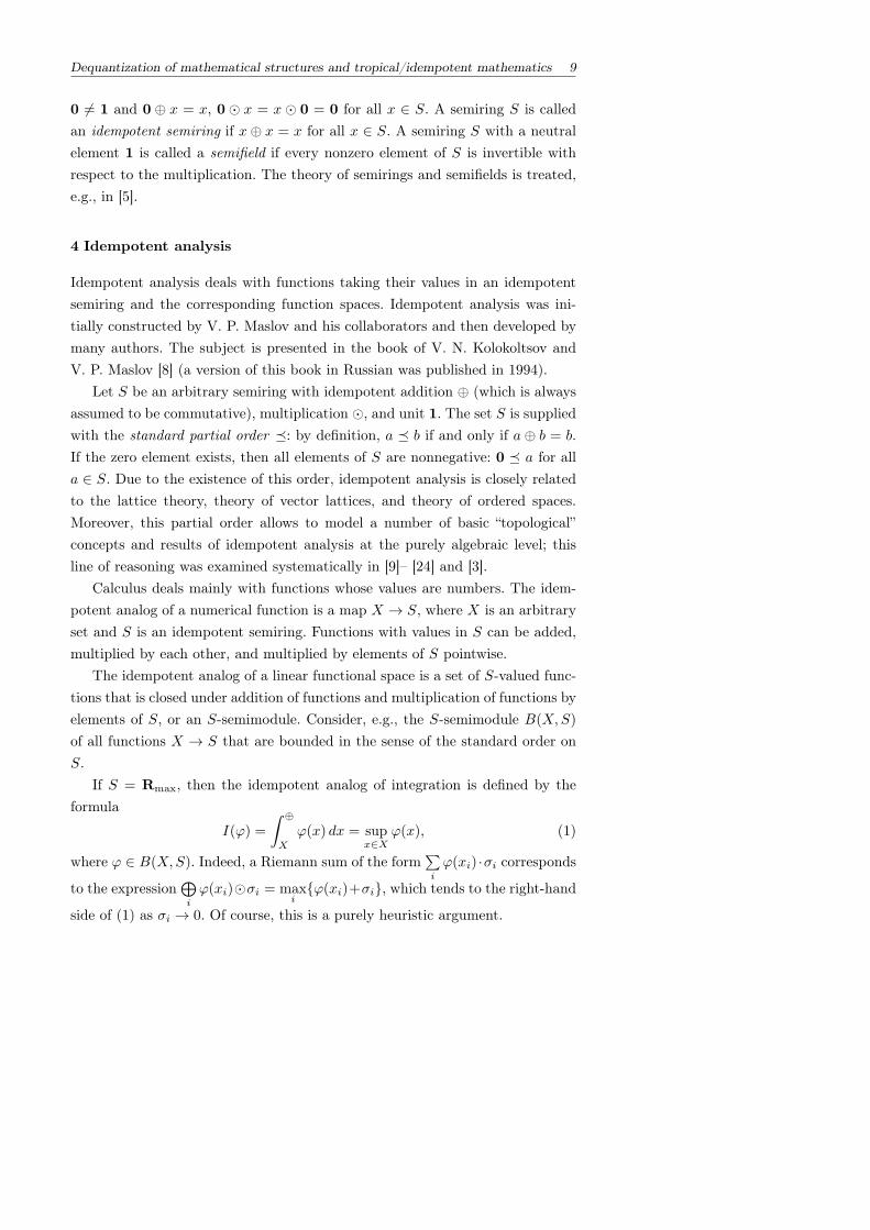
If S = Rmax, then the idempotent analog of integration is defined by theformula
I(φ) =
∫ ⊕
X
φ(x) dx = supx∈X
φ(x), (1)
where φ ∈ B(X,S). Indeed, a Riemann sum of the form∑i
φ(xi) ·σi corresponds
to the expression⊕i
φ(xi)⊙σi = maxi
φ(xi)+σi, which tends to the right-hand
side of (1) as σi → 0. Of course, this is a purely heuristic argument.
10 G. L. Litvinov
Formula (1) defines the idempotent (or Maslov) integral not only for functionstaking values in Rmax, but also in the general case when any of bounded (fromabove) subsets of S has the least upper bound.
An idempotent (or Maslov) measure on X is defined by the formula mψ(Y ) =
supx∈Y
ψ(x), where ψ ∈ B(X,S) is a fixed function. The integral with respect to
this measure is defined by the formula
Iψ(φ) =
∫ ⊕
X
φ(x) dmψ =
∫ ⊕
X
φ(x)⊙ ψ(x) dx = supx∈X
(φ(x)⊙ ψ(x)). (2)
Obviously, if S = Rmin, then the standard order is opposite to the conven-tional order ≤, so in this case equation (2) assumes the form∫ ⊕
X
φ(x) dmψ =
∫ ⊕
X
φ(x)⊙ ψ(x) dx = infx∈X
(φ(x)⊙ ψ(x)),
where inf is understood in the sense of the conventional order ≤.
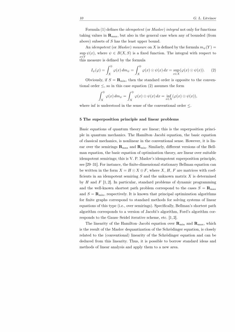
5 The superposition principle and linear problems
Basic equations of quantum theory are linear; this is the superposition princi-ple in quantum mechanics. The Hamilton–Jacobi equation, the basic equationof classical mechanics, is nonlinear in the conventional sense. However, it is lin-ear over the semirings Rmax and Rmin. Similarly, different versions of the Bell-man equation, the basic equation of optimization theory, are linear over suitableidempotent semirings; this is V. P. Maslov’s idempotent superposition principle,see [29–31]. For instance, the finite-dimensional stationary Bellman equation canbe written in the form X = H ⊙X ⊕F , where X, H, F are matrices with coef-ficients in an idempotent semiring S and the unknown matrix X is determinedby H and F [1, 2]. In particular, standard problems of dynamic programmingand the well-known shortest path problem correspond to the cases S = Rmax
and S = Rmin, respectively. It is known that principal optimization algorithmsfor finite graphs correspond to standard methods for solving systems of linearequations of this type (i.e., over semirings). Specifically, Bellman’s shortest pathalgorithm corresponds to a version of Jacobi’s algorithm, Ford’s algorithm cor-responds to the Gauss–Seidel iterative scheme, etc. [1, 2].
The linearity of the Hamilton–Jacobi equation over Rmin and Rmax, whichis the result of the Maslov dequantization of the Schrodinger equation, is closelyrelated to the (conventional) linearity of the Schrodinger equation and can bededuced from this linearity. Thus, it is possible to borrow standard ideas andmethods of linear analysis and apply them to a new area.
Dequantization of mathematical structures and tropical/idempotent mathematics 11
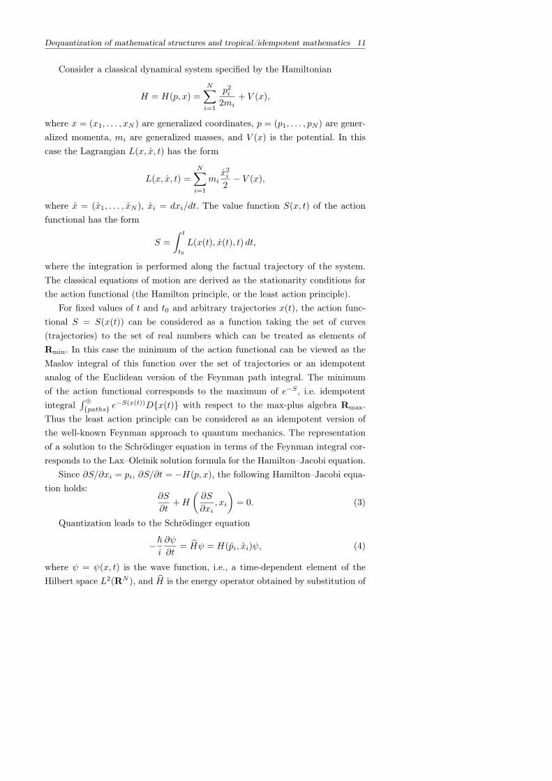
Consider a classical dynamical system specified by the Hamiltonian
H = H(p, x) =N∑i=1
p2i2mi
+ V (x),
where x = (x1, . . . , xN ) are generalized coordinates, p = (p1, . . . , pN ) are gener-alized momenta, mi are generalized masses, and V (x) is the potential. In thiscase the Lagrangian L(x, x, t) has the form
L(x, x, t) =N∑i=1
mix2i2
− V (x),
where x = (x1, . . . , xN ), xi = dxi/dt. The value function S(x, t) of the actionfunctional has the form
S =
∫ t
t0
L(x(t), x(t), t) dt,
where the integration is performed along the factual trajectory of the system.The classical equations of motion are derived as the stationarity conditions forthe action functional (the Hamilton principle, or the least action principle).
For fixed values of t and t0 and arbitrary trajectories x(t), the action func-tional S = S(x(t)) can be considered as a function taking the set of curves(trajectories) to the set of real numbers which can be treated as elements ofRmin. In this case the minimum of the action functional can be viewed as theMaslov integral of this function over the set of trajectories or an idempotentanalog of the Euclidean version of the Feynman path integral. The minimumof the action functional corresponds to the maximum of e−S , i.e. idempotentintegral
∫ ⊕paths e
−S(x(t))Dx(t) with respect to the max-plus algebra Rmax.Thus the least action principle can be considered as an idempotent version ofthe well-known Feynman approach to quantum mechanics. The representationof a solution to the Schrodinger equation in terms of the Feynman integral cor-responds to the Lax–Oleınik solution formula for the Hamilton–Jacobi equation.
Since ∂S/∂xi = pi, ∂S/∂t = −H(p, x), the following Hamilton–Jacobi equa-tion holds:
∂S
∂t+H
(∂S
∂xi, xi
)= 0. (3)
Quantization leads to the Schrodinger equation
−~i
∂ψ
∂t= Hψ = H(pi, xi)ψ, (4)
where ψ = ψ(x, t) is the wave function, i.e., a time-dependent element of theHilbert space L2(RN ), and H is the energy operator obtained by substitution of
12 G. L. Litvinov
the momentum operators pi = ~i∂∂xi
and the coordinate operators xi : ψ 7→ xiψ
for the variables pi and xi in the Hamiltonian function, respectively. This equa-tion is linear in the conventional sense (the quantum superposition principle).The standard procedure of limit transition from the Schrodinger equation to theHamilton–Jacobi equation is to use the following ansatz for the wave function:ψ(x, t) = a(x, t)eiS(x,t)/~, and to keep only the leading order as ~ → 0 (the‘semiclassical’ limit).
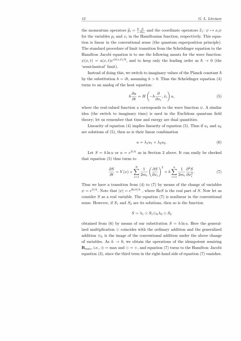
Instead of doing this, we switch to imaginary values of the Planck constant ~by the substitution h = i~, assuming h > 0. Thus the Schrodinger equation (4)turns to an analog of the heat equation:
h∂u
∂t= H
(−h ∂
∂xi, xi
)u, (5)
where the real-valued function u corresponds to the wave function ψ. A similaridea (the switch to imaginary time) is used in the Euclidean quantum fieldtheory; let us remember that time and energy are dual quantities.
Linearity of equation (4) implies linearity of equation (5). Thus if u1 and u2are solutions of (5), then so is their linear combination
u = λ1u1 + λ2u2. (6)
Let S = h lnu or u = eS/h as in Section 2 above. It can easily be checkedthat equation (5) thus turns to
∂S
∂t= V (x) +
N∑i=1
1
2mi
(∂S
∂xi
)2
+ h
n∑i=1
1
2mi
∂2S
∂x2i. (7)
Thus we have a transition from (4) to (7) by means of the change of variablesψ = eS/h. Note that |ψ| = eReS/h , where ReS is the real part of S. Now let usconsider S as a real variable. The equation (7) is nonlinear in the conventionalsense. However, if S1 and S2 are its solutions, then so is the function
S = λ1 ⊙ S1⊕hλ2 ⊙ S2
obtained from (6) by means of our substitution S = h lnu. Here the general-ized multiplication ⊙ coincides with the ordinary addition and the generalizedaddition ⊕h is the image of the conventional addition under the above changeof variables. As h → 0, we obtain the operations of the idempotent semiringRmax, i.e., ⊕ = max and ⊙ = +, and equation (7) turns to the Hamilton–Jacobiequation (3), since the third term in the right-hand side of equation (7) vanishes.
Dequantization of mathematical structures and tropical/idempotent mathematics 13
Thus it is natural to consider the limit function S = λ1 ⊙ S1 ⊕ λ2 ⊙ S2 asa solution of the Hamilton–Jacobi equation and to expect that this equationcan be treated as linear over Rmax. This argument (clearly, a heuristic one) canbe extended to equations of a more general form. For a rigorous treatment of(semiring) linearity for these equations see, e.g., [8, 14, 36]. Notice that if h ischanged to −h, then we have that the resulting Hamilton–Jacobi equation islinear over Rmin.
The idempotent superposition principle indicates that there exist importantnonlinear (in the traditional sense) problems that are linear over idempotentsemirings. The idempotent linear functional analysis (see below) is a natural toolfor investigation of those nonlinear infinite-dimensional problems that possessthis property.
6 Convolution and the Fourier–Legendre transform
Let G be a group. Then the space B(G,Rmax) of all bounded functions G →Rmax (see above) is an idempotent semiring with respect to the following analog~ of the usual convolution:
(φ(x)~ ψ)(g) ==
∫ ⊕
G
φ(x)⊙ ψ(x−1 · g) dx = supx∈G
(φ(x) + ψ(x−1 · g)).
Of course, it is possible to consider other “function spaces” (and other basicsemirings instead of Rmax).
Let G = Rn, where Rn is considered as a topological group with respect tothe vector addition. The conventional Fourier–Laplace transform is defined as
φ(x) 7→ φ(ξ) =
∫G
eiξ·xφ(x) dx, (8)
where eiξ·x is a character of the groupG, i.e., a solution of the following functionalequation:
f(x+ y) = f(x)f(y).
The idempotent analog of this equation is
f(x+ y) = f(x)⊙ f(y) = f(x) + f(y),
so “continuous idempotent characters” are linear functionals of the form x 7→ξ · x = ξ1x1 + · · ·+ ξnxn. As a result, the transform in (8) assumes the form
φ(x) 7→ φ(ξ) =
∫ ⊕
G
ξ · x⊙ φ(x) dx = supx∈G
(ξ · x+ φ(x)). (9)
14 G. L. Litvinov
The transform in (9) is nothing but the Legendre transform (up to some no-tation) [31]; transforms of this kind establish the correspondence between theLagrangian and the Hamiltonian formulations of classical mechanics. The Leg-endre transform generates an idempotent version of harmonic analysis for thespace of convex functions, see, e.g., [27].
Of course, this construction can be generalized to different classes of groupsand semirings. Transformations of this type convert the generalized convolution~ to the pointwise (generalized) multiplication and possess analogs of someimportant properties of the usual Fourier transform.
The examples discussed in this sections can be treated as fragments of anidempotent version of the representation theory, see, e.g., [19, 26]. In particu-lar, “idempotent” representations of groups and semigroups can be examinedas representations of the corresponding convolution semirings (i.e. idempotent(semi)group semirings) in semimodules.
7 Idempotent functional analysis
Many other idempotent analogs may be given, in particular, for basic construc-tions and theorems of functional analysis. Idempotent functional analysis is anabstract version of idempotent analysis. For the sake of simplicity take S = Rmax
and let X be an arbitrary set. The idempotent integration can be defined by theformula (1), see above. The functional I(φ) is linear over S and its values corre-spond to limiting values of the corresponding analogs of Lebesgue (or Riemann)sums. An idempotent scalar product of functions φ and ψ is defined by theformula
⟨φ,ψ⟩ =∫ ⊕
X
φ(x)⊙ ψ(x) dx = supx∈X
(φ(x)⊙ ψ(x)).
So it is natural to construct idempotent analogs of integral operators in the form
φ(y) 7→ (Kφ)(x) =
∫ ⊕
Y
K(x, y)⊙ φ(y) dy = supy∈Y
K(x, y) + φ(y), (10)
where φ(y) is an element of a space of functions defined on a set Y , and K(x, y) isan S-valued function on X ×Y . Of course, expressions of this type are standardin optimization problems.
Recall that the definitions and constructions described above can be ex-tended to the case of idempotent semirings which are conditionally complete inthe sense of the standard order. Using the Maslov integration, one can construct
Dequantization of mathematical structures and tropical/idempotent mathematics 15
various function spaces as well as idempotent versions of the theory of gener-alized functions (distributions). For some concrete idempotent function spacesit was proved that every ‘good’ linear operator (in the idempotent sense) canbe presented in the form (10); this is an idempotent version of the kernel the-orem of L. Schwartz; results of this type were proved by V. N. Kolokoltsov,P. S. Dudnikov and S. N. Samborskiı, I. Singer, M. A. Shubin and others. Soevery ‘good’ linear functional can be presented in the form φ 7→ ⟨φ,ψ⟩, where⟨, ⟩ is an idempotent scalar product.
In the framework of idempotent functional analysis results of this type canbe proved in a very general situation. In [16–19, 22, 24] an algebraic version ofthe idempotent functional analysis is developed; this means that basic (topolog-ical) notions and results are simulated in purely algebraic terms. The treatmentcovers the subject from basic concepts and results (e.g., idempotent analogs ofthe well-known theorems of Hahn-Banach, Riesz, and Riesz-Fisher) to idem-potent analogs of A. Grothendieck’s concepts and results on topological tensorproducts, nuclear spaces and operators. Abstract idempotent versions of thekernel theorem is formulated. Note that the passage from the usual theory toidempotent functional analysis may be very nontrivial; for example, there aremany non-isomorphic idempotent Hilbert spaces. Important results on idem-potent functional analysis (duality and separation theorems) were obtained byG. Cohen, S. Gaubert, and J.-P. Quadrat. Idempotent functional analysis hasreceived much attention in the last years, see, e.g., [3], [8]– [24] and works citedin [9].
8 The dequantization transform and the Newton polytopes
Let X be a topological space. For functions f(x) defined on X we shall say thata certain property is valid almost everywhere (a.e.) if it is valid for all elementsx of an open dense subset of X. Suppose X is Cn or Rn; denote by Rn
+ the setx = (x1, . . . , xn) ∈ X | xi ≥ 0 for i = 1, 2, . . . , n. For x = (x1, . . . , xn) ∈ X weset exp(x) = (exp(x1), . . . , exp(xn)); so if x ∈ Rn, then exp(x) ∈ Rn
+.Denote by F(Cn) the set of all functions defined and continuous on an open
dense subset U ⊂ Cn such that U ⊃ Rn+. It is clear that F(Cn) is a ring (and
an algebra over C) with respect to the usual addition and multiplications offunctions.
For f ∈ F(Cn) let us define the function fh by the following formula:
fh(x) = h log |f(exp(x/h))|, (11)
16 G. L. Litvinov
where h is a (small) real positive parameter and x ∈ Rn. Set
f(x) = limh→+0
fh(x), (12)
if the right-hand side of (12) exists almost everywhere.We shall say that the function f(x) is a dequantization of the function f(x)
and the map f(x) 7→ f(x) is a dequantization transform. By construction, fh(x)and f(x) can be treated as functions taking their values in Rmax. Note that infact fh(x) and f(x) depend on the restriction of f to Rn
+ only; so in fact thedequantization transform is constructed for functions defined on Rn
+ only. It isclear that the dequantization transform is generated by the Maslov dequantiza-tion and the map x 7→ |x|.
Of course, similar definitions can be given for functions defined on Rn andRn
+. If s = 1/h, then we have the following version of (11) and (12):
f(x) = lims→∞
(1/s) log |f(esx)|. (12′)
Denote by ∂f the subdifferential of the function f at the origin.If f is a polynomial or if f is a sublinear function we have
∂f = v ∈ Rn | (v, x) ≤ f(x) ∀x ∈ Rn . (1)
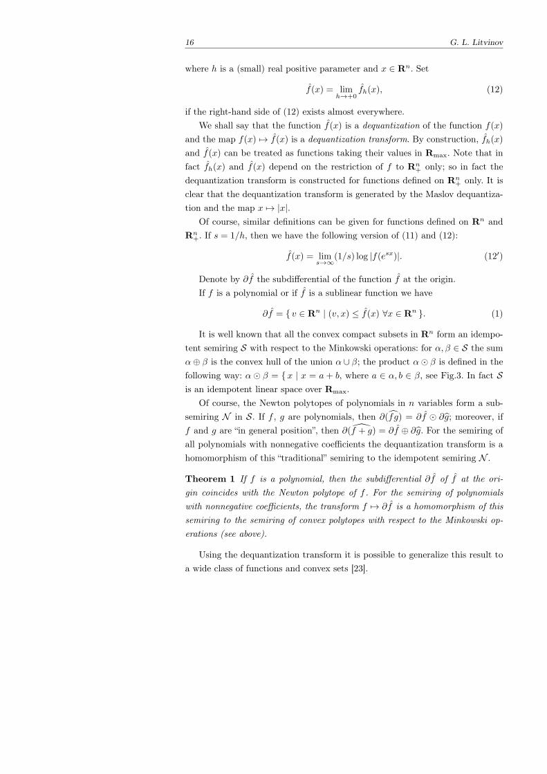
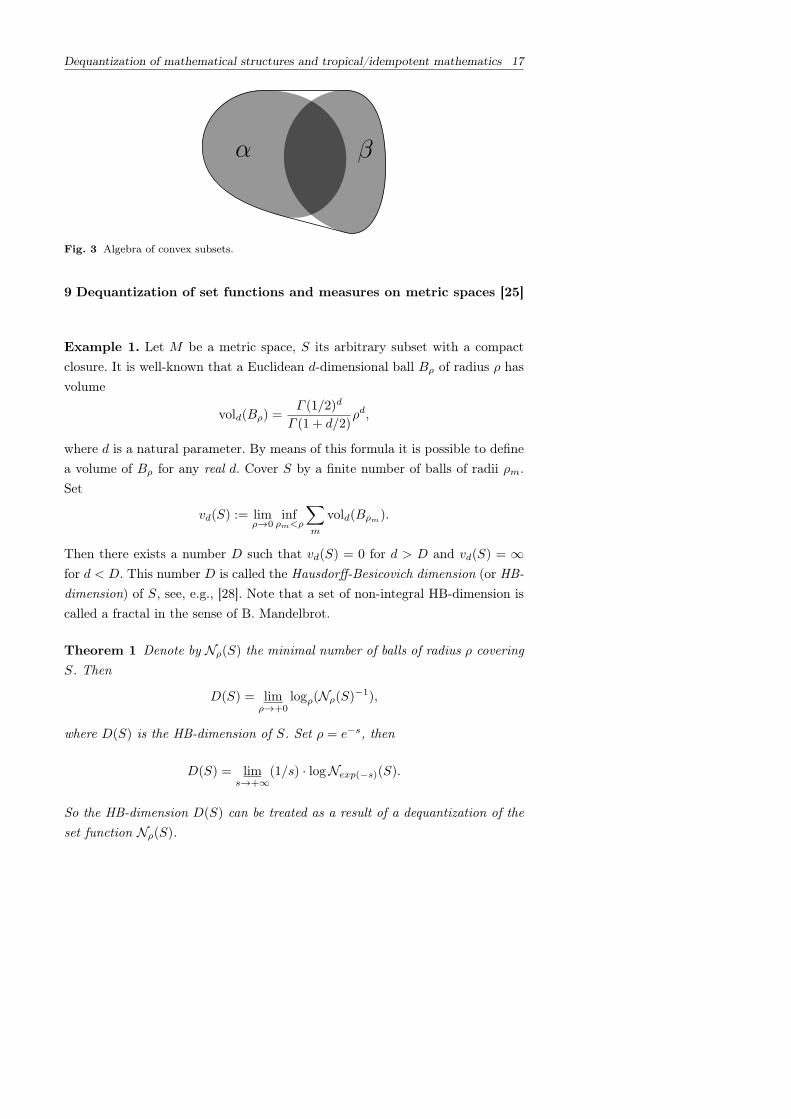
It is well known that all the convex compact subsets in Rn form an idempo-tent semiring S with respect to the Minkowski operations: for α, β ∈ S the sumα⊕ β is the convex hull of the union α ∪ β; the product α⊙ β is defined in thefollowing way: α ⊙ β = x | x = a + b, where a ∈ α, b ∈ β, see Fig.3. In fact Sis an idempotent linear space over Rmax.
Of course, the Newton polytopes of polynomials in n variables form a sub-semiring N in S. If f , g are polynomials, then ∂(fg) = ∂f ⊙ ∂g; moreover, iff and g are “in general position”, then ∂(f + g) = ∂f ⊕ ∂g. For the semiring ofall polynomials with nonnegative coefficients the dequantization transform is ahomomorphism of this “traditional” semiring to the idempotent semiring N .
Theorem 1 If f is a polynomial, then the subdifferential ∂f of f at the ori-gin coincides with the Newton polytope of f . For the semiring of polynomialswith nonnegative coefficients, the transform f 7→ ∂f is a homomorphism of thissemiring to the semiring of convex polytopes with respect to the Minkowski op-erations (see above).
Using the dequantization transform it is possible to generalize this result toa wide class of functions and convex sets [23].
Dequantization of mathematical structures and tropical/idempotent mathematics 17
α β
Fig. 3 Algebra of convex subsets.
9 Dequantization of set functions and measures on metric spaces [25]
Example 1. Let M be a metric space, S its arbitrary subset with a compactclosure. It is well-known that a Euclidean d-dimensional ball Bρ of radius ρ hasvolume
vold(Bρ) =Γ (1/2)d
Γ (1 + d/2)ρd,
where d is a natural parameter. By means of this formula it is possible to definea volume of Bρ for any real d. Cover S by a finite number of balls of radii ρm.Set
vd(S) := limρ→0
infρm<ρ
∑m
vold(Bρm).
Then there exists a number D such that vd(S) = 0 for d > D and vd(S) = ∞for d < D. This number D is called the Hausdorff-Besicovich dimension (or HB-dimension) of S, see, e.g., [28]. Note that a set of non-integral HB-dimension iscalled a fractal in the sense of B. Mandelbrot.
Theorem 1 Denote by Nρ(S) the minimal number of balls of radius ρ coveringS. Then
D(S) = limρ→+0
logρ(Nρ(S)−1),
where D(S) is the HB-dimension of S. Set ρ = e−s, then
D(S) = lims→+∞
(1/s) · logNexp(−s)(S).
So the HB-dimension D(S) can be treated as a result of a dequantization of theset function Nρ(S).
18 G. L. Litvinov
Example 2. Let µ be a set function on M (e.g., a probability measure) andsuppose that µ(Bρ) <∞ for every ball Bρ. Let Bx,ρ be a ball of radius ρ havingthe point x ∈M as its center. Then define µx(ρ) := µ(Bx,ρ) and let ρ = e−s and
Dx,µ := lims→+∞
−(1/s) · log(|µx(e−s)|).
This number could be treated as a dimension of M at the point x with respectto the set function µ. So this dimension is a result of a dequantization of thefunction µx(ρ), where x is fixed. There are many dequantization procedures ofthis type in different mathematical areas. In particular, V.P. Maslov’s negativedimension (see [32]) can be treated similarly.
10 Dequantization of geometry
An idempotent version of real algebraic geometry was discovered in the report ofO. Viro for the Barcelona Congress [38]. Starting from the idempotent correspon-dence principle O. Viro constructed a piecewise-linear geometry of polyhedra ofa special kind in finite dimensional Euclidean spaces as a result of the Maslovdequantization of real algebraic geometry. He indicated important applicationsin real algebraic geometry (e.g., in the framework of Hilbert’s 16th problemfor constructing real algebraic varieties with prescribed properties and parame-ters) and relations to complex algebraic geometry and amoebas in the sense ofI. M. Gelfand, M. M. Kapranov, and A. V. Zelevinsky, see [4,39]. Then complexalgebraic geometry was dequantized by G. Mikhalkin and the result turned outto be the same; this new ‘idempotent’ (or asymptotic) geometry is now oftencalled the tropical algebraic geometry, see, e.g., [7, 14,15,21,34,35].
There is a natural relation between the Maslov dequantization and amoebas.Suppose (C∗)n is a complex torus, where C∗ = C\0 is the group of nonzero
complex numbers under multiplication. For z = (z1, . . . , zn) ∈ (C∗)n and apositive real number h denote by Logh(z) = h log(|z|) the element
(h log |z1|, h log |z2|, . . . , h log |zn|) ∈ Rn.
Suppose V ⊂ (C∗)n is a complex algebraic variety; denote by Ah(V ) the setLogh(V ). If h = 1, then the set A(V ) = A1(V ) is called the amoeba of V ; theamoeba A(V ) is a closed subset of Rn with a non-empty complement. Note thatthis construction depends on our coordinate system.
For the sake of simplicity suppose V is a hypersurface in (C∗)n defined by apolynomial f ; then there is a deformation h 7→ fh of this polynomial generatedby the Maslov dequantization and fh = f for h = 1. Let Vh ⊂ (C∗)n be the
Dequantization of mathematical structures and tropical/idempotent mathematics 19
(a) (c)(b)
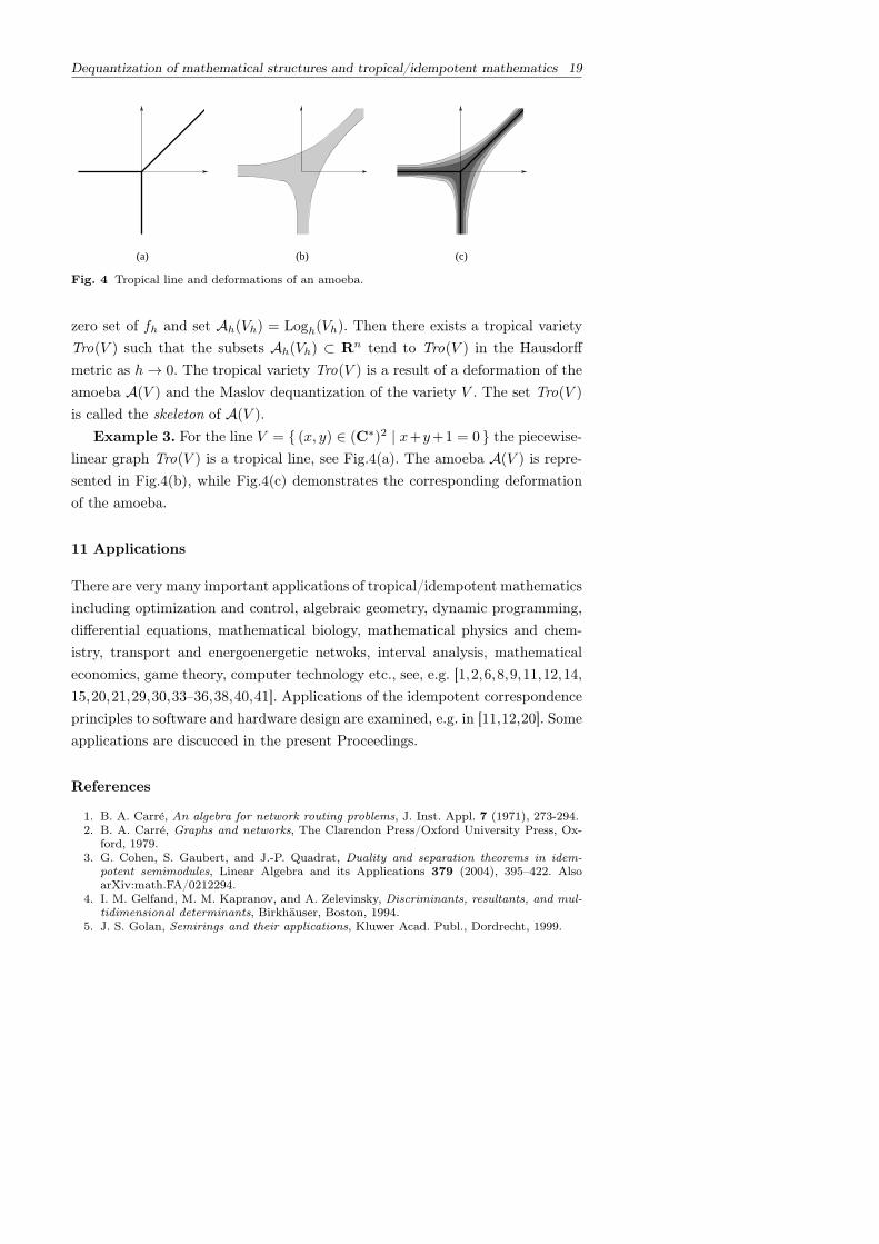
Fig. 4 Tropical line and deformations of an amoeba.
zero set of fh and set Ah(Vh) = Logh(Vh). Then there exists a tropical varietyTro(V ) such that the subsets Ah(Vh) ⊂ Rn tend to Tro(V ) in the Hausdorffmetric as h→ 0. The tropical variety Tro(V ) is a result of a deformation of theamoeba A(V ) and the Maslov dequantization of the variety V . The set Tro(V )
is called the skeleton of A(V ).Example 3. For the line V = (x, y) ∈ (C∗)2 | x+y+1 = 0 the piecewise-
linear graph Tro(V ) is a tropical line, see Fig.4(a). The amoeba A(V ) is repre-sented in Fig.4(b), while Fig.4(c) demonstrates the corresponding deformationof the amoeba.
11 Applications
There are very many important applications of tropical/idempotent mathematicsincluding optimization and control, algebraic geometry, dynamic programming,differential equations, mathematical biology, mathematical physics and chem-istry, transport and energoenergetic netwoks, interval analysis, mathematicaleconomics, game theory, computer technology etc., see, e.g. [1,2,6,8,9,11,12,14,15,20,21,29,30,33–36,38,40,41]. Applications of the idempotent correspondenceprinciples to software and hardware design are examined, e.g. in [11,12,20]. Someapplications are discucced in the present Proceedings.
References
1. B. A. Carre, An algebra for network routing problems, J. Inst. Appl. 7 (1971), 273-294.2. B. A. Carre, Graphs and networks, The Clarendon Press/Oxford University Press, Ox-
ford, 1979.3. G. Cohen, S. Gaubert, and J.-P. Quadrat, Duality and separation theorems in idem-
potent semimodules, Linear Algebra and its Applications 379 (2004), 395–422. AlsoarXiv:math.FA/0212294.
4. I. M. Gelfand, M. M. Kapranov, and A. Zelevinsky, Discriminants, resultants, and mul-tidimensional determinants, Birkhauser, Boston, 1994.
5. J. S. Golan, Semirings and their applications, Kluwer Acad. Publ., Dordrecht, 1999.
20 G. L. Litvinov
6. J. Gunawardena (Ed.), Idempotency, Publ. of the Newton Institute, Vol. 11, CambridgeUniversity Press, Cambridge, 1998.
7. I. Itenberg, G. Mikhalkin, E. Shustin, Tropical Algebraic Geometry, Oberwolfach Semi-nars, Vol. 35, Birkhauser, Basel e.a., 2007.
8. V. Kolokoltsov and V. Maslov, Idempotent analysis and applications, Kluwer Acad. Publ.,1997.
9. G. L. Litvinov, The Maslov dequantization, idempotent and tropical mathematics: abrief introduction, Journal of Mathematical Sciences 140, #3(2007), 426–444. AlsoarXiv:math.GM/0507014.
10. G. L. Litvinov, Tropical mathematics, idempotent analysis, classical mechanics and ge-ometry. - in: Spectral Theory and Geometric Analysis M.Braverman et al., Eds., AMSContemporary Mathematics, vol. 535, 2011, p. 159-186. See also E-print arXiv: 1005.1247(http://arXiv.org)
11. G. L. Litvinov and V. P. Maslov, Correspondence principle for idempotent calculus andsome computer applications, (IHES/M/95/33), Institut des Hautes Etudes Scientifiques,Bures-sur-Yvette, 1995. Also arXiv:math.GM/0101021.
12. G. L. Litvinov and V. P. Maslov, Idempotent mathematics: correspondence principle andapplications, Russian Mathematical Surveys 51 (1996), no. 6, 1210–1211.
13. G. L. Litvinov and V. P. Maslov, The correspondence principle for idempotent calculusand some computer applications. — In [6], p. 420–443.
14. G. L. Litvinov and V. P. Maslov (Eds.), Idempotent mathematics and mathematicalphysics, Contemporary Mathematics, Vol. 377, AMS, Providence, RI, 2005.
15. G. L. Litvinov, V. P. Maslov and S. N. Sergeev (Eds.), International workshop IDEM-POTENT AND TROPICAL MATHEMATICS AND PROBLEMS OF MATHEMAT-ICAL PHYSICS, Moscow, Independent Univ. of Moscow, vol. I and II, 2007. AlsoarXiv:0710.0377 and arXiv:0709.4119.
16. G. L. Litvinov, V. P. Maslov, and G. B. Shpiz, Linear functionals on idempotentspaces: an algebraic approach, Doklady Mathematics 58 (1998), no. 3, 389–391. AlsoarXiv:math.FA/0012268.
17. G. L. Litvinov, V. P. Maslov, and G. B. Shpiz, Tensor products of idempotent semi-modules. An algebraic approach, Mathematical Notes 65 (1999), no. 4, 497–489. AlsoarXiv:math.FA/0101153.
18. G. L. Litvinov, V. P. Maslov, and G. B. Shpiz, Idempotent functional analy-sis. An algebraic approach, Mathematical Notes 69 (2001), no. 5, 696–729. AlsoarXiv:math.FA/0009128.
19. G. L. Litvinov, V. P. Maslov, and G. B. Shpiz, Idempotent (asymptotic) analysis and therepresentation theory. – In: V. A. Malyshev and A. M. Vershik (Eds.), Asymptotic Combi-natorics with Applications to Mathematical Physics. Kluwer Academic Publ., Dordrechtet al, 2002, p. 267–278. Also arXiv:math.RT/0206025.
20. G. L. Litvinov, V. P. Maslov, A. Ya. Rodionov, A.N. Sobolevski, Universal algorithms,mathematics of semirings and parallel computations. - In: A. N. Gorban and D. Roose,Eds., Coping with Complexity: Model Reduction and Data Analysis, Lecture Notes inComputational Science and Engineering, Vol. 75, 2011, p. 63-89. See also E-print arXiv:1005.1252 (http://arXiv.org).
21. G. L. Litvinov, S. N. Sergeev (Eds.), Tropical and Idempotent Mathematics, Contempo-rary Mathematics, Vol. 495, AMS, Providence, RI, 2009.
22. G. L. Litvinov and G. B. Shpiz, Nuclear semimodules and kernel theorems in idempotentanalysis: an algebraic approach, Doklady Mathematics 66 (2002), no. 2, 197–199. AlsoarXiv :math.FA/0202026.
23. G. L. Litvinov and G. B. Shpiz, The dequantization transform and generalized Newtonpolytopes. — In [14], p. 181–186.
24. G. L. Litvinov and G. B. Shpiz, Kernel theorems and nuclearity in idempotent mathemat-ics. An algebraic approach, Journal of Mathematical Sciences 141, #4(2007), 1417–1428.Also arXiv:mathFA/0609033.
25. G. L. Litvinov and G. B. Shpiz, Dequantization procedures related to the Maslov dequan-tization. — In [15], vol. I, p. 99–104.
26. G. L. Litvinov and G. B. Shpiz, Versions of the Engel theorem for semigroups. Thepresent Proceedings.
27. G. G. Magaril-Il’yaev and V. M. Tikhomirov, Convex analysis: theory and applications,Translations of Mathematical Monographs, vol. 222, American Math. Soc., Providence,RI, 2003.
28. Yu. I. Manin, The notion of dimension in geometry and algebra, E-printarXiv:math.AG/05 02016, 2005.
29. V. P. Maslov, New superposition principle for optimization problems. — In: Seminaire surles Equations aux Derivees Partielles 1985/86, Centre Math. De l’Ecole Polytechnique,Palaiseau, 1986, expose 24.
30. V. P. Maslov, On a new superposition principle for optimization problems, Uspekhi Mat.Nauk, [Russian Math. Surveys], 42, no. 3 (1987), 39–48.
31. V. P. Maslov, Methodes operatorielles, Mir, Moscow, 1987.32. V. P. Maslov, A general notion of topological spaces of negative dimension and quanti-
zation of their densities, Math. Notes, 81, no. 1 (2007), 157–160.33. V. P. Maslov and S. N. Samborskii (Eds.), Idempotent Analysis, Adv. Soviet Math., 13,
Amer. Math. Soc., Providence, R.I., 1992.34. G. Mikhalkin, Enumerative tropical algebraic geometry in R2, Journal of the ACM 18
(2005), 313–377. Also arXiv:math.AG/0312530.35. G. Mikhalkin, Tropical geometry and its applications, Proceedings of the ICM, Madrid,
Spain, vol. II, 2006, pp. 827–852. Also arXiv:math.AG/0601041v2.36. I. V. Roublev, On minimax and idempotent generalized weak solutions to the Hamilton–
Jacobi Equation. – In [14], p. 319–338.37. I. Simon, Recognizable sets with multiplicities in the tropical semiring. Lecture Notes in
Computer Science 324 (1988), 107–120.38. O. Viro, Dequantization of real algebraic geometry on a logarithmic paper. — In: 3rd
European Congress of Mathematics, Barcelona, 2000. Also arXiv:math/0005163.39. O. Viro, What is an amoeba?, Notices of the Amer. Math, Soc. 49 (2002), 916–917.40. O. Viro, From the sixteenth Hilbert problem to tropical geometry, Japan. J. Math. 3
(2008), 1–30.41. O. Viro, Hyperfields in tropical geometry I. Hyperfields and dequntization, E-print
arXiv:math.AG/1006.3034v2.
This work is supported by the RFBR grant 12–01–00886-a and the jointRFBR-CNRS grant 11–01–93106-a.
G. L. LitvinovThe A. A. Kharkevich Institute for Information Transmission Problems RASand the Poncelet Laboratory, Moscow, Russia.E-mail: [email protected]
Tropical and Idempotent Mathematics. Moscow, Russia, August 26–31, 2012
Bose Condensate in the D-Dimensional Case
V. P. Maslov
Abstract In the paper, the problem of Bose condensation into the zero energyof particles is investigated using methods of number theory. We examine theD-dimensional case, in particular, for D = 2.
The author studied the relationship between the economy during a crisis andthe Bose condensate, which corresponds to the bankruptcy [9]. Continuing thecorrespondence principle proposed by Irving Fisher, an economist and a discipleof Gibbs (this principle is the “fundamental law of economics”), where the amountof money M corresponds to the number of particles N , the author suggested tocompare the chemical potential to the negative value of the nominal interestrate, which corresponds to Friedman’s rule.
The issue of money accompanied the fall of the nominal interest to 0.5%following this dependence in which the small parameter µ
TdNd became equal
to 12D , where D stands for the “number of degrees of freedom”, which can be
fractional (in our case, this number is the dimension) [8].In 1925, Einstein, when examining a work of Bose, discovered a new phe-
nomenon, which he called the Bose condensate. A modern presentation of thisdiscovery can be found in [1]. An essential point in this presentation is to de-fine the entropy of the Bose gas. The definition is related to the dimension bymeans of the so-called “number of states” (cells), which is denoted by Gj inthe book [1]. After this, the problem of minimizing the entropy is consideredby using the Lagrange multipliers under two constraints, namely, for the num-
Bose Condensate in the D-Dimensional Case 23
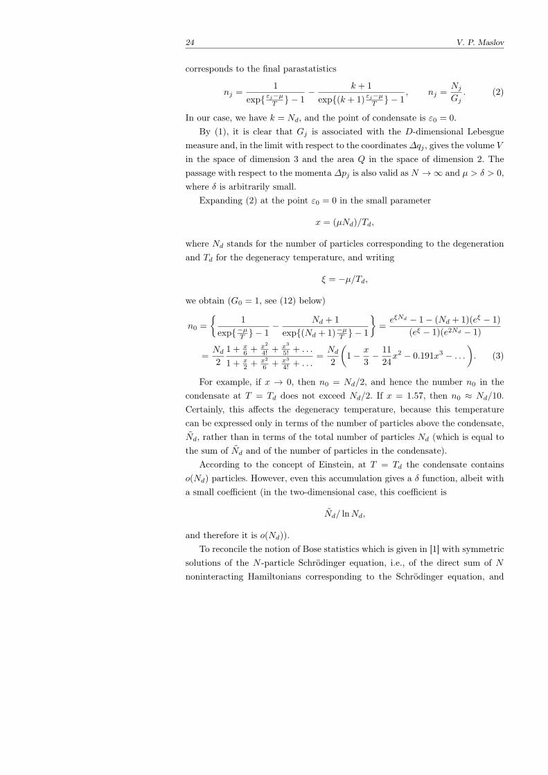
ber of particles and for energy. The number of states Gj is determined by theformula which mathematicians call the “Weyl relation;” it is described in detailin [2] in the “semiclassical case” in the section “Several degrees of freedom.” The2D-dimensional phase space is partitioned into a lattice, and the number Gj isdefined by the formula
Gi =∆pj∆qj(2πh)D
. (1)
The indeterminate Lagrange multipliers are expressed in terms of temperatureand chemical potential of the gas.
Further, in [1], following Einstein, a passage to the limit is carried out asN → ∞, which enables one to pass from sums to integrals. Then, in the section“Degenerate Bose gas,” a point is distinguished which corresponds to the energyequal to zero. This very point is the point of Bose condensate on which excessiveparticles whose number exceeds some value Nd ≫ 1 are accumulated at temper-atures below the so-called degeneracy temperature Td. The theoretical discoveryof this point anticipated a number of experiments that confirmed this fact notonly for liquid helium but also for a series of metals and even for hydrogen.
From a mathematical point of view, distinguishing a point in the integral isan incorrect operation if this point does not form a δ function. In particular,for the two-dimensional case, this incorrectness leads to a “theorem” formulatedin various textbooks and claiming that there is no Bose condensate in the two-dimensional case.
In this paper, we get rid of this mathematical incorrectness and show that,both in the two-dimensional and in the one-dimensional case, the Bose conden-sate exists if the point introduced above is well defined.
The main idea of the author in the proof of the occurrence of the Bosecondensate in the D-dimensional case is in a concordance between the chemicalpotential µ→ 0 and the number of particles N → ∞ when passing to the limit.
The phenomenon associated with the point of condensation holds only if thelimit as µ→ 0 depends on N → ∞.
If we accept Einstein’s remarkable discovery for the three-dimensional caseand justify it in a mathematically correct way, then the Bose condensate in thetwo-dimensional case is equally correct mathematically. We dwell on the two-dimensional case below in particular detail.
Thus, we consider the case in which N ≫ 1, but n is not equal to infin-ity. In the section “Ideal gas in the case of parastatistics” of the textbook byKvasnikov [3], there is a problem (whose number in the book is (33)) which
24 V. P. Maslov
corresponds to the final parastatistics
nj =1
exp εj−µT − 1− k + 1
exp(k + 1)εj−µT − 1
, nj =NjGj
. (2)
In our case, we have k = Nd, and the point of condensate is ε0 = 0.By (1), it is clear that Gj is associated with the D-dimensional Lebesgue
measure and, in the limit with respect to the coordinates∆qj , gives the volume Vin the space of dimension 3 and the area Q in the space of dimension 2. Thepassage with respect to the momenta ∆pj is also valid as N → ∞ and µ > δ > 0,where δ is arbitrarily small.
Expanding (2) at the point ε0 = 0 in the small parameter
x = (µNd)/Td,
where Nd stands for the number of particles corresponding to the degenerationand Td for the degeneracy temperature, and writing
ξ = −µ/Td,
we obtain (G0 = 1, see (12) below)
n0 =
1
exp−µT − 1
− Nd + 1
exp(Nd + 1)−µT − 1
=eξNd − 1− (Nd + 1)(eξ − 1)
(eξ − 1)(e2Nd − 1)
=Nd2
1 + x6 + x2
4! +x3
5! + . . .
1 + x2 + x2
6 + x3
4! + . . .=Nd2
(1− x
3− 11
24x2 − 0.191x3 − . . .
). (3)
For example, if x → 0, then n0 = Nd/2, and hence the number n0 in thecondensate at T = Td does not exceed Nd/2. If x = 1.57, then n0 ≈ Nd/10.Certainly, this affects the degeneracy temperature, because this temperaturecan be expressed only in terms of the number of particles above the condensate,Nd, rather than in terms of the total number of particles Nd (which is equal tothe sum of Nd and of the number of particles in the condensate).
According to the concept of Einstein, at T = Td the condensate containso(Nd) particles. However, even this accumulation gives a δ function, albeit witha small coefficient (in the two-dimensional case, this coefficient is
Nd/ lnNd,
and therefore it is o(Nd)).To reconcile the notion of Bose statistics which is given in [1] with symmetric
solutions of the N -particle Schrodinger equation, i.e., of the direct sum of Nnoninteracting Hamiltonians corresponding to the Schrodinger equation, and
Bose Condensate in the D-Dimensional Case 25
the symmetric solutions of their spectrum, it is more appropriate to assign tothe cells the multiplicities of the spectrum of the Schrodinger equation in theway described in [4].
Consider the nonrelativistic case in which the Hamiltonian H is equal to
p2/(2m),
where p stands for the momentum.The comparison of Gi with the multiplicities of the spectrum of the
Schrodinger equation gives a correspondence between the eigenfunctions of theN -partial Schrodinger equation that are symmetric with respect to the permu-tations of particles and the combinatorial calculations of the Bose statistics thatare presented in [1].
A single-particle ψ-function satisfies the free Schrodinger equation with theDirichlet conditions on the vessel walls. According to the classical Courant for-mula,
λj ∼2h2
m
(πD/2Γ (D/2 + 1)
V
)2/D
j2/D as j → ∞, (4)
where D stands for the dimension of the space, because the spectral density hasthe asymptotic behavior
ρ(λ) =V mD/2λD/2
Γ (D/2 + 1)(2π)D/2hD(1 + o(1)) as λ→ ∞. (5)
The asymptotics (4) is a natural generalization of this formula.Using this very correspondence, we establish a relationship between the Bose–
Einstein combinatorics [1], the definition of the N -particle Schrodinger equation,and the multiplicity of the spectrum of the single-particle Schrodinger equation.
The spectrum of the single-particle Schrodinger equation, provided that theinteraction potential is not taken into account, coincides, up to a factor, with thespectrum of the Laplace operator. Consider its spectrum for the closed interval,for the square, and for the D-dimensional cube with zero boundary conditions.This spectrum obviously consists of the sum of one-dimensional spectra.
On the line we mark the points i = 0, 1, 2, . . . and on the coordinate axes x, yof the plane we mark the points with x = i = 0, 1, 2, . . . and y = j = 0, 1, 2, . . . .To this set of points (i, j) we assign the points on the line that are positiveintegers, l = 1, 2, . . . .
To every point we assign a pair of points, i and j, by the rule i+ j = l. Thenumber of these points is nl = l + 1. This is the two-dimensional case.
26 V. P. Maslov
Consider the 3-dimensional case. On the axis z we set k = 0, 1, 2, . . . , i.e., let
i+ j + k = l
In this case, the number of points nl is equal to
nl =(l + 1)(l + 2)
2.
It can readily be seen, for the D-dimensional case, that the sequence ofmultiplicities for the number of variants
i =
D∑k=1
mk,
where mk are arbitrary positive integers, is of the form
qi(D) =(i+D − 2)!
(i− 1)!(D − 1)!, for D = 2, qi(2) = i, (6)
∞∑i=1
Ni = N, ε
∞∑i=1
qi(D)Ni = E. (7)
The following problem in number theory corresponds to the three-dimensional case D = 3 (cf. [1]):
∞∑i=1
Ni = N, ε
∞∑i=1
(i+ 2)!
i!6Ni = E,
E
ε=M. (8)
Write M = Ed/ε1, where ε1 stands for the coefficient in formula (4) for j = 1.Let us find Ed,
Ed =
∫ ∞
0
|p|22m dε
e|p|22m /Td − 1
, (9)
where
dε =|p|2
2m
dp1 . . . dpD dVD(2πh)D
. (10)
Whence we obtain the coefficient α in the formula,
Ed = αT 2+γd ζ(1 +D/2)Γ (1 +D/2). (11)
To begin the summation in (7) at the zero index (beginning with the zeroenergy), it is necessary to rewrite the sums (7) in the form
∞∑i=0
Ni = N, ε∞∑i=0
(qi(D)− 1)Ni = E − εN. (12)
Bose Condensate in the D-Dimensional Case 27
The relationship between the degeneracy temperature and the number Nd ofparticles above the condensate for µ > δ > 0 (where δ is arbitrarily small) canbe found for D > 2 in the standard way.
Thus, we have established a relationship between Gi in formula (1) (which iscombinatorially statistical) and the multiplicity of the spectrum for the single-particle Schrodinger equation, i.e., between the statistical [1] and quantum-mechanical definitions of Bose particles.
For D = 2, the general problem reduces to a number theory problem.Consider the two-dimensional case in more detail. There is an Erdos’ theorem
for a system of two Diophantine equations,∞∑i=1
Ni = N,
∞∑i=1
iNi =M. (13)
The maximum number of solutions of this system is achieved if the followingrelation is satisfied:
Nd = c−1M1/2d log Md + aM
1/2d + o(M
1/2d ), c = π
√2/3, (14)
and if the coefficient a is defined by the formula
c/2 = e−ca/2.
The decomposition of Md into one summand gives only one version. Thedecomposition Md into Md summands also provides only one version (namely,the sum of ones). Therefore, somewhere in the interval must be at least onemaximum of the variants. Erdos had evaluated it (14) (see [7]).
If the number N increases and M is preserved in the problem (13), then thenumber of solutions decreases. If the sums (13) are counted from zero ratherthan from one, i.e., if we set
∞∑i=0
iNi = (M −N),∞∑i=0
Ni = N, (15)
then the number of solutions does not decrease and remains constant.I’ll try to explain this effect. The Erdos–Lehner problem [5] is to decompose
Md into N ≤ Nd summands. Let us expand the number 5 into two summands.We obtain 3 + 2 = 4+ 1. The total number is 2 versions (this problem is knownas “partitio numerorum”). If we include 0 to the possible summands, we obtainthree versions: 5+0 = 3+2 = 4+1. Thus, the inclusion of zero makes it possibleto say that we expand a number into k ≤ n (positive integer) summands. Indeed,the expansion of the number 5 into three summands includes all the previous
28 V. P. Maslov
versions, namely, 5+0+0, 3+2+0, and 4+1+0, and adds new versions, whichdo not include zero.
In this case, the maximum number of versions for the decomposition of thenumber 5 into N summands (there are two versions) is achieved at N = 2 andN = 3 (the two values for the maximum number of versions for N above thecondensate).
In this case, the maximum does not change drastically [5]; however, the num-ber of versions is not changed, namely, the zeros, i.e., the Bose condensate, makeit possible that the maximum remains constant, and the entropy never decreases;after reaching the maximum, it becomes constant. This remarkable property ofthe entropy enables us to construct an unrestricted probability theory in thegeneral case [8].
Let us turn to a physical definition.Note first that, without changing the accuracy of the quantity whose loga-
rithm is evaluated, we can replace logMd by
(1/2) log(Nd/Q).
Then √Md =
2Nd/Q
c−1 log(Nd/Q) + a+ o
(NdQ
). (16)
In our case, Nd/Q corresponds to the number of particles above the condensate.According to formula (11), in the two-dimensional case we must set γ = 0
and find the coefficient α. Then formula (16) gives us a relationship between Ndand Td due to the fact that the number of particles in the condensate is o(Nd).
For details concerning the Bose condensate in the one-dimensional case, see[11], [12], and [13].
In fact, we have proved that there is a gap between µ > δ > 0 and µ = 0.In the one-dimensional case, this gap in the spectrum is much wider than thatin the two- and three-dimensional cases [11]. The consequences form a topic ofanother paper.
Remark 1 The author studied the relationship between the economy during acrisis and the Bose condensate, which corresponds to the bankruptcy [9]. Con-tinuing the correspondence principle proposed by Irving Fisher, an economistand a disciple of Gibbs (this principle is the “fundamental law of economics”),where the amount of money M corresponds to the number of particles N , theauthor suggested to compare the chemical potential to the negative value of thenominal interest rate, which corresponds to Friedman’s rule.
Bose Condensate in the D-Dimensional Case 29
The issue of money accompanied the fall of the nominal interest to 0.5%following this dependence in which the small parameter µ
TdNd became equal
to 12D , where D stands for the “number of degrees of freedom”, which can be
fractional (in our case, this number is the dimension) [8].In the paper [10] by E. M. Apfel’baum and V. S. Vorob’ev, taking into account
the de Boer parameter, the values Zc for helium were calculated experimentally,which, according to the author’s rule
Zc =ζ(D2 + 1)
ζ(D2 ),
enables one to determine the number D of degrees of freedom and to experimen-tally verify whether or not there is an empirical relation of this kind betweenµ and Td in thermodynamics. It was assumed that the Bose gas is not perfect(i.e., the Schrodinger equation with a potential is considered) and the value ofx = (µNd)/Td reflects the interaction between the particles, just as the Zenoline reflects the interaction between particles in classical thermodynamics [11].
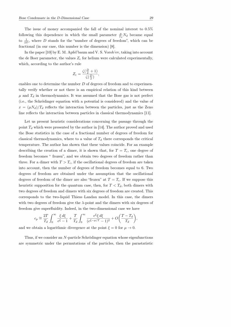
Let us present heuristic considerations concerning the passage through thepoint Td which were presented by the author in [14]. The author proved and usedthe Bose statistics in the case of a fractional number of degrees of freedom forclassical thermodynamics, where to a value of Td there corresponds the criticaltemperature. The author has shown that these values coincide. For an exampledescribing the creation of a dimer, it is shown that, for T = Tc, one degree offreedom becomes “ frozen”, and we obtain two degrees of freedom rather thanthree. For a dimer with T > Tc, if the oscillational degrees of freedom are takeninto account, then the number of degrees of freedom becomes equal to 6. Twodegrees of freedom are obtained under the assumption that the oscillationaldegrees of freedom of the dimer are also “frozen” at T = Tc. If we suppose thisheuristic supposition for the quantum case, then, for T < Td, both dimers withtwo degrees of freedom and dimers with six degrees of freedom are created. Thiscorresponds to the two-liquid Thiess–Landau model. In this case, the dimerswith two degrees of freedom give the λ-point and the dimers with six degrees offreedom give superfluidity. Indeed, in the two-dimensional case we have
cp ∼=2T
Td
∫ ∞
0
ξ dξ
eξ − 1+T
Td
∫ ∞
0
eξξ dξ
(eξ−µ/T − 1)2+O
(T − TdTd
),
and we obtain a logarithmic divergence at the point ξ = 0 for µ→ 0.
Thus, if we consider anN -particle Schrodinger equation whose eigenfunctionsare symmetric under the permutations of the particles, then the parastatistic
30 V. P. Maslov
correction leads to the fact that N/2 particles are in the condensate for T = Td
and N = Nd. For N > Nd, all the extra particles pass into the condensate state,which determines the dependence of the temperature T on N , and hence thedependence of N on the temperature for T < Td as well.
The case in which N is not so large as it is in statistical physics, i.e., theso-called mesoscopic state (see [14]), can also be of interest for us. In this case,let us use Fock’s idea for the Hartree equations, which lead to the Hartree–Fockequations.
Namely, we consider the single-particle equation of the mean field (a self-consistent field) and apply (to the resulting “dressed” potential) the procedureof transition to the N -partial Schrodinger equation with a dressed potential,just as we proceeded above for the operator h2
2m∆. Here we can consider twoways of investigation. The first way is the way used by Fock and which leads inthe semiclassical limit to the Thomas–Fermi equations for the dressed potential.Another way is to consider the Hartree temperature equations (see [15]) and toobtain the Thomas–Fermi temperature equations in the classical limit.
Since the quantity Td is small, it is easier to use the first way and to find the“dressed” potential.
Let V (q − q′) be a pairwise interaction potential such that∫|V (r)| dr <∞.
The dressed potential W (q) is given by the formula
W (q) = U(q) +
∫V (q − q′)|ψ(q′)|2 dq′,
where U(q) stands for the external potential and ψ(q′) for an eigenfunction of theSchrodinger equation which depends on the “dressed” potential and is thus anequation with a “unitary” nonlinearity. The expansion of the equation in powersof h can be found by the method of complex germ up to O(hk), where k is an anarbitrarily large number1 (see [23], where system (63) defines a complex germ;see also [24]– [30]). The superfluidity in nanotubes was confirmed experimentally.
The author thanks Professors G. I. Arkhipov, V. S. Vorob’ev, andV. N. Chubarikov for permanent discussions.
1 For U(q) ≡ 0, one obtains Bogolyubov’s famous equation [16]. The creation of dimers leadsto the ultrasecond quantization, i.e., to the operators of creation and annihilation of pairs. Thismakes it possible to satisfy the boundary conditions in a capillary ( [17]– [22]).
Bose Condensate in the D-Dimensional Case 31
References
1. L. D. Landau and E. M. Lifshits, Statistical Physics (Nauka, Moscow, 1964) [in Russian].2. L. D. Landau and E. M. Lifshits, Quantum Mechanics (Nauka, Moscow, 1976) [in Russian].3. I. A. Kvasnikov, Thermodynamics and Statistical Physics: Theory of Equilibrium Systems
(URSS, Moscow, 2002), Vol. 2 [in Russian].4. V. P. Maslov, “Mathematical Aspects of Weakly Nonideal Bose and Fermi Gases on a
Crystal Base”, Funktsional. Anal. i Prilozhen. 37 (2), 16–27 (2003) [Functional Anal.Appl. 37 (2), (2003)].
5. P. Erdos, J. Lehner, “The Distribution of the Number of Summands in the Partitions of aPositive Integer,” Duke Math. J. 8 (2), 335–345 (June 1941).
6. V. P. Maslov, “New Probability Theory Compatible with the New Conception of ModernThermodynamics: Economics and Crisis of Debts,” Russian Journal of Math. Physics 19(1), 63–100 (2012).
7. P. Erdos, “On some asymptotic formulas in the theory of partitions,” Bull. Amer. Math.Soc. 52, 185–188, (1946).
8. V.P.Maslov, “Unbounded Probability Theory Compatible with the Probability Theory ofNumbers,” Math. Notes, 91 (5) 603–609, (2012).
9. V. P. Maslov, “Theorems on the Debt Crisis and the Occurrence of Inflation,” Math. Notes,85 (1) 146–150, (2009).
10. E. M. Apfelbaum, V. S. Vorob’ev, “Correspondence between the Critical and the Zeno-LineParameters for Classical and Quantum Liquids,” J. Phys. Chem. B, 113 (11), 3521–3526(2009).
11. V. P. Maslov, ”Mathematical conception of “phenomenological” equilibrium thermodynam-ics”, Russ. J. Math. Phys. 18 (4), 363–370 (2011).
12. V. P. Maslov, ”Demonstrativeness in Mathematics and Physics,”, Russ. J. Math. Phys. 19(2), 163–175 (2012).
13. V.P.Maslov, “Binodal for the New Ideal Gas and the Ideal Liquid,” Math. Notes, 91 (6)893–894, (2012).
14. V. P. Maslov, ”Hypothetic λ-Point for Noble Gases,” Russ. J. Math. Phys. 17 (4), 400–413(2010).
15. V. P. Maslov, Complex Markov Chains and the Feynman Path Integral for NonlinearEquations (Nauka, Moscow, 1976) [in Russian].
16. N. N. Bogolyubov, On the Theory of Superfluidity, in Selected Works (Naukova Dumka,Kiev, 1970), Vol. 2 [in Russian].
17. V. P. Maslov, “On the dependence of the criterion for superfluidity from the radius of thecapillary,” Teoret. Mat. Fiz. 143 (3), 307–327 (2005) [Theoret. and Math. Phys. 143 (3),741–759 (2005)].
18. V. P. Maslov, “Resonance between one-particle (Bogoliubov) and two-particle series in asuperfluid liquid in a capillary,” Russ. J. Math. Phys. 12 (3), 369–379 (2005).
19. V. P. Maslov, “On the superfluidity of the classical fluid in a nanotube for even and oddnumbers of neutrons in a molecule,” Teoret. Mat. Fiz. 153 (3), 388–408 (2007) [Theoret.and Math. Phys. 153 (3), 1677–1696 (2007)].
20. V. P. Maslov, “On the superfluidity of classical liquid in nanotubes. I. Case of even numberof neutrons,” Russian J. Math. Phys. 14 (3), 304–318 (2007).
21. V. P. Maslov, “On the superfluidity of classical liquid in nanotubes. II. Case of odd numberof neutrons,” Russian J. Math. Phys. 14 (4), 401–412 (2007).
22. V. P. Maslov, “On the Superfluidity of Classical Liquid in Nanotubes. III,” Russian J.Math. Phys. 15 (1), 61–65 (2008).
23. V. P. Maslov, “Quasi-particles associated with Lagrangian manifolds corresponding tosemiclassical self-consistent fields. III,” Russ. J. Math. Phys. 3 (2), 271–276 (1995).
24. V. P. Maslov and O. Yu. Shvedov, The Method of Complex Germ. (URSS, Moscow,2000)[in Russian].
25. V. P. Maslov, The Complex WKB Method in Nonlinear Equations (Nauka, Moscow, 1977)[in Russian].
26. V. P. Maslov, The Complex WKB Method for Nonlinear Equations I (Birkhauser Verlag,Basel–Boston–Berlin, 1994).
27. V. P. Maslov, “On an Integral Equation of the Form u(x) = F (x) +∫G(x, ξ)u
(n−2)/2+ (ξ)dξ/
∫u(n−2)/2+ (ξ)dξ for n = 2 and n = 3”, Mat. Zametki 55 (3),
96–108 (1994) [Math. Notes 55 (3–4), 302–311 (1994)].
28. V. P. Maslov, “Spectral Series, Superfluidity, and High-Temperature Superconductivity”,58 (6), 933–936 (1995) [Math. Notes 58 (5–6), 1349–1352 (1995)].
29. V. P. Maslov and O. Yu. Shvedov, “The number of Bose-condensed particles in a weaklynonideal Bose gas,” Mat. Zametki 61 (5), 790–792 (1997) [Math. Notes, 61 (5), 661–664(1997)].
30. V. P. Maslov, “On an averaging method for the quantum many-body problem,” Funkt-sional. Anal. i Prilozhen. 33 (4), 50–64 (1999) [Funct. Anal. Appl. 33 (4), 280–291 (2000)].
The research was supported by the RFBR grants 12–01–00886-a and 11–01–12058_ofi_m and by the Joint grant of RFBR and CNRS 11-01-93106_a.
V. P. MaslovMoscow State University, Physics Department, Moscow, Russia.E-mail: [email protected]
Tropical and Idempotent Mathematics. Moscow, Russia, August 26–31, 2012
Fixed points of discrete convex monotone dynam-ical systems
Marianne Akian
Abstract Convex, order preserving maps of Rn include at the same time trop-ical or max-plus linear maps, and affine order-preserving maps of Rn. In theseparticular cases, the set of fixed points or additive eigenvectors and the con-vergence of the orbits are characterized respectively by the max-plus spectraltheorem and the Perron-Frobenius theorem. We shall give a survey of the char-acterizations that have been obtained for general convex, order preserving mapsof Rn. We shall also discuss the possible extension to the setting of stationarysolutions of Hamilton-Jacobi-Bellman equations.
This talk covers joint works with Stephane Gaubert, Benoıt David, and BasLemmens.
1 Convex, order-preserving maps as dynamic programmingoperators of stochastic control problems
A map f from Rn to itself is order-preserving if it preserves the partial order ofRn, that is f(v) ≤ f(v′) for all v, v′ ∈ Rn such that v ≤ v′, where v ≤ v′ meansvi ≤ v′i for all i = 1, . . . , n. It is convex if all its coordinates fi : Rn → R areconvex functions. It is additively homogeneous if it commutes with the additionof a constant vector f(λ+ v) = λ+ f(v) for all v ∈ Rn and λ ∈ R, where we usethe notation λ + v for the vector with entries (λ + v)i = λ + vi. It is additively
34 M. Akian
sub-homogeneous if f(λ + v) ≤ λ + f(v) for all v ∈ Rn and λ ≥ 0. An order-preserving additively sub-homogeneous map of Rn is necessarily nonexpansivefor the sup-norm.
Moreover, it can be put in the form
f(v)i := maxa∈Ai
n∑j=1
P(a)ij vj + r
(a)i
∀i ∈ [n], (1)
where [n] := 1, . . . , n, and for all i, j ∈ [n], a ∈ Ai, Ai is a subset of Rn,r(a)i ∈ R and P
(a)ij ≥ 0 with
∑nj=1 P
(a)ij ≤ 1. Then, f can be interpreted as the
dynamic programming operator of a stochastic control problem with state space[n], and set of possible actions Ai in state i ∈ [n], where r(a)i is the additivereward at each time when the process is in state i and applies the action a ∈ Ai,and P (a)
ij is the transition probability of the process from state i to state j, whenapplying the action a ∈ Ai, multiplied by some discount factor (which is ≤ 1)depending on i and a. Hence, when f is contracting, its fixed point is the valuefunction of an infinite horizon stochastic control problem, and the fixed pointiteration associated to f coincides with the value iteration of this problem. Whenf is additively homogeneous, the nonlinear additive eigenvalue of f , meaning aconstant ρ ∈ R such that there exists v ∈ Rn satisfying f(v) = ρ + v, is thevalue of the an ergodic stochastic control problem. These properties motivatethe study of fixed points, additive eigenvalue and eigenvectors, and convergenceof the orbits.
When f is not necessarily sub-homogeneous but still sends Rn to itself, itcan still be put in the form (1) for some P (a)
ij ≥ 0. Then, f can be interpreted asthe dynamic programming operator of a stochastic control problem, where nowdiscount factors may be greater than 1, or equivalently discount rates may begreater than 0. Such a problem arises for instance in sustainable development,and in portfolio management.
2 A convex spectral theorem
Important particular cases of (1) include the max-plus linear maps which cor-respond to deterministic control problems, and affine maps which correspondto stochastic problems with no action or control. In these particular cases, theset of fixed points or additive eigenvectors and the convergence of the orbits arecharacterized respectively by the max-plus spectral theorem and the (reducible)Perron-Frobenius theorem. Inspired by these characterizations, the following re-sult was shown in [2]. (The case when f is piecewise affine, or when the sets
Fixed points of discrete convex monotone dynamical systems 35
Ai are finite, was already treated in works by Schweitzer, Federgruen (77,78),Romanovski (73), and Lanery (67) using different techniques of proof.)
Theorem 1 (Convex spectral theorem [2]) Let f be order-preserving, addi-tively homogeneous and convex, and assume E(f) = ∅. Let C be the set of nodesof Gc(f) and r : Rn → RC , x 7→ xC = (xi)i∈C . Then
– r is an order-preserving and additively homogenous isomorphism and thus asup-norm isometry from E(f) to its image Ec(f).
– Ec(f) is an inf-subsemilattice of (RC ,≤) and is convex. Its dimension is atmost the number of strongly connected components of Gc(f), with equalitywhen f is piecewise affine.
– Let c = c(Gc(f)), then for all v ∈ Rn, fkc(v)− kcλ has a limit when k → ∞.
Let us explain the notations used in this theorem. Since f is nonexpansive, aneigenvalue λ is unique if it exists, then we denote by E(f) = v ∈ Rn | λ+ v =
f(v) the set of corresponding additive eigenvectors. Since f is convex, considerthe subdifferential of f at v defined by:
∂f(v) = M ∈ Rn×n | f(w)− f(v) ≥M(w − v) ∀w ∈ Rn.
Then ∂f(v) is rectangular: ∂f(v) = ∂f1(v)× · · · × ∂fn(v), where matrices M ∈Rn×n are identified to the n-uple of their rows (M1, . . . ,Mn). Moreover, ∂f(v)is non-empty, convex, compact, and included in the set Snn of n × n Markovmatrices. For any rectangular subset P of Snn, we denote Gc(P) :=
∪P∈P Gc(P ),
where Gc(P ) is the restriction of the directed graph G(P ) of the Markov matrixP to the set of recurrent (or equivalently final) nodes of P . When f has aneigenvector, the graph Gc(∂f(v)) is independent of the choice of v ∈ E(f) [2],which allows us to denote it by Gc(f). Then, c(Gc(f)) is the cyclicity of thisgraph, where the cyclicity of a strongly connected graph is the gcd of the lengthsof its cycles, and the cyclicity of a general graph is the lcm of its stronglyconnected components.
After an easy transformation [2], one can also obtain from Theorem 1 acharacterization of the set of fixed points and orbits of an order-preserving,additively sub-homogeneous and convex map f from Rn to itself. In that case,recurrent nodes of a sub-stochastic matrix P are the nodes belonging to a finalclass which has row sums equal to 1, then the critical graph of f may be empty,in which case the fixed point is unique.
In [3], we generalized the sub-homogeneous version of Theorem 1 to the caseof maps f that are not necessarily nonexpansive, by replacing the set of fixed
36 M. Akian
points of f by those satisfying a certain stability property, as follows. Namely, letD be an open and convex subset of Rn and f be an order-preserving and convexselfmap of D. Then, now ∂f(v) is still included in the set Pnn of n× n matriceswith nonnegative entries, but it may contain non substochastic matrices. We saythat a fixed point v of f is tangentially stable (t-stable) if all the orbits of f ′vare bounded (or equivalently bounded from above), where f ′v is the directionalderivative of f at v:
f ′v(w) := limt→0+
f(v + tw)− f(v)
t= supP∈∂f(v)
Pw ∀w ∈ Rn .
This implies (but is not equivalent to) the property that all P ∈ ∂f(v) arestable matrices. Moreover, if v is Lyapounov stable then v is t-stable, but thereverse implication fails. We denote by Et(f) the set of tangentially stable fixedpoints of f . For any rectangular subset P of Pnn, composed of stable matrices,we denote Gc(P) :=
∪P∈P Gc(P ), where Gc(P ) is the restriction of G(P ) to the
union of classes C of P such that ρ(PCC) = 1. When Et(f) = ∅, then Gc(∂f(v))is independent of the t-stable fixed point v of f , which allows us to denote itGc(f).
Theorem 2 ( [3]) Let D be an open, convex and downward subset of Rn, andf : D → D be order-preserving and convex. Assume Et(f) = ∅. Let C be the setof nodes of Gc(f) and r : Rn → RC , x 7→ xC = (xi)i∈C . Then
– r is an order-preserving isomorphism from Et(f) to its image Ect (f).– Ect (f) is an inf-subsemilattice of (RC ,≤) and is convex. Its dimension is at
most the number of strongly connected components of Gc(f).– Let c = c(Gc(f)), then the period of each t-stable periodic point of f dividesc.
We also proved a global convergence result, when D = Rn. For a convexselfmap f of Rn, we denote by f its recession map:
f(x) = limλ→∞
1
λf(λx) = sup
y∈Rn
f(y + x)− f(y), x ∈ Rn.
Theorem 3 ( [3]) If f has all its orbits bounded from above, then f is non-expansive with respect to some polyhedral norm.
Moreover, if f has a fixed point, then every orbit of f converges to a Lyapunovstable periodic orbit of f whose period divides c = c(Gc(f)).
3 Stationary solutions of Hamilton-Jacobi-Bellman equations
Fixed points equations of maps f of the form (1) can also be obtained as dis-cretizations of Hamilton-Jacobi-Bellman partial differential equations associatedto optimal control problems of diffusions, when using a monotone scheme. Thissuggests that similar results may hold for Hamilton-Jacobi-Bellman equations.The study of first order equations, corresponding to deterministic control prob-lems and for which the semigroup is max-plus linear by the Maslov superpositionprinciple, is the object of the so called Weak KAM theory, see in particular theresults of Fathi and Siconolfi (05) which give characterizations of stationary so-lutions of Hamilton-Jacobi equations similar to the ones of max-plus spectraltheorem. In [1], we considered a particular stochastic control problem in the n-dimensional torus, and proved a similar characterization as in Theorem 1, whichgeneralize similar results obtained in the deterministic case by Rouy and Tourin(92), and Kolokoltsov and Maslov (97).One may thus ask if the same can occurfor the possible negative discount case.
References
1. M. Akian, B. David, and S. Gaubert. Un theoreme de representation des solutions deviscosite d’une equation d’Hamilton-Jacobi-Bellman ergodique degeneree sur le tore. C. R.Acad. Sci. Paris, Ser. I, 346:1149–1154, 2008.
2. M. Akian and S. Gaubert. Spectral theorem for convex monotone homogeneous maps, andergodic control. Nonlinear Analysis. Theory, Methods & Applications, 52(2):637–679, 2003.See also ttp://www.arXiv.org/abs/mat/0110108.
3. M. Akian, S. Gaubert, and B. Lemmens. Stability and convergence in discrete convexmonotone dynamical systems. Journal of Fixed Point Theory and Applications, 9:295–325,2011. 10.1007/s11784-011-0052-1.
The work was partially supported by the joint RFBR-CNRS grant 11–01–93106-a.
Marianne AkianINRIA, Saclay–Ile-de-France, and CMAP, Ecole Polytechnique, Route deSaclay, 91128 Palaiseau Cedex, France.E-mail: [email protected]
Tropical and Idempotent Mathematics. Moscow, Russia, August 26–31, 2012
Gagliardo type Inequality: an idempotent point ofview
Antonio AvantaggiatiPaola Loreti
Abstract We discuss a result obtained in collaboration with A. Avantaggiati.
In [2] we established a Gagliardo inequality in Gaussian space.The original result, established by Gagliardo in [3], holds for Lebesgue measureon Lipschitzian bounded sets. In [2] we adapted the original proof containedin [3] to Gaussian measure.Let us recall briefly the result. Denote by RN = R1 × . . .RN with Rj = R asj = 1, . . . N.
For any fixed k with 1 ≤ k ≤ N , we denote by σ a k-tuple of indices from theset 1, . . . , N , i.e., σ = (i1, . . . , ik) with i1 < i2 < · · · < ik, and by σ′ the (N − k)-tuple of the indices different from i1, i2, . . . , ik (in other words, complementaryto i1, i2, . . . , ik). Also x will be the N -vector x = (x1, x2, . . . , xN ), xσ will be thesubvector (xi1 , xi2 , . . . , xik), and σ′ = (i′1, . . . , i
′N−k).
Then Rσ = Ri1 × . . .Rik and RN = Rσ×Rσ′. A function f defined in RN is also
written as f(x) = f(x1, x2, . . . , xN ) = f(xσ, xσ′), and also, if g is defined in Rσ,gσ = g(xσ). Similarly, the Gaussian measure is dγ = (2π)−
N2 exp(−1
2 |x|2)dx =∏N
j=1(2π)− 1
2 exp(− 12 |xj |
2)dx, and dγσ =∏j∈σ(2π)
− 12 exp(−1
2 |xj |2)dx, with
dγ = dγσdγσ′ and we have∫Rσ dγσ(xσ) = 1. By Lp(RN , dγ) we denote the
Lp space with respect to dγ.We denote by S the set of all k-tuples of indices from 1, . . . , N . The number ofelements in S is
(Nk
). The result obtained in [2] is the following
1 Gagliardo type inequality
Theorem 1 Given(Nk
)functions Fσ(xσ) with σ ∈ S, and λ =
(N−1k−1
)satisfying
Fσ ∈ Lλ(Rσ, dγσ). we define
F (x) =∏σ∈S
Fσ(xσ).
Then F ∈ L1(RN , dγ) and(∫RN
|F (x)|dγ)λ
≤∏σ∈S
∫Rσ
|Fσ(xσ)|λdγσ,
In [2] we established a connection between the well-known Fubini theoremand its analogue in idempotent analysis, giving a proof which shows how topass from usual setting to the idempotent setting, and it is based on Gagliardoinequality in Gaussian space.
We discuss this result, related questions and further developments.
References
1. R. A. Adams, Sobolev Spaces, Academic Press (1975).2. A. Avantaggiati, P. Loreti, Gagliardo type Inequality and Application, Percorsi incrociati
(in ricordo di Vittorio Cafagna) Rubbettino Editore 2010.3. E. Gagliardo, Proprieta di alcune classi di funzioni in piu variabili, Ricerche Mat. 7 1958
102–137.4. G. L. Litvinov and V. P. Maslov, Idempotent mathematics: correspondence principle and
applications, Russian Mathematical Surveys 51 (1996), no. 6.
Antonio AvantaggiatiDipartimento di Scienze di Base e Applicate per l’Ingegneria. Sapienza Univer-sita di Roma, Italy.E-mail: [email protected]
Paola LoretiDipartimento di Scienze di Base e Applicate per l’Ingegneria. Sapienza Univer-sita di Roma, Italy.E-mail: [email protected]
Tropical and Idempotent Mathematics. Moscow, Russia, August 26–31, 2012
The Galileo invariance of diffusion scattering ofwaves in the phase space
E. M. Beniaminov
Abstract In the paper, we discuss the studies of mathematical models ofdiffusion scattering of waves in the phase space, and relation of these modelswith quantum mechanics. In the previous works it is shown that in these modelsof classical scattering process of waves, the quantum mechanical descriptionarises as the asymptotics after a small time. In the paper it is shown thatthe proposed models of diffusion scattering of waves possess the property ofgauge invariance. This implies that they are described similarly in all inertialcoordinate systems, i. e., they are invariant under the Galileo transformations.
1 Introduction
In the present paper we discuss the research on construction of models of diffusionscattering of waves in phase space. I have been studying this subject duringlast years [1–4]. In these models the quantum description of processes arises asan approximate one, asymptotical for large values of certain coefficients of themodel.
In the papers mentioned above one makes an attempt to construct a modelof quantum observables on the base of wave functions on the phase space. Notethat in quantum mechanics, the wave function depends either only on coordi-nates or only on momenta, while in the present approach one considers wave
The Galileo Invariance of Diffusion Scattering of Waves in the Phase Space 41
functions depending both on coordinates and on momenta. This model is basedalso on the following observation. In quantum mechanics, the phase of the wavefunction of a particle (the natural hidden parameter) changes in time even forstationary states with very high velocity (if one takes into account the station-ary energy). This velocity is such that a transfer of the particle with even small(non-relativistic) velocities can cause considerable changes in the phase of wavefunction because of the relativistic effect of more slow inner processes of a movingparticle. Already taking into account this effect leads to non-commutativity ofthe action of coordinate and momentum shifts on the wave function. Note onceagain that in the proposed model one considers wave functions on the phase(and not configuration) space, and one assumes that the particle is in a diffusionprocess causing random shifts of the wave both by coordinates and by momenta.It is shown that the classical model of scattering of the wave, taking into accountthe assumptions described above, yields to arising quantum effects.
In the paper it is shown that the proposed models of diffusion scatteringof waves possess the property of gauge invariance. This implies that they aredescribed similarly in all inertial coordinate systems, i. e., they are invariantunder the Galileo transformations.
2 The results obtained earlier
In the paper [4] we consider the Kramers equation [5], [6] of the form
∂f
∂t=
n∑j=1
(∂V
∂xj
∂f
∂pj− pjm
∂f
∂xj
)+ γ
n∑j=1
∂
∂pj
(pjf + kTm
∂f
∂pj
), (1)
where f(x, p, t) is the probability density of a particle in the phase space at themoment of time t; m is the mass of the particle; V (x) is the potential functionof external forces acting on the particle; γ = β/m is the resistance coefficient ofthe medium in which the particle moves, per unit of its mass; k is the Boltzmannconstant; T is the temperature of the medium.
Then we consider the modified Kramers equation for the wave functionφ(x, p, t) of the form
∂φ
∂t= Aφ+ γBφ, (2)
where Aφ =n∑j=1
(∂V
∂xj
∂φ
∂pj− pjm
∂φ
∂xj
)− i
~
(mc2 + V −
n∑j=1
p2j2m
)φ (3)
and Bφ =n∑j=1
∂
∂pj
((pj + i~
∂
∂xj
)φ+ kTm
∂φ
∂pj
).
42 E. M. Beniaminov
Equation (2) is obtained from the Kramers equation (1) by adding to the righthand side of the summand of the form −i/~(mc2 + V − p2/(2m))φ, and thereplacement, in the diffusion operator, of multiplication of the function φ by pjby the action of the operator (pj + i~∂/∂xj) on the function φ.
Adding the summand −i/~(mc2 + V − p2/(2m))φ is related with the addi-tional physical requirement that the wave function at the point (x, p) oscillatesharmonically with frequency 1/~(mc2 + V − p2/(2m)) in time.
The requirement of harmonic oscillating of the wave function φ at the point(x, p) with the large frequency 1/~(mc2 + V − p2/(2m)), in the case when mc2
is much greater than V, leads to the fact that the shift of the wave function withrespect to the coordinate xj with conservation of the proper time at the point(x, p) yields the phase shift in the oscillation of the function φ. And the operatorof infinitely small shift ∂/∂xj is changed by the operator ∂/∂xj − ipj/~. (Fora more detailed explanation, see [3].) Respectively, if we multiply this operatorby i~, then we obtain the operator pj + i~∂/∂xj , used in the modified diffusionoperator B.
For equation (2), in [4] we obtain results similar to that of the paper [3].It is shown that also in this case, the process described by equation (2), forlarge γ = β/m passes several stages. During the first rapid stage, the wavefunction goes to a “stationary” state. At the second, slow stage, the wave functionevolves in the subspace of “stationary” states subject to the Schrodinger equation.Besides that, it is shown that at the third stage, the dissipation of the processleads to decoherence of the wave function, and any superposition of states comesto one of eigenstates of the Hamilton operator.
In the paper [4], it is shown also that if, on the contrary, the medium resis-tance per unit of mass of the particle γ = β/m is small, and in equation (2) onecan neglect the summand with the factor γ, then in the considered model, thedensity of the probability distribution ρ = |φ|2 satisfies the standard Liouvilleequation
∂ρ
∂t=
n∑j=1
(∂V
∂xj
∂ρ
∂pj− pjm
∂ρ
∂xj
), (4)
as in classical statistical mechanics.
3 Gauge transformations
In this section we introduce and discuss the notion of gauge invariance for equa-tion (2).
The Galileo Invariance of Diffusion Scattering of Waves in the Phase Space 43
According to the approach exposed in [4], the density of probability distribu-tion ρ(x, p, t) of a quantum particle whose state at the moment of time t is givenby the wave function φ(x, p, t), is proportional to |φ|2 = φ(x, p, t)φ∗(x, p, t). Thisimplies that the replacement of a wave function φ by the wave function of theform exp(ig/~)φ, where g = g(x, p, t) is an arbitrary real valued function, doesnot change the density of the probability distribution ρ(x, p, t). Such a transformof wave function is usually called a gauge transform.
Let us look how equation (2) changes under this gauge transform. To thisend, let us write out equation (2) in a more general form. Let us write in it,instead of the differentiation operators ∂/∂pj of the function φ, the operatorDpj = ∂/∂pj + iBj/~, instead of the operators ∂/∂xj − ipj/~, the operator
Dxj = ∂/∂xj + iAj/~, and instead of the operator ∂/∂t + iH/~, where H =
mc2+p2/(2m)+V , let us write the operatorDx0 = ∂/∂t+iA0/~, where Aj , A0, Bj
are functions of x, p, and t for j = 1, ..., n. In these notations, equation (2) willtake the form
Dx0φ =
n∑j=1
(∂H
∂xjDpjφ− ∂H
∂pjDxj φ
)+ γ
n∑j=1
Dpj
(i~Dx
j φ+ kTmDpjφ). (5)
By a gauge transform of equation (5) we call the following transform of thefunction φ and the potentials Aj , A0, Bj , for j = 1, ..., n:
φ 7−→ φ′ = exp(− i
~g)φ; (6)
A0 7−→ A′0 = A0 +
∂g
∂t;
Aj 7−→ A′j = Aj +
∂g
∂xj, where j = 1, ..., n;
Bj 7−→ B′j = Bj +
∂g
∂pj, where j = 1, ..., n. (7)
It is not difficult to see that after the substitution (6) into equation (5), re-placement (7), and dividing both parts of the obtained equality by exp(−(i/~)g),the form of equation (5) will not change.
Geometrically, gauge transformation corresponds to transfer to another trivi-alization of a complex line bundle over the phase space, in which a form of linearconnection is chosen, defining parallel transport of the vectors of the bundlealong trajectories in the phase space.
In the particular case for equation (2), the potentials read
A0 = H(x, p) = E + V ; Aj = −pj ; Bj = 0 for j = 1, ..., n.
44 E. M. Beniaminov
Understanding the physical sense of the potentials in the general case forequation (5), requires separate investigation. For the Dirac equation, potentialsof gauge invariance are usually related with the potentials of electromagneticfield.
4 The Galileo invariance
In this section we study the change of equation (2) under the transfer to a co-ordinate system moving uniformly with respect to the initial coordinate system,with the velocity u. The diffusion equation (1) is not invariant with respect toGalileo transforms under transfer to new inertial coordinate system moving withconstant velocity u with respect to the old one.
The aim of this section is to study invariance of equation (2) for a free particle(V = 0) with respect to Galileo transforms, with gauge transforms of the wavefunction.
By definition of Galileo transforms, the new coordinate system is expressedthrough the old one by the following formulas:
t′ = t; x′ = x− ut; p′ = p−mu;
E′ =p′2
2m=
(p−mu)2
2m=
p2
2m− pu+
mu2
2= E − pu+
mu2
2. (8)
Respectively, the old coordinates are expressed through the new ones by thefollowing formulas:
t = t′; x = x′ + ut; p = p′ +mu;
E =p2
2m=
(p′ +mu)2
2m=p′2
2m+ p′u+
mu2
2= E′ + p′u+
mu2
2. (9)
Substituting these expressions into equation (2), with the use of relations (3)and (4), we obtain:
∂φ
∂t′−
n∑j=1
∂φ
∂x′juj =
n∑j=1
(∂V
∂x′j
∂φ
∂p′j−p′j +muj
m
(∂
∂x′j− i
p′j +muj
~
)φ
)
− i
~
(E′ + p′u+
mu2
2+ V
)φ
+γn∑j=1
∂
∂p′j
((p′j +muj + i~
∂
∂x′j
)φ+ kTm
∂φ
∂p′j
),
whence, after simple algebraic transformations, we obtain:
∂φ
∂t′=
n∑j=1
(∂V
∂x′j
∂φ
∂p′j−p′jm
(∂
∂x′j− i
p′j +muj
~
)φ
)
− i
~
(E′ − mu2
2+ V
)φ
+γn∑j=1
∂
∂p′j
((p′j +muj + i~
∂
∂x′j
)φ+ kTm
∂φ
∂p′j
).
If in the obtained equation one makes the substitution φ = exp((i/~)g)φ′,
where g = mux′ + mu2t′/2, then (after the gauge transform) we obtain theequation
∂φ′
∂t′=
n∑j=1
(∂V
∂x′j
∂φ′
∂p′j−p′jm
(∂
∂x′j− i
p′j~
)φ′)
− i
~(E′ + V )φ′
+γn∑j=1
∂
∂p′j
((p′j + i~
∂
∂x′j
)φ′ + kTm
∂φ′
∂p′j
),
which coincides with equation (2). Thus, we have proved the Galileo invarianceof equation (2).
References
1. Beniaminov, E.M.: A Method for Justification of the View of Observables in Quan-tum Mechanics and Probability Distributions in Phase Space. http://arxiv.org/abs/quant-ph/0106112 (2001)
2. Beniaminov, E.M.: Diffusion processes in phase spaces and quantum mechanics. DokladyMathematics (Proceedings of the Russian Academy of Sciences) 76, 771–774 (2007)
3. Beniaminov, E.M.: Quantization as asymptotics of a diffusion process in phasespace. Proc. Intern. Geom. Center 2(4), 7-50 (2009) (in Russian; English translation:http://arXiv.org/abs/0812.5116v1)
4. Beniaminov, E.M.: Quantum Mechanics as Asymptotics of Solutions of GeneralizedKramers Equation. Electronic Journal of Theoretical Physics (EJTP) 8, No. 25 195-210(2011)
5. Kramers, H. A.: Brownian motion in a field of force and the diffusion model of chemicalreactions. Physica. 7, 284-304. (1940)
6. Van Kampen, N.G.: Stochastic Processes in Physics and Chemistry. North Holland, Am-sterdam (1981)
E. M. BeniaminovRussian State University for the Humanities, Moscow, RussiaE-mail: [email protected]
Tropical and Idempotent Mathematics. Moscow, Russia, August 26–31, 2012
General transience bounds in tropical linear alge-bra via Nachtigall decomposition
Bernadette Charron-BostThomas Nowak
Abstract We present general transience bounds in tropical linear algebrabased on Nachtigall’s matrix decomposition. Our approach is also applicableto reducible matrices. The core technical novelty are general bounds on thetransient of the maximum of two eventually periodic sequences. Our proof isalgebraic in nature, in contrast to the existing purely graph-theoretic approaches.
1. Introduction
Tropical linear systems describe the behavior of transportation systems, manu-facturing plants, network synchronizers, as well as certain distributed algorithmsfor resource allocation and routing. It is known that the sequence of tropicalmatrix powers, and hence every linear system, becomes periodic after an initialtransient. In applications it is of interest to have upper bounds on the transient,to which we contribute with this work.
We use the Nachtigall decomposition [5] of square matrices in tropical algebrato show new transience bounds for sequences of matrix powers. The Nachtigalldecomposition is a representation of the sequence of matrix powers of a squarematrix as a maximum of a bounded number of sequences of bounded transientsand bounded periods. Transience bounds for the sequence of matrix powers havebeen given, amongst others, by Hartmann and Arguelles [4] and Charron-Bost et
General Transience Bounds via Nachtigall Decomposition 47
al. [1]. Their proofs are purely graph-theoretic. They consider the edge-weightedgraph described by the matrix as an adjacency matrix and argue about existenceof walks of certain weights. We, too, use this graph interpretation of a matrix intwo supplementary results (Lemma 2 and Lemma 6). However, the rest of ourproof is algebraic. Because our proof is based on the Nachtigall decomposition,which is also applicable to reducible matrices, so is our proof. To the best ofour knowledge, we are the first to give transience bounds for reducible matrices.An example by Even and Rajsbaum [3, Fig. 2] shows that our new bounds areasymptotically optimal.
2. Preliminaries
We consider the max-plus semiring on the set R = R ∪ −∞. That is, weconsider the addition (x, y) 7→ max(x, y) and the multiplication (x, y) 7→ x+ y.The semiring’s zero element is −∞ and its unit is 0. The matrix multiplication oftwo matrices A and B of compatible size satisfies (AB)i,j = maxk(Ai,k +Bk,j).
We call a sequence f : N → R eventually periodic if there exist numbers p,T , and ϱ such that:
∀n > T : f(n+ p) = f(n) + p · ϱ (1)
In this case we call p a period, T a transient, and ϱ a ratio of the sequence f . Itis easy to see that the ratio is unique and finite if the sequence is not eventuallyconstantly infinite. For every period p, there exists a unique minimal transient Tthat satisfies (1). The next fundamental lemma shows that these minimal tran-sients do, in fact, not depend on p:
Lemma 1 Let f : N → R be eventually periodic. Let p and p be periods of fwith respective minimal transients Tp and Tp. Then Tp = Tp.
We will henceforth call this unique minimal transient the transient of f . Also,we will call the minimal period the period of f .
Cohen et al. [2] established that the entrywise sequences of matrix powers An
of a square matrix are eventually periodic. More generally, we say that a sequenceof matrices is eventually periodic if every entrywise sequence is eventually peri-odic. Period and transience of a matrix sequence is a period and transience forall entrywise sequences.
The tropical convolution f ⊗ g of two sequences f and g is defined as
(f ⊗ g)(n) = maxn1+n2=n
(f(n1) + g(n2)
). (2)
48 B. Charron-Bost, T. Nowak
To a square matrix A naturally corresponds an edge-weighted digraph G(A).The weight p(W ) of a walk W in G(A) is the sum of the weights of its edges.The matrix powers of A satisfy the correspondence(
An)i,j
= maxp(W ) |W has length n and is from i to j
. (3)
3. Nachtigall Decomposition
Nachtigall [5] introduced a representation of the sequence of matrix powers ofan N ×N square matrix as the maximum of at most N matrix sequences whosetransients are at most 3N2. He showed that this representation can be computedefficiently. However, no results on the transient of the original matrix were ob-tained. The core of the representation is a decomposition of the original matrixinto components corresponding to cycles in the matrix’ digraph, The matrix se-quences are defined as convolutions corresponding to this decomposition. Thefollowing lemma shows the utility of maximum mean cycles for the decomposi-tion.
Lemma 2 ( [5, Lemma 3.2]) If A is an N × N matrix and k is a node ofa maximum mean cycle C in G(A), then both sequences
(An)i,k
and(An)k,i
are eventually periodic with period ℓ(C), ratio p(C)/ℓ(C), and transient at mostℓ(C) · (N − 1).
Given an N ×N matrix A and a set I ⊆ 1, . . . , N of indices, we define thedeletion of I in A as the matrix B whose entries satisfy Bi,j = −∞ if i ∈ I orj ∈ I, and Bi,j = Ai,j otherwise.
The following lemmas are used to prove the upper bound on the transient ofeach matrix sequence in the Nachtigall decomposition.
Lemma 3 Let f, g : N → R be eventually periodic with common period p, com-mon ratio ϱ, and respective transients Tf and Tg. Then the sequence max(f, g)
is eventually periodic with period p, ratio ϱ, and transient at most max(Tf , Tg).
Lemma 4 ( [5, Lemma 6.1]) Let f, g : N → R be eventually periodic withcommon period p, common ratio ϱ, and respective transients Tf and Tg. Thenthe convolution f ⊗ g is eventually periodic with period p, ratio ϱ, and transientat most Tf + Tg + p− 1.
We now state an improvement of Nachtigall’s theorem using essentially thesame arguments as the original version. The improvement lies in an upper boundof 2N2 −N on the sequences’ transients instead of 3N2.
General Transience Bounds via Nachtigall Decomposition 49
Theorem 1 (Nachtigall decomposition [5, Theorem 3.3]) Let A bean N × N matrix. Then there exist eventually periodic matrix sequencesA1(n), A2(n), . . . , AN (n) with periods at most N and transients at most 2N2−Nsuch that for all n:
An = max(A1(n), A2(n), . . . , AN (n)
)(4)
The proof proceeds by induction on N . The case N = 1 is trivial.
If G(A) does not contain a cycle, then (An)i,j = −∞ for all n > N , so thetransient of A is at most N and the theorem’s statement is trivially fulfilledwhen choosing all matrix sequences Am(n) equal to An.
We hence suppose that G(A) contains a cycle. By the definition of the matrixmultiplication, whenever n = n1 + n2, we have:
(An)i,j = maxk
((An1)i,k + (An2)k,j
)(5)
Let C be a maximum mean cycle in G(A). Denote by B the deletion of theset of C’s nodes in A. It follows from the definition of deletion and from thegraph interpretation (3) that
(An)i,j = max(maxk in C
((An1)i,k + (An2)k,j
), (Bn)i,j
). (6)
In particular, (6) continues to hold when forming the maximum over all n1and n2 such that n = n1 + n2. By writing Ai,j(n) = (An)i,j and recalling thedefinition (2) of convolution, we can hence write
(An)i,j = max(maxk in C
(Ai,k ⊗Ak,j
)(n) , (Bn)i,j
). (7)
Lemmas 2, 3, and 4 imply that the transient of the inner maximum in (7) isat most
2 · ℓ(C) · (N − 1) + ℓ(C)− 1 6 2N2 −N − 1 (8)
and its period is at most ℓ(C) 6 N . Choose the matrix sequence A1(n) equal tothis inner maximum, i.e., A1(n) = max
k in C
(Ai,k ⊗Ak,j
)(n).
By induction hypothesis, there exist matrix sequences A2(n),. . . ,AN (n)
with periods at most N and transients at most 2N2 − N such that Bn =
max(A2(n), . . . , AN (n)
). This then concludes the proof’s inductive step.
50 B. Charron-Bost, T. Nowak
4. Transience Bounds
Note that Theorem 1 does not imply that the transient of any sequence of matrixpowers is at most 2N2−N . The reason for this is that Lemma 3 is not applicableto the maximum in the Nachtigall decomposition because the involved sequencescan have different ratios.
The following lemma is our main technical novelty and provides a tool forbounding the transient of a maximum of two eventually periodic sequences iftheir ratios are not equal.
Lemma 5 Let f, g : N → R be eventually periodic with the same period p,respective ratios ϱf and ϱg, and respective transients Tf and Tg. Assume thatϱf > ϱg and that for all n > S we have g(n) = −∞ whenever f(n) = −∞. Thenthe sequence max(f, g) is eventually periodic with period p, ratio max(ϱf , ϱg),and transient at most
max(Tf , Tg, S) +Γ
|ϱf − ϱg|where
Γ = maxf(m)− g(m) | S 6 m < S + p , g(m) = −∞
.
In the rest of this section, we provide general transience bounds for sequencesof matrix powers. We do this by applying Lemma 5 entrywise to the maximumin (4). Evidently, given a Nachtigall decomposition (which is not unique), onecan use Lemma 5 to bound the transient of the matrix powers. In this section,we proceed to use the existence of a Nachtigall decomposition to prove generaltransience bounds independent of an explicit decomposition.
We first assume that the graph G(A) is strongly connected. In this case, allsequences (An)i,j are eventually periodic with ratio equal to the maximum cyclemean inG(A). For every pair (i, j) of indices, the ratio of the sequence
(Am(n)
)i,j
is greater or equal to that of(Am+1(n)
)i,j
. We want to apply Lemma 5 to everypair of (i) a sequence of maximum ratio and (ii) a sequence of another ratio.Afterwards, we apply Lemma 3 to the resulting maxima (which all have the sameratio). But to effectively apply Lemma 5, we have to bound its parameter S forevery pair.
We show that the parameter S is at most N(N + 1) with a graph-theoreticargument: The exploration penalty of graph G is the least integer ep such thatthere exists a closed walk of length n at every node in G for all multiples n ofG’s cyclicity2 that satisfy n > ep.
2 The cyclicity of a strongly connected graph is the greatest common divisor of its cyclelengths.
General Transience Bounds via Nachtigall Decomposition 51
Lemma 6 ( [1, Theorem 3]) The exploration penalty of a graph with N nodesis at most N(N − 1).
It is well-known that the difference of lengths of two walks from i to j in astrongly connected graph is always a multiple of the graph’s cyclicity. In eachstep of the Nachtigall recursion, there exists a path from i to j via a node kof C of length at most 2N . Hence Lemma 6 implies that if there exists any pathfrom i to j of length n > 2N + N(N − 1) = N(N + 1), then there exists alsoa path from i to j via k of length n. This shows that S can be chosen to be atmost N(N + 1).
A common period p of a pair of sequences is the least common multiple of thetwo periods. Because in the Nachtigall decomposition the periods are at most N ,there exists a common period less or equal to N(N − 1). Hence S + p can bebounded by 2N2.
We thus arrive at the following theorem bounding the transient of the se-quence of matrix powers. Denote by ∥A∥ the difference of the maximum and theminimum finite entry in matrix A.
Theorem 2 Let A be an N × N matrix such that G(A) is strongly connected.Denote by λ the maximum cycle mean in G(A) and λ′ the second largest cyclemean weight. Then the sequence of matrix powers An has transient at most
2N2 +∥A∥2N2
λ− λ′.
Hartmann and Arguelles [4, Theorem 10] arrived at a bound of ∥A∥2N2/(λ−λ0) on the transient, where λ0 is a parameter of the max-balanced graph of G(A).Their bound is always smaller than ours in Theorem 2. However, in the worstcase, both are asympotically in the same order of growth. Also, our technique isdifferent than that of Harmann and Arguelles, and can also be used to providesharper bounds if information on the Nachtigall decomposition is available.
Our technique is also applicable to the general case where G(A) is not nec-essarily strongly connected. In the general case, the ratio λi,j of the sequenceof entries (An)i,j is equal to the maximum mean of cycles reachable from i andfrom which j is reachable. Denote by λ′i,j the second largest mean of cycles reach-able from i and from which j is reachable. By analogous arguments, Theorem 2continues to hold in the general case if we replace the denominator λ − λ′ bymini,j(λi,j − λ′i,j).
References
1. Bernadette Charron-Bost, Matthias Fugger, and Thomas Nowak. On the transience of linearmax-plus dynamical systems. Under submission, 2011. arXiv:1111.4600v1 [cs.DM]
2. Guy Cohen, Didier Dubois, Jean-Pierre Quadrat, and Michel Viot. Analyse du comporte-ment periodique de systemes de production par la theorie des dioides. INRIA RR 191,1983.
3. Shimon Even and Sergio Rajsbaum. The use of a synchronizer yields maximum computationrate in distributed systems. Theory of Computing Systems 30(5):447–474, 1997.
4. Mark Hartmann and Cristina Arguelles. Transience bounds for long walks. Mathematics ofOperations Research 24(2):414–439, 1999.
5. Karl Nachtigall. Powers of matrices over an extremal algebra with applications to periodicgraphs. Mathematical Methods of Operations Research 46:87–102, 1997.
Bernadette Charron-BostEcole Polytechnique, Palaiseau, FranceE-mail: [email protected]
Thomas NowakEcole Polytechnique, Palaiseau, FranceEmail: [email protected]
Tropical and Idempotent Mathematics. Moscow, Russia, August 26–31, 2012
Planar flows and quadratic relationsover semirings
Vladimir I. DanilovAlexander V. KarzanovGleb A. Koshevoy
1 Introduction
In this work, acting in spirit of Lindstrom’s construction [7], we consider a wideclass of functions which take values in an arbitrary commutative semiring andare generated by flows (systems of paths) in a planar acyclic directed graph.Functions of this sort satisfy plenty of “stable” (or “universal”) quadratic rela-tions, extending well-known quadratic relations for minors of matrices (in par-ticular, Plucker’s and Dodgson’s ones) and their tropical analogues. We developa combinatorial method to completely characterize the set of such “stable” re-lations. In particular, applying this method to Gessel–Viennot’s model, one candescribe quadratic relations on Schur functions (related to semi-standard Youngtableaux). The full version of this work is to appear in J. Algebraic Combina-torics (DOI 10.1007/s10801-012-0344-6); see also Arxiv:1102.2578v2[math.CO].
We start with specifying terminology and notation, and with backgrounds.
1.1 Commutative semirings
In order to embrace both algebraic and tropical cases (and more), we will dealwith functions taking values in an arbitrary commutative semiring (briefly, CS ),a set S equipped with two associative and commutative binary operations ⊕(addition) and ⊙ (multiplication) satisfying the distributive law a ⊙ (b ⊕ c) =
(a⊙ b)⊕ (a⊙ c). When needed, we additionally assume that S contains neutral
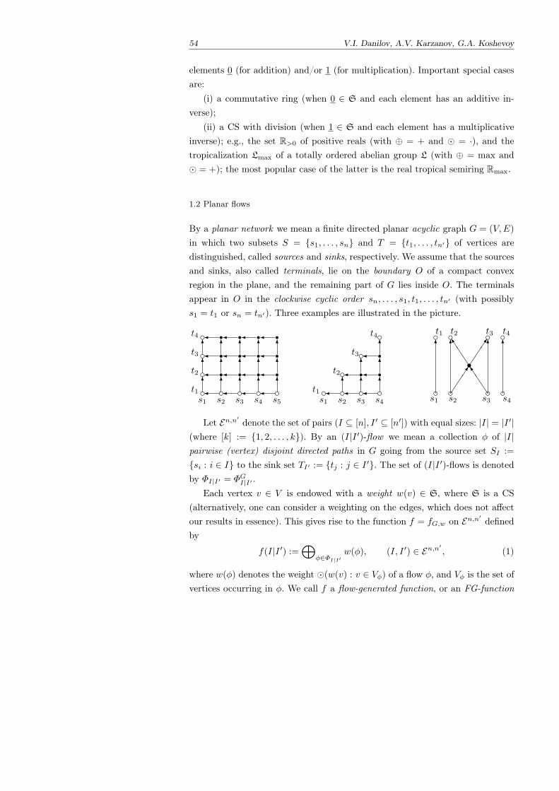
54 V.I. Danilov, A.V. Karzanov, G.A. Koshevoy
elements 0 (for addition) and/or 1 (for multiplication). Important special casesare:
(i) a commutative ring (when 0 ∈ S and each element has an additive in-verse);
(ii) a CS with division (when 1 ∈ S and each element has a multiplicativeinverse); e.g., the set R>0 of positive reals (with ⊕ = + and ⊙ = ·), and thetropicalization Lmax of a totally ordered abelian group L (with ⊕ = max and⊙ = +); the most popular case of the latter is the real tropical semiring Rmax.
1.2 Planar flows
By a planar network we mean a finite directed planar acyclic graph G = (V,E)
in which two subsets S = s1, . . . , sn and T = t1, . . . , tn′ of vertices aredistinguished, called sources and sinks, respectively. We assume that the sourcesand sinks, also called terminals, lie on the boundary O of a compact convexregion in the plane, and the remaining part of G lies inside O. The terminalsappear in O in the clockwise cyclic order sn, . . . , s1, t1, . . . , tn′ (with possiblys1 = t1 or sn = tn′). Three examples are illustrated in the picture.
c c c c cc r r r rc r r r rc r r r r
6
6
6
6
6
6
6
6
6
6
6
6
6
6
6
s1 s2 s3 s4 s5
t1
t2
t3
t4
c c c cc r rc rc
6
6
6
6
6
6
s1 s2 s3 s4
t1
t2
t3
t4
c c c c
c c c cs6 6 6 6
JJ
J]
JJ
J]
s1 s2 s3 s4
t1 t2 t3 t4
Let En,n′denote the set of pairs (I ⊆ [n], I ′ ⊆ [n′]) with equal sizes: |I| = |I ′|
(where [k] := 1, 2, . . . , k). By an (I|I ′)-flow we mean a collection ϕ of |I|pairwise (vertex) disjoint directed paths in G going from the source set SI :=
si : i ∈ I to the sink set TI′ := tj : j ∈ I ′. The set of (I|I ′)-flows is denotedby ΦI|I′ = ΦGI|I′ .
Each vertex v ∈ V is endowed with a weight w(v) ∈ S, where S is a CS(alternatively, one can consider a weighting on the edges, which does not affectour results in essence). This gives rise to the function f = fG,w on En,n′
definedby
f(I|I ′) :=⊕
ϕ∈ΦI|I′w(ϕ), (I, I ′) ∈ En,n
′, (1)
where w(ϕ) denotes the weight ⊙(w(v) : v ∈ Vϕ) of a flow ϕ, and Vϕ is the set ofvertices occurring in ϕ. We call f a flow-generated function, or an FG-function
Planar Flows and Quadratic Relations 55
for short, and say that f is determined by G,w. The set of such functions overall corresponding G and w (with n, n′,S fixed) is denoted by FGn,n′(S).
Remark 1. When S = R, (1) is specified as f(I|I ′) :=∑ϕ∈ΦI|I′
(∏v∈Vϕ
w(v)),and when S = Rmax, (1) turns into f(I|I ′) := maxϕ∈ΦI|I′ (
∑v∈Vϕ
w(v)). In theformer (latter) case, we refer to f as an algebraic (resp. tropical) FG-function.
Remark 2. Note that an (I|I ′)-flow in G may not exist, making f(I|I ′) undefinedif S does not contain 0. To overcome this trouble, we formally extend S, whenneeded, by adding an “extra neutral” element ∗, setting ∗⊕ a = a and ∗⊙ a = ∗for all a ∈ S. In the extended semiring, one defines f(I|I ′) := ∗ in case ΦI|I′ = ∅.
When an (I|I ′)-flow ϕ enters the first |I| =: k sinks (i.e. I ′ = [k]), we saythat ϕ is a flag flow for I. Accordingly, notation ΦI| [k] is abbreviated to ΦI , andf(I| [k]) to f(I). When we are interested in the flag case only, f is regarded asa function on the set 2[n] of subsets of [n].
1.3 Lindstrom’s lemma
Assume that weights w of vertices of G belong to a commutative ringand consider the n′ × n matrix M whose entries mji are defined as∑ϕ∈Φi|j
(∏v∈Vϕ
w(v)) (cf. Remark 1). For (I, I ′) ∈ En,n′, let fM (I|I ′) de-
note the minor of M with the column set I and the row set I ′. A remarkableproperty shown by Lindstrom [7] is that fM = fG,w.
(Note that the class of matrices whose minor functions are flow-generated islarge. In particular, it has been shown that any totally nonnegative matrix (a realmatrix whose all minors are nonnegative) is such; see [1]. The question whetherthis class contains all matrices over any commutative ring is still open, but we canshow that it contains any matrix over a field ; see Arxiv:1102.2578v2[math.CO].)
1.4 Quadratic relations
Minors of (real or complex) matrices obey many quadratic relations. Most pop-ular among them are quadratic relations on flag minors, or Plucker relations(which, in particular, describe flag manifolds and Grassmannians embedded incorresponding projective spaces). Therefore, by Lindstrom’s lemma, similar re-lations should be valid for any FG-function f = fG,w when S = R or C (or evenan arbitrary commutative ring). Below are two examples.
56 V.I. Danilov, A.V. Karzanov, G.A. Koshevoy
(i) The simplest example of Plucker relations (in the flag case) involve triples:for any three elements i < j < k in [n] and any subset X ⊆ [n]− i, j, k,
f(Xik)f(Xj) = f(Xij)f(Xk) + f(Xjk)f(Xi), (2)
where for brevity we write Xi′ . . . j′ for X ∪ i′, . . . , j′ (and as before, f(I)stands for f(I| [|I|])). This is called the AP3-relation (abbreviating “algebraicPlucker relation with triples").
(ii) The simplest relation in the non-flag case arises from Dodgson’s conden-sation formula for matrices [3]: for elements i < k of [n] and elements i′ < k′ of[n′] and for X ⊆ [n]− i, k and X ′ ⊆ [n′]− i′, k′,
f(iX| i′X ′) f(Xk|X ′k′) = f(iXk| i′X ′k′) f(X|X ′) + f(iX|X ′k′) f(Xk| i′X ′).
(3)
The “tropical counterpart” of (2) is the TP3-relation, viewed as
f(Xik) + f(Xj) = maxf(Xij) + f(Xk), f(Xjk) + f(Xi). (4)
This is valid for any tropical FG-function f ; see [2] (where the case S = Rmax
is considered, but the argument is extended straightforwardly to any Lmax).
In general, the quadratic relations of our interest involve FG-functions onEn,n′
over an arbitrary CS S and can be expressed as⊕(A,A′)∈A
(f(XA|X ′A′)⊙ f(XA|X ′A ′)
)=⊕
(B,B′)∈B
(f(XB|X ′B′)⊙ f(XB|X ′B ′)
). (5)
Here: X,Y (resp. X ′, Y ′) are disjoint subsets of [n] (resp. [n′]); we write KL forK ∪ L; the complement Y − C of C ⊆ Y is denoted by C, and the complementY ′ − C ′ of C ′ ⊆ Y ′ by C ′. The families A,B consist of certain pairs (C ⊆Y,C ′ ⊆ Y ′), admitting multiple ones. (The sizes of sets above are assumed to beagreeable: they should satisfy |X|+ |C| = |X ′|+ |C ′| and |X|+ |C| = |X ′|+ |C ′|,or, equivalently, 2|X|+ |Y | = 2|X ′|+ |Y ′| and |Y | − 2|C| = |Y ′| − 2|C ′|.)
In fact, an instance of (5) represents a variety of relations of “the same type”,which does not depend on X,Y,X ′, Y ′ and is specified by two patterns A0 andB0. More precisely, letting m := |Y | and m′ := |Y ′|, take the order preservingmaps γ : [m] → Y and γ′ : [m′] → Y ′ (i.e. γ(i) < γ(j) for i < j, and similarly forγ′). Then the pattern A0 (inducing A) consists of pairs (A0 ⊆ [m], A′
0 ⊆ [m′])
so that A = (γ(A0), γ′(A′
0)) : (A0, A′0) ∈ A0), and the pattern B0 (inducing B)
is defined similarly. We write A = γY,Y ′(A0) and B = γY,Y ′(B0).
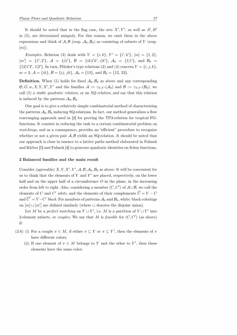
Planar Flows and Quadratic Relations 57
It should be noted that in the flag case, the sets X ′, Y ′, as well as A′, B′
in (5), are determined uniquely. For this reason, we omit them in the aboveexpressions and think of A,B (resp. A0,B0) as consisting of subsets of Y (resp.[m]).
Examples. Relation (3) deals with Y = i, k, Y ′ = i′, k′, [m] = 1, 2,[m′] = 1′, 2′, A = i|i′, B = ik|i′k′, i|k′, A0 = 1|1′, and B0 =
12|1′2′, 1|2′. In turn, Plucker’s type relations (2) and (4) concern Y = i, j, k,m = 3, A = ik, B = ij, jk, A0 = 13, and B0 = 12, 23.
Definition. When (5) holds for fixed A0,B0 as above and any correspondingS, G,w,X, Y,X ′, Y ′ and the families A := γY,Y ′(A0) and B := γY,Y ′(B0), wecall (5) a stable quadratic relation, or an SQ-relation, and say that this relationis induced by the patterns A0,B0.
Our goal is to give a relatively simple combinatorial method of characterizingthe patterns A0,B0 inducing SQ-relations. In fact, our method generalizes a flowrearranging approach used in [2] for proving the TP3-relation for tropical FG-functions. It consists in reducing the task to a certain combinatorial problem onmatchings, and as a consequence, provides an “efficient” procedure to recognizewhether or not a given pair A,B yields an SQ-relation. It should be noted thatour approach is close in essence to a lattice paths method elaborated in Fulmekand Kleber [5] and Fulmek [4] to generate quadratic identities on Schur functions.
2 Balanced families and the main result
Consider (agreeable) X,Y,X ′, Y ′,A,B,A0,B0 as above. It will be convenient forus to think that the elements of Y and Y ′ are placed, respectively, on the lowerhalf and on the upper half of a circumference O in the plane, in the increasingorder from left to right. Also, considering a member (C,C ′) of A∪B, we call theelements of C and C ′ white, and the elements of their complements C = Y −C
and C′= Y −C ′ black. For members of patterns A0 and B0, white/black colorings
on [m] ⊔ [m′] are defined similarly (where ⊔ denotes the disjoint union).Let M be a perfect matching on Y ⊔ Y ′, i.e. M is a partition of Y ⊔ Y ′ into
2-element subsets, or couples. We say that M is feasible for (C,C ′) (as above)if:
(2.6) (i) For a couple π ∈ M , if either π ⊆ Y or π ⊆ Y ′, then the elements of πhave different colors;
(ii) If one element of π ∈ M belongs to Y and the other to Y ′, then theseelements have the same color;
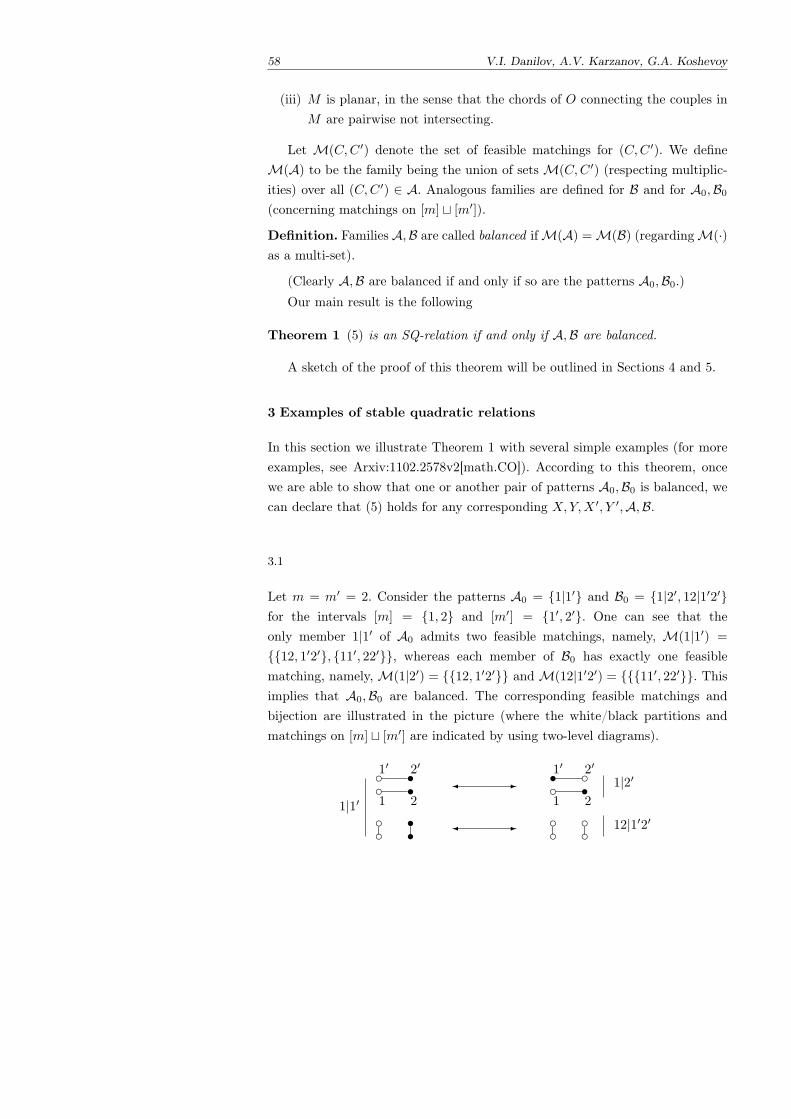
58 V.I. Danilov, A.V. Karzanov, G.A. Koshevoy
(iii) M is planar, in the sense that the chords of O connecting the couples inM are pairwise not intersecting.
Let M(C,C ′) denote the set of feasible matchings for (C,C ′). We defineM(A) to be the family being the union of sets M(C,C ′) (respecting multiplic-ities) over all (C,C ′) ∈ A. Analogous families are defined for B and for A0,B0
(concerning matchings on [m] ⊔ [m′]).
Definition. Families A,B are called balanced if M(A) = M(B) (regarding M(·)as a multi-set).
(Clearly A,B are balanced if and only if so are the patterns A0,B0.)
Our main result is the following
Theorem 1 (5) is an SQ-relation if and only if A,B are balanced.
A sketch of the proof of this theorem will be outlined in Sections 4 and 5.
3 Examples of stable quadratic relations
In this section we illustrate Theorem 1 with several simple examples (for moreexamples, see Arxiv:1102.2578v2[math.CO]). According to this theorem, oncewe are able to show that one or another pair of patterns A0,B0 is balanced, wecan declare that (5) holds for any corresponding X,Y,X ′, Y ′,A,B.
3.1
Let m = m′ = 2. Consider the patterns A0 = 1|1′ and B0 = 1|2′, 12|1′2′for the intervals [m] = 1, 2 and [m′] = 1′, 2′. One can see that theonly member 1|1′ of A0 admits two feasible matchings, namely, M(1|1′) =
12, 1′2′, 11′, 22′, whereas each member of B0 has exactly one feasiblematching, namely, M(1|2′) = 12, 1′2′ and M(12|1′2′) = 11′, 22′. Thisimplies that A0,B0 are balanced. The corresponding feasible matchings andbijection are illustrated in the picture (where the white/black partitions andmatchings on [m] ⊔ [m′] are indicated by using two-level diagrams).
c sc sc sc s1 2
1′ 2′
c cc cc ss c1 2
1′ 2′
1|1′
12|1′2′
1|2′
-
-
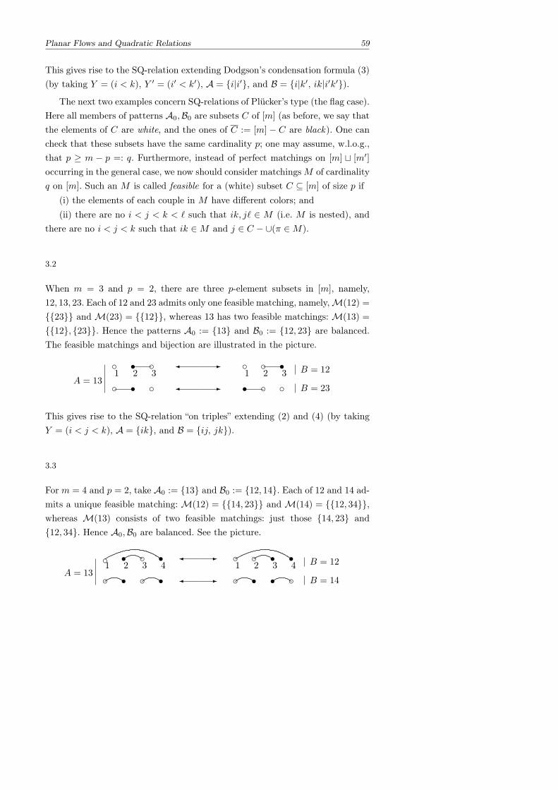
Planar Flows and Quadratic Relations 59
This gives rise to the SQ-relation extending Dodgson’s condensation formula (3)(by taking Y = (i < k), Y ′ = (i′ < k′), A = i|i′, and B = i|k′, ik|i′k′).
The next two examples concern SQ-relations of Plucker’s type (the flag case).Here all members of patterns A0,B0 are subsets C of [m] (as before, we say thatthe elements of C are white, and the ones of C := [m] − C are black). One cancheck that these subsets have the same cardinality p; one may assume, w.l.o.g.,that p ≥ m − p =: q. Furthermore, instead of perfect matchings on [m] ⊔ [m′]
occurring in the general case, we now should consider matchingsM of cardinalityq on [m]. Such an M is called feasible for a (white) subset C ⊆ [m] of size p if
(i) the elements of each couple in M have different colors; and(ii) there are no i < j < k < ℓ such that ik, jℓ ∈ M (i.e. M is nested), and
there are no i < j < k such that ik ∈M and j ∈ C − ∪(π ∈M).
3.2
When m = 3 and p = 2, there are three p-element subsets in [m], namely,12, 13, 23. Each of 12 and 23 admits only one feasible matching, namely, M(12) =
23 and M(23) = 12, whereas 13 has two feasible matchings: M(13) =
12, 23. Hence the patterns A0 := 13 and B0 := 12, 23 are balanced.The feasible matchings and bijection are illustrated in the picture.
cc
cc c
cc
css
ss
-
-1 2 3 1 2 3
A = 13B = 23
B = 12
This gives rise to the SQ-relation “on triples” extending (2) and (4) (by takingY = (i < j < k), A = ik, and B = ij, jk).
3.3
For m = 4 and p = 2, take A0 := 13 and B0 := 12, 14. Each of 12 and 14 ad-mits a unique feasible matching: M(12) = 14, 23 and M(14) = 12, 34,whereas M(13) consists of two feasible matchings: just those 14, 23 and12, 34. Hence A0,B0 are balanced. See the picture.
cc
cc c
cc
css
ss
s ss s
-
-1 2 3 4 1 2 3 4
A = 13B = 14
B = 12
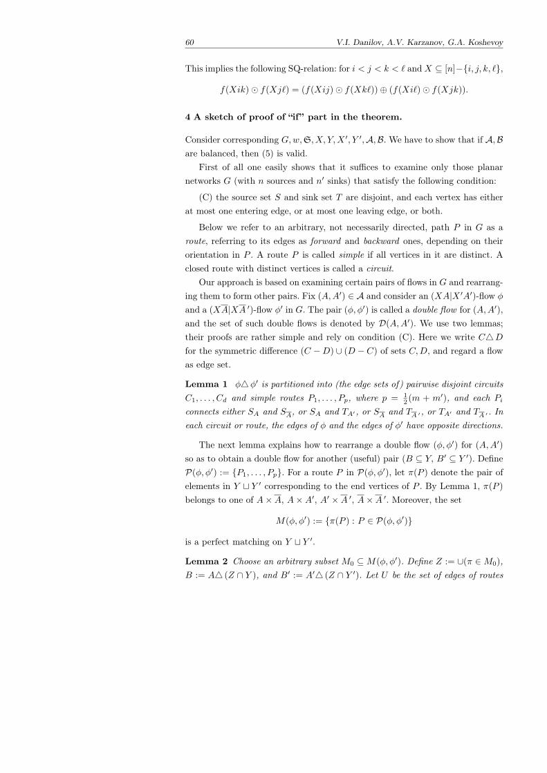
60 V.I. Danilov, A.V. Karzanov, G.A. Koshevoy
This implies the following SQ-relation: for i < j < k < ℓ andX ⊆ [n]−i, j, k, ℓ,
f(Xik)⊙ f(Xjℓ) = (f(Xij)⊙ f(Xkℓ))⊕ (f(Xiℓ)⊙ f(Xjk)).
4 A sketch of proof of “if” part in the theorem.
Consider corresponding G,w,S, X, Y,X ′, Y ′,A,B. We have to show that if A,Bare balanced, then (5) is valid.
First of all one easily shows that it suffices to examine only those planarnetworks G (with n sources and n′ sinks) that satisfy the following condition:
(C) the source set S and sink set T are disjoint, and each vertex has eitherat most one entering edge, or at most one leaving edge, or both.
Below we refer to an arbitrary, not necessarily directed, path P in G as aroute, referring to its edges as forward and backward ones, depending on theirorientation in P . A route P is called simple if all vertices in it are distinct. Aclosed route with distinct vertices is called a circuit.
Our approach is based on examining certain pairs of flows in G and rearrang-ing them to form other pairs. Fix (A,A′) ∈ A and consider an (XA|X ′A′)-flow ϕ
and a (XA|XA ′)-flow ϕ′ in G. The pair (ϕ, ϕ′) is called a double flow for (A,A′),and the set of such double flows is denoted by D(A,A′). We use two lemmas;their proofs are rather simple and rely on condition (C). Here we write CD
for the symmetric difference (C −D) ∪ (D − C) of sets C,D, and regard a flowas edge set.
Lemma 1 ϕϕ′ is partitioned into (the edge sets of) pairwise disjoint circuitsC1, . . . , Cd and simple routes P1, . . . , Pp, where p = 1
2 (m + m′), and each Pi
connects either SA and SA, or SA and TA′ , or SA and TA ′ , or TA′ and TA ′ . Ineach circuit or route, the edges of ϕ and the edges of ϕ′ have opposite directions.
The next lemma explains how to rearrange a double flow (ϕ, ϕ′) for (A,A′)
so as to obtain a double flow for another (useful) pair (B ⊆ Y, B′ ⊆ Y ′). DefineP(ϕ, ϕ′) := P1, . . . , Pp. For a route P in P(ϕ, ϕ′), let π(P ) denote the pair ofelements in Y ⊔ Y ′ corresponding to the end vertices of P . By Lemma 1, π(P )belongs to one of A×A, A×A′, A′ ×A ′, A×A ′. Moreover, the set
M(ϕ, ϕ′) := π(P ) : P ∈ P(ϕ, ϕ′)
is a perfect matching on Y ⊔ Y ′.
Lemma 2 Choose an arbitrary subset M0 ⊆M(ϕ, ϕ′). Define Z := ∪(π ∈M0),B := A (Z ∩ Y ), and B′ := A′ (Z ∩ Y ′). Let U be the set of edges of routes
Planar Flows and Quadratic Relations 61
P ∈ P(ϕ, ϕ′) with π(P ) ∈ M0. Then ψ := ϕU gives an (XB|X ′B′)-flow, andψ′ := ϕ′U gives an (XB|X ′B ′)-flow. Also ψ ⊔ ψ′ = ϕ ⊔ ϕ′.
Obviously, M(ψ,ψ′) = M(ϕ, ϕ′) and P(ψ,ψ′) = P(ϕ, ϕ′), and the transfor-mation of ψ,ψ′ by use of the routes P ∈ P(ψ,ψ′) with π(P ) ∈ M0 returnsϕ, ϕ′.
Now consider the FG-function f = fG,w on En,n′. The summand concerning
(A,A′) ∈ A in the L.H.S. of (5) can be expressed via double flows as follows:
f(XA|X ′A′)⊙ f(XA|X ′A ′)
=
(⊕ϕ∈ΦXA|X′A′
w(ϕ)
)⊙(⊕
ϕ′∈ΦXA|X′A ′w(ϕ′)
)(7)
=⊕
(ϕ,ϕ′)∈D(A,A′)w(ϕ)⊙ w(ϕ′)
=⊕
M∈M(A,A′)
⊕(ϕ,ϕ′)∈D(A,A′) : M(ϕ,ϕ′)=M
w(ϕ)⊙ w(ϕ′).
The summand concerning (B,B′) ∈ B in the L.H.S. of (5) is expressed similarly.Finally, for (A,A′) ∈ A and M ∈ M(A,A′), consider (ϕ, ϕ′) ∈ D(A,A′) such
that M(ϕ, ϕ′) =M (if it exists). Since A,B are balanced, (A,A′,M) is bijectiveto some (B,B′,M) such that (B,B′) ∈ B and M ∈ M(B,B′). Since M is afeasible matching for both (A,A′) and (B,B′), it follows from (6)(i),(ii) that(B,B′) is obtained from (A,A′) by “recoloring” w.r.t. some M0 ⊆M . Then thetransformation of (ϕ, ϕ′) by use of the routes P ∈ P(ϕ, ϕ′) with π(P ) ∈ M0
(as described in Lemma 2), results in a double flow (ψ,ψ′) for (B,B′) such thatψ⊔ψ′ = ϕ⊔ϕ′, implying w(ψ)⊙w(ψ′) = w(ϕ)⊙w(ϕ′). Moreover, (ϕ, ϕ′) 7→ (ψ,ψ′)
gives a bijection between all double flows for (A,A′,M) and those for (B,B′,M).Now (5) follows by considering the last term in (7).
5 Necessity of the balancedness
Part “only if” of Theorem 1 says that if patterns A0,B0 are not balanced, thenthere exist corresponding G,w,S, X, Y,X ′, Y ′ for which (5) with A = γY,Y ′(A0)
and B = γY,Y ′(B0) is violated. (Hereinafter X,Y are disjoint subsets of [n],X ′, Y ′ are disjoint subsets of [n′], and X,Y,X ′, Y ′,A0,B0 should be agreeable,i.e. there hold m+2|X| = m′+2|X ′| and m−2|C| = m′−2|C ′| for all (C,C ′) ∈A0∪B0, where m := |Y |, m′ := |Y ′|.) We can show a sharper result, saying thatif the patterns are not balanced, then (5) is violated for any choice of X,Y,X ′, Y ′
and for S := Z+.
62 V.I. Danilov, A.V. Karzanov, G.A. Koshevoy
Proposition 1 Suppose that patterns A0,B0 are not balanced. Fix (agreeable)X,Y,X ′, Y ′. Then there exists, and can be explicitly constructed, a planar net-work G = (V,E) such that (5) is false for f = fG,w, where w(v) = 1 for allv ∈ V .
The idea of the proof is roughly as follows. Since A0,B0 are not balanced,there exists a planar perfect matching M on Y ⊔ Y ′ such that
|AM | = |BM |,
where AM is the set of members of A having M as a feasible matching, andsimilarly for B. We succeed to construct a planar network G (depending onX,Y,X ′, Y ′,M) with the following properties: for any pair (C ⊆ Y, C ′ ⊆ Y ′),
(P1) If M ∈ M(C,C ′), then G has a unique (XC|X ′C ′)-flow and a unique(XC|X ′C ′)-flow, i.e. |ΦXC|X′C′ | = |ΦXC|X′C ′ | = 1;
(P2) If M /∈ M(C,C ′), then at least one of ΦXC|X′C′ and ΦXC|X′C ′ is empty.
Take the function f = fG,w for w ≡ 1. By (P1) and (P2), for a pair (C,C ′),each of the values f(XC|X ′C ′) and f(XC|X ′C ′) is equal to 1 if M ∈ M(C,C ′),and at least one of them is 0 otherwise. This implies that the values in the L.H.S.and R.H.S. of (5) are exactly |AM | and |BM |, respectively. Thus, these valuesare different and (5) is violated.
6 Applications to Schur functions
It is known that Schur functions (polynomials) are expressed as minors of a cer-tain matrix, by Jacobi–Trudi’s formula. Therefore, these functions satisfy manyquadratic relations. [4, 5] and some other works (see a discussion in [4]) explainhow to obtain quadratic relations for ordinary and skew Schur functions by useof a lattice paths method based on the Gessel–Viennot interpretation of semis-tandard Young tableaux [6]. This lattice path method is, in fact, a specializationto a particular planar network of the flow approach that we described in Sec-tions 1,2. Below we give a brief discussion on this subject.
Recall that a partition of length r is an r-tuple λ of weakly decreasing non-negative integers λ1 ≥ λ2 ≥ . . . ≥ λr. The Ferrers diagram of λ is meant tobe the array Fλ of cells with r left-aligned rows containing λi cells in ith row.(We assume that the row indices grow from the bottom to the top.) For N ∈ N,an N -semistandard Young tableau of shape λ is a filling T of Fλ with naturalnumbers not exceeding N so that the numbers weakly increase in each row andstrictly increase in each column. We associate to T the monomial xT to be the
Planar Flows and Quadratic Relations 63
product of variables x1, . . . , xN , each xk being taken with the degree equal tothe number of occurrences of k in T . Then the Schur function for λ and N isthe polynomial
sλ = sλ(x1, . . . , xN ) :=∑
TxT ,
where the sum is over all N -semistandard Young tableaux T of shape λ. Besides,one often considers a skew Schur function sλ/µ, where µ is a partition of lengthr with µi ≤ λi; it is defined in a similar way w.r.t. the skew Ferrers diagramFλ/µ obtained by removing from Fλ the cells of Fµ. When needed, an “ordinary”diagram Fλ is regarded as Fλ/µ with µ = (0, . . . , 0), and similarly for tableaux.
There is a one-to-one correspondence between the partitions λ of length r
and the r-element subsets Aλ of the set Z>0 of positive integers, namely:
λ = (λ1 ≥ . . . ≥ λr) ⇐⇒ Aλ := λr + 1, λr−1 + 2, . . . , λ1 + r. (8)
The graph of our interest is the directed square grid Γ = Γ (N) whose verticesare the points (i, j) for i ∈ Z>0 and j ∈ [N ] and whose edges e are directed up orto the right, i.e. e = ((i, j), (i, j+1)) or ((i, j), (i+1, j)) (it suffices to take a finitetruncation of this grid). The vertices si := (i, 1) and ti := (i,N) are regarded asthe sources and sinks in Γ , respectively, and we assign to each horizontal edge eat level h the weight to be the indeterminate xh:
w(e) := xh for e = ((i, h), (i+ 1, h)), i ∈ Z>0, h = 1, . . . , N , (9)
and assign weight 1 to each vertical edge. Now using the Gessel–Viennotmodel [6] (in a slightly different form), one can associate to an N -semistandardskew Young tableau T with shape λ/µ the system PT = (P1, . . . , Pr) of directedpaths in Γ , where for k = 1, . . . , r:
(6.10) Pk is related to (r+1− k)th row of T : it goes from the source sk+µr+1−kto
the sink tk+λr+1−k, and for h = 1, . . . , N , the number of horizontal edges of
Pk at level h equals the number of occurrences of h in kth row of T .
So the sources occurring in PT are the si for i ∈ Aµ, and the sinks are the tjfor j ∈ Aλ. Observe that the semistandardness of T implies that these paths arepairwise disjoint, i.e. PT is an (Aµ|Aλ)-flow in Γ . One can see the converse aswell: if P is an (Aµ|Aλ)-flow in Γ , then the filling T of Fλ/µ determined, in a dueway, by the horizontal edges of paths in P is just a semistandard skew Youngtableau, and one has PT = P. This gives a nice bijection between correspondingflows and tableaux. The next picture illustrates an example of a semistandardYoung tableau T with N = 6, r = 5, λ = (6, 5, 3, 3, 2) and µ = (2, 2, 1, 1, 0), andits corresponding flow PT = (P1, . . . , P5).
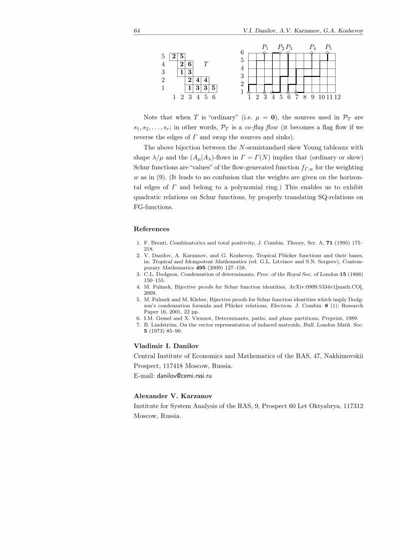
64 V.I. Danilov, A.V. Karzanov, G.A. Koshevoy
1 2 3 4 5 612345
1 3 3 52 4 4
1 32 6
2 5T
c c c c c
c c c c c
1 2 3 4 5 6 7 8 9 10 11 12123456
P1 P2P3 P4 P5
Note that when T is “ordinary” (i.e. µ = 0), the sources used in PT ares1, s2, . . . , sr; in other words, PT is a co-flag flow (it becomes a flag flow if wereverse the edges of Γ and swap the sources and sinks).
The above bijection between the N -semistandard skew Young tableaux withshape λ/µ and the (Aµ|Aλ)-flows in Γ = Γ (N) implies that (ordinary or skew)Schur functions are “values” of the flow-generated function fΓ,w for the weightingw as in (9). (It leads to no confusion that the weights are given on the horizon-tal edges of Γ and belong to a polynomial ring.) This enables us to exhibitquadratic relations on Schur functions, by properly translating SQ-relations onFG-functions.
References
1. F. Brenti, Combinatorics and total positivity, J. Combin. Theory, Ser. A, 71 (1995) 175–218.
2. V. Danilov, A. Karzanov, and G. Koshevoy, Tropical Plucker functions and their bases,in: Tropical and Idempotent Mathematics (ed. G.L. Litvinov and S.N. Sergeev), Contem-porary Mathematics 495 (2009) 127–158.
3. C.L. Dodgson, Condensation of determinants, Proc. of the Royal Soc. of London 15 (1866)150–155.
4. M. Fulmek, Bijective proofs for Schur function identities, ArXiv:0909.5334v1[math.CO],2009.
5. M. Fulmek and M. Kleber, Bijective proofs for Schur function identities which imply Dodg-son’s condensation formula and Plucker relations, Electron. J. Combin. 8 (1): ResearchPaper 16, 2001, 22 pp.
6. I.M. Gessel and X. Viennot, Determinants, paths, and plane partitions, Preprint, 1989.7. B. Lindstrom, On the vector representation of induced matroids, Bull. London Math. Soc.
5 (1973) 85–90.
Vladimir I. DanilovCentral Institute of Economics and Mathematics of the RAS, 47, NakhimovskiiProspect, 117418 Moscow, Russia.E-mail: [email protected]
Alexander V. KarzanovInstitute for System Analysis of the RAS, 9, Prospect 60 Let Oktyabrya, 117312Moscow, Russia.

E-mail: [email protected]
Gleb A. KoshevoyCentral Institute of Economics and Mathematics of the RAS, 47, NakhimovskiiProspect, 117418 Moscow, Russia.E-mail: [email protected]
Tropical and Idempotent Mathematics. Moscow, Russia, August 26–31, 2012
Tropical Plucker functions and Kashiwaracrystals of types A, B, and C
Vladimir I. DanilovAlexander V. KarzanovGleb A. Koshevoy
1 Introduction
Kashiwara [K90] introduced the fundamental notion of a crystal in represen-tation theory. This is an edge-colored directed graph in which each connectedmonochromatic subgraph is a finite path and there are certain interrelations onthe lengths of such paths, described in terms of a Cartan matrix M ; this matrixcharacterizes the type of a crystal. An important class of crystals is formed by thecrystals of representations, or regular crystals; these are associated to irreduciblehighest weight integrable modules (representations) over the quantum envelop-ing algebra related to M . There are several models to characterize the regularcrystals for a variety of types; e.g., via generalized Young tableaux [KN94], Lit-telmann’s path model [Lt95], MV-polytopes [K].
Here we propose a new model of crystals for the Cartan matrix of type A. Inthis model, the set of vertices of the crystal is the set of integer-valued tropicalPlucker functions on the Boolean cube 2[n+1]. To decide if a pair of functions fand g is connected by an edge of some color i, we have to restrict f and g toa surface (the union of certain 2-faces in the Boolean cube which correspond tosome rhombus tiling) adopted to i.
This model is symmetric on the colors (see Section 5). This allows us toobtain regular crystals for the Cartan matrices of Dynkin Bn- and Cn-types assymmetric extracts from crystals of A2n−1- and A2n-types, respectively. Notethat among the above-mentioned models, Littelmann’s path model and Kam-nitzer’s MV-polytope model are also symmetric, and this property was used
Plucker functions and crystals 67
in [H] and [NS] for construction crystals of B- and C-types as symmetric ex-tracts from A-types; a direct combinatorial proof, based on the so-called crossingmodel, is given in [DKK12].
There are other advantages of our model. Firstly, it is not too intricate andprovides a new viewpoint on Young tableaux of B and C types. Secondly, usingour model, we obtain an explicit description of the principal lattice of crystals oftypes A, B and C. The principal lattice in A-type crystals was introduced andstudied in [DKK08].
In Section 2 we recall some basic facts on tropical Plucker functions (TP-functions). In Section 3 we define a structure of пїЅ free crystal on the set ofTP-functions. In Section 4 we consider ’bounded’ subcrystals (intervals) in aconnected free crystal. In the last Section 5, we explain how crystals of Bm- andCm-types can be derived from symmetric TP-functions on 2[2m] and 2[2m+1],respectively.
2 Tropical Plucker functions
1. For a positive integer n, let [n] denote the set 1, 2, . . . , n. A real-valuedfunction f on the set of subsets of [n], that is a function on the Boolean cube2[n], is said to be a tropical Plucker function, or a TP-function, if it satisfies theTP3-relation
f(Aik) + f(Aj) = maxf(Aij) + f(Ak), f(Ai) + f(Ajk), (1)
for any triple i < j < k in [n] and subset A ⊆ [n] − i, j, k, where for brevitywe write Ai′ . . . j′ instead of A ∪ i′, . . . , j′.
The set of integer-valued TP-functions on 2[n] is denoted by TPn (the set ofreal-valued functions is denoted by TPn(R)).
2. The set TPn is a subset of the space R2[n]
of all functions on 2[n]. TPn(R)is stable under multiplication on positive numbers. It is not stable under summa-tion, however, the polyhedral conic complex TPn(R) contains a lineal of principalTP-functions of the dimension 2n. The lineal is constituted from sums of affinefunctions and functions which depend only on cardinalities of sets.
3. Definition. A subset B ⊆ 2[n] is called a TP-basis, or simply a basis, ifthe restriction map res : TPn(R) → RB is a bijection. In other words, eachTP-function is determined by its values on B, and moreover, values on B canbe chosen arbitrarily.
68 V.I. Danilov, A.V. Karzanov, G.A. Koshevoy
Such bases do exist and, for our aims here, we consider bases of the form ofspectra of rhombus tiling diagrams. Let us recall the notion of a tiling diagram(for details, see [DKK10]).
Tiling diagrams live within a zonogon, which is defined as follows. In theupper half-plane, take n non-colinear vectors ξ1 = (a1, 1), . . . , ξn = (an, 1) sothat a1 < a2 < . . . < an. Then the set Z = Zn := λ1ξ1 + . . .+ λnξn : 0 ≤ λi ≤1, i = 1, . . . , n is a 2n-gone. Moreover, Z is a zonogon, as it is the sum of n line-segments λξi : 1 ≤ λ ≤ 1, i = 1, . . . , n. It is the image of the solid cube [0, 1][n]
into the plane R2 by a linear projection π, defined by π(x) := x1ξ1 + . . .+ xnξn.The boundary of Z consists of two parts: the left boundary, lbd(Z), formed by thepoints (vertices) zℓi := ξ1+ . . .+ξi (i = 0, . . . , n), and the right boundary, rbd(Z),formed by the points zri := ξi+1+ . . .+ ξn (i = 0, . . . , n). The points zℓ0 = zrn andzℓn = zr0 are the minimal vertex and the maximal vertex of Z correspondingly.
A subset X ⊆ [n] is identified with the corresponding vertex of the n-cubeand with the point
∑i∈X ξi in the zonogon Z.
By a tile (or a rhombus) we mean a parallelogram τ of the form X + λξi +λ′ξj : 0 ≤ λ, λ′ ≤ 1, where X ⊂ [n] and 1 ≤ i < j ≤ n; we also call it anij-tile at X and denote by τ(X; i, j). According to a natural visualization of τ ,its vertices X,Xi,Xj,Xij are called the bottom, left, right, top vertices of τ anddenoted by b(τ), ℓ(τ), r(τ), t(τ), respectively. Also we say that a point (subset)Y ⊆ [n] is of height |Y |.
4. Definition. A tiling diagram, or a tiling for short, is a collection T of tilesτ(X; i, j) which forms a polyhedral decomposition of Zn.
A vertex (an edge) of a tiling T is a vertex (an edge) of some rhombus of T .Thus the set of vertices of T defines a collection of corresponding subsets in 2[n].Such a collection of subsets is the spectrum of the tiling T , Sp(T ). Note thatboundary vertices of Zn, ∅, 1, 1, 2,..., 1, 2, ..., n, 2, ..., n,..., n, belongto the spectrum of every tiling.
5. For any tiling T , the spectrum Sp(T ) is a TP-basis (see [DKK10]). Thebijection
TPn(R) → RSp(T )
is a piecewise linear map. One can consider tilings as charts of an atlas forTPn. The transformation maps between charts take the form of sequences ofTP3-relations (1); see [DKK10].
Plucker functions and crystals 69
6. Let R be a tile τ(A; i, j). Then an excess of a function f : 2[n] → R in therhombus R is said to be the amount
ε(f,R) = f(Ai) + f(Aj)− f(A)− f(Aij).
Any functions on vertices of a tiling T is defined by its values at the vertices onthe right boundary of Zn and the excesses at tiles of T .
3 Free crystal of type A
1. A digraph K = (V (K), E(K)) is an n edge-colored if E(K) = E1 ⊔ . . . ⊔ En,where any edge e ∈ Ei has a color 1. An edge-colored digraph K is a pre-crystalif two following axioms are satisfied. The first axiom requires that, for any colori, the subgraph (V (K), Ei) is a disjoin union of strings (finite or infinite). Atranslation along an edge of a color i is understood as an action of the operationi on the set V (K). Namely, if an edge (v, u) has color i, then i(v) = u, and wesay that the operation i acts at v. If, for a vertex v there is no edge of color iemanating from v, then we say that i does not act at v.
The reversing edges of the graph K defines the reverse operations i−1. Theseoperations are inverse in the following sense: if i acts at v and w = iv, then i−1
acts at w and v = i−1w.
Example. A commutative pre-crystal is an Abelian group Z[n] on which anoperator i sends x to x+ 1i, where 1i is the i-th basis vector.
Let K and K ′ be two n-colored pre-crystals. A morphism K → K ′ is amapping φ : V (K) → V (K ′) which commutes with the actions of operations i,that is if i does act at v in the pre-crystal K, then i acts at φ(v) and there holdsφ(iv) = iφ(v).
The second axiom of pre-crystals requires the existence of a weight map, amorphism wt : K → Z[n].
2. Crystals are associated to (generalized) Cartan matrices. Let M = (mij),i, j ∈ [n] be a (generalized) Cartan matrix, that is mij ∈ Z, mii = 2, andmij ≤ 0 for i = j. For a pre-crystal to be a crystal, more axioms, which relatethe weight map and Cartan data, have to be satisfied. However, according to2-color reduction theorem [KKMMNN], a ’bounded’ pre-crystal is a crystal ofan integrable M -module iff the restriction of K to any pair of colors i, j is acrystal of the corresponding M |ij-module. For simply- and doubly-laced cases,it suffices to know crystals of three types A1 + A1, A2 and B2. A structure ofsuch crystals are studied in depth, for example, in [DKK07,DKK09].
70 V.I. Danilov, A.V. Karzanov, G.A. Koshevoy
3. Let us define a structure of pre-crystal with n colors on the vertex set beinginteger-valued TP-functions TP = TPn+1(Z) on 2[n+1] (as we will see later sucha pre-crystal is an An-crystal indeed). We need several notions.
Let us call a tile τ of a tiling T a left rhombus if it shares 2 edges with theleft boundary of the zonogon Zn+1. Specifically, τ is a left-rhombus at the heighth if b(τ) = [h− 1],l(τ) = [h], and t(τ) = [h+ 1]. Denote such a rhombus tile byLRh. Analogously a right rhombus RRh at the height h is defined.
We say that a tiling T (in the zonogon Z = Zn+1) is fitted to the color i(i = 1, . . . , n), if T contains the left rhombus LRi.For any color i, there exists atiling which is fitted to i
4. Now all is ready to define a crystal operation i (i = 1, . . . , n) at a TP-function f ∈ TPn+1. Pick a tiling T , which is fitted to the color i. Then thefunction if is defined (see 2.5) by the rule
(if)(v) =
f(v) + 1, if v = [i],
f(v) otherwise.
In other words, in the chart T the function if differs from f in the single vertex[i] of T . However, the functions f and if may be different at some other verticesof the Boolean cube. Nevertheless, they coincide at the vertices of the rightboundary rbd(Zn+1).
5. Theorem. The operations i (i = 1, ..., n) are correctly defined and theyendow the set TP = TPn+1 with a structure of an An-crystal.
According to 2-color reduction theorem [KKMMNN], we have to considerthe case n = 3. In such a case one can establish an explicit bijection with thecrossing model for A2-crystal from [DKK07].
6. The crystal operations i commute with addition of any (integer-valued)principal TP-function. That is, for any TP-function f and any principal TP-function p, there holds
i(f + p) = if + p.
7. As we remarked above the crystal actions preserve values of TP-functions atthe vertices at rbd(Zn+1). Thus, the values at these vertices are n+2 ’integrals’,and any connected component of crystal TPn+1 is specified by x ∈ Zn+2, a listof values at the vertices of rbd(Z). Denote by K[x] such a crystal. Since, fordifferent x, the crystals K[x] are isomorphic. We consider a crystal K = K[0]
with the vertices being integer-valued TP-functions which are equal to zero atany vertex of rbd(Zn+1).
Plucker functions and crystals 71
8. Consider the subset P of principal TP-functions which belong to K. Thatis the set of principal TP-functions which equal 0 at the vertices of rbd(Z).Because of 2.8, we may specify the excesses of such a function for rhombuses ateach height. Thus, we get an isomorphism between P and the Abelian group Zn.The basis of the lattice P is constituted from the principal functions p1, . . . , pn,where the i-th function pi is specified by the following conditions:
1. equal 0 at each vertex of rbd(Z);2. for any height j = i, and any rhombus R at the height j, ε(pi, R) = 0;3. for any rhombus R at the height i, ε(pi, R) = 1.
4 Subcrystals of K
1. Since the operations i and i−1 act at each vertex of K, the crystal K is afree crystal, that is all monochromatic strings are infinite. Here we interested insubsets of K which are An-type crystals.
Let us define a (partial) order ≼ on the vertices of K. For functions f , g ∈ K,we write f ≼ g if there exists a word w in the alphabet 1, . . . ,n such thatthere holds g = wf . In other words, f ≼ g if there exists a path in the digraphK emanated from f and ended in g.
For a principal vertex p ∈ K, we denote by Kp (and Kp) the set f ∈ K, p ≼f (and f ∈ K, f ≼ p). The vertex p is a single source in the poset Kp (thesingle sink in the poset Kp). We have
Kp = p+K0 and Kq = q +K0.
Because of this, we are interested in the sets K0 and K0.
2. Here is an alternative definition of the set K0. Recall, that a functionf : 2[n+1] → R is submodular, if, for any rhombus R, there holds ε(f,R) ≥ 0. Itis not difficult to prove that a TP-function f is submodular iff, for some tilingT and every tile τ ∈ T , there holds ε(f, τ) ≥ 0.
3. Theorem. The set K0 is the set of integer-valued submodular TP-functionswhich equal to 0 at rbd(Zn+1).
4. The intersection K0 and the lattice of principal TP-functions P ∼= Zn
is the semi-group Zn+. In fact, because of (3.8), every principal function pi, i =1, . . . , n, is submodular. Moreover, only non-negative linear combinations of thesefunctions are submodular.
5. We get the following corollary from Theorem 4.3
72 V.I. Danilov, A.V. Karzanov, G.A. Koshevoy
Corollary. The crystal K is connected.
If fact, let us show that any function of K is of the form w 0, where w is aword in the alphabet 1±1, . . . ,n±1. Specifically, for any f ∈ K, we can find aprincipal function p ∈ P such that the TP-function f + p is submodular. Then,according to Theorem 4.3, there exists a word w in the alphabet 1, . . . ,n suchthat there holds f+p = w0. Hence f = w(−p). Since, due to Theorem 4.3, thereexists a word v such that p = v0, we have have −p = v−10. All this impliesf = wv−10.
6. Here we give a description of the set K0 using excesses.
Theorem. A TP-function f ∈ K belongs to K0 iff, for every right rhombusRRi, there holds ε(f,RRi) ≤ 0.
Let p ∈ P ∩K be a principal function. Then a function f ∈ K belongs to Kp
iff, for any i = 1, . . . , n, there holds ε(f,RRi) ≤ ε(p,RRi) .
7. The crystals of the form of an interval, Kpq = Kp ∩ Kq, where p, q ∈ P
and q ≼ p, correspond to finite-dimensional integrable modules. Wlog, we mayconsider q = 0. The graph Kp
0 is connected, has finitely many vertices, a singlesource 0 and a single sink p.
Because of Theorem 4.3 and 4.6, a function f ∈ K belongs to the crystalKp
0 = K0 ∩Kp (with some p ∈ P ) iff
1. For any rhombus R, there holds ε(f,R) ≥ 0;2. for any right rhombus RRi, i = 1, . . . , n, there holds ε(f,RRi) ≤ ε(p,RRi).
The intersection of a crystal Kp0 and the principal lattice P is constituted
from the functions of the form∑i cipi, where 0 ≤ ci ≤ ε(p,RRi), that is an
integer parallelepiped. For a tuple c = (c1, ..., cn) ∈ Zn≥0, we denote by K(c) thecrystal Kp
0 , where p =∑i cn+1−ipi.
8. Proposition. 1) ci is equal to the maximal number α such that a functioniα0 belongs to K(c).
2) cn−i+1 is equal to the maximal number β such that a function i−βp belongsto K(c).
5 Symmetric extracts from symmetric A-crystals
1. The inversion σ(i) = n + 2 − i of the set [n + 1] can be considered as aninversion of the Dynkin diagram An. Consider the inversion γ of the Booleancube 2[n+1], defined by γ(A) = σ([n+ 1]−A).
Plucker functions and crystals 73
Consider an extension of the inversion γ to the zonogon Z = Zn+1. For this,consider symmetric (w.r.t. σ) vectors ξi = (xi, 1), that is ξn+2−i = (−xi, 1).Denote by γ the symmetry of the plane w.r.t. the horizontal line y = (n+ 2)/2.This symmetry sends Z to itself: if a point v ∈ Z corresponds to a subsetA ⊂ [n+1], then the point γ(v) corresponds to the subset γ(A). This symmetryextends to the space of functions on the Boolean cube. Namely, let f : 2[n+1] → Rbe a function on the Boolean cube. Then the function γ∗f : 2[n+1] → R sendsa set A to f(γ(A)). Obviously, f is a TP-function if and only if γ∗f is a TP-function.
Denote by TP the set of symmetric TP-functions, γ∗f = f . We are going toendow the set TP with a crystal structure. This depends on the parity of n.
2. Let n be odd, n = 2m−1, m ≥ 1. In this case there are plenty of symmetrictilings. A tiling T is symmetric if its set of vertices and edges is stable under thesymmetry γ, i.e. γT = T .
In this case, any symmetric TP-function defines a symmetric function on anysymmetric tiling, and vice versa. Consider m operations 1, . . . , m on TP , where1 = 1n = n1, . . . , m− 1 = (m − 1)(m + 1), m = m, where 1, . . . ,n are thecrystal operations on TP . These operations can be defined as follows. For anoperation i, we consider a symmetric tiling T fitted to the color i. Then, by thesymmetry, T also is fitted to the color n + 1 − i = 2m − i. The operation i onthe vertices of T is defined by the rule
(if)(v) =
f(v) + 1, if v = [i] or [2m− i]
f(v) otherwise.
Note that for i = m, we have [m] = [2m−m], and the operation m increases by1 the value of a function at the symmetric vertex [m].
3. Theorem. TP is a free Bm-crystal.
4. Considering symmetric functions in the subcrystals K0, K0 and K(c), withsymmetric c (cσ(i) = ci, i = 1, . . . ,m) of type A2m−1, we obtain Bm-subcrystalsin the free Bm-crystal TP . The symmetric part of K(c) of K(c) is an interval inthe poset K consisting of symmetric TP-functions between the principal vertices0 and p =
∑2m+1i=1 cipi.
Let us consider simplest examples for n = 3. The A3-crystal K(0, 1, 0) isdrawn in the left part of the picture below. The symmetric vertices are indicatedby bold circles, and the extracted B2-crystal K(0, 1) is depicted in the right part.
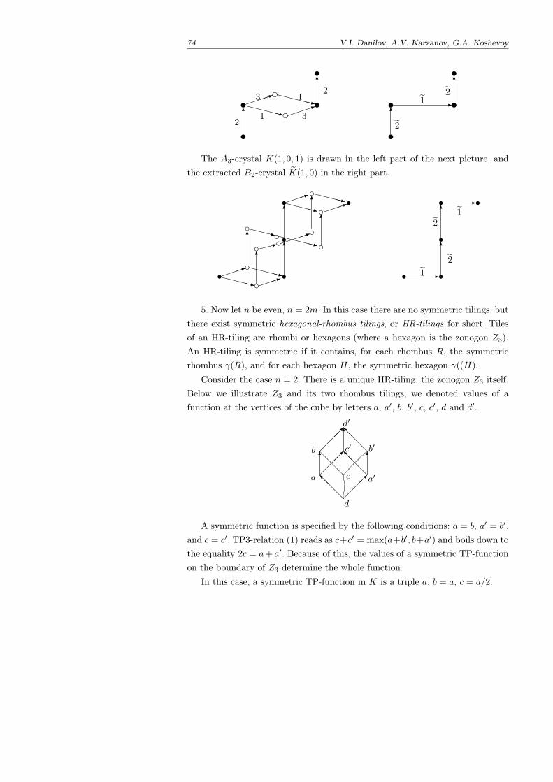
74 V.I. Danilov, A.V. Karzanov, G.A. Koshevoy
t6tXXXXXz d1 dXXXXXz
1 t6t
21
3 1
3
2
tt t
t6
-
6
2
12
The A3-crystal K(1, 0, 1) is drawn in the left part of the next picture, andthe extracted B2-crystal K(1, 0) in the right part.
s cc sss sc cc cc c c c
1XXXXz 1
XXXXz
6
6XXXXz1 XXXXz
1
6: 1
6
6XXXz XXXXXz
6
s sss s
-
6
6-
1
2
21
5. Now let n be even, n = 2m. In this case there are no symmetric tilings, butthere exist symmetric hexagonal-rhombus tilings, or HR-tilings for short. Tilesof an HR-tiling are rhombi or hexagons (where a hexagon is the zonogon Z3).An HR-tiling is symmetric if it contains, for each rhombus R, the symmetricrhombus γ(R), and for each hexagon H, the symmetric hexagon γ((H).
Consider the case n = 2. There is a unique HR-tiling, the zonogon Z3 itself.Below we illustrate Z3 and its two rhombus tilings, we denoted values of afunction at the vertices of the cube by letters a, a′, b, b′, c, c′, d and d′.
@@@I
6
@
@@I
6
6@
@@I
a
b
c
c′
d
d′
a′
b′
A symmetric function is specified by the following conditions: a = b, a′ = b′,and c = c′. TP3-relation (1) reads as c+c′ = max(a+b′, b+a′) and boils down tothe equality 2c = a+ a′. Because of this, the values of a symmetric TP-functionon the boundary of Z3 determine the whole function.
In this case, a symmetric TP-function in K is a triple a, b = a, c = a/2.
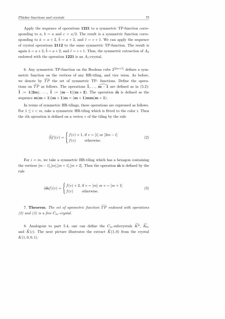
Plucker functions and crystals 75
Apply the sequence of operations 1221 to a symmetric TP-function corre-sponding to a, b = a and c = a/2. The result is a symmetric function corre-sponding to a = a + 2, b = a + 2, and c = c + 1. We can apply the sequenceof crystal operations 2112 to the same symmetric TP-function. The result isagain a = a+ 2, b = a+ 2, and c = c+ 1. Thus, the symmetric extraction of A2
endowed with the operation 1221 is an A1-crystal.
6. Any symmetric TP-function on the Boolean cube 2[2m+1] defines a sym-metric function on the vertices of any HR-tiling, and vice versa. As before,we denote by TP the set of symmetric TP- functions. Define the opera-tions on TP as follows. The operations 1,. . . , m− 1 are defined as in (5.2):1 := 1(2m), . . . , 1 := (m− 1)(m+ 2). The operation m is defined as thesequence m(m+ 1)(m+ 1)m = (m+ 1)mm(m+ 1).
In terms of symmetric HR-tilings, these operations are expressed as follows.For 1 ≤ i < m, take a symmetric HR-tiling which is fitted to the color i. Thenthe ith operation is defined on a vertex v of the tiling by the rule
(if)(v) =
f(v) + 1, if v = [i] or [2m− i]
f(v) otherwise.(2)
For i = m, we take a symmetric HR-tiling which has a hexagon containingthe vertices [m− 1],[m],[m+ 1],[m+ 2]. Then the operation m is defined by therule
(mf)(v) =
f(v) + 2, if v = [m] or v = [m+ 1]
f(v) otherwise.(3)
7. Theorem. The set of symmetric function TP endowed with operations(2) and (3) is a free Cm-crystal.
8. Analogous to part 5.4, one can define the Cm-subcrystals K0, K0,and K(c). The next picture illustrates the extract K(1, 0) from the crystalK(1, 0, 0, 1).
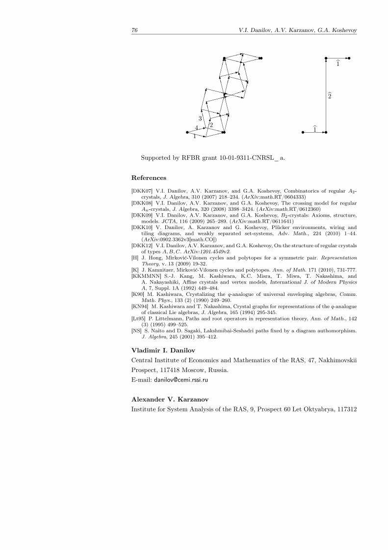
76 V.I. Danilov, A.V. Karzanov, G.A. Koshevoy
XXXz:CCCCOCCCO:XXXz
:XXXzCCCOCCCOXXXz:
CCCO:1B
BBM
CCCOXXXXzXXXz
CCCO
:XXXz
:XXXz
s s
s s
14 23
-
6-
1
2
1
s s
s s
Supported by RFBR grant 10-01-9311-CNRSL_ a.
References
[DKK07] V.I. Danilov, A.V. Karzanov, and G.A. Koshevoy, Combinatorics of regular A2-crystals, J. Algebra, 310 (2007) 218–234. (ArXiv:math.RT/0604333)
[DKK08] V.I. Danilov, A.V. Karzanov, and G.A. Koshevoy, The crossing model for regularAn-crystals, J. Algebra, 320 (2008) 3398–3424. (ArXiv:math.RT/0612360)
[DKK09] V.I. Danilov, A.V. Karzanov, and G.A. Koshevoy, B2-crystals: Axioms, structure,models. JCTA, 116 (2009) 265–289. (ArXiv:math.RT/0611641)
[DKK10] V. Danilov, A. Karzanov and G. Koshevoy, Plucker environments, wiring andtiling diagrams, and weakly separated set-systems, Adv. Math., 224 (2010) 1–44.(ArXiv:0902.3362v3[math.CO])
[DKK12] V.I. Danilov, A.V. Karzanov, and G.A. Koshevoy, On the structure of regular crystalsof types A,B,C. ArXiv:1201.4549v2.
[H] J. Hong, Mirkovic-Vilonen cycles and polytopes for a symmetric pair. RepresentationTheory, v. 13 (2009) 19-32.
[K] J. Kamnitzer, Mirkovic-Vilonen cycles and polytopes. Ann. of Math. 171 (2010), 731-777.[KKMMNN] S.-J. Kang, M. Kashiwara, K.C. Misra, T. Miwa, T. Nakashima, and
A. Nakayashiki, Affine crystals and vertex models, International J. of Modern PhysicsA, 7, Suppl. 1A (1992) 449–484.
[K90] M. Kashiwara, Crystalizing the q-analogue of universal enveloping algebras, Comm.Math. Phys., 133 (2) (1990) 249–260.
[KN94] M. Kashiwara and T. Nakashima, Crystal graphs for representations of the q-analogueof classical Lie algebras, J. Algebra, 165 (1994) 295-345.
[Lt95] P. Littelmann, Paths and root operators in representation theory, Ann. of Math., 142(3) (1995) 499–525.
[NS] S. Naito and D. Sagaki, Lakshmibai-Seshadri paths fixed by a diagram authomorphism.J. Algebra, 245 (2001) 395–412.
Vladimir I. DanilovCentral Institute of Economics and Mathematics of the RAS, 47, NakhimovskiiProspect, 117418 Moscow, Russia.E-mail: [email protected]
Alexander V. KarzanovInstitute for System Analysis of the RAS, 9, Prospect 60 Let Oktyabrya, 117312

Moscow, Russia.E-mail: [email protected]
Gleb A. KoshevoyCentral Institute of Economics and Mathematics of the RAS, 47, NakhimovskiiProspect, 117418 Moscow, Russia.E-mail: [email protected]
Tropical and Idempotent Mathematics. Moscow, Russia, August 26–31, 2012
Discriminant of system of equations
A. Esterov
1. Introduction
What polynomial in the coefficients of a system of algebraic equations shouldbe called its discriminant? We prove a package of facts that provide a possibleanswer. Let us call a system typical, if the homeomorphic type of its set ofsolutions does not change as we perturb its (non-zero) coefficients. The set of allatypical systems turns out to be a hypersurface in the space of all systems of kequations in n ≥ k−1 variables, whose monomials are contained in k given finitesets. This hypersurface B is the union of two well-known strata: the set of allsystems that have a singular solution (this stratum is conventionally called thediscriminant) and the set of all systems, whose principal part is degenerate (theycan be regarded as systems with a singular solution at infinity). None of these twostrata is a hypersurface in general, and codimensions of their components havenot been fully understood yet (e.g. dual defect toric varieties are not classified), sothe purity of dimension of their union seems somewhat surprising. We deduce itfrom a similar tropical purity fact of independent interest: the stable intersectionof a tropical fan with a boundary of a polytope in the ambient space has purecodimension one in this tropical fan.
A generic system of equations in an irreducible component Bi of the hyper-surface B always differs from a typical system by the Euler characteristic of itsset of solutions. Regarding the difference of these two Euler characteristics asthe multiplicity of Bi, we turn B into an effective divisor, whose equation wecall the Euler discriminant of a system of equations by the following reasons.Firstly, it vanishes exactly at those systems that have a singular solution (pos-
Discriminant of system of equations 79
sibly at infinity). Secondly, despite its topological definition, it admits a simplelinear-algebraic formula for its computation, and a positive formula for its New-ton polytope. Thirdly, it interpolates many classical objects and inherits many oftheir nice properties: for k = n+1, it is the sparse resultant (defined by vanishingon consistent systems of equations); for k = 1, it is the principal A-determinant(defined as the sparse resultant of the polynomial and its partial derivatives); aswe specialize the indeterminate coefficients of our system to be polynomials ofa new parameter, the Euler discriminant turns out to be preserved under thisbase change, similarly to discriminants of deformations. This allows, for exam-ple, to specialize our results to generic polynomial maps: the bifurcation set ofa dominant polynomial map, whose components are generic linear combinationsof given monomials, is always a hypersurface, and a generic atypical fiber of sucha map differs from a typical one by its Euler characteristic.
2. Degenerate systems
For a finite set H ⊂ Zn, we study the space C[H] of all Laurent polynomialsh(x) =
∑a∈H cax
a, where xa stands for the monomial xa11 . . . xann , the coefficientca is a complex number, and the polynomial h is considered as a function (C \0)n → C. For a linear function v : Zn → Z, denote the intersection of H with theboundary of the affine half-space H + v < 0 by Hv, and the highest v-degreecomponent
∑a∈Hv cax
a by hv (if v = 0, then we set H0 = H and h0 = h).
In what follows, we denote a collection of finite sets A0, . . . , Ak in Zn by A, thespace C[A0]⊕ . . .⊕ C[Ak] by C[A], consider its element f = (f0, . . . , fk) ∈ C[A]as a map (C \ 0)n → Ck+1, and denote (fv0 , . . . , f
vk ) by fv.
Theorem 1 Assume that A0+ . . .+Ak is not contained in an affine hyperplane.The following three conditions are equivalent for the system of equations f = 0:1) There exists an arbitrarily small f ∈ C[A], such that the sets f = 0 andf + f = 0 are not diffeomorphic.2) There exists an arbitrarily small f ∈ C[A], such that the sets f = 0 andf + f = 0 have different Euler characteristic.3) There exists a linear function v : Zn → Z such that the differentialsdfv0 , . . . , df
vk are linearly dependent at some point of the set fv = 0.
The assumption on A0 + . . . + Ak cannot be dropped, because, otherwise, theEuler characteristic of f = 0 equals 0 for every f ∈ C[A] by homogeneityconsiderations.
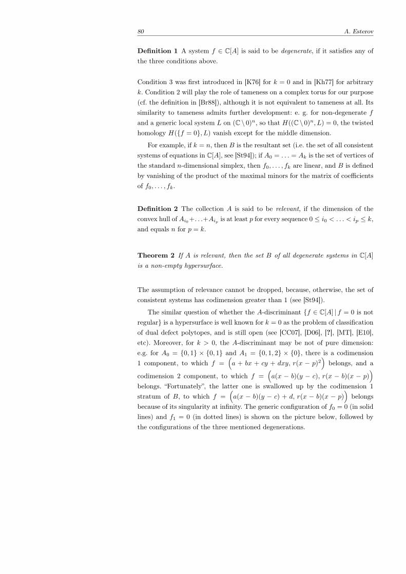
80 A. Esterov
Definition 1 A system f ∈ C[A] is said to be degenerate, if it satisfies any ofthe three conditions above.
Condition 3 was first introduced in [K76] for k = 0 and in [Kh77] for arbitraryk. Condition 2 will play the role of tameness on a complex torus for our purpose(cf. the definition in [Br88]), although it is not equivalent to tameness at all. Itssimilarity to tameness admits further development: e. g. for non-degenerate fand a generic local system L on (C \ 0)n, so that H((C \ 0)n, L) = 0, the twistedhomology H(f = 0, L) vanish except for the middle dimension.
For example, if k = n, then B is the resultant set (i.e. the set of all consistentsystems of equations in C[A], see [St94]); if A0 = . . . = Ak is the set of vertices ofthe standard n-dimensional simplex, then f0, . . . , fk are linear, and B is definedby vanishing of the product of the maximal minors for the matrix of coefficientsof f0, . . . , fk.
Definition 2 The collection A is said to be relevant, if the dimension of theconvex hull of Ai0+. . .+Aip is at least p for every sequence 0 ≤ i0 < . . . < ip ≤ k,and equals n for p = k.
Theorem 2 If A is relevant, then the set B of all degenerate systems in C[A]is a non-empty hypersurface.
The assumption of relevance cannot be dropped, because, otherwise, the set ofconsistent systems has codimension greater than 1 (see [St94]).
The similar question of whether the A-discriminant f ∈ C[A] | f = 0 is notregular is a hypersurface is well known for k = 0 as the problem of classificationof dual defect polytopes, and is still open (see [CC07], [D06], [?], [MT], [E10],etc). Moreover, for k > 0, the A-discriminant may be not of pure dimension:e.g. for A0 = 0, 1 × 0, 1 and A1 = 0, 1, 2 × 0, there is a codimension1 component, to which f =
(a + bx + cy + dxy, r(x − p)2
)belongs, and a
codimension 2 component, to which f =(a(x − b)(y − c), r(x − b)(x − p)
)belongs. “Fortunately”, the latter one is swallowed up by the codimension 1stratum of B, to which f =
(a(x − b)(y − c) + d, r(x − b)(x − p)
)belongs
because of its singularity at infinity. The generic configuration of f0 = 0 (in solidlines) and f1 = 0 (in dotted lines) is shown on the picture below, followed bythe configurations of the three mentioned degenerations.
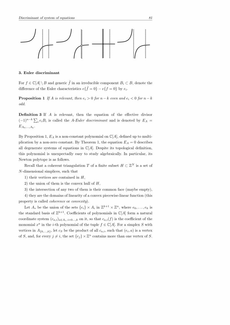
Discriminant of system of equations 81
3. Euler discriminant
For f ∈ C[A] \B and generic f in an irreducible component Bi ⊂ B, denote thedifference of the Euler characteristics ef = 0 − ef = 0 by ei.
Proposition 1 If A is relevant, then ei > 0 for n−k even and ei < 0 for n−kodd.
Definition 3 If A is relevant, then the equation of the effective divisor(−1)n−k
∑i eiBi is called the A-Euler discriminant and is denoted by EA =
EA0,...,Ak.
By Proposition 1, EA is a non-constant polynomial on C[A], defined up to multi-plication by a non-zero constant. By Theorem 1, the equation EA = 0 describesall degenerate systems of equations in C[A]. Despite its topological definition,this polynomial is unexpectadly easy to study algebraically. In particular, itsNewton polytope is as follows.
Recall that a coherent triangulation T of a finite subset H ⊂ ZN is a set ofN -dimensional simplices, such that
1) their vertices are contained in H,2) the union of them is the convex hull of H,3) the intersection of any two of them is their common face (maybe empty),4) they are the domains of linearity of a convex piecewise-linear function (this
property is called coherence or convexity).Let A∗ be the union of the sets ei × Ai in Zk+1 × Zn, where e0, . . . , ek is
the standard basis of Zk+1. Coefficients of polynomials in C[A] form a naturalcoordinate system (ca,i)a∈Ai, i=0...,k on it, so that ca,i(f) is the coefficient of themonomial xa in the i-th polynomial of the tuple f ∈ C[A]. For a simplex S withvertices in A0,...,k, let cS be the product of all ca,i, such that (ei, a) is a vertexof S, and, for every j = i, the set ej×Zn contains more than one vertex of S.
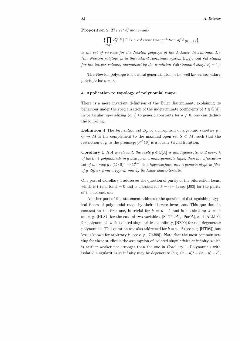
82 A. Esterov
Proposition 2 The set of monomials∏S∈T
cVolSS |T is a coherent triangulation of A0,...,k
is the set of vertices for the Newton polytope of the A-Euler discriminant EA(the Newton polytope is in the natural coordinate system (ca,i), and Vol standsfor the integer volume, normalized by the condition Vol(standard simplex) = 1).
This Newton polytope is a natural generalization of the well known secondarypolytope for k = 0.
4. Application to topology of polynomial maps
There is a more invariant definition of the Euler discriminant, explaining itsbehaviour under the specialization of the indeterminate coefficients of f ∈ C[A].In particular, specializing (ca,i) to generic constants for a = 0, one can deducethe following.
Definition 4 The bifurcation set Bp of a morphism of algebraic varieties p :
Q → M is the complement to the maximal open set S ⊂ M , such that therestriction of p to the preimage p−1(S) is a locally trivial fibration.
Corollary 1 If A is relevant, the tuple g ∈ C[A] is nondegenerate, and every kof the k+1 polynomials in g also form a nondegenerate tuple, then the bifurcationset of the map g : (C\0)n → Ck+1 is a hypersurface, and a generic atypical fiberof g differs from a typical one by its Euler characteristic.
One part of Corollary 1 addresses the question of purity of the bifurcation locus,which is trivial for k = 0 and is classical for k = n − 1: see [J93] for the purityof the Jelonek set.
Another part of this statement addresses the question of distinguishing atyp-ical fibers of polynomial maps by their discrete invariants. This question, incontrast to the first one, is trivial for k = n − 1 and is classical for k = 0:see e. g. [HL84] for the case of two variables, [SieTib95], [Par95], and [ALM00]for polynomials with isolated singularities at infinity, [NZ90] for non-degeneratepolynomials. This question was also addressed for k = n−2 (see e. g. [HT08]),butless is known for arbitrary k (see e. g. [Gaf99]). Note that the most common set-ting for these studies is the assumption of isolated singularities at infinity, whichis neither weaker nor stronger than the one in Corollary 1. Polynomials withisolated singularities at infinity may be degenerate (e.g. (x− y)2 + (x− y) + c),
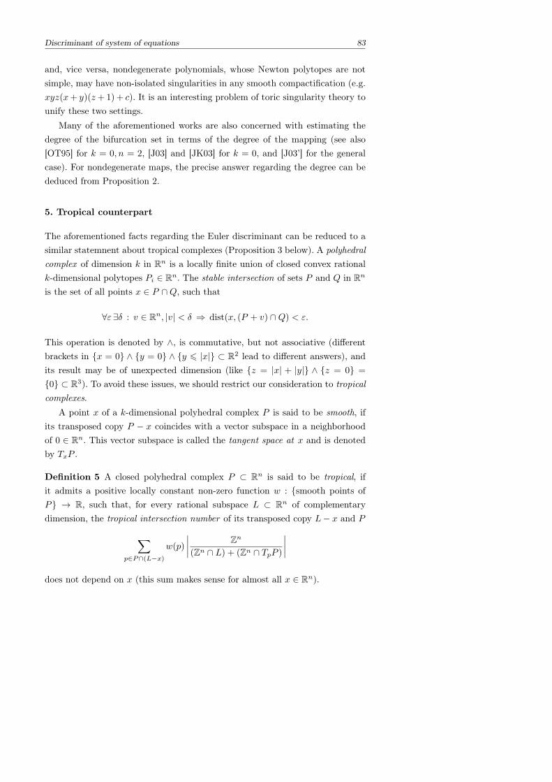
Discriminant of system of equations 83
and, vice versa, nondegenerate polynomials, whose Newton polytopes are notsimple, may have non-isolated singularities in any smooth compactification (e.g.xyz(x+ y)(z+1)+ c). It is an interesting problem of toric singularity theory tounify these two settings.
Many of the aforementioned works are also concerned with estimating thedegree of the bifurcation set in terms of the degree of the mapping (see also[OT95] for k = 0, n = 2, [J03] and [JK03] for k = 0, and [J03’] for the generalcase). For nondegenerate maps, the precise answer regarding the degree can bededuced from Proposition 2.
5. Tropical counterpart
The aforementioned facts regarding the Euler discriminant can be reduced to asimilar statemnent about tropical complexes (Proposition 3 below). A polyhedralcomplex of dimension k in Rn is a locally finite union of closed convex rationalk-dimensional polytopes Pi ∈ Rn. The stable intersection of sets P and Q in Rn
is the set of all points x ∈ P ∩Q, such that
∀ε ∃δ : v ∈ Rn, |v| < δ ⇒ dist(x, (P + v) ∩Q) < ε.
This operation is denoted by ∧, is commutative, but not associative (differentbrackets in x = 0 ∧ y = 0 ∧ y 6 |x| ⊂ R2 lead to different answers), andits result may be of unexpected dimension (like z = |x| + |y| ∧ z = 0 =
0 ⊂ R3). To avoid these issues, we should restrict our consideration to tropicalcomplexes.
A point x of a k-dimensional polyhedral complex P is said to be smooth, ifits transposed copy P − x coincides with a vector subspace in a neighborhoodof 0 ∈ Rn. This vector subspace is called the tangent space at x and is denotedby TxP .
Definition 5 A closed polyhedral complex P ⊂ Rn is said to be tropical, ifit admits a positive locally constant non-zero function w : smooth points ofP → R, such that, for every rational subspace L ⊂ Rn of complementarydimension, the tropical intersection number of its transposed copy L− x and P
∑p∈P∩(L−x)
w(p)
∣∣∣∣ Zn
(Zn ∩ L) + (Zn ∩ TpP )
∣∣∣∣does not depend on x (this sum makes sense for almost all x ∈ Rn).
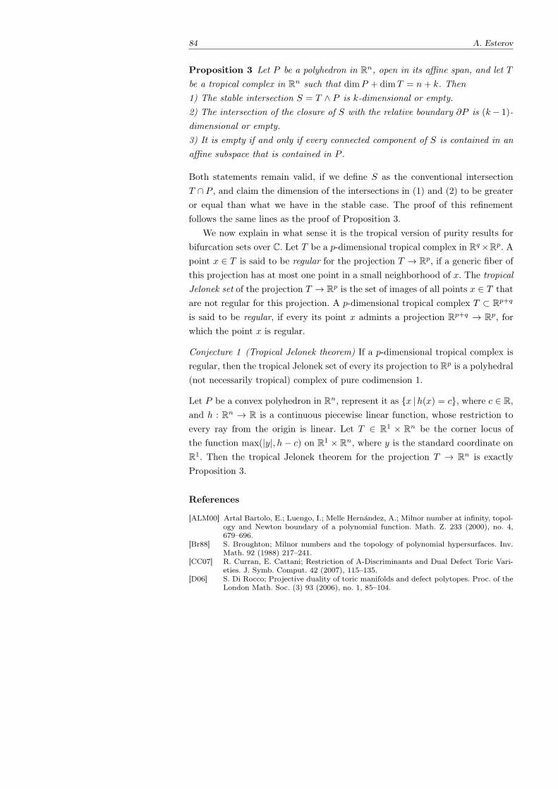
84 A. Esterov
Proposition 3 Let P be a polyhedron in Rn, open in its affine span, and let Tbe a tropical complex in Rn such that dimP + dimT = n+ k. Then1) The stable intersection S = T ∧ P is k-dimensional or empty.2) The intersection of the closure of S with the relative boundary ∂P is (k− 1)-dimensional or empty.3) It is empty if and only if every connected component of S is contained in anaffine subspace that is contained in P .
Both statements remain valid, if we define S as the conventional intersectionT ∩ P , and claim the dimension of the intersections in (1) and (2) to be greateror equal than what we have in the stable case. The proof of this refinementfollows the same lines as the proof of Proposition 3.
We now explain in what sense it is the tropical version of purity results forbifurcation sets over C. Let T be a p-dimensional tropical complex in Rq×Rp. Apoint x ∈ T is said to be regular for the projection T → Rp, if a generic fiber ofthis projection has at most one point in a small neighborhood of x. The tropicalJelonek set of the projection T → Rp is the set of images of all points x ∈ T thatare not regular for this projection. A p-dimensional tropical complex T ⊂ Rp+q
is said to be regular, if every its point x admints a projection Rp+q → Rp, forwhich the point x is regular.
Conjecture 1 (Tropical Jelonek theorem) If a p-dimensional tropical complex isregular, then the tropical Jelonek set of every its projection to Rp is a polyhedral(not necessarily tropical) complex of pure codimension 1.
Let P be a convex polyhedron in Rn, represent it as x |h(x) = c, where c ∈ R,and h : Rn → R is a continuous piecewise linear function, whose restriction toevery ray from the origin is linear. Let T ∈ R1 × Rn be the corner locus ofthe function max(|y|, h− c) on R1 × Rn, where y is the standard coordinate onR1. Then the tropical Jelonek theorem for the projection T → Rn is exactlyProposition 3.
References
[ALM00] Artal Bartolo, E.; Luengo, I.; Melle Hernandez, A.; Milnor number at infinity, topol-ogy and Newton boundary of a polynomial function. Math. Z. 233 (2000), no. 4,679–696.
[Br88] S. Broughton; Milnor numbers and the topology of polynomial hypersurfaces. Inv.Math. 92 (1988) 217–241.
[CC07] R. Curran, E. Cattani; Restriction of A-Discriminants and Dual Defect Toric Vari-eties. J. Symb. Comput. 42 (2007), 115–135.
[D06] S. Di Rocco; Projective duality of toric manifolds and defect polytopes. Proc. of theLondon Math. Soc. (3) 93 (2006), no. 1, 85–104.
[E10] A. Esterov; Newton polyhedra of discriminants of projections. Discrete Comput.Geom., 44 (2010), no. 1, 96–148, arXiv:0810.4996.
[Gaf99] T. Gaffney, Fibers of polynomial mappings at infinity and a generalized Malgrangecondition, Compositio Math. 119 (1999) 157–167.
[GKZ94] I. M. Gelfand, M. M. Kapranov, A.V.Zelevinsky; Discriminants, Resultants, andMiltidimensional Determinants. Birkhauser, 1994.
[J93] Z. Jelonek; The set of points at which the polynomial mapping is not proper. Ann.Polon. Math. 58, 259–266 (1993) MR1244397 (94i:14018)
[J03] Jelonek, Z.; On bifurcation points of a complex polynomial. Proc. Amer. Math. Soc.131 (2003), no. 5, 1361–1367.
[J03’] Jelonek, Z.; On the generalized critical values of a polynomial mapping. ManuscriptaMath. 110 (2003), no. 2, 145–157.
[JK03] Jelonek, Z., Kurdyka, K.; On asymptotic critical values of a complex polynomial. J.Reine Angew. Math. 565 (2003), 1–11.
[Kh77] A. G. Khovanskii, Newton polyhedra and the genus of complete intersections. Func.Anal. Appl., 12 (1978), 38–46.
[K76] A. G. Kouchnirenko; Polyedres de Newton et nombres de Milnor. Inv. Math. 32(1)(1976),. 1–32.
[MT] Y. Matsui K. Takeuchi; A geometric degree formula for A-discriminants and Eulerobstructions of toric varieties. Adv. Math. 226 (2011), 2040–2064.
[NZ90] Nemethi, A., Zaharia, A.; On the bifurcation set of a polynomial function and Newtonboundary. Publ. Res. Inst. Math. Sci. 26 (1990), no. 4, 681–689.
[OT95] L. Thanh, M. Oka; Estimation of the number of the critical values at infinity ofa polynomial function f : C2 → C. Publ. Res. Inst. Math. Sci. 31 (1995), no. 4,577–598.
[Par95] Parusinski, A.; On the bifurcation set of complex polynomial with isolated singular-ities at infinity. Compositio Math. 97 (1995), no. 3, 369–384.
[SieTib95] D. Siersma, M. Tibar; Singularities at infinity and their vanishing cycles. DukeMath. Journal 80, 3 (1995), 771–783.
[St94] B. Sturmfels; On the Newton polytope of the resultant. J. Algebraic Combin. 3(1994), no. 2, 207–236.
[HL84] Ha Huy Vui, Le Dung Trang; Sur la topologie des polynomes complexes. Acta Math.Vietnam. 9 (1984), no. 1, 21–32 (1985).
[HT08] Ha Huy Vui, Nguyen Tat Thang; On the topology of polynomial functions on al-gebraic surfaces in Cn. Singularities II, 61–67, Contemp. Math., 475, Amer. Math.Soc., Providence, RI, 2008.
A. EsterovNational Research University Higher School of Economics, Moscow, RussiaE-mail: [email protected]
Tropical and Idempotent Mathematics. Moscow, Russia, August 26–31, 2012
Complexity of tropical and min-pluslinear prevarieties
Dima GrigorievVladimir V. Podolskii
Abstract In the tropical algebra, a vector x is a solution to a polynomialg1(x)⊕g2(x)⊕ . . .⊕gk(x), where gi(x)’s are tropical monomials, if the minimumin mini(gi(x)) is attained at least twice. In the min-plus algebra, solutions ofsystems of equations of the form g1(x) ⊕ . . . ⊕ gk(x) = h1(x) ⊕ . . . ⊕ hl(x) arestudied. In this paper we consider computational problems related to tropicallinear system. We show that the solvability problem (both over Z and Z∪∞)and the problem of deciding the equivalence of two linear systems (both overZ and Z ∪ ∞) are equivalent under polynomial-time reductions to meanpayoff games and also equivalent to analogous problems in min-plus algebra.In particular, all these problems belong to the complexity class NP ∩ coNP.We also show that computing the dimension of the solution space of a tropicallinear system and of a min-plus linear system is NP-complete. We extend someof our results to the systems of min-plus linear inequalities.
1. Introduction
Let K be either Z, or Z∞ = Z ∪ ∞. By the tropical linear system asso-ciated with a matrix A ∈ Km×n we understand the system of expressionsmin1≤j≤naij + xj, 1 ≤ i ≤ m, or, in other words, the vector A x forx = (x1, . . . , xn). We say that x 6= (∞, . . . ,∞) is a solution to the tropical linear
Complexity of tropical and min-plus linear prevarieties 87
system if for every row 1 ≤ i ≤ m there are two columns 1 ≤ k < l ≤ n such thataik+xk = ail+xl = min1≤j≤naij+xj. Following the notation of [7], the set ofsolutions of a tropical linear system is called tropical linear prevariety. It followsfrom the analysis of [7] that this set is a union of polyhedra of possibly differentdimensions. The dimension of a tropical prevariety is the largest dimension ofpolyhedra contained in it.
Min-plus linear system associated with a pair of matrices A,B ∈ Km×n isthe system min1≤j≤naij + xj = min1≤j≤nbij + xj, 1 ≤ i ≤ m.
Min-plus linear system of inequalities associated with a pair of matricesA,B ∈ Km×n is the system min1≤j≤naij + xj ≤ min1≤j≤nbij + xj, 1 ≤i ≤ m.
In this paper we are interested in computational aspects of tropical andmin-plus algebras. The most basic motivation comes from linear algebra and,more specifically, systems of linear equations. In the case of classical algebra,the Gaussian elimination solves linear systems in polynomial time. In the caseof tropical semiring, things turn out to be more complicated and no polynomialtime algorithm is known neither for tropical linear systems, nor for min-pluslinear systems. For the tropical case it is known, however, that the problem is inthe complexity class NP∩coNP, there are also pseudopolynomial algorithms [1,4],i.e., with complexity being polynomial in the size of a system and in absolutevalues of its coefficients, and it is also known that the problem reduces to the wellknown and long standing problem mean payoff games [1]. The same is knownfor the solvability problem for min-plus linear systems, and in addition it wasproven by Bezem et al. [2] that the problem is polynomial-time equivalent tomean payoff games.
Another complexity aspect of min-plus algebra related to our consideration isthe solvability problem of min-plus systems of linear inequalities. It is known thatthe solvability problem for these systems is equivalent to mean payoff games [1].
The first result of our paper is that the solvability problem for tropical linearsystems is also equivalent to mean payoff games. Thus on one hand we charac-terize the complexity of solvability problem of tropical linear systems and on theother hand give a new reformulation of mean payoff games. In particular, ourresult means that the solvability problem for tropical linear systems is equiva-lent to the solvability problem for min-plus linear systems, establishing a closerconnection between two problems of linear algebra over the min-plus semiring.
Next we study other problems related to tropical linear systems: the problemof equivalence of two given tropical linear systems and the problem of computing
88 D. Grigoriev, V. Podolskii
the dimension of a tropical prevariety. The former problem turns out to be alsoequivalent to mean payoff games. The same statement for min-plus linear systemsis also true and follows easily from known results. The dimension problem of thetropical prevariety turns out to be NP-complete. We prove the analogous resultfor the case of min-plus linear systems and min-plus systems of inequalities.
These results are obtained for both Z and Z∞ domains (there is no obvioustranslation between these two cases).
The proofs of our results can be found on arXiv [5].
2. Preliminaries
Next we recall the definition of mean payoff games. In an instance of a meanpayoff game we are given a directed graph G = (V,E), whose vertices are dividedinto two disjoint sets V = V1 t V2, some fixed initial node v ∈ V1 and a functionw : E → Z assigning weights to the edges of G. In the beginning of the game atoken is placed in the initial vertex v. At each turn of the game, one of the twoplayers moves the token to another node of the graph. If the token is currentlyin some node u ∈ V1, then the first player can move it to any node w such that(u,w) ∈ E. If u ∈ V2, then the second player can move the token to any nodew such that (u,w) ∈ E. The game is infinite and the process of the game canbe described by the sequence of nodes v0, v1, v2, . . . which the token visits. Notethat v0 = v. The first player wins the game if
lim inft→∞
1
t
t∑i=1
w(vi−1, vi) > 0. (1)
The mean payoff game problem is to decide whether the first player has a winningstrategy. For more information on mean payoff games see survey [6].
In this paper we consider the following problems.TropSolv. Given an integer matrix A ∈ Zm×n, decide whether the correspond-ing tropical system is solvable.TropEquiv. Given two integer matrices A ∈ Zm×n, B ∈ Zk×n, decide whetherthe corresponding tropical systems over the same set of variables are equivalent.TropDim. Given an integer matrix A ∈ Zm×n and a number k ∈ N, decidewhether the dimension of the tropical prevariety corresponding to the tropicalsystem is at least k.
For all problems above there are also variants of them over Z∞, we denotethem by the subscript ∞. For local dimension of tropical prevariety (that is the
Complexity of tropical and min-plus linear prevarieties 89
dimension of the neighborhood of some point) over Z∞ in a point with someinfinite coordinates we consider just the dimension over finite coordinates only.
3. Tropical linear systems and mean payoff games
First we prove the following theorem.
Theorem 1 The problems TropSolv and TropSolv∞ are polynomially equiv-alent to mean payoff games.
In particular, it follows that the problems TropSolv and TropSolv∞ arepolynomial time equivalent to each other. The resulting proof of equivalence ofthese two purely tropical problems rather unnaturally goes through mean payoffgames. We also give a direct proof of this equivalence.
Next we prove a result on equivalence problem.
Theorem 2 The problems TropEquiv, TropEquiv∞are polynomial timeequivalent to mean payoff games.
Analogous results for min-plus linear systems follow from known results [1,2].For both min-plus and tropical linear systems we also give direct combina-
torial proofs of equivalence between solvability and equivalence problems.
4. Dimension and the tropical rank
Now we proceed to the dimension of tropical prevarieties. First we study therelation to ranks of the matrices. There are many notions of “rank” in tropicalalgebra. For instance, Develin et al. [3] studied Barvinok rank, Kapranov rankand tropical rank. For them there is a relation
tropical rank(A) ≤ Kapranov rank(A) ≤ Barvinok rank(A), (2)
for any matrix A, and all inequalities can be strict in (2) [3].We show the following result.
Lemma 1 For any matrix A ∈ Rm×n we have
n− tropical dimension(A) ≤ tropical rank(A),
and the inequality can be both tight and strict.
This lemma together with (2) shows that there is a relation between thetropical dimension and ranks of the tropical matrix, but this relation is notenough for computational needs.
90 D. Grigoriev, V. Podolskii
5. Combinatorial characterization of the dimension of the tropicalprevariety
For our characterization we will need the following definition.
Definition 1 Let A be a matrix of size m× n. We associate with it a table ofstars A∗ of the same sizem×n, where we put ∗ to the entry (i, j) iff aij = mink aik
and we leave all other entries empty.
Table A∗ captures properties of the tropical system A essential to us. Forexample, the vector x = (x1, . . . , xn) is a solution to the system A iff there areat least two stars in every row of the table (aij + xjij)∗.
Next we give a combinatorial characterization of local dimension (at a givenpoint) of a tropical prevariety in terms of the table A∗.
Definition 2 The block triangular form of size d of the matrix A is a partitionof the set of rows of A into sets R1, R2, . . . , Rd (some of the sets Ri might beempty) and a partition of the set of columns of A into nonempty sets C1, . . . , Cd
with the following properties:
1. for every i each row in Ri has at least two stars in columns Ci in A∗;2. if 1 ≤ i < j ≤ d then rows in Ri have no stars in columns Cj in A∗.
Theorem 3 For a solution x of the tropical linear system A the local dimensionof the system A in point x is equal to the maximal d such that there is a blocktriangular form of the matrix aij + xjij of size d.
The analogous fact is true for the tropical linear systems over Z∞.We also prove analogous results for min-plus linear systems of equations and
inequalities adapting the notion of block-triangular form properly.
6. Computing the dimension of tropical and min-plus linear prevari-eties is NP-complete
Theorem 4 TropDim and TropDim∞ are NP-complete.
We prove analogous results for min-plus linear systems of equations andinequalities.
Acknowledgements. The first author is grateful to Max-Planck Institut furMathematik, Bonn for its hospitality during the work on this paper.
The question on the complexity of equivalence of min-plus linear prevarietieswas posed by Vladimir Voevodsky, who encouraged the authors to study relationsbetween tropical and min-plus linear prevarieties.
References
1. M. Akian, S. Gaubert, and A. Guterman. Tropical polyhedra are equivalent to mean payoffgames. International Journal of Algebra and Computation, 22(1), 2012.
2. M. Bezem, R. Nieuwenhuis, and E. Rodrıguez-Carbonell. Hard problems in max-algebra,control theory, hypergraphs and other areas. Inf. Process. Lett., 110(4):133–138, 2010.
3. M. Develin, F. Santos, and B. Sturmfels. On the rank of a tropical matrix. Combinatorialand Computational Geometry, 52:213–242, 2005.
4. D. Grigoriev. Complexity of solving tropical linear systems. Preprint MPI fur Mathematik,Bonn, 2010-60, 2010. To appear in Computational Complexity.
5. D. Grigoriev and V. V. Podolskii. Complexity of tropical and min-plus linear prevarieties.CoRR, abs/1204.4578, 2012.
6. H. Klauck. Algorithms for parity games. In E. Gradel, W. Thomas, and T. Wilke, editors,Automata Logics, and Infinite Games, volume 2500 of Lecture Notes in Computer Science,pages 553–563. Springer Berlin / Heidelberg, 2002.
7. J. Richter-Gebert, B. Sturmfels, and T. Theobald. First steps in tropical geometry. Idem-potent Mathematics and Mathematical Physics, Contemporary Mathematics, 377:289–317,2003.
Dima GrigorievCNRS, Mathematiques, Universite de Lille, FranceE-mail: [email protected]
Vladimir V. PodolskiiSteklov Mathematical Institute, Moscow, RussiaE-mail: [email protected]
Tropical and Idempotent Mathematics. Moscow, Russia, August 26–31, 2012
The asymptotic rank of semi-groups of tropical ma-trices
Pierre GuillonZur IzhakianJean MairesseGlenn Merlet
Abstract As it is now well known, there are several notions of rank of atropical matrix, corresponding to several equivalent definitions of the rank inusual linear algebra. However, the minimum of the ranks of matrices in a closedsemigroup does not depend on the choosen notion. Let us call asymptotic rankof a semigroup be the minimum rank of elements in its closure. The asymptoticrank of a matrix is the asymptotic rank of the semigroup of its powers. We givea polynomial algorithm to check if the asymptotic rank of a finitely generatedsemigroup of matrices is the size d of the matrices. As a byproduct, thealgorithm produces a product of at most d generators whose asymptotic rank ifless than d whenever the asymptotic rank of the semigroup is less than d. Onthe other hand, the asymptotic rank is 0 iff the set of generators is mortal, andmortality is known to be an NP-hard problem.
1 Introduction
Tropical mathematics is a mathematics carried out over idempotent semirings,in particular over the tropical semiring T := R ∪ −∞, the real numberstogether with formal element −∞, equipped with the operations of maximumand summation
a+b := maxa, b a · b := a +sum
b,
The asymptotic rank of semi-groups of tropical matrices 93
addition and multiplication respectively. The unit element of the semiring T is 0while −∞ serves as the zero element of T. We equip T× := R with the Euclideantopology, and assume that T is homeomorphic to [0,∞).
We use the standard algebraic notation · and + for the semiring operations,addition and multiplication respectively. Accordingly, am means the tropicalproduct a · · · a with a repeated m times. In the usual way, for short, we writeab for the product a · b. Note also that x−1 stands for −x ∈ R.
Recalling that (T,+ , · ) is a semiring, then in the usual way, we havethe multiplicative monoid Md(T) of n × n matrices with entries in T, whosemultiplication is induced from the operations of T as in the familiar matrixconstruction. The unit element I of Md(T), is the matrix with 0 on themain diagonal and whose off-diagonal entries are −∞; the zero matrix isZ = (−∞)I. Therefore, the monoid Md(T) by itself is also a semiring. Theentries of a matrix A, are denoted by Aij .
As it is now well known, there are several notions of rank of a tropical matrix,that do not coincide as in the usual algebra. A complete survey can be foundin [2].
As was already noticed by several authors ( [1], [9]) in some nice cases thosenotions do coincide. Here, we prove that it is the case for the limit point of theprojective powers of a matrix A: Theorem 1 gives a formula for this commonrank that only depends of the critical graph of the iterated matrix.
This common rank is called the asymptotic rank of Matrix A and de-noted asrk(A). It is the minimum of the rank of matrices in the closed semigroupgenerated by A.
The main aim of the present work is to generalize this Formula to a finitelygenerated semigroup, whose asymptotic rank is defined to be minimum of therank of matrices in the closure of the semigroup.
Before stating precise results, let us recall some necessary background frommax-plus theory.
The weighted digraph G(A) := (V,E) associated with a d × d matrix A,is defined to have node set V = 1, . . . , d, and an arc (i, j) from i to j (ofweight w((i, j)) = Ai,j) whenever Ai,j 6= −∞. In this view, reordering of rowsand columns of A is equivalent to relabeling of vertices of G(A).
A walk is a sequence of arcs (i1, j1), . . . , (im, jm), with jk = ik+1 for everyk = 1, . . . ,m− 1. The length of a walk γ is the number of its arcs. The weight
94 P. Guillon, Z. Izhakian, J. Mairessem, G. Merlet
of a walk γ is defined to be the tropical product of the weights of all the arcs(ik, jk) composing γ, counting repeated arcs. Its average weight is its weightdevided by its length.
The max-plus spectral radius ρ(A) of a matrix A is the maximum of theaverage weights of the eelementary circuits.
A walk is elementary if each vertex appears at most once. A walk thatstarts and ends at the same vertex is called a circuit ; an arc ρ := (i, i) is calleda self-loop, or loop for short.
A directed graph is called strongly connected if there is a walk from eachvertex in the graph to every other vertex. The maximal strongly connectedsubgraphs of a given graph are called its strongly connected components .
The tropical determinant is defined to be the permanent
Perm(A) :=∑σ∈Sn
a1σ(1) · · · anσ(n), (1)
where Sn is the set of all the permutations on N = 1, . . . , n.A matrix A ∈Md(T) is said to be singular if there exist at least two different
permutations that attain simultaneously the evaluation of Perm(A), that is
Perm(A) = a1σ(1) · · · anσ(n) = a1τ(1) · · · anτ(n),
for some σ 6= τ in Sn, otherwise A is called nonsingular matrix. If A is non-singular, we denote by τA the maximizing permutation.The term nonsingular is also known in the early literature as strongly regular[4]. A square matrix A ∈Md(T) is nonsingular iff it has tropical rank d.
1.1 Statements
As we already mentioned, there are several notions of rank of a tropical matrix,that do not coincide as in the usual algebra. A complete survey can be foundin [2]. Here, we only need to know that the smallest rank is the so called trop-ical rank , defined as the size of the largest nonsingular minor, and that thelargest ranks are the row and column ranks, defined as the smallest numberof generators of the tropical span of the rows (resp. columns) of the matrix.(see [2][Theorem 8.6]) Moreover, we know that the sequence of ranks of (An)n∈Nare nonincreasing for those three notions.
Theorem 1 (Formula for the asymptotic rank) For any notion of rank,the asymptotic rank of the semigroup generated by a matrix A ∈ Md(T) is the
The asymptotic rank of semi-groups of tropical matrices 95
sum of the cyclicities of the strongly connected components of the critical graphof A.
If all strongly connected components of G(A) intersect Gc(A), then the asymp-totic rank is the ultimate rank.
The semigroup generated by A thus has asymptotic rank d iff the criticalgraph of A is a union of disjoint elementary circuits containing all nodes of G(A).Let us notice that such graphs are exactly the graph of permutations of the set Vof vertices of G(A), the strongly connected components being the cycles of thepermutation.
As a corollary, we have
Corollary 1 (Asymptotic rank, one generator) Let A be a matrixin Md(T). The semigroup generated by A has asymptotic rank d iff the criticalgraph of A is the graph of a permutation. That being the case, ρ(A) = 1
d Perm(A)
and Gc(A) is the graph of τA.
Theorem 2 (Asymptotic rank, finitely many generators) Let S be afinite set of matrices in Md(T), all with asymptotic rank d and set M =
maxA∈S ρ(A)−1A. The asymptotic rank of the semigroup generated by S is d
iff
1. ρ(M) = 0
2. for any A ∈ S and any arc (i, j) of Gc(M), if Aij =Mij, then (i, j) is an arcof Gc(A).
2 Semigroup of powers
In this section, we prove Theorem 1. It mainly follows from the so called ultimateexpansion of [8][Theorem 5.6], which state that for n large enough, we have :
An = max1≤i≤k
ρni CiSni Ri
where the matrices Ci, Si, Ri are build inductively so that
1. ρ(A) = ρ1 > ρ2 · · · ρk,2. all (CiSni Ri) are periodic,3. S1 is the restriction of A to Gc(A)4. the columns of C1 (resp. the rows of R1) are the columns (resp. the rows) of
matrix ((ρ(A)−1A)γ)∗ with indices in Gc(A), where γ is the cyclicity of Gc(A)and ∗ denotes the Kleene star operation.
5. the finite entries of CiSni Ri for i > 1 correspond to −∞-entries of C1Sn1R1.
96 P. Guillon, Z. Izhakian, J. Mairessem, G. Merlet
Moreover, the ultimate expansion has only one term if all strongly connectedcomponents of G(A) intersect Gc(A) and this ensures the last statement of The-orem 1.
C1, S1 and R1 will be called just C, S and R. We see that ρ(A)−γn−lAγn+l
tends to CSlR and that the nonsingular minors of CSlR are nonsingular minorsof Aγn+l for large n. This implies that the asymptotic rank of A with respectto the tropical rank is exactly the minimum of the tropical ranks of the CSlR.But the sequence of ranks of the CSlR is both nonincreasing and periodic, so itis constant.
Let us show that the tropical rank of CSγR is larger than the sum s of thecyclicities of the strongly connected components of Gc(A). First, let us notice thatP := CSγRij is the maximum of walks from i to j on G(ρ(A)−1A) that contain anode of Gc(A). Specifically, Pii = 0 for any i ∈ Gc(A). Now take a node of Gc(A)in each of its cyclicity classes (the strongly connected components of Gc(Aγ)).The set of those nodes has size s and the minor it defines is nonsingular bydefinition of Gc(A) and γ.
To complete the proof, let us show that the column rank of CSγR is lessthan s. This follows from the max-plus spectral theory applied to Aγ . See forinstance [5] that say that the eigenspace of Aγ is the span of the columns ofC and that the size of its generating sets is the number of strongly connectedcomponents of Aγ , that is s. The row rank is of course the same because Gc(A)and Gc(tA) have the same strongly connected components .
3 Finitely generated semigroup
In this section, we prove Theorem 2 .Let S be a finite set of d× d matrices with asymptotic rank d. Without loss
of generality, we assume they have spectral radius 0 thus M = maxA∈S A. Wedenote by < S > the semigroup generated by S.
By definition ρ(M) ≥ ρ(A) = 0 and if ρ(M) > 0, then there is an elementarycircuit (i1, · · · , ik, ik+1 = i1) with positive weight w in G(M). For each l, wechoose A(l) ∈ S s.t. A(l)ilil+1
=Milil+1and define P := (A(1) · · ·A(k)), so that
ρ(P ) ≥ Pi1,i1 = w > 0. Since the circuit is elementary, product P of matricesin S with positive spectral radius and this product can not have asymptoticrank d, according to Corollary 1 and the additivity of the permanent of nonsingular matrices.
The asymptotic rank of semi-groups of tropical matrices 97
Otherwise, ρ(M) = 0, and, since the critical graph of any matrix A ∈ S
contains all nodes of 1, · · · , d, so does Gc(M) and thus there is V ∈ Rn s.t.V =MV ≥ AV for any A ∈ S. Let us define Bij := Bij + Vj − Vi, for any B ∈Md(T) and remark a few things :
1. S = A|A ∈ S is a set of nonpositive matrices.2. If D denotes the diagonal matrix whose diagonal entries are those of V , thenB = D−1BD, so that AB = AB and < S >= < S >.
3. Any circuit has the same weight with respect to B or to B, so that ρ(B) =
ρ(B), Gc(B) = Gc(B) and asrk(B) = asrk(B) = d.4. For any A ∈ S, since asrk(A) = d, there is a unique permutation τA s.t. for
any i, AiτA(i) = 0. This implies that for any P ∈< S > there is a permutationτ (the product of the permutation τA of its factors) s.t. for any i, P iτP (i) = 0.
5. Since any P ∈< S > is nonpositive, it satisfies ρ(P ) = 0 and its criticalcircuits are the ones with only zeros on their arcs. The circuits correspondingto orbits of τP are critical and asrk(P ) = d iff there are no other criticalcircuits.
6. For any A ∈ S, and any i, (A0)i = maxj Ai,j ≤ 0 but (A0)i ≥ Ai,τA(i) = 0,so that A0 = 0. Equivalentely, AV = V .
On our way, we have proved the following.
Proposition 1 Let S be a finite set of matrices in Md(T), all with asymptoticrank d and spectral radius 0 set M = maxA∈S A. Then, we have
1. If ρ(M) > 0, then there exist a product P of at most d matrices in S withpositive spectral radius and this product does not have asymptotic rank d.
2. Otherwise, ρ(M) = 0, and there is a finite vector V that is a common fixedpoint of all elements of S.
Assume condition (2) of Theorem 2 is not satisfied. Then, there is an el-ementary critical circuit (i1, i2, · · · ik, ik+1 = i1) in G(M), and a B ∈ S with(i1, i2) = (a, b) such that Bab =Mab, that is Bab = 0, but b 6= τB(a). For each l,we choose A(l) ∈ S s.t. A(l)ilil+1
= Milil+1and define P := (A(2) · · ·A(k)). By
definition Bab + Pba = 0, i.e. Bab = Pba = 0.Thus, there is a loop on b in the critical graph of PB. Let us prove there is
another circuit going through b.Let c be τB(a). By definition of a, c is different from b and Bac = 0 so that
the arc from b to c in the graph of PB has weight 0.On the other hand, there is a k ≥ 1 s.t. (τBτP )
k(c) = c, so thatτP (τBτP )
k−1(c) = τ−1B (c) = a, (P (BP )k−1)ca = 0 = Bab and there is a circuit
98 P. Guillon, Z. Izhakian, J. Mairessem, G. Merlet
from c to b in the graph of PB with only arcs of weight 0. Finally, we built aproduct PB of at most d matrices, whose critical graph contains two differentcircuits going through node b : the loop on b and one circuit going through c,thus asrk(PB) < n.
Conversely, assume condition (2) is satisfied and take A(1), · · · , A(k) ∈ S,P = A(1) · · ·A(k). Let c = i1 · · · it be a critical circuit of G(P ). Each arc of chas weight 0 relatively to P and for any m ≤ t, there is a walk pm = im1 · · · imk+1
from im to im+1 s.t. for any p, A(p)imp imp+1= 0. In particular every arc (imp , i
mp+1)
is in the graph of maxA∈S A = M which has the same arcs as G(M). Theconcatenation of the pm is a closed circuit on G(M) with weight 0. It can be splitinto critical circuits. The condition implies that all arcs on those circuits arecritical w.r.t the matrices that give them the same weight asM . This means thatfor any m and p, (imp , imp+1) is in Gc(A(p)), that is imp+1 = τA(p)(i
mp ). By composi-
tion, im+1 = τP (im) and c is a circuit of τP . Theorem 1 ensures that asrk(P ) = n.
At this stage, we proved that the conditions (1) and (2) of Theorem 2 implythat all elements in < S > have asymptotic rank d. It does not automaticallymeans that asrk(< S >) = d, because there could be a limit of elements of < S >
along a sequence that is not a sequence of powers and that converges to a matrixwith lower rank. There is no such sequence, because < S > is projectively finite.This follows from the Max-Plus Burnside Theorem [6] applied to < S >.
4 Complexity
First, let us recall that computing the tropical rank of a square matrixA ∈Md(T)is NP-hard [7], but checking if this rank is d is polynomial.
The computability of this asymptotic rank is still an open question. (Exceptif we assume that the entries are finite and rational, in which case the semigroupis projectively bounded, see [6]). Moreover, checking if the asymptotic rank is 0means checking if the semigroup contains the zero matrix and this is an NP-hardproblem known as mortality problem (see [3]). On the other hand Theorem 2implies that it can be checked in a polynomial number of operations if theasymptotic rank is d.
References
1. M. Akian, R. Bapat, and S. Gaubert. Handbook of Linear Algebra, chapter Max-plusalgebra. Chapman and Hall, 2009.
2. Marianne Akian, Stephane Gaubert, and Alexander Guterman. Linear independence overtropical semirings and beyond. In G.L. Litvinov and S.N. Sergeev, editors, Proceedingsof the International Conference on Tropical and Idempotent Mathematics, number 495 inContemporary Mathematics. AMS, 2009.
3. V. D. Blondel, S. Gaubert, and J. N. Tsitsiklis. Approximating the spectral radius of sets ofmatrices in the max-algebra is NP-hard. IEEE Trans. Automat. Control, 45(9):1762–1765,2000.
4. Peter Butkovic. Strong regularity of matrices—a survey of results. Discrete Appl. Math.,48(1):45–68, 1994.
5. P. Butkovic, R. A. Cuninghame-Green, and S. Gaubert. Reducible spectral theory withapplications to the robustness of matrices in max-algebra. SIAM J. Matrix Anal. Appl.,31(3):1412–1431, December 2009.
6. S. Gaubert. On the Burnside problem for semigroups of matrices in the (max, + ) algebra.Semigroup forum, 52:271–292, 1996.
7. Ki Hang Kim and Fred W. Roush. Factorization of polynomials in one variable over thetropical semiring. Technical report, arXiv, 2005.
8. Sergei Sergeev and Hans Schneider. CSR expansions of matrix powers in max algebra.Trans. Amer. Math. Soc., 2012.
9. Marianne Johnson, Zur Izhakian, and Mark Kambites. Pure dimension and projectivity oftropical polytopes. Technical report, arXiv, 2011.
Pierre GuillonCNRS et Institut de Mathematiques de Luminy, IML Case 907, Campus deLuminy, 13009 Marseille, France.E-mail: [email protected]
Zur IzhakianSchool of Mathematical Sciences, Tel Aviv University, Ramat Aviv, Tel Aviv69978, Israel.E-mail: [email protected]
Jean MairesseCNRS et Universitee Denis Diderot (Paris 7), LIAFA , 175, rue du Chevaleret75013 Paris, FranceE-mail: [email protected]
Glenn MerletUniversitee de la Mediterranee, IML Case 907, Campus de Luminy, 13009 Mar-seille, FranceE-mail: [email protected]
Tropical and Idempotent Mathematics. Moscow, Russia, August 26–31, 2012
Time slicing approximation and Stationary phasemethod for Path integral with Brownian-bridge-type action.
O.V. Gulinsky
R.P.Feynman proposed a heuristic (Lagrangian) formulation of quantum me-chanics (see [1]) by expressing the fundamental solution for the Schrodingerequation with the help of the path integral with path phaser expıνS(γ), whereS(γ) =
∫L(t, γ(t), γ(t))dt is an action with a classical Lagrangian L(t, γ(t), γ(t)),
weighting a path γ. His approach to quantum mechanics is based on the hypoth-esis that all possible paths of a particle moving from a source to a detector shouldbe considered as equally probable. The nearly classical paths are not weightedmore heavily than paths that are far from classical, that is the different individ-ual paths in the summation do not have different amplitude. As a consequencethe integral in finite dimensional time slicing approximation is defined w.r.tthe product Lebesgue measure. This fact induces serious difficulties for math-ematically rigorous justification of the integral. R.Feynman suggested that thepath integral can be considered as integration over complex-valued "measure"expıνS(γ)D[γ], however it was proved [2] that it is not the case. Neverthe-less for some special cases and classes of integrable functions there are severalrigorous approaches to the problem (see e.g. [3], [4], [5], [6], [7], [8], [17]).
In this paper we try to provide a well defined stochastic model, based on a"measurement" (interaction) scheme, that permits to restrict the domain of inte-gration. The model leads to the standard integration (mathematical expectationinstead of oscillatory integrals in [5], [6], [7], [8], [17]) over stochastic trajectorieswhich are asymptotically close in distributions to the trajectories of a Brownianbridge (hence Gaussian). It means that the phase function S(γ) in expıνS(γ)
Time slicing approximation and Stationary phase method for Path integral 101
transforms to a complex-valued phase function (see (22)) with the classical actionS(γ) as real part and a quadratic form, defined (in finite dimension) by (16), asimaginary part. (We do not pretend on a physical interpretation of the scheme.For details about the principle of quantum measurements consult [9]. In [10]stochastic Schrodinger equations or Belavkin equations are obtained based on aquantum filtering theory. See also Remark 1 below and the reference therein)
An important feature of our approach is the possibility of applying the sta-tionary phase method to obtain a semiclassical approximation of the integral.The result (see (23)) reads as follows: similar to a standard stationary phaseapproximation, the phaser (as envisaged by R.Feynman) is determined by theclassical action evaluated along the classical path between the two endpoints(imaginary part of the phase function vanishes in the stationary point) whilethe amplitude prefactor is modified by the Brownian bridge distribution. As aconsequence, a properly scaled semiclassical approximation can be considered asa regularization procedure for the estimation of the path integral. In this regardit is worth mentioning that there is a group of methods, popular in chemicalcommunity ("Thawed Gaussian Approximation", "Frozen Gaussian approxima-tion", the Herman-Kluk expression) based on propagating semiclassical Gaussianwave packets with complex-valued phase function, i.e. approximate solution ofSchrodinger equations which are sufficiently concentrated in space and in fre-quency around the classical Hamiltonian phase-space flow. However this flow (afamily of canonical transformation of the classical phase space) is the solutionof the Cauchy problem for Hamilton’s equations. Therefore a correction of theclassical action S in the exponent with respect to the endpoint is needed (aquadratic form as imaginary part in fact) and various form of prefactors (theHerman-Kluk is the best known) are used (see [12] for a rigorous formulation interms of Fourier integral operators and references therein).
R.Feynman and F.Vernon [13](see also [1], [14]) generalized the path integralapproach to studying the evolution of an open quantum system coupled witha quantum environment. This heuristic approach (called the Feynman-Vernoninfluence functional method) leads to double paths integral over forward andbackward paths coupled through the influence functional. We mention here thatit is also possible to extend our model, using complex-valued empirical processand Brownian bridge, to construct an analog of the Feynman-Vernon approach(not a mathematical justification, for a rigorous formulation of Feynman-Vernonmethod in the spirit of [6] see [15]).
102 O. V. Gulinsky
1 Time slicing approximation
In constructing the time slicing approximation by piecewise classical paths weadopt some notations and results from [8], [17], [18]. Let
L(t, x, x) =1
2|x|2 − V (t, x) (1)
be the Lagrangian with a smooth time dependent potential V (t, x) on the config-uration space Rd. A continuous map γ from the interval [s, s′] to Rd is the classi-cal path if it is a solution with the boundary condition γ(s) = y and γ(s′) = x,
x ∈ Rd, y ∈ Rd of the Euler equation
d2
dt2γ(t) + ∂xV (t, γ(t)) = 0. (2)
The action S(γ) of a path γ is the functional
S(γ) =
∫ s′
s
L(t,d
dtγ(t), γ(t)
)dt. (3)
If γcl = γcl(t, x, y) is the classical path then S(γcl) is a function of (s′, s, x, y).Let ∆ : 0 = T0 < T1 < · · · < TJ < TJ+1 = T be any division of the interval[0, T ] , tj = Tj − Tj−1, |∆| = maxjtj and xj , j = 0, 1, . . . , J, J + 1 bearbitrary points of the configuration space Rd. Then the piecewise classical pathγ∆ = γ∆(t, xJ+1, xJ , . . . , x1, x0) with vertices (xJ+1, xJ , . . . , x1, x0) ∈ Rd(J+2) isa broken path defined by the Euler equation
d2
dt2γ∆(t) + ∂xV (t, γ∆(t)) = 0, for Tj−1 < t < Tj , (4)
and boundary conditions
γ∆(Tj) = xj , for j = 0, 1, . . . , J, J + 1. (5)
For the simplicity of notations in what follows d = 1. Throughout this paper weassume that for any nonnegative m there exits a positive constant υm such that
max|α|=m
sup(t,x)∈[0,T ]×R
|∂αxV (t, x)| ≤ υm(1 + x)max(2−m,0). (6)
Under this condition the solution γcl for (2) exists uniquely provided |s−s′| ≤ δwith sufficiently small δ (see e.g [18], Section 2). We always assume that T ≤ δ
and δ is sufficiently small. The set Γ (∆) of all piecewise classical paths γ∆associated with the division ∆ makes a smooth manifold and the set of allpiecewise classical paths is a dense subset of the Sobolev space H1([0, T ];R)
Time slicing approximation and Stationary phase method for Path integral 103
(see [18]). Let a(γ) be a functional defined on H1([0, T ];R) then the func-tional a(γ∆) is the restriction of a(γ) to Γ (∆) and can be written as a functiona∆(xJ+1, xj , . . . , x1, x0). In particular, the action functional S(γ∆) is given by
S(γ∆) = S∆(xJ+1, xJ , . . . , x1, x0) =
∫ T
0
L(t,d
dtγ∆(t), γ∆(t)
)dt =
J+1∑j=1
Sj(xj , xj−1),
(7)where Sj(xj , xj−1) = Sj(Tj , Tj−1, xj , xj−1) =
∫ TjTj−1
L(t, ddtγ∆(t), γ∆(t)
)dt.
Denote θ = (x1, . . . , xJ). A piecewise classical time slicing approximation tothe Feynman path integral is defined by
I(∆;S, a, ν)(xJ+1, x0) =
J+1∏j=1
(ν
2πıtj
)1/2 ˜∫RJ
expıνS(γ∆)a(γ∆)J∏j=1
dxj =
J+1∏j=1
(ν
2πıtj
)1/2 ˜∫RJeıνS∆(xJ+1,θ,x0)a∆(xJ+1, θ, x0)dθ,
(8)where ν = 2πh−1 with Planck’s constant h. In general the integral in (8) doesnot converges absolutely and is treated as an oscillatory integral(see [19], [8]).
Let θ∗ =(x∗J , . . . , x
∗1
)be a critical point of the functional (7), that is θ∗ is
the solution for the system of equations with respect to (xJ , . . . , x1):
∂xj
(Sj+1(xj+1, xj) + Sj(xj , xj−1)
)= 0, for j = 1, . . . , J, (9)
where x0 and xJ+1 are fixed. If T < δ then there exists a unique solutionθ∗(xJ+1, x0) satisfying (9) (see [16], Proposition 2.3 and [17], Lemma 5.1). Letγ∗∆ = γ∆(t, xJ+1, θ
∗, x0) be the piecewise classical path corresponding to thecritical point θ∗(xJ+1, x0) and S∆(xJ+1, θ
∗, x0) = S(γ∗∆).
Remark 1 see [8], Proposition 2.4 The orbit γ∆(t, xJ+1, θ∗, x0) coincides with
the classical path γcl(xJ+1, x0) satisfying on [0, T ] the boundary condition γ(0) =x0 , γ(T ) = xJ+1 and hence S∆(xJ+1, θ
∗, x0) = S(γcl(xJ+1, x0)). We will usethis property in our stochastic model setting.
To apply the stationary phase method in general case of an oscillatory integral(8) it is necessary to impose some restrictions on the integrand a∆. A naturalclass of integrable functions is the set of symbols Smρ,δ (see [19]) . In [18] a morespecific and complicated version of such class is proposed ("Assumption 1") andthe following result is obtained (see also [17] and [16]):
104 O. V. Gulinsky
For T ≤ δ, under assumption (6) and "Assumption 1"
I(∆;S, a, ν)(xJ+1, x0) =
(ν
2πıT
)1/2
expıνS(γcl(xJ+1, x0))
×([∏J+1
j=1 tj
Tdet(S′′(xJ+1, θ
∗, x0))]− 1
2
a(γcl(xJ+1, x0)) +T
νr(xJ+1, x0)
)(10)
and for any K there exist positive constants AK and M(K) such that ifα0, αJ+1 ≤ K
|∂αxJ+1∂βx0
r(xJ+1, x0)| ≤ CM(K)AK(1 + |xJ+1|+ |x0|)m. (11)
2 Empirical processes and Brownian Bridge
Let ξ1(ω), ξ2(ω), . . . be i.i.d random variables uniformly distributed on [0, T ].Define the empirical distribution
Un(t, ω) =1
n
n∑i=1
χ(ξi(ω) ≤ t), (12)
where χ is the indicator function. The sequence of the processes (Un) convergespointwisely on [0, T ] to U(t) = t with probability one by the Law of LargeNumbers. Define the process
Yn(t) = Yn(t, ω) =1
n
n∑i=1
χ(ξi(ω) ≤ t)− t = Un(t, ω)− t. (13)
The Glivenko-Cantelli theorem asserts that the uniform convergence takes place
P supt∈[0,T ]
|Yn(t)| > ε ≤ 8(n+ 1) exp−nε2
32 (14)
and in particular with probability one limn→∞ supt∈[0,T ] |Yn(t)| = 0. LetFn(t, y) = Pω : Yn(t, ω) ≤ y be the distribution function of the randomvariable Yn(t, ω). Note that the estimation (14) shows that the tail 1− Fn(t, y)of the distribution Fn(t, y) decreases exponentially fast.
Let B(t) be a standard Brownian motion. The Brownian bridge B0(t) from0 to 0 on [0,T] (B0(0) = B0(T )) is defined by
B0(t) = B(t)− t
TB(T ).
B0(t) is a Gaussian process with the mean function m(t) = EB0(t) = E[B(t)−tT B(T )] = 0, and the covariance function c(s, t) = E
[(B(s) − s
T B(T ))(B(t) −
tT B(T )
)]= min(s, t)− st
T .
Time slicing approximation and Stationary phase method for Path integral 105
Introduce the process
ζn(t) =√nYn(t) =
√n
(1
n
n∑i=1
χ(ξi(ω) ≤ t)− t), (15)
and denote Φn(t, y) the distribution function of the random variable ζn(t). TheDonsker theorem (see [20]) stands that the sequence (ζn) converges in distribu-tion to the Brownian bridge B0 on D[0, T ] equipped with the Skorohod topology.
For any division ∆ : 0 = T0 < T1 < · · · < TJ < TJ+1 = T the randomvariables B0(T1), . . . , B
0(TJ) are jointly normal with the density
f(x1, . . . , xJ) = (16)
=
√T
T − TJ
J∏j=1
1√2π(Tj − Tj−1)
exp
− 1
2
J∑j=1
(xj − xj−1)2
Tj − Tj−1− x2J
2(T − TJ)
.
(17)
Let Fn(y1, . . . , yJ) be the joint distribution function of random vari-ables Yn(T1), . . . , Yn(TJ). The joint distribution of random variablesζn(T1), . . . , ζn(TJ) is denoted by Φn(y1, . . . , yJ). It is clear that the sequence(Φn) converges in distribution to the normal distribution with density (16).
3 Problem formulation
Let γcl be the classical path, defined by (2), with boundary conditions γcl(T ) =xJ+1 , γcl(0) = x0. For a fixed division ∆, instead of the set of piecewise clas-sical paths γ∆ = γ∆(t, xJ+1, xJ , . . . , x1, x0) with arbitrary vertices xj ∈ R, j =
0, 1, . . . , J, J +1 we consider (for a given realization Yn(t, ω)) piecewise classicalpaths γ∆, defined by (4),(5), with vertices
(xJ+1, γcl(T1) + v(T1)Yn(TJ), . . . , γ
cl(T1) + v(T1)Yn(T1), x0)
where v(t), 0 ≤ t ≤ T is a deterministic function. Let
S(γ∆) = S∆
(xJ+1, γ
cl(TJ) + v(TJ)Yn(TJ), . . . , γcl(T1) + v(T1)Yn(T1), x0
)be the action functional, defined by (7), and
a(γ∆) = a∆(xJ+1, γcl(TJ) + v(TJ)Yn(TJ), . . . , γ
cl(T1) + v(T1)Yn(T1), x0).
106 O. V. Gulinsky
In this paper instead of the standard piecewise classical time slicing approx-imation to the Feynman path integral (8) we introduce and study the integral∫
RJexp
ınS∆
(xJ+1, γ
cl(TJ) + v(TJ)yJ , . . . , γcl(T1) + v(T1)y1, x0
)×a∆(xJ+1, γ
cl(TJ) + v(TJ)yJ , . . . , γcl(T1) + v(T1)y1, x0
)dFn(y1, . . . , yJ)
= Ea∆(xJ+1, γcl(TJ) + v(TJ)Yn(TJ), . . . , γ
cl(T1) + v(T1)Yn(T1), x0)
× expınS∆
(xJ+1, γ
cl(TJ) + v(TJ)Yn(TJ), . . . , γcl(T1) + v(T1)Yn(T1), x0
)(18)
Note that (18) is a standard integral which converges absolutely for a broad classof functions.
Remark 1 One can consider Un(t, ω) as an estimate of "quantum time" andYn(t, ω) as the deviation of the estimated time Un(t, ω) from the "physical time".The model postulates that the deviation v(t)Yn(t) from the classical path γcl(t)in the action functional S(x, u, z) at any point 0 < t < T is proportional toYn(t) with a constant v(t) and, up to the information coming from n observa-tions, is determined by the distribution function Fn(y1, . . . , yJ). (As mentionedabove, we prefer to avoid interpretation debates. For the detailed discussion ofa measurement model for quantum time based on the dynamical system-clockinteraction we refer to [11], where conditions for a physically meaningful mea-surement operator were formulated and a realization of unsharp measurement isdiscussed.)
4 Main idea and result
For the sake of simplicity we explain the idea of the approach by fixing the sim-plest division ∆ : 0 < T1 < T2 = T and v(t) = 1. Set x0 = z , x2 = x and let γcl
be the classical path with boundary conditions γcl(T ) = x and γcl(0) = z. Letγ∆ be the piecewise classical path defined by (4),(5) with boundary conditionsγ∆(T ) = x, γ∆(T1) = γcl(T1) + Yn(T1), γ∆(0) = z, where Yn(t) = Yn(t, ω)
defined by (13). Let
S(γ∆) = S∆(x, γcl(T1)+Yn(T1), z) = S2(x, γ
cl(T1)+Yn(T1))+S1(γcl(T1)+Yn(T1), z)
be the action functional defined by (7). The aim is to estimate the integral∫Ra∆(x, γ
cl(T1) + y, z) expınS∆(x, γ
cl(T1) + y, z)dFn(T1, y). (19)
Time slicing approximation and Stationary phase method for Path integral 107
Let a∆(·, y, ·) be a symbol Sm1,0 with some real m (see [19]). By the exponen-tial inequality (14), the integral (19) converges absolutely. With the help ofthe centralized empirical process ζn(t) and its finite dimensional distributionΦn(y1, . . . , yJ), (19) can be written in the equivalent form∫
Ra∆
(x, γcl(T1) +
y√n, z)exp
ınS∆(x, γ
cl(T1) +y√n, z)
dΦn(T1, y). (20)
Following the scheme of [21], we prove by applying Donsker’s theorem, Edge-worth’s expansion for CLT(see [22]) and the stationary phase estimate ( [19],Theorem 7.7.5) that (20) can be replaced with the accuracy O
(1√n
)by
√n
σ(T1)√
2π
∫R%(u− γcl(T1))a∆(x, u, z) exp
ınS∆(x, u, z)
exp
−n(u− γcl(T1))2
2σ2(T1)
du
(21)
where 0 ≤ %(·) ≤ 1 is a smooth function with compact support [−2, 2] andσ2(T1) = T1(T−T1)
T is the variance of the Brownian bridge at t = T1. HereΦn(T1, y) is replaced by finite dimensional (J=1) distribution (16) of the Brow-nian bridge and the obvious change of variables is made. The function %(·) canbe introduced due to Glivenko-Cantelli estimate (14) and is needed to apply thestationary phase method. Let introduce the complex value function
f(x, u, z) = S∆(x, u, z)+ı(u− γcl(T1))2
2σ2(T1)=(S2(x, u)+S1(u, z)
)+ı
(u− γcl(T1))2
2σ2(T1).
(22)Let U∗(x, z) be the unique critical point of the functional S∆(x, u, z) (see (9)and the subsequent comments) and S∆(x, U∗(x, z), z) be the value of the func-tional at the critical point . Recall (see Remark 1) that the orbit γ∆(U∗(x, z))corresponding to the critical point U∗(x, z) coincides with the classical pathγcl(x, z) satisfying on [0, T ] the boundary condition γ(0) = z and γ(T ) = x. SoS∆(x, U
∗(x, z), z) = S(γcl(x, z)) and we can replace γcl(T1) in (22) by U∗(x, z).Next, we note that Imf ≥ 0, Imf(U∗(x, z)) = 0 and det[f ′′(x, U∗(x, z), z)] 6= 0,hence U∗(x, z) is the unique critical point of the functional f(x, u, z) and wecan apply to (21) the stationary phase method in the form of Theorem 7.5.5in [19]. Combining all these arguments together and noting that by definition%(U∗(x, z)− γcl(T1)) = %(0) = 1 we end up with the following result∣∣∣∣ ∫
Ra∆(x, γ
cl(T1) + y, z) expınS∆(x, γ
cl(T1) + y, z)dFn(T1, y)−
1
σ(T1)√2π
× expınS(x, γcl(x, z), z)
[det(ı−1f ′′(x, U∗(x, z), z)
)]− 12
a(γcl(x, z))
∣∣∣∣ ≤ C 1√n.
(23)
In the spirit of the quantum theory one can replace n in (23) by ν = 2πh−1 withPlanck’s constant h. As mentioned above the phaser in the stationary phaseapproximation is determined by the classical action evaluated along the classicalpath between the two endpoints while the Hessian f ′′(x, U∗(x, z), z) of f(x, u, z)with respect to u at the critical point U∗(x, z) is modified by the Brownianbridge distribution.
References
1. Feynman R.P. and Hibbs A.R., Quantum mechanics and path integral, McGraw-Hill, NewYork, 1965.
2. Cameron, R. H., A family of integralsserving to connect the Wiener and Feynman integrals,J. Mathematics and Physics, 39 (1960),126-140.
3. Ito, K., Generalized uniform complex measure in Hilbertian metric spaces and its applicationto the Feynman path integrals, Proc. 5th Berkeley symposium on Math. Statistics andProbability, Univ. of California Press, Berkeley, 2, part 1, (1967), 145-161.
4. Nelson, E., Feynman path integrals and Schrodinger equation, J. Math. Physics, 5(1964),332-343.
5. Albeverio, S., Høegh-Krohn, R, J., Oscillatory integrals and the method of stationary phasein infinitely many dimensions with application to the classical limit of quantum mechanics,I. Inv. Math., 40 (1977), 59-106.
6. Elworthy, D. and Truman, A., Feynman maps, Cameron-Martin formulae and anharmonicoscillator, Ann. Inst. H. Poincare Phys. Theor., 41(2)(1984), 115-142.
7. Fujiwara, D., A Construction of the fundamental solution for the Schrodinger equation,J.d’Analyses Math., 35,pp.41-96 (1979)
8. Fujiwara, D., Some Feynman path integrals as oscillatory integrals over a Sobolev manifold,in: Lecture Notes in Math., vol.1540, Springer, 1993, pp. 39-53.
9. Belavkin V.P., Nondemolition principle of quantum of quantum measurement theory, Foun-dation of Physics 24(5)p.685,1994 .
10. Barchielli A., and Belavkin V.P., Measurements continuous in time and a posteriori statesin quantum mechanics, J. Phys. A: Math. Gen. 24 (1991), 1495-1514.
11. Belavkin V.P. and Perkins M.G, The nondemolition measurement of quantum time, Int.J. of Theor. Phys. 37(1), 219-226,1998.
12. Swart T. and Rousse V., A mathematical justification for the Herman-Kluk propagator,Comm. Math. Phys., 286(2), 820-842, 2006.
13. Feynman R.P. and Vernon F.L., The theory of a general quantum system interacting witha linear dissipative system, Ann. Phys., 24 (1963),118-173.
14. Caldiera A.O. and Leggett A.J., Path integral approach to quantum brownian motion,Physica A, 121(1983),587-616.
15. Albeverio S., Cattaneo L., Mazzucchi S., Di Persio L., A rigorous approach to the Feynman-Vernon influence functional and its application, J. Math. Phys. 48(10), 2007.
16. Fujiwara, D.,The Stationary phase method with an estimate of the reminder term on aspace of large dimension, Nagoya Math. J., 124(1991) 61-97.
17. Kumano-go, N., Feynman path integrals as analysis on path space by time slicing approx-imation, Bull. Sci. Math., 128 (2004), 197-251.
18. Fujiwara, D. and Kumano-go, N., An Improved Remainder Estimate of Stationary PhaseMethod for Some Oscillatory Integrals over a Space of Large dimension, Funkcialaj Ekvacioj,49 (2006), 59-86.
19. Hormander, L., The analysys of Linear Partial Diffrential Operators I, Springer-Verlag,Berlin, New York, Heidelberg,Tokyo, 1983
20. Billingsley, P., Convergence of probability measures, Wiley, New-York, 1968.21. Gulinsky, O., On stochastic setting of stationary phase method, Linear Algebra and its
Applications, 435 (2011),1575-1584.22. Bhattacharya, R. N., Rates of weak convergance and asymptotic expansions for classical
central limit theorems, Ann. Math. Statist. 42(1971), 241-259.

O.V. GulinskyMoscow Institute of Physics and TechnologyE-mail: bedelbaeva−[email protected]
Tropical and Idempotent Mathematics. Moscow, Russia, August 26–31, 2012
New type of noncommutative geometry arisingfrom a quantization
Dimitri Gurevich
This communication is devoted to the following problem: how to develop adifferential calculus on the enveloping algebra U(gl(m)~)
1 so that for ~ = 0 weget just the usual differential calculus on the commutative algebra Sym(gl(m)). Aparticular casem = 2 will be considered in detail. Also, we shall elucidate the roleplaying in this construction by the so-called Reflection Equation Algebra relatedto the Quantum Group Uq(sl(m)) and exhibit applications of our approach to aquantization of certain dynamical models.
There are known a few approaches to constructing differential calculus onNoncommutative (NC) algebras. One of them due to A.Connes is based on a co-cycle complex replacing the usual de Rham complex. Another approach is basedon so-called universal differential forms which are defined via the classical formof the Leibniz rule but without the usual permutation relation between elementsof the algebra and their differentials. As a result the family of such differentialforms Ω(A) is much bigger than the usual differential algebra provided the al-gebra A is commutative. In our approach the differential algebra Ω(U(gl(m)~))
is a deformation of the commutative algebra Ω(Sym(gl(m))). Besides, we definepartial derivatives in generators of the algebra U(gl(m)~) which coincide withthe classical ones as ~→ 0.
Let us restrict ourselves to the particular casem = 2 and pass to the compactform of (the complexification of) this algebra, namely, that U(u(2)~). This al-gebra is generated by four generators t, x, y, z with the following multiplication
1 The notation gl(m)~ means that a quantizing parameter ~ is introduced in the Lie bracketof the algebra gl(m).
New type of noncommutative geometry 111
table
[x, y] = ~ z, [y, z] = ~x, [z, x] = ~ y, [t, x] = [t, y] = [t, z] = 0.
Let us introduce the partial derivatives ∂t, ∂x, ∂y, ∂z via the so-called per-mutation relations between these derivatives and the above generators of thealgebra U(u(2)~). Namely, we put
∂t t− t ∂t =~2∂t, ∂t x−x ∂t = −
~2∂x, ∂t y− y ∂t = −
~2∂y, ∂t z− z ∂t = −
~2∂z,
∂x t− t ∂x =~2∂x, ∂x x− x ∂x =
~2∂t, ∂x y − y ∂x =
~2∂z, ∂x z − z ∂x = −~
2∂y,
∂y t− t ∂y =~2∂y, ∂y x− x ∂y = −~
2∂z, ∂y y − y ∂y =
~2∂t, ∂y z − z ∂y =
~2∂x,
∂z t− t ∂z =~2∂z, ∂z x− x ∂z =
~2∂y, ∂z y − y ∂z = −
~2∂x, ∂z z − z ∂z =
~2∂t,
where ∂t stands for the "shifted derivative" in t: ∂t = ∂t +2~ I.
In order to define the action ∂u(taxbyczd), u ∈ t, x, y, z of a partial deriva-tive on a monomial in the generators t, x, y, z we proceed as follows. By usingthe above permutation relations we transpose the derivative to the most rightposition and apply the counit defined by ε(1) = 0, ε(∂u) = 0 (and consequently,ε(∂t) =
2~ ) to it. For instance, in virtue of the permutation relations we have
∂x yz = (y∂x +~2∂z) z = y(z∂x −
~2∂y) +
~2(z∂z +
~2∂t).
Now, by applying the counit we conclude that ∂x(yz) = ~2 . This result turns into
the classical one as ~ = 0.It is not difficult to see that the partial derivatives commute with each other.Now, we are able to define an analog of the de Rham operator on the algebra
U(u(2)~). Let∧(u(2)) be the usual skew-symmetric algebra with four generators
dt, dx, dy, dz. Introduce the space of differential forms on U(u(2)~) by putting
Ω(U(u(2)~)) =∧
(u(2))⊗ U(u(2)~)
and define an analog of the de Rham operator on the algebra U(u(2)~) as
d(f) = dt ∂t(f) + dx ∂x(f) + dy ∂y(f) + dz ∂z(f),
where f is an arbitrary element of this algebra. Furthermore, the operator d canbe extended to the higher order differential forms in the usual way
d(ω f) = ω d(f), ω ∈∧
(u(2)), f ∈ U(u(2)~).
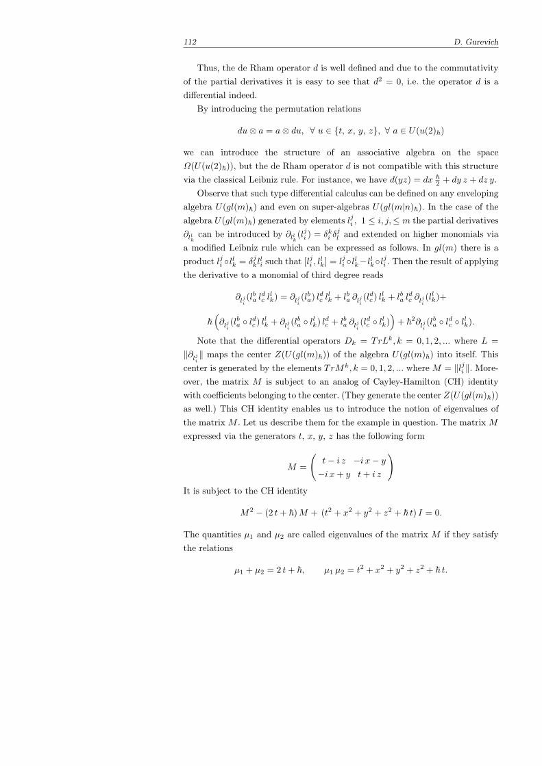
112 D. Gurevich
Thus, the de Rham operator d is well defined and due to the commutativityof the partial derivatives it is easy to see that d2 = 0, i.e. the operator d is adifferential indeed.
By introducing the permutation relations
du⊗ a = a⊗ du, ∀ u ∈ t, x, y, z, ∀ a ∈ U(u(2)~)
we can introduce the structure of an associative algebra on the spaceΩ(U(u(2)~)), but the de Rham operator d is not compatible with this structurevia the classical Leibniz rule. For instance, we have d(yz) = dx ~
2 + dy z + dz y.Observe that such type differential calculus can be defined on any enveloping
algebra U(gl(m)~) and even on super-algebras U(gl(m|n)~). In the case of thealgebra U(gl(m)~) generated by elements lji , 1 ≤ i, j,≤ m the partial derivatives∂llk can be introduced by ∂llk(l
ji ) = δki δ
jl and extended on higher monomials via
a modified Leibniz rule which can be expressed as follows. In gl(m) there is aproduct lji llk = δjkl
li such that [lji , l
lk] = lji llk−llkl
ji . Then the result of applying
the derivative to a monomial of third degree reads
∂lji(lba l
dc llk) = ∂lji
(lba) ldc llk + lba ∂lji
(ldc ) llk + lba l
dc ∂lji
(llk)+
~(∂lji
(lba ldc ) llk + ∂lji(lba llk) ldc + lba ∂lji
(ldc llk))+ ~2∂lji (l
ba ldc llk).
Note that the differential operators Dk = TrLk, k = 0, 1, 2, ... where L =
‖∂lji ‖ maps the center Z(U(gl(m)~)) of the algebra U(gl(m)~) into itself. Thiscenter is generated by the elements TrMk, k = 0, 1, 2, ... where M = ‖lji ‖. More-over, the matrix M is subject to an analog of Cayley-Hamilton (CH) identitywith coefficients belonging to the center. (They generate the center Z(U(gl(m)~))
as well.) This CH identity enables us to introduce the notion of eigenvalues ofthe matrix M . Let us describe them for the example in question. The matrix Mexpressed via the generators t, x, y, z has the following form
M =
(t− i z −i x− y−i x+ y t+ i z
)It is subject to the CH identity
M2 − (2 t+ ~)M + (t2 + x2 + y2 + z2 + ~ t) I = 0.
The quantities µ1 and µ2 are called eigenvalues of the matrix M if they satisfythe relations
µ1 + µ2 = 2 t+ ~, µ1 µ2 = t2 + x2 + y2 + z2 + ~ t.
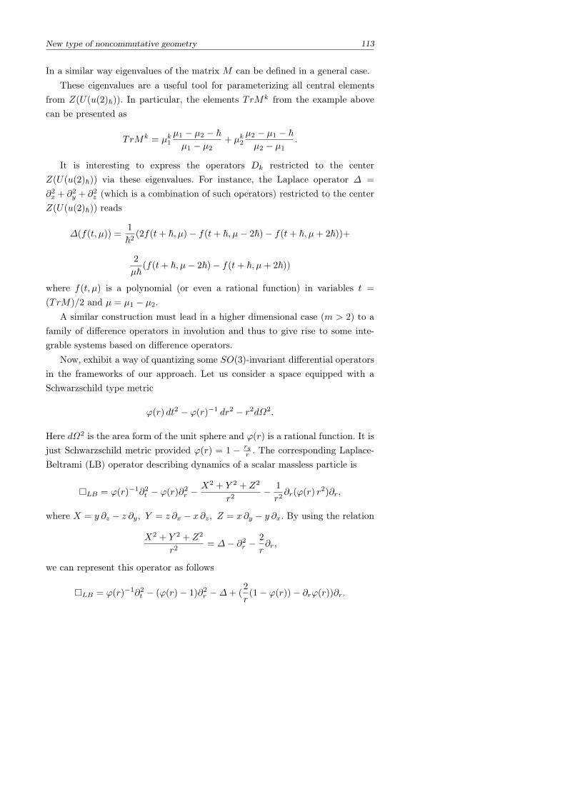
New type of noncommutative geometry 113
In a similar way eigenvalues of the matrix M can be defined in a general case.These eigenvalues are a useful tool for parameterizing all central elements
from Z(U(u(2)~)). In particular, the elements TrMk from the example abovecan be presented as
TrMk = µk1µ1 − µ2 − ~µ1 − µ2
+ µk2µ2 − µ1 − ~µ2 − µ1
.
It is interesting to express the operators Dk restricted to the centerZ(U(u(2)~)) via these eigenvalues. For instance, the Laplace operator ∆ =
∂2x + ∂2y + ∂2z (which is a combination of such operators) restricted to the centerZ(U(u(2)~)) reads
∆(f(t, µ)) =1
~2(2f(t+ ~, µ)− f(t+ ~, µ− 2~)− f(t+ ~, µ+ 2~))+
2
µ~(f(t+ ~, µ− 2~)− f(t+ ~, µ+ 2~))
where f(t, µ) is a polynomial (or even a rational function) in variables t =
(TrM)/2 and µ = µ1 − µ2.A similar construction must lead in a higher dimensional case (m > 2) to a
family of difference operators in involution and thus to give rise to some inte-grable systems based on difference operators.
Now, exhibit a way of quantizing some SO(3)-invariant differential operatorsin the frameworks of our approach. Let us consider a space equipped with aSchwarzschild type metric
ϕ(r) dt2 − ϕ(r)−1 dr2 − r2dΩ2.
Here dΩ2 is the area form of the unit sphere and ϕ(r) is a rational function. It isjust Schwarzschild metric provided ϕ(r) = 1 − rg
r . The corresponding Laplace-Beltrami (LB) operator describing dynamics of a scalar massless particle is
LB = ϕ(r)−1∂2t − ϕ(r)∂2r −X2 + Y 2 + Z2
r2− 1
r2∂r(ϕ(r) r
2)∂r,
where X = y ∂z − z ∂y, Y = z ∂x − x ∂z, Z = x ∂y − y ∂x. By using the relation
X2 + Y 2 + Z2
r2= ∆− ∂2r −
2
r∂r,
we can represent this operator as follows
LB = ϕ(r)−1∂2t − (ϕ(r)− 1)∂2r −∆+ (2
r(1− ϕ(r))− ∂rϕ(r))∂r.
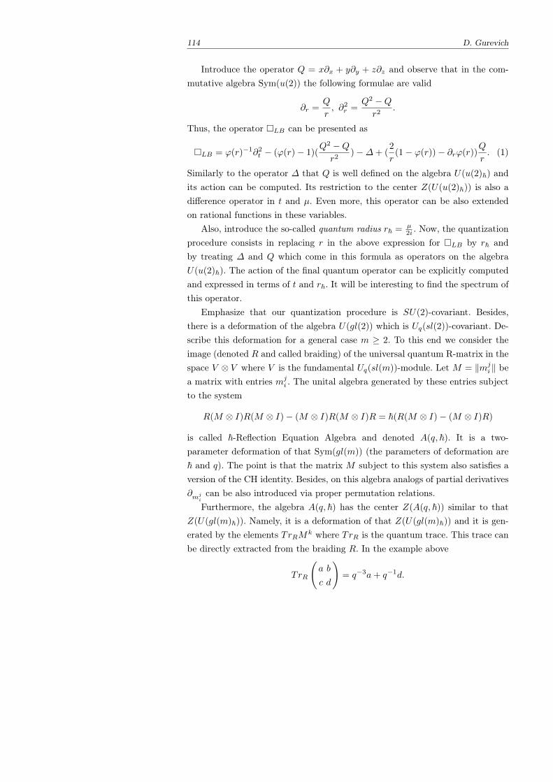
114 D. Gurevich
Introduce the operator Q = x∂x + y∂y + z∂z and observe that in the com-mutative algebra Sym(u(2)) the following formulae are valid
∂r =Q
r, ∂2r =
Q2 −Qr2
.
Thus, the operator LB can be presented as
LB = ϕ(r)−1∂2t − (ϕ(r)− 1)(Q2 −Qr2
)−∆+ (2
r(1− ϕ(r))− ∂rϕ(r))
Q
r. (1)
Similarly to the operator ∆ that Q is well defined on the algebra U(u(2)~) andits action can be computed. Its restriction to the center Z(U(u(2)~)) is also adifference operator in t and µ. Even more, this operator can be also extendedon rational functions in these variables.
Also, introduce the so-called quantum radius r~ = µ2i . Now, the quantization
procedure consists in replacing r in the above expression for LB by r~ andby treating ∆ and Q which come in this formula as operators on the algebraU(u(2)~). The action of the final quantum operator can be explicitly computedand expressed in terms of t and r~. It will be interesting to find the spectrum ofthis operator.
Emphasize that our quantization procedure is SU(2)-covariant. Besides,there is a deformation of the algebra U(gl(2)) which is Uq(sl(2))-covariant. De-scribe this deformation for a general case m ≥ 2. To this end we consider theimage (denoted R and called braiding) of the universal quantum R-matrix in thespace V ⊗ V where V is the fundamental Uq(sl(m))-module. Let M = ‖mj
i‖ bea matrix with entries mj
i . The unital algebra generated by these entries subjectto the system
R(M ⊗ I)R(M ⊗ I)− (M ⊗ I)R(M ⊗ I)R = ~(R(M ⊗ I)− (M ⊗ I)R)
is called ~-Reflection Equation Algebra and denoted A(q, ~). It is a two-parameter deformation of that Sym(gl(m)) (the parameters of deformation are~ and q). The point is that the matrix M subject to this system also satisfies aversion of the CH identity. Besides, on this algebra analogs of partial derivatives∂mji
can be also introduced via proper permutation relations.Furthermore, the algebra A(q, ~) has the center Z(A(q, ~)) similar to that
Z(U(gl(m)~)). Namely, it is a deformation of that Z(U(gl(m)~)) and it is gen-erated by the elements TrRMk where TrR is the quantum trace. This trace canbe directly extracted from the braiding R. In the example above
TrR
(a b
c d
)= q−3a+ q−1d.
All these properties enable us to generalize a large part of the above constructionsto this algebra.
We want to complete this note with a historical remark exhibiting a role ofthe ~-Reflection Equation Algebra in constructing our differential calculus on thealgebras U(gl(m)~) (or U(u(m)~)). In a number of papers [W,IP,FP] a version ofdifferential calculus was constructed on a pseudogroup (in fact an RTT algebra).In [GPS1] we suggested a generalization of this construction by replacing thisalgebra by other Quantum Matrix Algebras (QMA). In a particular case, therole of such QMA is played by a ~-Reflection Equation Algebra (may be withh = 0). Thus, in [GPS2] we introduced a braided version of Weyl algebra whichin the limit q → 1 given rise to differential calculus presented above.
The most amazing consequence of this calculus consists in the following.Though it is defined on a Noncommutative algebra but the final operators comingin the above dynamical models are difference ones. Thus, these operators canbe defined on a lattice and consequently the space-time can be considered asdiscrete. It will be interesting to study physical consequences of this conclusion.
References
[FP] Faddeev L., Pyatov P. The Differential calculus on quantum linear groups, Amer. Math.Soc. Transl. Ser. 2, 175.
[GPS1] Gurevich D., Pyatov P., Saponov P. Braided differential operators on quantum alge-bras, J. of Geometry and Physics 61 (2011), 1485–1501.
[GPS2] Gurevich D., Pyatov P., Saponov P. Braided Weyl algebras and differential calculuson U(u(2)), J. of Geometry and Physics 62 (2012), 1175–1188.
[IP] Isaev A., Pyatov P. Covariant differential calculus complexes on quantum linear groups,J.Phys. A 28 (1995) 8, 2227–2246.
[W] Woronowicz S. Differential Calculus on Compact Matrix Pseudogroups (Quantumgroups), CMP 122 (1989), 125–170.
Dimitri GurevichValenciennes UniversityE-mail: [email protected]
Tropical and Idempotent Mathematics. Moscow, Russia, August 26–31, 2012
Bounds for tropical, determinantal and Gondran-Minoux ranks
Alexander E. GutermanYaroslav N. Shitov
1 Introduction
Definition 1 The set of real numbers with the additional element −∞ is calledthe max-algebra (it is sometimes also called max-plus algebra or tropical algebra),denoted Rmax, if the operations of addition, ⊕, and multiplication, ⊗, on this setare defined in the following way: a ⊕ b = maxa, b, a ⊗ b = a + b, correspond-ingly. Here neutral element with respect to addition is −∞ and neutral elementwith respect to multiplication is 0. Rmax with these operations is an algebraicstructure, called a semiring .
For the purpose of this paper it is more convenient to use the exponentialmodel of the max-algebra which is defined below and directly obtained by ap-plying the exponent function to the ordinary model introduced above.
Definition 2 The max-algebra R is the set of non-negative real numbers withthe operations of addition and multiplication defined by a ⊕ b = maxa, b,a ⊗ b = a · b, correspondingly. Here neutral element with respect to addition is0 ∈ R and neutral element with respect to multiplication is 1 ∈ R.
Definition 3 The binary Boolean semiring B is the set 0, 1 with the oper-ations of addition and multiplication defined by a ⊕ b = maxa, b, a ⊗ b =
mina, b, correspondingly.
We consider matrices over B and R. The set of m× n matrices with entriesfrom a set S is denoted byMm×n(S) andMn(S) =Mn×n(S). By O we denote
Bounds for tropical, determinantal and Gondran-Minoux ranks 117
a zero matrix, i.e., all elements of O are equal to 0. By A[r1, . . . , rk] we denotethe matrix formed by the rows of the matrix A with the indexes r1, . . . , rk. ByA[r1, . . . , rk|c1, . . . , cm] we denote the submatrix of A located on the intersec-tion of the rows with the indexes r1, . . . , rk and the columns with the indexesc1, . . . , cm. By aij we denote the entry in the ith row and jth column of A.
There are many different approaches to define the notion of rank for matri-ces over max-algebras and binary Boolean semirings, see for example [1] for thedetailed and self-contained information on this subject. In this paper we con-sider the notions of tropical rank (see [1, 3,7]), determinantal rank (see [1]) andGondran-Minoux rank (see [1, 4, 5]). Let us start with the exact definitions ofthese notions.
Definition 4 The tropical permanent of an n×nmatrix A= (aij) with elementsfrom B or R is the following function
perm(A) = maxσ∈Sn
a1,σ(1) · · · an,σ(n), (1)
where Sn denotes the symmetric group on 1, . . . , n.
Definition 5 Let S = B or R. A matrix A ∈Mn(S) is called tropically singularif n = 1 and perm(A) = 0 or if the maximum in the expression (1) is achievedat least on two different permutations in Sn. A matrix that is not tropicallysingular is called tropically nonsingular.
Remark 1 In particular, if n ≥ 2 and perm(A) = 0, then for any σ ∈ Sn it holdsthat a1,σ(1) . . . an,σ(n) = 0, hence A is tropically singular.
Definition 6 Let S = B or R. The tropical rank trop(A) of a matrix A ∈Mn(S)is the maximal size of a tropically nonsingular square submatrix of A. By thedefinition trop(O) = 0.
Definition 7 Let S = B or R and let A= (aij) ∈Mn(S). Elements
‖A‖+ = maxτ∈An
a1,τ(1) . . . an,τ(n), ‖A‖− = maxϕ∈Sn\An
a1,ϕ(1) . . . an,ϕ(n) ∈ S
are called respectively the positive determinant and the negative determinant ofA. Here An ⊂ Sn denotes the subgroup of even permutations.
Definition 8 Let S = B or R. A matrix A ∈ Mn(S) is called d-nonsingular, if‖A‖+ 6= ‖A‖−. In the case ‖A‖+ = ‖A‖−, the matrix A is called d-singular.
Definition 9 Let S = B or R, A ∈Mn(S). The determinantal rank d(A) is themaximal size of d-nonsingular square submatrix of A. By the definition d(O) = 0.
118 A. E. Guterman, Ya. N. Shitov
Definition 10 Let S = B or R. A set a1, . . . , an of vectors from Sm, ai =
(ai1, . . . , aim)t, is called Gondran-Minoux dependent (or shortly, GM-dependent)
if there are subsets I, J ⊂ 1, . . . , n, I ∩ J = ∅, I ∪ J 6= ∅ and elementsλ1, . . . , λn ∈ S, λt 6= 0, t ∈ I ∪ J , such that for all k ∈ 1, . . . ,m it holds that
maxi∈Iλiaik = max
j∈Jλjajk. (2)
In the case, a set of vectors is not GM-dependent, then it is called GM-independent.
Definition 11 The maximal number of vectors in all GM-independent sub-sets of the set a1, . . . , an is called Gondran-Minoux rank (GM-rank) of the seta1, . . . , an and is denoted by GM(a1, . . . , an).
Definition 12 Let S = B or R, A ∈ Mn(S). GM-rank of the set of rows of Ais called row GM-rank of A and is denoted by GMr(A). GM-rank of the set ofcolumns of A is called column GM-rank of A and is denoted by GMc(A).
Remark 2 Note that row GM-rank and column GM-rank can be different, fordetails see the work of the second author [13] or Example 1 in this paper. Belowby GM-rank we mean row GM-rank.
The notion of GM-independence is related to the notion of L-matrices, whichcan be found in [9, 12].
Definition 13 Let A ∈Mn(R) be a real matrix, c1, . . . , cn be its columns. It issaid that A is not an L-matrix if there are subsets I, J ⊂ 1, . . . , n, I ∩ J = ∅,I ∪J 6= ∅, such that every nonzero row of the matrix A′ formed by the columnsci,−cji∈I,j∈J contains both positive and negative elements. Otherwise A iscalled an L-matrix .
Remark 3 From Definitions 10 and 13 we have that a 0-1matrix A is an L-matrixiff the columns of A are GM-independent over B.
The properties of GM-independence and d-nonsingularity are equivalent:
Fact 1 [4, Chapter 5, Corollary 3.4.3] Let S = B or R. The following conditionsare equivalent for A ∈Mn(S):
1) The rows (columns) of A are GM-dependent;2) ‖A‖+ = ‖A‖−.
Remark 4 From Remark 3 and Fact 1 it follows that a square 0-1 matrix A isan L-matrix iff A is d-nonsingular.
Bounds for tropical, determinantal and Gondran-Minoux ranks 119
In this paper we introduce the notion of the tropical matrix pattern, whichprovides a powerful tool to investigate tropical matrices. The above approach isthen illustrated by the application to the study of the properties of the Gondran-Minoux rank function. Our main result states that up to a multiplication ofmatrix rows by non-zero constants the Gondran-Minoux independence of thematrix rows and that of the rows of its tropical pattern are equivalent.
As a consequence of our main result we obtain that the tropical rank, trop(A),and the determinantal rank, d(A), of tropical matrices satisfy the following in-equalities: trop(A) >
√GMr(A), d(A) >
√GMr(A), trop(A) > d(A)+2
3 . Asan important corollary of this result we obtain that if one of these functionsis bounded then the other two are also bounded unlike the situation with thefactor and Kapranov ranks.
The purpose of this note is to state our result. The detailed proofs will beavailable soon in [6].
2 Tropical pattern technique and its applications
We first introduce the notion of the tropical pattern of a matrix for A ∈Mn×m(R). It is shown that up to the multiplication of rows of a matrix bypositive numbers, GM-dependence of rows of any matrix is equivalent to GM-dependence of rows of its tropical pattern. This enables us to generalize severalresults proved for matrices over B to the matrices over max-algebras.
Next we present a number of applications of the pattern technique. Some gen-eral properties of GM-rank, determinantal rank and tropical rank of matricesover R are investigated. We provide minimal (with respect to the size of matri-ces) examples where these functions are different. Also we prove the followinginequalities trop(A) >
√GMr(A), trop(A) > d(A)+2
3 , d(A) >√GMr(A) for
matrices with coefficients from B and R.
2.1 Tropical pattern and GM-independence
Main Definition 1 The tropical pattern of a matrix A = (aij) ∈ Mn×m(R)is the matrix B = (bij) ∈Mn×m(B) defined by
buv =
1 if auv = maxni=1aiv > 0,
0 if either auv = 0 or auv < maxni=1aiv.
The tropical pattern of the matrix A is denoted by P(A).
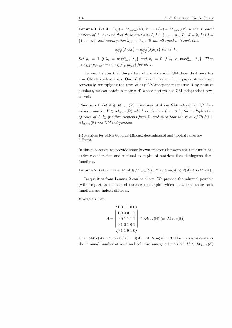
120 A. E. Guterman, Ya. N. Shitov
Lemma 1 Let A= (aij) ∈ Mn×m(R), W = P(A) ∈ Mn×m(B) be the tropicalpattern of A. Assume that there exist sets I, J ⊂ 1, . . . , n, I ∩ J = ∅, I ∪ J =
1, . . . , n, and nonnegative λ1, . . . , λn ∈ R not all equal to 0 such that
maxi∈Iλiaik = max
j∈Jλjajk for all k.
Set µt = 1 if λt = maxnu=1λu and µt = 0 if λt < maxnu=1λu. Thenmaxi∈Iµiwik = maxj∈Jµjwjk for all k.
Lemma 1 states that the pattern of a matrix with GM-dependent rows hasalso GM-dependent rows. One of the main results of our paper states that,conversely, multiplying the rows of any GM-independent matrix A by positivenumbers, we can obtain a matrix A′ whose pattern has GM-independent rowsas well:
Theorem 1 Let A ∈ Mn×m(R). The rows of A are GM-independent iff thereexists a matrix A′ ∈ Mn×m(R) which is obtained from A by the multiplicationof rows of A by positive elements from R and such that the rows of P(A′) ∈Mn×m(B) are GM-independent.
2.2 Matrices for which Gondran-Minoux, determinantal and tropical ranks aredifferent
In this subsection we provide some known relations between the rank functionsunder consideration and minimal examples of matrices that distinguish thesefunctions.
Lemma 2 Let S = B or R, A ∈Mn×n(S). Then trop(A) 6 d(A) 6 GMr(A).
Inequalities from Lemma 2 can be sharp. We provide the minimal possible(with respect to the size of matrices) examples which show that these rankfunctions are indeed different.
Example 1 Let
A =
1 0 1 1 0 0
1 0 0 0 1 1
0 0 1 1 1 1
0 1 0 1 0 1
0 1 1 0 1 0
∈M5×6(B) (orM5×6(R)).
Then GMr(A) = 5, GMc(A) = d(A) = 4, trop(A) = 3. The matrix A containsthe minimal number of rows and columns among all matrices M ∈ Mn×m(S)
Bounds for tropical, determinantal and Gondran-Minoux ranks 121
such that GMr(M) > d(M) and among all matrices N ∈ Mn×m(S) such thatGMr(N) > GMc(N).
Example 2 Let
B =
0 1 1
1 0 1
1 1 0
∈M3×3(B) (orM3×3(R)).
Then GMr(B) = d(B) = 3, trop(B) = 2. The matrix B contains the min-imal possible number of columns among all matrices M ∈ Mn×m(S) suchthat GMr(M) > trop(M) and among all matrices N ∈ Mn×m(S) such thatd(N) > trop(N).
2.3 Inequalities for matrix rank functions over B
In this section we state the following inequalities: trop(A) >√GMr(A),
trop(A) > d(A)+23 , d(A) >
√GMr(A) for any A ∈Mn×m(B).
Theorem 2 Let the rows of A ∈ Mn×m(B) be GM-independent. Thentrop(A) >
√n.
Theorem 3 Let A ∈Mn×m(B). Then trop(A) >√GMr(A).
The next inequality which connects GM- and determinantal ranks for matri-ces over B, is a direct consequence of Theorem 3.
Corollary 1 Let A ∈Mn×m(B). Then d(A) >√GMr(A).
Now we are going to formulate the inequality relating determinantal andtropical ranks for matrices over B.
Lemma 3 Let A ∈Mn×n(B), and elements p1, . . . , pt ∈ 1, . . . , n be different.Assume that for any q1, . . . , qt ∈ 1, . . . , n, we have that
‖A[p1, . . . , pt|q1, . . . , qt]‖+ = ‖A[p1, . . . , pt|q1, . . . , qt]‖−.
Then ‖A‖+ = ‖A‖−.
Theorem 4 Let A ∈ Mn×n(B) be such that ‖A‖+ 6= ‖A‖−. Then trop(A) >n+23 .
Now we are ready to state the inequality relating determinantal and tropicalranks of matrices over B.
Theorem 5 Let A ∈Mn×m(B). Then trop(A) > d(A)+23 .
2.4 Matrices over R
In this subsection, using the characterization of the GM-rank of matrices via theGM-ranks of tropical patterns, we generalize the main results from the previoussubsection to R.
Theorem 6 Let A ∈ Mn×m(R), W = P(A) ∈ Mn×m(B). Then trop(A) >
trop(W ).
Theorem 7 Let A ∈Mn×m(R). Then trop(A) >√GMr(A).
Theorem 8 Let A ∈Mn×m(R). Then trop(A) > d(A)+23 .
Corollary 2 Let A ∈Mn×m(R). Then d(A) >√GMr(A).
The following consequence from the obtained results is very important. Inparticular it underlines the difference of the functions under consideration withthe factor and Kapranov ranks, cf. [1–3,8].
Corollary 3 Let one of the functions trop(A), d(A), GMr(A) is bounded. Thenthe other two are also bounded.
References
1. M. Akian, S. Gaubert, A. Guterman. Linear independence over tropical semirings andbeyond // Contemporary Mathematics, AMS, 495(2009) 1–38.
2. L. B. Beasley, T. J. Laffey. Real rank versus nonnegative rank // Linear Algebra and itsApplications, 431(12)(2009), 2330-2335.
3. M. Develin, F. Santos, B. Sturmfels. On the rank of a tropical matrix, in Discrete andComputational Geometry (E. Goodman, J. Pach and E. Welzl, eds.), MSRI Publications,Cambridge Univ., Press, 2005.
4. M. Gondran, M. Minoux. Graphs, Dioids and Semirings: New Models and Algorithms,Springer Science+Business Media, LLC, 2008.
5. M. Gondran, M. Minoux. L’independance lineaire dans les dioides, E.D.F. — Bulletin dela Direction des Etudies et Recherches, Serie C — Mathematiques, Informatique 1(1978),67–90.
6. A. Guterman, Ya. Shitov. Tropical patterns of matrices and the Gondran–Minoux rankfunction // Linear Algebra and its Applications, accepted.
7. K. H. Kim, N. F. Roush. Kapranov rank vs. tropical rank // Proc. Amer. Math. Soc.,134(9)(2006), 2487–2494.
8. K. H. Kim, N. F. Roush. Factorization of polynomials in one variable over the tropicalsemiring // arxiv:math.CO/0501167.
9. V. Klee, R. Ladner, and R. Manber. Sign-solvability revisited // Linear Algebra Appl.,59(1984), 131–158.
10. P. L. Poplin, R. E. Hartwig. Determinantal identities over commutative semirings //Linear Algebra Appl., 387(2004), 99–132.
11. Ya. Shitov. Inequalities for Gondran-Minoux rank and idempotent semirings // LinearAlgebra Appl., doi:10.1016/j.laa.2010.09.032 (2010).
12. C. Thomassen. Sign-nonsingular matrices and even cycles in directed graphs // LinearAlgebra Appl. 75(1986), 27–41.
13. Ya. Shitov. Minimal example of a matrix which distinguishes GM- and d- ranks over max-algebras // Fundamental and Applied Mathematics, 14(4)(2008), 231–268 [in Russian].

Alexander E. GutermanFaculty of Algebra, Department of Mathematics and Mechanics, Moscow StateUniversityE-mail: [email protected] N. ShitovFaculty of Algebra, Department of Mathematics and Mechanics, Moscow StateUniversityE-mail: [email protected]
Tropical and Idempotent Mathematics. Moscow, Russia, August 26–31, 2012
Singularities for tropical limit/dequantization
B. Kh. Kirshtein
To keep in mind some engineering applications, it is important to be able toestimate the proximity of solutions of equations or systems of equations to theirsingular values.
A natural way to do this is a transfer to the so-called tropicallimit/dequantization and comparison of properties of real and complex solu-tions of the original equations with properties of tropical solutions of equationsafter the transfer to the tropical limit.
For instance, if we consider real and complex tropical roots in the senseof hyperfields theory [1], then appearance of singularities in the process of thetransition to the tropical limit can be found if some of complex roots becomereal tropical after the transition to the tropical limit. In this way we can detectsingularities working with tropical solutions before their real appearance in realor in complex settings.
We discuss two examples of this type.
In the first one we consider a numerical method which allows us to comparethe number of all real solutions of polynomials in one variable with real coef-ficients and the number of all tropical real solutions of these polynomials afterthe transfer to the tropical limit.
In the second example we consider some systems of polynomial equationsarising in electrical power industry. In this case we give a simple test for ap-pearance of singularities after the transfer to the tropical limit in terms of somespanning trees of graphs of electrical networks. We can use this test as a modelfor predictions of the instability of electrical power networks.

This work is supported by the grant RFBR 12-01-00886-a and the jointRFBR-CNRS grant 11-01–93106-a
References
1. O.Viro, Hyperfields in tropical geometry I. Hyperfields and dequntization, E-printarXiv:math.AG/1006.3034v2.
B. Kh. KirshteinScientific and Production Company “Del’fin–Informatika,” Moscow, RussiaE-mail: [email protected]
Tropical and Idempotent Mathematics. Moscow, Russia, August 26–31, 2012
On Maslov’s quantization of thermodynamics
V. N. Kolokoltsov
The program of the tunnel quantization of thermodynamics was put forwardby V. P. Maslov some 20 years ago, as a possible link of Idempotent (Tropi-cal) mathematics and statistical physics. Many papers by Maslov and his col-laborators have been published since then. Very beautiful underlying ideas arescattered among technical results. Our objective is to present a personal viewon these ideas, or better to say some bunch of these ideas related to two majorpoints: quantization of critical exponents and fractional dimensions. We aim togive a clear glimps of the picture for nonexperts starting from the basics, explain-ing the main idealogical link number theory–economics–physics and indicatingthe perspectives.
V. N. KolokoltsovThe University of Warwick, [email protected]
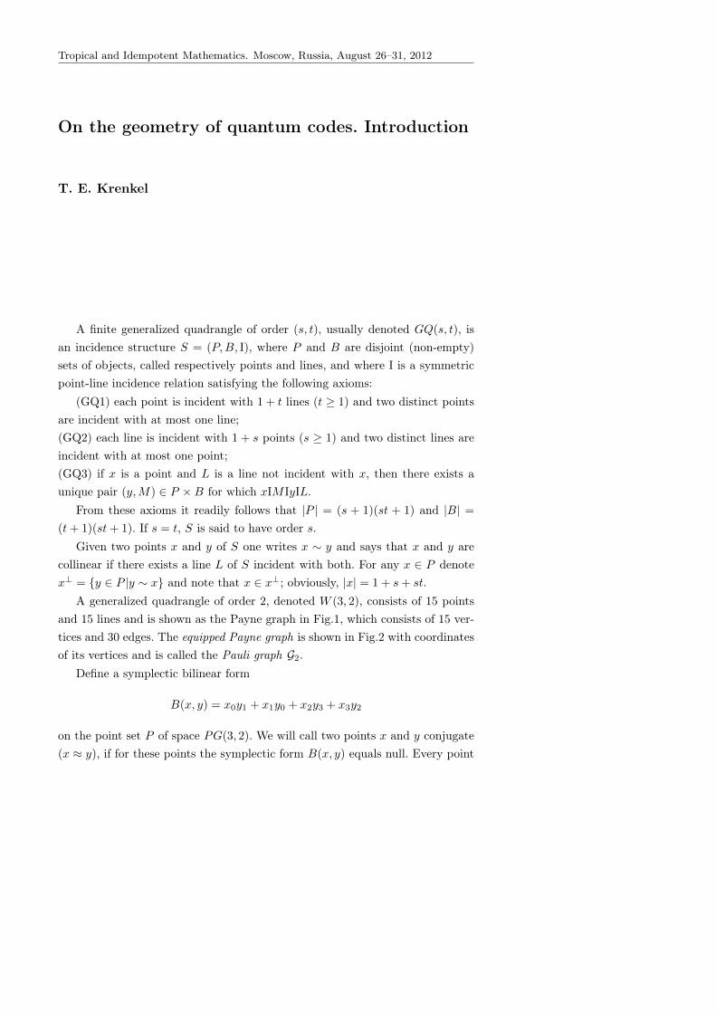
Tropical and Idempotent Mathematics. Moscow, Russia, August 26–31, 2012
On the geometry of quantum codes. Introduction
T. E. Krenkel
A finite generalized quadrangle of order (s, t), usually denoted GQ(s, t), isan incidence structure S = (P,B, I), where P and B are disjoint (non-empty)sets of objects, called respectively points and lines, and where I is a symmetricpoint-line incidence relation satisfying the following axioms:
(GQ1) each point is incident with 1 + t lines (t ≥ 1) and two distinct pointsare incident with at most one line;(GQ2) each line is incident with 1 + s points (s ≥ 1) and two distinct lines areincident with at most one point;(GQ3) if x is a point and L is a line not incident with x, then there exists aunique pair (y,M) ∈ P ×B for which xIM IyIL.
From these axioms it readily follows that |P | = (s + 1)(st + 1) and |B| =(t+ 1)(st+ 1). If s = t, S is said to have order s.
Given two points x and y of S one writes x ∼ y and says that x and y arecollinear if there exists a line L of S incident with both. For any x ∈ P denotex⊥ = y ∈ P |y ∼ x and note that x ∈ x⊥; obviously, |x| = 1 + s+ st.
A generalized quadrangle of order 2, denoted W (3, 2), consists of 15 pointsand 15 lines and is shown as the Payne graph in Fig.1, which consists of 15 ver-tices and 30 edges. The equipped Payne graph is shown in Fig.2 with coordinatesof its vertices and is called the Pauli graph G2.
Define a symplectic bilinear form
B(x, y) = x0y1 + x1y0 + x2y3 + x3y2
on the point set P of space PG(3, 2). We will call two points x and y conjugate(x ≈ y), if for these points the symplectic form B(x, y) equals null. Every point
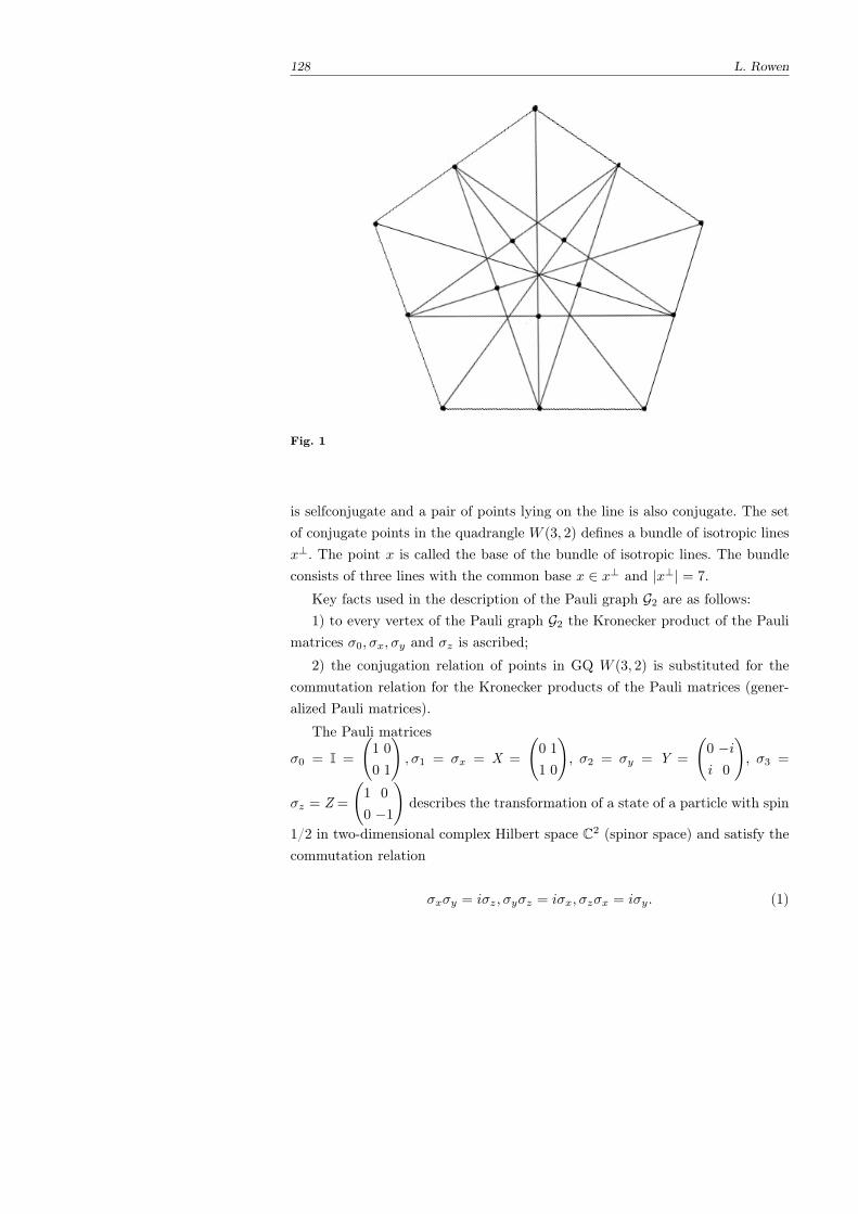
128 L. Rowen
Fig. 1
is selfconjugate and a pair of points lying on the line is also conjugate. The setof conjugate points in the quadrangle W (3, 2) defines a bundle of isotropic linesx⊥. The point x is called the base of the bundle of isotropic lines. The bundleconsists of three lines with the common base x ∈ x⊥ and |x⊥| = 7.
Key facts used in the description of the Pauli graph G2 are as follows:1) to every vertex of the Pauli graph G2 the Kronecker product of the Pauli
matrices σ0, σx, σy and σz is ascribed;
2) the conjugation relation of points in GQ W (3, 2) is substituted for thecommutation relation for the Kronecker products of the Pauli matrices (gener-alized Pauli matrices).
The Pauli matrices
σ0 = I =
(1 0
0 1
), σ1 = σx = X =
(0 1
1 0
), σ2 = σy = Y =
(0 −ii 0
), σ3 =
σz = Z =
(1 0
0 −1
)describes the transformation of a state of a particle with spin
1/2 in two-dimensional complex Hilbert space C2 (spinor space) and satisfy thecommutation relation
σxσy = iσz, σyσz = iσx, σzσx = iσy. (1)
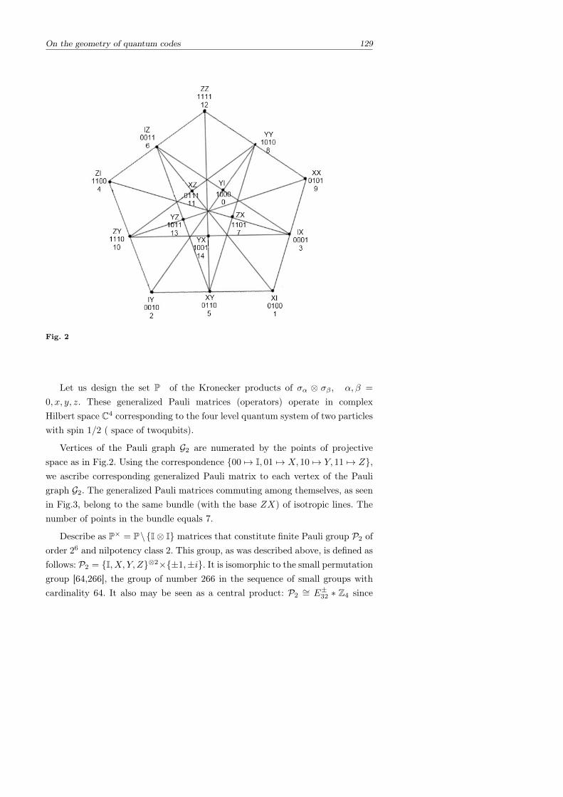
On the geometry of quantum codes 129
Fig. 2
Let us design the set P of the Kronecker products of σα ⊗ σβ , α, β =
0, x, y, z. These generalized Pauli matrices (operators) operate in complexHilbert space C4 corresponding to the four level quantum system of two particleswith spin 1/2 ( space of twoqubits).
Vertices of the Pauli graph G2 are numerated by the points of projectivespace as in Fig.2. Using the correspondence 00 7→ I, 01 7→ X, 10 7→ Y, 11 7→ Z,we ascribe corresponding generalized Pauli matrix to each vertex of the Pauligraph G2. The generalized Pauli matrices commuting among themselves, as seenin Fig.3, belong to the same bundle (with the base ZX) of isotropic lines. Thenumber of points in the bundle equals 7.
Describe as P× = P\I⊗ I matrices that constitute finite Pauli group P2 oforder 26 and nilpotency class 2. This group, as was described above, is defined asfollows: P2 = I, X, Y, Z⊗2×±1,±i. It is isomorphic to the small permutationgroup [64,266], the group of number 266 in the sequence of small groups withcardinality 64. It also may be seen as a central product: P2
∼= E±32 ∗ Z4 since
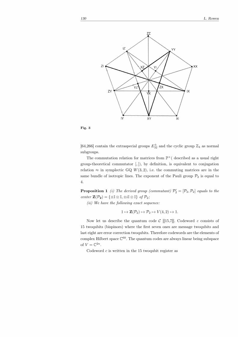
130 L. Rowen
Fig. 3
[64,266] contain the extraspecial groups E±32 and the cyclic group Z4 as normalsubgroups.
The commutation relation for matrices from P×( described as a usual rightgroup-theoretical commutator [, ]), by definition, is equivalent to conjugationrelation ≈ in symplectic GQ W (3, 2), i.e. the commuting matrices are in thesame bundle of isotropic lines. The exponent of the Pauli group P2 is equal to4.
Proposition 1 (i) The derived group (commutant) P ′2 = [P2,P2] equals to thecenter Z(P2) = ±I⊗ I,±iI⊗ I of P2;
(ii) We have the following exact sequence:
1 7→ Z(P2) 7→ P2 7→ V (4, 2) 7→ 1.
Now let us describe the quantum code C [[15,7]]. Codeword c consists of15 twoqubits (bispinors) where the first seven ones are message twoqubits andlast eight are error correction twoqubits. Therefore codewords are the elements ofcomplex Hilbert space C60. The quantum codes are always linear being subspaceof V = C2n.
Codeword c is written in the 15 twoqubit register as
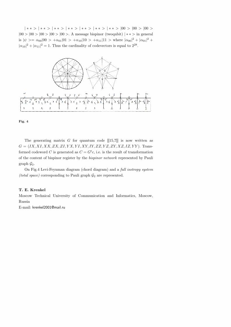
| ∗ ∗ > | ∗ ∗ > | ∗ ∗ > | ∗ ∗ > | ∗ ∗ > | ∗ ∗ > | ∗ ∗ > |00 > |00 > |00 >
|00 > |00 > |00 > |00 > |00 >. A message bispinor (twoqubit) | ∗ ∗ > in generalis |ψ >= α00|00 > +α01|01 > +α10|10 > +α11|11 > where |α00|2 + |α01|2 +
|α10|2 + |α11|2 = 1. Thus the cardinality of codevectors is equal to 228.
Fig. 4
The generating matrix G for quantum code [[15,7]] is now written asG = (IX,XI,XX,ZX,ZI, Y X, Y I,XY, IY, ZZ, Y Z,ZY,XZ, IZ, Y Y ). Trans-formed codeword C is generated as C = Gtc, i.e. is the result of transformationof the content of bispinor register by the bispinor network represented by Pauligraph G2.
On Fig.4 Levi-Feynman diagram (chord diagram) and a full isotropy system(total space) corresponding to Pauli graph G2 are represented.
T. E. KrenkelMoscow Technical University of Communication and Informatics, Moscow,RussiaE-mail: [email protected]
Tropical and Idempotent Mathematics. Moscow, Russia, August 26–31, 2012
Solution to an extremal problem in tropical math-ematics
Nikolai Krivulin
1 Introduction
Methods and computational procedures for solving multidimensional extremalproblems are among the topical lines of investigation in the linear tropical (idem-potent) algebra [1–7]. We consider the problems of minimizing linear or nonlin-ear functionals defined on finite-dimensional semimodules over idempotent semi-fields, with possible additional constraints imposed on the feasible solution setin the form of linear equations and inequalities. The problems under study inthe area include idempotent analogues of linear programming problems [7,8] aswell as their extensions with nonlinear objective functions [9–14]. In addition,there exist solutions to some problems where both the objective function andconstraints appear to be nonlinear [15,16].
Many extremal problems under consideration are stated and solved in termsof specific semifields (see, e.g., [7–9] which concentrate on the classical semifieldRmax,+). Other results [10–14] offer solutions in more general setting which takeRmax,+ as a particular case. In some cases, solutions to extremal problems aregiven in the form of an iterative computational algorithm that produces a so-lution if any, or indicate that there is no solution otherwise [7–9]. Some otherproblems allow one to obtain a closed-form solution as in [10–14]. It is worthnoting that the existing approaches normally produce one or more particularsolutions provided that they exist, rather than give a comprehensive completesolution to the problems.
Solution to an extremal problem in tropical mathematics 133
In this paper, we consider a multidimensional extremal problem that is ageneralization of problems examined in [10,11,14]. Based on the implementationof methods and techniques developed in [11,12,18], we obtain all the solutions ofthe problem in an explicit and closed form that is appropriate for both fartheranalysis and development of computation procedures.
2 Preliminary Definitions and Results
We start with a brief overview of basic concepts, notations, and results from[11, 12, 18] that underlie the main findings presented in the paper. Additionalrelated details and thorough consideration can be found in [1–7].
2.1 Idempotent Semifield
Let X be a set equipped with two operations, addition ⊕ and multiplication⊗, with their respective neutral elements, zero 0 and identity 1. We assume(X,0,1,⊕,⊗) to be a commutative semiring where the addition is idempotentand the multiplication is invertible. Since the set of nonzero elements X+ =
X \ 0 forms a group under multiplication, such semiring is usually referred toas an idempotent semifield.
The power notation with integer exponent is routinely defined in the semifieldto represent iterated multiplication. Moreover, the integer power is assumed tobe extendable to rational exponents, and so the semifield is taken to be radicable.
From here on, as is customary in conventional algebra, we drop the multipli-cation sign ⊗. The power notation is used in the sense of idempotent algebra.
The idempotent addition naturally induces a partial order in the semifield.We suppose that the partial order can be completed into a linear order and thusconsider the semifield as totally ordered. In what follows, the relation signs arethought of as referring to this linear order.
Examples of totally ordered idempotent radicable semifields include
Rmax,+ = (R ∪ −∞,−∞, 0,max,+), Rmin,+ = (R ∪ +∞,+∞, 0,min,+),
Rmax,× = (R+ ∪ 0, 0, 1,max,×), Rmin,× = (R+ ∪ +∞,+∞, 1,min,×),
where R is the set of real numbers, R+ = x ∈ R|x > 0.
134 N. Krivulin
2.2 Idempotent Semimodule
Consider the Cartesian power Xn with its elements represented as column vec-tors. A vector with all zero entries is the zero vector denoted by 0. Vector addition⊕ and multiplication by scalars ⊗ are routinely defined componentwise on thebasis of the scalar addition and multiplication on X.
The set Xn with the above operations is an idempotent semimodule over X.A vector is called regular if it has no zero entries. The set of all regular vectors
of order n over X+ is denoted by Xn+.For any nonzero column vector x = (xi) ∈ Xn, we introduce a row vector
x− = (x−i ), where x−i = x−1i if xi 6= 0, and x−i = 0 otherwise, i = 1, . . . , n.
2.3 Matrix Algebra
For conforming matrices with elements in X, matrix addition and multiplicationtogether with multiplication by scalars are performed according to the standardrules applied to the scalar operations defined in X.
A matrix with all zero entries is the zero matrix which is denoted by 0.Consider the set of square matrices Xn×n. Any matrix that has all off-
diagonal entries equal to 0 is called diagonal. The diagonal matrix with alldiagonal entries equal to 1 is the identity matrix denoted by I. With respectto matrix addition and multiplication, the set Xn×n is an idempotent semiringwith identity.
For every matrix A = (aij), its trace is given by
trA =
n⊕i=1
aii.
A matrix is reducible if it can be put in a block-triangular (normal) formby simultaneous permutations of rows and columns. Otherwise the matrix isirreducible.
The normal form of a matrix A ∈ Xn×n is given by
A =
A11 0 . . . 0
A21 A22 0...
.... . .
As1 As2 . . . Ass
, (2)
where Aii is an irreducible or zero matrix of order ni, Aij is an arbitrary matrixof size ni × nj for all j < i with i = 1, . . . , s, and n1 + · · ·+ ns = n.
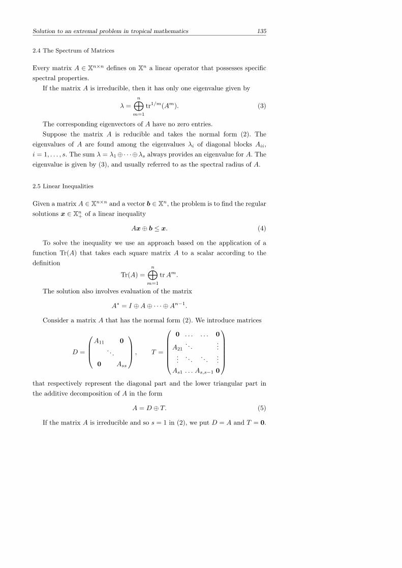
Solution to an extremal problem in tropical mathematics 135
2.4 The Spectrum of Matrices
Every matrix A ∈ Xn×n defines on Xn a linear operator that possesses specificspectral properties.
If the matrix A is irreducible, then it has only one eigenvalue given by
λ =
n⊕m=1
tr1/m(Am). (3)
The corresponding eigenvectors of A have no zero entries.Suppose the matrix A is reducible and takes the normal form (2). The
eigenvalues of A are found among the eigenvalues λi of diagonal blocks Aii,i = 1, . . . , s. The sum λ = λ1⊕· · ·⊕λs always provides an eigenvalue for A. Theeigenvalue is given by (3), and usually referred to as the spectral radius of A.
2.5 Linear Inequalities
Given a matrix A ∈ Xn×n and a vector b ∈ Xn, the problem is to find the regularsolutions x ∈ Xn+ of a linear inequality
Ax⊕ b ≤ x. (4)
To solve the inequality we use an approach based on the application of afunction Tr(A) that takes each square matrix A to a scalar according to thedefinition
Tr(A) =
n⊕m=1
trAm.
The solution also involves evaluation of the matrix
A∗ = I ⊕A⊕ · · · ⊕An−1.
Consider a matrix A that has the normal form (2). We introduce matrices
D =
A11 0
. . .
0 Ass
, T =
0 . . . . . . 0
A21. . .
......
. . . . . ....
As1 . . . As,s−1 0
that respectively represent the diagonal part and the lower triangular part inthe additive decomposition of A in the form
A = D ⊕ T. (5)
If the matrix A is irreducible and so s = 1 in (2), we put D = A and T = 0.
136 N. Krivulin
Lemma 1 Let x be the regular solution of inequality (4) with a matrix A in theform (5). Then the following statements hold:
1. if Tr(A) ≤ 1, then x = (D∗T )∗D∗u for any u ∈ Xn+ such that u ≥ b;2. if Tr(A) > 1, then there are no regular solutions.
3 Multidimensional Extremal Problems
Now we consider examples of multidimensional optimization problems formu-lated in the idempotent algebra setting. Such problems consist in minimizinglinear or nonlinear functionals defined on finite-dimensional semimodules overidempotent semifields, and may have additional constraints imposed on the fea-sible solution set in the form of linear equations and inequalities.
We start with an idempotent analogue of linear programming problems inves-tigated in [7, 8]. The problem is formulated in terms of the semimodule Rmax,+
and consists in finding the vectors x to provide
min pTx
subject to
Ax⊕ b ≤ Cx⊕ d,
where p, b, and d are given vectors, and A and B are given matrices.To solve the problem, an algorithm based on an alternating method is pro-
posed that finds a solution with an iterative computation scheme provided thatsolutions exist, or indicates that there is no solution otherwise.
In [9], the above approach is extended to attack problems with nonlinearobjective functions that take the form
min (pTx⊕ r)(qTx⊕ s)−1
subject to
Ax⊕ b ≤ Cx⊕ b.
There are extremal problems that can be solved explicitly to obtain closed-form solutions. Specifically, it is shown in [13] how to obtain in closed formregular solutions for the problem
min (x−p⊕ q−x)
subject to
Ax ≤ x.
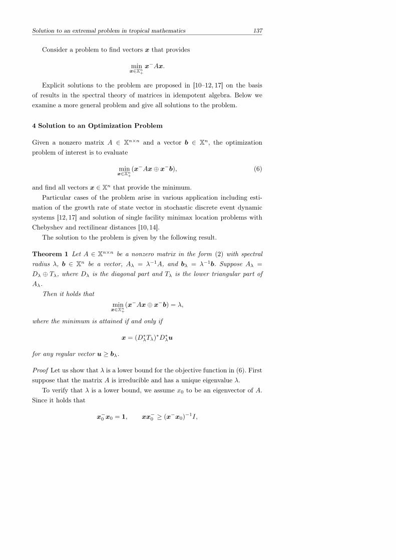
Solution to an extremal problem in tropical mathematics 137
Consider a problem to find vectors x that provides
minx∈Xn+
x−Ax.
Explicit solutions to the problem are proposed in [10–12, 17] on the basisof results in the spectral theory of matrices in idempotent algebra. Below weexamine a more general problem and give all solutions to the problem.
4 Solution to an Optimization Problem
Given a nonzero matrix A ∈ Xn×n and a vector b ∈ Xn, the optimizationproblem of interest is to evaluate
minx∈Xn+
(x−Ax⊕ x−b), (6)
and find all vectors x ∈ Xn that provide the minimum.Particular cases of the problem arise in various application including esti-
mation of the growth rate of state vector in stochastic discrete event dynamicsystems [12, 17] and solution of single facility minimax location problems withChebyshev and rectilinear distances [10,14].
The solution to the problem is given by the following result.
Theorem 1 Let A ∈ Xn×n be a nonzero matrix in the form (2) with spectralradius λ, b ∈ Xn be a vector, Aλ = λ−1A, and bλ = λ−1b. Suppose Aλ =
Dλ ⊕ Tλ, where Dλ is the diagonal part and Tλ is the lower triangular part ofAλ.
Then it holds that
minx∈Xn+
(x−Ax⊕ x−b) = λ,
where the minimum is attained if and only if
x = (D∗λTλ)∗D∗λu
for any regular vector u ≥ bλ.
Proof Let us show that λ is a lower bound for the objective function in (6). Firstsuppose that the matrix A is irreducible and has a unique eigenvalue λ.
To verify that λ is a lower bound, we assume x0 to be an eigenvector of A.Since it holds that
x−0 x0 = 1, xx−0 ≥ (x−x0)−1I,
138 N. Krivulin
for all x ∈ Xn+ we have
x−Ax⊕ x−b ≥ x−Axx−0 x0 ≥ x−Ax0(x−x0)
−1 = λx−x0(x−x0)
−1 = λ.
Now consider an arbitrary matrix A in the form (2). Take any vector x ∈ Xn+and split it into subvectors x1, . . . ,xs according to the row partition of A. Byapplying the previous result for irreducible matrices, we get
x−Ax⊕ x−b ≥ x−Ax ≥s⊕i=1
s⊕j=1
x−i Aijxj ≥s⊕i=1
x−i Aiixi ≥s⊕i=1
λi = λ.
Let us find all regular solutions of the equation
x−Ax⊕ x−b = λ.
Under the condition x−Ax⊕x−b ≥ λ for all x ∈ Xn+, the solutions coincidewith those of the inequality
x−Ax⊕ x−b ≤ λ.
It is not difficult to see that the last inequality is equivalent to the inequality
Aλx⊕ bλ ≤ x.
Indeed, multiplication of both sides of this inequality by λx− gives the firstinequality. On the other hand, by multiplying the first inequality by λ−1x andusing that xx− ≥ I, we have
Aλx⊕ bλ ≤ λ−1xx−Ax⊕ λ−1xx−b ≤ x,
and thus arrive at the second inequality.
By applying Lemma 1 to this inequality, we get the solution
x = (D∗λTλ)∗D∗λu,
where u is any regular vector such that u ≥ bλ.
References
1. F. L. Baccelli, G. Cohen, G. J. Olsder, J.-P. Quadrat, Synchronization and linearity: Analgebra for discrete event systems, Wiley, Chichester, 1993.
2. R. A. Cuninghame-Green, Minimax algebra and applications, Advances in Imaging andElectron Physics, Vol. 90 (1994), Academic Press, San Diego, pp. 1–121.
3. V. N. Kolokoltsov, V. P. Maslov, Idempotent analysis and its applications, Kluwer, Dor-drecht, 1997.
4. J. S. Golan, Semirings and affine equations over them: Theory and applications, Springer,New York, 2003.
5. B. Heidergott, G. J. Olsder, J. van der Woude, Max-Plus at work: Modeling and analysisof synchronized systems, Princeton Univ. Press, Princeton, 2005.
6. G. L. Litvinov, The Maslov dequantization, idempotent and tropical mathematics: Abrief introduction, Journal of Mathematical Sciences 140 (2007), no. 3, 426–444. E-printarXiv:math.GM/0507014.
7. P. Butkovic, Max-linear systems: Theory and algorithms, Springer, London, 2010.8. P. Butkovic, A. Aminu, Introduction to max-linear programming, IMA Journal of Man-
agement Mathematics 20 (2008), no. 3, 233пїЅ-249.9. S. Gaubert, R. D. Katz, S. Sergeev, Tropical linear programming and parametric mean
payoff games, to be published in Journal of Symbolic Computation, 2012. E-printarXiv:1101.3431.
10. N. K. Krivulin, An algebraic approach to multidimensional minimax location problemswith Chebyshev distance, WSEAS Transaction on Mathematics 10 (2011), no. 6, 191–200.
11. N. K. Krivulin, Eigenvalues and eigenvectors of matrices in idempotent algebra, VestnikSt. Petersburg University: Mathematics 39 (2006), no. 2, 72–83.
12. N. K. Krivulin, Methods of idempotent algebra in problems of complex systems modelingand analysis, St. Petersburg Univ. Press, St. Petersburg, 2009. (in Russian)
13. N. K. Krivulin, A new algebraic solution to multidimensional minimax location problemswith Chebyshev distance, to be published in WSEAS Transaction on Mathematics, 2012.
14. N. K. Krivulin, An extremal property of the eigenvalue for irreducible matrices in idempo-tent algebra and an algebraic solution to a Rawls location problem, Vestnik St. PetersburgUniversity: Mathematics 44 (2011), no. 4, 272–281.
15. K. Zimmermann, Disjunctive optimization, max-separable problems and extremal algebras,Theoretical Computer Science 293 (2003), no. 1, 45–54.
16. A. Tharwat, K. Zimmermann, One class of separable optimization problems: Solutionmethod, application, Optimization 59 (2008), no. 5, 619–625.
17. N. K. Krivulin, Evaluation of bounds on the mean rate of growth of the state vectorof a linear dynamical stochastic system in idempotent algebra, Vestnik St. PetersburgUniversity: Mathematics 38 (2005), no. 2, 42–51.
18. N. K. Krivulin, Solution of generalized linear vector equations in idempotent algebra,Vestnik St. Petersburg University: Mathematics 39 (2006), no. 1, 16–26.
Nikolai KrivulinS.-Petersburg State University, S.-Petersburg, RussiaE-mail: [email protected]
Tropical and Idempotent Mathematics. Moscow, Russia, August 26–31, 2012
Versions of the Engel theorem for semigroups
G. L. LitvinovG. B. Shpiz
1. Nilpotent and quasinilpotent semigroups
Let S be an abstract semigroup with a subsemigroup S0. We shall say thatS is an n-extension of its subsemigroup S0 if every product of n elements ofS is an element of S0; in this case we shall say that S is quasinilpotent if S0
is commutative. The semigroup S is called nilpotent if it is quasinilpotent forS0 consisting of a single zero element 0, so Sn = 0, see [5]. Of course, everycommutative semigroup is quasinilpotent.
2. Versions of the Engel theorem for semigroups in traditional math-ematics
Theorem 1 Let S be a nilpotent or quasinilpotent semigroup of finite dimen-sional complex matrices. Then there exists a common nonzero eigenvector forall elements of S.
Theorem 2 Let S be a nilpotent or quasinilpotent semigroup of finite dimen-sional matrices with nonnegative entries. Then there exists a common nonzerononnegative eigenvector for all elements of S.
This result is a generalization of the the well known Perron-Frobenius theo-rem.
Versions of the Engel theorem for semigroups 141
3. Nilpotent and quasinilpotent semigroups of operators inArchimedean tropical linear spaces
We use the terminology from [2, 3, 6] and discuss semigroups of operators inb-complete linear idempotent spaces over the tropical semifield Rmax, i.e. intropical linear b-complete spaces. Let V and W be spaces of this type. We shallsay that a linear operator A : V →W is continuous if A(supX) = supA(X) andA(infX) = inf A(X) for every bounded linearly ordered subset X in V (withrespect to the corresponding induced order). Note that every operator of thistype is b-linear.
A linear functional φ on V is called bounded, if the set x ∈ V |φ(x) 1 isbounded.
The space V is called Archimedean [6], if there exists a bounded continuouslinear functional f on V such that f(x) is nonzero for every nonzero x ∈ V .Examples of Archimedean spaces can be found in [3, 6].
Theorem 3 Let S be an arbitrary set of commuting continuous linear operatorson an Archimedean space V . Then there exists a common nonzero eigenvectorfor all elements of S.
Theorem 4 Let S be a nilpotent or quasinilpotent semigroup of continuous lin-ear operators on an Archimedean space. Then there exists a common nonzeroeigenvector for all elements of S.
The following result is a trivial corollary of this theorem.
Theorem 5 Let S be a nilpotent or quasinilpotent semigroup of finite dimen-sional matrices with tropical entries. Then there exists a common nonzero eigen-vector for all elements of S.
Note that our Theorems 2 and 5 extend a result of Katz, Schneider andSergeev [1] on existence of a joint eigenvector of several commuting matrices. Adifferent theorem on existence of a joint eigenvector for all matrices in a "nice"semigroup consisting of strongly regular matrices over the tropical semifield wasrecently obtained by Merlet [4].
The authors thank S.N. Sergeev for his comments and references.
References
1. Katz R.D., Schneider H., Sergeev S. On commuting matrices in max algebra and in non-negative matrix algebra // Linear Algebra and its Applications, vol. 436, issue 2, 2012,276-292.
2. Litvinov G.L., Maslov V.P., Shpiz G.B. Idempotent Functional Analysis. An algebraicapproach //Mathematical Notes, vol. 69, No.5, 2001, p. 696–729. E-print math.FA/0009128(http://arXiv.org).
3. Litvinov G.L., Maslov V.P., Shpiz G.B. Idempotent (asymptotic) mathematics and therepresentation theory. - In: V.A. Malyshev and A.M. Vershik (eds.), Asymptotic Combina-torics with Applications to Mathematical Physics. Kluwer Academic Publishers, Dordrechtet al, 2002, p. 267-278. E-print math.RT/0206025 (http://arXiv.org).
4. Merlet G. Semigroup of matrices acting on the max-plus projective space, Linear Algebraand its Applications, vol. 433, issue 8, 2010, 1923-1935.
5. Nilpotent semi-group. – In: Encyclopedia of Mathematics. E-printhttp://www.encyclopediaofmath.org
6. Shpiz G.B. A theorem on eigenvectors in idempotent spaces // Doklady Mathematics, vol.62, No.2, 2000, p. 169–171.
This work is supported by the grant RFBR 12-01-00886-a and the jointRFBR-CNRS grant 11-01—93106-a.
G. L. LitvinovThe A. A. Kharkevich Institute for Information Transmission Problems RASand the Poncelet Laboratory, Moscow, Russia.E-mail: [email protected]
G. B. ShpizMoscow State University, Moscow, Russia.E-mail: [email protected]
Tropical and Idempotent Mathematics. Moscow, Russia, August 26–31, 2012
Tropical computations in Mathpar
Gennadi Malaschonok
1 Introduction
Objects studied in physics, chemistry, biology require more precise and efficientmeans to describe and create adequate mathematical models. Instead of simplenumerical models popular in the past, we now have analytical models that requireadvanced analytical tools for their construction.
Computer algebra systems like MAPLE, Mathematica, CoCoA, Reduce, etc.,designed for single-core machines do not allow to create compound analyticalmodels. New software tools designed for SPMD Cluster Computing with thou-sands of nuclei are required today.
The history of numerical linear algebra packages (ScaLAPAC, LAPAC andothers) shows that multi-processor systems require the creation of new soft-ware systems for which the data structures and algorithms have been initiallyfocused on parallel computing systems. So we need a fundamentally new paral-lel programming systems for numerically-analytical calculations, in which datastructures and algorithms will be designed for supercomputers.
There are several fundamental symbolic matrix algorithms developed duringthe last 20 years, with the same computational complexity as in the algorithmsof matrix multiplication. These algorithms are basic for solving linear algebraproblems in the commutative domains and in the domains of principal ideals.Most of these algorithms are implemented as parallel MPI-programs.
Mathpar is a computer algebra system aimed at performing computations inarbitrary algebras with high efficiency.
144 G. Malaschonok
The Mathpar language is called ATeX. This is an active version of the TeXlanguage, allowing to perform operations and to write procedures and functionslike in TeX. Mathpar is a web service at http://mathpar.com. A tutorial ofMathpar and many help pages of this on-line mathematical service can be foundon this website. In addition to traditional algebra you can perform calculationsin idempotent algebras. This is the subject of the present report.
2 Environment for mathematical objects
The definition of any mathematical object, a number or a function, a matrix ora symbol, involves the definition of some environment, that is, the space whichcontains this object. To select the environment you have to set the algebraicstructure. This algebraic structure is defined by numeric sets, algebraic opera-tions in these sets and variable names.
First of all, any user has to set an environment in Mathpar. By default,the space of six integer variables Z[x, y, z]Z[u, v, w] is defined. This is a ringof polynomials with coefficients in the ring of integer numbers. The variablesare divided into two groups of three variables: variable x is the “youngest”, andvariable w is the “eldest”. The variables are arranged from left to right.
User can change the environment, setting a new algebraic structure. For ex-ample the space R64[x, y, z] may be suitable to solve many problems of compu-tational mathematics. The installation command should be as follows: “SPACE= R64 [x, y, z]; ”.
Moving a mathematical object from the previous environment to the currentenvironment is performed explicitly, using the toNewRing() function. In somecases, such a transformation to the current environment is automatic.
All other names not listed as variables can be chosen by the user arbitrarily,for any mathematical object.
For example
a = x+ 1, f = \sin(x+ y)− a.
There is a rule to distinguish between commutative and noncommutative alge-bra. If the object name begins with a capital letter, then the object is an elementof a noncommutative algebra. If the object name begins with a lowercase letter,then the object is an element of a commutative algebra.
Tropical computations in Mathpar 145
3 Numerical sets with standard operations
Current version of the system supports the following numerical sets with stan-dard operations.
Z — the set of integers Z,Zp — a finite field Z/pZ where p is a prime number,Zp32 — a finite field Z/pZ where p is less 231,Z64 — the ring of integer numbers z such that −263 6 z < 263,Q — the set of rational numbers,R — the set of floating point numbers to store approximate real numbers
with arbitrary mantissa,R64 — standard floating-point 64-bit numbers (52 digits for mantissa, 11 bits
for the order and 1 bit for the sign),R128 — standard floating-point 64-bit numbers, equipped with optional 64-
bit for the order,C — complexification of R,C64 — complexification of R64,C128 — complexification of R128,CZ — complexification of of Z,CZp — complexification of Zp,CZp32 — complexification of Zp32,CZ64 — complexification of Z64,CQ — complexification of Q.Examples of simple commutative polynomial rings:
SPACE = Z [x, y, z]; SPACE = R64 [u, v]; SPACE = C [x].
4 Several numerical sets
The ring Z[x, y, z]Z[u, v, w], which has two subsets of variables, is the polynomialring with variables u, v, w with coefficients in the polynomial ring Z[x, y, z].
For example, the characteristic polynomial of a matrix over the ring Z[x, y, z]can be obtained as a polynomial of variable u, whose coefficients are polynomialsin the ring Z[x, y, z].
You can set algebraic space which defines several numerical sets. For example,the space C[z]R[x, y]Z[n, m] allows to have five names of variables, which belongto the sets C, R and Z, respectively. The first set is the main one.
C[z]R[x, y]Z[n,m] can be viewed as a polynomial ring of five variables overC, with additional properties. If the polynomial does not contain variables z, x,
146 G. Malaschonok
y, then it is a polynomial with coefficients in the set Z. If the polynomial doesnot contain z, then it is a polynomial with coefficients in R. Examples:SPACE=Z[x, y]Z[u]; SPACE=R64[u, v]Z[a, b]; SPACE=C[x]R[y, z];
5 Group algebras
Group algebra is defined as KG, where K is a commutative ring of scalars andG — is a group of noncommutative operators with finite number of generators.Names of these generators should begin with capital letters.
For example, the following group algebras can be defined:SPACE = Z[x, y]G[U, V ]; (generators U, V),SPACE = R64[u, v]G[A,B]; (generators A, B),SPACE = C[]G[X,Y, Z, T ]; (generators X, Y, Z, T).Each element of such algebra can be considered as a sum of terms with
functional coefficients.R64[t, y]G[X, Y, Z] is the free group algebra over a function field of two
variables t, y over the field R64 with three non-commuting generators X, Y, Z.For example, A = (t2 + 1)X + sin(t)Y + 3X2y3 + (t2 + 1)XY 3X2Y −2X2 is anelement of such algebra.
6 Constants
It is possible to set or replace the following constants.ACCURACY — the amount of exact decimal positions in the fractional part
of real numbers of type R resulting from multiplication or division operation.FLOATPOS —the amount of decimal positions of real number of type R or
R64, which you can see in the printed form.ZERO_R — the machine zero for R and C numbers.ZERO_R64 — the machine zero for R64, R128, C64 and C128 numbers.MOD32 — the module for a finite field of type Zp32, its value is not greater
than 231.MOD — the module for a finite field of type Zp.To set the machine zero to 1/109 (i.e., 1E − 9), you can use the commands
ZERO_R = 9 or ZERO_R64 = 9.
Example.SPACE=Zp32[x, y]; MOD32=7;
f1=37x+42y+55; f2=2f1;
\print(f1, f2 );
Tropical computations in Mathpar 147
The results: f1 = 2x− 1; f2 = 4x+ 5.
7 Idempotent algebra and tropical mathematics
Idempotent/tropical algebras can be used as well. In this case the signs of "ad-dition" and "multiplication" for the infix operations can be used for operationsin tropical algebra: min, max, addition, multiplication.
Each numerical set R, R64 or Z has two additional elements∞ and −∞, andtwo elements that play the role of zero and unit. We denote these sets R, R64, Z,respectively. The name of idempotent algebra consists of three components: (1)the numerical set, (2) the operation corresponding to plus and (3) the operationcorresponding to times.
For example, algebras R64MaxPlus, R64MinPlus, R64MaxMin,R64MinMax, R64MaxMult, R64MinMult are defined over the numeri-cal set R64.
RMaxPlus, RMinPlus, RMaxMin, R64MinMax, RMaxMult, RMinMult aredefined over the numerical set R.
ZMaxPlus, ZMinPlus, ZMaxMin, ZMinMax, ZMaxMult, ZMinMult are de-fined over the numerical set Z.
Let us give an example of tropical arithmetics in ZMaxPlus.
Example.
SPACE=ZMaxPlus[x, y];
a=2; b=9+x; c=a+b; d=a*b+y; \print(c, d)
Results: c = x+ 9; d = y + 2 ∗ x+ 11.For each algebra we defined elements 0 and 1, −∞ and ∞. For each element
a we defined the operation of closure (Kleene star): a× = 1 + a + a2 + a3 + ....This operation is an analogue of the classical (1− a)−1.
8 The calculations on a supercomputer
In order to solve computational problems that require large computation time orlarge amounts of memory, the system has special functions that provide the userwith resources of supercomputer. These functions allow you to perform calcula-tions not on a single processor and on a dedicated set of cores of supercomputer.The number of cores is ordered by the user.
You have the following functions ( parfunctions) that can be performed onsupercomputer:
1) gbasisPar — computation of Grobner basis;2) adjointPar — computation of adjoint matrix;3) adjointDetPar — computation of adjoint matrix and determinant of a matrix;4) echelonFormPar — computation of matrix echelon form;5) inversePar — computation of inverse matrix;6) detPar — computation of determinant of a matrix;7) kernelPar — computation of kernel of a linear operator;8) charPolPar — computation of characteristic polynomial;9) multiplyPar — calculation of matrix product;10) multiplyPar — computation of product of polynomials.
Before applying any of these functions, the user has to specify some param-eters that define the parallel environment:
TOTALPROCNUMBER — total number of processors (cores) providedfor the computations,
NODEPROCNUMBER — number of cores on a single node,CLUSTERTIME — maximum time (in minutes) which you allow for a
program to execute (after which it is forced to end).To set the number of cores on a single node the user has to know which
cluster is used and how many cores are available on the node. By default, theTOTALPROCNUMBER and NODEPROCNUMBER are set so that allavailable cores are used by the node, and CLUSTERTIME = 1.
The user can change the number of cores on one node. This is an importantfeature, since the memory on a node is used by all cores on this node. Conse-quently, the user can regulate the size of RAM that is available at one core. Fornow, only users of the cluster of Tambov State University can perform parallelcomputing.
References
1. G. I.Malaschonok, Project of Parallel Computer Algebra, Tambov University Reports.Series: Natural and Technical Sciences. 15. Issue 6. (2010), 1724–1729.
2. G. I.Malaschonok, Computer mathematics for computational network Tambov UniversityReports. Series: Natural and Technical Sciences. 15 Issue. 1. (2010), 322–327.
3. G. I.Malaschonok, On the project of parallel computer algebra, Tambov University Re-ports. Series: Natural and Technical Sciences. 14 Issue. 4. (2009), 744–748.
Gennadi MalaschonokTambov State UniversityE-mail: [email protected]
Tropical and Idempotent Mathematics. Moscow, Russia, August 26–31, 2012
Powers of matrices with an idempotent operationand an application to dynamics of spatial agglom-erations
Vladimir Matveenko
Abstract The paper develops an approach to analyze dynamics of economicnetwork structures with a considerable role of externalities, such as spatialagglomerations. The approach is based on a use of powers of matrices with anidempotent operation.
1 An idempotent algebraic model of economic development withpositive externalities
The scheme of dynamic programming was studied by many authors beginningfrom Bellman [1] and probably most explicitly by Romanovsky [10] who showedthat a sufficiently long T -step optimal path in its initial part is characterized bya so called (first) system of potentials which is a version of the Bellman’s valuefunction, and by use of this function the first part of the optimal path (up to itsentrance into the turnpike) can be constructed stepwise. However these authorshave missed some other natural and principally important conclusions. Similarlyto the initial part, the final part of the path can be constructed "backward" (inthe inverse time) stepwise by use of a function which can be referred to as thesecond system of potentials or the second value function. The latter correspondsthe left eigenvector of the matrix of utilities in an algebra with an idempotent
150 V. Matveenko
operation, while the first value function corresponds the right eigenvector. EachT -step optimal path under sufficiently large horizon T has a three-part structurewhich corresponds to the structure of the T -th power (with the idempotentoperation) of the matrix of utilities (see [9]).
One of dynamic objects which can be modeled by use of the powers of a ma-trix with idempotent operation is an economic system with mutual externalities.
Externality is "any indirect effect that either a production or a consumptionactivity has on a utility function, a consumption set, or a production set. By "in-direct" we mean both that the effect is created by an economic agent other thanthe one who is affected and that the effect is not transmitted through prices"( [5], p. 6). The role of externalities in spatial structures, such as countries, re-gions and cities, has been stressed by many authors following Marshall [7] whoconsidered industry-specific district externalities as ensuring specialization andeconomies of scale. Jacobs [3] argued that knowledge can spill over between dif-ferent complementary industries in the same location. Such sort of externalitiesis often referred as ’Jacobian’. Lucas [6] called them ’externalities of creative pro-fessions’. These externalities are not limited only by knowledge but can relateto any forms of mutual influence and dependence.
In [8] individual possibilities of the agents to develop can be limited by aninsufficiency of the sizes of externalities created by other agents.
Let i = 1, · · · , n be economic agents (firms, authorities, groups of labor ofdifferent types, etc.). Each agent i in period t is characterized by a single positivenumber xti referred as her value. It can be, for example, profit, income, welfare,present value, knowledge, etc. Development of the i-th agent is being describedas changes in her value in discrete time. We make two assumptions:
1. Development of the i-th agent is limited by her own potential possibilitiesdescribed by a fixed growth factor aii > 0:
xt+1i ≤ aiixti, t = 0, 1, · · · ; i = 1, · · · , n;
2. Development of the i-th agent is limited by limitations on positive external-ities created by some other agents:
xt+1i ≤ aijxtj , j = 1, · · · , n, j 6= i, t = 0, 1, · · · ; i = 1, · · · , n;
where aij are coefficients describing limitations for the i-th agent’s developmentcaused by bounds of the positive externalities created by the j-th agent. Hereaij = +∞ if agent j creates no externality used by agent i or if the externalitycreated by j never becomes binding for i. An externality is called nonbiding for
Powers of matrices 151
an agent if it currently does not limit her development, i.e. the development islimited either by the agent’s own growth factor or by another externality. Anexternality is binding if the development is currently limited by the externality.
If each agent maximizes her value stepwise under the present constraintsthis results in the following equations characterizing the equilibrium path giveninitial values x0
1, · · · , x0n :
xt+1i = min
j=1,··· ,naijx
tj , t = 0, 1, · · · ; i = 1, · · · , n
which in terms of idempotent mathematics can be easily written as
xt+1 = A⊗ xt, t = 0, 1, · · ·
where A = (aij) is an n × n-matrix, xt, xt+1 are positive n-vectors, and theproductA⊗xt is a product of a matrix and a vector with an idempotent operation⊕ = min and usual multiplication.
The behavior of the system xt = At⊗x0, t = 1, 2, · · · , where At = A⊗· · ·⊗A,is totally defined by properties of the matrix A. The system can demonstratedifferent patterns such as convergence to an eigenvector with stable growth fac-tor, stable decline, convergence to a limit cycle, etc. An important result is thatoften a small change in an element of the matrix A can lead to a radical changeof a pattern of behavior of the system (so called butterfly effect or catastrophicbifurcation).
It is important to notice that an externality can be nonbinding until an agenti is "small" but when the agent "grows up" she can face the limitation of aninsufficient development of another agent or a group of agents.
An agent facing a binding externality could be interested in making paymentsimproving her development. These payments can have numerous forms such asa redistribution of incomes through a mechanism of taxes and transfers, directsupply of products and resources (e.g., in form of barter or credit), supply ofprivileges, providing information, or, simply, bribes. However, as is seen fromthe model, a choice of a suitable direction of payment is a serious problem forthe agent, which can have political consequences.
A model variable changeable coefficients can be considered. In a simple case itcan be assumed that agent i is able to diminish her own development coefficient,aii, and, instead, to increase a development coefficient aij of any other agent ora coefficient of externality constraint akl for any pair of agents, k,l.

152 V. Matveenko
More realistic is a situation of tranferable values where agents are able toexchange not their development coefficients but values. For a model with matrix
A =
2 1 +∞+∞ 2 1
+∞ +∞ 0.6
under the absence of redistribution the path leads to a proportional decline witha growth rate 0.6. Let the agents be able to partially exchange their values, andlet the direction and the value of transfers be defined by the 1st agent (e.g. shehas a majority in a parliament).
The 1st agent feels an externality from the side of the 2nd one, that is whyshe is interested in payments to the 2nd agent. In such case the 1st agent caresabout maximization of her next current value; for her, as can be checked, it willbe optimal to support the value of the 2nd agent on a level twice more than herown level. Such strategy leads to a temporary increase in the value of the 1stagent and then to a decline slower than under the absence of payments . Thevalues of the 3rd agent are not touched by this policy at all.
However, there exists a possibility of a long-run growth of the whole systemif the transfers are directed from the 1st agent not to the 2nd but to the 3rdone.
Notice that in this example an "optimal" (from the long-run point of view)governmental redistribution policy leads to a long-run growth of all agents, how-ever, it does not give a short-run gain to the 1st agent, which defines a choiceof a policy. If a subjective discounting coefficient of the 1st agent is not highenough, she will prefer a short-run gain, which will lead to a long-run decline.
The case, when the 1st agent executes a transfer to the 2nd agent whoseinsufficient externality is filled, can be also interpreted as a bribe, and a case,when a transfer is received by the 3rd agent with whom the 1st agent is notlinked directly, as a result of an action of a fiscal system. Thus the model showsthat the corruption provides an agent an evident gain in a short run but it doesnot prevent a decline in a long run. The governmental redistribution policy, inits turn, leads to a growth of all agents but provides no short-run gain to the1st agent. Under a small subjective discount factor, the 1st agent will prefer ashort-run gain which can be achieved through tax-avoiding and bribes.
In a general case of n agents, the model can be used to provide a choice ofagents to be taxed and to define optimal values of taxes and transfers.
Powers of matrices 153
2 A model of spatial development
The approach can be applied to explaining such processes in spatial economicsystems as migration of production factors, agglomeration and de-agglomeration(dispersion). Johansson and Quigley [4] in their discussion of agglomerationsand networks mark that in the agglomeration economies externalities usuallyhave a character of public good, while in the periphery market network relationsprevail with a distribution of private institutional capital among the participants.("When co-location is infeasible, networks may substitute for agglomeration").However, these authors only mention a unity of the mechanisms of agglomerationand networking and do not explain the reasons of the difference in behavior ofeconomic agents in the core and in the periphery. We try to answer this questionhere.
The specific character of the spatial economies lies in much in the presenceof two ample sets of economic agents: (i) stationary agents condensed and ac-complishing their activities permanently in definite points or areas in space, and(ii) free agents who are able to move their activities in the space more easily.Economic processes of the locational movement of productive factors and con-sumers, such as migration, offshoring, agglomeration and de-agglomeration canbe represented as moves of the free agents generated by dynamics of economicstructures connected first of all with the effectiveness of the stationary agents.From dynamics perspective these structures are related first of all with numerousmutual externalities created by agents in their locations. The concentrations ofagents of different types is the most important characteristic of any geographiclocation.
As a simplest example of such dynamic model let us consider the case oftwo stationary agents: 1 in a core, 2 in a periphery and one free agent: 3. Theindividual potential growth factor of a stationary agent in the core is higherthan in the periphery: a11 > a22. Let a11 = 1.2, a22 = 1.5, a33 = 1.5, a31 =
0.4, a32 = 2. Other four elements of the matrix A are equal to aij = +∞ . Thedynamics of the free agent is described by the equation:
xt+13 = mina33x
t3,maxa31x
t1, a32x
t2.
Let the free agent be initially in the core, and let the initial state of themodel be (x0
1 = 2, x02 = 0.7, x0
3 = 0.5) . The free agent faces initially no externallimitation, but on step 1 she faces a binding external limitation in the coreand moves to the periphery. On step 2 she acts in the periphery and does notface binding external limitations there. Further on steps 3-6 she faces a binding
154 V. Matveenko
limitation of an insufficient externality but still prefers to stay in the periphery.However, on step 7 the free agent chooses to return to the core.
The next stage of the research is introducing transferable values: now theagents are allowed to transfer a part of their values to other agents. These trans-fers, in particular, can be in form of an aid, an investment, a tax, a bribe, etc. Incase of transferable values, growth rates of all agents and locations of free agentsare endogenous variables.
To continue the example, if the free agent is interested in maximization ofher own growth (but not in the maximal current value as previously) and if shecan share her value with a stationary agent, she stays forever in the peripheryand the periphery starts developing faster than the core.
It can be shown that the growth factor of the system, consisting of a station-ary agent i = 1 or i = 22 (the cases when the stationary agent is either in thecore or in the periphery) and a free agent 3, is equal to
ai3 =a33(aii + a3i)
a33 + a3i.
It follows that the condition that the periphery is more preferable for thefree agent than the core is
a11 + a31
(1− a22
a33
)< a22 + a32
(1− a11
a33
).
The resulting index of the i-th region,
aii + a3i
(1− ajj
a33
), j 6= i,
includes terms related to the region’s "stationary" growth factor, aii , the exter-nality limitation in the region, a3i , as well as (with opposite sign) the relativegrowth factor in the alternative location, ajja33 .
Interesting are situations when behavior of free agents such as groups ofqualified labor depend on behavior of free firms. First free firms move to theperiphery and after some time the free qualified labor also tends to move to theperiphery. An important question is identifying conditions under which all ofthem return to the core and those conditions under which they stay forever inthe periphery. Both forward linkages in terms of Krugman [2] (the incentive ofworkers to be close to the producers of consumer goods) and backward linkages(the incentive of producers to concentrate where the market is larger) can beeasily taken into account in the model.
Trade between cities, regions or countries also can be included into thepresent model. To do this, a part of the coefficients aij can be interpreted as

limitations related to potential trade flows between the agents, and if these flowsare actualized it means presence of trade between the areas.
The model provides also an insight to policy analysis. For example, tradeliberalization and FDI can lead to an appearance of new external links, inparticular, in the periphery.
References
[1] R. Bellman Dynamic programming. Princeton: Princeton University Press, 1957.[2] M. Fujita, P. Krugman. The new economic geography: past, present, and the future. PapersReg. Sci. bf83 (2004), 139–164.
[3] J. Jacobs The economy of cities. New York: Random House, 1969.[4] B. Johansson and J.M. Quigley Agglomeration and networks in spatial economies. PapersReg. Sci. 83 (2004), 165–176.
[5] J.-J. Laffont. Fundamentals of public economics. Cambridge, MA: MIT Press, 1988.[6] R.E. Lucas. On the mechanics of economic development. Journal of Monetary Economics
22 (1988), 3–42.[7] A. Marshall Principles of economics. London: Macmillan, 1890.[8] V. Matveenko Development with positive externalities: The case of the Russian economy.Journal of Policy Modeling 17 (1995), 207-221.
[9] V. Matveenko Optimal paths in oriented graphs and eigenvectors in max-⊗ systems. Dis-crete Mathematics and Applications 19 (2009), 389-409.
[10] J.V. Romanovsky Optimization of stationary policy of discrete deterministic process.Kibernetika 2 (1967), 71-83 (In Russian).
Vladimir MatveenkoNational Research University Higher School of EconomicsE-mail: [email protected]
Tropical and Idempotent Mathematics. Moscow, Russia, August 26–31, 2012
Games of network disruption and idempotent al-gorithm complexity
William M. McEneaneyAntoine Desir
Abstract We consider a game on the space of network disruptions. An appli-cation in command and control is used as a guide for the development of themodel. The outcome of any set of physical actions depends on the informationavailable to the controller. We suppose that information flows along a networkof humans and machines. The opposing player may act to intermittently blockinformation flow along the network. This may be combined with physical actionssuch that our controller might be making decisions based on information thatis not as current as would be possible without the induced delays. We findthat the model of information delay dynamics is best captured as a controlledmin-plus linear system. We also find that the minimax value function may berepresented as a min-plus convex functional over the space of delay vectors. Thisis a max-min linear space. Backward dynamic programming propagation of thevalue function leads to (max-min) sum and product compositions. This yields aparticularly nice solution algorithm. Computational and solution-representationcomplexity are examined.
1 Introduction
We consider a game on the space of network disruptions. An application in com-mand and control is used as a guide for the development of the model. However,
Games of network disruption and idempotent algorithm complexity 157
it should be clear that the problem class addressed by the theory is much larger.There is a physical domain via which the ultimate rewards are obtained. Theoutcome of any set of physical actions depends on the information available tothe controller. We suppose that information flows along a network of humansand machines, where information processing may occur may occur at some ofthe nodes. The opposing player may act to intermittently block information flowalong the network. This may be combined with physical actions such that ourcontroller might be making decisions based on information that is not as currentas would be possible without the disruption.
We will find that the model of information delay is best captured as a min-plus linear system. Specifically, the delay of information from node g at node γis the minimum over the delays along available information-routes from node gto node γ. The opposing control may act to increase delays while our controllermay seek to reduce such delays, leading to a game with controlled min-plus lineardynamics.
We will find that the value function may take the form of a min-plus con-vex functional over the space of delay vectors. Note that in this componentof the analysis, we work in min-plus vector spaces. Recall that the space ofstandard-sense convex functions is a max-plus linear space (c.f., [12]), wherefinite-complexity convex functions are those given as pointwise maxima of a fi-nite set of standard-sense affine functions. That is, they may be represented asmax-plus linear combinations of standard-sense linear functions. In the workhere, the standard-sense algebra is replaced by the min-plus algebra and themax-plus algebra is replaced by the max-min algebra. Consequently, min-plusconvex functions are represented as max-min linear combinations of min-pluslinear functions.
We will want to consider larger scale networks. Thus, the complexity of thesolution representation is a critical question. We are led to questions of thecomplexity of max-min sums and products of finite-complexity min-plus func-tions. We find that this complexity grows more slowly that one would intuitivelyexpect. We also consider max-min linear projections as a means of complexity-growth attenuation.
2 Motivational Application
We will refer to the figure given below. Suppose there exists a network consist-ing of sensing nodes, action nodes, communication nodes and processing/decisionnodes. An example is given in the figure. The network may be considered to be
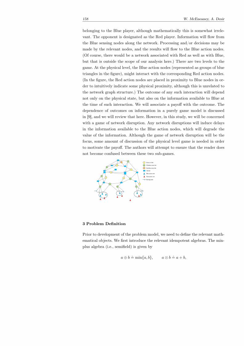
158 W. McEneaney, A. Desir
belonging to the Blue player, although mathematically this is somewhat irrele-vant. The opponent is designated as the Red player. Information will flow fromthe Blue sensing nodes along the network. Processing and/or decisions may bemade by the relevant nodes, and the results will flow to the Blue action nodes.(Of course, there would be a network associated with Red as well as with Blue,but that is outside the scope of our analysis here.) There are two levels to thegame. At the physical level, the Blue action nodes (represented as groups of bluetriangles in the figure), might interact with the corresponding Red action nodes.(In the figure, the Red action nodes are placed in proximity to Blue nodes in or-der to intuitively indicate some physical proximity, although this is unrelated tothe network graph structure.) The outcome of any such interaction will dependnot only on the physical state, but also on the information available to Blue atthe time of such interaction. We will associate a payoff with the outcome. Thedependence of outcomes on information in a purely game model is discussedin [9], and we will review that here. However, in this study, we will be concernedwith a game of network disruption. Any network disruptions will induce delaysin the information available to the Blue action nodes, which will degrade thevalue of the information. Although the game of network disruption will be thefocus, some amount of discussion of the physical level game is needed in orderto motivate the payoff. The authors will attempt to ensure that the reader doesnot become confused between these two sub-games.
Server in link
Wireless voice link
Hardline voice link
Blue action unit
Red action unit
Sensing asset
Human
3 Problem Definition
Prior to development of the problem model, we need to define the relevant math-ematical objects. We first introduce the relevant idempotent algebras. The min-plus algebra (i.e., semifield) is given by
a⊕ b .= mina, b, a⊗ b .= a+ b,
Games of network disruption and idempotent algorithm complexity 159
operating on IR+ .= IR ∪ +∞. The max-plus algebra (i.e., semifield) is given
by
a⊕∨b .= maxa, b, a⊗∨b .= a+ b,
operating on IR−.= IR ∪ −∞. In the max-min algebra (i.e., semiring), the
operations are defined as
a ∨ b .= maxa, b, a ∧ b .= mina, b,
operating on IR .= IR ∪ −∞ ∪ +∞, where we note that −∞ ∨ b = b for all
b ∈ IR and −∞∧ b = −∞ for all b ∈ IR (c.f., [6]).
3.1 Payoff origin
We briefly describe the physical level game which will yield the payoff for thenetwork disruption game that is our main focus. This will be a zero-sum game.Consider time tk with k ∈]0,K[
.= 0, 1, 2 . . .K, where we note that throughout
we will use the notation ]a, b[ to denote a, a+ 1, a+ 2 . . . b for integers a ≤ b.Suppose that at this time, there is an interaction between the Blue and Red ac-tion nodes. The possible actions for Blue are denoted by v ∈ V =]1, V [. The trueRed action node configuration is x ∈ X =]1, X[. Given true asset configuration,x, Blue would obtain an action payoff c(x, v). Let C(v) be the vector of lengthX with components c(x, v).
It is natural to use the max-plus probability structure (c.f., [1, 4, 9, 14] andthe references therein) for deterministic games. (Note that, as with the networks,we model only the effect of Blue partial information.) Suppose Blue’s knowledgeof the true configuration is described by max-plus probability distribution, q ∈S⊕∨X , where
S⊕∨X .
=q ∈ [−∞, 0]X
∣∣∣⊕x∈X
∨qx = 0,
where [−∞, 0] denotes (−∞, 0] ∪ −∞ and the X superscript indicates outerproduct X times. (Also, the
⊕∨ symbol indicates max-plus summation.) It isuseful to recall that [−∞, 0] is analogous to [0, 1] in the standard algebra, where0 takes the place of 1 (the multiplicative identity), and −∞ takes the place of0 (the additive identity). We may interpret each component, qx, as the additiveinverse of the (relative) cost to Red to cause Blue to believe that the configurationis x. This will be become more clear below. The expected payoff for action v ∈ Vgiven max-plus distribution q at time tK , is as follows. Letting max-plus random
160 W. McEneaney, A. Desir
variable ξ be distributed according to q, and E⊕∨
q denote max-plus expectationaccording to this q, the expected payoff is
J(q, v) = E⊕∨
q [c(v, ξ)] =⊕x∈X
∨c(v, x)⊗∨qx = C(v)∨ q,
where ∨ denotes the max-plus dot product. Given that Blue wants to minimize(make more negative) the physical level payoff, the value of information q is
φ(q).= min
v∈VJ(q, v) =
∧v∈V
[C(v)∨ q]. (1)
We see that if information is represented by a max-plus probability distributionover a finite set (and one has a finite set of controls), then the value of informationtakes the form of a min-max sum of max-plus linear functionals over a max-plus probability simplex. We also emphasize again that the above game merelyprovides the payoff for the network disruption game to follow.
3.2 Network game dynamics
It may again be helpful to refer to our main figure (see above). We supposethat the Blue network will be defined as a graph, (G, E), where G denotes theset of nodes, and E denotes the set of edges. The set of nodes will be decom-posed as G = Gs ∪ Ga ∪ Gc ∪ Gd where Gs denotes the set of sensing nodes (airvehicle icons in the example figure), Ga denotes the set of action nodes (bluetriangular icons in the example figure), Gc denotes the set of communicationnodes (colored disc icons in the example figure) and Gd denotes the set of deci-sion/analysis nodes (blue rectangular icons in the example figure). Let G =]1, n[,and E = (g1
i , g2i ) | g1
i , g2i ∈ G ∀i ∈]1, ne[, where the elements of E are unordered
pairs. Let Gs = #Gs, Ga = #Ga, Gc = #Gc and Gd = #Gd. We supposethat for each action node, say α ∈ Ga, there exists a set of relevant sensingnodes, Gs(α) ⊆ Gs such that information from these sensing elements affectsthe min-plus probability distribution describing information relevant to actionnode α. Further, given α ∈ Ga and σ ∈ Gs(α), there exists an ordered set ofdecision/analysis nodes that information from σ must pass through prior to useby α. Let this path be denoted as
Iσ,α = (σ, g2, g3 . . . gn(σ,α)−1, α)
Games of network disruption and idempotent algorithm complexity 161
with gk ∈ Gd for all k ∈]2, n(σ, α)−1[. We also let Pσ,αN denote the set of orderedsequences of maximum length N given by
Pσ,αNγini=1
∣∣∣ n ∈]1, N [, (γi, γi+1) ∈ E ∀i ∈]1, n− 1[,
and s.t. ∃ subsequence γijn(σ,α)j=1 s.t. i1 = 1,
in(σ,α) = n, γij = gj ∈ Iσ,α ∀j ∈]1, n(σ, α)[.
Note that the elements of Pσ,αN are feasible paths through the graph passingthrough the required nodes of Iσ,α in the required order.
We now begin the discussion of the network disruption game. We use a fixedtime-step model where, without loss of generality, tk+1− tk = 1 for all k. Let thedelay in transfer of information along edge (γ, g) ∈ E be denoted by δeγ,g ∈ [0,∞),and the processing delay at node γ ∈ G be δpγ ∈ [0,∞). We let the delay at time tkin arrival of information originating from node σ ∈ Gs at node g ∈ G be denotedby dσg,k. We also let the vector of length n of such delays be dσk . The delays ininformation arrival originating at all nodes in Gs will be Dk = dσk |σ ∈ Gs.Notationally, it will be helpful to arrange Dk as a vector of length nGs. Ofcourse, there may be multiple routes from node σ to node g. For g ∈ G, letNg
.= γ ∈ G | (γ, g) ∈ E. It is easy to see that the dynamics of dσg,k are given
bydσg,k+1 =
∧γ∈Ng
δγ,g + dσg,k =⊕γ∈Ng
δγ,g ⊗ dσg,k, (2)
where δγ,g = δeγ,g + δpγ and the⊕
symbol denotes min-plus summation. Let Tbe the n× n matrix with elements
Tg,γ =
δγ,g if γ ∈ Ng,
+∞ otherwise.
Then,dσg,k+1 =
⊕γ∈G
Tg,γ ⊗ dσγ,k ∀σ ∈ Gs, g ∈ G,
and arranging this in vector form,
dσk+1 = T ⊗ dσk ∀σ ∈ Gs, (3)
where here ⊗ indicates min-plus matrix-vector multiplication. Also, letting Tbe the block-diagonal nGs × nGs matrix consisting of T blocks, with +∞ (themin-plus zero) elsewhere, we may write
Dk+1 = T ⊗Dk. (4)
162 W. McEneaney, A. Desir
Now suppose that Red may act to increase delays, and Blue may act tocounter this. For example, in the case of radio transmissions, short delays maybe induced by jamming, and with inclusion of intervening routers, delays mayalso be induced by other means. Finally, we arrive at
dσk+1 = T (ubk, urk)⊗ dσk ∀σ ∈ Gs, (5)
or, equivalently,Dk+1 = T (ubk, u
rk)⊗Dk, (6)
where the Blue and Red controls at time tk are ubk ∈ Ub and urk ∈ Ur, respectively,and where we assume U b = #Ub < ∞ and Ur = #Ur < ∞. Note that (5),or equivalently (6), will define the dynamics in the network disruption game.Importantly, we have a system with controlled (min-plus) linear dynamics.
3.3 Network game payoff and value
We now begin definition of the payoff for this game. The payoff will be basedon the information value given in (1), where we now need to determine theeffect of delay on this quantity. The max-plus probability distribution, q, in(1) propagates in a surprisingly similar fashion to standard-sense probabilitydistributions [9, 10].
Recall from Section 3.1 that we model Blue information states via someq ∈ S⊕∨X . Let us now add some more structure to this general form. We supposethe state can be decomposed according to domains partitioned by the actionnodes. That is, we suppose the physical state, x ∈ X , can be decomposed asx = (x1, x2, . . . xGa), with xa ∈ X a for all a ∈ Ga, and X = X 1×X 2×· · ·×XGa .With this decomposition, we may also let qa ∈ S⊕
∨Xa where Xa = #X a forall a ∈ Ga. For any x ∈ X , x = (x1, x2, . . . xGa), we have qx =
⊗∨a∈Ga q
axa , and
we note that by the usual summation process, one still has q ∈ S⊕∨X . This
decomposition will be helpful in determining the cost of delay.As discussed in [9, 10], we may suppose that in the absence of observations,
information state, qk, propagates as a max-plus Markov chain. That is,
qk+1 = IPT⊗∨qk,
where IP is a max-plus probability transition matrix. In particular, IPi,j ∈[−∞, 0] for all i, j ∈]1, X[ and
⊕∨Xj=1 IPi,j = 0.
Observation processing yields an update formula that is analogous to(standard-sense) Bayes rule (c.f., [9,10]). We briefly recall how this occurs. Sup-pose qak is the max-plus probability distribution of state component xa at time
Games of network disruption and idempotent algorithm complexity 163
tk, prior to observation. Suppose that Blue obtains observation y ∈ Y (which werecall may be at least partially controlled by Red). Here, in order to reduce no-tation, we do not include the possible dependence of Y on domain. The resultingcost for any true state xa ∈ X a would be
qaxa,k = p⊕∨
(y|xa) + qaxa,k = p⊕∨
(y|xa)⊗∨qaxa,k.
In solving the optimization problem, we are concerned only with the relativecosts, and so we may normalize so that the max-plus sum over x ∈ X iszero. Let qak (and qak) denote normalized costs, where we want
⊕∨xa∈Xa qxa,k =⊕∨
xa∈Xa qxa,k = 0. The normalized cost is
qaxa,k = p⊕∨
(y|xa)⊗∨qaxa,k −⊕ζ∈X
∨[p⊕∨
(y|ζa)⊗∨qaζa,k]
= p⊕∨(y|xa)⊗∨qaxa,k∨
⊕ζa∈Xa
∨[p⊕∨
(y|ζa)⊗∨qaζa,k], (7)
where ∨ indicates max-plus division (standard-sense subtraction). We mayinterpret each component of the resulting max-plus probability at time tk, qx,k,as the additive inverse of the minimal relative cost to Red for modification of theobservation process to yield observed sequence y0, y1, . . . yk given true state x.We may denote the max-plus Bayes rule update as
qak = By[qak ]. (8)
Fix an action domain, indexed by a ∈ Ga. For y ∈ Y, let Cy be the Xa × Xa
diagonal matrix with diagonal elements p⊕∨
(y|xa). Also let Ry be the Xa-lengthvector with elements p⊕
∨(y|xa). Written in vector form, update (7) takes the
formqak = By[qak ] = [Cy⊗∨qak ]∨ [(Ry)∨ qak ]. (9)
Now, suppose that there are multiple observation sources, indexed by σ ∈ Gs(a).We would then have multiple observation processes for each domain, and wecould denote the corresponding updates as
qak = Byσ[qak ] = [Cyσ⊗∨qak ]∨ [(Ryσ)∨ qak ], (10)
where the σ subscripts indicate the appropriate conditional probabilities cor-responding to sensing node σ ∈ Gs(a). Lastly, by padding these matrices andvectors appropriately, we may extend the updates to updates for the entire dis-tribution, q ∈ S⊕
∨X . That is, we may write the full update by sensing nodeσ ∈ Gs as
qk = Byσ[qk] = [Cyσ⊗∨qk]∨ [(Ryσ)∨ qk], (11)
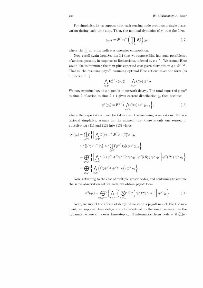
164 W. McEneaney, A. Desir
For simplicity, let us suppose that each sensing node produces a single obser-vation during each time-step. Then, the nominal dynamics of q· take the form
qk+1 = IPT⊗∨( ∏σ∈Gs
Byσ)
[qk], (12)
where the∏
notation indicates operator composition.Now, recall again from Section 3.1 that we suppose Blue has some possible set
of actions, possibly in response to Red actions, indexed by v ∈ V. We assume Bluewould like to minimize the max-plus expected cost given distribution q ∈ S⊕∨X .That is, the resulting payoff, assuming optimal Blue actions takes the form (asin Section 3.1) ∧
v∈VE⊕
∨
q [c(v, ξ)] =∧v∈V
C(v)∨ q.
We now examine how this depends on network delays. The total expected payoffat time k of action at time k + 1 given current distribution qk then becomes
ψ0(qk) = E⊕∨∧v∈V
C(v)∨ qk+1
, (13)
where the expectation must be taken over the incoming observations. For no-tational simplicity, assume for the moment that there is only one sensor, σ.Substituting (11) and (12) into (13) yields
ψ0(qk) =⊕y∈Y
∨[∧
v∈VC(v)∨ IPT⊗∨[Cyσ⊗∨qk]
∨ [(Ryσ)∨ qk]
]⊗∨⊕ζ∈X
∨p⊕∨
(y|ζ)⊗∨qζ,k
=⊕y∈Y
∨[∧
v∈VC(v)∨ IPT⊗∨[Cyσ⊗∨qk]∨ [(Ryσ)∨ qk]
]⊗∨(Ryσ)∨ qk
=⊕y∈Y
∨∧v∈V
(Cyσ⊗∨IP⊗∨C(v)
)∨ qk
.
Now, returning to the case of multiple sensor nodes, and continuing to assumethe same observation set for each, we obtain payoff form
ψ0(qk) =⊕
y∈YGs
∨∧v∈V
[( ⊗σ∈Gs
∨Cyσσ
)⊗∨IP⊗∨C(v)
]∨ qk
. (14)
Next, we model the effects of delays through this payoff model. For the mo-ment, we suppose these delays are all discretized to the same time-step as thedynamics, where k indexes time-step tk. If information from node σ ∈ Gs(α)
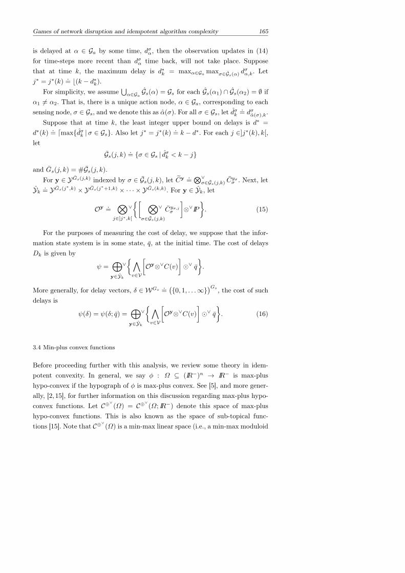
Games of network disruption and idempotent algorithm complexity 165
is delayed at α ∈ Ga by some time, dσα, then the observation updates in (14)for time-steps more recent than dσα time back, will not take place. Supposethat at time k, the maximum delay is d∗k = maxα∈Ga maxσ∈Gs(α) d
σα,k. Let
j∗ = j∗(k).= b(k − d∗k).
For simplicity, we assume⋃α∈Ga Gs(α) = Gs for each Gs(α1) ∩ Gs(α2) = ∅ if
α1 6= α2. That is, there is a unique action node, α ∈ Ga, corresponding to eachsensing node, σ ∈ Gs, and we denote this as α(σ). For all σ ∈ Gs, let dσk
.= dσα(σ),k.
Suppose that at time k, the least integer upper bound on delays is d∗ =
d∗(k).= dmaxdσk |σ ∈ Gs. Also let j∗ = j∗(k)
.= k − d∗. For each j ∈]j∗(k), k[,
let
Gs(j, k).= σ ∈ Gs | dσk < k − j
and Gs(j, k) = #Gs(j, k).For y ∈ YGs(j,k) indexed by σ ∈ Gs(j, k), let Cy .
=⊗∨
σ∈Gs(j,k) Cyσσ . Next, let
Yk.= YGs(j∗,k) × YGs(j∗+1,k) × · · · × YGs(k,k). For y ∈ Yk, let
Oy .=
⊗j∈]j∗,k[
∨[ ⊗
σ∈Gs(j,k)
∨ Cyσ,jσ
]⊗∨IP
. (15)
For the purposes of measuring the cost of delay, we suppose that the infor-mation state system is in some state, q, at the initial time. The cost of delaysDk is given by
ψ =⊕y∈Yk
∨∧v∈V
[Oy⊗∨C(v)
]∨ q
.
More generally, for delay vectors, δ ∈ WGs .=(0, 1, . . .∞
)Gs , the cost of suchdelays is
ψ(δ) = ψ(δ; q) =⊕y∈Yk
∨∧v∈V
[Oy⊗∨C(v)
]∨ q
. (16)
3.4 Min-plus convex functions
Before proceeding further with this analysis, we review some theory in idem-potent convexity. In general, we say φ : Ω ⊆ (IR−)n → IR− is max-plushypo-convex if the hypograph of φ is max-plus convex. See [5], and more gener-ally, [2,15], for further information on this discussion regarding max-plus hypo-convex functions. Let C⊕∨(Ω) = C⊕∨(Ω; IR−) denote this space of max-plushypo-convex functions. This is also known as the space of sub-topical func-tions [15]. Note that C⊕∨(Ω) is a min-max linear space (i.e., a min-max moduloid
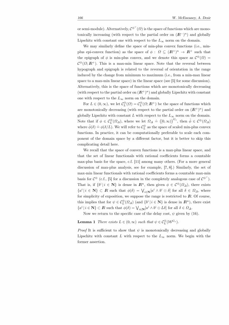
166 W. McEneaney, A. Desir
or semi-module). Alternatively, C⊕∨(Ω) is the space of functions which are mono-tonically increasing (with respect to the partial order on (IR−)n) and globallyLipschitz with constant one with respect to the L∞ norm on the domain.
We may similarly define the space of min-plus convex functions (i.e., min-plus epi-convex function) as the space of φ : Ω ⊆ (IR+)n → IR+ such thatthe epigraph of φ is min-plus convex, and we denote this space as C⊕(Ω) =
C⊕(Ω; IR+). This is a max-min linear space. Note that the reversal betweenhypograph and epigraph is related to the reversal of orientation in the rangeinduced by the change from minimum to maximum (i.e., from a min-max linearspace to a max-min linear space) in the linear space (see [5] for some discussion).Alternatively, this is the space of functions which are monotonically decreasing(with respect to the partial order on (IR+)n) and globally Lipschitz with constantone with respect to the L∞ norm on the domain.
For L ∈ (0,∞), we let C⊕L (Ω) = C⊕L (Ω; IR+) be the space of functions whichare monotonically decreasing (with respect to the partial order on (IR+)n) andglobally Lipschitz with constant L with respect to the L∞ norm on the domain.Note that if φ ∈ C⊕L (Ω∆), where we let Ω∆
.=([0,∞)
)Gs , then φ ∈ C⊕(Ω∆)
where φ(δ).= φ(δ/L). We will refer to C⊕L as the space of scaled min-plus convex
functions. In practice, it can be computationally preferable to scale each com-ponent of the domain space by a different factor, but it is better to skip thiscomplicating detail here.
We recall that the space of convex functions is a max-plus linear space, andthat the set of linear functionals with rational coefficients forms a countablemax-plus basis for the space, c.f. [11] among many others. (For a more generaldiscussion of max-plus analysis, see for example, [7, 8].) Similarly, the set ofmax-min linear functionals with rational coefficients forms a countable max-minbasis for C⊕ (c.f., [5] for a discussion in the completely analogous case of C⊕∨).That is, if bi | i ∈ N is dense in IRn, then given φ ∈ C⊕(Ω∆), there existsai | i ∈ N ⊂ IR such that φ(δ) =
∨i∈N[ai ∧ bi δ] for all δ ∈ Ω∆, where
for simplicity of exposition, we suppose the range is restricted to IR. Of course,this implies that for ψ ∈ C⊕L (Ω∆) (and bi | i ∈ N is dense in IRn), there existai | i ∈ N ⊂ IR such that φ(δ) =
∨i∈N[ai ∧ bi Lδ] for all δ ∈ Ω∆.
Now we return to the specific case of the delay cost, ψ given by (16).
Lemma 1 There exists L ∈ (0,∞) such that ψ ∈ C⊕L (WGs).
Proof It is sufficient to show that ψ is monotonically decreasing and globallyLipschitz with constant L with respect to the L∞ norm. We begin with theformer assertion.
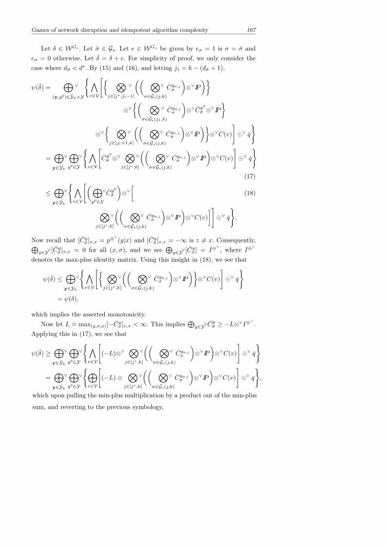
Games of network disruption and idempotent algorithm complexity 167
Let δ ∈ WGs . Let σ ∈ Gs. Let e ∈ WGs be given by eσ = 1 is σ = σ andeσ = 0 otherwise. Let δ = δ + e. For simplicity of proof, we only consider thecase where dσ < d∗. By (15) and (16), and letting j1 = k − (dσ + 1),
ψ(δ) =⊕
(y,y0)∈Yk×Y
∨
∧v∈V
[ ⊗j∈]j∗,j1−1[
∨(( ⊗
σ∈Gs(j,k)
∨ Cyσ,jσ
)⊗∨IP
)
⊗∨( ⊗
σ∈Gs(j1,k)
∨ Cyσ,jσ
)⊗∨Cy
0
σ ⊗∨IP
⊗∨ ⊗j∈]j1+1,k[
∨(( ⊗
σ∈Gs(j,k)
∨ Cyσ,jσ
)⊗∨IP
)⊗∨C(v)
]∨ q
=⊕y∈Yk
∨⊕y0∈Y
∨
∧v∈V
[Cy
0
σ ⊗∨⊗
j∈]j∗,k[
∨(( ⊗
σ∈Gs(j,k)
∨ Cyσ,jσ
)⊗∨IP
)⊗∨C(v)
]∨ q
(17)
≤⊕y∈Yk
∨
∧v∈V
[(⊕y0∈Y
∨Cy0
σ
)⊗∨[
(18)
⊗j∈]j∗,k[
∨(( ⊗
σ∈Gs(j,k)
∨ Cyσ,jσ
)⊗∨IP
)⊗∨C(v)
]]∨ q
.
Now recall that [Cyσ ]x,x = p⊕∨
(y|x) and [Cyσ ]x,z = −∞ is z 6= x. Consequently,⊕y∈Y∨[Cyσ ]x,x = 0 for all (x, σ), and we see
⊕y∈Y∨[Cyσ ] = I⊕
∨, where I⊕
∨
denotes the max-plus identity matrix. Using this insight in (18), we see that
ψ(δ) ≤⊕y∈Yk
∨
∧v∈V
[ ⊗j∈]j∗,k[
∨(( ⊗
σ∈Gs(j,k)
∨ Cyσ,jσ
)⊗∨IP
)⊗∨C(v)
]∨ q
= ψ(δ),
which implies the asserted monotonicity.Now let L .
= max(y,σ,x)[−Cyσ ]x,x < ∞. This implies⊕
y∈Y∨Cyσ ≥ −L⊗∨I⊕
∨.
Applying this in (17), we see that
ψ(δ) ≥⊕y∈Yk
∨⊕y0∈Y
∨
∧v∈V
[(−L)⊗∨
⊗j∈]j∗,k[
∨(( ⊗
σ∈Gs(j,k)
∨ Cyσ,jσ
)⊗∨IP
)⊗∨C(v)
]∨ q
=⊕y∈Yk
∨⊕y0∈Y
∨
⊕v∈V
[(−L)⊗
⊗j∈]j∗,k[
∨(( ⊗
σ∈Gs(j,k)
∨ Cyσ,jσ
)⊗∨IP
)⊗∨C(v)
]∨ q
,
which upon pulling the min-plus multiplication by a product out of the min-plus
sum, and reverting to the previous symbology,
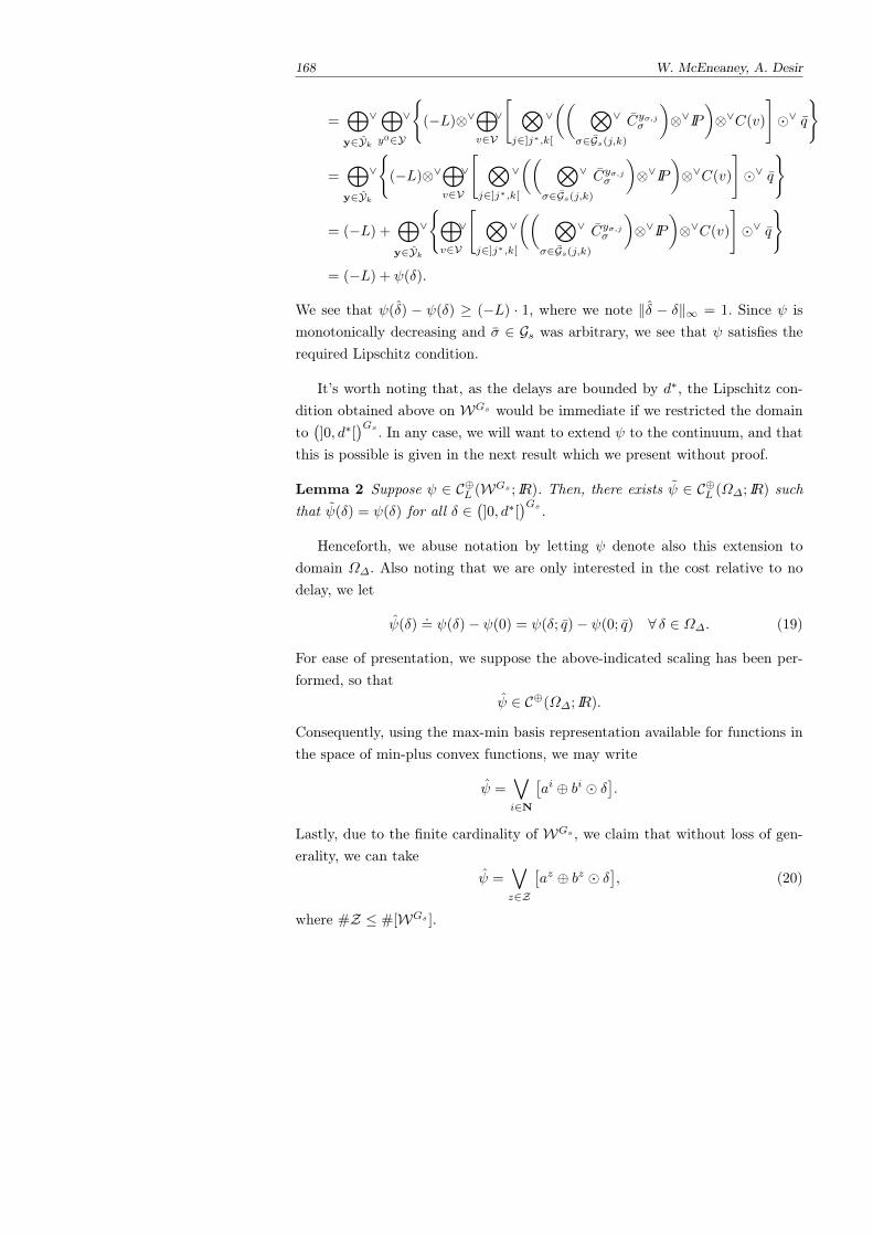
168 W. McEneaney, A. Desir
=⊕y∈Yk
∨⊕y0∈Y
∨
(−L)⊗∨
⊕v∈V
∨
[ ⊗j∈]j∗,k[
∨(( ⊗
σ∈Gs(j,k)
∨ Cyσ,jσ
)⊗∨IP
)⊗∨C(v)
]∨ q
=⊕y∈Yk
∨
(−L)⊗∨
⊕v∈V
∨
[ ⊗j∈]j∗,k[
∨(( ⊗
σ∈Gs(j,k)
∨ Cyσ,jσ
)⊗∨IP
)⊗∨C(v)
]∨ q
= (−L) +⊕y∈Yk
∨
⊕v∈V
∨
[ ⊗j∈]j∗,k[
∨(( ⊗
σ∈Gs(j,k)
∨ Cyσ,jσ
)⊗∨IP
)⊗∨C(v)
]∨ q
= (−L) + ψ(δ).
We see that ψ(δ) − ψ(δ) ≥ (−L) · 1, where we note ‖δ − δ‖∞ = 1. Since ψ ismonotonically decreasing and σ ∈ Gs was arbitrary, we see that ψ satisfies therequired Lipschitz condition.
It’s worth noting that, as the delays are bounded by d∗, the Lipschitz con-dition obtained above on WGs would be immediate if we restricted the domainto(]0, d∗[
)Gs . In any case, we will want to extend ψ to the continuum, and thatthis is possible is given in the next result which we present without proof.
Lemma 2 Suppose ψ ∈ C⊕L (WGs ; IR). Then, there exists ψ ∈ C⊕L (Ω∆; IR) suchthat ψ(δ) = ψ(δ) for all δ ∈
(]0, d∗[
)Gs .Henceforth, we abuse notation by letting ψ denote also this extension to
domain Ω∆. Also noting that we are only interested in the cost relative to nodelay, we let
ψ(δ).= ψ(δ)− ψ(0) = ψ(δ; q)− ψ(0; q) ∀ δ ∈ Ω∆. (19)
For ease of presentation, we suppose the above-indicated scaling has been per-formed, so that
ψ ∈ C⊕(Ω∆; IR).
Consequently, using the max-min basis representation available for functions inthe space of min-plus convex functions, we may write
ψ =∨i∈N
[ai ⊕ bi δ
].
Lastly, due to the finite cardinality of WGs , we claim that without loss of gen-erality, we can take
ψ =∨z∈Z
[az ⊕ bz δ
], (20)
where #Z ≤ #[WGs ].
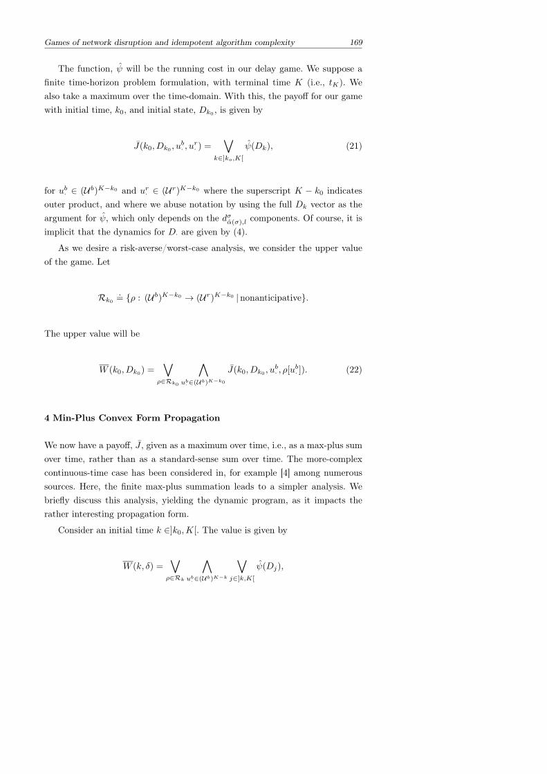
Games of network disruption and idempotent algorithm complexity 169
The function, ψ will be the running cost in our delay game. We suppose afinite time-horizon problem formulation, with terminal time K (i.e., tK). Wealso take a maximum over the time-domain. With this, the payoff for our gamewith initial time, k0, and initial state, Dk0 , is given by
J(k0, Dk0 , ub· , u
r· ) =
∨k∈]ko,K[
ψ(Dk), (21)
for ub· ∈ (Ub)K−k0 and ur· ∈ (Ur)K−k0 where the superscript K − k0 indicatesouter product, and where we abuse notation by using the full Dk vector as theargument for ψ, which only depends on the dσα(σ),l components. Of course, it isimplicit that the dynamics for D· are given by (4).
As we desire a risk-averse/worst-case analysis, we consider the upper valueof the game. Let
Rk0.= ρ : (Ub)K−k0 → (Ur)K−k0 | nonanticipative.
The upper value will be
W (k0, Dk0) =∨
ρ∈Rk0
∧ub·∈(Ub)K−k0
J(k0, Dk0 , ub· , ρ[ub· ]). (22)
4 Min-Plus Convex Form Propagation
We now have a payoff, J , given as a maximum over time, i.e., as a max-plus sumover time, rather than as a standard-sense sum over time. The more-complexcontinuous-time case has been considered in, for example [4] among numeroussources. Here, the finite max-plus summation leads to a simpler analysis. Webriefly discuss this analysis, yielding the dynamic program, as it impacts therather interesting propagation form.
Consider an initial time k ∈]k0,K[. The value is given by
W (k, δ) =∨ρ∈Rk
∧ub·∈(Ub)K−k
∨j∈]k,K[
ψ(Dj),
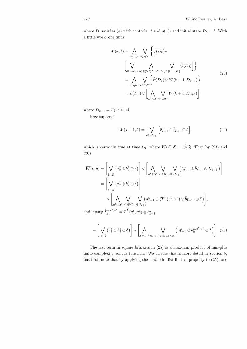
170 W. McEneaney, A. Desir
where D· satisfies (4) with controls ub· and ρ(ub· ) and initial state Dk = δ. Witha little work, one finds
W (k, δ) =∧
ubk∈Ub
∨urk∈Ur
ψ(Dk)∨
[ ∨ρ∈Rk+1
∧ub·∈(Ub)K−(k+1)
∨j∈]k+1,K[
ψ(Dj)
]
=∧
ub∈Ub
∨ur∈Ur
ψ(Dk) ∨W (k + 1, Dk+1)
= ψ(Dk) ∨[ ∧ub∈Ub
∨ur∈Ur
W (k + 1, Dk+1)
],
(23)
where Dk+1 = T (ub, ur)δ.
Now suppose
W (k + 1, δ) =∨
ω∈Ωk+1
[aωk+1 ⊕ bωk+1 δ
], (24)
which is certainly true at time tK , where W (K, δ) = ψ(δ). Then by (23) and(20)
W (k, δ) =
[∨z∈Z
(az2 ⊕ bz2 δ
)]∨
[ ∧ub∈Ub
∨ur∈Ur
∨ω∈Ωk+1
(aωk+1 ⊕ bωk+1 Dk+1
)]
=
[∨z∈Z
(az2 ⊕ bz2 δ
)]
∨
[ ∧ub∈Ub
∨ur∈Ur
∨ω∈Ωk+1
(aωk+1 ⊕ (T
T(ub, ur)⊗ bωk+1) δ
)],
and letting bω,ub,ur
k.= T
T(ub, ur)⊗ bωk+1,
=
[∨z∈Z
(az2 ⊕ bz2 δ
)]∨
[ ∧ub∈Ub
∨(ω,ur)∈Ωk+1×Ur
(aωk+1 ⊕ b
ω,ub,ur
k δ)]. (25)
The last term in square brackets in (25) is a max-min product of min-plusfinite-complexity convex functions. We discuss this in more detail in Section 5,but first, note that by applying the max-min distributive property to (25), one
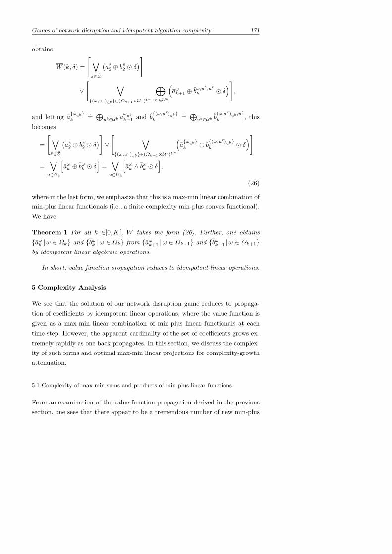
Games of network disruption and idempotent algorithm complexity 171
obtains
W (k, δ) =
[∨z∈Z
(az2 ⊕ bz2 δ
)]
∨
[ ∨(ω,ur)
ub∈(Ωk+1×Ur)Ub
⊕ub∈Ub
(aωk+1 ⊕ b
ω,ub,ur
k δ)],
and letting aωub
k.=⊕
ub∈Ub aωub
k+1 and b(ω,ur)
ub
k.=⊕
ub∈Ub b(ω,ur)
ub,ub
k , thisbecomes
=
[∨z∈Z
(az2 ⊕ bz2 δ
)]∨
[ ∨(ω,ur)
ub∈(Ωk+1×Ur)Ub
(aωub
k ⊕ b(ω,ur)ub
k δ)]
=∨ω∈Ωk
[aωk ⊕ bωk δ
]=∨ω∈Ωk
[aωk ∧ bωk δ
],
(26)
where in the last form, we emphasize that this is a max-min linear combination ofmin-plus linear functionals (i.e., a finite-complexity min-plus convex functional).We have
Theorem 1 For all k ∈]0,K[, W takes the form (26). Further, one obtainsaωk |ω ∈ Ωk and bωk |ω ∈ Ωk from aωk+1 |ω ∈ Ωk+1 and bωk+1 |ω ∈ Ωk+1by idempotent linear algebraic operations.
In short, value function propagation reduces to idempotent linear operations.
5 Complexity Analysis
We see that the solution of our network disruption game reduces to propaga-tion of coefficients by idempotent linear operations, where the value function isgiven as a max-min linear combination of min-plus linear functionals at eachtime-step. However, the apparent cardinality of the set of coefficients grows ex-tremely rapidly as one back-propagates. In this section, we discuss the complex-ity of such forms and optimal max-min linear projections for complexity-growthattenuation.
5.1 Complexity of max-min sums and products of min-plus linear functions
From an examination of the value function propagation derived in the previoussection, one sees that there appear to be a tremendous number of new min-plus
172 W. McEneaney, A. Desir
affine functions added to the value-function representation at each time-step. Inpractice, the overwhelming majority of these play no role. Typically they areeither duplicates of existing functions, or they are inactive, by which we meanthat they nowhere achieve the pointwise maximum in (26). We say a componentaffine function is strictly active if it is the unique maximizing function at somepoint. Consequently, they can be eliminated from the representation with no lossof accuracy. Within the limited space here, let us give some short synopsis of thetheory underlying max-min sums and products of min-plus affine functions.
First, we deal with finite-complexity min-plus convex functions. The generalform is
f(d) =∨j∈J
[aj ∧ bj d
]=∨j∈J
[aj ⊕ bj d
].=∨j∈J
hj(d), (27)
where J =]1, J [, d ∈ (IR+)n, aj ∈ IR+ and bj ∈ (IR+)n for all j ∈ J . LetN =]1, n[. (Here, for simplicity, we suppose the functions are defined over all of(IR+)n rather than only [0,+∞]n.) An important object with respect to eachof the min-plus affine components, hj(·), is its crux. The crux value of hj isvj
.= aj . The crux location, cj , is given component-wise as cji = vj − bji for all
i ∈]1, n[. The crux is the pair, (cj , vj). Intuitively speaking, the crux is the uniquepoint where the n+ 1 hyperplane sections which form the graph of hj intersect.The importance of the crux with regard to these expansions is evident from thefollowing simple result. Note that we suppose that duplicates have already beenremoved from representation (27) (i.e., there do not exist j 6= j such that bj = bj
and aj = aj).
Lemma 1 A min-plus affine functional is strictly active in (27) if and only ifit is strictly active at its crux location.
Proof Sufficiency is obvious, and so we only prove necessity. Suppose affine func-tion hj is strictly active. Then, there exists d ∈ IRn such that
hj(d) = aj ⊕ bj d > aj ⊕ bj d = hj(d) ∀ j ∈ J \ j. (28)
Fix any j 6= j.Suppose aj ≤ bj d. Then, by (28), aj ⊕ bj d > aj . This implies
hj(cj) = vj = aj > aj ≥ aj ⊕ bj cj = hj(cj),
which is the desired result.
Games of network disruption and idempotent algorithm complexity 173
Now instead, suppose aj > bj d. Then, by (28), aj ⊕ bj d > bj d, whichimplies
bj d > bj d. (29)
Let i ∈ N be such that
bji⊗ di = bj d. (30)
By (29) and (30), bji⊗ di > bj
i⊗ di, which implies bj
i> bj
i, and consequently,⊕
i∈N bji − b
ji < 0. This implies
hj(cj) = vj >⊕i∈N
bji + vj − bji =⊕i∈N
bji + cj
= bj cj ≥ aj ⊕ bj cj = hj(cj).
We remark that the cruxes in a finte-complexity min-plus convex functioncan also be defined geometrically, without recourse to a representation such as(27), and we do not include the details. One finds the following.
Lemma 2 The number of active affine functions in f is exactly the number ofcruxes.
We say that a finite-complexity min-plus convex functional given as (27) isin minimal form if it does not contain any inactive affine functionals. We alsonote the following useful result, and do not include the straight-forward proof.
Theorem 1 Suppose finite-complexity min-plus convex function f : (IR+)n→IR+ has exactly J cruxes, and these are C .
= (cj , vj) | j ∈ J where J =]1, J [.Let f : (IR+)n → IR+ be given by f(d) =
∨j∈J a
j ⊗ bj d, where aj = vj andbji = vj − cji for all j ∈ J and all i ∈ N . Then, f = f , and this is the uniqueminimal form.
Max-min sums of finite-complexity min-plus convex functions increase thecomplexity at most linearly, with this growth often being tempered by cruxdominance. On the other hand, in the value function propagation derivation,we had max-min products of finite-complexity min-plus convex functions. Veryinterestingly, because of the max-min distributive property, these may continueto be represented as finite-complexity min-plus convex functions. However, thecomplexity appears to grow very rapidly: With a product over K groups ofJ-complexity min-plus convex functions, the apparent complexity, purely fromexamination of the distributive property, is the cardinality of sequences of lengthK of elements of J , i.e., JK . However, there is another bound, induced by the
174 W. McEneaney, A. Desir
geometry, that can be significantly lower. There is some similarity in this discus-sion to the standard-sense finite-complexity discussion in [16]. We very brieflydescribe the results. Suppose
g(d) =∧k∈K
∨j∈J
hk,j(d) =∧k∈K
∨j∈J
[ak,j ⊕ bk,j d
]. (31)
In the one-dimensional case, n = 1, a very nice complexity bound is obtained.(Because of space limitations, we do not include a proof.)
Theorem 2 In the case of domain, IR+, the complexity of (31) is at most KJ−(K − 1), where this bound is tight.
Obviously, this can be much better than JK . Tight bounds in higher dimen-sions remain an open question. However, one known bound is (KJ)n−1, whereagain, space limitations do not allow for a proof.
5.2 Max-min projection and complexity attenuation
Regardless of complexity bounds, there is still a need for complexity-growthattenuation. For the general class of finite-complexity min-plus convex functions,we extend the results of [5]. There are two questions. First, what is the optimal(minimum error) complexity-reduction representation? Second, how does onecompute this representation? Due to space limitations, we only briefly indicatethe results.
In regard to the first question, results for finite-complexity standard-senseconvex functions were given in [12]. These results were extended to finite-complexity max-plus convex functions in [5]. In the case at hand, one triviallytransfers the results for the max-plus case to the min-plus case. Suppose one hasf(d) =
∨j∈J h
j(d) with J = #J , and wishes to find an approximation in theform g(d) =
∨m∈M hm(d) with M = #M < J . Note that as this is a pointwise
maximum, any error such that g(d) > f(d) for some d ∈ IRn cannot be correctedby the addition of more terms to g. Consequently, one seeks an approximationfrom below.
For given x ∈ IRk for some k ∈ N, w define the downward cone as D(x) =
x ∈ IRk | x x where denotes the partial order on IRk. Next, for a set ofpoints, X ⊂ IRk, we let 〈X〉 denote the convex hull of X. Then, we may definethe min-plus cornice of X as
C⊕(X) =⋃
x∈〈X〉
D(x).
Games of network disruption and idempotent algorithm complexity 175
One may show that our optimal complexity reduction problem reduces to maxi-mization of a min-plus convex, monotonically increasing function over an outer-product of cornices, where the cornices are formed from the coefficients describ-ing f . We find, that the optimal solution (also the optimal min-plus projection)is obtained by pruning the set of constituent min-plus affine functions describingf down to M elements (see [5]).
The second question regards the computational cost of this optimal projec-tion/pruning. Noting the discussion of cruxes above, the reader may be able tosee that the optimal projection may be obtained by evaluation of all of the con-stituent affine functions at each of the active cruxes, with a complexity-boundproportional to J2. Due to space limitations, we do not include the details.
6 Concluding Remarks
This paper considers a network disruption game, where the payoff derives fromthe reduced effectiveness of a player’s controls caused by information flow de-lays. We find that the problem may be formulated with a min-plus convex costand controlled min-plus linear dynamics. We also find that the solution maybe obtained purely by idempotent linear operations. Complexity growth is themost significant issue. We find that the growth is severely limited by geomet-ric considerations. We also find that complexity-growth attenuation is relativelystraight-forward as well. More generally, computations are easily instantiated(and bear some similarity to those appearing in [9] for a different problem class),although space limitations prevent inclusion of examples here.
The first author was supported in part by AFOSR.
References
1. M. Akian, “Densities of idempotent measures and large deviations”, Trans. Amer. Math.Soc., 109 (1999), 79–111.
2. G. Cohen, S. Gaubert, J.-P. Quadrat and I. Singer, Max-plus convex sets and functions,Idempotent Mathematics and Mathematical Physics, G. L. Litvinov and V. P. Maslov(Eds.), Contemporary Mathematics, Amer. Math. Soc., 377 (2005), 105–129.
3. P. Del Moral and M. Doisy, “Maslov idempotent probability calculus”, Theory Prob. Appl.,43 (1999), 562–576.
4. W.H. Fleming, H. Kaise and S.-J. Sheu, “Max-Plus Stochastic Control and Risk-Sensitivity”, Applied Math. and Optim., 62 (2010), 81–144.
5. S. Gaubert and W.M. McEneaney, “Min-max spaces and complexity reduction in min-maxexpansions”, Applied Math. and Optim., (to appear).
6. B. Heidergott, G.J. Olsder and J. van der Woude, Max-Plus at Work: Modeling andAnalysis of Synchronized Systems, Princeton Univ. Press, 2006.
7. V.N. Kolokoltsov and V.P. Maslov, Idempotent Analysis and Its Applications, Kluwer,1997.
8. G.L. Litvinov, V.P. Maslov and G.B. Shpiz, Idempotent Functional Analysis: An AlgebraicApproach, Mathematical Notes, 69 (2001), 696–729.
9. W.M. McEneaney, “Idempotent Method for Deception Games and Complexity Attenua-tion”, Proc. 2011 IFAC.
10. W.M. McEneaney, “Idempotent Method for Deception Games”, Proc. 2011 ACC, 4051–4056.
11. W.M. McEneaney, Max-Plus Methods for Nonlinear Control and Estimation, Birkhauser,Boston, 2006.
12. W.M. McEneaney, “Complexity Reduction, Cornices and Pruning”, Proc. of the Intl. Conf.on Tropical and Idempotent Mathematics, G.L. Litvinov and S.N. Sergeev (Eds.), Con-temporary Math. 495, Amer. Math. Soc. (2009), 293–303.
13. W.M. McEneaney, “Idempotent Method for Dynamic Games and Complexity Reductionin Min-Max Expansions”, Proc. IEEE CDC 2009.
14. A. Puhalskii, Large Deviations and Idempotent Probability, Chapman and Hall/CRCPress, 2001.
15. A.M. Rubinov and I. Singer, “Topical and Sub-Topical Functions, Downward Sets andAbstract Convexity”, Optimization, 50 (2001), 307–351.
16. E.D. Sontag, “VC dimension of neural networks”, Neural Networks and Machine Learning,Ed. C.M. Bishop, Springer (1998), 69–95.
William M. McEneaneyDept. of Mechanical and Aerospace Eng., University of California San Diego,San Diego, CA 92093-0411, USAE-mail: [email protected]
Antoine DesirDept. of Mechanical and Aerospace Eng., University of California San DiegoE-mail: [email protected]
Tropical and Idempotent Mathematics. Moscow, Russia, August 26–31, 2012
A minimum-weight perfect matching process forcost functions of concave type in 1D
Sergei NechaevAndrei Sobolevski
1. Preliminaries. Following R. McCann [5], we call a function w : R2 →R ∪ −∞ a cost function of concave type if for any x1, x2, y1, y2 ∈ R theinequality w(x1, y1)+w(x2, y2) ≤ w(x1, y2)+w(x2, y1) implies that the intervalsconnecting x1 to y1 and x2 to y2 are either disjoint or one of them is containedin the other.
Examples are w(x, y) = |x − y|α with 0 < α < 1 or w(x, y) = log |x − y|extended to the diagonal x = y by −∞. In fact whenever a cost function w
of concave type is spatially homogeneous and symmetric, i.e., w(x, y) = g(|x −y|), the function g : R+ → R ∪ −∞ must be strictly increasing and strictlyconcave [5].
Let now x1 < x2 < · · · < x2n be an even number of points on the real line R.Consider the complete graph K2n on these points, each of whose edges (xi, xj) isequipped with weight w(xi, xj). We look for a minimum-weight perfect matchingin the graph K2n, i.e., a set of n nonintersecting edges such that the sum of theirweights is minimal.
A bipartite version of this problem has been thoroughly treated for costs ofconcave type in the continuous setting in [5]. Similar discrete problems have alsobeen considered in the algorithmics literature for the specific case of the distance|x− y| [1, 4, 6] and for a general cost function of a concave type in [2, 3].
Call a matching nested if, for any two arcs (xi, xj) and (xi′ , xj′) that arepresent in the matching, the corresponding intervals in R are either disjoint orone of them is contained in the other.
Lemma 1 ([1, 5]) A minimum-weight matching is nested.
178 S. Nechaev, A. Sobolevski
Corollary 1 In a minimum-weight perfect matching, points with even numbersare matched to points with odd numbers.
2. Stabilization of optimal matchings. Suppose X = xi1≤i≤2n withx1 < x2 < · · · < x2n and X ′ = x′i′1≤i′≤2n′ with x′1 < x′2 < · · · < x′2n′ betwo sets such that x2n < x′1, i.e., X ′ lies to the right of X. We will refer tominimum-weight perfect matchings on X and X ′ as partial matchings and tothe minimum-weight perfect matching on X ∪X ′ as joint matching.
Call an arc (xi, xj) in a nested matching exposed if there is no arc (xi′ , xj′)
with xi, xj contained between xi′ and xj′ . We call all other arcs in a nestedmatching non-exposed or hidden. Intuitively, exposed arcs are those visible “fromabove” and hidden arcs are those covered with exposed ones.
It turns out that minimum-weight matchings enjoy a stabilization property:adding new points beside an existing point configuration does not affect thehidden arcs in the optimal matching thereon.
Theorem 1 ( [3]) Whenever an arc (xi, xj) is hidden in the partial matchingon X, it belongs to the joint optimal matching and is hidden there too.
Proof By contradiction, assume that some of hidden arcs in the partial matchingon X do not belong to the joint matching. Then there will be at least oneexposed arc (x`, xr) in the partial matching on X such that some points xi withx` < xi < xr are connected in the joint matching to points outside (x`, xr).
Indeed, if points inside every exposed arc (x`, xr) would be matched in thejoint matching only among themselves, then their matching could be withoutloss of generality taken the same as in the partial matching on X, and thereforeall hidden arcs between x` and xr would be preserved in the joint matching.
Suppose (x`, xr) is, e.g., the leftmost arc of the above kind. Denote all thepoints in the segment [x`, xr] that are connected in the joint matching to pointson the left of x` by z1 < z2 < · · · < zk; denote the opposite endpoints ofthe corresponding arcs by y1 > y2 > · · · > yk, where the inequalities followfrom the fact that the joint matching is nested. Likewise denote those pointsfrom [x`, xr] that are connected in the joint matching to points on the rightof xr by z′1 > z′2 > · · · > z′k′ and their counterparts in the joint matching byy′1 < y′2 < · · · < y′k′ .
Although k or k′ may be zero, the number k+ k′ must be positive and even.Indeed, by Corollary 1 the segment [x`, xr] contains an even number of pointsand all of them must be matched in a perfect matching; removing from the jointmatching all arcs whose ends both lie in [x`, xr], we are left with an even numberof points that are matched outside this segment.
Minimum-weight perfect matching for concave costs in 1D 179
Consider now a matching on the segment [x`, xr] that consists of the followingarcs: those arcs of the joint matching whose both ends belong to [x`, xr]; the arcs(z1, z2), . . . , (z2κ−1, z2κ), where1 κ = bk/2c; the arcs (z′2, z′1), . . . , (z′2κ′ , z′2κ′−1),where κ′ = bk′/2c; and (zk, z
′k′) if both k and k
′ are odd. Denote byW ′ the weightof this matching. It cannot be smaller than the weight W ′0 of the restriction ofthe optimal partial matching on X to [x`, xr]. For the total weight W of thejoint matching on X ∪X ′ we thus have
W ≥W −W ′ +W ′0. (1)
We now show that by a suitable sequence of uncrossings the right-hand side herecan be further reduced to a matching whose weight is strictly less than W .
Step 1. The arcs (z1, y1) and (x`, xr) are crossing, so that w(y1, z1) +w(x`, xr) > w(y1, x`) + w(z1, xr). Uncrossing these arcs strictly reduces theright-hand side of (1):
W > W −W ′ +W ′0 − w(y1, z1)− w(x`, xr) + w(y1, x`) + w(z1, xr).
Now the arcs (y2, z2) and (z1, xr) are crossing, so w(y2, z2) + w(z1, xr) −w(z1, z2) > w(y2, xr) and therefore
W > W−W ′+W ′0−w(y1, z1)−w(y2, z2)−w(x`, xr)+w(y1, x`)+w(z1, z2)+w(y2, xr).
Repeating this step κ = bk/2c times gives the inequality
W > W −W ′ +W ′0 − w(x`, xr)−∑
1≤i≤2κ
w(yi, zi)
+∑
1≤i≤κ
w(z2i−1, z2i) +∑
1≤i≤κ
w(y2i−1, y2i−2) + w(y2κ, xr),
where in the rightmost sum y0 is defined to be x`. Note that at this stage allarcs coming to points z1, z2, . . . from outside [x`, xr] are eliminated from thematching, except possibly (yk, zk) if k is odd.
Step 2. It is now clear by symmetry that a similar reduction step can beperformed on arcs going from z′1, z
′2, . . . to the right.
Step 3. If k and k′ are odd, we uncross the pair of arcs (yk, xk) and(yk−1, y
′k′−1 and finally the pair (zk, y′k′−1) and (z′k′ , y
′k′).
1 bξc is the largest integer n such that n ≤ ξ.
180 S. Nechaev, A. Sobolevski
The final estimate for W has the form
W > W −W ′ +W ′0 − w(x`, xr)−∑
1≤i≤k
w(yi, zi)−∑
1≤i′≤k′w(z′i′ , y
′i′)
+∑
1≤i≤κ
w(z2i−1, z2i) +∑
1≤i′≤κ′
w(z′2i′ , z′2i′−1) + w(zk, z
′k′) · [k, k′ are odd]
+∑
1≤i≤κ
w(y2i−1, y2i−2)+∑
1≤i′≤κ′
w(y′2i′−2, y′2i′−1)+w(yk, y
′k′) · [k, k′ are even],
(2)
where notation such as [k, k′ are odd] means 1 if k, k′ are odd and 0 otherwise.The right-hand side of (2) contains four groups of terms: first,
W −∑
1≤i≤k
w(yi, zi)−∑
1≤i′≤k′w(z′i′ , y
′i′),
corresponding to the joint matching without the arcs connecting points inside[x`, xr] to points outside this segment; second,
W ′ −∑
1≤i≤κ
w(z2i−1, z2i)−∑
1≤i′≤κ′
w(z′2i′ , z′2i′−1)− w(zk, z′k′) · [k, k′ are odd],
which comes with a negative sign and corresponds to the arcs of the jointmatching with both ends inside [x`, xr], and cancels them from the total; third,W ′0 − w(x`, xr), with positive sign, which corresponds to the hidden arcs of thepartial matching on X inside the exposed arc (x`, xr), not including the latter;and finally the terms in the last line of (2), corresponding to the arcs matchingx`, xr, and points y1, . . . , yk, y′1, . . . , y′k′ , i.e., those points outside [x`, xr] thatwere connected in the joint matching to points inside this segment.
Gathering together contributions of these four groups of terms, we observethat all negative terms cancel out and what is left corresponds to a perfectmatching with a weight strictly smaller than W , in which all arcs hidden by(x`, xr) in the partial matching on X are restored. There may still be somecrossings caused by terms of the fourth group and not involving the hiddenarcs in [x`, xr]; uncrossing them if necessary gives a nested perfect matchingwhose weight is strictly less than that of the joint matching. This contradictsthe assumption that the latter is the minimum-weight matching on X ∪ X ′.Therefore all hidden arcs in the partial matching on X (and, by symmetry,those in the partial matching on X ′) belong to the joint matching.
3. The minimum-weight matching process. For indices i, j of oppositeparity and such that i < j, letWi,j be the weight of the minimum-weight perfect
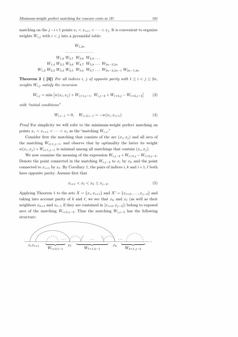
Minimum-weight perfect matching for concave costs in 1D 181
matching on the j−i+1 points xi < xi+1 < · · · < xj . It is convenient to organizeweights Wi,j with i < j into a pyramidal table:
W1,2n
. . . . . . . . . . . . . . . .
W1,6 W2,7 W3,8 W4,9 . . .
W1,4 W2,5 W3,6 W4,7 W5,8 . . . W2n−3,2n
W1,2 W2,3 W3,4 W4,5 W5,6 W6,7 . . . W2n−2,2n−1 W2n−1,2n
Theorem 2 ( [3]) For all indices i, j of opposite parity with 1 ≤ i < j ≤ 2n,weights Wi,j satisfy the recursion
Wi,j = min[w(xi, xj) +Wi+1,j−1, Wi,j−2 +Wi+2,j −Wi+2,j−2
](3)
with “initial conditions”
Wi,i−1 = 0, Wi+2,i−1 = −w(xi, xi+1). (4)
Proof For simplicity we will refer to the minimum-weight perfect matching onpoints xr < xr+1 < · · · < xs as the “matching Wr,s.”
Consider first the matching that consists of the arc (xi, xj) and all arcs ofthe matching Wi+1,j−1, and observe that by optimality the latter its weightw(xi, xj) +Wi+1,j−1 is minimal among all matchings that contain (xi, xj).
We now examine the meaning of the expression Wi,j−2 +Wi+2,j −Wi+2,j−2.Denote the point connected in the matching Wi,j−2 to xi by xk and the pointconnected to xi+1 by x`. By Corollary 1, the pairs of indices i, k and i+1, ` bothhave opposite parity. Assume first that
xi+1 < x` < xk ≤ xj−2. (5)
Applying Theorem 1 to the sets X = xi, xi+1 and X ′ = xi+2, . . . , xj−2 andtaking into account parity of k and `, we see that xk and x` (as well as theirneighbors xk+1 and x`−1 if they are contained in [xi+2, xj−2]) belong to exposedarcs of the matching Wi+2,j−2. Thus the matching Wi,j−2 has the followingstructure:
,xi xkxi+1 x`︸ ︷︷ ︸
Wi+2,`−1
· · · · · ·︸ ︷︷ ︸W`+1,k−1
· · ·︸ ︷︷ ︸Wk+1,j−2
182 S. Nechaev, A. Sobolevski
where dashed (resp., dotted) arcs correspond to those exposed arcs of the match-ing Wi+2,j−2 that belong (resp., do not belong) to Wi,j−2.
Since points x`−1 and xk+1 belong to exposed arcs in the matchingWi+2,j−2,the (possibly empty) parts of this matching that correspond to points xi+2 <
· · · < x`−1 and xk+1 < · · · < xj−2 coincide with the (possibly empty) matchingsWi+2,`−1 and Wk+1,j−2. For the same reason the (possibly empty) part of thematching Wi,j−2 supported on x`+1 < · · · < xk−1 coincides with W`+1,k−1.Therefore
Wi,j−2 = w(xi, xk) + w(xi+1, x`) +Wi+2,`−1 +W`+1,k−1 +Wk+1,j−2. (6)
Taking into account (4), observe that in the case k = i + 1 and ` = i, whichwas left out in (5), this expression still gives the correct formula Wi,j−2 =
w(xi, xi+1) +Wi+2,j−2.Now assume that in the matching Wi+1,j the point xj is connected to x`′
and the point xj−1 to xk′ . A similar argument gives
Wi+2,j =Wi+2,`′−1 +W`′+1,k′−1 +Wk′+1,j−2 + w(x`′ , xj) + w(xk′ , xj−1); (7)
in particular, if `′ = j − 1 and k′ = j, then Wi+2,j =Wi+2,j−2 + w(xj−1, xj).Suppose that xk < x`′ . Taking into account that xk, xk+1, x`′−1, and x`′ all
belong to exposed arcs in Wi+2,j−2, we can write
Wk+1,j−2 =Wk+1,`′−1 +W`′,j−2, Wi+2,`′−1 =Wi+2,k +Wk+1,`′−1 (8)
and
Wi+2,j−2 =Wi+2,k +Wk+1,`′−1 +W`′,j−2. (9)
Substituting (8) into (6) and (7) and taking into account (9), we obtain
Wi,j−2 +Wi+2,j −Wi+2,j−2 = w(xi, xk) +w(xi+1, x`) +Wi+2,`−1 +W`+1,k−1
+Wk+1,`′−1 + w(x`′ , xj) +W`′+1,k′−1 + w(xk′ , xj−1) +Wk′+1,j−2.
The right-hand side of this expression corresponds to a matching that coin-cides with Wi,j−2 on [xi, xk], with Wi+2,j−2 on [xk+1, x`′−1], and with Wi+1,j
on [x`′ , xj ]. By optimality, this matching cannot be improved on any of thesethree segments and is therefore optimal among all matchings in which xi and xjbelong to different exposed arcs.
It follows that under the assumption that xk < x`′ the expression in the right-hand side of (3) gives the minimum weight of all matchings on xi < xi+1 < · · · <xj . Moreover, the only possible candidates for the optimal matching are those
Minimum-weight perfect matching for concave costs in 1D 183
constructed above: one that corresponds to w(xi, xj) +Wi+1,j−1 and one givenby the right-hand side of the latter formula.
It remains to consider the case xk ≥ x`′ . Since xk 6= x`′ for parity reasons, itfollows that xk > x`′ ; now a construction similar to the above yields a matchingwhich corresponds to Wi,j−2 +Wi+2,j −Wi+2,j−2 and in which the arcs (xi, xk)and (x`′ , xj) are crossed. Uncrossing them leads to a matching with strictlysmaller weight, which contains the arc (xi, xj) and therefore cannot be betterthan w(xi, xj)+Wi+1,j−1. This means that (3) holds in this case too withWi,j =
w(xi, xj) +Wi+1,j−1.
We can now define a minimum-weight matching process on any locally fi-nite configuration of points (xi) in R as the recursion relations (3) and initalconditions (4) extended to all i ∈ Z.
4. The formal continuum limit. Introduce the “space” and “time” vari-ables z = h · (i+j)/2, t = τ · (j− i)/2, where h > 0 and τ > 0 are space and timemeshes, denote Wi,j = W (z, t), w(xi−1, xj+1) = w(z, t + τ), and rewrite (3) inthe form
W (z, t+ τ) = min[w(z, t+ τ)+W (z, t),W (z−h, t)+W (z+h, t)−W (z, t− τ)
].
Subtracting W (z, t+ τ) from both sides of this relation, we arrive at
minw(z, t+ τ)− [W (z, t+ τ)−W (z, t)],
W (z − h, t)− 2W (z, t) +W (z + h, t)
−W (z, t+ τ) + 2W (z, t)−W (z, t− τ)= 0,
where the term 2W (z, t) has been added and subtracted. This can be rewrittenas
min[w(z, t+ τ)− ∂tW (z, t+ τ) τ + o(τ),
∂2zW (z, t)h2 − ∂2tW (z, t) τ2 + o(h2 + τ2)]= 0.
Here ∂t (or ∂z) denotes the operator of partial derivative with respect to t (or z).Next we set h = cτ with a fixed constant c and divide the latter equal-
ity by −τ2 < 0, thus changing min to max, to get maxτ−1[∂tW − τ−1w +
o(1)], ∂2tW − c2∂2zW + o(1)= 0. Setting formally limτ↓0 τ
−1w(z, t) = ω(z, t),we finally arrive at the rescaled partial differential equation
max[∂tW − ω, 2W
]= 0, (10)
where 2W = ∂2tW − c2∂2zW is the d’Alembert wave operator. The initial con-ditions (4) are transformed into
∂tW (z, 0) = ω(z, 0), W (z, 0) = 0. (11)
Eq. (10) and initial conditions (11) constitute a formal continuous limitof (3), (4).
References
[1] A. Aggarwal, A. Bar-Noy, S. Khuller, D. Kravets, and B. Schieber, Efficient minimum costmatching using quadrangle inequality, J. Algorithms 19 (July 1995), no. 1, 116–143, DOIdoi:10.1006/jagm.1995.1030.
[2] J. Delon, J. Salomon, and A. Sobolevski, Local matching indicators for concave transportcosts, C. R. Acad. Sci. Paris, Serie I Math. 348 (Aug. 2010), no. 15–16, 901–905, DOIdoi:10.1016/j.crma.2010.07.010.
[3] , Minimum-weight perfect matching for non-intrinsic distances on the line, Feb.2011, arXiv:1102.1558.
[4] R. M. Karp and S. Y. R. Li, Two special cases of the assignment problem, Discrete Math-ematics 13 (1975), 129–142.
[5] R. J. McCann, Exact solutions to the transportation problem on the line, Proc. R. Soc. A:Math., Phys. and Eng. Sci. 455 (1999), 1341–1380.
[6] M. Werman, S. Peleg, R. Melter, and T. Y. Kong, Bipartite graph matching for points ona line or a circle, J. Algorithms 7 (1986), no. 2, 277–284.
The work was partially supported by the joint RFBR-CNRS grant 11–01–93106-a.
Sergei NechaevLPTMS, Universite Paris-Sud Centre Scientifique d’OrsayE-mail: [email protected]
Andrei SobolevskiA. A. Kharkevich Institute for Information Transmission ProblemsE-mail: [email protected]
Tropical and Idempotent Mathematics. Moscow, Russia, August 26–31, 2012
Nonlinear dynamical systems over idempotentsemirings for modelling of single agent motion inuncertain environment
Dmitry Nikolayev
1 Introduction
In the present article we introduce a new approach to modelling of single agentmotion in discrete dynamic unboundedly uncertain fully observable environmentbased on idempotent algebra. Such complex dynamical processes have been in-vestigated, algorithmically, in the artificial intelligence [1], but they were notwell understood in mathematical sense. We still do not know the underlyingequations of single greedy agent motion. An agent is called greedy if he usesgreedy strategy for decision making and chooses a suboptimal solution at eachplanning stage. The conventional control theory deals with situations withoutuncertainty [2] or uses deterministic unknown-but-bounded [3] and stochasticdescription [4] of it. We do not assume any description of uncertainty to beavailable, and to emphasize this we call it unbounded. It is very difficult tochoose appropriate mathematical tools to formalize the process of acting underunbounded uncertainty. This situation is also closely related to game theory [5],because the motion of agent in uncertain environment may be considered as adynamical game of two players, one of which may be nature itself [6]. There isa series of works about some interconnections between mean payoff games andtropical convexity [7], but they are not applicable to our case. This article showshow to obtain equations of motion in terms of idempotent semirings, which isthe the principal novelty and advantage of our approach in contrast with otherexisting approaches. We also introduce idempotent fusion semirings, i.e., idem-
186 D. Nikolayev
potent semirings with idempotent addition and fusion product playing the roleof multiplication, and construct nonlinear dynamical systems over them for mod-elling single agent’s motion in discrete unboundedly uncertain fully observableenvironment.
Idempotent mathematics is a branch of semiring theory which studies mostlysemirings with idempotent addition, a ⊕ a = a. Well-studied examples of suchalgebraic structures are Rmin and Rmax semirings, also called tropical. Rmin
is the set R ∪ +∞ equipped with addition a ⊕ b = min(a, b), multiplicationa b = a + b, zero 0 = +∞, and unity 1 = 0. Their study is motivated bymany practical applications, arising in discrete event systems, optimal schedul-ing, and modelling of synchronization problems in multiprocessor interactive sys-tems [8]. Tropical semirings and dynamical systems over them are too restrictiveto model processes of acting under unbounded uncertainty. Therefore, in thepresent article we have to develop a different approach based on a new "cate-gory" of semirings, namely, idempotent fusion semirings Fmin and Fmax, andbuild a new class of nonlinear dynamical systems over them. Notice that similaralgebraic structures have already appeared under different names in graph enu-meration problems [9, 10], automata theory [11], and formal languages [12]. Wedefine new selective addition operations a ⊕ b = lexmin(argminz∈a,b|z|) anda ⊕ b = lexmax(argmaxz∈a,b|z|) to build new one-valued idempotent semir-ings Fmin and Fmax, as opposed to the previous works, where analogous semir-ings were multi-valued and therefore inconvenient for solving game-theoretical,control-theoretical, and optimization problems.
2 Idempotent fusion semirings
Idempotent fusion semiring is the set of all finite elementary words over thealphabet of natural numbers NF|e∪χ equipped with idempotent addition a⊕b = lexmin(argminz∈a,b|z|), noncommutative multiplication, also called fusionproduct, ab = α1 . . . αkβ2 . . . βl if αk = β1 and empty set ∅ otherwise, zero 0 =
∅, and unit 1 = χ where Nk is the kth Cartesian power of the natural numbersset N, F is the Kleene operator with respect to the union ∪ and the Cartesianproduct × operations, |e is the constraint predicate restricting NF to its subsetof all words with distinct symbols, χ is a formal symbol representing the unity ofalgebraic structure, | · | is the word’s length, i.e. the number of symbols, lexmin isthe lexicographic minimum of two words a = α1 . . . αk, b = β1 . . . βl ∈ NF. Thisalgebraic structure forms a semiring if we suppose that |∅| = +∞ and |χ| = 0.Similarly, Fmax is defined with addition a ⊕ b = lexmax(argmaxz∈a,b|z|). It
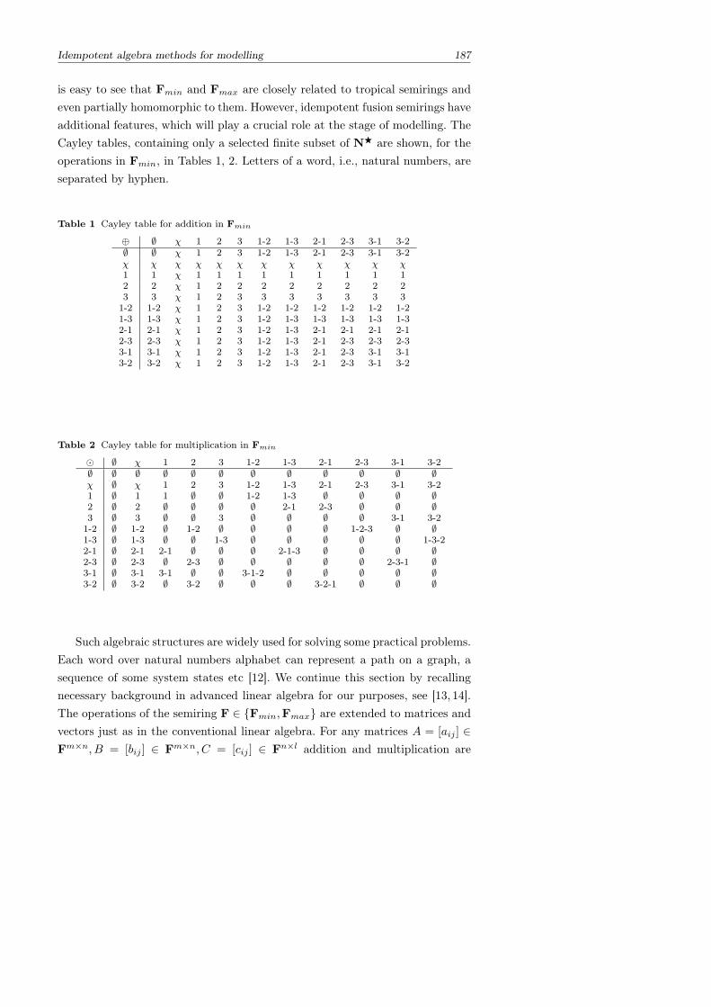
Idempotent algebra methods for modelling 187
is easy to see that Fmin and Fmax are closely related to tropical semirings andeven partially homomorphic to them. However, idempotent fusion semirings haveadditional features, which will play a crucial role at the stage of modelling. TheCayley tables, containing only a selected finite subset of NF are shown, for theoperations in Fmin, in Tables 1, 2. Letters of a word, i.e., natural numbers, areseparated by hyphen.
Table 1 Cayley table for addition in Fmin
⊕ ∅ χ 1 2 3 1-2 1-3 2-1 2-3 3-1 3-2∅ ∅ χ 1 2 3 1-2 1-3 2-1 2-3 3-1 3-2χ χ χ χ χ χ χ χ χ χ χ χ1 1 χ 1 1 1 1 1 1 1 1 12 2 χ 1 2 2 2 2 2 2 2 23 3 χ 1 2 3 3 3 3 3 3 31-2 1-2 χ 1 2 3 1-2 1-2 1-2 1-2 1-2 1-21-3 1-3 χ 1 2 3 1-2 1-3 1-3 1-3 1-3 1-32-1 2-1 χ 1 2 3 1-2 1-3 2-1 2-1 2-1 2-12-3 2-3 χ 1 2 3 1-2 1-3 2-1 2-3 2-3 2-33-1 3-1 χ 1 2 3 1-2 1-3 2-1 2-3 3-1 3-13-2 3-2 χ 1 2 3 1-2 1-3 2-1 2-3 3-1 3-2
Table 2 Cayley table for multiplication in Fmin
∅ χ 1 2 3 1-2 1-3 2-1 2-3 3-1 3-2∅ ∅ ∅ ∅ ∅ ∅ ∅ ∅ ∅ ∅ ∅ ∅χ ∅ χ 1 2 3 1-2 1-3 2-1 2-3 3-1 3-21 ∅ 1 1 ∅ ∅ 1-2 1-3 ∅ ∅ ∅ ∅2 ∅ 2 ∅ ∅ ∅ ∅ 2-1 2-3 ∅ ∅ ∅3 ∅ 3 ∅ ∅ 3 ∅ ∅ ∅ ∅ 3-1 3-21-2 ∅ 1-2 ∅ 1-2 ∅ ∅ ∅ ∅ 1-2-3 ∅ ∅1-3 ∅ 1-3 ∅ ∅ 1-3 ∅ ∅ ∅ ∅ ∅ 1-3-22-1 ∅ 2-1 2-1 ∅ ∅ ∅ 2-1-3 ∅ ∅ ∅ ∅2-3 ∅ 2-3 ∅ 2-3 ∅ ∅ ∅ ∅ ∅ 2-3-1 ∅3-1 ∅ 3-1 3-1 ∅ ∅ 3-1-2 ∅ ∅ ∅ ∅ ∅3-2 ∅ 3-2 ∅ 3-2 ∅ ∅ ∅ 3-2-1 ∅ ∅ ∅
Such algebraic structures are widely used for solving some practical problems.Each word over natural numbers alphabet can represent a path on a graph, asequence of some system states etc [12]. We continue this section by recallingnecessary background in advanced linear algebra for our purposes, see [13, 14].The operations of the semiring F ∈ Fmin,Fmax are extended to matrices andvectors just as in the conventional linear algebra. For any matrices A = [aij ] ∈Fm×n, B = [bij ] ∈ Fm×n, C = [cij ] ∈ Fn×l addition and multiplication are
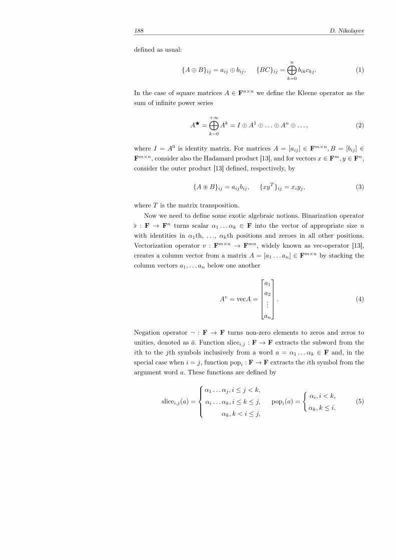
188 D. Nikolayev
defined as usual:
A⊕Bij = aij ⊕ bij , BCij =
n⊕k=0
bikckj . (1)
In the case of square matrices A ∈ Fn×n we define the Kleene operator as thesum of infinite power series
AF =
+∞⊕k=0
Ak = I ⊕A1 ⊕ . . .⊕An ⊕ . . . , (2)
where I = A0 is identity matrix. For matrices A = [aij ] ∈ Fm×n, B = [bij ] ∈Fm×n, consider also the Hadamard product [13], and for vectors x ∈ Fm, y ∈ Fn,consider the outer product [13] defined, respectively, by
A~Bij = aijbij , xyT ij = xiyj , (3)
where T is the matrix transposition.Now we need to define some exotic algebraic notions. Binarization operator
[ : F → Fn turns scalar α1 . . . αk ∈ F into the vector of appropriate size nwith identities in α1th, . . ., αkth positions and zeroes in all other positions.Vectorization operator v : Fm×n → Fmn, widely known as vec-operator [13],creates a column vector from a matrix A = [a1 . . . an] ∈ Fm×n by stacking thecolumn vectors a1, . . . an below one another
Av = vecA =
a1
a2...an
. (4)
Negation operator ¬ : F → F turns non-zero elements to zeros and zeros tounities, denoted as a. Function slicei,j : F → F extracts the subword from theith to the jth symbols inclusively from a word a = α1 . . . αk ∈ F and, in thespecial case when i = j, function popi : F→ F extracts the ith symbol from theargument word a. These functions are defined by
slicei,j(a) =
α1 . . . αj , i ≤ j < k,
αi . . . αk, i ≤ k ≤ j,
αk, k < i ≤ j,
popi(a) =
αi, i < k,
αk, k ≤ i.(5)
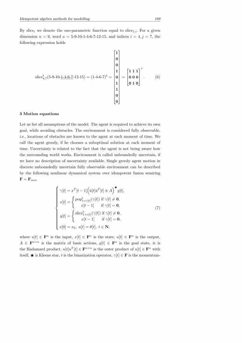
Idempotent algebra methods for modelling 189
By slicei we denote the one-parametric function equal to slice1,i. For a givendimension n = 9, word a = 5-9-10-1-4-6-7-12-15, and indices i = 4, j = 7, thefollowing expression holds
slice[4,7(5-9-10-1-4-6-7-12-15) = (1-4-6-7)[ =
1
0
0
1
0
1
1
0
0
=
1 1 1
0 0 0
0 1 0
v
. (6)
3 Motion equations
Let us list all assumptions of the model. The agent is required to achieve its owngoal, while avoiding obstacles. The environment is considered fully observable,i.e., locations of obstacles are known to the agent at each moment of time. Wecall the agent greedy, if he chooses a suboptimal solution at each moment oftime. Uncertainty is related to the fact that the agent is not being aware howthe surrounding world works. Environment is called unboundedly uncertain, ifwe have no description of uncertainty available. Single greedy agent motion indiscrete unboundedly uncertain fully observable environment can be describedby the following nonlinear dynamical system over idempotent fusion semiringF = Fmin
γ[t] = xT [t− 1](u[t]uT [t] ~A
)Fg[t],
x[t] =
pop[1+c[t](γ[t]) if γ[t] 6= 0,
x[t− 1] if γ[t] = 0,
y[t] =
slice[1+c[t](γ[t]) if γ[t] 6= 0,
x[t− 1] if γ[t] = 0,
x[0] = x0, u[t] = θ[t], t ∈ N,
(7)
where u[t] ∈ Fn is the input, x[t] ∈ Fn is the state, u[t] ∈ Fn is the output,A ∈ Fn×n is the matrix of basic actions, g[t] ∈ Fn is the goal state, ~ isthe Hadamard product, u[t]uT [t] ∈ Fn×n is the outer product of u[t] ∈ Fn withitself, F is Kleene star, [ is the binarization operator, γ[t] ∈ F is the momentum-
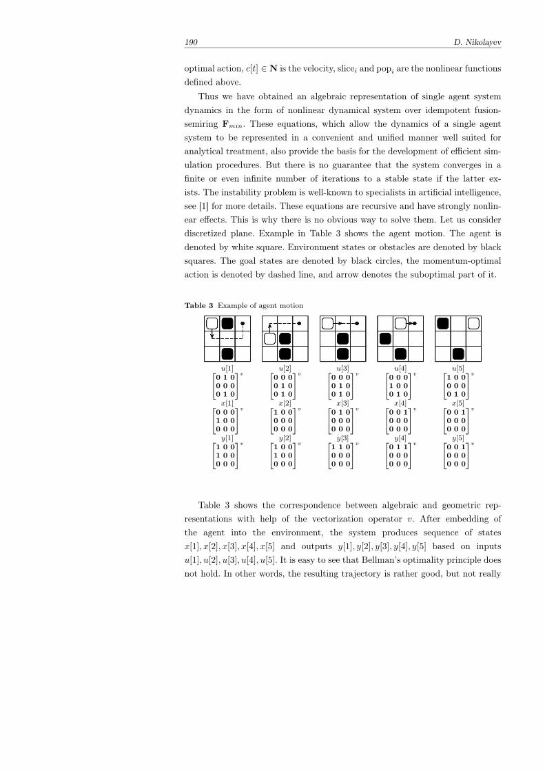
190 D. Nikolayev
optimal action, c[t] ∈ N is the velocity, slicei and popi are the nonlinear functionsdefined above.
Thus we have obtained an algebraic representation of single agent systemdynamics in the form of nonlinear dynamical system over idempotent fusion-semiring Fmin. These equations, which allow the dynamics of a single agentsystem to be represented in a convenient and unified manner well suited foranalytical treatment, also provide the basis for the development of efficient sim-ulation procedures. But there is no guarantee that the system converges in afinite or even infinite number of iterations to a stable state if the latter ex-ists. The instability problem is well-known to specialists in artificial intelligence,see [1] for more details. These equations are recursive and have strongly nonlin-ear effects. This is why there is no obvious way to solve them. Let us considerdiscretized plane. Example in Table 3 shows the agent motion. The agent isdenoted by white square. Environment states or obstacles are denoted by blacksquares. The goal states are denoted by black circles, the momentum-optimalaction is denoted by dashed line, and arrow denotes the suboptimal part of it.
Table 3 Example of agent motion
u[1] u[2] u[3] u[4] u[5]0 1 00 0 00 1 0
v 0 0 00 1 00 1 0
v 0 0 00 1 00 1 0
v 0 0 01 0 00 1 0
v 1 0 00 0 00 1 0
v
x[1] x[2] x[3] x[4] x[5]0 0 01 0 00 0 0
v 1 0 00 0 00 0 0
v 0 1 00 0 00 0 0
v 0 0 10 0 00 0 0
v 0 0 10 0 00 0 0
v
y[1] y[2] y[3] y[4] y[5]1 0 01 0 00 0 0
v 1 0 01 0 00 0 0
v 1 1 00 0 00 0 0
v 0 1 10 0 00 0 0
v 0 0 10 0 00 0 0
v
Table 3 shows the correspondence between algebraic and geometric rep-resentations with help of the vectorization operator v. After embedding ofthe agent into the environment, the system produces sequence of statesx[1], x[2], x[3], x[4], x[5] and outputs y[1], y[2], y[3], y[4], y[5] based on inputsu[1], u[2], u[3], u[4], u[5]. It is easy to see that Bellman’s optimality principle doesnot hold. In other words, the resulting trajectory is rather good, but not really
optimal. Note that this system is not asymptotically stable in general case. Sit-uations where the system does not converge to some stable state are very rare inpractice. This is why such single-agents with greedy suboptimal decision mak-ing strategy found many applications in robotics, computer graphics, and someother areas related to artificial intelligence.
References
1. S. Russell and P. Norvig Artificial Intelligence : a Modern Approach. London: PrenticeHall, 2010.
2. V.N. Kolokoltsov and V.P. Maslov Idempotent analysis and its applications. Mathematicsand its Applications, vol. 401, Dordrecht: Kluwer Academic Publishers Group, 1997.
3. L. Jaulin, M. Keiffer, O. Didrit, and E. Walter Applied Interval Analysis. London:Springer, 2007.
4. R. Tempo, G. Calafiore, and F. Dabbene Randomized Algorithms for Analysis and Controlof Uncertain Systems, London: Springer-Verlag, 2005.
5. V.N. Kolokoltsov and O.A. Malafeyev Understanding Game Theory : Introduction to theAnalysis of Many Agent Systems with Competition and Cooperation. Singapore: WorldScientific, 2010.
6. T. Bazar and G.J. Olsder Dynamic Noncooperative Game Theory: New Models and Al-gorithms. Philadelphia: Society for Industrial and Applied Mathematics, 1999.
7. X. Allamigeon, S. Gaubert, and R. Katz Tropical polar cones, hypergraph transversals,and mean payoff games. Linear algebra and its Applications, vol. 435, no. 7, 2011, 1549-1574.
8. F. Baccelli, G. Cohen, G.J. Olsder, J.-P. Quadrat Synchronization and Linearity : analgebra for discrete event systems. New York: Wiley, 1992.
9. B. Carre Graphs and Networks. London: Oxford University Press, 1979.10. M. Gondran and M. Minoux Graphs, Dioids and Semirings: New Models and Algorithms.
Heidelberg: Springer Science + Business Media, 2008.11. J. Hopcroft, R. Motwani, and J. Ullman Introduction to Automata Theory, Languages,
and Computation. Addison-Wesley, 2001.12. J.S. Golan Semirings and their applications. Dordrecht: Kluwer Academic Publishers,
1999.13. L. Hogben Handbook of Linear Algebra. London: Chapman & Hall / CRC, 2007.14. G.H. Golub and C.F. Van Loan Matrix Computations. London: John Hopkins Studies in
the Mathematical Sciences, 1996.
The work was partially supported by RFBR grant 11-07-00580-a.
Dmitry NikolayevLipetsk State Technical UniversityE-mail: [email protected]
Tropical and Idempotent Mathematics. Moscow, Russia, August 26–31, 2012
Idempotent algebra methods for modellingof hierarchical multiagent systems motion
Dmitry Nikolayev
1 Introduction
We propose a new approach to modelling of hierarchical greedy multiagent sys-tems motion based on nonlinear dynamical 2D-systems, i.e., systems with twodimensional parameter [1], over idempotent fusion semirings. Agent is calledgreedy if he uses greedy strategy for decision making and chooses a subopti-mal solution at each planning stage. We consider multiagent systems, whereall agents are greedy and have unique priorities. Since the early 1980s, motionplanning has been an intensive area of study in robotics and computational ge-ometry [2]. Most of the works in this area were focused on algorithmic motionplanning, emphasizing theoretical algorithmic analysis of the problem, seekingworst-case asymptotic bounds, new heuristic approaches to the problem, andothers [3]. However, the cooperative motion process haven’t been sufficientlywell understood in mathematical sense. We still don’t know the underlying dy-namical equations of hierarchically interacting greedy agents motion, because itis very difficult to find appropriate mathematical tools to formalize such kind ofprocesses. This situation is also closely related to control theory [4,5] and gametheory [6–8]. This article shows how to obtain equations of motion in terms ofidempotent semirings, which is the the principal novelty and advantage of ourapproach in contrast with other existing approaches.
Idempotent algebra methods for modelling 193
2 Idempotent algebra
Idempotent fusion semiring is the set of all finite elementary words over thealphabet of natural numbers NF|e∪χ equipped with idempotent addition a⊕b = lexmin(argminz∈a,b|z|), noncommutative multiplication, also called fusionproduct, ab = α1 . . . αkβ2 . . . βl if αk = β1 and empty set ∅ otherwise, zero 0 =
∅, and unit 1 = χ where Nk is the kth Cartesian power of the natural numbersset N, F is the Kleene operator with respect to the union ∪ and the Cartesianproduct × operations, |e is the constraint predicate restricting NF to it subsetof all words with distinct symbols, χ is a formal symbol representing the unit ofalgebraic structure, | · | is a word’s length, i.e. the number of symbols, lexmin isa lexicographic minimum of two words a = α1 . . . αk, b = β1 . . . βl ∈ NF. Thisalgebraic structure forms a semiring if we suppose that |∅| = +∞ and |χ| = 0.Similarly, Fmax is defined with addition a ⊕ b = lexmax(argmaxz∈a,b|z|). Itis easy to see that Fmin and Fmax are closely related to tropical semirings andeven partially homomorphic to them. However, idempotent fusion semirings haveadditional features, which at the stage of modelling will play a crucial role.
Such algebraic structures are widely used for solving some practical problems.Each word over natural numbers alphabet can represent a path on a graph, asequence of some system states [9–12]. We continue this section by recallingsome necessary background on advanced linear algebra for our purposes, see[13, 14]. The operations of the semiring F ∈ Fmin,Fmax are extended to thematrices and vectors just as in the conventional linear algebra. In the case ofsquare matrices A ∈ Fn×n, the Kleene operator is defined as the sum of infinitepower series AF = A0 ⊕ A1 ⊕ . . . ⊕ An ⊕ . . ., where A0 = I is the identitymatrix. Also for matrices A = [aij ] ∈ Fm×n, B = [bij ] ∈ Fm×n the Hadamardproduct and for vectors x ∈ Fm, y ∈ Fn the outer product are defined byfA~Bij = aijbij , xyT ij = xiyj , where T is the matrix transposition.
Now we need to define some exotic algebraic notions. Binarization operator[ : F → Fn turns scalar α1 . . . αk ∈ F into the vector of appropriate size nwith identities on α1th, . . ., αkth positions and zeroes on all other positions.Vectorization operator v : Fm×n → Fmn, widely known as vec-operator, createsa column vector from a matrix A = [a1 . . . an] ∈ Fm×n by stacking the columnvectors a1, . . . an below one another. Negation operator ¬ : F→ F turns non-zeroelements to zeros and zeros to unities, denoted as a. Function slicei,j : F → F
extracts the subword from the i-th to the j-th symbols inclusively from theargument word a = α1 . . . αk ∈ F, and function popi : F → F picks the i-thsymbol from argument word. If function slicei,j is parametrized by one parameter
194 D. Nikolayev
slicei instead of two, we assume that this parameter is j and i = 1. The listedfunctions are defined by
slicei,j(a) =
α1 . . . αj , i ≤ j < k,
αi . . . αk, i ≤ k ≤ j,
αk, k < i ≤ j,
popi(a) =
αi, i < k,
αk, k ≤ i.(1)
3 Motion equations for hierarchical multiagent systems
Prioritized motion planning for multiple agents was introduced by Erdmann andLozano-Perez [15] in 1987. It works as follows. Each of the agents is assigned aunique priority. Then in order of increasing priority, the agents are picked. Foreach picked agent a trajectory is planned, avoiding collisions with the nonstation-ary obstacles as well as the previously picked agents, which are also consideredas obstacles. This reduces the multiagent motion planning problem to the singleagent motion planning problem in a discrete unboundedly uncertain dynamicfully observable environment [7].
In the language of semiring theory, the problem is stated as follows. Given agroup of p agents and a two-dimensional discrete environment in which they canmove, let us define for each agent the matrix of basic actions A[r, t] ∈ Fn×n cov-ering all possible moves in the discrete state space, the initial state x[r, 0] ∈ Fn,the goal state g[r, t] ∈ Fn, and the speed c[r, t] ∈ N, i.e. the number of adja-cent discrete states that an agent can pass in one unit of time. Each agent isrequired to achieve its own goal state, while avoiding nonstationary obstaclesarising from nature and other agents. The shapes and moves of environmentare unconstrained and we assume no description of uncertainty to be available.Such environment is called unboundedly uncertain. The environment is consid-ered fully observable, i.e., locations of obstacles are known to every agent atevery moment of time. The group consists only of greedy agents, which in ev-ery moment choose a suboptimal solution. Uncertainty is related to the factthat agents are not being aware how the surrounding world works. Additionally,each agent has its input u[r, t] ∈ Fn (including information about environment),state x[r, t] ∈ Fn (including information about position), and output y[r, t] ∈ Fn
(including information about position and intention).A fundamental characteristic of multiagent systems is that individual agents
communicate and interact to make their actions coordinated. This is accom-plished through the exchange of messages and, to understand each other, it iscrucial that agents agree on the format and semantics of these messages. The
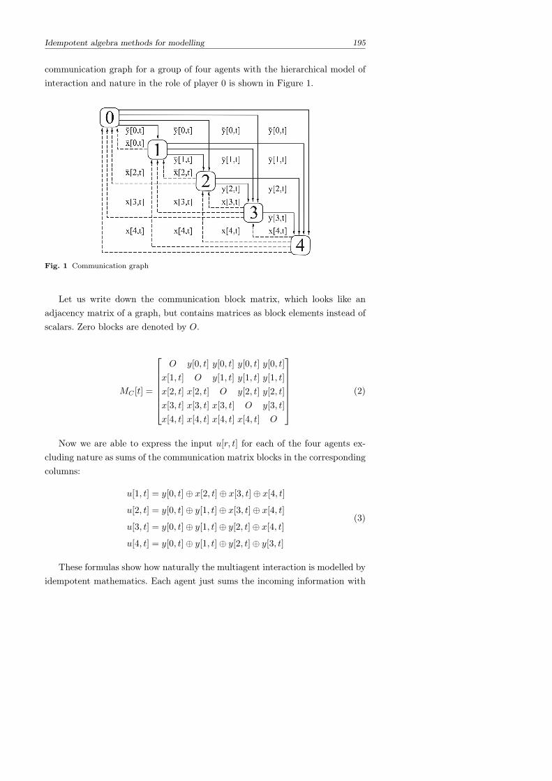
Idempotent algebra methods for modelling 195
communication graph for a group of four agents with the hierarchical model ofinteraction and nature in the role of player 0 is shown in Figure 1.
Fig. 1 Communication graph
Let us write down the communication block matrix, which looks like anadjacency matrix of a graph, but contains matrices as block elements instead ofscalars. Zero blocks are denoted by O.
MC [t] =
O y[0, t] y[0, t] y[0, t] y[0, t]
x[1, t] O y[1, t] y[1, t] y[1, t]
x[2, t] x[2, t] O y[2, t] y[2, t]
x[3, t] x[3, t] x[3, t] O y[3, t]
x[4, t] x[4, t] x[4, t] x[4, t] O
(2)
Now we are able to express the input u[r, t] for each of the four agents ex-cluding nature as sums of the communication matrix blocks in the correspondingcolumns:
u[1, t] = y[0, t]⊕ x[2, t]⊕ x[3, t]⊕ x[4, t]
u[2, t] = y[0, t]⊕ y[1, t]⊕ x[3, t]⊕ x[4, t]
u[3, t] = y[0, t]⊕ y[1, t]⊕ y[2, t]⊕ x[4, t]
u[4, t] = y[0, t]⊕ y[1, t]⊕ y[2, t]⊕ y[3, t]
(3)
These formulas show how naturally the multiagent interaction is modelled byidempotent mathematics. Each agent just sums the incoming information with
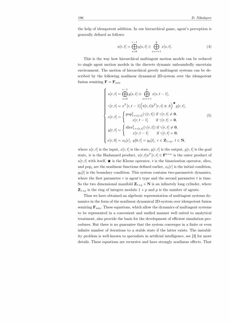
196 D. Nikolayev
the help of idempotent addition. In our hierarchical game, agent’s perception isgenerally defined as follows:
u[r, t] =
r−1⊕s=0
y[s, t]⊕p⊕
s=r+1
x[s, t]. (4)
This is the way how hierarchical multiagent motion models can be reducedto single agent motion models in the discrete dynamic unboundedly uncertainenvironment. The motion of hierarchical greedy multiagent systems can be de-scribed by the following nonlinear dynamical 2D-system over the idempotentfusion semiring F = Fmin
u[r, t] =
r−1⊕s=0
y[s, t]⊕p⊕
s=r+1
x[s, t− 1],
γ[r, t] = xT [r, t− 1](u[r, t]uT [r, t] ~A
)Fg[r, t],
x[r, t] =
pop[1+c[r,t](γ[r, t]) if γ[r, t] 6= 0,
x[r, t− 1] if γ[r, t] = 0,
y[r, t] =
slice[1+c[r,t](γ[r, t]) if γ[r, t] 6= 0,
x[r, t− 1] if γ[r, t] = 0,
x[r, 0] = x0[r], y[0, t] = y0[t], r ∈ Z1+p, t ∈ N,
(5)
where u[r, t] is the input, x[r, t] is the state, y[r, t] is the output, g[r, t] is the goalstate, ~ is the Hadamard product, u[r, t]uT [r, t] ∈ Fn×n is the outer product ofu[r, t] with itself, F is the Kleene operator, [ is the binarization operator, sliceiand popi are the nonlinear functions defined earlier, x0[r] is the initial condition,y0[t] is the boundary condition. This system contains two-parametric dynamics,where the first parameter r is agent’s type and the second parameter t is time.So the two dimensional manifold Z1+p ×N is an infinetely long cylinder, whereZ1+p is the ring of integers modulo 1 + p and p is the number of agents.
Thus we have obtained an algebraic representation of multiagent systems dy-namics in the form of the nonlinear dynamical 2D-system over idempotent fusionsemiring Fmin. These equations, which allow the dynamics of multiagent systemsto be represented in a convenient and unified manner well suited to analyticaltreatment, also provide the basis for the development of efficient simulation pro-cedures. But there is no guarantee that the system converges in a finite or eveninfinite number of iterations to a stable state if the latter exists. The instabil-ity problem is well-known to specialists in artificial intelligence, see [3] for moredetails. These equations are recursive and have strongly nonlinear effects. That
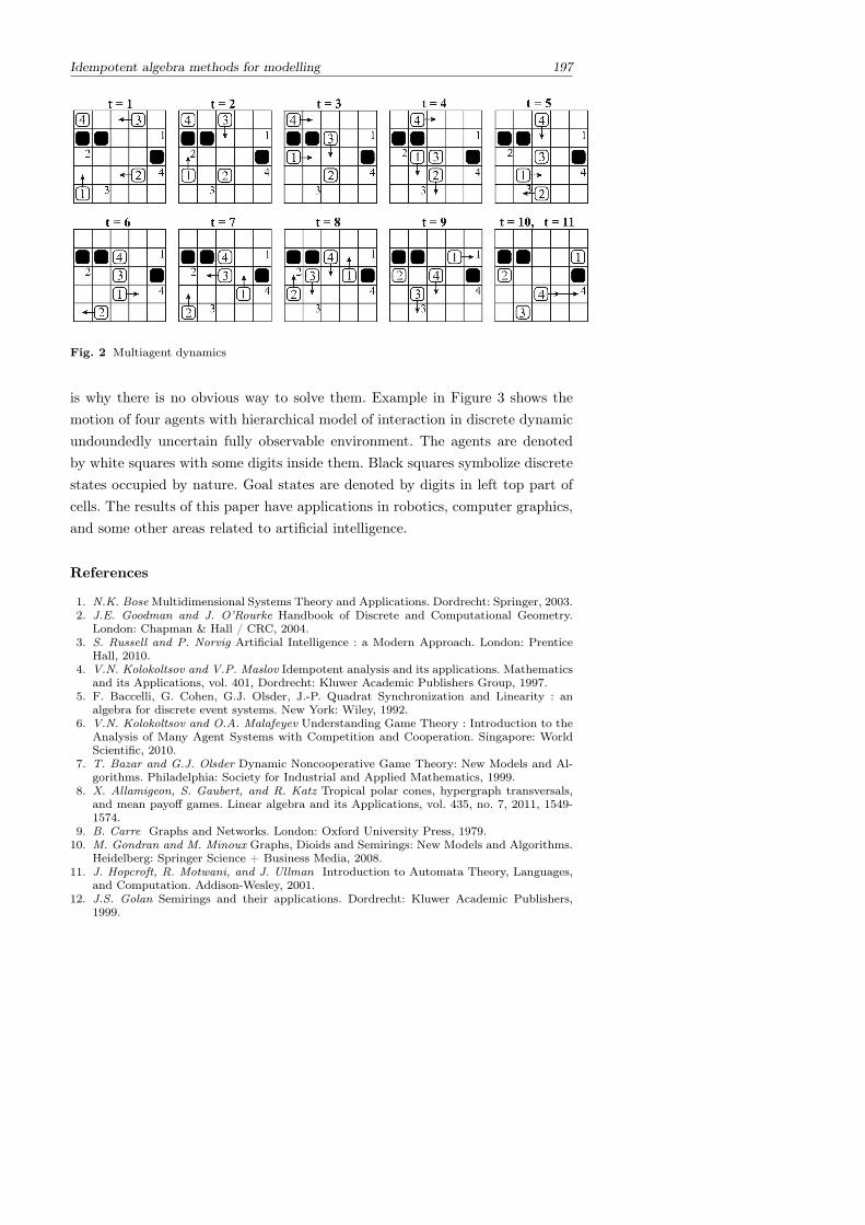
Idempotent algebra methods for modelling 197
Fig. 2 Multiagent dynamics
is why there is no obvious way to solve them. Example in Figure 3 shows themotion of four agents with hierarchical model of interaction in discrete dynamicundoundedly uncertain fully observable environment. The agents are denotedby white squares with some digits inside them. Black squares symbolize discretestates occupied by nature. Goal states are denoted by digits in left top part ofcells. The results of this paper have applications in robotics, computer graphics,and some other areas related to artificial intelligence.
References
1. N.K. Bose Multidimensional Systems Theory and Applications. Dordrecht: Springer, 2003.2. J.E. Goodman and J. O’Rourke Handbook of Discrete and Computational Geometry.
London: Chapman & Hall / CRC, 2004.3. S. Russell and P. Norvig Artificial Intelligence : a Modern Approach. London: Prentice
Hall, 2010.4. V.N. Kolokoltsov and V.P. Maslov Idempotent analysis and its applications. Mathematics
and its Applications, vol. 401, Dordrecht: Kluwer Academic Publishers Group, 1997.5. F. Baccelli, G. Cohen, G.J. Olsder, J.-P. Quadrat Synchronization and Linearity : an
algebra for discrete event systems. New York: Wiley, 1992.6. V.N. Kolokoltsov and O.A. Malafeyev Understanding Game Theory : Introduction to the
Analysis of Many Agent Systems with Competition and Cooperation. Singapore: WorldScientific, 2010.
7. T. Bazar and G.J. Olsder Dynamic Noncooperative Game Theory: New Models and Al-gorithms. Philadelphia: Society for Industrial and Applied Mathematics, 1999.
8. X. Allamigeon, S. Gaubert, and R. Katz Tropical polar cones, hypergraph transversals,and mean payoff games. Linear algebra and its Applications, vol. 435, no. 7, 2011, 1549-1574.
9. B. Carre Graphs and Networks. London: Oxford University Press, 1979.10. M. Gondran and M. Minoux Graphs, Dioids and Semirings: New Models and Algorithms.
Heidelberg: Springer Science + Business Media, 2008.11. J. Hopcroft, R. Motwani, and J. Ullman Introduction to Automata Theory, Languages,
and Computation. Addison-Wesley, 2001.12. J.S. Golan Semirings and their applications. Dordrecht: Kluwer Academic Publishers,
1999.

13. L. Hogben Handbook of Linear Algebra. London: Chapman & Hall / CRC, 2007.14. G.H. Golub and C.F. Van Loan Matrix Computations. London: John Hopkins Studies in
the Mathematical Sciences, 1996.15. M. Erdmann and T. Lozano-Perez On Multiple Moving Objects, Algorithmica, vol. 2,
1987, pp. 477 – 521.
The work was partially supported by RFBR grant 11-07-00580-a.
Dmitry NikolayevLipetsk State Technical UniversityE-mail: [email protected]
Tropical and Idempotent Mathematics. Moscow, Russia, August 26–31, 2012
The structure of max-plus hemispaces
Viorel NiticaSergeı Sergeev
1 Introduction
The work is a continuation of [5], [6] and [7], where max-plus segments, max-plus semispaces, and max-plus hyperplanes were studied. Here we describe thestructure of max-plus hemispaces. We recall thatRmax := R∪−∞ is a semifieldwith the operations ⊕ = max,⊗ = +, and that Rnmax := Rmax × ... × Rmax (n
times) is a semimodule over Rmax. For x = (x1, ..., xn), y = (y1, ..., yn) ∈ Rnmax,α ∈ Rmax define
x⊕ y := (max(x1, y1), ...,max(xn, yn)), αx := (α+ x1, ..., α+ xn). (1)
These are the basic operations in Rnmax.In analogy to the case of the real linear space, one can introduce canonically
the notion of convexity in a semimodule over a semiring (see [8], [9], [3]). Ifx, y ∈ Rnmax, the set [x, y] := (αx)⊕(βy) ∈ Rnmax|α, β ∈ Rmax, α⊕β = 0 where0 is the neutral element of ⊗ = + in Rmax, is called the max-plus segment joiningx and y. A subset G of Rnmax is said to be max-plus convex if along with any twopoints it contains the whole segment joining them, i.e., if x, y ∈ G⇒ [x, y] ⊆ G.
A (max-plus) hyperplane H in Rnmax is defined as the set of points x satisfying:
a1x1 ⊕ a2x2 ⊕ ...⊕ anxn ⊕ an+1 = b1x1 ⊕ b2x2 ⊕ ...⊕ bnxn ⊕ bn+1, (2)
with a1, ..., an, an+1, b1, ..., bn, bn+1 ∈ Rmax, where each side of (2) contains atleast one term, and where ai = bi for at least one index i. Formula (2) is calledthe equation of the hyperplane H. In contrast to the case of the usual linearspace Rn, here one needs an affine function on each side; indeed, one cannot
200 V. Nitica, S. Sergeev
simplify the equation (2) by moving one of the terms to the other side, since theoperation ⊕ does not admit an inverse operation. Among the papers investigatinghyperplanes we mention [4], [3] and [7]. If one replaces the equality sign in (2)by ≤, the set of solutions of the inequality is called max-plus halfspace. Due tothe equivalence
a ≤ b ↔ a⊕ b = b, a, b ∈ R+max,
it follows that any halfspace is also a hyperplane.Another class of convex sets in Rnmax is given by semispaces. When z ∈ Rnmax,
a subset S(z) of Rnmax is called a (max-plus) semispace at z, if it is a maximalmax-plus convex subset of Rnmax\z; a subset S of Rnmax will be called a (max-plus) semispace, if there exists z ∈ Rnmax such that S = S(z). We will refer tothe point z as the center of the semispace. It is shown in [5] and [6] that in Rnmax
there exist at most n + 1 semispaces at each point, and exactly n + 1 at eachfinite point; in particular, each max-plus convex set is contained in at least oneof those semispaces.
The structure of max-plus hemispaces in Rnmax is the main topic of the talk.A max-plus hemispace is a max-plus convex set with max-plus convex comple-mentary. The hemispaces are relevant due to Stone–Kakutani theorem: For anytwo disjoint convex sets C1, C2 ⊂ Rnmax there exists a hemispace D ⊂ Rnmax suchthat C1 ⊂ D,C2 ⊂ Rnmax \D.
Our description of hemispaces is combinatorial and geometric, and is par-tially motivated by [7], in which one can find a striking relationship betweennondegenerate max-plus hyperplanes, that is, those for which the equation (2)contains all the variables x1, . . . , xn, and max-plus semispaces. More precisely,the set corresponding to a nondegenerate max-plus hyperplane can be describedas the union of two sets: the first one is a union of complements of max-plussemispaces and the second one is the boundary of a union of complements ofmax-plus semispaces. All semispaces that appear have a common center (orapex). Moreover, any union as above coincides with a max-plus hyperplane. Ifthe hyperplane does not contain the second set above, it is also a halfspace,and this prevents the hyperplane from being a hemispace. We will show that thehemispaces are essentially halfspaces. One also needs to understand the max-plusconvex decomposition in two sets of their boundary.
2 Hemispaces in R2max
We describe the structure of hemispaces in R2max. The following theorem is [5,
Theorem 3.1].
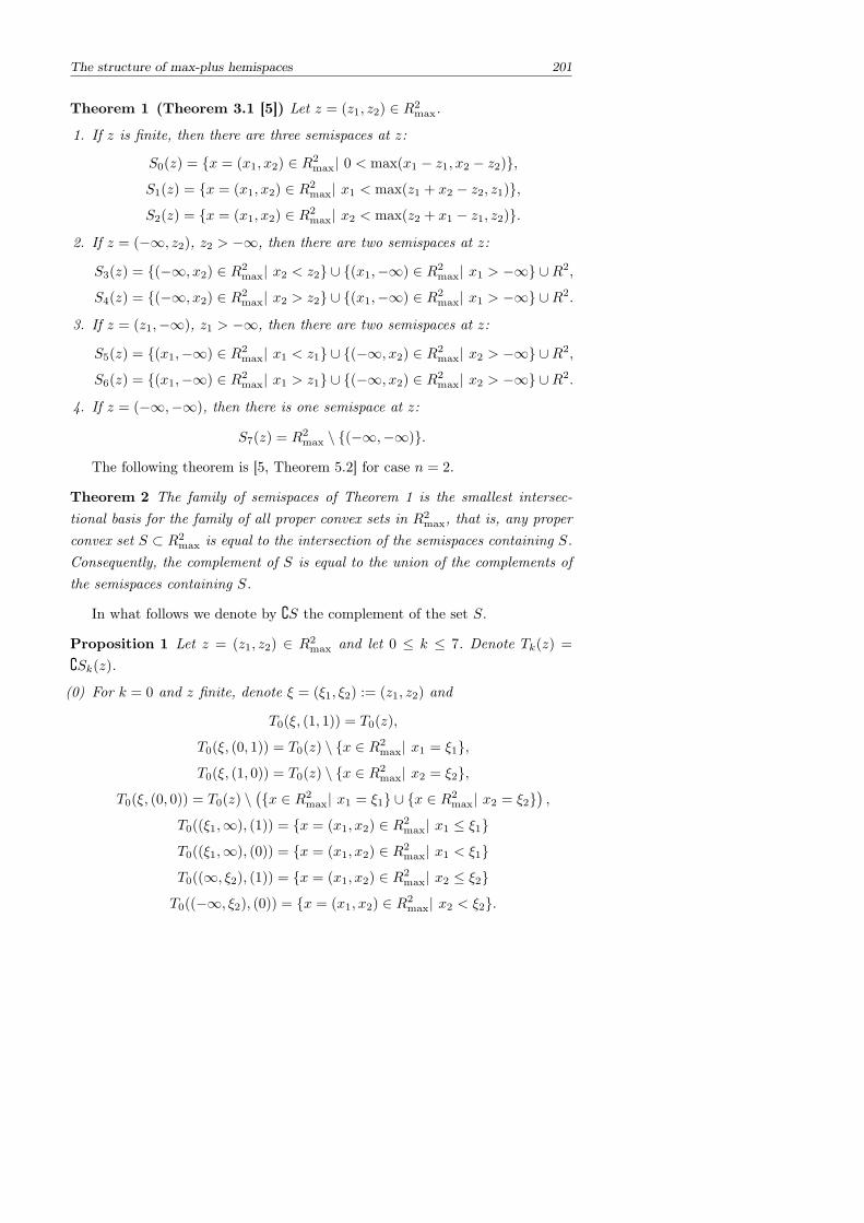
The structure of max-plus hemispaces 201
Theorem 1 (Theorem 3.1 [5]) Let z = (z1, z2) ∈ R2max.
1. If z is finite, then there are three semispaces at z:
S0(z) = x = (x1, x2) ∈ R2max| 0 < max(x1 − z1, x2 − z2),
S1(z) = x = (x1, x2) ∈ R2max| x1 < max(z1 + x2 − z2, z1),
S2(z) = x = (x1, x2) ∈ R2max| x2 < max(z2 + x1 − z1, z2).
2. If z = (−∞, z2), z2 > −∞, then there are two semispaces at z:
S3(z) = (−∞, x2) ∈ R2max| x2 < z2 ∪ (x1,−∞) ∈ R2
max| x1 > −∞ ∪R2,
S4(z) = (−∞, x2) ∈ R2max| x2 > z2 ∪ (x1,−∞) ∈ R2
max| x1 > −∞ ∪R2.
3. If z = (z1,−∞), z1 > −∞, then there are two semispaces at z:
S5(z) = (x1,−∞) ∈ R2max| x1 < z1 ∪ (−∞, x2) ∈ R2
max| x2 > −∞ ∪R2,
S6(z) = (x1,−∞) ∈ R2max| x1 > z1 ∪ (−∞, x2) ∈ R2
max| x2 > −∞ ∪R2.
4. If z = (−∞,−∞), then there is one semispace at z:
S7(z) = R2max \ (−∞,−∞).
The following theorem is [5, Theorem 5.2] for case n = 2.
Theorem 2 The family of semispaces of Theorem 1 is the smallest intersec-tional basis for the family of all proper convex sets in R2
max, that is, any properconvex set S ⊂ R2
max is equal to the intersection of the semispaces containing S.Consequently, the complement of S is equal to the union of the complements ofthe semispaces containing S.
In what follows we denote by S the complement of the set S.
Proposition 1 Let z = (z1, z2) ∈ R2max and let 0 ≤ k ≤ 7. Denote Tk(z) =
Sk(z).
(0) For k = 0 and z finite, denote ξ = (ξ1, ξ2) := (z1, z2) and
T0(ξ, (1, 1)) = T0(z),
T0(ξ, (0, 1)) = T0(z) \ x ∈ R2max| x1 = ξ1,
T0(ξ, (1, 0)) = T0(z) \ x ∈ R2max| x2 = ξ2,
T0(ξ, (0, 0)) = T0(z) \(x ∈ R2
max| x1 = ξ1 ∪ x ∈ R2max| x2 = ξ2
),
T0((ξ1,∞), (1)) = x = (x1, x2) ∈ R2max| x1 ≤ ξ1
T0((ξ1,∞), (0)) = x = (x1, x2) ∈ R2max| x1 < ξ1
T0((∞, ξ2), (1)) = x = (x1, x2) ∈ R2max| x2 ≤ ξ2
T0((−∞, ξ2), (0)) = x = (x1, x2) ∈ R2max| x2 < ξ2.
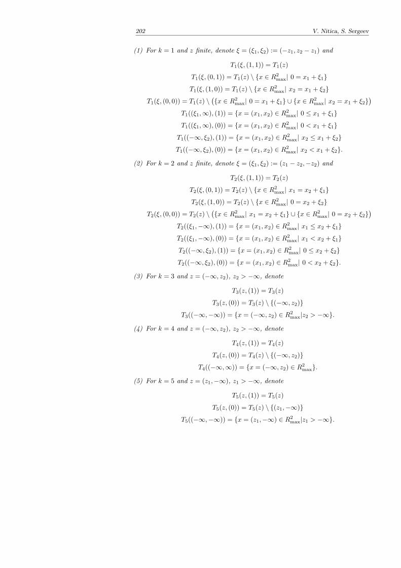
202 V. Nitica, S. Sergeev
(1) For k = 1 and z finite, denote ξ = (ξ1, ξ2) := (−z1, z2 − z1) and
T1(ξ, (1, 1)) = T1(z)
T1(ξ, (0, 1)) = T1(z) \ x ∈ R2max| 0 = x1 + ξ1
T1(ξ, (1, 0)) = T1(z) \ x ∈ R2max| x2 = x1 + ξ2
T1(ξ, (0, 0)) = T1(z) \(x ∈ R2
max| 0 = x1 + ξ1 ∪ x ∈ R2max| x2 = x1 + ξ2
)T1((ξ1,∞), (1)) = x = (x1, x2) ∈ R2
max| 0 ≤ x1 + ξ1
T1((ξ1,∞), (0)) = x = (x1, x2) ∈ R2max| 0 < x1 + ξ1
T1((−∞, ξ2), (1)) = x = (x1, x2) ∈ R2max| x2 ≤ x1 + ξ2
T1((−∞, ξ2), (0)) = x = (x1, x2) ∈ R2max| x2 < x1 + ξ2.
(2) For k = 2 and z finite, denote ξ = (ξ1, ξ2) := (z1 − z2,−z2) and
T2(ξ, (1, 1)) = T2(z)
T2(ξ, (0, 1)) = T2(z) \ x ∈ R2max| x1 = x2 + ξ1
T2(ξ, (1, 0)) = T2(z) \ x ∈ R2max| 0 = x2 + ξ2
T2(ξ, (0, 0)) = T2(z) \(x ∈ R2
max| x1 = x2 + ξ1 ∪ x ∈ R2max| 0 = x2 + ξ2
)T2((ξ1,−∞), (1)) = x = (x1, x2) ∈ R2
max| x1 ≤ x2 + ξ1
T2((ξ1,−∞), (0)) = x = (x1, x2) ∈ R2max| x1 < x2 + ξ1
T2((−∞, ξ2), (1)) = x = (x1, x2) ∈ R2max| 0 ≤ x2 + ξ2
T2((−∞, ξ2), (0)) = x = (x1, x2) ∈ R2max| 0 < x2 + ξ2.
(3) For k = 3 and z = (−∞, z2), z2 > −∞, denote
T3(z, (1)) = T3(z)
T3(z, (0)) = T3(z) \ (−∞, z2)
T3((−∞,−∞)) = x = (−∞, z2) ∈ R2max|z2 > −∞.
(4) For k = 4 and z = (−∞, z2), z2 > −∞, denote
T4(z, (1)) = T4(z)
T4(z, (0)) = T4(z) \ (−∞, z2)
T4((−∞,∞)) = x = (−∞, z2) ∈ R2max.
(5) For k = 5 and z = (z1,−∞), z1 > −∞, denote
T5(z, (1)) = T5(z)
T5(z, (0)) = T5(z) \ (z1,−∞)
T5((−∞,−∞)) = x = (z1,−∞) ∈ R2max|z1 > −∞.
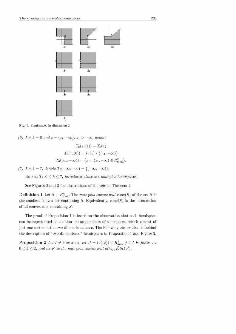
The structure of max-plus hemispaces 203
z
S0
z
S1
z
S2
z
S3
z
S4
zS5
zS6
zS7
Fig. 1 Semispaces in dimension 2
(6) For k = 6 and z = (z1,−∞), z1 > −∞, denote
T6(z, (1)) = T6(z)
T6(z, (0)) = T6(z) \ (z1,−∞)
T6((∞,−∞)) = x = (z1,−∞) ∈ R2max.
(7) For k = 7, denote T7(−∞,−∞) = (−∞,−∞).
All sets Tk, 0 ≤ k ≤ 7, introduced above are max-plus hemispaces.
See Figures 2 and 3 for illustrations of the sets in Theorem 2.
Definition 1 Let S ⊂ Rnmax. The max-plus convex hull conv(S) of the set S isthe smallest convex set containing S. Equivalently, conv(S) is the intersectionof all convex sets containing S.
The proof of Proposition 1 is based on the observation that each hemispacecan be represented as a union of complements of semispaces, which consist ofjust one sector in the two-dimensional case. The following observation is behindthe description of "two-dimensional" hemispaces in Proposition 1 and Figure 2.
Proposition 2 Let I = ∅ be a set, let zj = (zj1, zj2) ∈ R2
max, j ∈ I be finite, let0 ≤ k ≤ 2, and let F be the max-plus convex hull of ∪j∈ISk(zj).
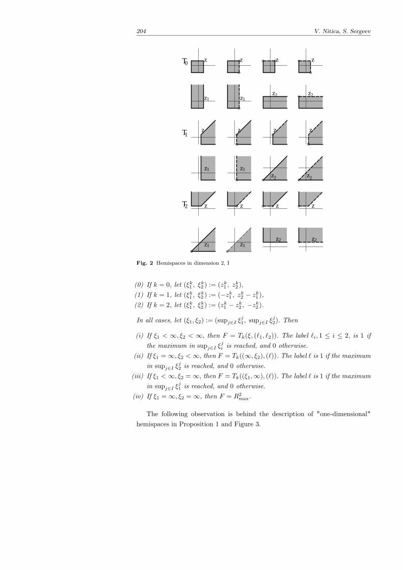
204 V. Nitica, S. Sergeev
T0z z z z
z1 z1z2 z2
T1z z z z
z1 z1z2 z2
T2 z z z z
z1 z1z2 z2
Fig. 2 Hemispaces in dimension 2, I
(0) If k = 0, let (ξk1 , ξk2 ) := (zk1 , zk2 ),
(1) If k = 1, let (ξk1 , ξk2 ) := (−zk1 , zk2 − zk1 ),(2) If k = 2, let (ξk1 , ξk2 ) := (zk1 − zk2 , −zk2 ).
In all cases, let (ξ1, ξ2) := (supj∈I ξj1, supj∈I ξ
j2). Then
(i) If ξ1 < ∞, ξ2 < ∞, then F = Tk(ξ, (ℓ1, ℓ2)). The label ℓi, 1 ≤ i ≤ 2, is 1 ifthe maximum in supj∈I ξ
ji is reached, and 0 otherwise.
(ii) If ξ1 = ∞, ξ2 <∞, then F = Tk((∞, ξ2), (ℓ)). The label ℓ is 1 if the maximumin supj∈I ξ
j2 is reached, and 0 otherwise.
(iii) If ξ1 <∞, ξ2 = ∞, then F = Tk((ξ1,∞), (ℓ)). The label ℓ is 1 if the maximumin supj∈I ξ
j1 is reached, and 0 otherwise.
(iv) If ξ1 = ∞, ξ2 = ∞, then F = R2max.
The following observation is behind the description of "one-dimensional"hemispaces in Proposition 1 and Figure 3.
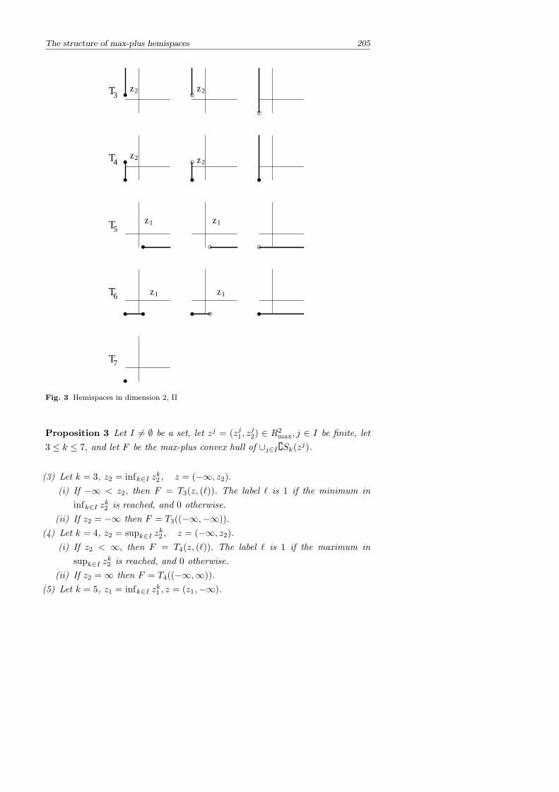
The structure of max-plus hemispaces 205
T3z2 z2
T4z2 z2
T5z1 z1
T6 z1 z1
T7
Fig. 3 Hemispaces in dimension 2, II
Proposition 3 Let I = ∅ be a set, let zj = (zj1, zj2) ∈ R2
max, j ∈ I be finite, let3 ≤ k ≤ 7, and let F be the max-plus convex hull of ∪j∈ISk(zj).
(3) Let k = 3, z2 = infk∈I zk2 , z = (−∞, z2).
(i) If −∞ < z2, then F = T3(z, (ℓ)). The label ℓ is 1 if the minimum ininfk∈I z
k2 is reached, and 0 otherwise.
(ii) If z2 = −∞ then F = T3((−∞,−∞)).(4) Let k = 4, z2 = supk∈I z
k2 , z = (−∞, z2).
(i) If z2 < ∞, then F = T4(z, (ℓ)). The label ℓ is 1 if the maximum insupk∈I z
k2 is reached, and 0 otherwise.
(ii) If z2 = ∞ then F = T4((−∞,∞)).(5) Let k = 5, z1 = infk∈I z
k1 , z = (z1,−∞).
206 V. Nitica, S. Sergeev
(i) If −∞ < z1, then F = T5(z, (ℓ)). The label ℓ is 1 if the minimum ininfk∈I z
k1 is reached, and 0 otherwise.
(ii) If z1 = −∞ then F = T5((−∞,−∞)).(6) Let k = 6, z1 = supk∈I z
k1 , z = (z1,−∞).
(i) If z1 < ∞, then F = T6(z, (ℓ)). The label ℓ is 1 if supk∈I zk1 is reached,and 0 otherwise.
(ii) If z1 = ∞ then F = T6((∞,−∞)).(7) Let k = 7. Then F = T7((−∞,−∞)) = (−∞,−∞).
Theorem 3 Let H ⊂ R2max be a hemispace. Then H is either one of the hemis-
paces listed in Proposition 1, or one of their complements.
Propositions 1 and 2 exhibit a kind of “rotational” symmetry, which is due tothe fact that each hemispace can be represented as a section of a homogeneous(or conical) hemispace, via the homogenization x 7→ (λ, λx) | λ ∈ Rmax. Tothis end, Propositions 1 and 2 could be written in the homogeneous setting,assuming z0 = 0 and redefining ξ1 and ξ2 accordingly.
General treatment of max-plus hemispaces in higher dimensions will be pre-sented in a forthcoming joint work with Ricardo D. Katz (Rosario, Argentina).
References
1. W. Briec, C.D. Horvath, Halfspaces and Hahn-Banach like properties in B-convexity andMax-Plus convexity, Pacific J. Optim. 2, 2008, 293–317.
2. W. Briec, C.D. Horvath, A.M. Rubinov, Separation in B-convexity, Pacific J. Optim. 1(2005), 13–30.
3. M. Develin, B. Sturmfels, Tropical convexity. Documenta Math., 9 (2004), 1–27.4. M. Joswig, Tropical halfspaces. Combinatorial and computational geometry, Math. Sci.
Res. Inst. Publ., vol. 52, Cambridge Univ. Press, Cambridge (2005), 409–431.5. V. Nitica, I. Singer, Max-plus convex sets and max-plus semispaces. I. Optimization 56
(2007), 171–205.6. V. Nitica, I. Singer, Max-plus convex sets and max-plus semispaces. II. Optimization 56
(2007), 293–303.7. V. Nitica, I. Singer, The structure of max-plus hyperplanes. Lin. Alg. Appl. 426 (2007),
382–414.8. K. Zimmermann, A general separation theorem in extremal algebras. Ekonom.-Mat. Ob-
zor 13 (1977), 179–201.9. K. Zimmermann, Convexity in semimodules. Ekonom.-Mat. Obzor 17 (1981), 199–213.
The work is supported by EPSRC grant RRAH15735, joint RFBR-CNRSgrant 11–01–93106-a, RFBR grant 12–01–00886-a (S. Sergeev), and SimonsFoundation grant 208729 (both authors).
Viorel NiticaUniversity of West Chester, Department of Mathematics, West Chester, PA

19383 USAE-mail: [email protected]
Sergeı SergeevUniversity of Birmingham, School of Mathematics, Birmingham, Edgbaston B152TT, UKE-mail: [email protected]
Tropical and Idempotent Mathematics. Moscow, Russia, August 26–31, 2012
Semispaces in the max-min convexity
Viorel NiticaSergeı Sergeev
1 Introduction
The max-min semiring is defined on the unit interval B = [0, 1] with arithmeticsa ⊕ b := max(a, b) and ab := min(a, b). These arithmetics can be naturallyextended to matrices and vectors leading to the max-min (fuzzy) linear algebraof [1, 4]. The max-min vectors belong to Bn, the Cartesian product of n copiesof B. The max-min interval between x, y ∈ Bn is defined as
conv(x, y) = αx⊕ (βy) | α⊕ β = 1, or
conv(x, y) = max (min(α, xi),min(β, yi)) ∀i | max (α, β) = 1.(1)
A set C ⊆ Bn is called max-min convex, if it contains, with any two pointsx, y, the interval (1) between them. For a general subset X ⊆ Bn, define itsconvex hull conv(X ) as the smallest max-min convex set containing X , i.e.,the smallest set containing X and stable under taking intervals (1).
A semispace at x ∈ Bn is defined as a maximal max-min convex set notcontaining x. A strightforward application of Zorn’s Lemma shows that if x /∈ Cand C is convex, then x can be separated from C by a semispace. It follows thatthe semispaces constitute the smallest intersectional basis of max-min convexsets (and more generally in abstract convexity).
The max-min segments and semispaces were described, respectively, in [8,11]and in [9]. In [6, 7] the authors made a further progress in the study of max-min convexity focusing on the role of semispaces. Being motivated by the Hahn-Banach separation theorems in the tropical (max-plus) convexity [12] and exten-sions to functional and abstract idempotent semimodules [2,5,13], we compared
Semispaces in the max-min convexity 209
semispaces to max-min hyperplanes in [6], and developed an interval extensionof separation by semispaces in [7]. These results are summarized below in Sec-tion 3. New results and conjectures about the Caratheodory Theorem and itscolorful extensions are given in Section 4, inspired by Gaubert and Meunier [3].
2 Description of semispaces
For any point x0 = (x01, . . . , x0n) ∈ Bn we define a family of sets
S0(x0), . . . , Sn(x
0) in Bn. These sets were shown to be semispaces in [9, Propo-sition 4.1]. Recall that x0 is called finite if it has all coordinates different fromzeros and ones. Without loss of generality we may assume that: x01 ≥ · · · ≥ x0n.
Writing this more precisely we have
x01 = · · · = x0k1 > · · · > x0k1+l1+1 = · · · = x0k1+l1+k2 > . . .
> x0k1+l1+k2+l2+1 = · · · = x0k1+l1+k2+l2+k3 > . . .
> x0k1+l1+···+kp−1+lp−1+1 = · · · = x0k1+l1+···+kp−1+lp−1+kp
> · · · > x0k1+l1+···+kp+lp(= x0n).
(2)
Let us introduce the following notations:
L0 = 0,K1 = k1, L1 = K1 + l1 = k1 + l1,
Kj = Lj−1 + kj = k1 + l1 + ...+ kj−1 + lj−1 + kj (j = 2, ..., p),
Lj = Kj + lj = k1 + l1 + ...+ kj + lj (j = 2, ..., p);
we observe that lj = 0 if and only if Kj = Lj .
We are ready to define the sets. We need to distinguish the cases when thesequence (2) ends with zeros or begin with ones, since some sets Si becomeempty in that case.
Definition 1 a) If x0 is finite, then:
S0(x0) =x ∈ Bn|xi > x0i for some 1 ≤ i ≤ n,
SKj+q(x0) =x ∈ Bn|xKj+q < x0Kj+q, or xi > x0i
for some Kj + q + 1 ≤ i ≤ n(q = 1, ..., lj ; j = 1, ..., p) if lj 6= 0,
SLj−1+q(x0) =x ∈ Bn|xLj−1+q < x0Lj−1+q, or xi > x0i
for some Kj + 1 ≤ i ≤ n
(q = 1, ..., kj ; j = 1, ..., p if k1 6= 0, or j = 2, ..., p if k1 = 0).
b) If there exists an index i ∈ 1, ..., n such that x0i = 1, but no index j suchthat x0j = 0, then the sets are S1, ..., Sn of part a).
210 V. Nitica, S. Sergeev
c) If there exists an index j ∈ 1, ..., n such that x0j = 0, but no index i suchthat x0i = 1, then the sets are S0, S1, ..., Sβ−1 of part a), where β := min1 ≤j ≤ n| x0j = 0.
d) If there exist an index i ∈ 1, ..., n such that x0i = 1, and an index j suchthat x0j = 0, then the sets are S1, ..., Sβ−1.
Proposition 1 ( [9]) For any x0 ∈ Bn the sets Si(x0), 1 ≤ i ≤ n, are max-minconvex.
3 Separation and non-separation
In the tropical convexity, all semispaces are open halfspaces expressed as solutionsets to a strict two-sided max-linear inequality. The closures of semispaces arehyperplanes. In the case of max-min convexity, hyperplane can be defined as thesolution set to
max(min(a1, x1), . . . ,min(an, xn), an+1) =
max(min(b1, x1), . . . ,min(bn, xn), bn+1).(3)
In [6] we investigated the relation between the max-min hyperplanes and theclosures of semispaces (in the usual topology), which we denote by Si(x).
Theorem 1 ( [6], Theorem 3.1) A closure of semispace is a hyperplane ifand only if it can be represented as Si(y) for some y belonging to the diagonalDn = (a, . . . , a) | a ∈ B.
This theorem shows exactly when the classical separation by hyperplanes isalways possible.
Corollary 1 ( [6], Coro. 3.3 and 3.4) Let x ∈ Bn, then any closed max-minconvex set C ⊆ Bn not containing x can be separated from x by a hyperplane ifand only if x lies on the diagonal.
A geometric idea of the proof of Theorem 1 is to construct examples of non-separation in B2 (if a point does not belong to the diagonal), and to extend itcylindrically to higher dimensions.
Below [a, c] denotes the ordinary interval on the real line b : a ≤ b ≤ c,provided a ≤ c (and possibly a = c).
In [7], we found a way to enhance separation by semispaces showing thata point can be replaced by a box, i.e., a Cartesian product of closed intervals.Namely, we investigated the separation of a box B = [x1, x1] × . . . × [xn, xn]
Semispaces in the max-min convexity 211
from a max-min convex set C ⊆ Bn, by which we mean that there exists a setS described in Definition 1, which contains C and avoids B.
Assume that x1 ≥ . . . ≥ xn and suppose that t(B) is the greatest integersuch that xt(B) ≥ xi for all 1 ≤ i ≤ t(B). We will need the following condition:
If (x1 = 1) & (yl ≥ xl, 1 ≤ l ≤ n) &
(xl < yl for some l ≤ t(B)), then y /∈ C.(4)
Note that if the box is reduced to a point and if x1 = 1, then xl = 1 for alll ≤ t(B) so that xl < yl is impossible. So (4) always holds in the case of a point.
Theorem 2 ( [7], Theorem 1) Let B = [x1, x1]×. . .×[xn, xn], and let C ⊆ Bn
be a max-min convex set avoiding B. Suppose that B and C satisfy (4). Thenthere is a set S described by Definition 1, which contains C and avoids B.
The box B can be a point and in this case condition (4) always holds. There-fore, some results on max-min semispaces [9] can be deduced from Theorem 2.The following statement is an immediate corollary of Theorem 2 and Proposition1.
Corollary 2 ( [9]) Let x ∈ Bn and C ⊆ Bn be a max-min convex set avoidingx. Then C is contained in one Si(x), 1 ≤ i ≤ n, as in Definition 1. Consequentlythese sets are indeed the family of semispaces at x.
However, separation by semispaces is impossible when B and C do not satisfy(4).
Theorem 3 ( [7], Theorem 2) Suppose that B = [x1, x1]× . . .× [xn, xn] andmax-min convex set C ⊆ Bn are such that B ∩C = ∅ but the condition (4) doesnot hold. Then there is no semispace that contains C and avoids B.
In [7] we also investigate the separation of max-min convex sets by a box,and by a box and a semispace. We show that both kinds of separation are alwayspossible n = 2, but they do not work in higher dimensions.
4. Caratheodory Theorem. Denote by Si(x0) the complement of Si(x0).As only a finite number of semispaces at a given point exist, the max-min con-vexity can be regarded as a multiorder convexity [8, 9].
Lemma 1 (Multiorder Principle) For X ⊆ Bn and x ∈ Bn, the followingare equivalent:
a) x ∈ conv(X );
212 V. Nitica, S. Sergeev
b) For all i with xi 6= 0 there exists xi ∈ X ∩ Si(x).
Like its tropical (max-plus) analogue, the max-min Caratheodory Theoremcan be easily derived either from the multiorder principle above, or from themere fact that the max-min semiring is linearly (totally) ordered.
Theorem 4 (Caratheodory) Let X ⊆ Bn and x ∈ conv(X ). Then there existx1, . . . , xn+1 ∈ X such that x ∈ conv(x1, . . . , xn+1)
Inspired by [3], let us formulate the following colourful version of Theorem 4as a conjecture.
Conjecture 1 (Colorful Caratheodory) Let C ⊆ Bn have a non-empty intersec-tion with conv(X1), . . . , conv(Xn+1), where X1, . . . ,Xn+1 are subsets of Bn. Thenthere exist xi ∈ Xi, 1 ≤ i ≤ n+ 1 such that C ∩ conv(x1, . . . , xn+1).
There are two special cases when we know that the conjecture is true: 1) whenC reduces to a point, 2) when all points in X 1, . . . ,Xn have a fixed ordering ofcoordinates, say x1 ≥ x2 ≥ . . . ≥ xn. If the ordering of coordinates is not fixed,then the sudden changes of the shape of semispaces become a major obstacle to adirect combinatorial proof. Trying to solve the problem by means of topologicalarguments, we also observed the following.
Lemma 2 (Internal Separation) Assume that the max-min convex hull ofX = x1, . . . , xn+1 ⊆ Bn has a non-empty interior. Then for any point xfrom this interior, if all coordinates of x are different, we have xi ∈ Si(x), for1 ≤ i ≤ n, up to a permutation.
The proof of the Tropical Colorful Caratheodory Theorem [3] is based on thefact that each convex hull of n points contains a set, where each point has theinternal separation property of Conjecture 2. This set can be found algebraically,see [3] or [10], and it is also non-empty when the convex hull does not haveinterior.
Conjecture 2 For each X = x1, . . . , xn+1 ⊆ Bn, the max-min convex hull of Xcontains a point x with internal separation property:
– up to a permutation, each semispace Si(x) corresponds to xi ∈ Si(x).
If Conjecture 2 holds, then so does Conjecture 1. With the assumption thateach n-tuple of points xi ∈ convX i, for i = 1, . . . , n can be approximated by
Semispaces in the max-min convexity 213
points yi with different coordinates such that conv(y1, . . . , yn) has a non-empty interior, Conjecture 1 can be proved by means of standard argumentsbased on compactness and Lemma 2.
It is generally not true that if all entries of a matrix A ∈ Bn×(n+1) aredifferent, then the max-min convex hull of the columns of A has non-emptyinterior.
For example, consider the following two matrices
A1 =
1 2 3 4
5 6 7 8
9 10 11 12
, A2 =
1 4 7 10
2 5 8 11
3 6 9 12
, (5)
The max-min convex hull of the first one has a non-empty interior, while themax-min convex hull of the second one may have only subsets of dimension two.Generalizing this example we obtained the following
Proposition 1 Let A = (aij) ∈ Bn×n+1 satisfy maxk aki ≤ mink ak,i+1. Thenconvex hull of the columns of A does not have any interior.
References
1. K. Cechlarova. On the powers of matrices in bottleneck/fuzzy algebra. Linear Alg. Appl.,246:97–111, 1996.
2. G. Cohen, S. Gaubert, J. P. Quadrat, and I. Singer. Max-plus convex sets and functions. InG. Litvinov and V. Maslov, editors, Idempotent Mathematics and Mathematical Physics,volume 377 of Contemporary Mathematics, pages 105–129. AMS, Providence, 2005. E-printhttp://www.arXiv.org/abs/math.FA/0308166.
3. S. Gaubert and F. Meunier. Caratheodory, helly and the others in the max-plus world. Discrete and Computational Geometry, 43(3):648–652, 2010. E-printhttp://www.arXiv.org/abs/0804.1361.
4. M. Gavalec. Periodicity in Extremal Algebras. Gaudeamus, Hradec Kralove, 2004.5. G. L. Litvinov, V. P. Maslov, and G. B. Shpiz. Idempotent functional analysis: An algebraic
approach. Math. Notes (Moscow), 69(5):758–797, 2001.6. V. Nitica and S. Sergeev. On hyperplanes and semispaces in max-min convex geometry.
Kybernetika, 46(3):548–557, 2010.7. V. Nitica and S. Sergeev. An interval version of separation by semispaces in max-min
convexity. Linear Alg. Appl., 435(7):1637–1648, 2011.8. V. Nitica and I. Singer. Contributions to max-min convex geometry. i: Segments. Linear
Alg. Appl., 428(7):1439–1459, 2008.9. V. Nitica and I. Singer. Contributions to max-min convex geometry. ii: Semispaces and
convex sets. Linear Alg. Appl., 428(8-9):2085–2115, 2008.10. S. Sergeev. Multiorder, Kleene stars and cyclic projectors in the geometry of max cones.
In G. L. Litvinov and S. N. Sergeev, editors, Tropical and Idempotent Mathematics, vol-ume 495 of Contemporary Mathematics, pages 317–342. AMS, Providence, 2009. E-printhttp://www.arXiv.org/abs/0807.0921.
11. S. N. Sergeev. Algorithmic complexity of a problem of idempotent convex geometry. Math.Notes (Moscow), 74(6):848–852, 2003.
12. K. Zimmermann. A general separation theorem in extremal algebras. Ekonom.-Mat. Obzor(Prague), 13:179–201, 1977.
13. K. Zimmermann. Convexity in semimodules. Ekonom.-Mat. Obzor (Prague), 17:199–213,1981.

The work is supported by EPSRC grant RRAH15735, joint RFBR-CNRSgrant 11–01–93106-a, RFBR grant 12–01–00886-a (S. Sergeev), and SimonsFoundation grant 208729 (both authors).
Viorel NiticaUniversity of West Chester, Department of Mathematics, West Chester, PA19383 USAE-mail: [email protected]
Sergeı SergeevUniversity of Birmingham, School of Mathematics, Birmingham, Edgbaston B152TT, UKE-mail: [email protected]
Tropical and Idempotent Mathematics. Moscow, Russia, August 26–31, 2012
Spectral approach to composition formulas
Michael Pevzner
Abstract We shall discuss an alternative approach to composition formulas(*-products) of quantized operators based on the representation theory ofunderlying Lie groups. Two examples, leading to interactions with numbertheory, will be presented.
1 Weyl quantization
The Weyl symbolic calculus gives a rigorous mathematical framework for thequantization procedure. It defines a correspondence that associates to a function(classical observable) S = S(x, ξ) of n + n variables, lying in S(Rn × Rn) ,the operator (quantum observable) Q(S) , called the operator with symbol S ,defined by the equation:
(Q(S)u)(x) = ~−n∫Rn×Rn
S(x+ y
2, η) e
2iπ~ 〈x−y, η〉 u(y) dy dη . (1)
Such a linear operator extends as a continuous operator from S ′(Rn) to S(Rn)
while, in the case when S ∈ S ′(Rn×Rn) , one can still define Q(S) as a linearoperator from S(Rn) to S ′(Rn) ; also, Q sets up an isometry from L2(Rn ×Rn) onto the space of Hilbert-Schmidt operators on L2(Rn) . The compositionS1 #S2 of two symbols, lying for instance in S(Rn × Rn) , is defined by theformula
Q(S1)Q(S2) = Q(S1 #S2) , (2)
216 M. Pevzner
where the left-hand side denotes the usual composition of operators. The mainconcern of this note is to compare two different approaches to the analysis of the]-product: the asymptotic and spectral ones.
The celebrated deformation quantization method developed in [1] suggeststo avoid the Heisenberg formulation of Quantum mechanics and proposes toconsider instead a quantized mechanical system as a “deformation" or a “pertur-bation" of the classical one.
According to this theory one should interpret quantum observables Q(f) asformal power series in the Planck’s constant ~ on the phase space constructedin such a way that letting ~ tend to zero one should recover the correspondingclassical observable f . The algebraic structure underlying the quantization mapQ, i.e. the way that the composition of operators Q(f) is reflected on the levelof their symbols f , and mechanical data, encoded by the Poisson bracket on thephase space, should also be respected.
In other words one should interpret the quantization procedure as a con-struction of an associative multiplication law on the space of formal power seriesin ~ that would ”deform" the usual point-wise product of functions, say f andg, in the ”direction" of the Poisson bracket :
f]g = f · g +~2f, g+ ...+
~n!Bn(f, g) + ..., (3)
where Bn’s with n > 1 stand for suitable bi-differential operators determined bythe associativity condition.
At a first glance such a requirement might look extravagant but the formula(3) may be derived from the asymptotic expansion with respect to ~ of thecomposition of two operators within Weyl calculus (1). In fact, let Λ be thecanonical Poisson structure on R2n given by Λ =
∑Λij∂i∧∂j , with Λij = −Λji ∈
0,±1. Then the composition of operators with symbols f and g respectivelygives rise to a non-commutative product f]g defined by:
Q(f) Q(g) = Q(f]g).
Naively, a composition formula for a quantization map Q is a (not necessarilyunique) expression for f]g involving f, and g.
The best known composition formula for the Weyl calculus, usually calledMoyal product, depends on the Poisson structure Λ and is given by:
f]g (z) = exp(iπ~Λrs∂xr∂ys)(f(x)g(y))|x=y=z = f · g + iπ~f, g+ ...
Spectral approach to composition formulas 217
On the other hand it turns out that the above composition formula may alsobe understood by use of the spectral theory of appropriate invariant differentialoperators.
Let us observe that the formula (1) actually defines a representation of theconvolution algebra L1(H2n+1) of the Heisenberg group H2n+1. Indeed, the im-age of the Heisenberg representation is the group of unitary transformationsexp (2iπ (〈η, q〉 − 〈y, p〉 − t)) of L2(Rn) , as made meaningful by Stone’s the-orem, where the j-th component of the vector q = (q1, . . . , qn) is the mul-tiplication by the j-th coordinate xj , p = (p1, . . . , pn) with pj = 1
2iπ∂∂xj
,and y, η ∈ Rn , t ∈ R . Introducing on (Rn × Rn)2 the symplectic form [ , ]
associated with the canonical Poisson structure Λ, which we can write as
[(x, ξ) , (y, η)] = −〈x, η〉+ 〈y, ξ〉 , (4)
let us use on Rn ×Rn the symplectic Fourier transformation F defined by theequation
(F S)(X) =
∫Rn×Rn
S(Y ) e−2iπ [X,Y ] dY , (5)
which commutes with all symplectic linear transformations of the variable inRn × Rn . Another, fully equivalent, way to define the Weyl calculus (1) is bymeans of the equation
Q(S) = ~−n∫Rn×Rn
(F S)(y, η) exp (2iπ
~(〈η, q〉 − 〈y, p〉)) dy dη . (6)
In the sequel, in order to make the presentation lighter we normalize the Planckconstant by ~ = 1.
The correspondence (1) has two types of symmetries. The first covariancerule of the Weyl calculus is the observation that
exp (2iπ (〈η, q〉 − 〈y, p〉)) Q(S) exp (−2iπ (〈η, q〉 − 〈y, p〉))
= Q((x, ξ) 7→ S(x− y, ξ − η)) . (7)
One way to emphasize this action on symbols of the group of translations of R2n
is to decompose in a systematic way the space of symbols L2(R2n) with respectto this action. Now, the operators which commute with it are just the partial dif-ferential operators with constant coefficients: the generalized joint eigenfunctionsof these are exactly the exponentials X = (x, ξ) 7→ e2iπ [A,X] with A ∈ R2n ,and the sought-after decomposition of a symbol is provided by the symplecticFourier transformation. On the other hand, if A = (y, η) , the operator withsymbol e2iπ [A,X] is none other than the operator exp (2iπ (〈η, q〉 − 〈y, p〉)) , so
218 M. Pevzner
that Heisenberg’s commutation relation, expressed in Weyl’s exponential version,takes the form
e2iπ [A1, X] # e2iπ [A2, X] = eiπ [A1, A2] e2iπ [A1+A2, X] . (8)
Let us recall some consequences of this relation. First, one has (say, whenS1 and S2 lie in S(R2n)), using (6), the integral composition formula
(S1 #S2)(X) = 22n∫R2n×R2n
S1(Y )S2(Z) e−4iπ [Y−X,Z−X] dY dZ (9)
or (a fully equivalent one)
(S1 #S2)(X) = [ exp(iπL) (S1(Y )S2(Z)) ] (Y = Z = X) (10)
with (setting Y = (y, η), Z = (z, ζ))
iπL =1
4iπ
n∑j=1
(− ∂2
∂yj ∂ζj+
∂2
∂zj ∂ηj
). (11)
Expanding the exponential into a series, one obtains the Moyal formula:
(S1 #S2)(x, ξ)
=∑ (−1)|α|
α !β !
(1
4iπ
)|α|+|β| (∂
∂x
)α (∂
∂ξ
)βS1(x, ξ)
(∂
∂x
)β (∂
∂ξ
)αS2(x, ξ) .
(12)
This formula is an exact one in the case when the two operators under con-sideration are differential operators, which means exactly that their symbols(of course, not in S(R2n)) are polynomials with respect to the variablesξ , with coefficients depending on x in a smooth, but otherwise fairly arbi-trary way; it is also exact when one of the two symbols is a polynomial in (x, ξ) .
As it turns out, this version of the composition formula is the only universallyknown one. Indeed, it has considerable importance in applications of pseudod-ifferential analysis to partial differential equations: classes of symbols for whichthe above formula, without being an exact one, still has some asymptotic value,provide a good proportion of the auxiliary operators needed for the solution ofP.D.E. problems.
Our derivation of (9) was obtained as the result of pairing the concept ofsharp composition of symbols with the decomposition of symbols according tothe action by translations of the group R2n : the success of this point of viewwas essentially dependent on the fact that this action is an ingredient of the
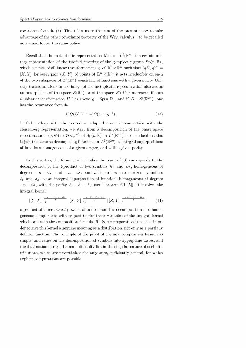
Spectral approach to composition formulas 219
covariance formula (7). This takes us to the aim of the present note: to takeadvantage of the other covariance property of the Weyl calculus – to be recallednow – and follow the same policy.
Recall that the metaplectic representation Met on L2(Rn) is a certain uni-tary representation of the twofold covering of the symplectic group Sp(n,R) ,which consists of all linear transformations g of Rn×Rn such that [gX, gY ] =
[X, Y ] for every pair (X, Y ) of points of Rn × Rn : it acts irreducibly on eachof the two subspaces of L2(Rn) consisting of functions with a given parity. Uni-tary transformations in the image of the metaplectic representation also act asautomorphisms of the space S(Rn) or of the space S ′(Rn) : moreover, if sucha unitary transformation U lies above g ∈ Sp(n,R) , and if S ∈ S ′(R2n) , onehas the covariance formula
U Q(S)U−1 = Q(S g−1) . (13)
In full analogy with the procedure adopted above in connection with theHeisenberg representation, we start from a decomposition of the phase spacerepresentation (g, S) 7→ S g−1 of Sp(n,R) in L2(R2n) into irreducibles: thisis just the same as decomposing functions in L2(R2n) as integral superpositionsof functions homogeneous of a given degree, and with a given parity.
In this setting the formula which takes the place of (8) corresponds to thedecomposition of the ]-product of two symbols h1 and h2 , homogeneous ofdegrees −n − iλ1 and −n − iλ2 and with parities characterized by indicesδ1 and δ2 , as an integral superposition of functions homogeneous of degrees−n − iλ , with the parity δ ≡ δ1 + δ2 (see Theorem 6.1 [5]). It involves theintegral kernel
| [Y, X] |−n−iλ+iλ1−iλ2
2ε2 | [X, Z] |
−n−iλ−iλ1+iλ22
ε1 | [Z, Y ] |−n+iλ+iλ1+iλ2
2ε , (14)
a product of three signed powers, obtained from the decomposition into homo-geneous components with respect to the three variables of the integral kernelwhich occurs in the composition formula (9). Some preparation is needed in or-der to give this kernel a genuine meaning as a distribution, not only as a partiallydefined function. The principle of the proof of the new composition formula issimple, and relies on the decomposition of symbols into hyperplane waves, andthe dual notion of rays. Its main difficulty lies in the singular nature of such dis-tributions, which are nevertheless the only ones, sufficiently general, for whichexplicit computations are possible.
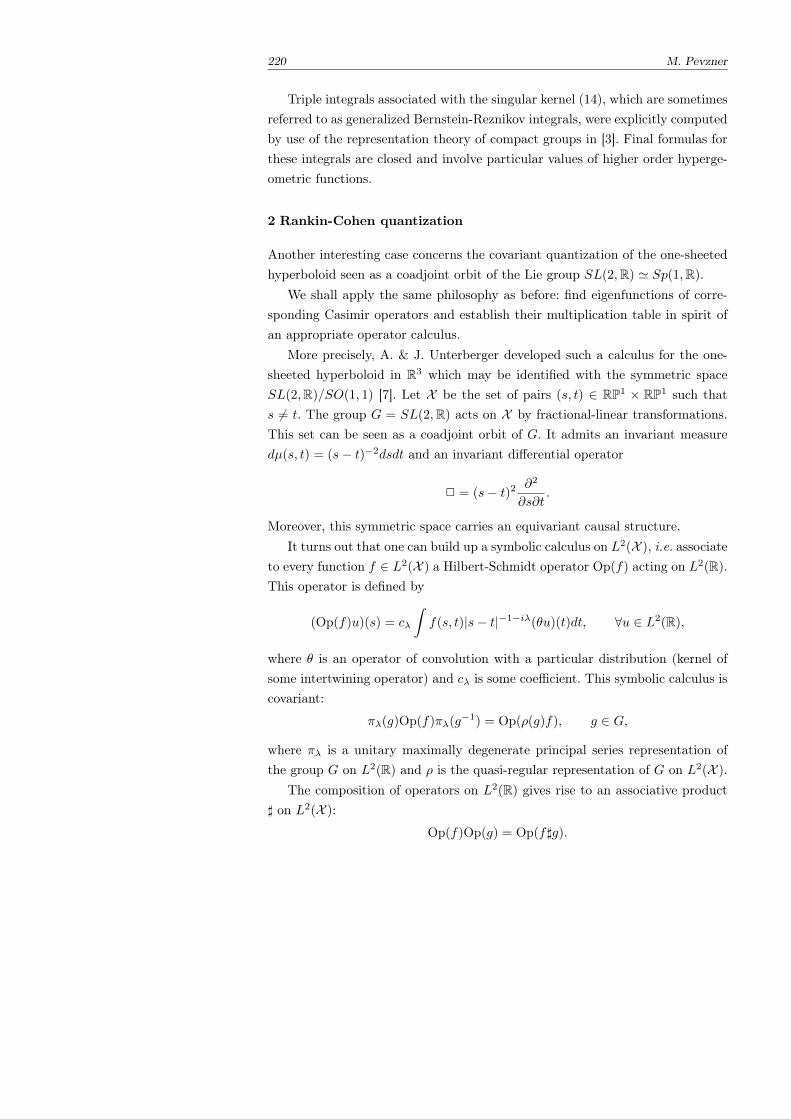
220 M. Pevzner
Triple integrals associated with the singular kernel (14), which are sometimesreferred to as generalized Bernstein-Reznikov integrals, were explicitly computedby use of the representation theory of compact groups in [3]. Final formulas forthese integrals are closed and involve particular values of higher order hyperge-ometric functions.
2 Rankin-Cohen quantization
Another interesting case concerns the covariant quantization of the one-sheetedhyperboloid seen as a coadjoint orbit of the Lie group SL(2,R) ' Sp(1,R).
We shall apply the same philosophy as before: find eigenfunctions of corre-sponding Casimir operators and establish their multiplication table in spirit ofan appropriate operator calculus.
More precisely, A. & J. Unterberger developed such a calculus for the one-sheeted hyperboloid in R3 which may be identified with the symmetric spaceSL(2,R)/SO(1, 1) [7]. Let X be the set of pairs (s, t) ∈ RP1 × RP1 such thats 6= t. The group G = SL(2,R) acts on X by fractional-linear transformations.This set can be seen as a coadjoint orbit of G. It admits an invariant measuredµ(s, t) = (s− t)−2dsdt and an invariant differential operator
2 = (s− t)2 ∂2
∂s∂t.
Moreover, this symmetric space carries an equivariant causal structure.It turns out that one can build up a symbolic calculus on L2(X ), i.e. associate
to every function f ∈ L2(X ) a Hilbert-Schmidt operator Op(f) acting on L2(R).This operator is defined by
(Op(f)u)(s) = cλ
∫f(s, t)|s− t|−1−iλ(θu)(t)dt, ∀u ∈ L2(R),
where θ is an operator of convolution with a particular distribution (kernel ofsome intertwining operator) and cλ is some coefficient. This symbolic calculus iscovariant:
πλ(g)Op(f)πλ(g−1) = Op(ρ(g)f), g ∈ G,
where πλ is a unitary maximally degenerate principal series representation ofthe group G on L2(R) and ρ is the quasi-regular representation of G on L2(X ).
The composition of operators on L2(R) gives rise to an associative product] on L2(X ):
Op(f)Op(g) = Op(f]g).
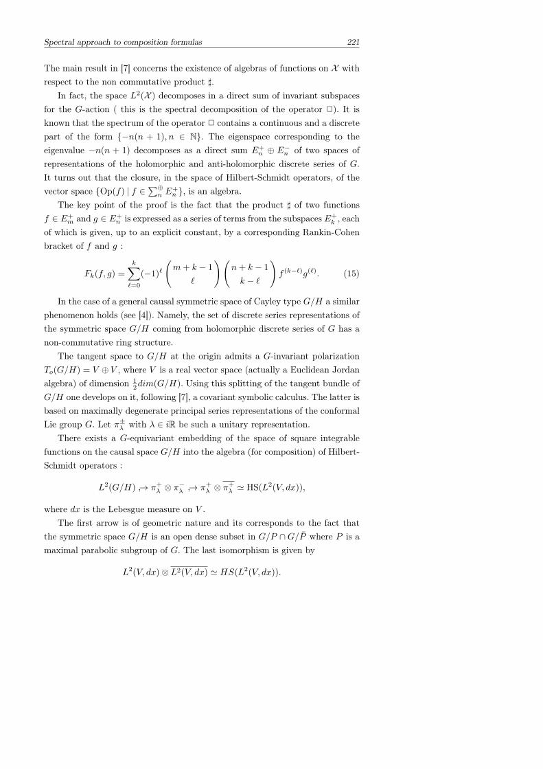
Spectral approach to composition formulas 221
The main result in [7] concerns the existence of algebras of functions on X withrespect to the non commutative product ].
In fact, the space L2(X ) decomposes in a direct sum of invariant subspacesfor the G-action ( this is the spectral decomposition of the operator 2). It isknown that the spectrum of the operator 2 contains a continuous and a discretepart of the form −n(n + 1), n ∈ N. The eigenspace corresponding to theeigenvalue −n(n + 1) decomposes as a direct sum E+
n ⊕ E−n of two spaces ofrepresentations of the holomorphic and anti-holomorphic discrete series of G.It turns out that the closure, in the space of Hilbert-Schmidt operators, of thevector space Op(f) | f ∈
∑⊕n E
+n , is an algebra.
The key point of the proof is the fact that the product ] of two functionsf ∈ E+
m and g ∈ E+n is expressed as a series of terms from the subspaces E+
k , eachof which is given, up to an explicit constant, by a corresponding Rankin-Cohenbracket of f and g :
Fk(f, g) =
k∑`=0
(−1)`
(m+ k − 1
`
)(n+ k − 1
k − `
)f (k−`)g(`). (15)
In the case of a general causal symmetric space of Cayley type G/H a similarphenomenon holds (see [4]). Namely, the set of discrete series representations ofthe symmetric space G/H coming from holomorphic discrete series of G has anon-commutative ring structure.
The tangent space to G/H at the origin admits a G-invariant polarizationTo(G/H) = V ⊕ V , where V is a real vector space (actually a Euclidean Jordanalgebra) of dimension 1
2dim(G/H). Using this splitting of the tangent bundle ofG/H one develops on it, following [7], a covariant symbolic calculus. The latter isbased on maximally degenerate principal series representations of the conformalLie group G. Let π±λ with λ ∈ iR be such a unitary representation.
There exists a G-equivariant embedding of the space of square integrablefunctions on the causal space G/H into the algebra (for composition) of Hilbert-Schmidt operators :
L2(G/H) → π+λ ⊗ π
−λ → π+
λ ⊗ π+λ ' HS(L2(V, dx)),
where dx is the Lebesgue measure on V .The first arrow is of geometric nature and its corresponds to the fact that
the symmetric space G/H is an open dense subset in G/P ∩G/P where P is amaximal parabolic subgroup of G. The last isomorphism is given by
L2(V, dx)⊗ L2(V, dx) ' HS(L2(V, dx)).
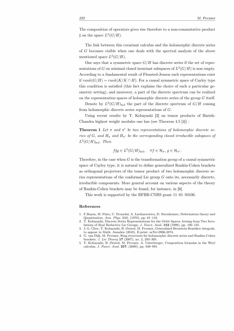
222 M. Pevzner
The composition of operators gives rise therefore to a non-commutative product] on the space L2(G/H).
The link between this covariant calculus and the holomorphic discrete seriesof G becomes visible when one deals with the spectral analysis of the abovementioned space L2(G/H).
One says that a symmetric space G/H has discrete series if the set of repre-sentations of G on minimal closed invariant subspaces of L2(G/H) is non empty.According to a fundamental result of Flensted-Jensen such representations existif rank(G/H) = rank(K/K ∩H). For a causal symmetric space of Cayley typethis condition is satisfied (this fact explains the choice of such a particular ge-ometric setting), and moreover, a part of the discrete spectrum can be realizedon the representation spaces of holomorphic discrete series of the group G itself.
Denote by L2(G/H)hol the part of the discrete spectrum of G/H comingfrom holomorphic discrete series representations of G.
Using recent results by T. Kobayashi [2] on tensor products of Harish-Chandra highest weight modules one has (see Theorem 4.5 [4]) :
Theorem 1 Let π and π′ be two representations of holomorphic discrete se-ries of G, and Hπ and Hπ′ be the corresponding closed irreducible subspaces ofL2(G/H)hol. Then
f]g ∈ L2(G/H)hol, ∀f ∈ Hπ, g ∈ Hπ′ .
Therefore, in the case when G is the transformation group of a causal symmetricspace of Cayley type, it is natural to define generalized Rankin-Cohen bracketsas orthogonal projectors of the tensor product of two holomorphic discrete se-ries representations of the conformal Lie group G onto its, necessarily discrete,irreducible components. More general account on various aspects of the theoryof Rankin-Cohen brackets may be found, for instance, in [6].
This work is supported by the RFBR-CNRS grant 11–01–93106.
References
1. F.Bayen, M. Flato, C. Fronsdal, A. Lischnerowicz, D. Sternheimer, Deformation theory andQuantization. Ann. Phys. 111, (1978), pp. 61–110.
2. T. Kobayashi, Discrete Series Representations for the Orbit Spaces Arising from Two Invo-lutions of Real Reductive Lie Groups, J. Funct. Anal. 152 (1998), pp. 100–135.
3. J.-L. Clerc, T. Kobayashi, B. Ørsted, M. Pevzner, Generalized Bernstein-Reznikov integrals,to appear in Math. Annalen (2010). E-print: arXiv:0906.2874.
4. G. van Dijk, M. Pevzner, Ring structures for holomorphic discrete series and Rankin-Cohenbrackets. J. Lie Theory 17 (2007), no. 2, 283–305.
5. T. Kobayashi, B. Ørsted, M. Pevzner, A. Unterberger, Composition formulas in the Weylcalculus, J. Funct. Anal. 257, (2009), pp. 948–991.

6. M. Pevzner, Covariant quantization: spectral analysis versus deformation theory. Jpn. J.Math. 3 (2008), no. 2, 247–290.
7. A. Unterberger, J. Unterberger, Algebras of symbols and modular forms. J. Anal. Math.68, (1996), pp. 121–143.
8. A. Unterberger, Automorphic pseudodifferential analysis and higher level Weyl calculi.Progress in Mathematics, 209. Birkhauser Verlag, Basel, 2003.
Michael PevznerUniversite de Reims, Reims, FranceE-mail: [email protected]
Tropical and Idempotent Mathematics. Moscow, Russia, August 26–31, 2012
Tropicalization of systems biology models
Ovidiu RadulescuDima GrigorievVincent NoelSergei Vakulenko
Abstract Systems biology use networks of biochemical reactions as models forcellular process. The dynamics of reaction networks with many well separatedtime scales, is well captured by asymptotic models obtained by tropicalizationof the smooth dynamics, via the Litvinov-Maslov correspondence principle. Thetropicalized models can be used to check the global stability and to identifysensitive parameters and rapid variables of the original models.
1. Introduction
In the last decade, systems biology became the playground of several mathemat-ical fields of study, among which algebraic geometry is one of the most impor-tant. Cellular biochemistry can be suitably modelled by networks of reactionswith rational and polynomial rate functions. The dynamics of these networkscan be described by rational or polynomial ODEs, for which some results existconcerning the type and the complexity of the solutions.
Most of the previous algebraic work on reaction networks was dedicated tothe study of steady states [CTF06,Sou03,Son05,RLS+06,RSP+11]. This issue isimportant, because networks with multiple stable steady states control biologicalcell fate decisions in development and differentiation [T+98,Del49].
However, biological cell physiology relies preeminently upon network dynam-ics. To interpret stimuli, adapt to environmental changes, make decisions, the
Tropicalization of systems biology models 225
cells lean on the rich dynamical possibilities of regulatory networks. We saythat regulatory networks are flexible, because they can support, in principle,any type of attractors and spatial-temporal patterns [VR12]. Networks are alsorobust, because these patterns resist to perturbations and are maintained forwide ranges of parameter values [GR07,RGZL08]. To achieve robust and flexi-ble functioning, biological networks employ hierarchies of biochemical processeswith well separated time scales.
Tropical geometry is well adapted for studying robust and flexible, multi-scale, biochemical networks. In [NGVR12] we used the Litvinov-Maslov corre-spondence principle to tropicalize rational or polynomial ODE models of bio-chemical networks. The tropicalization make it possible to develop geometricalmethods for critical parameter identification and for studying the qualitativedependence of the model dynamics on these parameters. These methods arebased on arrangements of tropical manifolds, reminding combinatorial methodssuch as polyhedral complexes used in tropical convexity [AD09], or geometricanalysis of S-systems proposed by [SCF+09] in relation to biochemical networksteady states design. Another application of the tropicalization is the detectionof quasi-steady and quasi-equilibrium conditions, that are very useful for modelreduction.
2. Settings
In chemical kinetics, the reagent concentrations satisfy ordinary differential equa-tions:
dxidt
= Fi(x), 1 ≤ i ≤ n. (1)
Rather generally, the rates are rational functions of the concentrations and read
Fi(x) = Pi(x)/Qi(x), (2)
where Pi(x) =∑α∈Ai
ai,αxα, Qi(x) =
∑β∈Bi
bi,βxβ , are multivariate polyno-
mials. Here xα = xα11 xα2
2 . . . xαnn , xβ = xβ1
1 xβ2
2 . . . xβnn , ai,α, bi,β , are nonzero real
numbers, and Ai, Bi are finite subsets of Nn.Special case are represented by
Fi(x) = P+i (x)− P−i (x), (3)
where P+i (x), P−i (x) are Laurent polynomials with positive coefficients,
P±i (x) =∑α∈A±i
a±i,αxα, a±i,α > 0, A±i are finite subsets of Zn. Real powers
A±i ⊂ Rn are sometimes used for the so-called S-systems [SCF+09].
226 O. Radulescu, D. Grigoriev, V. Noel, S. Vakulenko
Litvinov and Maslov [LMS01, LM96] proposed a heuristic (correspondenceprinciple) allowing to transform mathematical objects (integrals, polynomials)into their quantified (tropical) versions. According to this heuristic, to a Lau-rent polynomial with positive real coefficients
∑α∈A aαx
α, where A ⊂ Zn
is the support of the polynomial, one associates the max-plus polynomialmaxα∈Alog(aα)+ < log(x), α >. This heuristic can be used to associate apiecewise-smooth hybrid model to the system of rational ODEs (1), in two dif-ferent ways.
The first method was proposed in [NGVR12] and can be applied to anyrational ODE system defined by (1),(2):
Definition 1 We call complete tropicalization of the smooth ODE system (3)the following piecewise-smooth system:
dxidt
= DomPi(x)/DomQi(x), (4)
where Domai,αxαα∈Ai= sign(ai,αmax
)exp[maxα∈Ailog(|ai,α|)+ < u, α >].
u = (logx1, . . . , logxn), and ai,αmax, αmax ∈ Ai denote the coefficient of the
monomial for which the maximum is attained.
The second method,proposed in [SCF+09], applies to the systems (1),(3).
Definition 2 We call two terms tropicalization of the smooth ODE system (1)the following piecewise-smooth system:
dxidt
= DomP+i (x)−DomP−i (x), (5)
The two-terms tropicalization was used in [SCF+09] to analyse the depen-dence of steady states on the model parameters. The complete tropicalization wasused for the study of the model dynamics and for the model reduction [NGVR12].
For both tropicalization methods, for each occurrence of the Dom operator,one can introduce a tropical manifold, defined as the subset of Rn where themaximum in Dom is attained at least twice. For instance, for n = 2, such tropicalmanifold is made of points, segments connecting these points, and half-lines. Thetropical manifolds in such an arrangement decompose the space into sectors,inside which one monomial dominates all the others in the definition of thereagent rates. The combinatorial study of the arrangement give hints on thepossible steady states and attractors, as well as on their bifurcations.
Tropicalization of systems biology models 227
3. Justification of the tropicalization and some estimates
In the general case, the tropicalization heuristic is difficult to justify by rigorousestimates, however, this is possible in some cases. We state here some results inthis direction. Let us consider the class of polynomial systems, corresponding tomass action law chemical kinetics:
dxidt
= Fi(x, ε) =
M∑j=1
Fij(x, ε), Fij = Pij(ε)xαij (6)
where αij are multi-indices, and ε is a small parameter. So, the right hand sideof (6) is a sum of monomials. We suppose that coefficients Pij have differentorders in ε:
Pij(ε) = εbij Pij , (7)
where bij 6= bi′j′ for (i, j) 6= (i′, j′).We also suppose that the coneR> = x : xi ≥ 0 is invariant under dynamics
(6) and initial data are positive:
xi(0) > δ > 0.
The terms (7) can have different signs, the ones with Pij > 0 are productionterms, and those with Pij < 0 are degradation terms.
From the biochemical point of view, the choice (7) is justified by the multi-scaleness of the biochemical processes. Furthermore, we are interested in bio-chemical circuits that can function “stably” even in extremal conditions. Moreprecisely, we use the permanence concept, borrowed from the theory of speciescoexistence (the Lotka -Volterra model, see for instance [Tak96]).
Definition 3 The system (6) is permanent, if there are two constants C− > 0
and C+ > 0 such that
C− < xi(t) < C+, for all t > T0(x(0)) and for every i. (8)
We assume that C± and T0 are uniform in ε as ε→ 0.
This means that concentrations of all the reagents cannot vanish or becometoo big, even in extremal conditions. Biological oscillators, such as the circadianclock and the cell cycle, satisfy this condition. We can also consider systems (6)that become permanent after rescaling of the concentrations, xi = xiε
ai , such assystems with quasi-stationary, low concentration, reagents.
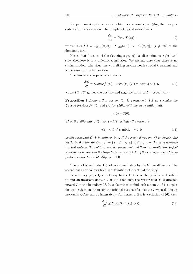
228 O. Radulescu, D. Grigoriev, V. Noel, S. Vakulenko
For permanent systems, we can obtain some results justifying the two pro-cedures of tropicalization. The complete tropicalization reads
dxidt
= Dom(Fi(x)), (9)
where Dom(Fi) = Fik(i)(x, ε), |Fik(i)(x, ε)| > |Fij(x, ε)|, j 6= k(i) is thedominant term.
Notice that, because of the changing sign, (9) has discontinuous right handside, therefore it is a differential inclusion. We assume here that there is nosliding motion. The situation with sliding motion needs special treatment andis discussed in the last section.
The two terms tropicalization reads
dxidt
= Dom(F+i (x))−Dom(F−i (x)) = Dom2(Fi(x)), (10)
where F+i , F−i gather the positive and negative terms of Fi, respectively.
Proposition 1 Assume that system (6) is permanent. Let us consider theCauchy problem for (6) and (9) (or (10)), with the same initial data:
x(0) = x(0).
Then the difference y(t) = x(t)− x(t) satisfies the estimate
|y(t)| < C1εγ exp(bt), γ > 0, (11)
positive constant C1, b is uniform in ε. If the original system (6) is structurallystable in the domain ΩC−,C+ = x : C− < |x| < C+, then the correspondingtropical systems (9) and (10) are also permanent and there is a orbital topologicalequivalency hε between the trajectories x(t) and x(t) of the corresponding Cauchyproblems close to the identity as ε→ 0.
The proof of estimate (11) follows immediately by the Gronwall lemma. Thesecond assertion follows from the definition of structural stability.
Permanency property is not easy to check. One of the possible methods isto find an invariant domain I in Rn such that the vector field F is directedinward I at the boundary ∂I. It is clear that to find such a domain I is simplerfor tropicalizations than for the original system (for instance, when dominantmonomial ODEs can be integrated). Furthermore, if x is a solution of (6), then
dxidt≤ K(ε)|Dom(Fi(x, ε))|, (12)
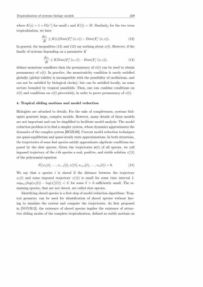
Tropicalization of systems biology models 229
where K(ε) = 1 +O(εγ) for small ε and K(1) = M . Similarly, for the two termtropicalization, we have
dxidt≤ K(ε)Dom(F+
i (x, ε))−Dom(F−i (x, ε)). (13)
In general, the inequalities (13) and (12) say nothing about x(t). However, if thefamily of systems depending on a parameter K
dxidt≤ KDom(F+
i (x, ε))−Dom(F−i (x, ε)). (14)
defines monotone semiflows then the permanency of x(t) can be used to obtainpermanency of x(t). In practice, the monotonicity condition is rarely satisfiedglobally (global validity is incompatible with the possibility of oscillations, andcan not be satisfied by biological clocks), but can be satisfied locally, on somesectors bounded by tropical manifolds. Then, one can combine conditions onx(t) and conditions on x(t) piecewisely, in order to prove permanency of x(t).
4. Tropical sliding motions and model reduction
Biologists are attached to details. For the sake of completeness, systems biol-ogists generate large, complex models. However, many details of these modelsare not important and can be simplified to facilitate model analysis. The modelreduction problem is to find a simpler system, whose dynamics approximates thedynamics of the complex system [RGZL08]. Current model reduction techniquesuse quasi-equilibrium and quasi-steady state approximations. In both situations,the trajectories of some fast species satisfy approximate algebraic conditions im-posed by the slow species. Given the trajectories x(t) of all species, we callimposed trajectory of the i-th species a real, positive, and stable solution x∗i (t)of the polynomial equation
Pi(x1(t), . . . , xi−1(t), x∗i (t), xi+1(t), . . . , xn(t)) = 0, (15)
We say that a species i is slaved if the distance between the trajectoryxi(t) and some imposed trajectory x∗i (t) is small for some time interval I,supt∈I |log(xi(t)) − log(x∗i (t))| < δ, for some δ > 0 sufficiently small. The re-maining species, that are not slaved, are called slow species.
Identifying slaved species is a first step of model reduction algorithms. Trop-ical geometry can be used for identification of slaved species without hav-ing to simulate the system and compute the trajectories. As first proposedin [NGVR12], the existence of slaved species implies the existence of attrac-tive sliding modes of the complete tropicalization, defined as stable motions on
230 O. Radulescu, D. Grigoriev, V. Noel, S. Vakulenko
the tropical manifold. Attractive sliding modes are possible in the theory ofpiecewise-smooth systems [FA88] provided that the following condition is satis-fied, for x on the tropical manifold:
< n+(x), f+(x) >< 0, < n−(x), f−(x) >< 0 (16)
where f+, f− are the dominant vector fields on the two sides of a tropical hyper-surface and n+ = −n− are the normals to the interior faces.
References
[AD09] F. Ardila and M. Develin. Tropical hyperplane arrangements and oriented matroids.Mathematische Zeitschrift, 262(4):795–816, 2009.
[CTF06] G. Craciun, Y. Tang, and M. Feinberg. Understanding bistability in complexenzyme-driven reaction networks. Proceedings of the National Academy of Sci-ences, 103(23):8697–8702, 2006.
[Del49] M. Delbruck. Discussion: Unitees biologiques douees de continuite genetique. InActes du colloque international du CNRS, pages 33–3, Paris, 1949. Editions duCNRS.
[FA88] A.F. Filippov and FM Arscott. Differential equations with discontinuous righthandsides, volume 18. Springer, 1988.
[GR07] A. N. Gorban and O. Radulescu. Dynamical robustness of biological networks withhierarchical distribution of time scales. IET Systems Biology, 1:238–246, 2007.
[LM96] G.L. Litvinov and V.P. Maslov. Idempotent mathematics: a correspondence princi-ple and its applications to computing. Russian Mathematical Surveys, 51(6):1210–1211, 1996.
[LMS01] G.L. Litvinov, V.P. Maslov, and G.B. Shpiz. Idempotent functional analysis: analgebraic approach. Mathematical Notes, 69(5):696–729, 2001.
[NGVR12] V. Noel, D. Grigoriev, S. Vakulenko, and O. Radulescu. Tropical geometries anddynamics of biochemical networks. Application to hybrid cell cycle models. Elec-tronic Notes in Theoretical Computer Science, 284:75–91, 2012.
[RGZL08] O. Radulescu, A. N. Gorban, A. Zinovyev, and A. Lilienbaum. Robust simplifica-tions of multiscale biochemical networks. BMC Systems Biology, 2(1):86, 2008.
[RLS+06] O. Radulescu, S. Lagarrigue, A. Siegel, P. Veber, and M. Le Borgne. Topology andstatic response of interaction networks in molecular biology. Journal of The RoyalSociety Interface, 3(6):185–196, 2006.
[RSP+11] O. Radulescu, A. Siegel, E. Pecou, C. Chatelain, and S. Lagarrigue. Geneticallyregulated metabolic networks: Gale-Nikaido modules and differential inequalities.Transactions on computational systems biology XIII, pages 110–130, 2011.
[SCF+09] M.A. Savageau, P.M.B.M. Coelho, R.A. Fasani, D.A. Tolla, and A. Salvador. Phe-notypes and tolerances in the design space of biochemical systems. Proceedings ofthe National Academy of Sciences, 106(16):6435, 2009.
[Son05] E.D. Sontag. Molecular systems biology and control. European Journal of Control,11:396–435, 2005.
[Sou03] C. Soule. Graphic requirements for multistationarity. Complexus, 1(123-133), 2003.[T+98] R. Thomas et al. Laws for the dynamics of regulatory networks. International
Journal of Developmental Biology, 42:479–485, 1998.[Tak96] Y. Takeuchi. Global dynamical properties of Lotka-Volterra systems. World Scien-
tific, Singapore, 1996.[VR12] S. Vakulenko and O. Radulescu. Flexible and robust patterning by centralized gene
networks. Fundamenta Informaticae, 118:345–369, 2012.
Ovidiu RadulescuDIMNP UMR CNRS 5235, University of Montpellier 2, Montpellier, France

E-mail: [email protected]
Dima GrigorievCNRS, Mathematiques, Universite de Lille, 59655, Villeneuve d’Ascq, France
Vincent NoelIRMAR UMR 6625, University of Rennes 1, Rennes, France
Sergei VakulenkoSaint Petersburg State University of Technology and Design, St.Petersburg, Rus-sia
Tropical and Idempotent Mathematics. Moscow, Russia, August 26–31, 2012
Layered tropical algebras, applied to tropical alge-braic geometry
Louis Rowen
Tropical mathematics is defined over an ordered cancellative monoid M,usually taken to be (R,+) or (Q,+). An algebraic description of the max-plusalgebra: We say that a semiring is bipotent if a+ b ∈ a, b for all a, b. There isa 1:1 correspondence between ordered monoids (M, <) and bipotent semiringsA, where A =M as a monoid. Namely, multiplication in A is the given monoidoperation, and addition in A is defined by a + b = maxa, b. Every bipotentsemiring is idempotent, since a+ a ∈ a, a = a.
Customarily, tropical curves have been defined either combinatorially interms of two monomials having equal (leading) values, or synthetically as do-mains of non-differentiability of polynomials over the max-plus algebra satisfyingthe “balancing condition.” Also tropical mathematics has been viewed in termsof valuation theory applied to curves over Puiseux series.
Although there is a rich theory arising from this viewpoint, cf. [7], idempotentsemirings possess a restricted algebraic structure theory, and also do not reflectcertain valuation-theoretic properties, thereby forcing researchers to rely oftenon combinatoric techniques.
Example 1 Consider the polynomial f(a) = λ3 + aλ2 + a3, viewed tropically(over a bipotent algebra A). Note that f(b) = b3 when b > a and f(b) = a3
when b < a. Likewise, f(a) = a3 has three equal values for the monomials, soa is a tropical root, and there are no others, although one could not detect thisdirectly from the value f(a) = a3.
The object of this talk is to describe an alternative structure studied over thepast few years by Izhakian, Knebusch, and Rowen [4] (with a more categorical
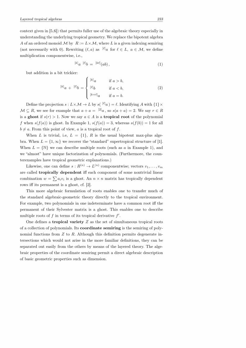
Layered tropical algebras 233
context given in [5,6]) that permits fuller use of the algebraic theory especially inunderstanding the underlying tropical geometry. We replace the bipotent algebraA of an ordered monoidM by R := L×M, where L is a given indexing semiring(not necessarily with 0). Rewriting (`, a) as [`]a for ` ∈ L, a ∈ M, we definemultiplication componentwise, i.e.,
[k]a [`]b = [k`](ab) , (1)
but addition is a bit trickier:
[k]a + [`]b =
[k]a if a > b,
[`]b if a < b,
[k+`]a if a = b.
(2)
Define the projection s : L×M→ L by s( [`]a ) = `. Identifying A with 1×M ⊆ R, we see for example that a + a = [2]a , so s(a + a) = 2. We say r ∈ Ris a ghost if s(r) > 1. Now we say a ∈ A is a tropical root of the polynomialf when s(f(a)) is ghost. In Example 1, s(f(a)) = 3, whereas s(f(b)) = 1 for allb 6= a. From this point of view, a is a tropical root of f .
When L is trivial, i.e, L = 1, R is the usual bipotent max-plus alge-bra. When L = 1,∞ we recover the “standard” supertropical structure of [1].When L = N we can describe multiple roots (such as a in Example 1), andwe “almost” have unique factorization of polynomials. (Furthermore, the coun-terexamples have tropical geometric explanations.)
Likewise, one can define s : R(n) → L(n) componentwise; vectors v1, . . . , vmare called tropically dependent iff each component of some nontrivial linearcombination w =
∑aivi is a ghost. An n × n matrix has tropically dependent
rows iff its permanent is a ghost, cf. [2].This more algebraic formulation of roots enables one to transfer much of
the standard algebraic-geometric theory directly to the tropical environment.For example, two polynomials in one indeterminate have a common root iff thepermanent of their Sylvester matrix is a ghost. This enables one to describemultiple roots of f in terms of its tropical derivative f ′.
One defines a tropical variety Z as the set of simultaneous tropical rootsof a collection of polynomials. Its coordinate semiring is the semiring of poly-nomial functions from Z to R. Although this definition permits degenerate in-tersections which would not arise in the more familiar definitions, they can beseparated out easily from the others by means of the layered theory. The alge-braic properties of the coordinate semiring permit a direct algebraic descriptionof basic geometric properties such as dimension.
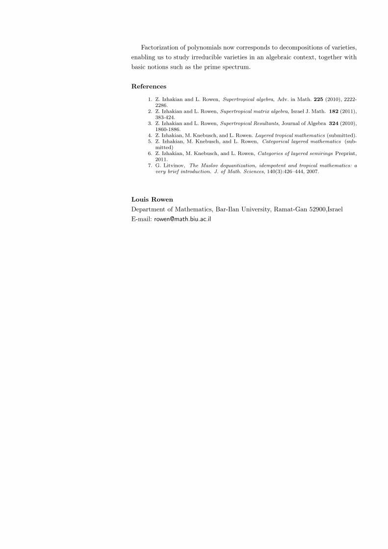
Factorization of polynomials now corresponds to decompositions of varieties,enabling us to study irreducible varieties in an algebraic context, together withbasic notions such as the prime spectrum.
References
1. Z. Izhakian and L. Rowen, Supertropical algebra, Adv. in Math. 225 (2010), 2222-2286.
2. Z. Izhakian and L. Rowen, Supertropical matrix algebra, Israel J. Math. 182 (2011),383-424.
3. Z. Izhakian and L. Rowen, Supertropical Resultants, Journal of Algebra 324 (2010),1860-1886.
4. Z. Izhakian, M. Knebusch, and L. Rowen. Layered tropical mathematics (submitted).5. Z. Izhakian, M. Knebusch, and L. Rowen, Categorical layered mathematics (sub-
mitted)6. Z. Izhakian, M. Knebusch, and L. Rowen, Categories of layered semirings Preprint,
2011.7. G. Litvinov, The Maslov dequantization, idempotent and tropical mathematics: a
very brief introduction. J. of Math. Sciences, 140(3):426–444, 2007.
Louis RowenDepartment of Mathematics, Bar-Ilan University, Ramat-Gan 52900,IsraelE-mail: [email protected]
Tropical and Idempotent Mathematics. Moscow, Russia, August 26–31, 2012
On idempotents in compactleft topological universal algebras
Denis I. Saveliev
Abstract A standard fact important for applications is that any compact lefttopological semigroup has an idempotent. We extend this to certain compactleft topological universal algebras.
A well-known fact is that any compact left topological semigroup has anidempotent, i.e. an element forming a subsemigroup. This firstly was establishedfor compact topological semigroups independently by Numakura [1] and Wal-lace [2,3], and in the final form (perhaps) by Ellis in [4]. This fact, despite of itseasy proof, is fundamental for Ramsey-theoretic applications in number theory,algebra, topological dynamics, and ergodic theory. Hindman’s Finite ProductsTheorem, van der Waerden’s and Szemeredy’s Arithmetic Progressions The-orems, and Furstenberg’s Multiple Recurrence Theorem can be mentioned aswidely known examples. Most of such applications have no (known) alternativeproofs. The crucial fact for all them is the existence of idempotent ultrafiltersover semigroups.
Let us shortly recall what are idempotent ultrafilters. The set ββX of ultra-filters over a set X with a natural topology generated by basic (cl)open setsu ∈ ββX : S ∈ u, S ⊆ X, forms the largest (Stone–Cech or Wallman) compact-ification of the discrete space X. If · is a binary operation on X, it extends toa binary operation on ββX by letting for all u, v ∈ ββX
uv =S ⊆ X : a ∈ X : b ∈ X : ab ∈ S ∈ u ∈ v
.
236 D. Saveliev
The extended operation is continuous in any first argument, i.e. the groupoid(ββX, · ) is left topological, and in any second argument whenever it is in X. Notmany algebraic properties are stable under this extension, but associativity is.Hence any semigroupX extends to a compact left topological semigroup ββX, andtherefore, there exists an ultrafilter u ∈ ββX that is an idempotent of the extendedoperation. The book [5] is a comprehensive treatise on ultrafilter extensions ofsemigroups and various applications, with some historical remarks.
The ultrafilter extension actually is a general construction. As we shownin [6], arbitrary first-order model on X, i.e. a set X with operations and rela-tions on it, canonically extends to the model on ββX such that its model-theoreticproperties are, in a sense, completely analogous to the topological propertiesof ββX. Certainly, not all extended models contain idempotents, associativity isessential in Ellis’ result. In this note, we replace it by other, much wider alge-braic conditions thus showing that compact left topological universal algebrassatisfying these conditions have single-point subalgebras. We also mention appli-cations using idempotent ultrafilters over such algebras. For simplicity, we shallconsider only algebras with one or two binary operations; this suffices however todemonstrate related ideas. General results in this direction can be found in [7].
Fix some terminology. An algebra is a universal algebra, i.e. a set with arbi-trary operations of any arities on it. A groupoid is an algebra with one binaryoperation. As a rule, we call the operation a multiplication and write rather xythan x · y. If F is an n-ary operation on X, its idempotent is an a ∈ X such thatF (a, . . . , a) = a. An idempotent of an algebra is a common idempotent of all itsoperations, i.e. an element forming a subalgebra.
In the sequel, all topological spaces are assumed to be Hausdorff. An algebraendowed with a topology is left topological iff for any its operation F , the unarymap
x 7→ F (a1, . . . , an, x)
is continuous, for any fixed a1, . . . , an ∈ X. Right topological algebras are defineddually. An algebra is semitopological iff all unary maps obtained from any of itsoperation by fixing all but one arguments are continuous, and topological iff allits operations are continuous. In particular, a groupoid is semitopological iff itis left and right topological simultaneously, and topological if its multiplicationis continuous. This hierarchy does not degenerate, even for compact semigroups(see e.g. [5]).
An algebra is minimal iff it includes no proper subalgebras, and minimalcompact iff it carries a compact topology and includes no proper compact subal-
On idempotents in compact algebras 237
gebra. Clearly, an algebra may include no minimal subalgebra. Contrary to this,any compact algebra does include a minimal compact subalgebra (apply Zorn’sLemma to the family of compact subalgebras ordered by inclusion). As we shallsee, certain algebraic properties restrict possible size of minimal and minimalcompact algebras.
An occurrence of a variable x into a term t(x, . . .) is right-most iff whenever
t1(x, . . .) · t2(x, . . .)
is a subterm of t, then x occurs into t2(x, . . .) but not t1(x, . . .). E.g. all theoccurrences of the variable x into the terms x, vx, v(vx), (v1v2)(v3x) are right-most, while all its occurrences into the terms v, xv, x(vx), (v1x)(v2x) are not.A left-most occurrence is defined dually. Clearly, if the occurrence of x into t isright-most (or left-most), then x occurs there exactly once.
It easy to see that if X is a left topological algebra and t(v1, . . . , vn, x) a termwith the right-most occurrence of the last argument, then the map
x 7→ t(a1, . . . , an, x)
is continuous, for any fixed a1, . . . , an ∈ X.The following theorem generalizes Ellis’ result to certain groupoids.
Theorem 1 Let X be a compact left topological groupoid, r(v1), s(v1, v2), andt(v1, v2, v3) some terms, and let s(v1, v2) have the right-most occurrence of thelast argument. If X satisfies
s(x, y) · s(x, z) = s(x, t(x, y, z)) and
s(x, y) = s(x, z) = r(x) → s(x, yz) = r(x),
then it has an idempotent.
Proof (Scetch of proof) The conditions of Theorem 1 are universal formulas, soany subgroupoid of X should satisfy them. By Zorn’s Lemma, isolate a minimalcompact subgroupoid A and show that A consists of a single point. Pick anya ∈ A. The map x 7→ s(a, x) is continuous since the occurrence of x in s(v, x)is right-most. Hence the first condition implies that s(a,A) = s(a, b) : b ∈A is a compact subgroupoid of A, whence s(a,A) = A, and so B = b ∈A : s(a, b) = r(a) is nonempty. Now the second condition implies that B isa compact subgroupoid of A, whence B = A, and then aa = a by the firstcondition.
238 D. Saveliev
Although the conditions of Theorem 1 look technical, they follow from variouseasy particular identities. Thus any compact left topological groupoids satisfyingsuch identities does have an idempotent. Let us give some examples.
First af all, the associativity law implies the conditions, with r(v) = v,s(v1, v2) = v1v2, t(v1, v2, v3) = v2v1v3. Thus Ellis’ result follows from Theo-rem 1.
Next, let us call the following identity
x(yz) = (xz)y
left skew associativity and groupoids satisfying it left skew semigroups. The iden-tity clearly follows from conjunction of associativity and commutativity butimplies neither of them. Left skew associativity also implies the conditions ofTheorem 1, with r(v) = v, s(v1, v2) = v1v2, t(v1, v2, v3) = (v1v3)v2. Thus we see:Any compact left topological left skew semigroup has an idempotent.
There are many identities strictly weaker than associativity that imply theconditions of Theorem 1. E.g., so is the identity (of Bol–Moufang type)
(xx)(yz) = ((xx)y)z.
Here r(v) = vv, s(v1, v2) = (v1v1)v2, t(v1, v2, v3) = v2((v1v1)v3). Examples ofsuch kind can be easily multiplied.
Using of the conditions of Theorem 1 is essential; in general, neither min-imal compact left topological groupoids, neither minimal groupoids, when thelatter exist, need consist of a single point. E.g. there exist countable minimalquasigroups (see [7]). To mention a topological counterpart, consider the identity
x(yz) = (xy)(xz),
called left distributivy . Thus a groupoid (X, · ) satisfies it iff the map x 7→ ax
is its endomorphism, for any fixed a ∈ X. Right distributivity is defined dually,and distributivity is the conjunction of left and right versions.
Such groupoids arise in knot theory, where they usually are idempotents,and also in set theory, where, as Laver shown, nontrivial elementary embeddingsof Vδ into itself with their application operation f · g =
⋃α<δ f(g Vα) form
a free left distributive groupoid without minimal subgroupoids. The existenceof such embeddings is an extremely large cardinal axiom, and it is still a majoropen problem whether the axiom is necessary to prove a purely algebraic factabout certain finite left distributive groupoids, so-called Laver’s tables (see [8]and references there).
On idempotents in compact algebras 239
Jezek and Kepka shown that in distributive groupoids, all (wx)(yz), and soall terms with more than 2 occurrences, are idempotents (see [9]). The one-sided case differs; in [10] we shown: All minimal left distributive groupoids arefinite, and for any finite n there exists exactly one (up to isomorphism) suchgroupoid of cardinality n. There exists a minimal compact topological left dis-tributive groupoid of cardinality 22
ℵ0. (The proof of the latter fact uses algebraof ultrafilters.)
Let us discuss an application of Theorem 1. As mentioned, any groupoiduniquely extends to the compact left topological algebra of ultrafilters over it;moreover, associativity is stable under this extension, so any semigroup extendsto the semigroup of ultrafilters over it. One can ask about more stable identities.Elsewhere we prove: Let an identity s1 = s2 be equivalent to some identity t1 = t2
such that the common variables of t1 and t2 appear in these terms in the sameordering, and any common variable occurs in each of the terms only once. Thenthe identity s1 = s2 is stable under ββ . In particular, identities that follow fromassociativity are stable under ββ whenever one of its terms is repeatless, i.e. eachvariable occurs in it at most once. (On the other hand, it can be shown thate.g. neither commutativity, nor idempotency is stable.)
An interesting case is when some identities are stable under ββ and in the sametime imply the conditions of Theorem 1. If a groupoid satisfies such identities,one can apply Theorem 1 to the groupoid of ultrafilters over it, thus obtainingan idempotent ultrafilter. The identity
(wx)(yz) = ((wx)y)z
is an example. It is stable under ββ (by the criterion above) and implies theweaker identity (xx)(yz) = ((xx)y)z, which in turn implies the conditions ofTheorem 1 (as noted above). Therefore, it provides an idempotent ultrafilter.(Note that we could not use the identity (xx)(yz) = ((xx)y)z, which is notrepeatless and actually is not stable under ββ .)
As mentioned, such ultrafilters allow to obtain significant combinatorial re-sults. E.g. the following version of Hindman’s Finite Products Theorem holds: Ifa groupoid X satisfies (wx)(yz) = ((wx)y)z, then any of its finite partitions hasa part containing a countable sequence a0, . . . , an, . . . together with finite products
an0(an1 . . . (ankank+1
) . . .)
for all n0 < n1 < . . . < nk < nk+1. Moreover, if X does not have idempotents oris right cancellative, one can find such a sequence consisting of pairwise distinctelements. For the proof and various refinements, see [11].
240 D. Saveliev
Theorem 1 can be generalized to the case of one operation of arbitrary arity,in the expected way. Let us now pass to algebras with many operations. Forsimplicity we consider only the case of two binary operations, denoted as additionand multiplication, although it is possible to establish a general result aboutarbitrary algebras, for which we refer to [7].
Theorem 2 Let (X,+, · ) be a compact left topological algebra such that anycompact subgroupoid of its additive groupoid (X,+) has an idempotent. Let q1(v),q2(v), r(v), s(v1, v2), t1(v1, v2, v3), t2(v1, v2, v3) be some terms, where q1(v),q2(v) are additive, and s(v1, v2) has the right-most occurence of the last ar-gument. If X satisfies
x+ x = x→r(x) + r(x) = r(x),
s(x, y) + s(x, z)=s(x, t1(x, y, z)),
s(x, y) · s(x, z)=s(x, t2(x, y, z)),
ands(x, y) = s(x, z) = r(x)→s(x, y + z) = q1(r(x)),
s(x, y) = s(x, z) = r(x)→s(x, yz) = q2(r(x)),
then it has an idempotent.
Proof (Scetch of proof) Let A be a minimal compact subalgebra of X, a ∈ A anadditive idempotent. The map x 7→ s(a, x) is continuous, hence the conditionsimply firstly that s(a,A) is a compact subalgebra of A, and secondly that B =
b ∈ A : s(a, b) = r(a) is a compact subalgebra of A, so B = A. Then aa = a
follows.
Theorem 2 extends Theorem 1 since any groupoid (X, · ) satisfying the condi-tions of Theorem 1, with some r, s, and t, can be turned into an algebra (X,+, · )satisfying the conditions of Theorem 2 by defining an extra operation + as theprojection onto the first argument: x+ y = x for all x ∈ X. In result, (X,+) isa left-zero semigroup, and one can put q1(v) = q2(v) = v, t1(v1, v2, v3) = v2, thesame r, s, and t as t2.
Let us consider some examples of identities implying the conditions of The-orem 2. The identity
x(y + z) = xy + xz
is left distributivy of · w.r.t. + . Thus an algebra (X,+, · ) satisfies it iff the mapx 7→ ax is an endomorphism of (X,+), for any fixed a ∈ X. If + and · coincide,this gives left distributive groupoids mentioned above. Right distributivity of ·
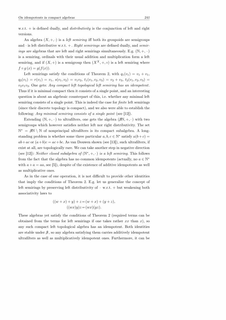
On idempotents in compact algebras 241
w.r.t. + is defined dually, and distributivity is the conjunction of left and rightversions.
An algebra (X,+, ·) is a left semiring iff both its groupoids are semigroupsand · is left distributive w.r.t. + . Right semirings are defined dually, and semir-ings are algebras that are left and right semirings simultaneously. E.g. (N,+, · )is a semiring, ordinals with their usual addition and multiplication form a leftsemiring, and if (X,+) is a semigroup then (XX ,+, ) is a left semiring wheref g (x) = g(f(x)).
Left semirings satisfy the conditions of Theorem 2, with q1(v1) = v1 + v1,q2(v1) = r(v1) = v1, s(v1, v2) = v1v2, t1(v1, v2, v3) = v2 + v3, t2(v1, v2, v3) =
v2v1v3. One gets: Any compact left topological left semiring has an idempotent .Thus if it is minimal compact then it consists of a single point, and an interestingquestion is about an algebraic counterpart of this, i.e. whether any minimal leftsemiring consists of a single point. This is indeed the case for finite left semirings(since their discrete topology is compact), and we also were able to establish thefollowing: Any minimal semiring consists of a single point (see [12]).
Extending (N,+, · ) to ultrafilters, one gets the algebra (ββN,+, · ) with twosemigroups which however satisfies neither left nor right distributivity. The setN∗ = ββN \ N of nonprincipal ultrafilters is its compact subalgebra. A long-standing problem is whether some three particular a, b, c ∈ N∗ satisfy a(b+ c) =
ab+ac or (a+b)c = ac+bc. As van Douwen shown (see [13]), such ultrafilters, ifexist at all, are topologically rare. We can take another step in negative direction(see [12]): Neither closed subalgebra of (N∗,+, · ) is a left semiring. This followsfrom the fact that the algebra has no common idempotents (actually, no a ∈ N∗
with a+a = aa, see [5]), despite of the existence of additive idempotents as wellas multiplicative ones.
As in the case of one operation, it is not difficult to provide other identitiesthat imply the conditions of Theorem 2. E.g. let us generalize the concept ofleft semirings by preserving left distributivity of · w.r.t. + but weakening bothassociativity laws to
((w + x) + y) + z=(w + x) + (y + z),
((wx)y)z=(wx)(yz).
These algebras yet satisfy the conditions of Theorem 2 (required terms can beobtained from the terms for left semirings if one takes rather xx than x), soany such compact left topological algebra has an idempotent. Both identitiesare stable under ββ , so any algebra satisfying them carries additively idempotentultrafilters as well as multiplicatively idempotent ones. Furthermore, it can be
242 D. Saveliev
shown that under left distribtivity of + w.r.t. · some multiplicatively idempotentultrafilters are in the closure of the set of additively idempotent ultrafilters.This fact leads to the following result (established by Hindman and Bergelsonfor the semiring of natural numbers, see [5]): If (X,+, · ) satisfies two identitiesabove and left distribtivity of + w.r.t. · , then any of its finite partitions hasa part containing countable sequences a0, . . . , an, . . . and b0, . . . , bn, . . . togetherwith finite sums
an0 + (an1 + . . .+ (ank+ ank+1
) . . .)
and productsbn0(bn1 . . . (bnk
bnk+1) . . .)
for all n0 < n1 < . . . < nk < nk+1. Moreover, if each of the operations does nothave idempotents or is right cancellative, one can find such sequences consistingof pairwise distinct elements. (See [11].)
Finally, let us consider algebras (X, , · ) satisfying the following identities:
(x y) z=x (y z),(x y)z=x(yz),x(y z)=xy xz,x y=xy x.
It follows that (X, · ) is a left distributive groupoid (and conversely, it can beshown that any left distributive groupoid extends to such an algebra). As Laverestablished, elementary embeddings with their application · and composition form algebras satisfying these identities (see [8]). Unlike the case of one leftdistributive operation, any such compact left topological algebra does have anidempotent: as (X, ) is a semigroup, it has an idempotent a, then it easily followsfrom the identities that aa is a common idempotent. We think that a study ofultrafilter extensions of these algebras could throw light upon the problem ofLaver’s tables.
References
1. K. Numakura. On bicompact semigroups. Math. J. Okayama Univ., 1 (1952), 99–108.2. A. Wallace. A note on mobs, I. An. Acad. Brasil. Cienc., 24 (1952), 329–334. A note on
mobs, II. An. Acad. Brasil. Cienc., 25 (1953), 335–336.3. A. Wallace. The structure of topological semigroups. Bull. Amer. Math. Soc., 61 (1955),
95–112.4. R. Ellis. Lectures on topological dynamics. Benjamin, N.Y., 1969.5. N. Hindman, D. Strauss. Algebra in the Stone–Cech compactification. W. de Gruyter,
Berlin–N.Y., 1998.6. D. I. Saveliev. Ultrafilter extensions of models. Lecture Notes in AICS, Springer, 6521
(2011), 162–177. An extended version in: S.-D. Friedman et al. (eds.). The Infinity Pro-ceedings. CRM Documents 11, Barcelona, 2012.
7. D. I. Saveliev. On the existence of idempotents in compact left topological universal al-gebras. Manuscript, 2008.
8. P. Dehornoy. Elementary embeddings and algebra. In: M. Foreman, A. Kanamori (eds.).Handbook of set theory. Springer, Berlin–N.Y., 2010.
9. D. Stanovsky. Distributive groupoids are symmetyric-by-medial: an elementary proof.Comment. Math. Univ. Carolinae, 49:4 (2008), 541–546.
10. D. I. Saveliev. Minimal and minimal compact left topological left distributive groupoids.www.karlin.mff.cuni.cz/∼ical/presentations/ saveliev.pdf.
11. D. I. Saveliev. On Hindman sets. Manuscript, 2008.12. D. I. Saveliev. Common idempotents in compact left topological left semirings.
arxiv:1002.1599.13. E. K. van Douwen. The Stone–Cech compactification of a discrete groupoid. Topol. Appl.,
39 (1991), 43–60.
Partly supported by RFBR grants 11-01-00958 and 11-01-93107, NSh grant5593-2012-1, and INFTY grant of ESF.
Denis I. SavelievM.V. Lomonosov Moscow State University, Moscow, Russia.E-mail: [email protected]
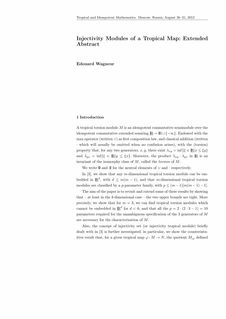
Tropical and Idempotent Mathematics. Moscow, Russia, August 26–31, 2012
Injectivity Modules of a Tropical Map: ExtendedAbstract
Edouard Wagneur
1 Introduction
A tropical torsion moduleM is an idempotent commutative semimodule over theidempotent commutative extended semiring IR = IR∪−∞. Endowed with themax operator (written ∨) as first composition law, and classical addition (written· which will usually be omitted when no confusion arises), with the (torsion)property that, for any two generators, x, y, there exist λxy = infξ ∈ IR|x ≤ ξyand λyx = infξ ∈ IR|y ≤ ξx. Moreover, the product λxy · λyx in IR is aninvariant of the isomorphy class of M , called the torsion of M .
We write 000 and 1l for the neutral elements of ∨ and · respectively.In [3], we show that any m-dimensional tropical torsion module can be em-
bedded in IRd, with d ≤ m(m − 1), and that m-dimensional tropical torsionmodules are classified by a p-parameter family, with p ≤ (m− 1)[m(m− 1)− 1].
The aim of the paper is to revisit and extend some of these results by showingthat – at least in the 3-dimensional case – the two upper bounds are tight. Moreprecisely, we show that for m = 3, we can find tropical torsion modules whichcannot be embedded in IRd for d < 6, and that all the p = 2 · (2 · 3 − 1) = 10
parameters required for the unambiguous specification of the 3 generators of Mare necessary for the characterization of M .
Also, the concept of injectivity set (or injectivity tropical module) brieflydealt with in [3] is further investigated. in particular, we show the counterintu-itive result that, for a given tropical map ϕ : M → N , the quotient M|ϕ defined
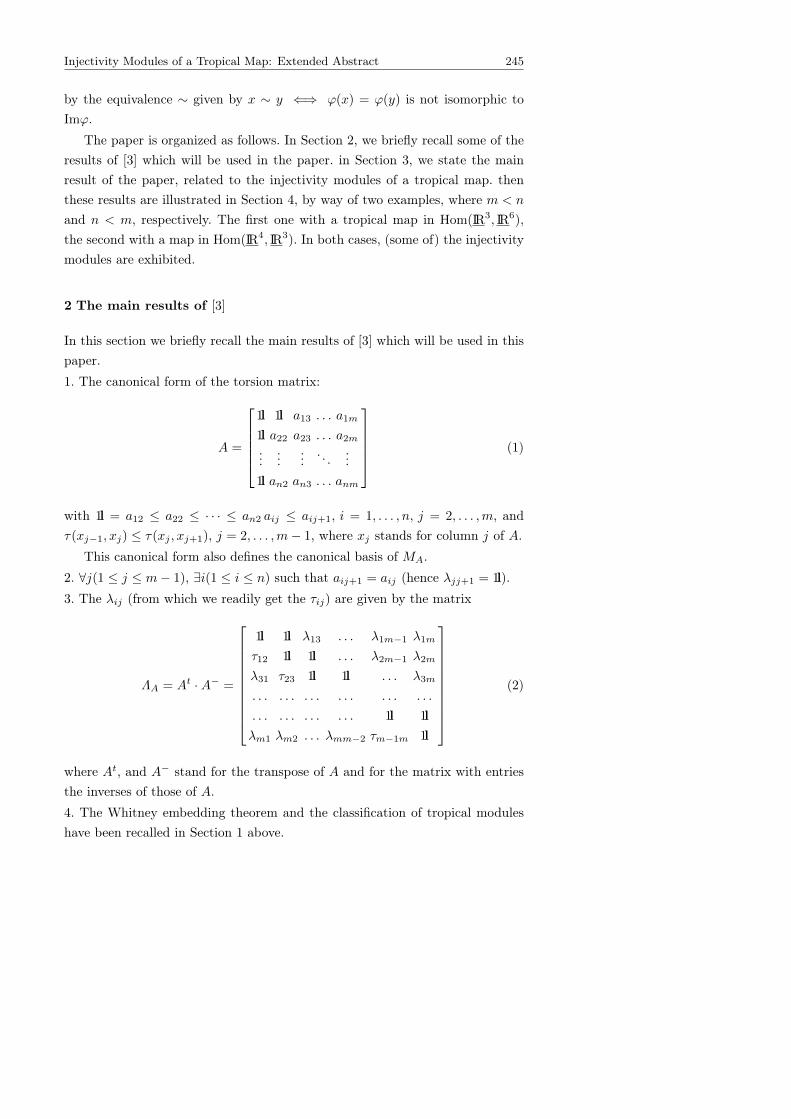
Injectivity Modules of a Tropical Map: Extended Abstract 245
by the equivalence ∼ given by x ∼ y ⇐⇒ ϕ(x) = ϕ(y) is not isomorphic toImϕ.
The paper is organized as follows. In Section 2, we briefly recall some of theresults of [3] which will be used in the paper. in Section 3, we state the mainresult of the paper, related to the injectivity modules of a tropical map. thenthese results are illustrated in Section 4, by way of two examples, where m < n
and n < m, respectively. The first one with a tropical map in Hom(IR3, IR6),the second with a map in Hom(IR4, IR3). In both cases, (some of) the injectivitymodules are exhibited.
2 The main results of [3]
In this section we briefly recall the main results of [3] which will be used in thispaper.
1. The canonical form of the torsion matrix:
A =
1l 1l a13 . . . a1m
1l a22 a23 . . . a2m...
......
. . ....
1l an2 an3 . . . anm
(1)
with 1l = a12 ≤ a22 ≤ · · · ≤ an2 aij ≤ aij+1, i = 1, . . . , n, j = 2, . . . ,m, andτ(xj−1, xj) ≤ τ(xj , xj+1), j = 2, . . . ,m− 1, where xj stands for column j of A.
This canonical form also defines the canonical basis of MA.
2. ∀j(1 ≤ j ≤ m− 1), ∃i(1 ≤ i ≤ n) such that aij+1 = aij (hence λjj+1 = 1l).
3. The λij (from which we readily get the τij) are given by the matrix
ΛA = At ·A− =
1l 1l λ13 . . . λ1m−1 λ1m
τ12 1l 1l . . . λ2m−1 λ2m
λ31 τ23 1l 1l . . . λ3m
. . . . . . . . . . . . . . . . . .
. . . . . . . . . . . . 1l 1lλm1 λm2 . . . λmm−2 τm−1m 1l
(2)
where At, and A− stand for the transpose of A and for the matrix with entriesthe inverses of those of A.
4. The Whitney embedding theorem and the classification of tropical moduleshave been recalled in Section 1 above.
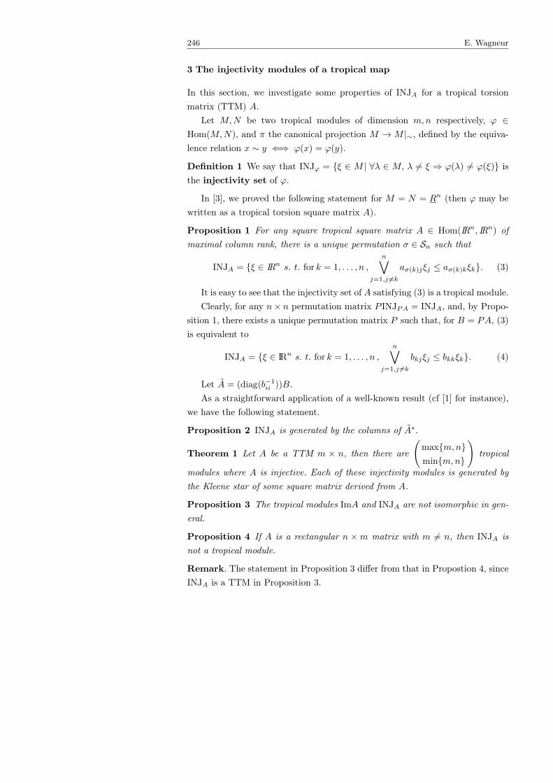
246 E. Wagneur
3 The injectivity modules of a tropical map
In this section, we investigate some properties of INJA for a tropical torsionmatrix (TTM) A.
Let M,N be two tropical modules of dimension m,n respectively, ϕ ∈Hom(M,N), and π the canonical projection M → M |∼, defined by the equiva-lence relation x ∼ y ⇐⇒ ϕ(x) = ϕ(y).
Definition 1 We say that INJϕ = ξ ∈ M | ∀λ ∈ M, λ 6= ξ ⇒ ϕ(λ) 6= ϕ(ξ) isthe injectivity set of ϕ.
In [3], we proved the following statement for M = N = Rn (then ϕ may bewritten as a tropical torsion square matrix A).
Proposition 1 For any square tropical square matrix A ∈ Hom(IRn, IRn) ofmaximal column rank, there is a unique permutation σ ∈ Sn such that
INJA = ξ ∈ IRn s. t. for k = 1, . . . , n ,
n∨j=1,j 6=k
aσ(k)jξj ≤ aσ(k)kξk. (3)
It is easy to see that the injectivity set of A satisfying (3) is a tropical module.Clearly, for any n× n permutation matrix P INJPA = INJA, and, by Propo-
sition 1, there exists a unique permutation matrix P such that, for B = PA, (3)is equivalent to
INJA = ξ ∈ IRn s. t. for k = 1, . . . , n ,
n∨j=1,j 6=k
bkjξj ≤ bkkξk. (4)
Let A = (diag(b−1ii ))B.As a straightforward application of a well-known result (cf [1] for instance),
we have the following statement.
Proposition 2 INJA is generated by the columns of A∗.
Theorem 1 Let A be a TTM m × n, then there are
(maxm,nminm,n
)tropical
modules where A is injective. Each of these injectivity modules is generated bythe Kleene star of some square matrix derived from A.
Proposition 3 The tropical modules ImA and INJA are not isomorphic in gen-eral.
Proposition 4 If A is a rectangular n ×m matrix with m 6= n, then INJA isnot a tropical module.
Remark. The statement in Proposition 3 differ from that in Propostion 4, sinceINJA is a TTM in Proposition 3.
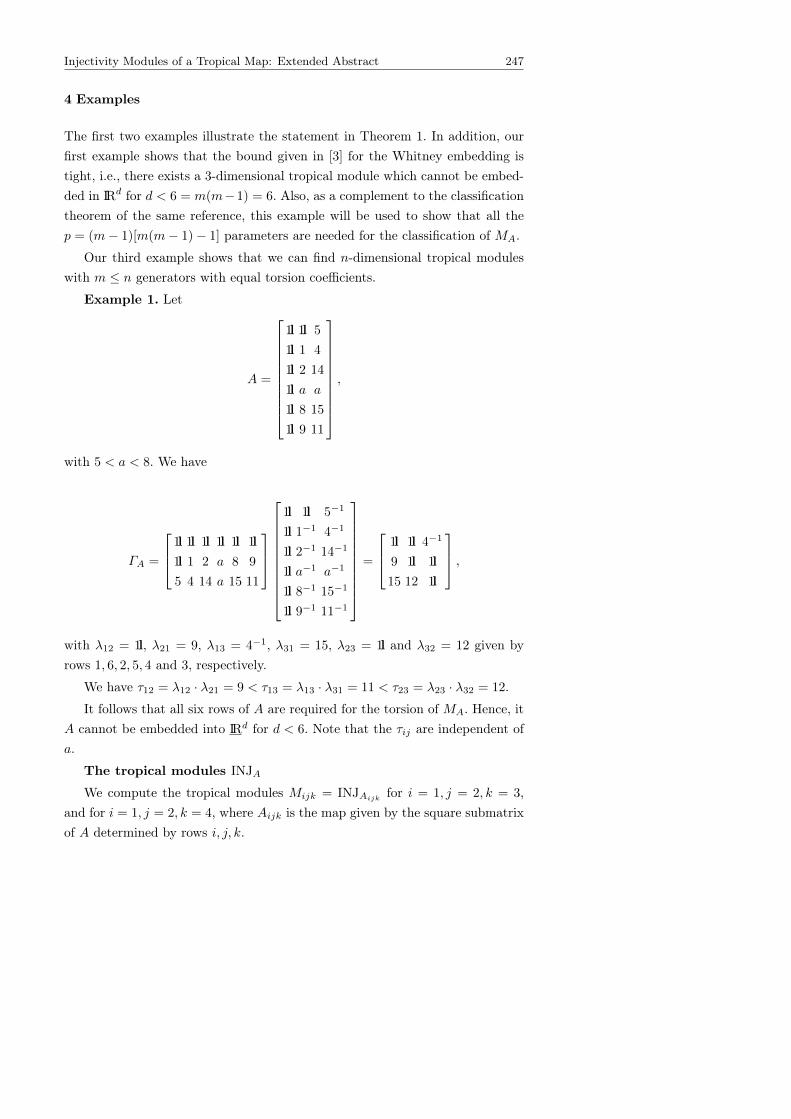
Injectivity Modules of a Tropical Map: Extended Abstract 247
4 Examples
The first two examples illustrate the statement in Theorem 1. In addition, ourfirst example shows that the bound given in [3] for the Whitney embedding istight, i.e., there exists a 3-dimensional tropical module which cannot be embed-ded in IRd for d < 6 = m(m−1) = 6. Also, as a complement to the classificationtheorem of the same reference, this example will be used to show that all thep = (m− 1)[m(m− 1)− 1] parameters are needed for the classification of MA.
Our third example shows that we can find n-dimensional tropical moduleswith m ≤ n generators with equal torsion coefficients.
Example 1. Let
A =
1l 1l 5
1l 1 4
1l 2 14
1l a a
1l 8 15
1l 9 11
,
with 5 < a < 8. We have
ΓA =
1l 1l 1l 1l 1l 1l1l 1 2 a 8 9
5 4 14 a 15 11
1l 1l 5−1
1l 1−1 4−1
1l 2−1 14−1
1l a−1 a−1
1l 8−1 15−1
1l 9−1 11−1
=
1l 1l 4−1
9 1l 1l15 12 1l
,
with λ12 = 1l, λ21 = 9, λ13 = 4−1, λ31 = 15, λ23 = 1l and λ32 = 12 given byrows 1, 6, 2, 5, 4 and 3, respectively.
We have τ12 = λ12 · λ21 = 9 < τ13 = λ13 · λ31 = 11 < τ23 = λ23 · λ32 = 12.
It follows that all six rows of A are required for the torsion of MA. Hence, itA cannot be embedded into IRd for d < 6. Note that the τij are independent ofa.
The tropical modules INJA
We compute the tropical modules Mijk = INJAijkfor i = 1, j = 2, k = 3,
and for i = 1, j = 2, k = 4, where Aijk is the map given by the square submatrixof A determined by rows i, j, k.
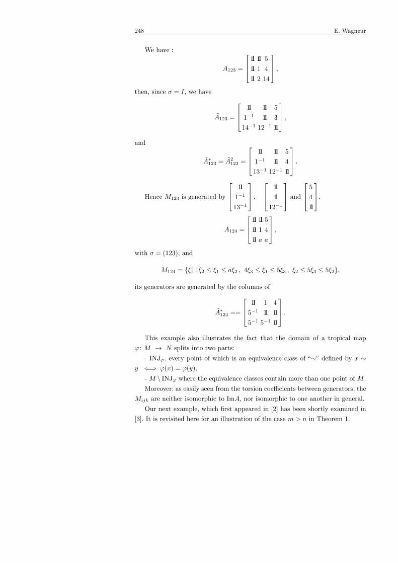
248 E. Wagneur
We have :
A123 =
1l 1l 5
1l 1 4
1l 2 14
,then, since σ = I, we have
A123 =
1l 1l 5
1−1 1l 3
14−1 12−1 1l
,and
A∗123 = A2123 =
1l 1l 5
1−1 1l 4
13−1 12−1 1l
.
Hence M123 is generated by
1l1−1
13−1
, 1l
1l12−1
and
5
4
1l
.
A124 =
1l 1l 51l 1 4
1l a a
,with σ = (123), and
M124 = ξ| 1ξ2 ≤ ξ1 ≤ aξ2 , 4ξ3 ≤ ξ1 ≤ 5ξ3 , ξ2 ≤ 5ξ3 ≤ 5ξ2,
its generators are generated by the columns of
A∗124 ==
1l 1 4
5−1 1l 1l5−1 5−1 1l
.This example also illustrates the fact that the domain of a tropical map
ϕ : M → N splits into two parts:- INJϕ, every point of which is an equivalence class of “∼” defined by x ∼
y ⇐⇒ ϕ(x) = ϕ(y),- M \ INJϕ where the equivalence classes contain more than one point of M .Moreover: as easily seen from the torsion coefficients between generators, the
Mijk are neither isomorphic to ImA, nor isomorphic to one another in general.Our next example, which first appeared in [2] has been shortly examined in
[3]. It is revisited here for an illustration of the case m > n in Theorem 1.
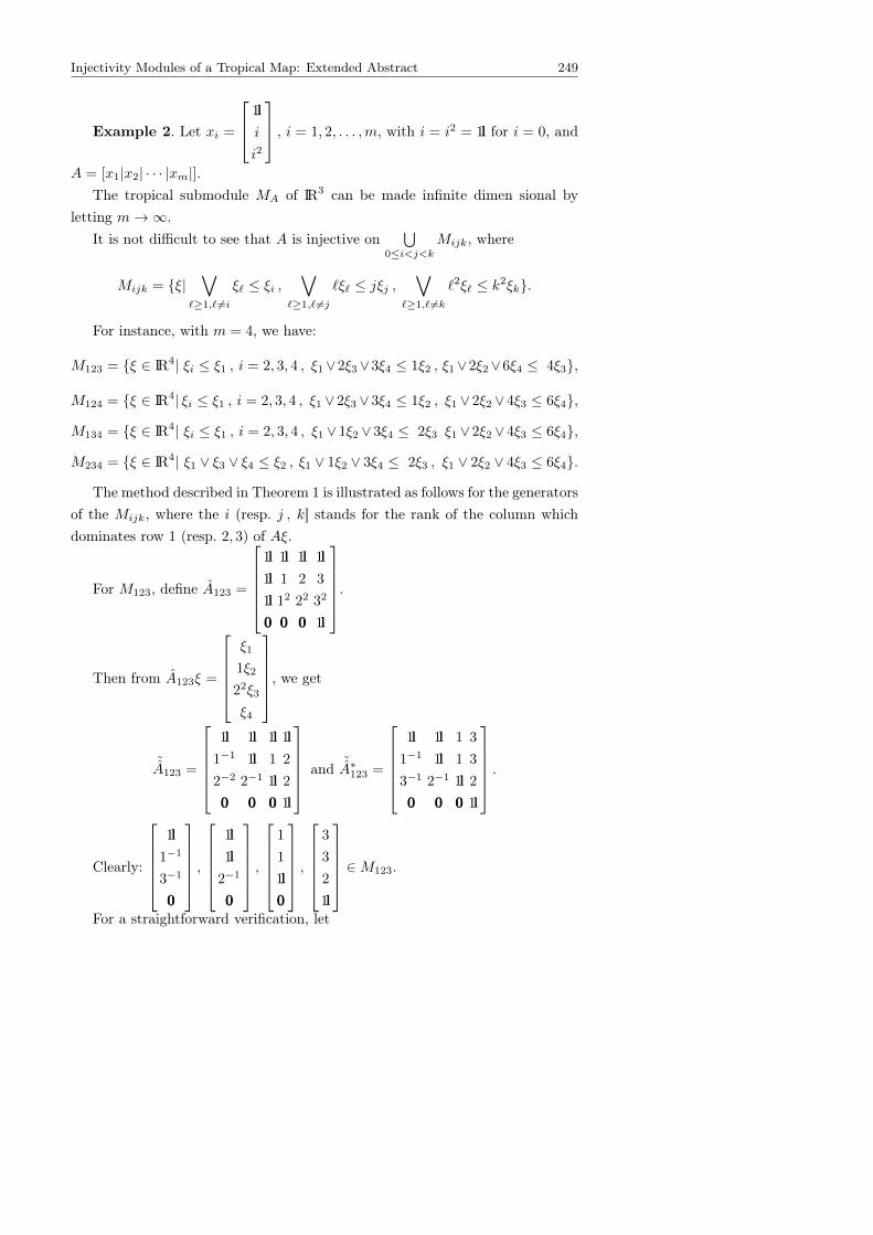
Injectivity Modules of a Tropical Map: Extended Abstract 249
Example 2. Let xi =
1li
i2
, i = 1, 2, . . . ,m, with i = i2 = 1l for i = 0, and
A = [x1|x2| · · · |xm|].The tropical submodule MA of IR3 can be made infinite dimen sional by
letting m→∞.It is not difficult to see that A is injective on
⋃0≤i<j<k
Mijk, where
Mijk = ξ|∨
`≥1, 6=i
ξ` ≤ ξi ,∨
`≥1, 6=j
`ξ` ≤ jξj ,∨
`≥1, 6=k
`2ξ` ≤ k2ξk.
For instance, with m = 4, we have:
M123 = ξ ∈ IR4| ξi ≤ ξ1 , i = 2, 3, 4 , ξ1∨2ξ3∨3ξ4 ≤ 1ξ2 , ξ1∨2ξ2∨6ξ4 ≤ 4ξ3,
M124 = ξ ∈ IR4| ξi ≤ ξ1 , i = 2, 3, 4 , ξ1 ∨ 2ξ3 ∨ 3ξ4 ≤ 1ξ2 , ξ1 ∨ 2ξ2 ∨ 4ξ3 ≤ 6ξ4,
M134 = ξ ∈ IR4| ξi ≤ ξ1 , i = 2, 3, 4 , ξ1 ∨ 1ξ2 ∨ 3ξ4 ≤ 2ξ3 ξ1 ∨ 2ξ2 ∨ 4ξ3 ≤ 6ξ4,
M234 = ξ ∈ IR4| ξ1 ∨ ξ3 ∨ ξ4 ≤ ξ2 , ξ1 ∨ 1ξ2 ∨ 3ξ4 ≤ 2ξ3 , ξ1 ∨ 2ξ2 ∨ 4ξ3 ≤ 6ξ4.
The method described in Theorem 1 is illustrated as follows for the generatorsof the Mijk, where the i (resp. j , k] stands for the rank of the column whichdominates row 1 (resp. 2, 3) of Aξ.
For M123, define A123 =
1l 1l 1l 1l1l 1 2 3
1l 12 22 32
000 000 000 1l
.
Then from A123ξ =
ξ1
1ξ2
22ξ3
ξ4
, we get
˜A123 =
1l 1l 1l 1l1−1 1l 1 2
2−2 2−1 1l 2000 000 000 1l
and ˜A∗123 =
1l 1l 1 3
1−1 1l 1 3
3−1 2−1 1l 2000 000 000 1l
.
Clearly:
1l1−1
3−1
000
,
1l1l2−1
000
,1
1
1l000
,3
3
2
1l
∈M123.
For a straightforward verification, let
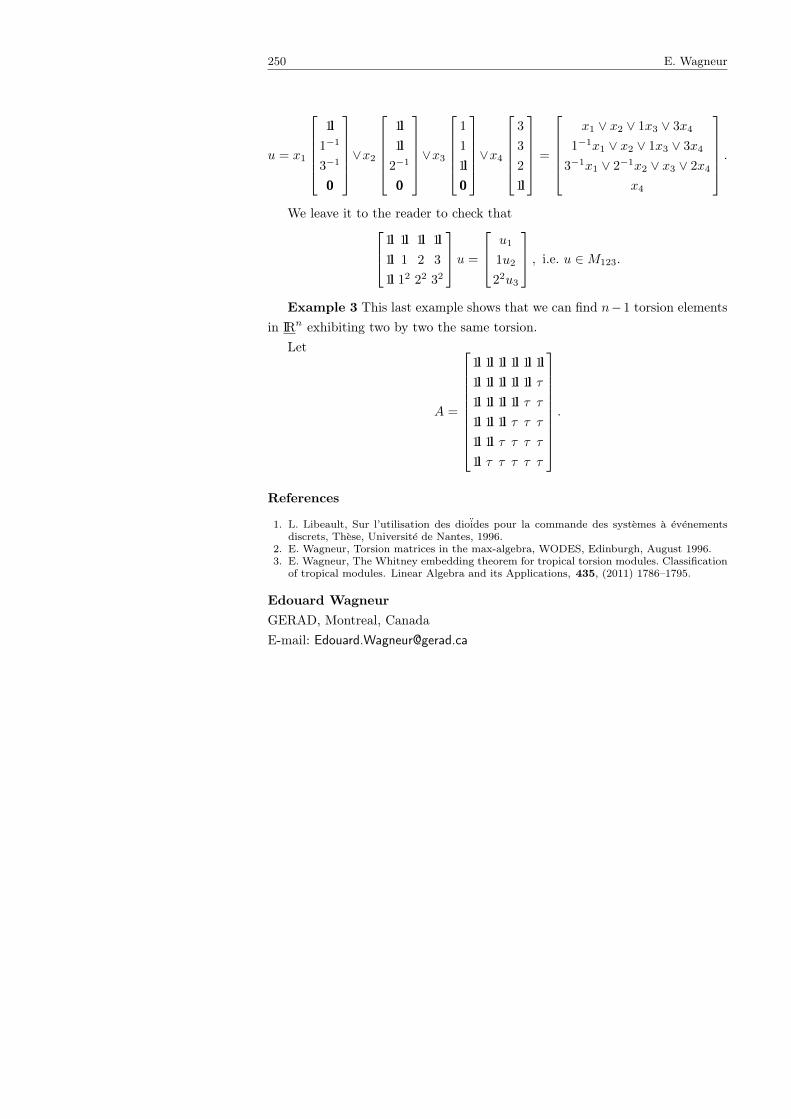
250 E. Wagneur
u = x1
1l1−1
3−1
000
∨x2
1l1l2−1
000
∨x31
1
1l000
∨x43
3
2
1l
=
x1 ∨ x2 ∨ 1x3 ∨ 3x4
1−1x1 ∨ x2 ∨ 1x3 ∨ 3x4
3−1x1 ∨ 2−1x2 ∨ x3 ∨ 2x4
x4
.We leave it to the reader to check that1l 1l 1l 1l
1l 1 2 3
1l 12 22 32
u =
u1
1u2
22u3
, i.e. u ∈M123.
Example 3 This last example shows that we can find n−1 torsion elementsin IRn exhibiting two by two the same torsion.
Let
A =
1l 1l 1l 1l 1l 1l1l 1l 1l 1l 1l τ1l 1l 1l 1l τ τ1l 1l 1l τ τ τ1l 1l τ τ τ τ1l τ τ τ τ τ
.
References
1. L. Libeault, Sur l’utilisation des dioides pour la commande des systemes a evenementsdiscrets, These, Universite de Nantes, 1996.
2. E. Wagneur, Torsion matrices in the max-algebra, WODES, Edinburgh, August 1996.3. E. Wagneur, The Whitney embedding theorem for tropical torsion modules. Classification
of tropical modules. Linear Algebra and its Applications, 435, (2011) 1786–1795.
Edouard WagneurGERAD, Montreal, CanadaE-mail: [email protected]
Tropical and Idempotent Mathematics. Moscow, Russia, August 26–31, 2012
Studying isometry groups using the horofunctionboundary
Cormac Walsh
The horofunction boundary was introduced by Gromov [13] in the late 1970sbut did not receive much study until recently. It has applications in studyingisometry groups [16], random walks [15], quantum metric spaces [21], and is agood setting for Patterson–Sullivan measures [4].
To define this boundary for a metric space (X, d), one identifies each pointx with the function d(·, x) − d(b, x), where b is some arbitrary basepoint, andthen takes the closure of the set of these functions with respect to some functionspace topology, usually the topology of uniform convergence on bounded sets.Under appropriate conditions, this gives a compactification of the metric space,and one defines the horofunction boundary to be the closure minus the originalset of functions. Elements of this boundary are called horofunctions.
This boundary is not the same as the better known Gromov boundary ofa δ-hyperbolic space. For these spaces, it has been shown [5, 23, 32] that thehorofunction boundary is finer than the Gromov boundary in the sense thatthere exists a continuous surjection from the former to the latter.
A particularly interesting subset of the horofunction boundary is the set ofthose horofunctions that are the limits of almost-geodesics. An almost-geodesic,as defined by Rieffel [21], is a map γ from an unbounded set T ⊂ R+ containing0 to X, such that for any ε > 0,
|d(γ(0), γ(s)) + d(γ(s), γ(t))− t| < ε
for all t ∈ T and s ∈ T large enough with t ≥ s. Rieffel called the limits of suchpaths Busemann points.
252 C. Walsh
As noted by Ballmann [2], the construction above is an additive analogueof the way the Martin boundary is constructed in Probabilistic Potential The-ory. One may pursue the analogy further in the framework of max-plus algebra,where one replaces the usual operations of addition and multiplication by thoseof maximum and addition. Indeed, this approach has already provided inspira-tion for many results about the horofunction boundary [1, 29]. We mention, forexample, the characterisation of Busemann points as the functions in the horo-function boundary that are extremal generators in the max-plus sense of the setof 1-Lipschitz functions. So the set of Busemann points is seen to be an analogueof the minimal Martin boundary. There is also a representation of 1-Lipschitzfunctions in terms of horofunctions analogous to the Martin representation the-orem.
The first metric spaces for which the horofunction boundary was investigatedwere those of Hadamard manifolds [3] and Hadamard spaces [2], where the ho-rofunction boundary turns out to be homeomorphic to the ray boundary andall horofunctions are Busemann points. The case of finite-dimensional normedspaces has also been studied, by Karlsson et. al. when the norm is polyhedral [14],and more generally by the present author [26]. More examples include variousfinitely-generated groups with their word metrics [7,28,31] and Finsler p–metricson GL(n,C)/Un [11, 12]. Webster and Winchester have some general results onwhen all horofunctions are Busemann points [33].
The action of the isometry group of a metric space extends continuously toan action by homeomorphisms on the horofunction boundary. Thus, the horo-function boundary is useful for studying groups of isometries of metric spaces. Inparticular, one of the tools it provides is the detour metric, which is a (possiblyinfinite valued) metric on the set of Busemann points. One may define it as thesymmetrisation of the detour cost
H(ξ, η) = infγ
lim inft→∞
(d(b, γ(t)) + η(γ(t))
).
Here, ξ and η are horofunctions, and the infimum is taken over all paths γ :
R+ → X converging to ξ. This concept appears first in [1].
In the following sections, we describe in more detail how the horofunctionboundary may be used to investigate the isometry groups of particular metricspaces.
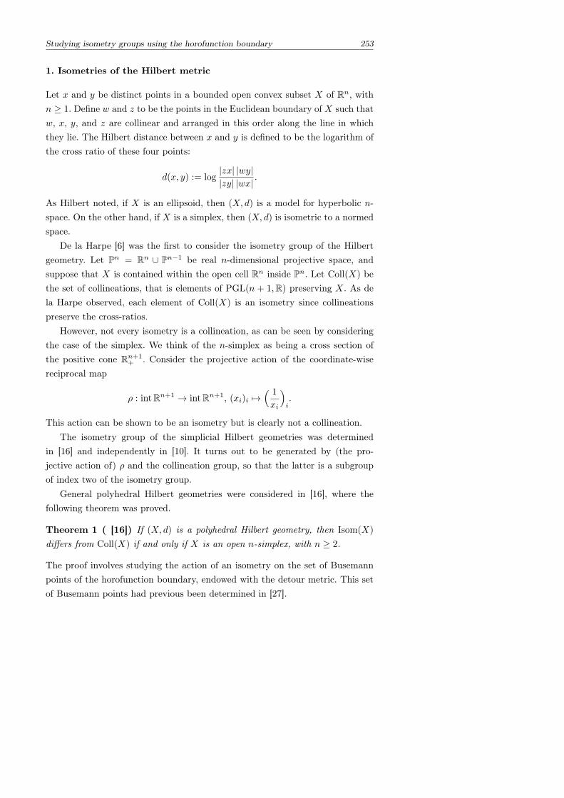
Studying isometry groups using the horofunction boundary 253
1. Isometries of the Hilbert metric
Let x and y be distinct points in a bounded open convex subset X of Rn, withn ≥ 1. Define w and z to be the points in the Euclidean boundary of X such thatw, x, y, and z are collinear and arranged in this order along the line in whichthey lie. The Hilbert distance between x and y is defined to be the logarithm ofthe cross ratio of these four points:
d(x, y) := log|zx| |wy||zy| |wx|
.
As Hilbert noted, if X is an ellipsoid, then (X, d) is a model for hyperbolic n-space. On the other hand, if X is a simplex, then (X, d) is isometric to a normedspace.
De la Harpe [6] was the first to consider the isometry group of the Hilbertgeometry. Let Pn = Rn ∪ Pn−1 be real n-dimensional projective space, andsuppose that X is contained within the open cell Rn inside Pn. Let Coll(X) bethe set of collineations, that is elements of PGL(n + 1,R) preserving X. As dela Harpe observed, each element of Coll(X) is an isometry since collineationspreserve the cross-ratios.
However, not every isometry is a collineation, as can be seen by consideringthe case of the simplex. We think of the n-simplex as being a cross section ofthe positive cone Rn+1
+ . Consider the projective action of the coordinate-wisereciprocal map
ρ : intRn+1 → intRn+1, (xi)i 7→( 1
xi
)i.
This action can be shown to be an isometry but is clearly not a collineation.The isometry group of the simplicial Hilbert geometries was determined
in [16] and independently in [10]. It turns out to be generated by (the pro-jective action of) ρ and the collineation group, so that the latter is a subgroupof index two of the isometry group.
General polyhedral Hilbert geometries were considered in [16], where thefollowing theorem was proved.
Theorem 1 ( [16]) If (X, d) is a polyhedral Hilbert geometry, then Isom(X)
differs from Coll(X) if and only if X is an open n-simplex, with n ≥ 2.
The proof involves studying the action of an isometry on the set of Busemannpoints of the horofunction boundary, endowed with the detour metric. This setof Busemann points had previous been determined in [27].
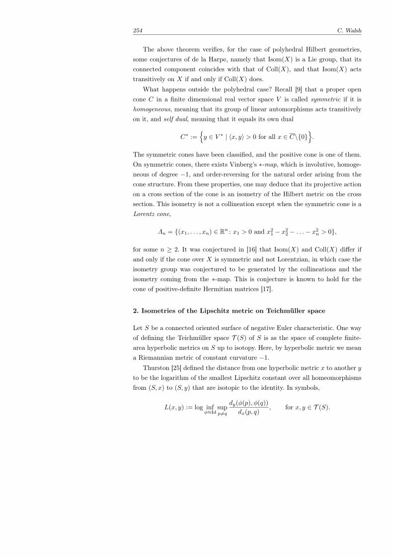
254 C. Walsh
The above theorem verifies, for the case of polyhedral Hilbert geometries,some conjectures of de la Harpe, namely that Isom(X) is a Lie group, that itsconnected component coincides with that of Coll(X), and that Isom(X) actstransitively on X if and only if Coll(X) does.
What happens outside the polyhedral case? Recall [9] that a proper opencone C in a finite dimensional real vector space V is called symmetric if it ishomogeneous, meaning that its group of linear automorphisms acts transitivelyon it, and self dual, meaning that it equals its own dual
C∗ :=y ∈ V ∗ | 〈x, y〉 > 0 for all x ∈ C\0
.
The symmetric cones have been classified, and the positive cone is one of them.On symmetric cones, there exists Vinberg’s ∗-map, which is involutive, homoge-neous of degree −1, and order-reversing for the natural order arising from thecone structure. From these properties, one may deduce that its projective actionon a cross section of the cone is an isometry of the Hilbert metric on the crosssection. This isometry is not a collineation except when the symmetric cone is aLorentz cone,
Λn = (x1, . . . , xn) ∈ Rn : x1 > 0 and x21 − x22 − . . .− x2n > 0,
for some n ≥ 2. It was conjectured in [16] that Isom(X) and Coll(X) differ ifand only if the cone over X is symmetric and not Lorentzian, in which case theisometry group was conjectured to be generated by the collineations and theisometry coming from the ∗-map. This is conjecture is known to hold for thecone of positive-definite Hermitian matrices [17].
2. Isometries of the Lipschitz metric on Teichmuller space
Let S be a connected oriented surface of negative Euler characteristic. One wayof defining the Teichmuller space T (S) of S is as the space of complete finite-area hyperbolic metrics on S up to isotopy. Here, by hyperbolic metric we meana Riemannian metric of constant curvature −1.
Thurston [25] defined the distance from one hyperbolic metric x to another yto be the logarithm of the smallest Lipschitz constant over all homeomorphismsfrom (S, x) to (S, y) that are isotopic to the identity. In symbols,
L(x, y) := log infφ≈Id
supp 6=q
dy(φ(p), φ(q))
dx(p, q), for x, y ∈ T (S).
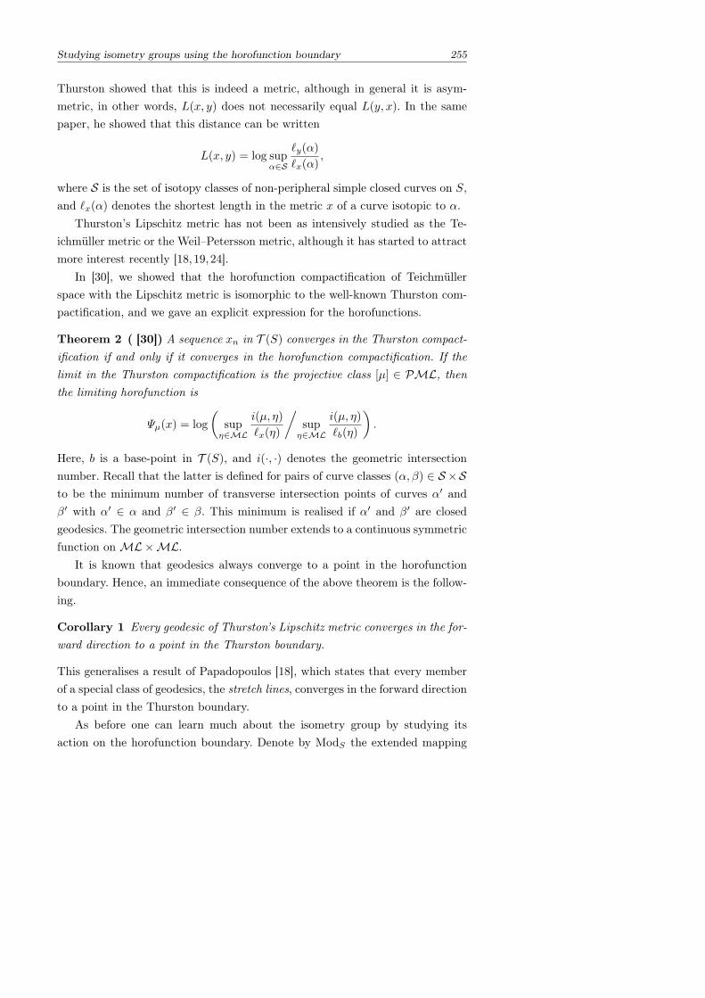
Studying isometry groups using the horofunction boundary 255
Thurston showed that this is indeed a metric, although in general it is asym-metric, in other words, L(x, y) does not necessarily equal L(y, x). In the samepaper, he showed that this distance can be written
L(x, y) = log supα∈S
`y(α)
`x(α),
where S is the set of isotopy classes of non-peripheral simple closed curves on S,and `x(α) denotes the shortest length in the metric x of a curve isotopic to α.
Thurston’s Lipschitz metric has not been as intensively studied as the Te-ichmuller metric or the Weil–Petersson metric, although it has started to attractmore interest recently [18,19,24].
In [30], we showed that the horofunction compactification of Teichmullerspace with the Lipschitz metric is isomorphic to the well-known Thurston com-pactification, and we gave an explicit expression for the horofunctions.
Theorem 2 ( [30]) A sequence xn in T (S) converges in the Thurston compact-ification if and only if it converges in the horofunction compactification. If thelimit in the Thurston compactification is the projective class [µ] ∈ PML, thenthe limiting horofunction is
Ψµ(x) = log
(supη∈ML
i(µ, η)
`x(η)
/supη∈ML
i(µ, η)
`b(η)
).
Here, b is a base-point in T (S), and i(·, ·) denotes the geometric intersectionnumber. Recall that the latter is defined for pairs of curve classes (α, β) ∈ S ×Sto be the minimum number of transverse intersection points of curves α′ andβ′ with α′ ∈ α and β′ ∈ β. This minimum is realised if α′ and β′ are closedgeodesics. The geometric intersection number extends to a continuous symmetricfunction onML×ML.
It is known that geodesics always converge to a point in the horofunctionboundary. Hence, an immediate consequence of the above theorem is the follow-ing.
Corollary 1 Every geodesic of Thurston’s Lipschitz metric converges in the for-ward direction to a point in the Thurston boundary.
This generalises a result of Papadopoulos [18], which states that every memberof a special class of geodesics, the stretch lines, converges in the forward directionto a point in the Thurston boundary.
As before one can learn much about the isometry group by studying itsaction on the horofunction boundary. Denote by ModS the extended mapping
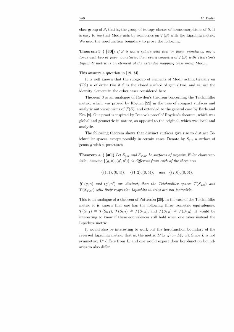
256 C. Walsh
class group of S, that is, the group of isotopy classes of homeomorphisms of S. Itis easy to see that ModS acts by isometries on T (S) with the Lipschitz metric.We used the horofunction boundary to prove the following.
Theorem 3 ( [30]) If S is not a sphere with four or fewer punctures, nor atorus with two or fewer punctures, then every isometry of T (S) with Thurston’sLipschitz metric is an element of the extended mapping class group ModS.
This answers a question in [19, §4].
It is well known that the subgroup of elements of ModS acting trivially onT (S) is of order two if S is the closed surface of genus two, and is just theidentity element in the other cases considered here.
Theorem 3 is an analogue of Royden’s theorem concerning the Teichmullermetric, which was proved by Royden [22] in the case of compact surfaces andanalytic automorphisms of T (S), and extended to the general case by Earle andKra [8]. Our proof is inspired by Ivanov’s proof of Royden’s theorem, which wasglobal and geometric in nature, as opposed to the original, which was local andanalytic.
The following theorem shows that distinct surfaces give rise to distinct Te-ichmuller spaces, except possibly in certain cases. Denote by Sg,n a surface ofgenus g with n punctures.
Theorem 4 ( [30]) Let Sg,n and Sg′,n′ be surfaces of negative Euler character-istic. Assume (g, n), (g′, n′) is different from each of the three sets
(1, 1), (0, 4), (1, 2), (0, 5), and (2, 0), (0, 6).
If (g, n) and (g′, n′) are distinct, then the Teichmuller spaces T (Sg,n) andT (Sg′,n′) with their respective Lipschitz metrics are not isometric.
This is an analogue of a theorem of Patterson [20]. In the case of the Teichmullermetric it is known that one has the following three isometric equivalences:T (S1,1) ∼= T (S0,4), T (S1,2) ∼= T (S0,5), and T (S2,0) ∼= T (S0,6). It would beinteresting to know if these equivalences still hold when one takes instead theLipschitz metric.
It would also be interesting to work out the horofunction boundary of thereversed Lipschitz metric, that is, the metric L∗(x, y) := L(y, x). Since L is notsymmetric, L∗ differs from L, and one would expect their horofunction bound-aries to also differ.
Studying isometry groups using the horofunction boundary 257
References
1. Marianne Akian, Stephane Gaubert, and Cormac Walsh. The max-plus Martin boundary.Doc. Math., 14:195–240, 2009.
2. Werner Ballmann. Lectures on spaces of nonpositive curvature, volume 25 of DMV Sem-inar. Birkhauser Verlag, Basel, 1995. With an appendix by Misha Brin.
3. Werner Ballmann, Mikhael Gromov, and Viktor Schroeder. Manifolds of nonpositive cur-vature, volume 61 of Progress in Mathematics. Birkhauser Boston Inc., Boston, MA, 1985.
4. M. Burger and S. Mozes. CAT(-1)-spaces, divergence groups and their commensurators.J. Amer. Math. Soc., 9(1):57–93, 1996.
5. Michel Coornaert and Athanase Papadopoulos. Horofunctions and symbolic dynamics onGromov hyperbolic groups. Glasg. Math. J., 43(3):425–456, 2001.
6. Pierre de la Harpe. On Hilbert’s metric for simplices. In Geometric group theory, Vol.1 (Sussex, 1991), volume 181 of London Math. Soc. Lecture Note Ser., pages 97–119.Cambridge Univ. Press, Cambridge, 1993.
7. Mike Develin. Cayley compactifications of abelian groups. Ann. Comb., 6(3-4):295–312,2002.
8. Clifford J. Earle and Irwin Kra. On isometries between Teichmuller spaces. Duke Math.J., 41:583–591, 1974.
9. Jacques Faraut and Adam Koranyi. Analysis on symmetric cones. Oxford MathematicalMonographs. The Clarendon Press Oxford University Press, New York, 1994. OxfordScience Publications.
10. Stefano Francaviglia and Armando Martino. The isometry group of Outer Space, 2009.Preprint. arXiv:0912.0299.
11. Shmuel Friedland and Pedro J. Freitas. p-metrics on GL(n,C)/Un and their Busemanncompactifications. Linear Algebra Appl., 376:1–18, 2004.
12. Shmuel Friedland and Pedro J. Freitas. Revisiting the Siegel upper half plane. I. LinearAlgebra Appl., 376:19–44, 2004.
13. M. Gromov. Hyperbolic manifolds, groups and actions. In Riemann surfaces and relatedtopics: Proceedings of the 1978 Stony Brook Conference (State Univ. New York, StonyBrook, N.Y., 1978), volume 97 of Ann. of Math. Stud., pages 183–213, Princeton, N.J.,1981. Princeton Univ. Press.
14. A. Karlsson, V. Metz, and G. Noskov. Horoballs in simplices and Minkowski spaces. Int.J. Math. Math. Sci., 2006. Art. ID 23656, 20 pages.
15. Anders Karlsson and Francois Ledrappier. On laws of large numbers for random walks.Ann. Probab., 34(5):1693–1706, 2006.
16. Bas Lemmens and Cormac Walsh. Isometries of polyhedral Hilbert geometries. J. Topol.Anal., 3(2):213–241, 2011.
17. Lajos Molnar. Thompson isometries of the space of invertible positive operators. Proc.Amer. Math. Soc., 137(11):3849–3859, 2009.
18. Athanase Papadopoulos. On Thurston’s boundary of Teichmuller space and the extensionof earthquakes. Topology Appl., 41(3):147–177, 1991.
19. Athanase Papadopoulos and Guillaume Theret. On Teichmuller’s metric and Thurston’sasymmetric metric on Teichmuller space. In Handbook of Teichmuller theory. Vol. I,volume 11 of IRMA Lect. Math. Theor. Phys., pages 111–204. Eur. Math. Soc., Zurich,2007.
20. David B. Patterson. The Teichmuller spaces are distinct. Proc. Amer. Math. Soc., 35:179–182, 1972.
21. Marc A. Rieffel. Group C∗-algebras as compact quantum metric spaces. Doc. Math.,7:605–651 (electronic), 2002.
22. H. L. Royden. Automorphisms and isometries of Teichmuller space. In Advances in theTheory of Riemann Surfaces (Proc. Conf., Stony Brook, N.Y., 1969), pages 369–383.Ann. of Math. Studies, No. 66. Princeton Univ. Press, Princeton, N.J., 1971.
23. Peter A. Storm. The barycenter method on singular spaces. Comment. Math. Helv.,82(1):133–173, 2007.
24. Guillaume Theret. A propos de la metrique asymetrique de Thurston sur l’espace de Te-ichmuller d’une surface. Prepublication de l’Institut de Recherche Mathematique Avancee[Prepublication of the Institute of Advanced Mathematical Research], 2005/8. UniversiteLouis Pasteur. Institut de Recherche Mathematique Avancee, Strasbourg, 2005. These,Universite Louis Pasteur (Strasbourg I), Strasbourg, 2005.
25. William Thurston. Minimal stretch maps between hyperbolic surfaces. preprint,arXiv:math GT/9801039, 1986.
26. Cormac Walsh. The horofunction boundary of finite-dimensional normed spaces. Math.Proc. Cambridge Philos. Soc., 142(3):497–507, 2007.
27. Cormac Walsh. The horofunction boundary of the Hilbert geometry. Adv. Geom.,8(4):503–529, 2008.
28. Cormac Walsh. Busemann points of Artin groups of dihedral type. Internat. J. AlgebraComput., 19(7):891–910, 2009.
29. Cormac Walsh. Minimum representing measures in idempotent analysis. In Tropical andidempotent mathematics, volume 495 of Contemp. Math., pages 367–382. Amer. Math.Soc., Providence, RI, 2009.
30. Cormac Walsh. The horoboundary and isometry group of Thurston’s Lipschitz Metric,2010. arXiv:1006.2158v1.
31. Cormac Walsh. The action of a nilpotent group on its horofunction boundary has finiteorbits. Groups Geom. Dyn., 5(1):189–206, 2011.
32. Corran Webster and Adam Winchester. Boundaries of hyperbolic metric spaces. PacificJ. Math., 221(1):147–158, 2005.
33. Corran Webster and Adam Winchester. Busemann points of infinite graphs. Trans. Amer.Math. Soc., 358(9):4209–4224 (electronic), 2006.
This work is partially supported by the joint RFBR-CNRS grant 11-01—93106-a.
Cormac WalshINRIA Saclay & Centre de Mathematiques Appliques, Ecole Polytechnique,91128 Palaiseau, FranceE-mail: [email protected]
Tropical and Idempotent Mathematics. Moscow, Russia, August 26–31, 2012
Properties of systems of (max,+)− and(max,min)−linear equations and inequalities
Karel Zimmermann
1. Introduction
Properties of systems of (max,+)-linear inequalities or equations were studiedin the literature, e.g., in [2], [3], [5], [7], [8]. The authors studied mostly eitherequations and inequalities with variables on only one-side of the equations orinequalities (we will call them "one-sided") or systems with variables on bothsides of the relations (we will call them "two-sided") with a special form of oneof the sides (e.g. when problems of (max,+)-eigenvalues and eigenvectors werestudied). The aim of the contribution is a presentation of some useful propertiesof systems (max,+)- and (max,min)-linear equations and inequalities, which canbe used for a detailed analysis of solution sets of such systems. Both "one-sided"and "two-sided" systems will be considered.
Problems on algebraic structures, in which pairs of operations (max,+) or(max,min) replace addition and multiplication of the classical linear algebra,have appeared in the literature approximately since the sixties of the last cen-tury (see, e.g., [5], [10]). A systematic theory of such algebraic structures waspublished, e.g., in [2], [5] [7], [8]. These works investigate, among other problems,systems of the so called (max,+)- or (max,min)-linear equations with variableson only one side of the equations. Since operation ”max ” replacing addition isno more a group operation, but only a semigroup operation, there is a substantialdifference between solving systems with variables on one side and systems withvariables occuring on both sides of equations or inequalities. The former systemswill be called "one-sided" and the latter systems "two-sided". Special two-sided
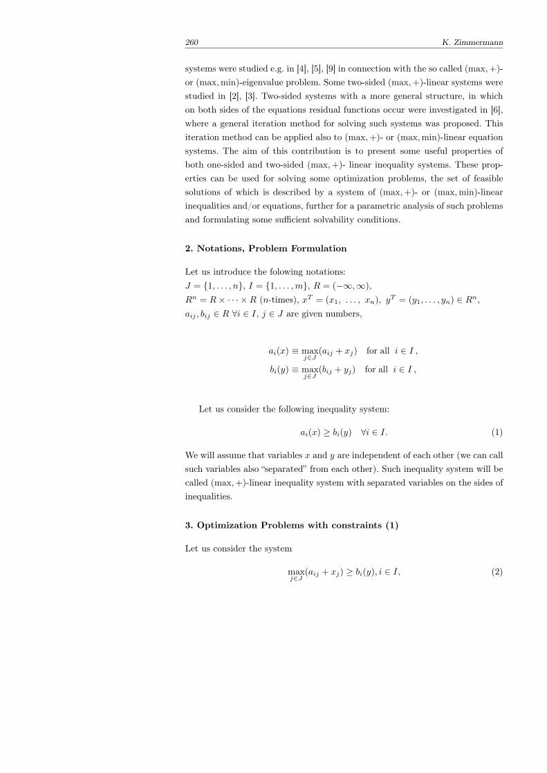
260 K. Zimmermann
systems were studied e.g. in [4], [5], [9] in connection with the so called (max,+)-or (max,min)-eigenvalue problem. Some two-sided (max,+)-linear systems werestudied in [2], [3]. Two-sided systems with a more general structure, in whichon both sides of the equations residual functions occur were investigated in [6],where a general iteration method for solving such systems was proposed. Thisiteration method can be applied also to (max,+)- or (max,min)-linear equationsystems. The aim of this contribution is to present some useful properties ofboth one-sided and two-sided (max,+)- linear inequality systems. These prop-erties can be used for solving some optimization problems, the set of feasiblesolutions of which is described by a system of (max,+)- or (max,min)-linearinequalities and/or equations, further for a parametric analysis of such problemsand formulating some sufficient solvability conditions.
2. Notations, Problem Formulation
Let us introduce the folowing notations:J = 1, . . . , n, I = 1, . . . ,m, R = (−∞,∞),Rn = R× · · · ×R (n-times), xT = (x1, . . . , xn), yT = (y1, . . . , yn) ∈ Rn,aij , bij ∈ R ∀i ∈ I, j ∈ J are given numbers,
ai(x) ≡ maxj∈J
(aij + xj) for all i ∈ I ,
bi(y) ≡ maxj∈J
(bij + yj) for all i ∈ I ,
Let us consider the following inequality system:
ai(x) ≥ bi(y) ∀i ∈ I. (1)
We will assume that variables x and y are independent of each other (we can callsuch variables also “separated” from each other). Such inequality system will becalled (max,+)-linear inequality system with separated variables on the sides ofinequalities.
3. Optimization Problems with constraints (1)
Let us consider the system
maxj∈J
(aij + xj) ≥ bi(y), i ∈ I, (2)
Properties of systems 261
and assume that variables xT = (x1, . . . , xn), yT = (y1, . . . , yn) are indepen-
dent. Let M(x.y) denote the set of all solutions of system (2).We will investigate the following optimization problem:
f(x) ≡ maxj∈J
(fj(xj)) −→ min (3)
subject to
x ∈M(x, y), (4)
where we assume that y is fixed and fj , j ∈ J are continuous increasing func-tions. Let xopt(y) be the optimal solution of problem (3), (4). Using the resultsof [11] we obtain explicit formulas for the optimal solutions of the optimizationproblem above. For this purpose we will introduce the following notations for alli ∈ I, j ∈ J :
Tij ≡ xj ; aij + xj ≥ bi(y),
fj(x(i)j (y)) = min
xj∈Tij
fj(xj),
where we set the minimum equal to ∞ if Tij = ∅. We set further:
minj∈J
(fj(x(i)j (y)) = fj(i)(x
(i)j(i)(y)),
Vj ≡ i ; j(i) = j,
Then the following theorem follows from the results contained in [11]:
Theorem 1 Let
x∗j (y) = maxi∈Vj
(bi(y)− aij) if Vj 6= ∅
x∗j (y) = −∞ if Vj = ∅
Then x∗(y) is the optimal solution of problem (3), (4).
Using this result we can derive explicit formulas for optimal solutions of theproblem for any y. If we interpret y as parameters, on which the right hand sidesof the constraint depend, post-optimal parametric analysis of the problems canbe carried out. In the same way, problems, with (max,min)-linear inequalitieswill be analyzed. More general cases of dependence on y in the right hand sideswill be investigated. Using Theorem 1 some sufficient conditions for solvability oftwo-sided (max,+)- and (max,min)-linear equation and/or inequality systemswill be presented.
262 K. Zimmermann
4. The Reachable Right Hand Sides
Let us consider the system
max(aij + xj) = bi, i ∈ I, (5)
where bT = (b1, . . . , bm) ∈ Rm. Let M(b) denote the set of all solutions ofsystem (5) for the given b. It is well-known that if M(b) 6= ∅, then there existsalways the maximum element xmax(b) of set M(b), i.e. element xmax(b) ∈M(b)
such that x ≤ xmax(b), ∀x ∈ M(b). The maximum element of M(b) can becalculated as follows:
xmaxj = min
i∈I(bi − aij) ∀j ∈ J. (6)
The reachability set R(A) of a given matrix A with elements aij , i ∈ I, j ∈ J
is defined as follows:R(A) = b ; M(b) 6= ∅. (7)
Let us consider the system of equations for unknown b of the form:
minr∈I
(br − arj) = hj , j ∈ J, (8)
where hj = mini∈I(−aij). Let us set
Sj = k ∈ I ; hj = −akj ∀j ∈ J. (9)
Theorem 2 Let us setbk = 0 ∀k ∈
⋃j∈J
Sj ,
bk = maxj∈J
(hj + akj) ∀k ∈ I \⋃j∈J
Sj .
Then b ∈ R(A).
Properties of b and of the corresponding maximum solution xmax(b) will bestudied. Some implications of the properties for solving two-sided (max,+)- and(max,min)-linear equation systems will be discussed.
We illustrate Theorem 2 by the following small numerical example.
Example 1 Let us consider the matrix
A =
4 3 1
2 −5 0
8 7 1
A∗ ≡ −AT =
−4 −2 −8−3 5 −7−1 0 −1
We have:
S1 = 3, S2 = 3, S3 = 1, 3,⋃j∈J
Sj = 1, 3, 2 6∈⋃j∈J
Sj
Following Theorem 2 we obtain:
b1 = b3 = 0, b2 = max(−6,−12,−1) = −1.
b ∈ R(A), xmax(b) = (−8,−7,−1)T .
References
1. Baccelli, F.L., Cohen, G., Olsder, G.J., Quadrat, J.P.: Synchronization and Linearity, AnAlgebra for Discrete Event Systems, Wiley, Chichester, 1992.
2. Butkovic, P.: Max-linear Systems: Theory and Algorithms, Monographs in Mathematics,Springer Verlag 2010, 271 p.
3. Butkovic, P., Hegedus, G.: An Elimination Method for Finding All Solutions of the Systemof Linear Equations over an Extremal Algebra, Ekonomicko - matematicky obzor 20 (1984),No. 2, pp. 203-215.
4. Cechlarova, K.: Efficient Computation of the Greatest Eigenvector in Fuzzy Algebra, TatraMt. Math. Publications, 1997, pp. 73-79.
5. Cuninghame-Green, R.A.: Minimax Algebra, Lecture Notes in Economics and Mathemat-ical Systems, 166, Springer Verlag, Berlin, 1979.
6. Cuninghame-Green, R.A., Zimmermann, K.: Equation with Residual Functions, Comment.Math. Univ. Carolinae 42(2001), 4, pp. 729-740.
7. G.L. Litvinov, V.P. Maslov, S.N. Sergeev (eds.): Idempotent and Tropical Mathematicsand Problems of Mathematical Physics, vol. I and II, Independent University, 2007.
8. V.P. Maslov, S.N. Samborskiı (eds.): Idempotent Analysis, Advances in Soviet Mathemat-ics, 13, AMS, Providence 1992.
9. Sanchez, E.: Inverses of Fuzzy Relations. Applications to Possibility Distributions andMedical Diagnosis, Fuzzy Sets and Systems, vol. 2, No 1, 1979, pp. 75 - 86.
10. Vorobjov, N.N.: Extremal Algebra of positive Matrices, Elektronische Informationsverar-beitung und Kybernetik, 3, 1967, pp. 39-71 (in Russian).
11. Zimmermann, K.: Solution of Some max-separable Optimization Problems with InequalityConstraints, Contemporary Mathematics, 377, Idempotent Mathematics and Mathemat-ical Physics pp. 363 - 370, (ed. G. L. Litvinov, V. P. Maslov) American MathematicalSociety, Providence, Rhod Island, 2003.
Supported by GA CR grant #402/09/0405.
Karel ZimmermannFaculty of Mathematics and Physics, Charles University PragueE-mail: [email protected]
Tropical and Idempotent Mathematics. Moscow, Russia, August 26–31, 2012
Семейство распараллеленных алгоритмов рас-познавания изображений, оптимизированныхдля реализации на многоядерных центральныхпроцессорах и спецвычислителях
Д.С. АксеновД.В. ЕвстигнеевА.В. Чуркин
Задача распознавания образов является одной из основных задач, реша-емых системами компьютерного зрения и интеллектуального анализа дан-ных. Несмотря на многократное увеличение быстродействия вычислитель-ных ядер на сегодняшний день эта задача по-прежнему не имеет универсаль-ного решения, удовлетворительного одновременно как по скорости работы,так и по точности распознавания.
За последние 30 лет разработано множество подходов к этой задаче, при-чем ряд специализированных алгоритмов (например, распознавание руко-писного письма) оказались весьма успешными, и нашли широкое примене-ние в технике. Большинство методов распознавания образов можно условноразделить на четыре класса:
Геометрические методы нормализации и расчета расстояния до прототи-па.Статистические методы оценивания вероятностного распределения иклассификация по правилу Байеса.Нейросетевые методы построения нейронной сети с весами, полученнымив ходе обучения на тренировочной выборке.Структурные методы построения классификационных правил.
Эффективность методов распознавания оценивается как по скоростипринятия решения, так и двумя вероятностями - вероятностью ошибочно-го распознавания и вероятностью нераспознавания. Уменьшение этих ве-
Семейство распараллеленных алгоритмов 265
роятностей обычно ведет к резкому увеличению вычислительных затрат и,следовательно, к увеличению времени принятия решения. Основной зада-чей предлагаемого семейства алгоритмов является компенсация увеличениявычислительных затрат за счет распараллеливания алгоритмов для эффек-тивного использования многоядерных процессоров и спецвычислителей. Вкачестве основных методов для распараллеливания и оптимизации рассмат-риваются следующие алгоритмы распознавания образов:
1) Метод собственных изображений - разновидность метода главных ком-понент в задаче геометрического распознавания образов. В основе мето-да лежит математическая операция вычисления собственных значенийи собственных векторов матрицы, составленной из изображений обучаю-щей базы. Соответствующая оптимизированная система алгоритмов дляпараллельного вычисления ковариационной матрицы, для поворота мат-рицы методами Гаусса-Зейделя и Якоби, определения собственных зна-чений и векторов позволяет до 25 раз ускорить реализацию метода соб-ственных изображений применительно к большим базам изображений(до 10 тысяч изображений).
2) Метод сопоставления графов - параллельная реализация сорока филь-тров Габора - свертка изображения с ядрами специального вида, позво-ляющая классифицировать графы, отвечающие наборам реперных точекизображения. Фильтры Габора обладают хорошей геометрической устой-чивостью, а именно, они устойчивы по отношению к геометрическим по-воротам, масштабированию, изменению яркости и контрастности.
3) Семейство нейросетевых методов распознавания изображений. Преиму-ществами таких методов является хорошая масштабируемость процессараспознавания, что позволяет использовать универсальные алгоритмыкак для многопроцессорных систем, так и для высокопроизводительныходноядерных вычислителях. Стандартные библиотеки нейросетевых ал-горитмов могут быть эффективно модифицированы для использованиякак в обычных многоядерных и многопроцессорных системах, так и вспецвычислителях с нейросетевой архитектурой.
В качестве примера приводится модификация алгоритма Якоби для па-раллельного вычисления собственных значений и собственных векторов, ис-пользуемых для идентификации изображений методом главных компонент.Вычислительный алгоритм разделен на три последовательные стадии, каж-дая из которых в свою очередь распараллелена: вычисление ковариантнойматрицы, модифицированный алгоритм Якоби и определение системы соб-
ственных векторов и собственных значений. За счет применения данной мо-дификации алгоритма на видеокарте с поддержкой архитектуры универ-сальных параллельных вычислений CUDA (GeForce 9600GT производствакомпании NVIDIA) наблюдается значительное увеличение скорости распо-знавания изображений. По сравнению с выполнением на одном ядре CPUPentium 4 с тактовой частотой 3 гигагерца выигрыш по скорости составляет30-40 раз для видеокарты GeForce 9600GT. Например, время для распозна-вания изображения из базы в 4000 фотографий размером 92х112 сократи-лось с 86494 мс до 2338 мс.
Дальнейшее развитие параллельных алгоритмов распознавания изобра-жений связано с увеличением универсальности использования отдельныхалгоритмических блоков, которые с небольшой модификацией могут бытьиспользованы как на высокопроизводительных неспециализированных ра-бочих станциях, так и на многоядерных вычислителях специальной ар-хитектуры. Работа выполнена при поддержке грантов РФФИ 11-01-93106-НЦНИЛ-а, 12-01-00886-а.
Список литературы
1. Г.Л. Литвинов, В.П. Маслов. Идемпотентная математика: принцип соответствия и егокомпьютерные приложения// Успехи матем. наук, 1996, т. 51, N 6, с. 1210-1211.
2. G.L. Litvinov, V.P. Maslov, A.Ya. Rodionov, A.N. Sobolevski, Universal algorithms,mathematics of semirings and parallel computations. Lecture Notes in ComputationalScience and Engineering, 2011, vol. 75, p. 63-89. See also E-print arXiv: 1005.1252(http://arXiv.org).
3. S. Singer, S. Singer, V. Novakovic, A. Uscumlic, and V. Dunnjko, Novel Modification ofParrallel Jacobi Algorithms, arXie:1008.0201v2,(2001).
4. П.П.Кольцов, Сравнительное изучение алгоритмов выделения и классификации тек-стур, Ж. вычисл. матем. и матем. физ., 51:8 (2011), 1561-1568.
5. Самаль Д.И., Старовойтов В.В. Подходы и методы распознавания людей по фотопорт-ретам, Минск, ИТК НАНБ, 1998.
Д.С. АксеновРоссия, Москва, МГТУ им. БауманаE-mail: [email protected]
Д.В. ЕвстигнеевМГТУ радиотехники, электроники, автоматикиE-mail: [email protected]
А.В. ЧуркинРоссия, Москва, МГУ им М.В.ЛомоносоваE-mail: [email protected]
Tropical and Idempotent Mathematics. Moscow, Russia, August 26–31, 2012
Оценки сложности алгоритма Григорьева длярешения тропических линейных систем
А. П. Давыдов
1 Постановка задачи
Определение 1 Тропическая линейная система — это прямоугольнаяматрицаm×n. Решение тропической линейной системы — это такая стро-ка из n элементов, что при прибавлении ее к каждой из строк матрицыполучится строка, в которой не будет строгого минимума, т.е. мини-мальный элемент в каждой строке должен встречаться хотя бы два раза.Тропическая линейная система называется разрешимой, если существуетстрока, являющаяся решением данной системы [3].
В данной статье мы будем рассматривать задачу о разрешимости целочис-ленных тропических линейных систем. Хотя в частных случаях (например,на квадратных матрицах [1]) данная задача может быть решена эффек-тивно, не известно ни одного алгоритма, для которого доказано полиноми-альное время работы в худшем случае. Известно, что эта задача лежит впересечении классов NP и coNP [3].
Предложение 1 Класс разрешимых тропических линейных систем инва-риантен относительно прибавления произвольной константы ко всем чис-лам в одной строке или в одном столбце. Более того, из решения системыпосле подобного преобразования можно получить решение исходной систе-мы, прибавив к найденному решению разность первых строк матрицы дои после преобразования.
Из этого предложения сразу же получается следующее замечание.
268 А. П. Давыдов
Замечание 1 Не умаляя общности, можно считать, что все числа вматрице системы неотрицательны.
Далее будут использоваться следующие обозначения:
– n(A) — количество строк матрицы A,– m(A) — количество столбцов матрицы A,– M(A) — максимальное число в матрице A,– R(A) — множество строк матрцы A.
Для простоты, если понятно, о какой матрице идет речь, параметр в этихобозначениях будет опускаться.
2 Алгоритм Григорьева
Один из сравнительно новых алгоритмов для решения тропических линей-ных систем — это алгоритм Григорьева. Ключевая особенность этого алго-ритма заключается в том, что в работе [3], в которой был предложен этоталгоритм, сразу же была показана как оценка, полиномиально зависящаяот размеров матрицы (но при этом полиномиальная от M , а не от logM),так и оценка, полиномиально зависящая от logM (но неполиномиально отразмеров матрицы).
Это означает, что любая серия контрпримеров, на которой будет дости-гаться неполиномиальное время работы, должна состоять из матриц неогра-ниченного размера с неограниченно большими элементами.
Приведем описание алгоритма Григорьева.Для начала заметим, что ввиду предложения 1 можно искать не решение
матрицы, а серию преобразований из добавления константы ко всем элемен-там в строке или столбце, которая приведет исходную матрицу к матрице,решением которой является нулевая строка. Далее решением системы мыбудем называть именно такую матрицу.
Для того чтобы решить систему размера m × n, решим систему размераm × (n−1), получаемую из первой системы удалением первой строки. С это-го момента будем считать, что во всех строках матрицы, кроме, возможно,первой, строгих минимумов нет.
Далее определим операцию спуска матрицы следующим образом.
1. Заведем множество столбцов J . Изначально в нем будет только одинстолбец — тот, в котором достигается минимум в первой строке.
2. Если J содержит все столбцы, то спуск невозможен, и алгоритм завер-шает работу.
Оценки сложности алгоритма решения тропических линейных систем 269
3. Если найдется строка, в которой лишь один минимум достигается настолбцах, не лежащих в J , то добавим столбец с этим минимумом в J ивернемся к шагу 2.
4. Вычтем из всех столбцов, не лежащих в J , максимальное число, длякоторого в каждой строке, все минимальные элементы которой лежат вJ , эти элементы останутся минимальными и после вычитания.
Замечание 2 Заметим, что хотя алгоритм спуска содержит некото-рую недетерминированность в порядке прибавления столбцов к множе-ству J , в пункте 4 множество J определено однозначно, т.к. максималь-ное по включению множество, построенное по правилам 1–3, единственно.
Предложение 2 Если изначально строгого минимума во всех строках,кроме первой, не было, то и после спуска его не будет.
Затем преобразуем матрицу в соответствии со следующим алгоритмом.
1. Если в первой строке нет строгого минимума, то задача решена.2. Иначе — cпустить матрицу. Если это невозможно, то решения нет, иначе
перейти к пункту 1.
В [3] показано, что временная сложность данного алгоритма составляетO(M · logM · m2 · n2). Позже также была показана оценка O(2mn · logM).
3 Улучшенная верхняя оценка
Теорема 1 (Верхняя оценка) Алгоритм Григорьева завершает работуза O(n·
(m+nn
)) операций спуска, что дает оценку на сложность алгоритма
в O(logM ·m · n2 ·(m+nn
)).
Чтобы доказать эту теорему, введем следующее определение.
Определение 2 Назовем расстоянием до строки матрицы минимальнуюитерацию, на которой она может быть добавлена к множеству J в опе-рации спуска матрицы. В случае, если строка не может быть добавлена кмножеству J , расстояние до нее положим равным бесконечности. Здесь идалее мы будем говорить, что строка содержится в множестве столбцовJ , если все столбцы, ы которых достигаются ее минимумы содержатсяв множестве J .
Обозначим расстояние до строки r через d0(r), а расстояние до строки r
после i-го спуска алгоритма Григорьева — через di(r). Обозначим муль-тимножество расстояний для всех строк матрицы A через D0(A), а соот-ветствующее мультимножество после i-го спуска алгоритма Григорьева —
270 А. П. Давыдов
через Di(A). Также будем использовать обозначения d(r) и D(A) для d0(r)и D0(A) соответственно.
Для расстояний, определенных вышеописанным образом, верна следую-щая теорема.
Теорема 2 Для любой матрицы A выполняются следующие свойства.
1. ∀n∈D(A) (|x < n|x ∈ D(A)| ≥ n− 1).2. После операции спуска алгоритма Григорьева расстояние до хотя бы
одной из строк увеличится.3. Обозначим через ri строку с минимальным di+1(r) среди всех строк,
для которых di(r) 6= di+1(r). Тогда
∀r∈R(A)((di(r) < di(ri))⇒ (di+1(r) = di(r)), (1)
∀r∈R(A)((di(r) ≥ di(ri))⇒ (di+1(r) ≥ di+1(ri)). (2)
Доказательство 1. Допустим, что данное утверждение неверно для рас-стояния n, соответствующего столбцу r. Рассмотрим операцию спуска,при которой столбец r добавляется к множеству J на итерации n. Наэтой итерации размер множества J равен n − 1, значит, найдется n − 1
столбец, расстояние до которых меньше n.2. Пусть r — строка с минимальным расстоянием после спуска среди всех
строк, у которых после операции спуска появился новый минимум.Несложно заметить, что расстояние до нее должно увеличиться.
3. Чтобы получить свойство (1) достаточно заметить, что невозможноуменьшить расстояние до строки, не добавив в J столбцов с новымиминимумами. Как мы уже отмечали в пункте 2, расстояние до строки,у которой появился новый минимум, и новое расстояние до которой ми-нимально, изменилось. Свойство (2) следует по тем же соображениям,ведь если в оптимальном спуске для данной строки строка с добавлен-ным минимумом не используется, то расстояние не уменьшится (раньшеможно было использовать тот же спуск), в противном же случае рассто-яние не может быть меньше, чем расстояние до строки с добавленнымминимумом.
Используя теорему 2, несложно заметить, что если записать элементы D
в порядке возрастания, то подобная запись после спуска будет лексикогра-фически больше записи до спуска, откуда и следует ограничение на числоспусков (оно будет не больше, чем число отсортированных последователь-ностей длины n из чисел от 1 до m). Таким образом, теорема 1 доказана.
Оценки сложности алгоритма решения тропических линейных систем 271
Одновременно с автором аналогичная нижняя оценка была получена В. По-дольским [2].
4 Контрпример
Посмотрев на оценки сложности в частях 3 и 4, можно заметить, что ес-ли зафиксировать хотя бы одну из трех размерностей задачи (M , m, илиn), то алгоритм Григорьева будет работать полиномиальное время. Этим иобъясняется трудность конструкции контрпримера.
Теорема 3 (Нижняя оценка) Существует последовательность мат-риц (с неограниченным количеством строк и столбцов), на которой алго-ритм Григорьева работает, в худшем случае, за время Ω(n
m6 logM). При
этом M = poly(nm6 ).
Доказательство Построим последовательность матриц Sk,i со следующимисвойствами:
– количество столбцов матрицы не зависит от i и равна 6k + C, где C —константа;
– количество строк матрицы линейна по i при фиксированном k;– максимальное число в матрице полиномиально по ik;– алгоритм Григорьева на матрице Sk,i делает ik спусков.
Эту последовательность мы будем строить индукционно, используя в кон-струкции для Sk,i матрицу Sk−1,i. Не умаляя общности, будем считать, чтовсе элементы Sk−1,i неотрицательны, и минимальные элементы в каждойстроке — нули.
Основная идея конструкции заключается в следующем: приводится кон-струкция подматрицы (будем называть ее гаджет), которая имеет кон-стантное количество строк (равное количеству столбцов Sk−1,i) и позволяетперезапустить алгоритм на Sk−1,i заново. Соответственно, добавив к мат-рице Sk,i i таких гаджетов мы и получим Sk,i. К сожалению конструкциягаджета весьма громоздка и нет возможности привести ее в формате даннойстатьи.
Список литературы
1. P. Butkovic and F. Hevery. A condition for the strong regularity of matrices in the minimaxalgebra. Discr. Appl. Math, 11:209–222, 1985.
2. D. Grigoriev and V. Podolskii. Complexity of tropical and min-plus linear prevarieties.3. Dima Grigoriev. Complexity of solving tropical linear systems. Preprint MPIM 2010-60,
Bonn, to appear in Computational Complexity

А. П. ДавыдовСанкт-Петербургский Академический УниверситетE-mail: [email protected]
273
Contents
Preface . . . . . . . . . . . . . . . . . . . . . . . . . . . . . . . . . . . . . . . . . . . . . . . . . . . . . . . . . . . . . . . . . . . . . . . . . . . .3G. L. Litvinov.Dequantization of mathematical structures and tropical/idempotentmathematics. An introductory lecture . . . . . . . . . . . . . . . . . . . . . . . . . . . . . . . . . . . . . . . . . . . . . 5V. P. Maslov.Bose Condensate in the D-Dimensional Case . . . . . . . . . . . . . . . . . . . . . . . . . . . . . . . . . . . . . 22M. Akian.Fixed points of discrete convex monotone dynamical systems . . . . . . . . . . . . . . . . . . . . . 33A. Avantaggiati, P. Loreti.Gagliardo type Inequality: an idempotent point of view . . . . . . . . . . . . . . . . . . . . . . . . . . .38E. M. BeniaminovThe Galileo invariance of diffusion scattering of waves in the phase space . . . . . . . . . 40B. Charron-Bost, T. Nowak.General transience bounds in tropical linear algebra via Nachtigalldecomposition . . . . . . . . . . . . . . . . . . . . . . . . . . . . . . . . . . . . . . . . . . . . . . . . . . . . . . . . . . . . . . . . . . . .46V. I. Danilov, A. V. Karzanov, G. A. Koshevoy.Planar flows and quadratic relations over semirings . . . . . . . . . . . . . . . . . . . . . . . . . . . . . . . 53V. I. Danilov, A. V. Karzanov, G. A. Koshevoy.Tropical Plucker functions and Kashiwara crystals of types A, B, and C . . . . . . . . . . 66A. Esterov.Discriminant of system of equations . . . . . . . . . . . . . . . . . . . . . . . . . . . . . . . . . . . . . . . . . . . . . . 78D. Grigoriev, V. Podolskii.Complexity of tropical and min-plus linear prevarieties . . . . . . . . . . . . . . . . . . . . . . . . . . . 86P. Guillon, Z. Izhakian, J. Mairessem, G. Merlet.The asymptotic rank of semi-groups of tropical matrices . . . . . . . . . . . . . . . . . . . . . . . . . . 92O. V. Gulinsky.Time slicing approximation and stationary phasemethod for path integral with Brownian-bridge-type action . . . . . . . . . . . . . . . . . . . . . . 100D. Gurevich.New type of noncommutative geometry arising from a quantization . . . . . . . . . . . . . . 110A. E. Guterman, Ya. N. Shitov.Bounds for tropical, determinantal and Gondran-Minoux ranks . . . . . . . . . . . . . . . . . . 116B. Kh. Kirshtein.Singularities for tropical limit/dequantization . . . . . . . . . . . . . . . . . . . . . . . . . . . . . . . . . . . 124V. N. Kolokoltsov.On Maslov’s quantization of thermodynamics . . . . . . . . . . . . . . . . . . . . . . . . . . . . . . . . . . . 126T. E. Krenkel.On the geometry of quantum codes . . . . . . . . . . . . . . . . . . . . . . . . . . . . . . . . . . . . . . . . . . . . . 127
274
N. Krivulin.Solution to an extremal problem in tropical mathematics . . . . . . . . . . . . . . . . . . . . . . . . 132G. L. Litvinov, G. B. Shpiz.Versions of the Engel theorem for semigroups . . . . . . . . . . . . . . . . . . . . . . . . . . . . . . . . . . . 140G. Malaschonok.Tropical computations in Mathpar . . . . . . . . . . . . . . . . . . . . . . . . . . . . . . . . . . . . . . . . . . . . . . 143V. Matveenko.Powers of matrices with an idempotent operation and an applicationto dynamics of spatial agglomerations . . . . . . . . . . . . . . . . . . . . . . . . . . . . . . . . . . . . . . . . . . . 149W. McEneaney, A. Desir.Games of network disruption and idempotent . . . . . . . . . . . . . . . . . . . . . . . . . . . . . . . . . . . 156S. Nechaev, A. Sobolevski.A minimum-weight perfect matching process for cost functions of concavetype in 1D . . . . . . . . . . . . . . . . . . . . . . . . . . . . . . . . . . . . . . . . . . . . . . . . . . . . . . . . . . . . . . . . . . . . . . 177D. Nikolayev.Nonlinear dynamical systems over idempotent semirings for modelling ofsingle agent motion . . . . . . . . . . . . . . . . . . . . . . . . . . . . . . . . . . . . . . . . . . . . . . . . . . . . . . . . . . . . . 185D. Nikolayev.Idempotent algebra methods for modelling of hierarchical multiagentsystems motion . . . . . . . . . . . . . . . . . . . . . . . . . . . . . . . . . . . . . . . . . . . . . . . . . . . . . . . . . . . . . . . . . 192V. Nitica, S. Sergeev.The structure of max-plus hemispaces . . . . . . . . . . . . . . . . . . . . . . . . . . . . . . . . . . . . . . . . . . . 199V. Nitica, S. Sergeev.Semispaces in the max-min convexity . . . . . . . . . . . . . . . . . . . . . . . . . . . . . . . . . . . . . . . . . . . 208M. Pevzner.Spectral approach to composition formulas . . . . . . . . . . . . . . . . . . . . . . . . . . . . . . . . . . . . . . 215O. Radulescu, D. Grigoriev, V. Noel, S. Vakulenko.Tropicalization of systems biology models . . . . . . . . . . . . . . . . . . . . . . . . . . . . . . . . . . . . . . . 224L. Rowen.Layered tropical algebras, applied to tropical algebraic geometry . . . . . . . . . . . . . . . . 232D. Saveliev.On idempotents in compact left topological universal algebras . . . . . . . . . . . . . . . . . . . 235E. Wagneur.Injectivity modules of a tropical map . . . . . . . . . . . . . . . . . . . . . . . . . . . . . . . . . . . . . . . . . . . . 244C. Walsh.Studying isometry groups using the horofunction boundary . . . . . . . . . . . . . . . . . . . . . .251K. Zimmermann.Properties of systems of (max,+)− and (max,min)−linearequations and inequalities . . . . . . . . . . . . . . . . . . . . . . . . . . . . . . . . . . . . . . . . . . . . . . . . . . . . . . . 259Д.С. Аксенов, Д.В. Евстигнеев, А.В. Чуркин.Семейство распараллеленных алгоритмов распознавания изображений,оптимизированных для реализации на многоядерных центральныхпроцессорах и спецвычислителях . . . . . . . . . . . . . . . . . . . . . . . . . . . . . . . . . . . . . . . . . . . . . . 264

275
А. П. Давыдов.Оценки сложности алгоритма Григорьева для решения тропическихлинейных систем . . . . . . . . . . . . . . . . . . . . . . . . . . . . . . . . . . . . . . . . . . . . . . . . . . . . . . . . . . . . . . . 267
276
Издатель: Сорокин Роман Васильевич414040, Астрахань, пл. К.Маркса, 33, 5-й этаж, 5-й офис
Подписано в печать 16.08.2012 г. Формат 160× 235
Гарнитура Times New Roman. Усл. печ. л. 23Тираж 200 экз.
Отпечатано в Астраханской цифровой типографии(ИП Сорокин Роман Васильевич)
414040, Астрахань, пл. К.Маркса, 33, 5-й этаж, 5-й офисТел./факс (8512) 54-63-95
e-mail: [email protected]


![FREE IDEMPOTENT GENERATED SEMIGROUPS ANDvarg1/DolinkaGouldYang_1.S2.pdfmatrices over a field is idempotent generated (see also [19]). Fountain and Lewin [10] subsumed these results](https://img.pdfslide.us/doc/110x75/5edcb0a3ad6a402d666776b5/free-idempotent-generated-semigroups-and-varg1dolinkagouldyang1s2pdf-matrices.jpg)