Embed Size (px)
Citation preview
TROLLEY Transport Mode Efficiency Analysis
Promoting Electric Public Transport
TROLLEY Project
Transport Mode Efficiency Analysis:
Comparison of financial and
economic efficiency between bus and
trolleybus systems
THIS PROJECT IS IMPLEMENTED THROUGH THE CENTRAL EUROPE PROGRAMME CO-FINANCED BY THE ERDF.
TROLLEY Transport Mode Efficiency Analysis
2 of 24
Nowadays trolleybus systems are not as popular in Europe, as they used to be
50 years ago, nevertheless a number of cities run and develop their trolleybus
systems. Also some other cities (as for example Leeds) are considering
constructing totally new trolleybus networks. On the other hand, closures of the
existing lines are also considered, especially in Western Europe.
All this undertakings and decisions raise discussion about the economic efficiency
of trolleybus systems. Obviously there is no easy answer what is better – bus or
trolleybus. Surely trolleybuses have higher investment and fixed costs of the
electricity supply system. On the other hand, trolleybuses offer lower variable
costs of energy, as well as some external saving – lower noise emissions and
potentially lower CO2 emissions.
We intuitionally feel, that there are some cases when trolleybuses are
reasonable, and some cases when they are not economic. Surely trolleybuses are
more efficient, when:
there is more traffic – as the fixed costs split into the higher number of
passengers;
zero-emission or low-emission electrical energy is available;
the electrical energy is cheap, compared with petrol; this should be
considered in long term, so energy price forecasts should be taken into
account;
there is higher willingness-to-pay for lower emissions (especially noise);
local conditions are favourable, for example by high share of sloping
routes;
there are some sunk costs of infrastructure or vehicles.
Our aim is to provide a model that provides a framework to assess viability of a
trolleybus system in given conditions. As the conditions vary by country or city,
the model must be easily fitted to the local conditions, so that a user may easily
change the input parameters, such as for example unitary costs of a vehicle,
energy, network maintenance or capital expenditures.
On the other hand, a model must provide a clear, easy-to-understand output. In
our case, we use a concept of break-even point, i.e. the point of balance between
making either a profit or a loss, a point when trolleybus is exactly as efficient, as
bus system.
As already mentioned, the biggest difference between buses an trolleybuses from
the economic point of view is different cost structure – higher level of fixed costs
and lower level of variable costs (this will be proved later in the paper). In such
cases, traffic intensity should be the best way to express break-even point.
Therefore, we aim to provide a model, that produces a break-even point
for trolleybus system, expressed as minimum traffic intensity, where
trolleybus system is not more expensive, than buses, at given
assumptions, that are pre-defined in the model, but can be easily change
by a user, in order to fit the model to local conditions.
TROLLEY Transport Mode Efficiency Analysis
3 of 24
The analysis will be made using two concepts:
financial analysis – i.e. pure analysis of costs, including maintenance costs
and costs of assets;
economic analysis – i.e. the analysis, when we include also valuation of
externalities (such as noise and emission – called also social costs), on the
top of financial analysis.
In the following paper we will present:
in the first chapter – general construction of the model, including location
and units of main inputs (that may be re-defined by the user), and some
of key calculation methods, that are used in the model (they cannot be
easily changed by the user);
in the second chapter we are going to present and discuss sources of pre-
defined inputs of the model; please mind that this inputs may not be
relevant to each city, therefore they should be carefully reviewed, before
applying the model to a given city.
in the third chapter we are going to present different outputs of the model,
i.e. discuss, how does the break-even point move, when we change some
of the assumptions; this will provide us some information, which
conditions are favourable for trolleybuses, and which conditions aren’t.
This means, that the first two chapters are somehow a ‘user manual’ to the
enclosed model, and the third chapter is an attempt to demonstrate some of the
possibilities, that the model offers, as well as an attempt to draw some general
conclusions.
Obviously, the model itself is an important attachment to the paper, as it enables
the user to change the assumptions, and draw conclusions relevant to a given
city. We also strongly encourage users to change the assumptions by
themselves, as we did in chapter 3.
TROLLEY Transport Mode Efficiency Analysis
4 of 24
1. Basic concept of a model
The model includes six unhidden sheets, as well as number or hidden sheets that
are for calculation purpose only.
Three sheets contain input data, those are:
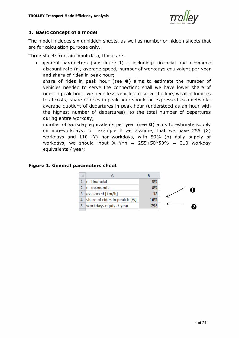
general parameters (see figure 1) – including: financial and economic
discount rate (r), average speed, number of workdays equivalent per year
and share of rides in peak hour;
share of rides in peak hour (see ) aims to estimate the number of
vehicles needed to serve the connection; shall we have lower share of
rides in peak hour, we need less vehicles to serve the line, what influences
total costs; share of rides in peak hour should be expressed as a network-
average quotient of departures in peak hour (understood as an hour with
the highest number of departures), to the total number of departures
during entire workday;
number of workday equivalents per year (see ) aims to estimate supply
on non-workdays; for example if we assume, that we have 255 (X)
workdays and 110 (Y) non-workdays, with 50% (n) daily supply of
workdays, we should input X+Y*n = 255+50*50% = 310 workday
equivalents / year;
Figure 1. General parameters sheet
TROLLEY Transport Mode Efficiency Analysis
5 of 24
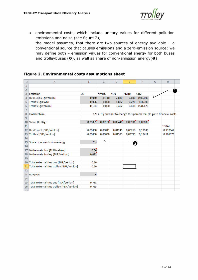
environmental costs, which include unitary values for different pollution
emissions and noise (see figure 2);
the model assumes, that there are two sources of energy available – a
conventional source that causes emissions and a zero-emission source; we
may define both – emission values for conventional energy for both buses
and trolleybuses (), as well as share of non-emission energy();
Figure 2. Environmental costs assumptions sheet
TROLLEY Transport Mode Efficiency Analysis
6 of 24
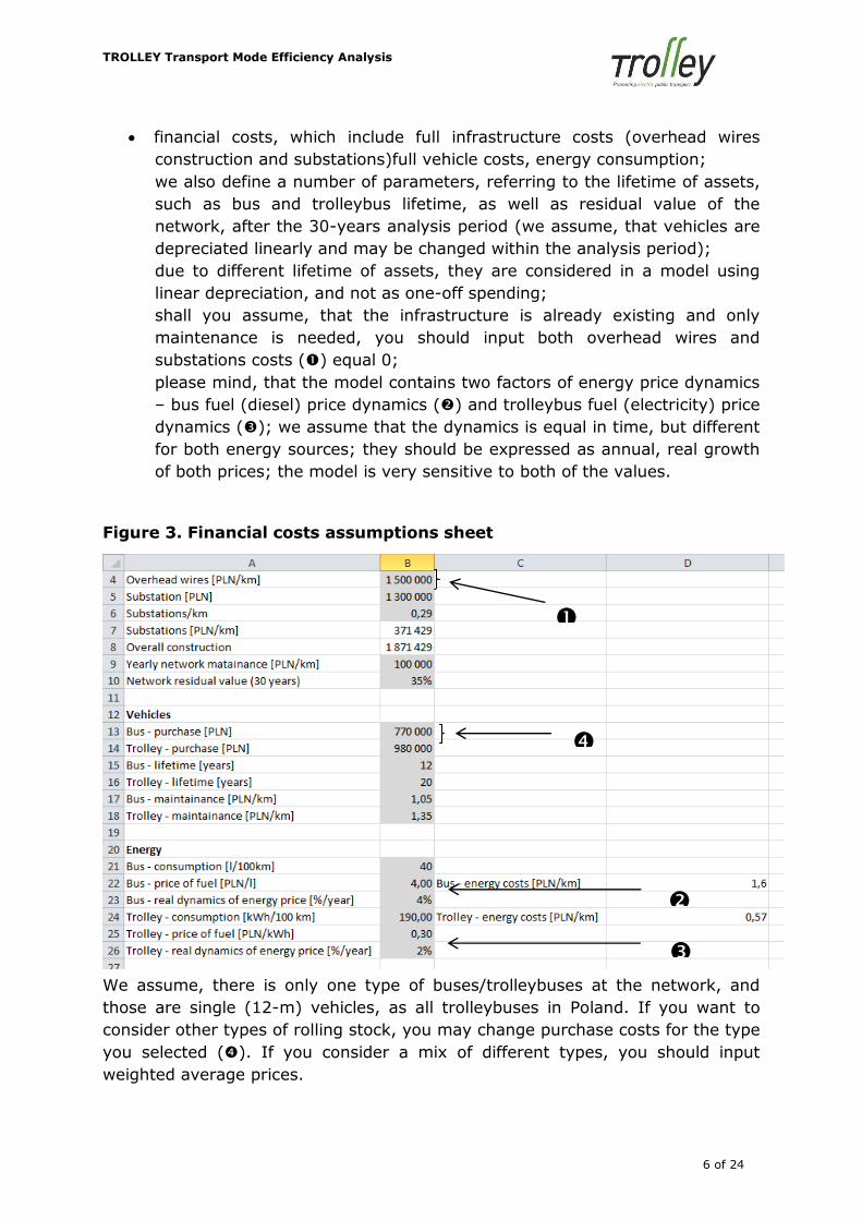
financial costs, which include full infrastructure costs (overhead wires
construction and substations)full vehicle costs, energy consumption;
we also define a number of parameters, referring to the lifetime of assets,
such as bus and trolleybus lifetime, as well as residual value of the
network, after the 30-years analysis period (we assume, that vehicles are
depreciated linearly and may be changed within the analysis period);
due to different lifetime of assets, they are considered in a model using
linear depreciation, and not as one-off spending;
shall you assume, that the infrastructure is already existing and only
maintenance is needed, you should input both overhead wires and
substations costs () equal 0;
please mind, that the model contains two factors of energy price dynamics
– bus fuel (diesel) price dynamics () and trolleybus fuel (electricity) price
dynamics (); we assume that the dynamics is equal in time, but different
for both energy sources; they should be expressed as annual, real growth
of both prices; the model is very sensitive to both of the values.
Figure 3. Financial costs assumptions sheet
We assume, there is only one type of buses/trolleybuses at the network, and
those are single (12-m) vehicles, as all trolleybuses in Poland. If you want to
consider other types of rolling stock, you may change purchase costs for the type
you selected (). If you consider a mix of different types, you should input
weighted average prices.
TROLLEY Transport Mode Efficiency Analysis
7 of 24
Please mind, that only grey cells should be edited and contain input
variables. White cells contain numbers derived from other values.
The three other sheets contain output data, presented on graphs for easier
interpretation. The graphs change automatically, every time we change our
assumptions, therefore it’s important to save entire Excel file for each set of
assumption, under a new file name.
Before passing to the output data, please mind, that the model omits some
costs, that are equal for bus and trolleybus transport, such as for example
personal costs. The model basically presents the data for 1 km of two-directions
trolleybus line, i.e. all costs are estimated for such section.
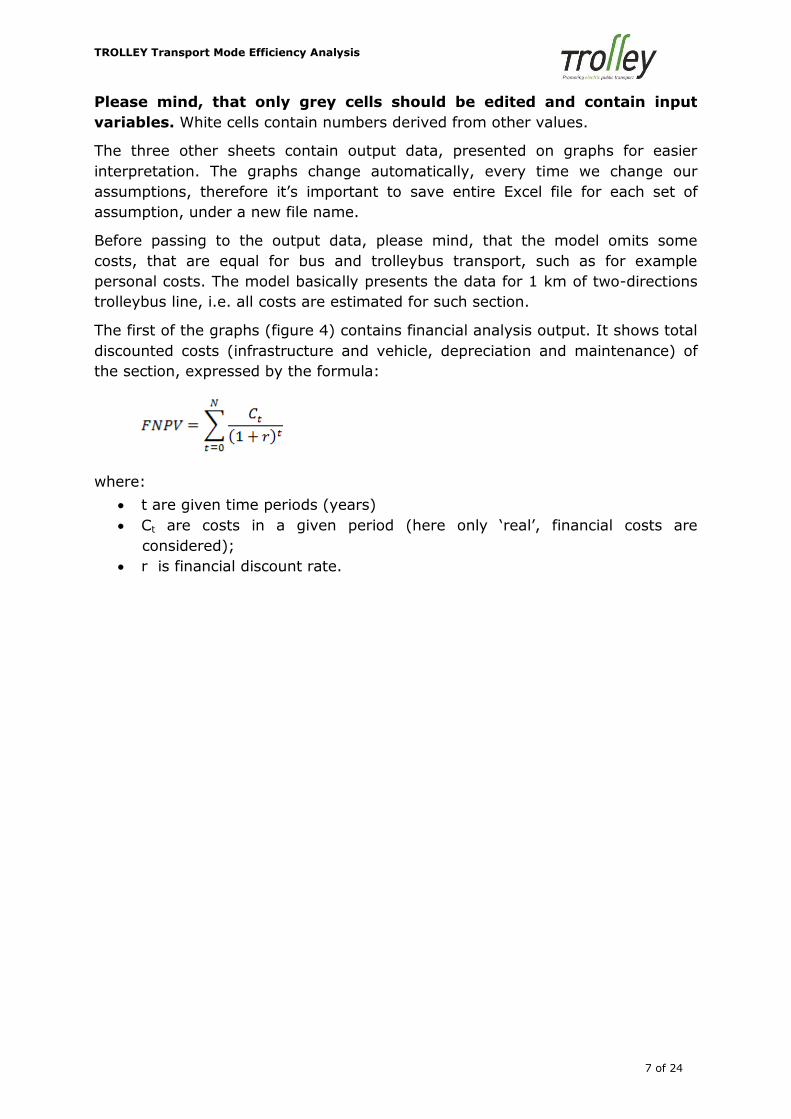
The first of the graphs (figure 4) contains financial analysis output. It shows total
discounted costs (infrastructure and vehicle, depreciation and maintenance) of
the section, expressed by the formula:
where:
t are given time periods (years)
Ct are costs in a given period (here only ‘real’, financial costs are
considered);
r is financial discount rate.
TROLLEY Transport Mode Efficiency Analysis
8 of 24
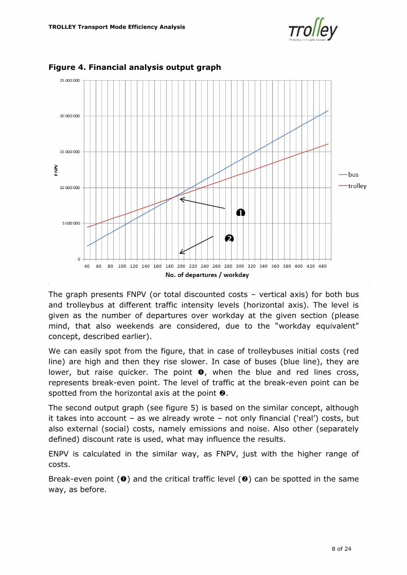
Figure 4. Financial analysis output graph
The graph presents FNPV (or total discounted costs – vertical axis) for both bus
and trolleybus at different traffic intensity levels (horizontal axis). The level is
given as the number of departures over workday at the given section (please
mind, that also weekends are considered, due to the “workday equivalent”
concept, described earlier).
We can easily spot from the figure, that in case of trolleybuses initial costs (red
line) are high and then they rise slower. In case of buses (blue line), they are
lower, but raise quicker. The point , when the blue and red lines cross,
represents break-even point. The level of traffic at the break-even point can be
spotted from the horizontal axis at the point .
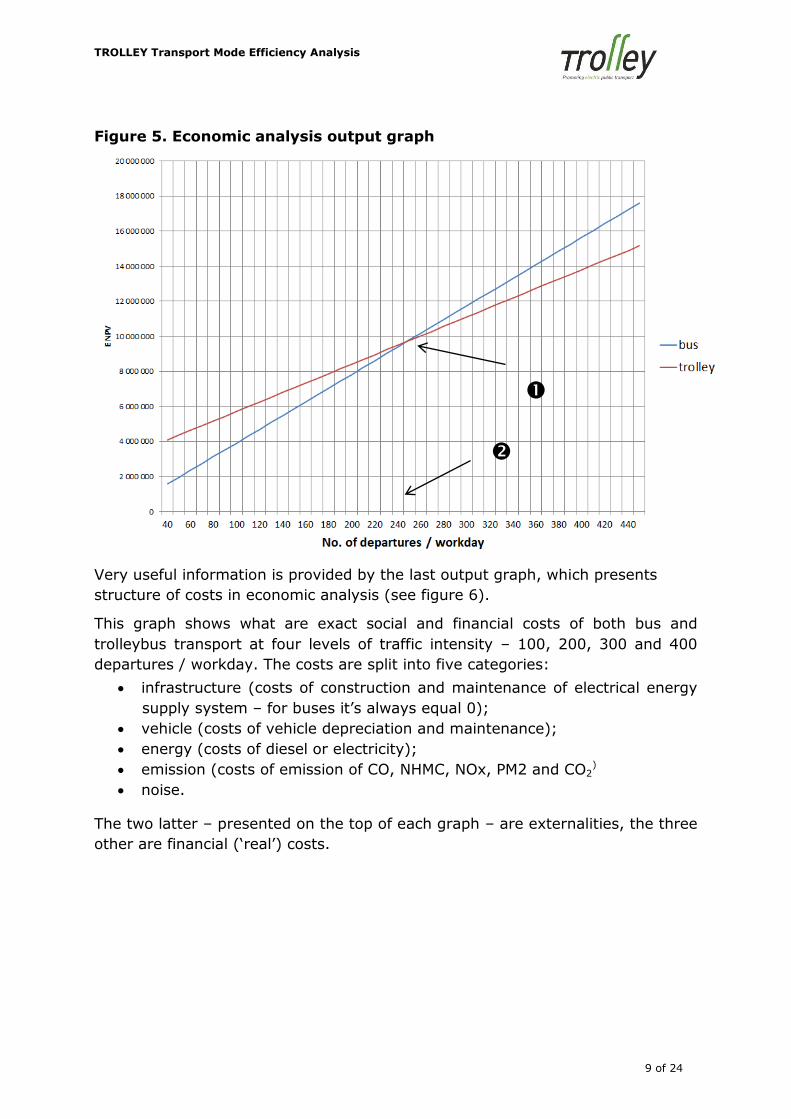
The second output graph (see figure 5) is based on the similar concept, although
it takes into account – as we already wrote – not only financial (‘real’) costs, but
also external (social) costs, namely emissions and noise. Also other (separately
defined) discount rate is used, what may influence the results.
ENPV is calculated in the similar way, as FNPV, just with the higher range of
costs.
Break-even point () and the critical traffic level () can be spotted in the same
way, as before.
TROLLEY Transport Mode Efficiency Analysis
9 of 24
Figure 5. Economic analysis output graph
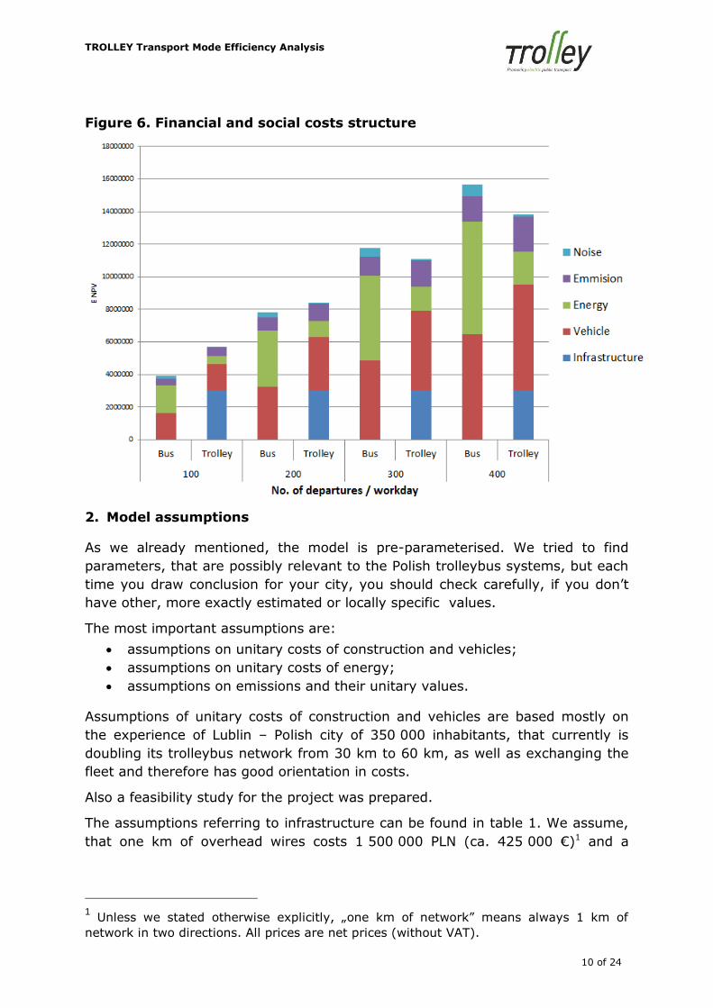
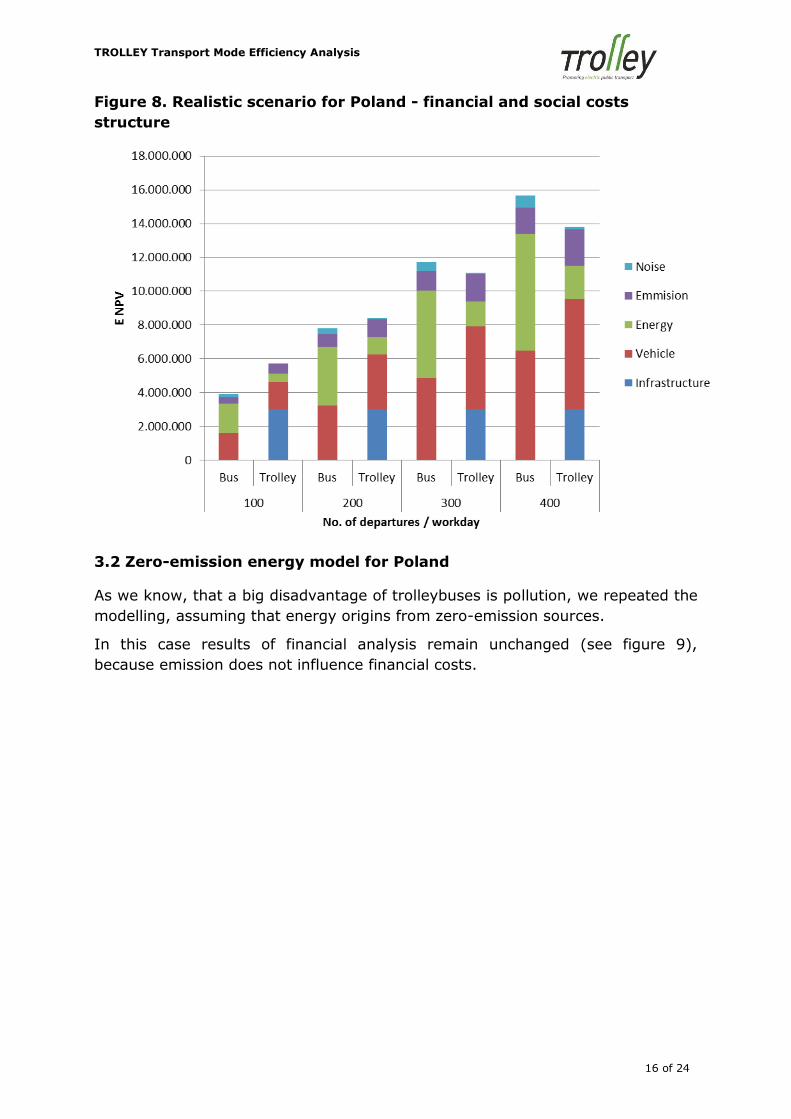
Very useful information is provided by the last output graph, which presents
structure of costs in economic analysis (see figure 6).
This graph shows what are exact social and financial costs of both bus and
trolleybus transport at four levels of traffic intensity – 100, 200, 300 and 400
departures / workday. The costs are split into five categories:
infrastructure (costs of construction and maintenance of electrical energy
supply system – for buses it’s always equal 0);
vehicle (costs of vehicle depreciation and maintenance);
energy (costs of diesel or electricity);
emission (costs of emission of CO, NHMC, NOx, PM2 and CO2)
noise.
The two latter – presented on the top of each graph – are externalities, the three
other are financial (‘real’) costs.
TROLLEY Transport Mode Efficiency Analysis
10 of 24
Figure 6. Financial and social costs structure
2. Model assumptions
As we already mentioned, the model is pre-parameterised. We tried to find
parameters, that are possibly relevant to the Polish trolleybus systems, but each
time you draw conclusion for your city, you should check carefully, if you don’t
have other, more exactly estimated or locally specific values.
The most important assumptions are:
assumptions on unitary costs of construction and vehicles;
assumptions on unitary costs of energy;
assumptions on emissions and their unitary values.
Assumptions of unitary costs of construction and vehicles are based mostly on
the experience of Lublin – Polish city of 350 000 inhabitants, that currently is
doubling its trolleybus network from 30 km to 60 km, as well as exchanging the
fleet and therefore has good orientation in costs.
Also a feasibility study for the project was prepared.
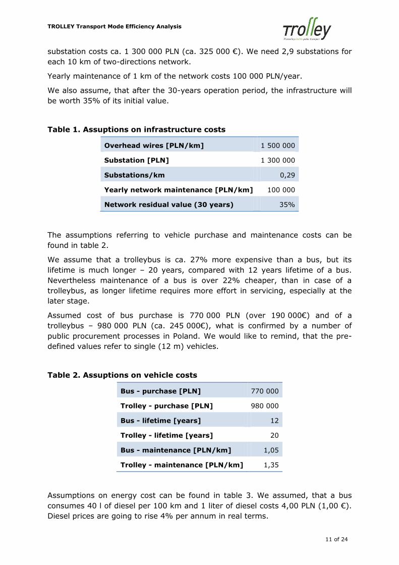
The assumptions referring to infrastructure can be found in table 1. We assume,
that one km of overhead wires costs 1 500 000 PLN (ca. 425 000 €)1 and a
1 Unless we stated otherwise explicitly, „one km of network” means always 1 km of
network in two directions. All prices are net prices (without VAT).
TROLLEY Transport Mode Efficiency Analysis
11 of 24
substation costs ca. 1 300 000 PLN (ca. 325 000 €). We need 2,9 substations for
each 10 km of two-directions network.
Yearly maintenance of 1 km of the network costs 100 000 PLN/year.
We also assume, that after the 30-years operation period, the infrastructure will
be worth 35% of its initial value.
Table 1. Assuptions on infrastructure costs
Overhead wires [PLN/km] 1 500 000
Substation [PLN] 1 300 000
Substations/km 0,29
Yearly network maintenance [PLN/km] 100 000
Network residual value (30 years) 35%
The assumptions referring to vehicle purchase and maintenance costs can be
found in table 2.
We assume that a trolleybus is ca. 27% more expensive than a bus, but its
lifetime is much longer – 20 years, compared with 12 years lifetime of a bus.
Nevertheless maintenance of a bus is over 22% cheaper, than in case of a
trolleybus, as longer lifetime requires more effort in servicing, especially at the
later stage.
Assumed cost of bus purchase is 770 000 PLN (over 190 000€) and of a
trolleybus – 980 000 PLN (ca. 245 000€), what is confirmed by a number of
public procurement processes in Poland. We would like to remind, that the pre-
defined values refer to single (12 m) vehicles.
Table 2. Assuptions on vehicle costs
Bus - purchase [PLN] 770 000
Trolley - purchase [PLN] 980 000
Bus - lifetime [years] 12
Trolley - lifetime [years] 20
Bus - maintenance [PLN/km] 1,05
Trolley - maintenance [PLN/km] 1,35
Assumptions on energy cost can be found in table 3. We assumed, that a bus
consumes 40 l of diesel per 100 km and 1 liter of diesel costs 4,00 PLN (1,00 €).
Diesel prices are going to rise 4% per annum in real terms.
TROLLEY Transport Mode Efficiency Analysis
12 of 24
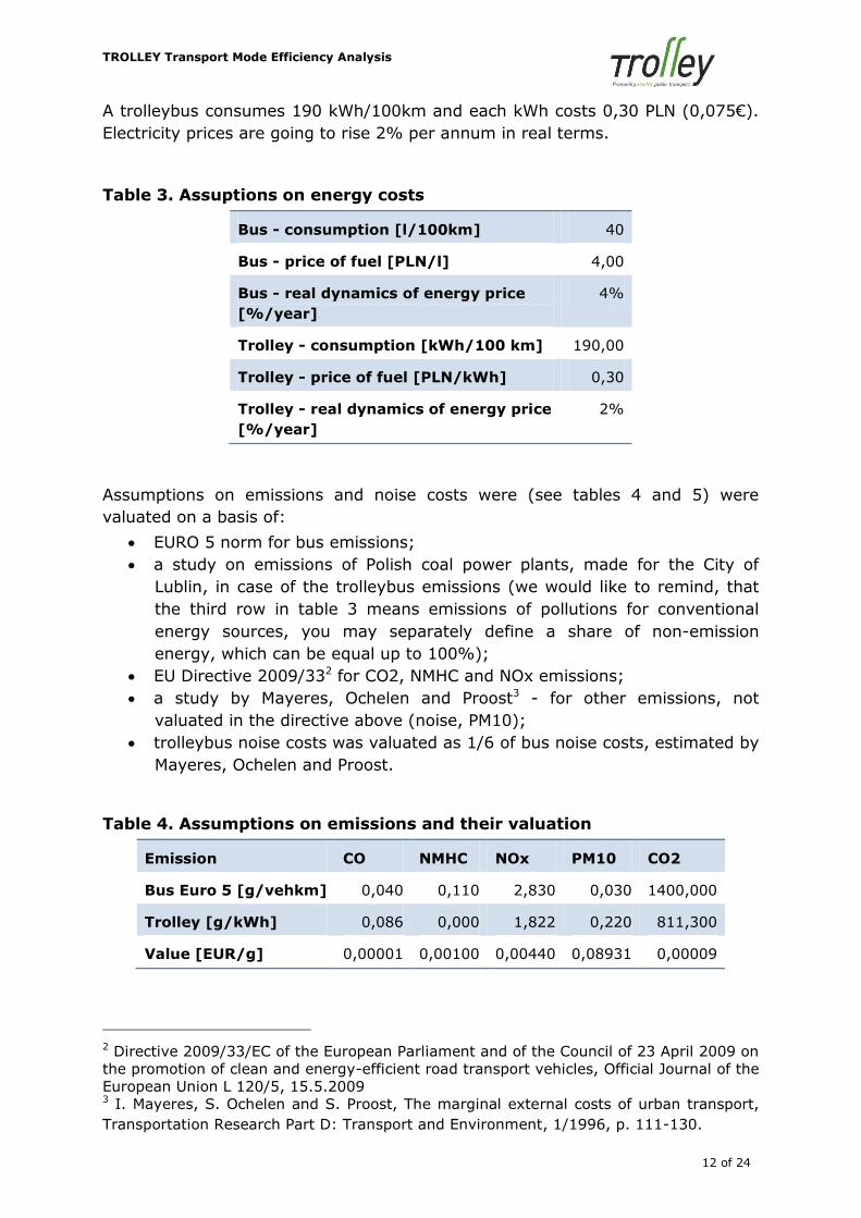
A trolleybus consumes 190 kWh/100km and each kWh costs 0,30 PLN (0,075€).
Electricity prices are going to rise 2% per annum in real terms.
Table 3. Assuptions on energy costs
Bus - consumption [l/100km] 40
Bus - price of fuel [PLN/l] 4,00
Bus - real dynamics of energy price
[%/year]
4%
Trolley - consumption [kWh/100 km] 190,00
Trolley - price of fuel [PLN/kWh] 0,30
Trolley - real dynamics of energy price
[%/year]
2%
Assumptions on emissions and noise costs were (see tables 4 and 5) were
valuated on a basis of:
EURO 5 norm for bus emissions;
a study on emissions of Polish coal power plants, made for the City of
Lublin, in case of the trolleybus emissions (we would like to remind, that
the third row in table 3 means emissions of pollutions for conventional
energy sources, you may separately define a share of non-emission
energy, which can be equal up to 100%);
EU Directive 2009/332 for CO2, NMHC and NOx emissions;
a study by Mayeres, Ochelen and Proost3 - for other emissions, not
valuated in the directive above (noise, PM10);
trolleybus noise costs was valuated as 1/6 of bus noise costs, estimated by
Mayeres, Ochelen and Proost.
Table 4. Assumptions on emissions and their valuation
Emission CO NMHC NOx PM10 CO2
Bus Euro 5 [g/vehkm] 0,040 0,110 2,830 0,030 1400,000
Trolley [g/kWh] 0,086 0,000 1,822 0,220 811,300
Value [EUR/g] 0,00001 0,00100 0,00440 0,08931 0,00009
2 Directive 2009/33/EC of the European Parliament and of the Council of 23 April 2009 on
the promotion of clean and energy-efficient road transport vehicles, Official Journal of the
European Union L 120/5, 15.5.2009 3 I. Mayeres, S. Ochelen and S. Proost, The marginal external costs of urban transport,
Transportation Research Part D: Transport and Environment, 1/1996, p. 111-130.
TROLLEY Transport Mode Efficiency Analysis
13 of 24
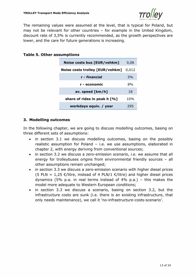
The remaining values were assumed at the level, that is typical for Poland, but
may not be relevant for other countries – for example in the United Kingdom,
discount rate of 3,5% is currently recommended, as the growth perspectives are
lower, and the care for future generations is increasing.
Table 5. Other assumptions
Noise costs bus [EUR/vehkm] 0,06
Noise costs trolley [EUR/vehkm] 0,012
r - financial 5%
r - economic 8%
av. speed [km/h] 18
share of rides in peak h [%] 10%
workdays equiv. / year 295
3. Modelling outcomes
In the following chapter, we are going to discuss modelling outcomes, basing on
three different sets of assumptions:
in section 3.1 we discuss modelling outcomes, basing on the possibly
realistic assumption for Poland – i.e. we use assumptions, elaborated in
chapter 2, with energy deriving from conventional sources;
in section 3.2 we discuss a zero-emission scenario, i.e. we assume that all
energy for trolleybuses origins from environmental friendly sources – all
other assumptions remain unchanged;
in section 3.3 we discuss a zero-emission scenario with higher diesel prices
(5 PLN = 1,25 €/litre, instead of 4 PLN/1 €/litre) and higher diesel prices
dynamics (5% p.a. in real terms instead of 4% p.a.) – this makes the
model more adequate to Western European conditions;
in section 3.3 we discuss a scenario, basing on section 3.2, but the
infrastructure costs are sunk (i.e. there is an existing infrastructure, that
only needs maintenance), we call it ‘no-infrastructure-costs-scenario’.
TROLLEY Transport Mode Efficiency Analysis
14 of 24
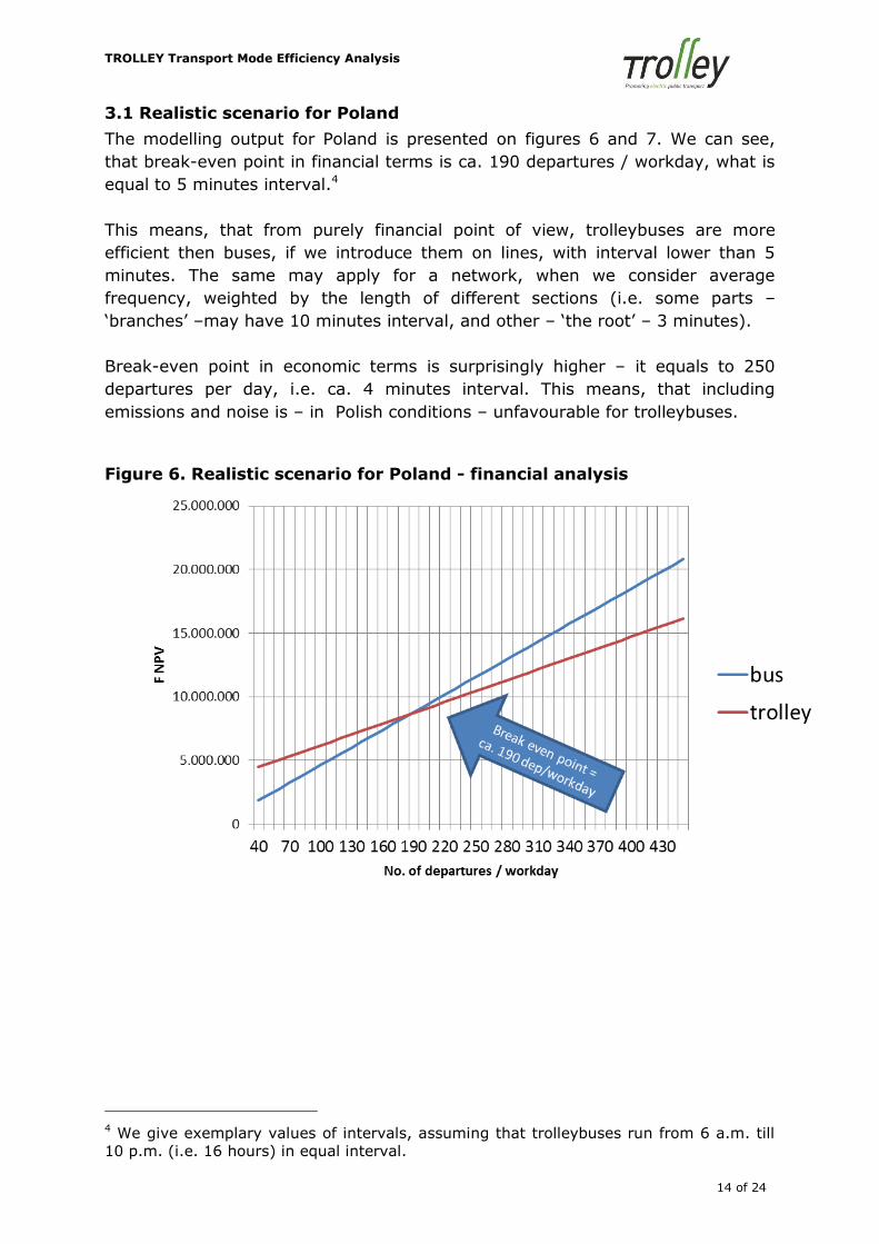
3.1 Realistic scenario for Poland
The modelling output for Poland is presented on figures 6 and 7. We can see,
that break-even point in financial terms is ca. 190 departures / workday, what is
equal to 5 minutes interval.4
This means, that from purely financial point of view, trolleybuses are more
efficient then buses, if we introduce them on lines, with interval lower than 5
minutes. The same may apply for a network, when we consider average
frequency, weighted by the length of different sections (i.e. some parts –
‘branches’ –may have 10 minutes interval, and other – ‘the root’ – 3 minutes).
Break-even point in economic terms is surprisingly higher – it equals to 250
departures per day, i.e. ca. 4 minutes interval. This means, that including
emissions and noise is – in Polish conditions – unfavourable for trolleybuses.
Figure 6. Realistic scenario for Poland - financial analysis
4 We give exemplary values of intervals, assuming that trolleybuses run from 6 a.m. till
10 p.m. (i.e. 16 hours) in equal interval.
TROLLEY Transport Mode Efficiency Analysis
15 of 24
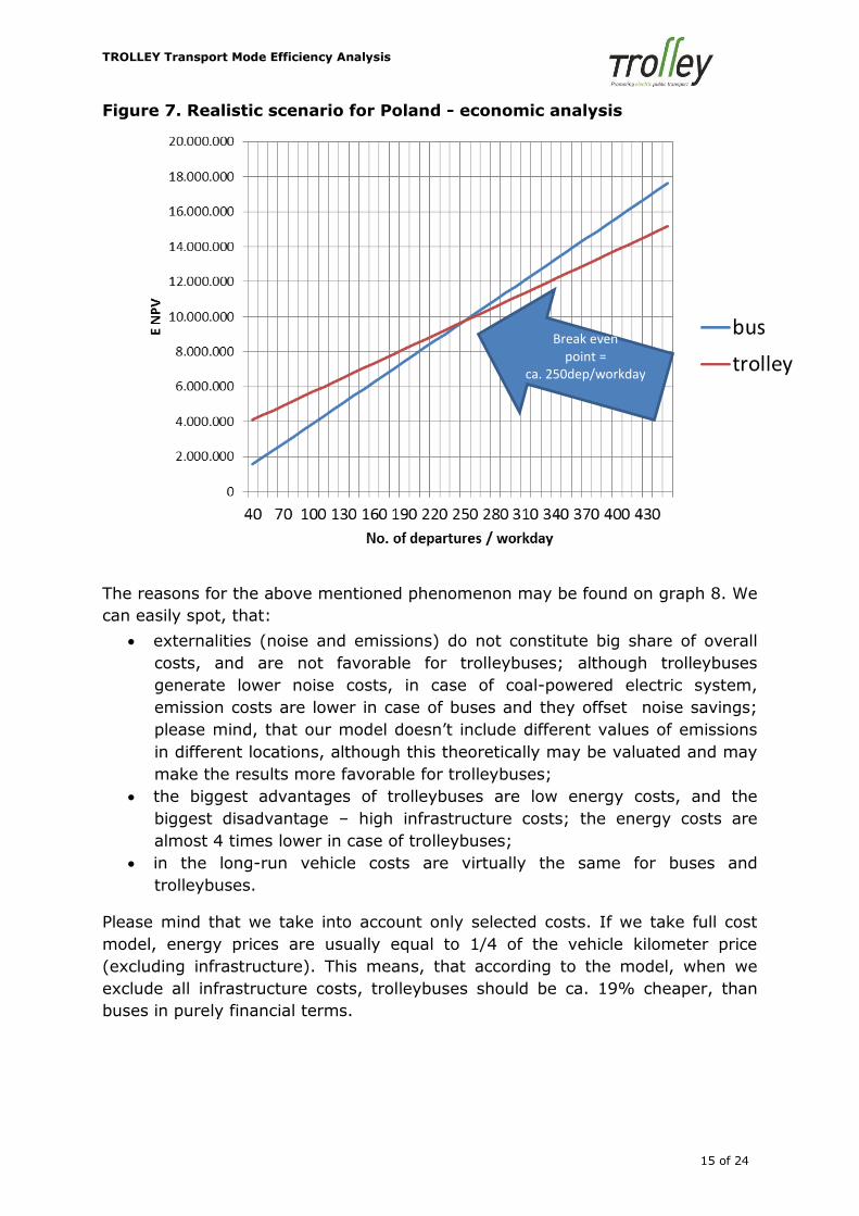
Figure 7. Realistic scenario for Poland - economic analysis
The reasons for the above mentioned phenomenon may be found on graph 8. We
can easily spot, that:
externalities (noise and emissions) do not constitute big share of overall
costs, and are not favorable for trolleybuses; although trolleybuses
generate lower noise costs, in case of coal-powered electric system,
emission costs are lower in case of buses and they offset noise savings;
please mind, that our model doesn’t include different values of emissions
in different locations, although this theoretically may be valuated and may
make the results more favorable for trolleybuses;
the biggest advantages of trolleybuses are low energy costs, and the
biggest disadvantage – high infrastructure costs; the energy costs are
almost 4 times lower in case of trolleybuses;
in the long-run vehicle costs are virtually the same for buses and
trolleybuses.
Please mind that we take into account only selected costs. If we take full cost
model, energy prices are usually equal to 1/4 of the vehicle kilometer price
(excluding infrastructure). This means, that according to the model, when we
exclude all infrastructure costs, trolleybuses should be ca. 19% cheaper, than
buses in purely financial terms.
Break even point =
ca. 250dep/workday
TROLLEY Transport Mode Efficiency Analysis
16 of 24
Figure 8. Realistic scenario for Poland - financial and social costs
structure
3.2 Zero-emission energy model for Poland
As we know, that a big disadvantage of trolleybuses is pollution, we repeated the
modelling, assuming that energy origins from zero-emission sources.
In this case results of financial analysis remain unchanged (see figure 9),
because emission does not influence financial costs.
TROLLEY Transport Mode Efficiency Analysis
17 of 24
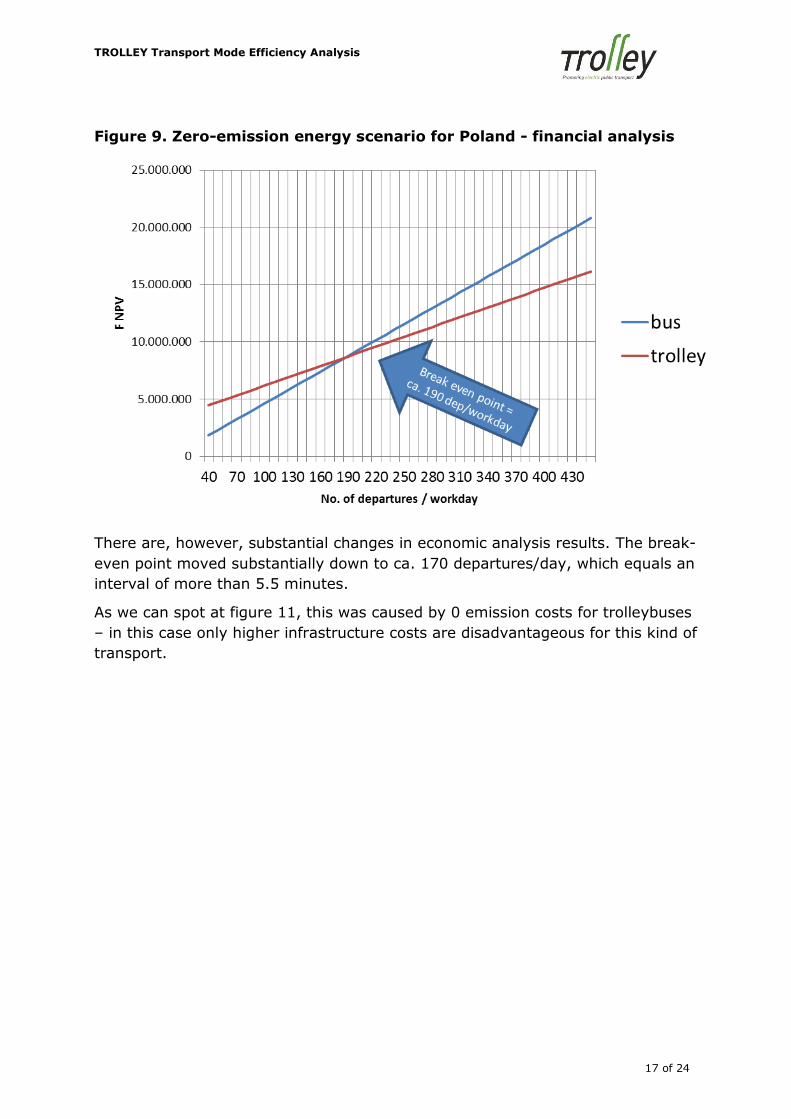
Figure 9. Zero-emission energy scenario for Poland - financial analysis
There are, however, substantial changes in economic analysis results. The break-
even point moved substantially down to ca. 170 departures/day, which equals an
interval of more than 5.5 minutes.
As we can spot at figure 11, this was caused by 0 emission costs for trolleybuses
– in this case only higher infrastructure costs are disadvantageous for this kind of
transport.
TROLLEY Transport Mode Efficiency Analysis
18 of 24
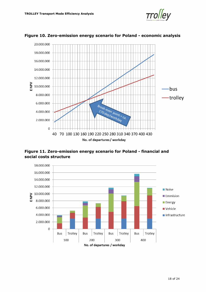
Figure 10. Zero-emission energy scenario for Poland - economic analysis
Figure 11. Zero-emission energy scenario for Poland - financial and
social costs structure
TROLLEY Transport Mode Efficiency Analysis
19 of 24
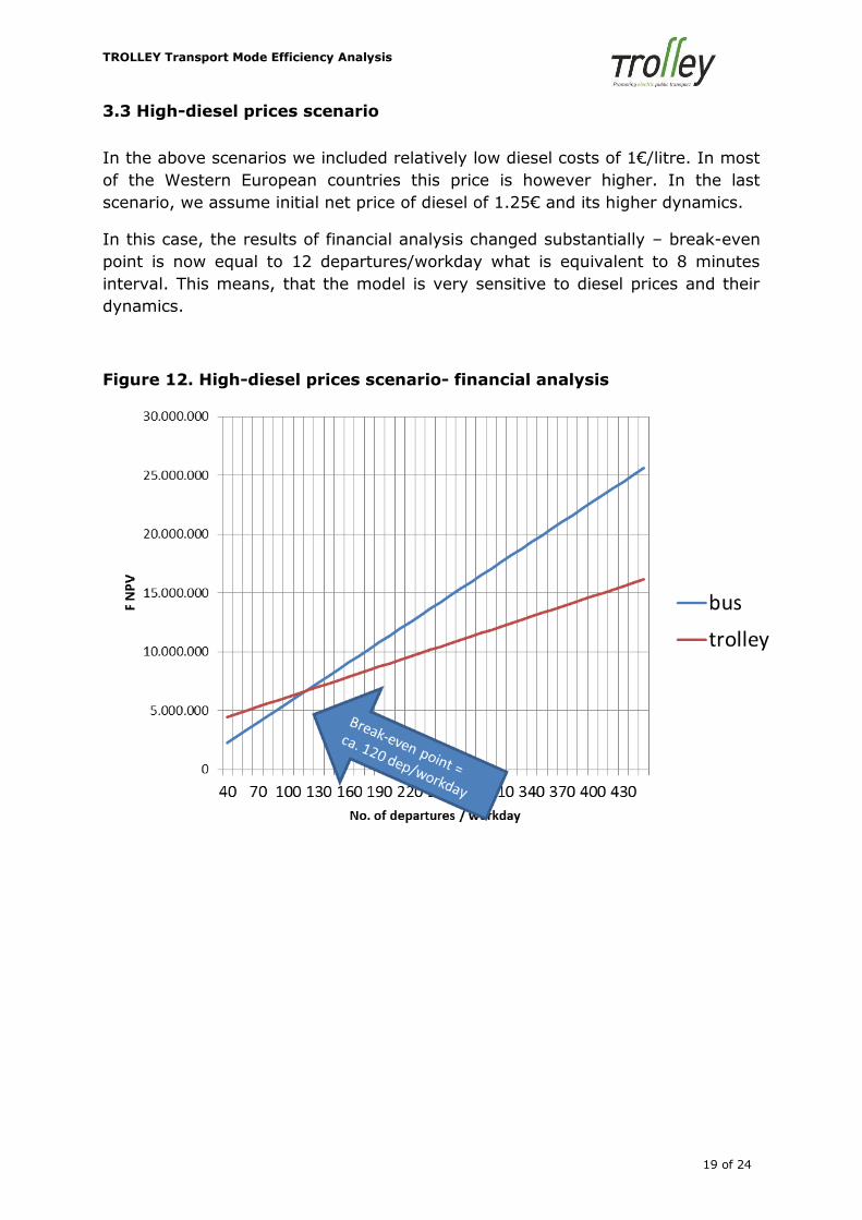
3.3 High-diesel prices scenario
In the above scenarios we included relatively low diesel costs of 1€/litre. In most
of the Western European countries this price is however higher. In the last
scenario, we assume initial net price of diesel of 1.25€ and its higher dynamics.
In this case, the results of financial analysis changed substantially – break-even
point is now equal to 12 departures/workday what is equivalent to 8 minutes
interval. This means, that the model is very sensitive to diesel prices and their
dynamics.
Figure 12. High-diesel prices scenario- financial analysis
TROLLEY Transport Mode Efficiency Analysis
20 of 24
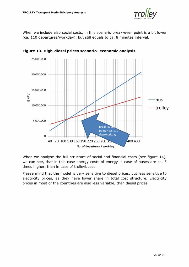
When we include also social costs, in this scenario break-even point is a bit lower
(ca. 110 departures/workday), but still equals to ca. 8 minutes interval.
Figure 13. High-diesel prices scenario- economic analysis
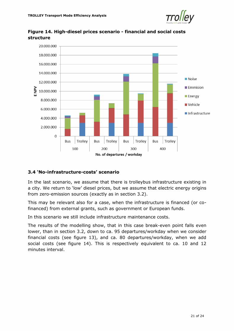
When we analyse the full structure of social and financial costs (see figure 14),
we can see, that in this case energy costs of energy in case of buses are ca. 5
times higher, than in case of trolleybuses.
Please mind that the model is very sensitive to diesel prices, but less sensitive to
electricity prices, as they have lower share in total cost structure. Electricity
prices in most of the countries are also less variable, than diesel prices.
Break-even point = ca. 110 dep/workday
TROLLEY Transport Mode Efficiency Analysis
21 of 24
Figure 14. High-diesel prices scenario - financial and social costs
structure
3.4 ‘No-infrastructure-costs’ scenario
In the last scenario, we assume that there is trolleybus infrastructure existing in
a city. We return to ‘low’ diesel prices, but we assume that electric energy origins
from zero-emission sources (exactly as in section 3.2).
This may be relevant also for a case, when the infrastructure is financed (or co-
financed) from external grants, such as government or European funds.
In this scenario we still include infrastructure maintenance costs.
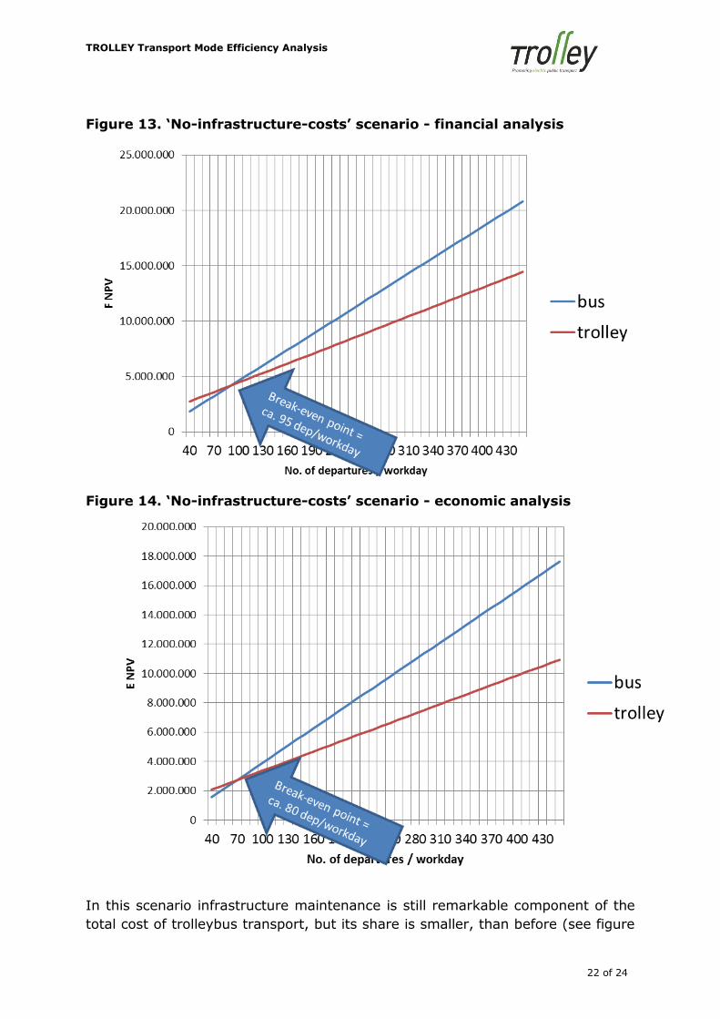
The results of the modelling show, that in this case break-even point falls even
lower, than in section 3.2, down to ca. 95 departures/workday when we consider
financial costs (see figure 13), and ca. 80 departures/workday, when we add
social costs (see figure 14). This is respectively equivalent to ca. 10 and 12
minutes interval.
TROLLEY Transport Mode Efficiency Analysis
22 of 24
Figure 13. ‘No-infrastructure-costs’ scenario - financial analysis
Figure 14. ‘No-infrastructure-costs’ scenario - economic analysis
In this scenario infrastructure maintenance is still remarkable component of the
total cost of trolleybus transport, but its share is smaller, than before (see figure
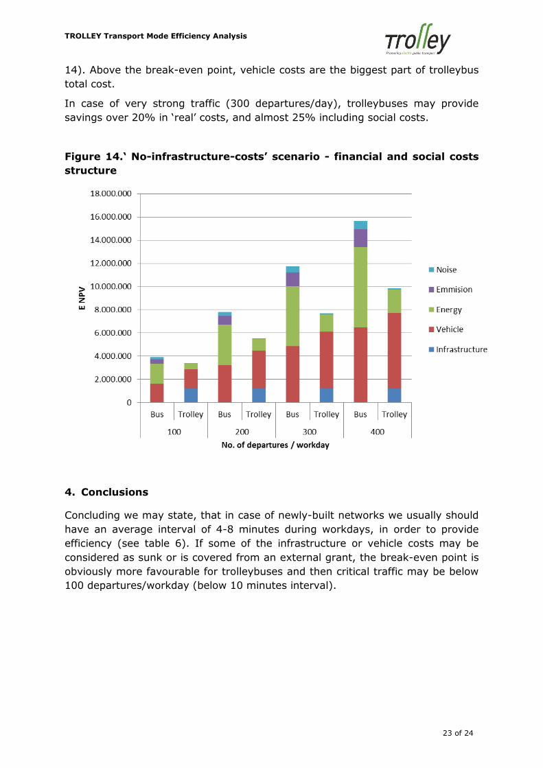
TROLLEY Transport Mode Efficiency Analysis
23 of 24
14). Above the break-even point, vehicle costs are the biggest part of trolleybus
total cost.
In case of very strong traffic (300 departures/day), trolleybuses may provide
savings over 20% in ‘real’ costs, and almost 25% including social costs.
Figure 14.‘ No-infrastructure-costs’ scenario - financial and social costs
structure
4. Conclusions
Concluding we may state, that in case of newly-built networks we usually should
have an average interval of 4-8 minutes during workdays, in order to provide
efficiency (see table 6). If some of the infrastructure or vehicle costs may be
considered as sunk or is covered from an external grant, the break-even point is
obviously more favourable for trolleybuses and then critical traffic may be below
100 departures/workday (below 10 minutes interval).
TROLLEY Transport Mode Efficiency Analysis
24 of 24
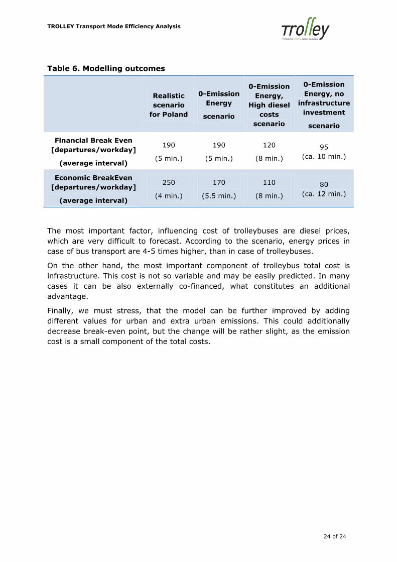
Table 6. Modelling outcomes
Realistic
scenario
for Poland
0-Emission
Energy
scenario
0-Emission
Energy,
High diesel
costs
scenario
0-Emission
Energy, no
infrastructure
investment
scenario
Financial Break Even
[departures/workday]
(average interval)
190
(5 min.)
190
(5 min.)
120
(8 min.)
95
(ca. 10 min.)
Economic BreakEven
[departures/workday]
(average interval)
250
(4 min.)
170
(5.5 min.)
110
(8 min.)
80
(ca. 12 min.)
The most important factor, influencing cost of trolleybuses are diesel prices,
which are very difficult to forecast. According to the scenario, energy prices in
case of bus transport are 4-5 times higher, than in case of trolleybuses.
On the other hand, the most important component of trolleybus total cost is
infrastructure. This cost is not so variable and may be easily predicted. In many
cases it can be also externally co-financed, what constitutes an additional
advantage.
Finally, we must stress, that the model can be further improved by adding
different values for urban and extra urban emissions. This could additionally
decrease break-even point, but the change will be rather slight, as the emission
cost is a small component of the total costs.


![Lecture 5 Transport [Compatibility Mode]](https://img.pdfslide.us/doc/110x75/577dab1f1a28ab223f8bf81c/lecture-5-transport-compatibility-mode.jpg)
![cell membrane transport [Compatibility Mode]](https://img.pdfslide.us/doc/110x75/577d2ba81a28ab4e1eab060d/cell-membrane-transport-compatibility-mode.jpg)