TripleBit: a Fast and Compact System for Large Scale RDFData

Pingpeng Yuan, Pu Liu, Buwen Wu,Hai Jin, Wenya Zhang

Services Computing Tech. and System Lab.School of Computer Science & Technology

Huazhong University of Science and Technology,China

ppyuan, hjin@hust.edu.cn

Ling LiuDistributed Data Intensive Systems Lab.

School of Computer ScienceCollege of Computing

Georgia Institute of Technology, USA

lingliu@cc.gatech.edu

ABSTRACTThe volume of RDF data continues to grow over the past decadeand many known RDF datasets have billions of triples. A grantchallenge of managing this huge RDF data is how to access thisbig RDF data efficiently. A popular approach to addressing theproblem is to build a full set of permutations of (S, P, O) index-es. Although this approach has shown to accelerate joins by order-s of magnitude, the large space overhead limits the scalability ofthis approach and makes it heavyweight. In this paper, we presentTripleBit, a fast and compact system for storing and accessing RDFdata. The design of TripleBit has three salient features. First, thecompact design of TripleBit reduces both the size of stored RDFdata and the size of its indexes. Second, TripleBit introduces twoauxiliary index structures, ID-Chunk bit matrix and ID-Predicatebit matrix, to minimize the cost of index selection during queryevaluation. Third, its query processor dynamically generates anoptimal execution ordering for join queries, leading to fast queryexecution and effective reduction on the size of intermediate re-sults. Our experiments show that TripleBit outperforms RDF-3X,MonetDB, BitMat on LUBM, UniProt and BTC 2012 benchmarkqueries and it offers orders of mangnitude performance improve-ment for some complex join queries.

1. INTRODUCTIONThe Resource Description Framework (RDF) data model and its

query language SPARQL are widely adopted today for managingschema-free structured information. Large amount of semantic dataare available in the RDF format in many fields of science, engineer-ing, and business, including bioinformatics, life sciences, businessintelligence and social networks. A growing number of organiza-tions or Community driven projects, such as White House, NewYork Times, Wikipedia and Science Commons, have begun export-ing RDF data [22]. Linked Open Data Project announced 52 billiontriples were published by March 2012 [22].

RDF data are a collection of triples, each with three columns,denoted by Subject (S), Predicate (P) and Object (O). RDF triples

Permission to make digital or hard copies of all or part of this work forpersonal or classroom use is granted without fee provided that copies arenot made or distributed for profit or commercial advantage and that copiesbear this notice and the full citation on the first page. To copy otherwise, torepublish, to post on servers or to redistribute to lists, requires prior specificpermission and/or a fee. Articles from this volume were invited to presenttheir results at The 39th International Conference on Very Large Data Bases,August 26th - 30th 2013, Riva del Garda, Trento, Italy.Proceedings of the VLDB Endowment, Vol. 6, No. 7Copyright 2013 VLDB Endowment 2150-8097/13/05... $ 10.00.

tend to have rich relationships, forming a huge and complex RD-F graph. Managing large-scale RDF data imposes technical chal-lenges to the conventional storage layout, indexing and query pro-cessing [17, 18]. A fair amount of work has been engaged in RDFdata management. Triples table [8, 17], column store with verti-cally partitioning [3] and property tables [25] are the three mostpopular alternative storage layouts for storing and accessing RD-F data. The storage layouts may not favor all queries. However,queries constrained on S, P or O values are equally important forreal-world applications. A popular approach to achieving this goalis to maintain all six permutation indexes on the RDF data in orderto provide efficient query processing for all possible access pat-terns [5, 9, 17, 24]. Although the permutation indexing techniquescan speed up joins by orders of magnitude, they may result in sig-nificant demand for both main memory and disk storage. First,RDF stores need load those indexes into limited memory of com-puter in order to generate query plans when processing complexjoin queries. Consequently, frequent memory swap in/out, and outof memory problems are common when querying RDF data withover a billion of triples [14]. Furthermore, the large space overheadalso places a heavy burden on both memory and disk I/O. One wayto address the space cost is to use compression techniques, such asD-Gap [5], delta compression [17], in storing and accessing RDFdata. Multiple permutation indexes also complicate the decision onthe choices of the indexes for a given query.

In this paper, we present TripleBit, a fast and compact systemfor large scale RDF data. TripeBit is designed based on two im-portant observations. First, it is important to design an RDF datastorage structure that can directly and efficiently query the com-pressed data. This motivates us to design a compact storage and in-dex structure in TripleBit. Second, in order to truly scale the RDFquery processor, we need efficient index structures and query eval-uation algorithms to minimize the size of intermediate results gen-erated when evaluating queries, especially complex join queries.This leads us to the design decision that we should not only reducethe size of indexes (e.g., through compression techniques) but alsominimize the number of indexes used in query evaluation.

The main contributions of the paper are three folds: First, wepresent a compact RDF store - TripleBit, including the design ofa bit matrix storage structure and the encoding-based compressionmethod for storing huge RDF graphs more efficiently. The stor-age structure enables TripleBit to use merge joins extensively forjoin processing. Second, we develop two auxiliary indexing struc-tures, ID-Chunk bit matrix and ID-Predicate bit matrix, to reducethe number and the size of indexes to the minimum while provid-ing orders of magnitude speedup for scan and merge-join perfor-

517

mance. The ID-Chunk bit matrix provides a fast search of the rel-evant chunks matching to a given subject (S) or object (O). TheID-Predicate bit matrix provides a mapping of a subject (S) or anobject (O) to the list of predicates to which it relates. Third, we em-ploy the dynamic query plan generation algorithm to generate anoptimal execution plan for a join query, aiming at reducing the sizeof intermediate results as early as possible. We evaluate TripleBitthrough extensive experiments against RDF graphs of up to 2.9 bil-lion triples. Our experimental comparison with the state of art RDFstores, such as RDF-3X, MonetDB, shows that the TripleBit consis-tently outperforms them and delivers up to 2-4 orders of magnitudebetter performance for complex long join queries over large scaleRDF data.

2. OVERVIEW & RELATED WORKA fair number of RDF storage systems has been developed in

the past decade, such as Sesame [8], Jena [25], RDF-3X [17, 18],Hexastore [24], BitMat [5], gStore [28] etc. These systems can bebroadly classified into four categories: triples table [17], proper-ty table [25], column store with vertical partitioning [3] and RDFgraph based store. We will illustrate and analyze these four cate-gories of RDF stores using the following example RDF dataset.

T1: person1 isNamed ”Tom”.T2: publication1 hasAuthor person1.T3: publication1 isTitled ”Pub1”.T4: person2 isNamed ”James”.T5: publication2 hasAuthor person2.T6: publication2 isTitled ”Pub2”.T7: publication1 hasCitation publication2.

Triple table. A natural approach to storing RDF data is to store(S, P, O) statements in a 3-column table with each row representinga RDF statement. The 3-column table is called the triple table [17].For the above example, the seven statements will correspond toseven rows of a triple table. There are several variants of the tripletable, e.g., storing literals and URIs in a separate table and usingpointers to refer to literals and URIs in the triple table. However,querying over an RDF table of billions of rows can be challenging.First, most of queries involve self-joins over this long table. Sec-ond, larger table size leads to larger table scan and larger index lookup time, which complicates both selectivity estimation and queryoptimization [3]. A popular approach to improving performance ofqueries over a triple table is to use an exhaustive indexing methodthat creates a full set of (S, P, O) permutations of indexes [17, 27].For example, RDF-3X, one of the best RDF stores today, built clus-tered B+-trees on all six (S, P, O) permutations− (SPO, SOP, PSO,POS, OSP, OPS), thus each RDF dataset is stored in six duplicates,one per index. In order to choose the fastest index among the sixindexes for a given query, another set of 9 aggregate indexes, in-cluding all six binary projections− (SP, SO, PO, PS, OS, OP), andthree unary projections − (S, P, O) [17, 18], are created and main-tained, each providing some selectivity statistics. By maintainingsuch aggregate indexes, RDF-3X eliminates the problem of expen-sive self-joins and provides significant performance improvement.However, storing all permutation indexes may be expensive and theperformance penalty can be high as the volume of dataset increasesdue to the cost of storing and accessing these indexes and the costof deciding which of these indexes to use at the query evaluation.Property table. Instead of using a ”long and slim” triple table, theproperty table typically stores RDF data in a ”fat” property tablewith subject as the first column and the list of distinct predicatesas the remaining columns [25]. Each row of the property tablecorresponds to a distinct S-value. Each of the remaining column-s corresponds to a predicate (P-value). Each table cell represents

an O-value of a triple with the given S-value and P-value. Con-sider our example RDF dataset of 7 triples with 4 distinct proper-ties (predicates), and thus we will have a 5-column property table.publication1 has three properties: hasAuthor, isTitled, hasCitation.Thus, three statements are mapped into one row corresponding topublication1 in the table. Clearly, for a big RDF dataset, a singleproperty table can be extremely sparse and contains many NUL-L values. Thus multiple-property tables with different clusters ofproperties are proposed in Jena [25] as an optimization technique.BitMat [5] represents an alternative design of the property tableapproach, in which RDF triples are represented as a 3D bit-cube,representing subjects, predicates and objects respectively and slic-ing along a dimension to get 2D matrices: SO, PO and PS.

An advantage of the property tables is that the subject-subjectself-joins on the subject column can be eliminated. However, theproperty table approach suffers from several problems [3]: First,the space overhead of the wide property table(s) with sparse at-tributes is high. Second, processing of RDF queries that have norestriction on property values may involve scanning all property ta-bles. Furthermore, experimental results in [12] have shown that theperformance of the property table approach degrades dramaticallywhen dealing with large scale RDF data.Column store with vertical partitioning. This approach storesRDF data [3] using multiple two-column tables, one for each u-nique predicate. The first column is for subject whereas the othercolumn is for object. Consider our running example with four prop-erties, this approach will map 7 statements to four 2-column tables.Although those tables can be stored using either row-oriented orcolumn-oriented DBMS, the column store is a more popular stor-age solution for vertically partitioned schema [3]. This approachis easy to implement and can provide superior performance forqueries with value-based restrictions on properties. However, thisapproach may suffer from scalability problems when the size of ta-bles varied significantly [19]. Furthermore, processing join querieswith multiple join conditions and unrestricted properties can be ex-tremely expensive due to the need of accessing all of the 2-columntables and the possibility of generating large intermediate results.Graph-based store. Graph-based approaches represent an orthog-onal dimension of RDF store research [7, 14], aiming at improvingthe performance of graph-based manipulations on RDF datasets be-yond RDF SPARQL queries. However, most of these graph basedapproaches focus more on improving the performance of special-ized graph operations rather than the scalability and efficiency ofRDF query processing [24]. Large scale RDF data is a very big s-parse graph, which poses a significant challenge to store and querysuch an RDF graph efficiently. [4] developed a compressed RD-F engine k2-triples. gStore [28] proposes VS-tree and VS*-treeindex to process both exact and wildcard SPARQL queries by effi-cient subgraph matching.

In comparison, TripleBit advocates two important design prin-ciples: First, in order to truly scale the RDF query processor, weshould design compact storage structure and minimize the num-ber of indexes used in query evaluation. Second, we need compactindex structure as well as efficient index utilization techniques tominimize the size of intermediate results generated during queryprocessing and to process complex joins efficiently.

3. TRIPLE MATRIX AND ITS STORAGESTRUCTURE

We design the TripleBit storage structure with three objectivesin mind: improving storage compactness, improving encoding orcompression efficiency and improving query processing efficiency.

518

Table 1: The Triple Matrix of the exampleisNamed hasAuthor isTitled hasCitationT1 T4 T2 T5 T3 T6 T7

person1 1 0 1 0 0 0 0person2 0 1 0 1 0 0 0publication1 0 0 1 0 1 0 1publication2 0 0 0 1 0 1 1”Tom” 1 0 0 0 0 0 0”James” 0 1 0 0 0 0 0”Pub1” 0 0 0 0 1 0 0”Pub2” 0 0 0 0 0 1 0

We first present the Triple Matrix model and then describe how thestorage layout design of the Triple Matrix model offers more com-pact storage, higher encoding efficiency and faster query execution.

In Triple Matrix model, RDF triples are represented as a two di-mensional bit matrix. We call it the triple matrix. Concretely, givenan RDF dataset, let VS , VP , VO and VT denote the set of distinctsubjects, predicates, objects and triples respectively, The triple ma-trix is created with entity e ∈ VE = VS ∪ VO as one dimension(row) and triples t ∈ VT as the other dimension (column). Thus,we can view the corresponding triple matrix as a two-dimensionaltable with |VT | columns and |VE | rows. Each column of the ma-trix corresponds to an RDF triple, with only two entries of bit value(’1’), corresponding to the subject entity and object entity of thetriple and all the rest of (|VE | − 2) entries of bit (’0’). Each rowis defined by a distinct entity value, with the presence (’1’) in asubset of entries, representing a collection of the triples having thesame entity. We sort the columns by predicates in lexicographicorder and vertically partition the matrix into multiple disjoint buck-ets, one per predicate (property). For a new triple with predicatep, it will be inserted into a column in the predicate bucket corre-sponding to p. Assume that the triple to be inserted has subject i,object j and predicate p, and it corresponds to the column k, thenthe entries that lie in the i-th row, the j-th row and the k-th columnof the matrix are set to ’1’. The other entries in the k-th column areset to ’0’. Table 1 shows the triple matrix for the running exampleof 7 triples. It has 7 columns, one per triple, and eight entities, rep-resenting four subject values and four object values. We use stringsinstead of row ids in this example solely for the readability.

In addition, during the construction of the triple matrix from RD-F data, each e ∈ VE is assigned a unique ID using the row numberin the matrix. We assign IDs to subjects and objects using the sameID space such that subjects and objects having identical values willbe treated as the same entity. We observe that a fair amount ofentities in many real RDF datasets are used as subject of a tripleand object of another triple. For example, Table 5 in Section 6showed that more than 57% subjects of UniProt are also object-s. TripleBit utilizes unique IDs for the same entities to achieve amore compact storage and to further improve the query process-ing efficiency. This is because query processor does not need todistinguish whether IDs represent subject or object entities whenprocessing joins. Furthermore, our approach facilitates index con-struction and makes the join on subject and object more efficientthan the approaches where subjects and objects have independentID space [5].

3.1 DictionaryIn RDF specification, Universal Resource Identifiers (URIs) are

used to identify resources, such as subjects and objects. A resourcemay have many properties and corresponding values. It is not e-conomical to store URIs in each appearance of resources. To re-duce the redundancy, like many RDF stores, such as RDF-3X, inTripleBit we replace all strings (URI, literals and blank node) by

Figure 1: String-ID Mapping and ID-String Mapping

IDs using mapping dictionaries. Considering the existence of longcommon prefixes in URIs, we adopt a prefix compression method,which is similar to Front Coding to obtain compressed dictionar-ies. The prefix compression method splits each URI into a prefixslice and a suffix slice at the last occurrence of separator ’/’. Thestrings which do not contain ’/’ are considered as suffixes. We as-sign each prefix a PrefixID and construct Prefix-ID mapping table.We concatenate prefix ID and suffix to get a new string which is al-so assigned an ID in an independent ID space. Similarly, we builda Suffix-ID mapping table (Fig. 1).

During query translation, hashing function maps prefix of a stringstr to its index and then the offset of prefix stored in correspondingslot of the hash table is accessed. Using the offset, we can get itsPrefixID in Prefix-ID mapping table. Using the above process, theID assigned to str is returned. The process to translate a string toits ID is illustrated using the solid lines in Fig. 1.

Before query results are returned to users or applications, IDs inthe results must be translated back into strings. In order to speed upthe reverse process, we build two inverted tables (PrefixID Offsetand ID Offset in Fig. 1) to translate IDs back into strings. Bothtables store (id, offset) pairs where id corresponds to the PrefixIDor IDs, and offset represents the position where the prefix or suffixand the ID are stored. Inverted table structures make the mappingof ids to literals or URIs more efficient. The process to transformids back to strings is shown by dashed line in Fig. 1.

In summary, searching ids in the dictionary using strings doesnot require much time thanks to the hashing index and the fact thatthe number of strings occurring in a query is very small. However,the reverse mapping process can be costly when the query resultsize is big [16].

3.2 ID Encoding in the Triple MatrixIn a triple matrix, ID is an integer. The size for storing an integer

is typically a word. Modern computers usually have a word size of32 bits or 64 bits. Not all integers require the whole word to storethem. For example, it is enough to store the ID of value ”100” using1 byte. It is wasteful to store values with a large number of byteswhen a small number of bytes are sufficient. Also, since TripleBitis designed for large scale RDF data, it is difficult to know the max-imal number of entities in future data sets. For example, 32-bits IDmight be a good choice for current RDF data, but insufficient in thenear future. Thus, we encode the entity ID in triple matrix usingvariable-size integer such that the minimum number of bytes areused to encode this integer. Furthermore, the most significant bit ofeach compressed byte is used to indicate whether an ID is the sub-ject(0) or object (1) of a statement and the remaining 7 bits are usedto store the value. Consider the example in Table 1. The entity per-

519

Figure 2: The Storage scheme of TripleBit

Table 2: Storage space of Triple Matrix for six datasetsLUBM

10MLUBM50M

LUBM100M

LUBM500M

LUBM1B UniProt

Two Copies of TripleMatrix (MB)

133 722 1,461 7,363 15,207 24,371

Per Triple (bytes) 5.02 5.48 5.54 5.59 5.97 4.33

son1 denotes a subject in T1 and an object in T2. Thus, the row ofthis entity has its 1st and 3rd columns set to ’1’. We use 00000001(subject) in the column encoding of T1 and use 10000001 (object)in the column encoding of T2 respectively. By utilizing the signif-icant bit of each compressed byte, we can easily find the triple ofinterest without scanning the entire chunk.

Many RDF stores use fixed-sized integer (e.g., an integer of 4bytes in 32-bit computer) to encode IDs. Comparing with fixed-sized integer, the overhead of the variable-size integer encodingapproach is 1 bit per byte but this approach saves more with high-er flexibility. Our experiments on the 6 datasets in Table 2 showthat each ID needs about 2.1-3 bytes on average. Furthermore, ourapproach is highly extensible comparing with fixed-sized ids sincethe former can encode any number of subjects or objects. For ex-ample, we can encode IDs larger than 232 using 5 or more byteswhile fixed-sized integer does not have such flexibility.

3.3 Triple Matrix Column CompressionThe triple matrix is inherently sparse. To achieve the internal

compact representation of the triple matrix, we store the bit ma-trix in a compressed format using column compression. Given thateach column of the matrix corresponds to a triple and thus hasonly two entries with ’1’, we show that a column-level compres-sion scheme for storing the triple matrix is more effective than therow-level, byte-level or bit-level compression scheme [5]. Con-cretely, for each column of the triple matrix, instead of storingthe entire column of size |VE |, we use only the two row numbers(i.e., IDs) that correspond to the two ’1’ entries. Consider Table1, the first column (T1) and the third column (T2) are represent-ed as 00000001 10000101 and 10000001 00000011 respectively.By combining with the variable-size integer encoding approach forthe two IDs, each column requires only 2-8 bytes for storing onetriple in TripleBit if the number of entities (or rows) is less than228. Furthermore, instead of storing two full ids of a column wecan store the first id and the changes between two ids. If two ids

are similar, it will further save storage. Our experiments on the sixdata sets in Table 2 show that the storage per triple is about 4.3-6bytes on average without other storage optimization. This saving atper-triple level is significant compared to 12 bytes per triple in therow stores and 8 bytes per triple in the column stores, leading tohigher efficiency in storing and scanning data on storage media aswell as high reduction in both the size of intermediate results andthe time complexity of query processing.

3.4 Triple Matrix Chunk StorageAs described earlier, we partition a triple matrix vertically in-

to predicate-based buckets, each containing triples with the samepredicate. Triples of each bucket are stored in fixed-size chunks.Chunks are physically clustered by predicates such that chunk clus-ters having the same predicates are placed adjacently on storagemedia. We assign chunks of each bucket with chunk IDs consec-utively. The size of a chunk can be set according to a number ofparameters, such as the size of dataset, the memory capacity, theIO page size. Although search in small size chunk is faster, largerchunk simplifies the construction of ID-Chunk index and reducesI/O. Larger chunk also has less storage overhead. In the first imple-mentation of TripleBit, we set the chunk size to be 64KB.

Since the triple matrix does not indicate which entity is subjector object in a column, we choose to store each column of a buck-et in a consistent order, either SO or OS. Compared to some ex-isting RDF systems [17, 24], which store all six permutations ofRDF data, TripleBit stores the triple matrix for each RDF datasetphysically in two duplicates, one in S-O order and another in O-S order. The triples in a SO-bucket or an OS-bucket are sort-ed by S-O order or O-S order respectively and SO pairs or OSpairs are stored consecutively in the chunks of each bucket (seeFig. 2). Thus, each chunk is either SO-ordered chunk or OS-ordered chunk. Considering the example in Table 1, the triplescorresponding to ’isNamed’ are stored in the SO chunk as follows:00000001 10000101 00000010 10000110.

Fig. 2 gives a sketch of TripleBit storage layout. In the head ofeach chunk, we store the minimum and maximum subject IDs ineach SO chunk and the minimum and maximum object IDs in eachOS chunk, as well as the amount of used space.

Consider a query with a given predicate and a given subject hav-ing ID of value ”id”. We process this query in three steps: (1) By

520

using the given predicate, we locate the corresponding SO bucketcontaining triples with the given predicate. (2) We need to find therelevant SO chunks that contain triples with the given subject val-ue ”id” by checking whether target id falls inside the MinIDs andMaxIDs of chunks. (3) Now we examine each relevant SO chunkto find the SO pairs matching the given subject value ”id” usingbinary search instead of full scan. Recall Section 3.2, our ID en-coding in the triple matrix utilizes the most significant bit of eachbyte of an entity ID to indicate whether the ID refers to a subjector an object of a triple. This feature allows TripleBit to get an SOpair (or OS pair) more efficiently in an SO-chunk (or OS chunk).Concretely, we start at the middle byte of an SO ordered chunk,say ”00001001”. TripleBit finds the matching SO pair, namely theID of the subject and the ID of the object of the matching triple, intwo steps. First, TripleBit reads the previous bytes and next bytesuntil the most significant bit of the bytes are not ’0’. Then TripleBitreads next bytes till the most significant bit of the bytes are not ’1’and get the SO pair. Now TripleBit compares the query input id tothe subject ID of the SO pair. If it is a match, it returns the subjectand object of the matching triple. Otherwise, it continues to com-pare and determine whether the input id is less or greater than thestored subject ID and starts the next round of binary search withthe search scope reduced by a half. TripleBit repeats this process.The search space is reduced by a half at each iteration and thus itcan quickly locate the range of matching SO pairs. Similar processapplies to the OS-chunks if the object of the query is given.

In summary, the Triple Matrix model is conceptually attractiveas it can facilitate the design of compact RDF storage layout, com-pact RDF indexes and ease of query processing. The Triple Ma-trix model prevails over other existing RDF stores, such as triplerow store, column store with vertically partitioning, and propertytable based model, for a number of reasons. First, the Triple Ma-trix model allows efficient encoding of each entity using its row IDthrough variable-sized integer encoding. Second, the Triple Ma-trix model enables effective column level encoding. By combiningboth entity ID level and column level compression, Triple Matrixmodel enables TripleBit to generate a very compact storage modelfor RDF triples. Third, the Triple Matrix model and its predicate-based triple buckets provide a natural and intuitive way to organizeTripleBit storage layout by placing the triples with the same pred-icate adjacently in contiguous chunks of the corresponding buck-et. Thus, TripleBit significantly speeds up queries with restrictedpredicate P -value (see Section 5 for more detail). Furthermore,the triple matrix is by design suitable for parallel processing ofqueries. For example, Triple Matrix can be partitioned into sev-eral sub-matrixes, each of which corresponds to a subgraph of thewhole RDF graph. Those sub-matrixes can be placed onto differentserver nodes of a compute cluster. Thus, queries can be executed inparallel across multiple nodes using a distributed framework, suchas MapReduce [11].

In addition, TripleBit can provide optimized storage for reifiedstatements and can store and process reified statements naturallyusing its triple matrix by establishing a mapping of a reified state-ment identifier to a row id, avoiding the use of four separate triplesfor each reified statement. Due to the page limit, we refer readersto our technical report1 for further detail.

4. INDEXINGWith the triple matrix and the predicate-based triple buckets of

SO chunks and OS chunks, TripleBit only needs two of the six

1http://www.cc.gatech.edu/˜lingliu/TechReport/TripleBit-report-v2.Dec.2012.pdf

Figure 3: ID-Chunk Bit Matrix

permutations of (S, P, O) in its physical storage, namely PSO andPOS. In order to speed up the processing of RDF queries, we designtwo auxiliary index structures: ID-Chunk matrix and ID-Predicatebit-Matrix.

4.1 ID-Chunk IndexID-Chunk index is created as an ID-Chunk matrix for each dis-

tinct predicate and it captures the storage relationship between IDs(rows) and Chunks (columns) having the same predicate. An entryin the ID-Chunk matrix is a bit to denote the presence (’1’) or ab-sence (’0’) of an ID in the corresponding chunk. Since the tripleshaving the same predicate is stored physically in two buckets, wemaintain two ID-Chunk index for each predicate: one for SO or-dering chunks and the other for OS ordering chunks (Fig. 2).

In each ID-chunk matrix, rows and columns are sorted in an as-cending order of IDs and sorted chunks respectively. Given an enti-ty id, the set of chunks that store the triples with this id are adjacentphysically in the storage media and thus appeared in the consecu-tive columns in the ID-chunk matrix with non-zero entries aroundthe main diagonal. The degree of shift of the non-zero diagonalfrom the main diagonal of the matrix depends on the total numberof triples containing this id as subject or object. We can draw twofinite sequences of line segments, which bound the non-zero en-tries of the matrix (as shown in Fig. 3). Considering the MinIDsand MaxIDs of chunks as two set of data points, we can fit the up-per boundary lines and lower boundary lines using curve fitting.There are multiple curve fitting methods, such as lines, polynomialcurves or Bspline, etc. Complicated fitting methods involve largeoverhead when computing index. Thus, currently we divide therows into several parts (e.g., 4 parts). The upper bound and thelower bound of each part are fitted using two lines whose parame-ters are determined by least square method. Since non-zero entriesof the ID-Chunk Matrix are expressed using two set of lines, weonly need to keep the parameters of two set of lines.

The ID-Chunk index gives the lower bound Chunk ID and up-per bound of Chunk ID for each chunk in the given predicate bucket(shown by the boundary lines). Thus, a query with a given predicateand a given subject id (or object id) can be processed by first hash-ing the given predicate to get the corresponding bucket. Then, in-stead of a full scan over all chunks in the predicate bucket, TripleBitonly scan the range of contiguous chunks in the bucket where thegiven subject or object id appears, namely finding the lower boundChunk ID and upper bound of Chunk ID corresponding to the giv-en id using the ID-Chunk index. For those chunks identified by the

521

Table 3: Index lookup under varying chunk sizes (time in µs)Cold cache Warm cache

Chunk size 4KB 16KB 32KB 64KB 4KB 16KB 32KB 64KBID-Chunk 43 56 59 144 3.8 23.3 23.8 104B+-Tree 16373 15393 15554 292378 16072 13797 13742 13647

Table 4: Query time of LUBM-Q2 under varying chunk sizesChunk size 1KB 2KB 4KB 16KB 32KB 64KBcold caches 0.0497 0.0489 0.0466 0.0440 0.0336 0.0295

warm caches 0.00017 0.00018 0.00019 0.00025 0.00026 0.00021

ID-Chunk index, we can further examine the query relevance ofthe triples stored in the chunks by utilizing the MinID and MaxIDstored at the head of each chunk and a binary search, instead of afull scan of all triples in each chunk (recall Section 3.4).

To better understand the effectiveness of ID-Chunk index forTripleBit, we compare ID-Chunk index with B+-Tree index underdifferent chunk sizes by constructing a B+-Tree index on chunks.We choose triples sharing the same predicate rdf:type of LUBM-1Bas the test dataset. Generally, each subject declares its type. Thusthe dataset is big. The time to construct the ID-Chunk index is s-lightly smaller (about 140s) than the construction time of B+-Tree(about 146s). Table 3 shows lookup in B+-Tree is significantly s-lower than lookup using ID-Chunk index in all chunk sizes. Whenthe chunk size is 64KB, the average times required to lookup inB+-Tree and find the target pairs are 292.378ms (cold cache) and13.647ms (warm cache) while the times for lookup in ID-Chunk are0.144ms (cold cache) and 0.104ms (warm cache) respectively. Aprimary reason is that B+-Tree require large storage space (8.6MB-60MB) while ID-Chunk stores only parameters of functions (128bytes). We also provide an experimental study of the performanceimpact of chunk size on TripleBit. Table 4 shows the query time(in seconds) of LUBM Q2 running on LUBM-500M under varyingchunk sizes. LUBM Q2 is chosen because triples matching Q2 arein a single chunk and the intermediate result size of Q2 is also notbig. Thus, the factors impact on the performance of index lookup ismore obvious than other complex queries with larger intermediateresults. For both indexes, larger chunk has better performance incold cache because of less I/O, and smaller chunk has better per-formance in warm cache cases. For more complex queries whichneed access more inconsecutive chunks, ID-Chunk index outper-forms B+-tree by higher orders of magnitude.

4.2 ID-Predicate IndexThe second index structure is the ID-Predicate bit matrix. We

use this index to speed up the queries with un-restricted predi-cates. Given a query with no restriction on any predicate, insteadof a sequential scan of all predicate buckets, we introduce the ID-Predicate bit matrix index structure. An entry with a bit of ’1’ in theID-Predicate matrix indicates the occurrence relationship betweenthe ID row and the predicate column. With the ID-Predicate index,if a subject or an object is known in a query, TripleBit can determinethe set of relevant predicates. For each relevant predicate, TripleBitcan use ID-Chunk matrix to locate the relevant chunks and returnthe matching triples by binary search within each relevant chunk.

The ID-Predicate matrix is huge and sparse for large scale RDFdata. In TripleBit we use semantic preserving compression tech-niques that can make the matrix compact in storage and memorybut remain searchable by IDs. We decompose ID-Predicate matrixinto a set of block matrixes and treat each block of the ID-Predicatematrix as a bit vector. We devise the following byte encoding tech-nique by adapting the Word Aligned Hybrid (WAH) compressionscheme [26]. Instead of imposing the word alignment requirementas is done by WAH, we choose to impose the byte alignment re-

Figure 4: Two compressed bit vectors

quirement on the blocks of the matrix. For example, we first dividethe bit vector into 7-bit segments and then merge the 7-bit seg-ments into groups such that consecutive identical bit segments aregrouped together. A fill is a consecutive group of 7-bits where thebits are either all 0 or all 1, and a literal is a consecutive group of7-bits with a mixture of 0 and 1. Then we encode each fill as fol-lows: The most significant bit of each byte is used to differentiatebetween literal (0) and fill (1) bytes. The second most significantbit of a fill word indicates the fill bit (0 or 1), and the remaining bitsstore the fill length. Compressed blocks are stored into fixed-sizestorage structure adjacently. Thus, given an id, it is easy to locatethe blocks where the idth row is.

Fig. 4 shows the compressed representation of two examples.The second and third line in Fig. 4 show the hexadecimal repre-sentation of the bit vector as 7-bit groups. The last two lines showthe compressed bytes also as hexadecimal numbers. For example,the first byte of the last line (”56”) is a literal byte, and the sec-ond and third are fill bytes. The fill byte ”C2” indicates a 1-fill of14 bits long, and the fill byte ”93” denotes a 0-fill, containing 133consecutive 0 bits.

4.3 Aggregate IndexesThe execution time of a query is heavily influenced by the num-

ber and execution order of joins to be performed and the mean-s to find the results of the query. Therefore, the query processorneeds to utilize the selectivity estimation of query patterns to selectthe most effective indexes, minimize the number of indexes neededand determine the query plan. In SPARQL queries, there are eighttriple query patterns: one full scan and 7 triple selection pattern-s. All triples in the store match (?s ?p ?o) and thus a full scan isrequired. In the other end of the spectrum, the number of triplesmatching (s p o) is 0 or 1. The selectivity of these two patterns isknown intuitively without aggregate indexes. The statistics of triplepattern (?s p ?o) can be obtained directly in the storage structurecorresponding to the bucket of predicate p. Hence, we need to esti-mate the selectivity of five triple query patterns: (s p ?o); (?s p o);(s ?p o); (s ?p ?o); (?s ?p o).

In TripleBit, we additionally build two binary aggregate indexes:SP and OP (instead of 9 aggregate indexes [16–18]). The SP ag-gregate index stores the count of the triples with the same subjectand the same predicate. With SP aggregate index, we can com-pute statistics about (s p ?o) and (s ?p ?o). For example, to getthe number of triples matching (s ?p ?o), TripleBit searches SPaggregate index and locates the first tuples containing s. Since SPpairs are stored lexicographically, TripleBit can count all the tupleshaving the same s for each predicate and return the count of triples.Similarly, the OP aggregate index gives the count of the triples hav-ing the same object and the same predicate for fast computation ofthe statistics about (?s ?p o) and (?s p o). Finally, statistics about(s ?p o) can be computed efficiently using ID-Predicate index withSP and OP indexes. Both aggregated indexes (SP and OP) are com-pressed using delta compression [17] and stored in chunks.

In summary, the indexing structure in TripleBit is also compact.We minimize the size of the indexes through storing ID-Chunkindex as a list of functions which requires tiny storage. We re-

522

duce the number of indexes by utilizing a novel triple matrix basedstorage layout and two auxiliary bit matrix indexes. More im-portantly, the compactness of TripleBit storage and index struc-tures makes it highly effective for complex long join queries, com-pared to exhaustive-indexing used in some triples table [17, 24].For example, using SO and OS chunk pairs in the storage and ID-Chunk index, we can replace PSO, POS indexes. By adding theID-Predicate matrix, TripleBit can cover all the other four permuta-tions of (S, P, O). To estimate selectivity, we only use two aggregateindexes instead of all permutations of 9 aggregate indexes [16, 18].

5. QUERY PROCESSINGThere are two types SPARQL queries: queries with single se-

lection triple pattern and queries with join triple patterns. Process-ing queries with single selection triple pattern is straightforward.When a query consists of multiple triple patterns that share at leastone variable, we call the query the join triple pattern query. Forthis type of queries, TripleBit generates the query plan dynami-cally, aiming at reducing the size of intermediate results and thenexecutes the final full joins accordingly. In this section we describehow the triple matrix, the ID-Chunk and ID-Predicate indexes areutilized to process these two types of queries efficiently.

5.1 Queries with Selection Triple PatternWe have briefly discussed in Section 4.3 about the eight selec-

tion triple patterns: (?s p ?o); (s p ?o); (?s p o); (s p o); (s ?p o);(s ?p ?o); (?s ?p o); (?s ?p ?o). Processing queries with these sim-ple selection triple patterns is straightforward. Due to page lengthlimit, we below describe the steps for evaluating two representativetriple patterns: (s p ?o) and (s ?p o).

For (s p ?o), we first hash by p to obtain the predicate bucket ofp and use the ID-Chunk index of the bucket p to locate the range ofchunks relevant to the given s. Next, the query processor examineseach of the candidate SO chunks to see if s falls inside the rangeof MinID and MaxID of this chunk to prune out irrelevant chunks.For the relevant chunks, a binary search is performed over each ofsuch chunks to find the matching SO pairs. There are three specialcases: (i) If the MinID and MaxID of a chunk equal to s, then allthe SO pairs in the chunk are matching the queries and the queryprocessor just return all the triples in the chunk. (ii) If the MinIDof a chunk equals to s, the query processor just locates the first pairwhich does not match the query pattern and returns all the SO pairsbefore that pair. (iii) If the MaxID of a chunk equals to s, similarly,the query processor just locates the last pair whose subject is not sand returns all the SO pairs after that pair.

To execute the selection triple query pattern (s ?p o), the queryprocessor first needs to determine which predicates are relevant us-ing s and o. It searches the ID-Predicate index using both s ando, and get two sets of candidate predicates, one based on s and theother based on o. Then the query processor computes the intersec-tion of the two sets of predicates, which gives the set of relevantpredicates connecting s to o. For each matching predicate p, thequery processor first determines whether to use SO chunks or OSchunks by comparing the selectivity of sp and the selectivity of opusing the aggregate indexes: SP and OP, denoted by σf (sp) andσf (op) respectively. If σf (sp) ≥ σf (op), then the chunks orderedby s is more selective and we search the S-O chunk(s) correspond-ing to p. Otherwise, we search the chunks ordered by o. Finally,we output those triples matching (s p o).

5.2 Queries with Join Triple PatternsA query with join triple patterns typically forms a query graph [5,

10, 21], with selection triple patterns or variables as nodes and the

Figure 5: Query graph and its query plan of LUBM Q5

types of joins as edges. We classify multi-triple pattern queries intothree categories: (i) star join where many triple patterns are joinedon one common variable, (ii) cyclic join where join variables areconnected as a cycle, and (iii) bridge join where several stars areconnected as a chain. In LUBM, Q1, Q2 are star joins; Q3, Q5, Q6are cyclic joins; and Q4 is bridge join. SPARQL queries tend tocontain multiple star-shaped sub-queries [17]. For example, cyclicjoins and bridge joins are star joins connected as a cycle or a chain.

Here, we use the query graph model of [5] to represent a query.In this query graph model, nodes are triple patterns and join vari-ables. There are two kinds of edges connecting the nodes: One typeof edges between pattern nodes and variable nodes, indicating thevariables appearing in the corresponding triple patterns. The othertype of edges between two triple patterns, denoting one of the threejoin types: SS-join, the subject-subject join, SO-join, the subject-object join and OO-join, the object-object join. Fig. 5 is the querygraph of LUBM-Q5, with some edges (e.g., the join edge betweenP1 and P6) omitted for presentation clarity.

When a query involves multiple join patterns as shown in Fig. 5,the most important task is to produce an optimal execution order-ing of the join nodes (join triple patterns) of the query graph. Wecan compute the optimal ordering of join patterns in terms of threefactors: (i) the triple pattern selectivity estimation, (ii) the reduc-tion on the size of intermediate results and (iii) the opportunity touse merge joins instead of hash or nested-loop joins. All these fac-tors aim at progressively reducing the cost of query processing byfollowing the optimal order of joins.

5.2.1 Dynamic Query Plan GenerationFor executing queries with multiple join patterns, TripleBit em-

ploys a Dynamic Query Plan Generation Algorithm (DQPGA) andthe pseudo code is given in Algorithm 1. This algorithm consists ofthree parts: processing star-joins (Lines 1 - 12); further reduction(Lines 15 - 28); final join (Lines 29).

In DQPGA, a number of optimization tactics are employed toproduce an optimal execution order of the join patterns for thequery. Consider the example query in Fig. 5 with the optimaljoin order marked on the edges. First, SPARQL queries general-ly contain multiple star-shaped subqueries. Star joins are simpletree queries [6] and impose restrictions on the common variables.The query processor can reduce intermediate results by executingstar joins before other types of join queries. The second tactic isto use semi-joins [5, 6, 20]. So we can further reduce the numberof bindings involved in the subsequent join operations. For exam-ple, considering P4nP2, the bindings of P4, which do not matchP2, are removed. Semi-joins also reduce the amount of compu-tation, such as sorting or hashing, required to perform subsequentjoins that are more expensive. In addition, to determine an optimalexecution plan, we consider three types of selectivity: triple pat-

523

Algorithm 1 Dynamic Query Plan GenerationInput: queryGraph1: jV ars=getJoinVar(queryGraph);2: while jV ars IS NOT NULL do3: var = getV arwithMaxSel(jV ars);4: p=getPatternwithMaxSel(var);5: for each pattern t adjacent to p do6: e.v1 = p; e.v2 = t; e.sel=sel(p)× sel(t)× factor;7: insert(jEdges, e);8: sortjoinSelectivity(jEdges);9: for i← 0 to sizeof [jEdges] - 1 do

10: semi-join(jEdges[i]);11: remove the patterns which only contains one join variable

var from queryGraph;12: remove var from jV ars;13: if queryGraph is star joins then14: goto 29;15: p = getPatternwithMaxSel(queryGraph);16: flag = true; jEdges = NULL;17: while jEdges IS NOT NULL OR flag = true do18: for each pattern t adjacent to p do19: e.v1 = p; e.v2 = t; e.sel=sel(p)× sel(t)× factor;20: if visited[e] == NULL then21: insert(jEdges, e); visited[e]=false;22: else23: if visited[e] == false then24: update(jEdges, e);25: sortjoinSelectivity(jEdges);26: e=getfirstEdge(jEdges);27: semi-join(e); remove(jEdges,e); visited[e]=true;28: p=e.v1 == p?e.v2 : e.v1; flag = false;29: generate plan following the above steps and execute the plan

using full joins.

tern selectivity, variable selectivity and join selectivity. Triple pat-tern selectivity is computed as the fraction of the number of tripleswhich match the triple pattern [21]. We refer to the largest triplepattern selectivity as the variable selectivity. The join selectivity isthe product of the selectivity estimates of the two join patterns.

DQPGA begins by selecting the star sub-query associated withthe maximum variable selectivity, orders its edges based on theirjoin selectivity and adds them to the query plan (Lines 1 - 12 in Al-gorithm 1). In the example of Fig. 5, it is the star query associatedwith ?y. In star query ?y (we name the star query using its commonvariable), we first choose the pattern node with the largest selectiv-ity, namely P2. Then we compute the join selectivity, which is theproduct of selectivity of two join patterns, namely the SO-join be-tween P2 and P4 and the SO-join between P2 and P5, denotedby the two edges directly connected with P2 from P4 and P5. Bycomparing the join selectivity, we determine the join order with theSO-join between P2 and P4 first and followed by the SO-join be-tween P2 and P5. Now the query processor will execute each ofthe two SO-joins using semi-join. A semi-join between two pat-terns can be implemented in two ways, for example, P4 n P2 orP2nP4. To reduce the communication cost incurred during semi-join of the two patterns, TripleBit chooses the semi-join order hav-ing the largest selectivity to reduce the bindings of the other patternhaving smaller selectivity. Considering the semi-join between P2and P4, TripleBit will execute P4nP2 instead of P2nP4. Oncethe star sub-query is processed, the patterns containing one variable(e.g. P2) can be removed from the query graph because bindingsof those patterns are joined with other patterns. Similarly, the bind-

ings of patterns, such as P4 may be dropped and the triple patternselectivity may change. We compute variable selectivity again, or-der the remaining variable nodes and process next star sub-queryassociated with the maximum variable selectivity after all patternsassociated to the first star query ?y is processed. The query proces-sor will repeat this process until all variable nodes are processed.

After all variable nodes are processed, for cyclic queries andbridge queries, the query processor will repeat the similar proce-dure as mentioned above. Concretely, the query processor willchoose the pattern with the largest triple pattern selectivity fromthe remaining patterns, order the edges based on their join selec-tivity, add them to the query plan and execute it using semi-joins(Lines 15 - 28 in Algorithm 1). Consider Fig. 5, the query of theremaining patterns (P4, P5, P6) is a cyclic query. P4 is mostselective as it has the largest selectivity. By comparing the join s-electivity of P4 and P6, P4 and P5, we can determine the joinorder by executing the join between P4 and P6 first and followedby the join between P4 and P5.

Once the above process ends, the query processor will generatea final plan for the remaining patterns, execute the plan using fulljoins (Lines 29 in Algorithm 1), and final results will be generated.

5.2.2 Reducing the Size of Intermediate ResultsThe query response time can be further improved if we can min-

imize the size of intermediate results produced during query evalu-ation. Regarding intermediate results, we refer to both the numberof triples that match the query patterns and the data loaded intothe main memory during query evaluation. The compact designof TripleBit reduces the size of intermediate data in several ways.First, TripleBit does not load triples of the form (x, y, z), but (x, y)pairs. Thus, the size of the intermediate results is at most 2

3of

the size of the intermediate results of (x, y, z) format. Second,TripleBit uses less indexes for each query, which leads to less dataloaded into main memory during query evaluation.

Furthermore, TripleBit reduces the number of triples with match-ing patterns in two phases: initializing patterns and join processing.

To initialize the triple patterns involved in a query, TripleBit con-siders the minimal and maximal IDs of matching triples of adjacentpatterns when loading bindings of a pattern. For example, in Fig.5, the query processor first initializes P2 since it has the largestselectivity. When triples matching P2 are loaded, the bindings ofjoin variable ?y should be bounded. Obviously, it is not neces-sary to load the triples beyond the boundaries even though theyare bindings of P4. TripleBit will filter those triples beyond theboundaries. Filtering before materializing is super efficient for starqueries, such as Q1, Q2 of LUBM. By filtering early, TripleBit re-duces the intermediate results when loading triples.

When processing queries using semi-joins, the query processortries to further reduce the bindings of triple patterns. Consider Fig.5, P4 n P2, P5 n P2. Those bindings of the former, which haveno matching in the latter are dropped. Hence, the constraints onjoin variable bindings of the latter are propagated to the former.

By reducing intermediate results, we gain two benefits: (i) weachieve lower memory bandwidth usage and (ii) we accomplish thecomputation of joins with smaller intermediate results.

5.2.3 Join ProcessingThe most efficient way to execute star joins is merge-join which

is faster than hash join or nested-loop join [17]. TripleBit usesmerge joins extensively. This entails preserving interesting orders.The bindings of joins of triple patterns with a given predicate p areeither SO ordered pairs or OS ordered pairs in TripleBit storage.Note that the second elements of these pairs are also sorted if they

524

Table 5: Dataset characteristicsDataset #Triples #S #O #(S

⋂O) #P

LUBM 10M 13,879,970 2,181,772 1,623,318 501,365 18LUBM 50M 69,099,760 10,857,180 8,072,359 2,490,221 18LUBM 100M 138,318,414 21,735,127 16,156,825 4,986,781 18LUBM 500M 691,085,836 108,598,613 80,715,573 24,897,405 18LUBM 1B 1,335,081,176 217,206,844 161,413,041 49,799,142 18UniProt 2,954,208,208 543,722,436 387,880,076 312,418,311 112BTC 2012 1,048,920,108 183,825,838 342,670,279 165,532,701 57,193

Table 6: LUBM 500M (time in seconds)Q1 Q2 Q3 Q4 Q5 Q6 Geom.

#Results 10 10 0 8 2528 219772 MeanCold caches

RDF3X 0.2684 0.2077 21.9648 0.2473 1198.6520 295.0343 6.8911MonetDB 279.4118 281.0015 366.9872 283.1664 524.3888 468.7374 355.1170TripleBit 0.0319 0.0328 9.3829 0.0824 23.4303 26.2114 0.8900

Warm cachesRDF-3X 0.0013 0.0027 16.8547 0.0035 1114.5000 45.9599 0.4687MonetDB 1.4475 1.2411 66.8715 3.3124 45.1842 86.2431 10.7585TripleBit 0.0001 0.0002 3.5898 0.0009 14.2093 17.7789 0.0504

have the same first element. Thus, merge joins can be utilized nat-urally. For the triple patterns with un-restricted predicates, such as(s ?p ?o), (?s ?p o) or (?s ?p ?o), the bindings are PSO ordered orPOS ordered. Given that the intermediate data format is often or-dered pairs, we say that TripleBit by design facilitates merge joins.

Considering the join P4nP2, the query processor loads OS or-dered pairs to initialize P2 because there exists two bounded com-ponents in P2. For the subsequent join, we transform the bind-ings of P2 into SO ordered pairs easily because O is a fixed value.TripleBit can load OS ordered pairs or SO ordered pairs to initializeP4 because S and O of the pattern are variables. Considering thesubsequent merge-join with P2, TripleBit loads OS ordered pairsto initialize P4 since the bindings of P2 are SO ordered pairs.

TripleBit makes use of order-preserving merge-joins wheneverpossible. If the intermediate results are not in an order suitable fora subsequent merge-join (e.g., P4 n P1), we can transform theminto suitable ordered pairs such that merge sort can be used effi-ciently. The transformation is cheap because the bindings of mostpatterns are (x, y) ordered pairs.

If it is expensive to transform bindings of two patterns to an or-der suitable for later merge join, TripleBit will switch to hash-joins.The query processor will also execute hash joins when intermedi-ate results of triple joins are not in the form of (x, y) pairs, such asP4 ./ P5 in Fig. 5.

6. EVALUATIONTripleBit was implemented using C++, compiled with GCC, us-

ing -O2 option to optimize. In this section we evaluate the TripleBitagainst some existing popular RDF stores using the known RD-F benchmark datasets. We choose RDF-3X (v0.3.5), MonetDB(2010.11 release) and BitMat [5] for our evaluation, since theyshow much better performance than many others [5, 18]. BitMatdid not have a dictionary component and cannot translate strings toIDs and IDs to strings [5]. Thus, we only use it in some selectedexperiments, such as core execution time comparison (Table 8).

All experiments are conducted using the three well-known bench-marks: LUBM [13], UniProt (2012.2 release) [2] and Billion TriplesChallenge (BTC) 2012 data set [1]. Table 5 gives the characteris-tics of the datasets. All experiments (except those in Table 8, 9,10) were conducted on a server with 4 Way 4-core 2.13GHz IntelXeon CPU E7420, 64GB memory; Red Hat Enterprise Linux Serv-er 5.1 (2.6.18 kernel), 64GB Disk swap space and one SAS localdisk with 300GB 15000RPM. The server is also connected with astorage system which consists of 20 disks, each of which is 1TB7200 RPM. Other experiments (Table 8, 9, 10) were running on a

Table 7: LUBM 1 Billion (time in seconds)Q1 Q2 Q3 Q4 Q5 Q6 Geom.

#Results 10 10 0 8 2528 439997 MeanCold caches

RDF-3X 0.3064 0.3372 53.3966 0.3616 2335.8000 496.1967 11.4992MonetDB 560.3912 562.0915 3081.1862 579.2889 966.9349 4929.8527 1178.575TripleBit 0.0623 0.0721 13.2015 0.1034 36.8445 53.1482 1.5132

Warm cachesRDF-3X 0.0018 0.0029 33.4861 0.0035 2227.5900 91.5595 0.7069MonetDB 2.5824 2.4552 910.7387 6.8218 95.7446 4608.3609 50.8953TripleBit 0.0002 0.0002 7.5977 0.0009 27.2772 36.5613 0.0805

server with the same configuration except that its OS is CentOS 5.6(2.6.18 kernel) and it did not connect with the storage system.

6.1 LUBM datasetTo evaluate how well TripleBit can scale, we used 5 LUBM

datasets of varying sizes generated using LUBM data generator [13](Table 5). We run almost the same set of LUBM benchmark queriesas [5] did, except that Q4 and Q2 in [5] are similar, so we modifyQ2 in [5] and name it as Q4. Given that Q6 in [5] is similar to Q2in terms of both query pattern and result size, we drop Q6 whenplotting the experimental results, considering the space constraint.All queries are listed in Appendix A. To account for caching, eachof the queries is executed for three times consecutively. We tookthe average result to avoid artifacts caused by OS activity. We al-so include the geometric mean of the query times. All results arerounded to 4 decimal places. Furthermore, due to page limit, weonly report the experimental results on LUBM-500M, LUBM-1B(Table 6, 7, best times are boldfaced) because larger datasets tendto put more stress on RDF stores for all queries.

The first observation is that TripleBit performs much better thanRDF-3X and MonetDB for all queries. TripleBit outperforms RDF-3X in both the cold-cache cases and warm cache cases. The typicalfactors (the query run time of opponents divided by the query runtime of TripleBit) in the geometric mean are among 7.5-7.7 (coldcache) and 8-10 (warm cache), and sometimes even by more than78 (Q5 in LUBM-1B). TripleBit improves MonetDB on the coldcache time by nearly a factor of 399-778 in the geometric mean,and the warm-cache time by a factor of 213-632 in the geometricmean. Furthermore, for several queries (such as Q1, Q2, Q4 inLUBM-1B) the performance gain of TripleBit is more than a factorof 1000.

Another important factor for evaluating RDF systems is how theperformance scales with the size of data. It is worth noting thatthe TripleBit scales linearly and smoothly (no large variation is ob-served) when the scale of the LUBM datasets increases from 500Mto 1 Billion triples. Furthermore, the experimental results showthat the storage and index structures in TripleBit are compact andefficient such that only data relevant to the queries will be accessedmost of the time. Thus the time spent for accessing data in TripleBitis directly related to the type of query patterns, but less sensitive tothe scale of data in the RDF store. For example, the variation inthe execution times of Q1, Q2, Q4 for 2 LUBM data sets are 0-0.0001s (warm cache). The variation in the execution times of Q3,Q5, Q6 for the two datasets are larger. This is because intermedi-ate results related with the query patterns increase with the scale ofthe dataset. The query processor needs to access more chunks andperform more joins, thus the query run-time increases. In fact, thisset of experiments also shows that TripleBit prevails over RDF-3Xand MonetDB in terms of the size of intermediate results and thecompactness of its storage and index structures.

We also compared our core query execution time (without dictio-nary lookup) with RDF-3X, MonetDB and BitMat in Table 8 (timein seconds). In this set of experiments, we execute the queries onRDF-3X and TripleBit and obtain their core query execution time

525

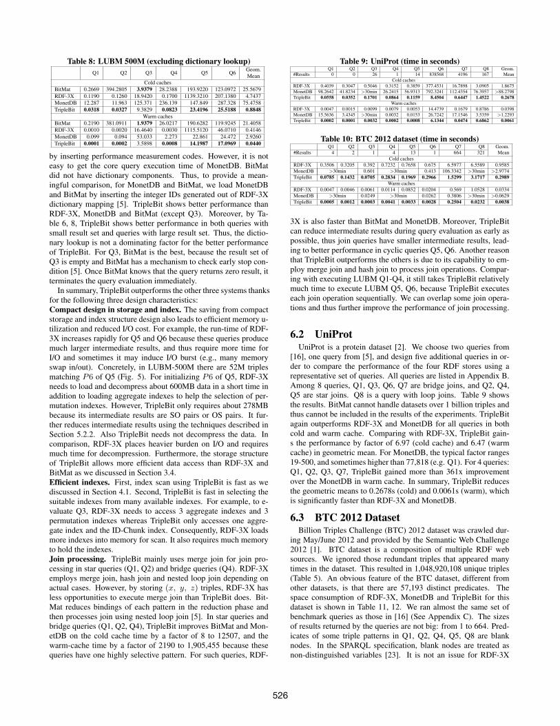
Table 8: LUBM 500M (excluding dictionary lookup)Q1 Q2 Q3 Q4 Q5 Q6 Geom.

MeanCold caches

BitMat 0.2669 394.2805 3.9379 28.2388 193.9220 123.0972 25.5679RDF-3X 0.1190 0.1260 18.9420 0.1700 1139.3210 207.1380 4.7437MonetDB 12.287 11.963 125.371 236.139 147.849 287.328 75.4758TripleBit 0.0318 0.0327 9.3829 0.0823 23.4196 25.5188 0.8848

Warm cachesBitMat 0.2190 381.0911 1.9379 26.0217 190.6282 119.9245 21.4058RDF-3X 0.0010 0.0020 16.4640 0.0030 1115.5120 46.0710 0.4146MonetDB 0.099 0.094 53.033 2.273 22.861 24.472 2.9260TripleBit 0.0001 0.0002 3.5898 0.0008 14.1987 17.0969 0.0440

by inserting performance measurement codes. However, it is noteasy to get the core query execution time of MonetDB. BitMatdid not have dictionary components. Thus, to provide a mean-ingful comparison, for MonetDB and BitMat, we load MonetDBand BitMat by inserting the integer IDs generated out of RDF-3Xdictionary mapping [5]. TripleBit shows better performance thanRDF-3X, MonetDB and BitMat (except Q3). Moreover, by Ta-ble 6, 8, TripleBit shows better performance in both queries withsmall result set and queries with large result set. Thus, the dictio-nary lookup is not a dominating factor for the better performanceof TripleBit. For Q3, BitMat is the best, because the result set ofQ3 is empty and BitMat has a mechanism to check early stop con-dition [5]. Once BitMat knows that the query returns zero result, itterminates the query evaluation immediately.

In summary, TripleBit outperforms the other three systems thanksfor the following three design characteristics:Compact design in storage and index. The saving from compactstorage and index structure design also leads to efficient memory u-tilization and reduced I/O cost. For example, the run-time of RDF-3X increases rapidly for Q5 and Q6 because these queries producemuch larger intermediate results, and thus require more time forI/O and sometimes it may induce I/O burst (e.g., many memoryswap in/out). Concretely, in LUBM-500M there are 52M triplesmatching P6 of Q5 (Fig. 5). For initializing P6 of Q5, RDF-3Xneeds to load and decompress about 600MB data in a short time inaddition to loading aggregate indexes to help the selection of per-mutation indexes. However, TripleBit only requires about 278MBbecause its intermediate results are SO pairs or OS pairs. It fur-ther reduces intermediate results using the techniques described inSection 5.2.2. Also TripleBit needs not decompress the data. Incomparison, RDF-3X places heavier burden on I/O and requiresmuch time for decompression. Furthermore, the storage structureof TripleBit allows more efficient data access than RDF-3X andBitMat as we discussed in Section 3.4.Efficient indexes. First, index scan using TripleBit is fast as wediscussed in Section 4.1. Second, TripleBit is fast in selecting thesuitable indexes from many available indexes. For example, to e-valuate Q3, RDF-3X needs to access 3 aggregate indexes and 3permutation indexes whereas TripleBit only accesses one aggre-gate index and the ID-Chunk index. Consequently, RDF-3X loadsmore indexes into memory for scan. It also requires much memoryto hold the indexes.Join processing. TripleBit mainly uses merge join for join pro-cessing in star queries (Q1, Q2) and bridge queries (Q4). RDF-3Xemploys merge join, hash join and nested loop join depending onactual cases. However, by storing (x, y, z) triples, RDF-3X hasless opportunities to execute merge join than TripleBit does. Bit-Mat reduces bindings of each pattern in the reduction phase andthen processes join using nested loop join [5]. In star queries andbridge queries (Q1, Q2, Q4), TripleBit improves BitMat and Mon-etDB on the cold cache time by a factor of 8 to 12507, and thewarm-cache time by a factor of 2190 to 1,905,455 because thesequeries have one highly selective pattern. For such queries, RDF-

Table 9: UniProt (time in seconds)Q1 Q2 Q3 Q4 Q5 Q6 Q7 Q8 Geom.

#Results 0 0 26 1 14 838568 4196 167 MeanCold caches

RDF-3X 0.4039 0.3047 0.5046 0.3152 0.3859 377.4531 16.7898 3.0905 1.8675MonetDB 98.2642 41.8234 >30min 26.2415 56.9313 792.3241 112.4354 76.3957 >88.2798TripleBit 0.0558 0.0352 0.1701 0.0864 0.1159 8.4504 0.6447 1.4522 0.2678

Warm cachesRDF-3X 0.0047 0.0015 0.0099 0.0079 0.0053 14.4739 0.1679 0.8786 0.0398MonetDB 15.5636 3.4345 >30min 0.0032 0.0153 26.7242 17.1546 3.5359 >1.2293TripleBit 0.0002 0.0001 0.0032 0.0002 0.0008 6.1344 0.0474 0.6862 0.0061

Table 10: BTC 2012 dataset (time in seconds)Q1 Q2 Q3 Q4 Q5 Q6 Q7 Q8 Geom.

#Results 4 2 1 4 13 1 664 321 MeanCold caches

RDF-3X 0.3506 0.3205 0.392 0.7232 0.7658 0.675 6.5977 6.5589 0.9585MonetDB >30min 0.601 >30min 0.413 106.3342 >30min >2.9774TripleBit 0.0785 0.1432 0.0705 0.2834 0.1969 0.2966 1.5299 3.1717 0.2989

Warm cachesRDF-3X 0.0047 0.0046 0.0061 0.0114 0.0852 0.0204 0.569 1.0528 0.0334MonetDB >30min 0.0249 >30min 0.0262 0.3806 >30min >0.0629TripleBit 0.0005 0.0012 0.0003 0.0041 0.0033 0.0028 0.2504 0.0232 0.0038

3X is also faster than BitMat and MonetDB. Moreover, TripleBitcan reduce intermediate results during query evaluation as early aspossible, thus join queries have smaller intermediate results, lead-ing to better performance in cyclic queries Q5, Q6. Another reasonthat TripleBit outperforms the others is due to its capability to em-ploy merge join and hash join to process join operations. Compar-ing with executing LUBM Q1-Q4, it still takes TripleBit relativelymuch time to execute LUBM Q5, Q6, because TripleBit executeseach join operation sequentially. We can overlap some join opera-tions and thus further improve the performance of join processing.

6.2 UniProtUniProt is a protein dataset [2]. We choose two queries from

[16], one query from [5], and design five additional queries in or-der to compare the performance of the four RDF stores using arepresentative set of queries. All queries are listed in Appendix B.Among 8 queries, Q1, Q3, Q6, Q7 are bridge joins, and Q2, Q4,Q5 are star joins. Q8 is a query with loop joins. Table 9 showsthe results. BitMat cannot handle datasets over 1 billion triples andthus cannot be included in the results of the experiments. TripleBitagain outperforms RDF-3X and MonetDB for all queries in bothcold and warm cache. Comparing with RDF-3X, TripleBit gain-s the performance by factor of 6.97 (cold cache) and 6.47 (warmcache) in geometric mean. For MonetDB, the typical factor ranges19-500, and sometimes higher than 77,818 (e.g. Q1). For 4 queries:Q1, Q2, Q3, Q7, TripleBit gained more than 361x improvementover the MonetDB in warm cache. In summary, TripleBit reducesthe geometric means to 0.2678s (cold) and 0.0061s (warm), whichis significantly faster than RDF-3X and MonetDB.

6.3 BTC 2012 DatasetBillion Triples Challenge (BTC) 2012 dataset was crawled dur-

ing May/June 2012 and provided by the Semantic Web Challenge2012 [1]. BTC dataset is a composition of multiple RDF websources. We ignored those redundant triples that appeared manytimes in the dataset. This resulted in 1,048,920,108 unique triples(Table 5). An obvious feature of the BTC dataset, different fromother datasets, is that there are 57,193 distinct predicates. Thespace consumption of RDF-3X, MonetDB and TripleBit for thisdataset is shown in Table 11, 12. We ran almost the same set ofbenchmark queries as those in [16] (See Appendix C). The sizesof results returned by the queries are not big: from 1 to 664. Pred-icates of some triple patterns in Q1, Q2, Q4, Q5, Q8 are blanknodes. In the SPARQL specification, blank nodes are treated asnon-distinguished variables [23]. It is not an issue for RDF-3X

526

Table 11: Storage space in GBLUBM

10MLUBM50M

LUBM100M

LUBM500M

LUBM1B UniProt BTC 2012

RDF-3X 0.67 3.35 6.83 34.84 69.89 145.74 81.32MonetDB 0.35 1.7 3.5 22.8 45.6 78.34 46.98TripleBit 0.42 2.39 4.88 22.01 44.5 63.81 53.08

Table 12: Storage space (Excluding dictionary) in GBLUBM

10MLUBM50M

LUBM100M

LUBM500M

LUBM1B UniProt BTC 2012

RDF-3X 0.40 2.00 4.12 21.16 42.49 98.17 43.65MonetDB 0.14 0.67 1.6 5.9 12 22.04 8.33BitMat 0.69 3.5 6.9 34.1 abort abort abortTripleBit 0.17 1.24 2.58 11.12 22.68 28.37 23.51

and TripleBit to process queries containing non-fixed predicates,but MonetDB with the vertical partitioning approach handles thispoorly [16]. The query run-times are shown in Table 10. TripleBitperforms consistently the best for all queries.

6.4 Storage spaceWe compare the required disk space of TripleBit with RDF-3X

and MonetDB in Table 11. BitMat is excluded because BitMatdoes not have the dictionary facility in its public released package.TripleBit outperforms RDF-3X for all datasets in storage space.The reason is that RDF-3X maintains all six permutations of S, Pand O in separate indexes, plus 9 aggregate indexes [17]. The s-torage of TripleBit is larger than MonetDB when loading smallerdatasets, such as LUBM-50M, LUBM-100M datasets. The rea-son is that MonetDB only stores SO pairs of RDF data. However,MonetDB requires more storage space than TripleBit when load-ing LUBM-500M, LUBM-1B and UniProt. For UniProt, TripleBitonly needs 63.81GB storage, more compact than MonetDB andsignificantly more efficient than RDF-3X since TripleBit only con-sumes 43.8% of storage required by RDF-3X. Although BTC 2012contains fewer triples than LUBM-1B, TripleBit consumes morestorage space when loading BTC 2012 than LUBM-1B for tworeasons: (i) More predicates leads to larger storage for aggregateindexes and ID-Predicate index; and (ii) strings of BTC 2012 donot share as many common prefixes as other two datasets.

Since the dictionary is usually large, Table 12 shows a compari-son of the core storage (not including storage for dictionary) among4 systems. TripleBit remains to be more compact than RDF-3Xand BitMat. BitMat has the largest storage among the four systems(BitMat experiments on LUBM-1B, UniProt and BTC 2012 abort-ed). According to Table 11, 12, the dictionary sizes of TripleBit inall data sets are smaller than the dictionary sizes of RDF-3X.

During query processing, the memory is allocated for holdingintermediate results and data structures for join processing. Forexample, RDF-3X will construct several hash tables for hash join-s. Larger intermediate results lead to larger hash tables. Thus, thesize of memory allocated for data structures used in processing joinis also highly relevant with the size of intermediate results. Wenote that intermediate results are not only the triples matching pat-terns, but also the intermediate data, such as indexes loaded intomemory during query evaluation. Table 13 shows a comparison ofTripleBit with RDF-3X and MonetDB on the peak memory usageduring the execution of LUBM Q6. LUBM Q6 is chosen becauseof its large intermediate results. Both the peak virtual and physicalmemory usage of MonetDB are the largest compared to TripleBitand RDF-3X. The query time in MonetDB also grew quickly. Tosome extent, this showed that the MonetDB process spent muchmore time in the kernel waiting for the memory pages to be al-located. Table 13 also showed that the memory consumption ofRDF and TripleBit is in proportion to the result sizes. For exam-

Table 13: Peak memory usage in GBLUBM 10M LUBM 50M LUBM 100M LUBM 500M LUBM 1B

#Results 4,462 22,001 44,190 219,772 439,997virtual phy. virtual phy. virtual phy. virtual phy. virtual phy.

RDF-3X 0.793 0.145 4.058 0.816 8.249 1.6 42.1 9.6 84.1 18MonetDB 1.577 0.851 5.104 4 10.5 8.1 44.8 40 89.3 61TripleBit 0.713 0.331 2.818 1.8 5.545 3.7 23.7 16 47.8 33

ple, the virtual memory consumption of RDF-3X in LUBM-1B isabout 2 times of its virtual memory consumption in LUBM-500M.We can find the similar phenomenon in other data sets. It is alsotrue for TripleBit. However, comparing with RDF-3X and Mon-etDB, TripleBit requires the smallest virtual memory, and the sizeof virtual memory for TripleBit grows slower than RDF-3X andMonetDB. In LUBM-1B, TripleBit’s virtual memory size is about40% of those of RDF-3X and MonetDB. These experimental re-sults show that comparing with RDF-3X and MonetDB, TripleBitcan significantly reduce the intermediate result size.

7. CONCLUSION AND FUTURE WORKWe have presented TripleBit, a fast and compact system for large

scale RDF data. TripleBit is both space efficient and query efficientwith three salient features. First, the design of a triple matrix stor-age structure allows us to utilize the variable-size integer encodingof IDs and the column-level compression scheme for storing hugeRDF graphs more efficiently. Second, the design of the two auxil-iary indexing structures, ID-Chunk bit matrix and ID-Predicate bitmatrix, allow us to reduce both the size and the number of indexesto the minimum while providing orders of magnitude speedup forscan and merge-join performance. In addition, the query process-ing framework of TripleBit best utilizes its compact storage and in-dex structures. Our experimental comparison shows that TripleBitconsistently outperforms RDF-3X, MonetDB, BitMat and deliversup to 2-4 orders of magnitude better performance for complex joinqueries over large scale RDF data.

Our work on TripleBit development continues along two dimen-sions. First, we are working on extending TripleBit for scaling bigRDF data using distributed computing architecture. Second, weare interested in exploring the potential of using TripleBit as a corecomponent of RDF reasoners [15] to speedup the reasoning usingconjunctive rules.

8. ACKNOWLEDGMENTSWe would like to thank all reviewers for their valuable sugges-

tions. The research is supported by National Science Foundationof China (61073096) and 863 Program (No.2012AA011003). LingLiu is partially supported by grants from NSF NetSE program,SaTC program and Intel ISTC on Cloud Computing.

9. REFERENCES[1] Semantic web challenge 2012.

http://challenge.semanticweb.org/2012/.[2] UniProt RDF. http://dev.isb-sib.ch/projects/uniprot-rdf/.[3] D. J. Abadi, A. Marcus, S. R. Madden, and K. Hollenbach.

Scalable semantic web data management using verticalpartitioning. In Proc. of VLDB 2007, pages 411–422. ACM,2007.

[4] S. Alvarez Garcıa, N. R. Brisaboa, J. D. Fernandez, andM. A. Martınez-Prieto. Compressed k2-triples forfull-in-memory RDF engines. In Proc. of AMCIS 2011.

[5] M. Atre, V. Chaoji, M. J. Zaki, and J. A. Hendler. Matrix bitloaded: A scalable lightweight join query processor for RDFdata. In Proc. of WWW 2010, pages 41–50. ACM, 2010.

527

[6] P. A. Bernstein and D.-M. W. Chiu. Using semi-joins tosolve relational queries. Journal of the Associanon forComputing Machinery, 28(1):25–40, 1981.

[7] V. Bonstrom, A. Hinze, and H. Schweppe. Storing RDF as agraph. In Proc. of LA-WEB 2003, pages 27–36.

[8] J. Broekstra, A. Kampman, and F. van Harmelen. Sesame: Ageneric architecture for storing and querying RDF and RDFschema. In Proc. of ISWC 2002, pages 54–68.

[9] A. Harth, J. Umbrich, A. Hogan, and S. Decker. YARS2: Afederated repository for querying graph structured data fromthe web. In Proc. of ISWC/ASWC2007, pages 211–224.

[10] O. Hartig and R. Heese. The SPARQL query graph model forquery optimization. In Proc. of ESWC 2007, pages 564–578.

[11] J. Huang, D. J. Abadi, and K. Ren. Scalable SPARQLquerying of large RDF graphs. PVLDB, 4(11):1123–1134.

[12] M. Janik and K. Kochut. BRAHMS: A workbench RDFstore and high performance memory system for semanticassociation discovery. In Proc. of ISWC 2005, pages431–445. Springer, Berlin, 2005.

[13] LUBM. http://swat.cse.lehigh.edu/projects/lubm/.[14] A. Matono, T. Amagasa, M. Yoshikawa, and S. Uemura. A

path-based relational RDF database. In Proc. of 16th ADC.[15] B. Motik, I. Horrocks, and S. M. Kim. Delta-reasoner: a

semantic web reasoner for an intelligent mobile platform. InProc. of WWW 2012. ACM, 2012.

[16] T. Neumann and G. Weikum. Scalable join processing onvery large RDF graphs. In Proc. of SIGMOD 2009, pages627–639. ACM, 2009.

[17] T. Neumann and G. Weikum. The RDF-3X engine forscalable management of RDF data. The VLDB Journal,19(1):91–113, 2010.

[18] T. Neumann and G. Weikum. x-RDF-3X: Fast querying, highupdate rates, and consistency for RDF databases. PVLDB,3(1-2):256–263, 2010.

[19] L. Sidirourgos, R. Goncalves, M. Kersten, N. Nes, andS. Manegold. Column-store support for RDF datamanagement: Not all swans are white. PVLDB,1(2):1553–1563, 2008.

[20] K. Stocker, D. Kossmann, R. Braumandl, and A. KemperK.Integrating semi-join-reducers into state of the art queryprocessors. In Proc. of ICDE 2001, pages 575–584, 2001.

[21] M. Stocker, A. Seaborne, A. Bernstein, C. Kiefer, andD. Reynolds. SPARQL basic graph pattern optimizationusing selectivity estimation. In Proc. of WWW 2008, pages595–604. ACM, 2008.

[22] SWEO Community Project. Linking open data on thesemantic web. http://www.w3.org/wiki/SweoIG/TaskForces/CommunityProjects/LinkingOpenData.

[23] W3C. SPARQL query language for RDF.http://www.w3.org/TR/rdf-sparql-query/, 2008.

[24] C. Weiss, P. Karras, and A. Bernstein. Hexastore: Sextupleindexing for semantic web data management. PVLDB,1(1):1008–1019, 2008.

[25] K. Wilkinson. Jena property table implementation. In Proc.of SSWS 2006, pages 35–46, 2006.

[26] K. Wu, E. J. Otoo, and A. Shoshani. Optimizing bitmapindices with efficient compression. ACM Transactions onDatabase Systems, 31(1):1–38, March 2006.

[27] Y. Yan, C. Wang, A. Zhou, W. Qian, L. Ma, and Y. Pan.Efficiently querying RDF data in triple stores. In Proc. ofWWW 2008, pages 1053–1054. ACM, 2008.

[28] L. Zou, J. Mo, L. Chen, M. T. Ozsu, and D. Zhao. gStore:Answering SPARQL queries via subgraph matching.PVLDB, (8):482–493, 2011.

APPENDIXA. LUBM QUERIESPREFIX r: <http://www.w3.org/1999/02/22-rdf-syntax-ns#>PREFIX ub: <http://www.lehigh.edu/∼zhp2/2004/0401/univbench.owl#>Q1-Q3: Same as Q5, Q4, Q3 respectively in [5].Q4: SELECT ?x WHERE {?x ub:worksFor <http://www.Department0.-

University0.edu>. ?x r:type ub:FullProfessor . ?x ub:name ?y1 . ?xub:emailAddress ?y2 . ?x ub:telephone ?y3 .}

Q5-Q6: Same as Q1 and Q7 respectively in [5].

B. UNIPROT QUERIESPREFIX r: <http://www.w3.org/1999/02/22-rdf-syntax-ns#>PREFIX rs: <http://www.w3.org/2000/01/rdf-schema#>PREFIX u: <http://purl.uniprot.org/core/>Q1: Same as Q6 in [5].Q2-Q3: Same as Q1, Q3 respectively in [16].Q4: SELECT ?a ?vo WHERE { ?a u:encodedBy ?vo. ?a s:seeAlso <http://-

purl.uni-prot.org/refseq/NP 346136.1>. ?a s:seeAlso <http://purl.uni-prot.org/tigr/SP 1698>. ?a s:seeAlso <http://purl.uniprot.org/pfam/-PF00842>. ?a s:seeAlso <http://purl.uniprot.org/prints/PR00992>.}

Q5: SELECT ?a ?vo WHERE { ?a u:annotation ?vo. ?a s:seeAlso <http://-purl.uniprot.org/interpro/IPR000842>. ?a s:seeAlso <http://purl.uni-prot.org/geneid/-945772>. ?a u:citation <http://purl.uniprot.org/cita-tions/9298646>. }

Q6: SELECT ?p ?a WHERE { ?p u:annotation ?a . ?p r:type uni:Protein .?a r:type <http://purl.uniprot.org/core/Transmembrane Annotation>. ?a u:range ?range . }

Q7: SELECT ?p ?a WHERE { ?p u:annotation ?a . ?p r:type uni:Protein .?p u:organism taxon:9606 . ?a r:type <http://purl.uniprot.org/core/Di-sease Annotation> . ?a rs:comment ?text . }

Q8: SELECT ?a ?b ?ab WHERE { ?b u:modified ”2008-07-22” . ?b r:typeuni:Protein . ?a u:replaces ?ab . ?ab u:replacedBy ?b . }

C. BTC 2012 QUERIESPREFIX geo: <http://www.geonames.org/>PREFIX pos: <http://www.w3.org/2003/01/geo/wgs84 pos#>PREFIX dbpedia: <http://dbpedia.org/property/>PREFIX dbpediares: <http://dbpedia.org/resource/>PREFIX owl: <http://www.w3.org/2002/07/owl#>PREFIX rdf: <http://www.w3.org/1999/02/22-rdf-syntax-ns#>Q1: SELECT ?lat ?long where { ?a [] ”Bro-C’hall” . ?a geo:ontology#in-

Country geo:/countries/#FR . ?a pos:lat ?lat . ?a pos:long ?long . }Q2: Same as Q2 in [16],Q3: SELECT ?t ?lat ?long WHERE { ?a dbpedia:region dbpediares:List of -

World Heritage Sites in Europe . ?a dbpedia:title ?t . ?a pos:lat ?lat .?a pos:long ?long . ?a dbpedia:link <http://whc.unesco.org/en/list/728>. }

Q4-Q5: Same as Q4, Q5 in [16],Q6: SELECT DISTINCT ?d WHERE { ?a dbpedia:senators ?c . ?a db-

pedia:name ?d . ?c dbpedia:profession dbpediares:Politician . ?aowl:sameAs ?b . ?b geo:ontology#inCountry geo:countries/#US . }

Q7: SELECT DISTINCT ?a ?b ?lat ?long WHERE { ?a dbpedia:spouse?b . ?a rdf:type <http://dbpedia.org/ontology/Person> . ?b rdf:type<http://dbpedia.org/-ontology/Person> . ?a dbpedia:placeOfBirth ?c. ?b dbpedia:placeOfBirth ?c . ?c owl:sameAs ?c2 . ?c2 pos:lat ?lat .?c2 pos:long ?long . }

Q8: SELECT DISTINCT ?a ?y WHERE { ?a a <http://dbpedia.org/class/-yago/Politician110451263> . ?a dbpedia:years ?y. ?a <http://xmlns.-com/foaf/0.1/name> ?n. ?b [] ?n. ?b rdf:type <http://dbpedia.org/onto-logy/OfficeHolder> . }

528