Notes on Triple Deck.

P.-Y. LagreeCNRS & UPMC Univ Paris 06, UMR 7190,

Institut Jean Le Rond ∂’Alembert, Boıte 162, F-75005 Paris, Francepyl@ccr.jussieu.fr ; www.lmm.jussieu.fr/∼lagree

October 14, 2013

Abstract

We present here briefly the famous ”triple deck theory”. In thisframework, boundary layer separation is possible without singularity.Some numerical experiments describing the flow over bumps or wedgeswithout or with flow reversal in various asymptotic regimes are pre-sented.

1 Introduction.

Let us present a summing up of the preceding chapters. We presented whathappens in a wall layer when a shear flow is disturbed, we next saw theperturbation of a Poiseuille flow. We observed in that case that pertur-bations can exist in the core flow (the Main Deck), the perturbations areexpressed as a perturbation of the stream lines trough a function −A. Wethen presented the Blasius boundary layer, we emphasized the influence ofthe displacement thickness and the retroaction with the ideal fluid in theframework of Interacting Boundary Layer Theory.

2 Triple Deck

2.1 Overview

In the fifty’s Lighthill [4] and Landau among a lot of others began to un-derstand that boundary layer separation will be explained by new scalesand a strong displacement of the boundary layer. This occurring at a smalllongitudinal scale, but larger than the boundary layer itself.

Then, simultaneously Neiland [6], Messiter [5] and Stewartson [13] in 69proposed a new asymptotic structure in three decks (figure 1).

First, there is the basic boundary layer, which is now the ”Main Deck”.this layer is disturbed near the wall where the velocity is the smaller, the

1

Triple Deck

length of this layer is small. Perturbations in this lower layer called ”LowerDeck” are transmitted through the ”Main Deck”. In this layer the pertur-bation acts as a displacement of the stream lines (with a function called−A(x)). This deflexion of the stream lines is transmitted to the ideal fluidlayer : the ”Upper Deck”. This deflexion creates a disturbance of pressure,and this disturbance of pressure will be transmitted back in the lower deckpromoting the velocity disturbances. So that we will deal with a coupledsystem of equation: a disturbance of pressure creates a disturbance of streamlines which in turn creates a disturbance of pressure.

(STEWARTSON K. & WILLIAMS P.G.1969 "Self induced separation", Proc Roy. Soc A

312, 181- 206.)

R-3/8

-5/8

-4/8

R-3/8

R

R

!3

!!

1

!"

"

!3

La synthèse se fait en partant de la solution de Blasius et en la perturbant à l'échelle !3

dégagée. Comme on est à une échelle plus courte que celle du développement de la couche

limite, le profil de Blasius (noté U0) ne varie pas en x à l'échelle considérée.

On a pour le frottement pariétal (en y=0):

dU0/dy=# !-4. et #=.3321

on écrit le développement suivant:

u=U0+!u1+...; v=!2v1+... p = !2p1

En substituant dans les ENS: on en déduit que la solution est une perturbation non visqueuse

des équations, et qu'il n'y a pas de variation transverse de pression:

u1= A(x)U0', et v1= -

d$

dx U0 et

%

%yp1=0

-dA/dx (x en !3.....) Retenons que la solution dans le "pont principal" ("Main Deck") est une

perturbation non visqueuse de la solution de Blasius.

1.2.2. pont inférieur

Près de la paroi on constate que la développement de la solution de pont principale donne:

u=#y + ! A(x)#

12 novembre 2004 "3DEATC" 3

Figure 1: Left, the triple deck scales. Right, ”triple decker ship of the line” from

HMS victory brochure Porthmouth (”vaisseau de ligne a trois ponts”). In german

”Dreierdeck-Theorie”, a french translation of Triple Deck Theory may be ”Triple

Pont” instead of ”Triple Couche”.

2.2 Scales

2.2.1 Main Deck

The classical way to look at Triple Deck is to consider perturbations of theBoundary Layer. The first idea to introduce is the existence of a perturba-tion of small length compared to the boundary layer development itself.

We have the basic non dimensional Blasius profile UB(y) in the boundarylayer, where y is the transverse variable scaled by L/

√Re. Now suppose that

at longitudinal scale say x3 there is a perturbation of this basic profile. Wewill call ”Main Deck” the region considered which is of relative scale x3 butwhich is of boundary layer scale in the transverse direction. As this scaleis small, the boundary layer as not evolved, and at first order VB = 0. So,suppose that at longitudinal scale say x3 there is a perturbation of this basicprofile of magnitude ε, then:

u = UB(y) + εu1

- IV . 2-

Triple Deck

In order to retain all the terms in the incompressibility and in the totalderivative equation,

u = UB(y) + εu1, v =ε

x3√Re

v1

longitudinal equation of momentum (UB∂u1∂x + v1U

′B), is of order ε/x3. The

previous analysis show that the relevant pressure term is in ε2/x3 which isnegligible as are the viscous terms. This small value of pressure may beconsidered here as a first hypothesis that we will verify after. The systemto solve is then

∂u1∂x

+∂v1∂y

= 0, (UB∂u1∂x

+ v1U′B) = 0,

∂p1∂y

= 0.

By elimination we find: U2B∂∂y ( v1UB

) = 0, the classical notation is then tointroduce a function of x say A(x) introduced as a constant of integration,such as

u1 = A(x)U ′B(y) and then v1 = −A′(x)UB(y)

is solution of the system.With this description, the velocity is not zero but εA(x)U ′B(0) on the

wall, so we have to introduce a new layer to full fit the no slip condition.

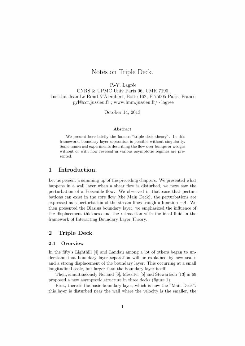
2.2.2 Lower DeckL'équilibre diffusif/ convectif doit être respecté pour assurer l'adhérence à la paroi:

u!u

!x ~ R-1

!2

!y2 u.

près de la paroi: "u ~ u ~ #3/#.

Ce qui s'écrit avec les ordres de grandeur précédents et compte tenu du fait que l'accident se

produit sur une échelle rapide x3,

"u"u/x3~"u/(#3/#)2.

Cette expression fournit l'ordre de grandeur de l'échelle rapide en fonction du rapport des

couches:

x3~(#3/#)3=$3.

On constate facilement ensuite que la pression est en $2, on admet (dans cette analyse rapide

mais on peut le montrer) qu'elle ne varie pas en y et quelle est encore inchangée au travers du

"Pont Principal" Main Deck. Cette perturbation de #3 de la couche limite produit une

déflexion des lignes de courant #3=$#. L'angle de déflexion correspondant est donc:

$#/$3.

Cette perturbation est alors ressentie par le fluide parfait comme une bosse de longueur $3 et

d'épaisseur $#. Le fluide parfait linéarisé rétroagit donc avec $3 comme échelles transverses

et longitudinales ("Pont Supérieur" Upper Deck) à cette bosse d'angle $#/$3. La perturbation

de pression de fluide parfait est donc proportionnelle à l'angle de la bosse en $#/$3. Or l'ordre

de grandeur de la pression compatible dans le Pont Inférieur est $2, donc pour qu'il y ait

rétroaction, il faut que ces deux pression soient égales:

$2=$#/$3

Ce qui donne le paramètre magique:

$=#-1/4=R-1/8.

1.2. synthèse: développements asymptotiques

1.2.1. pont principal

Il s'agit de la formulation de Stewartson 1969.

17 mai 2006 "3DEATC" 2

Figure 2: Near the wall the velocity profile is linear, the order of magnitude of

the variation of velocity must be the same than the basic flow in order to obtain

separation.

The purpose of the lower deck is to introduce a layer in which this per-turbation of velocity will be annihilated. So the scale of velocity is ε, thenas the velocity of the boundary layer is linear near the wall it is natural toguess that the lower deck will by of size εL/

√Re.

The behavior of the velocity in the Main Deck is

u = UB(y) + εA(x)U ′B(y).

- IV . 3-

Triple Deck

We look at it near the wall. For y → 0 the Blasius profile is linear nearthe wall UB(y) → U ′B(0)y and then the velocity is U ′B(0)y + εA(x)U ′B(0),written in the inner variables of the lower deck this is (as y = εy)

ε(y +A(x))U ′B(0).

So we deduce that in the lower deck the velocity should match to this quan-tity:

limy→+∞

u = (y +A(x))U ′B(0)

The convective diffusive equilibrium of the Navier Stokes equations

u∂

∂x' Re−1 ∂

2

∂y2

written with the longitudinal x3 and transversal εRe−1/2 scales reads:

ε

x3∼ Re−1 1

(εRe−1/2)2

so that the longitudinal scale is :

x3 = ε3.

The pressure is of order ε2, and the transverse equations of momentumgives as in the classical boundary layer:

∂p

∂y= 0

so, the pressure does not depend on y and is constant across the lower deck.The final system is then:

∂u

∂x+∂v

∂y= 0, u

∂u

∂x+ v

∂u

∂y= −dp

dx+∂2u

∂y2.

With no slip condition at the wall (u = v = 0), the entrance velocity profileu(x→ −∞, y) = U ′B(0)y, and the matching condition with the Main Deck:u(x, y → ∞) = (y + A)U ′B(0). Note, that the system is parabolic, there isno output condition needed to solve it.

2.3 Upper Deck

The disturbed velocity in the Main Deck is :

u = UB(y) + εA(x)U ′B(y); v =1

ε2√Re

A′(x)UB(y)

- IV . 4-

Triple Deck

and for the pressure∂p

∂y= 0

Now let us see what happens at the top of the Main Deck, for y →∞:

u = 1; v =1

ε2√Re

A′(x),

there is no more longitudinal perturbation of the velocity at order ε, butthere is a transverse velocity, a kind of ”blowing velocity” at the edge of theMain Deck. Note that the pressure remains the same order ε2.

Therefore we look at a layer of longitudinal size x3 = ε3 and of samethickness in which we have a blowing velocity at the wall of order 1√

Reε2and

a pressure of order ε2. To have a consistent problem both should be equalso that we obtain the final magic parameter:

ε = Re−1/8

3 The various regimes

3.1 Upper Deck, coupling relation incompressible

The velocity at the top of the Main Deck is then the velocity at the bottomof the upper deck: −A′. Depending on the ideal fluid regime, one maycompute the pressure. For a incompressible flow on has the Hilbert relation:

p =−1

π

∫−

dAdx

x− ξdξ

One see that there in the equations one can remove U ′0 in the equations inchanging the scales, say u multiplied by U , p is multiplied by P , x by Xand y by Y , so by invariance (u∂xu versus ∂xp) P = U2, and (u∂xu versus∂2yu) gives U = X/Y 2. At infinity u ∼ U ′0y + ... so that X = U ′0Y

3. Thepressure displacement relation tells that the pressure is proportional to A′,so U2 = Y/X which is (X/Y 2)2 = Y/X or X3 = Y 5. But remember that

X = U ′0Y3, then X = U ′0

−5/4 so, finally

x3 = (U ′0)−5/4Re−3/8, δ3 = (U ′0)

−3/4Re−5/8

u3 = (U ′0)1/4Re−1/8, v3 = (U ′0)

3/4Re−1/4, π = (U ′0)1/2Re−1/4

so that the final system is independent of the base flow.

- IV . 5-

Triple Deck

3.2 Upper Deck, coupling relation supersonic

For a compressible supersonic flow, one has the Ackeret formula:

p = −γ M√M2 − 1

dA

dx

again, changing the scales, one can remove the U ′0 :

x3 = C3/8(U ′0)−5/4(M2 − 1)−3/8Re−3/8, ...

then the relation is p = −A′.

3.3 Upper Deck, coupling relation transcritical

In transcritical flows a new parameter K = (M2 − 1)(U ′0)−2/5C−1/5Re−1/5

and

p = −(3

2√γ + 1

A′)2/3

see Bodoniy, Bartels & Rothmayer, Bodonyi and Kluwick [2].

3.4 Upper Deck, coupling relation sub/supercritical

In the case of water flow, the ideal fluid response was for the pressure thedisturbance divided by F − 1. So by rescaling:x = (x∗/L−1)U ′B(0)5 |Fr − 1|3 /(Re−3/8), y = (y∗/L)U ′B(0)2 |Fr − 1|−1 /(Re−5/8),p = (p∗/(ρU2

0 ))U ′B(0)2 |Fr − 1|−2 /(Re−2/8),p = A for subcritical flows (F < 1) and p = −A for supercritical flows(F > 1).

3.5 Jet Flow

Nearly the same configuration may exist for a wall jet of thickness δ =Re−1/2 near the wall l:

1

x3ε2u

∂u

∂x∼ ε

ε2δ2Re(∂2u

∂y2)

so that x3 = ε3 and u = U0 + εA(x)U ′0 and v = − εδx3A′(x)U0

U0∂v

∂x= −∂p

∂y, so the scale is

εδ

x23(−A′′(x))U2

0 ∼ −ε2

δ

∂p1∂y

,

so that ε = Re−1/7 which gives x3 = Re−3/7 and εδ = Re−9/14

p(x, 0) = −A′′(x)

∫ ∞0

U20 (y)dy

- IV . 6-

Triple Deck

3.6 The various regimes, canonical system

The canonical system is:

∂u

∂x+∂v

∂y= 0, u

∂u

∂x+ v

∂u

∂y= −dp

dx+∂2u

∂y2.

With at the wall (u = v = 0), at the entrance u(x → −∞, y) = y, and atthe infinity u(x, y →∞) = (y +A).

• p = −1π

∫−

dAdxx−ξdξ incompressible case

• p = −A′ supersonic

• p = −A hypersonic case

• p = A fluvial.

• p = −A torrential.

• p = −A mixed convection.

• −A = 0 pipes, Couette.

• p = −A′′ pipes, wall jets.

3.7 Linearised solution: self induced solution

We can look at a linearised solution of the canonical system. The linearisedsystem is:

∂u1∂x

+∂v1∂y

= 0, y∂u1∂x

+ v1 = −dp1dx

+∂2u1∂y2

.

With at the wall (u1 = v1 = 0), at the entrance u1(x→ −∞, y) = 0, and atthe infinity u1(x, y →∞) = A1.

We test eKx solutions on the linearized system, with K > 0.

u1 = eKxφ′(y), v1 = −eKxφ(y), p1 = eKxP

with φ(0) = φ′(0) = 0 and say φ′(∞) = 1 so that A1 = eKx; as the incom-pressibility is fulfilled, the momentum is

Kyφ′(y)− φ(y) = −KP +∂2φ′(y)

∂y2, (1)

so ∂2φ′′(y)∂y2

= Kyφ′′(y), and as φ′′(0) = KP , so φ′′ is K2/3Ai(K1/3y)P/Ai′(0)

and φ′ = K1/3PAi′(0)

∫ y0 Ai(ξ)dξ so that we deduce φ′(∞) = K1/3

3Ai′(0)P

- IV . 7-

Triple Deck

• The supersonic case allows then an eigen solution

K = (−3Ai′(0))3/4

with K = 0.827This exponential is the rational explanation of the observed self inducedseparation.• The supercitical case and the hypersonic case and the mixed convectioncase allow then an eigen solution

K = (−3Ai′(0))3

with K = 0.47

• The jet case (or pipe) allows then an eigen solution

K = (−3Ai′(0))3/7

with K = 0.89

The incompressible, the fluvial and the couette or symmetrical pipe casesdo not allow this self induced solution.

3.8 The Prandtl transform

There is a trick called ”Prandtl tranform” which allows to change the bumpywall in a flat one. One writes y = y − f(x) and keeps x = x. Then, as∂x = ∂x − f ′(x)∂y and ∂y = 0 + ∂y continuity equation becomes

∂

∂xu+

∂

∂y(v − f ′u) = 0

and as the total derivative:

u∂

∂xu+ v

∂

∂yu = u

∂

∂xu+ (v − f ′u)

∂

∂yu

so the Prandtl transform is: y = y − f(x) , x = x, u = u and v = (v − f ′u)so that system is invariant:

∂u

∂x+∂v

∂y= 0,

u∂u

∂x+ v

∂u

∂y= −dp

dx+∂2u

∂y2.

(2)

u = v = 0 on y = 0, u→ y when x→ −∞, and u→ y+f(x) when y →∞.

The sole difference lies in the boundary condition at the top.

- IV . 8-

Triple Deck

3.9 Linearised solution explicit solution in Fourier space

We can look at a linearised solution of the canonical system. The linearisedsystem is in Prandtl transform:

∂u1∂x

+∂v1∂y

= 0, y∂u1∂x

+ v1 = −dp1dx

+∂2u1∂y2

.

With at the wall (u1 = v1 = 0), at the entrance u1(x→ −∞, y) = 0, and atthe infinity u1(x, y →∞) = A1 + f1.We are looking for solutions in Fourier space so we test eikx solutions on thelinearized system.

u1 = eikxφ′(y), v1 = −eikxφ(y), p1 = eikxPk f1 = fkeikx, A1 = ake

ikx

with φ(0) = φ′(0) = 0 and then φ′(∞) = ak + fk so that; as the incompress-ibility is fulfilled, the momentum is

ikyφ′(y)− φ(y) = −ikPk +∂2φ′(y)

∂y2, (3)

so ∂2φ′′(y)∂y2

= ikyφ′′(y), and as φ′′(0) = ikPk, so φ′′ is (ik)2/3Ai((ik)1/3y)Pk/Ai′(0)

and φ′ = (ik)1/3PAi′(0)

∫ y0 Ai(ξ)dξ so that we deduce φ′(∞) = ak + fk = (ik)1/3

3Ai′(0)P

The relation between the perturbation of pressure and the displacementis then in Fourier space:

β∗FT [p] = FT [(A+ f)]

where β∗ = (3Ai′(0))−1(ik)1/3.

• The supersonic case βpf = 1/(−ik)

• The subsonic case the pressure displacement relation is βpfFT [p] = FT [(A)]with βpf = 1/ |k|

• The supercitical case is such that βpf = −1

• The fluvial case is such that βpf = 1

• The no displacement case βpf = 0.

• The no displacement case βpf = 0.

To plot the figures 3.10 one uses then the following relations:

FT [p] =FT [f ]

β∗ − βpfand FT [τ ] =

(ik)2/3

Ai′(0)Ai(0)FT [p]. (4)

and the linearized perturbation of the skin friction (τ)

- IV . 9-

Triple Deck

3.10 Plots of linearised solutions

-1

-0.5

0

0.5

1

1.5

2

2.5

3

-4 -2 0 2 4

x

Hilbert

f(x)τ(x)p(x)

-1

-0.5

0

0.5

1

1.5

2

2.5

3

-4 -2 0 2 4

x

subsonic

f(x)τ(x)p(x)

-1

-0.5

0

0.5

1

1.5

2

2.5

3

-4 -2 0 2 4

x

supersonic

f(x)τ(x)p(x)

-1

-0.5

0

0.5

1

1.5

2

2.5

3

-4 -2 0 2 4

x

p=-A

f(x)τ(x)p(x)

-1

-0.5

0

0.5

1

1.5

2

2.5

3

-4 -2 0 2 4

x

A=0

f(x)τ(x)p(x)

-1

-0.5

0

0.5

1

1.5

2

2.5

3

-4 -2 0 2 4

x

p=A

f(x)τ(x)p(x)

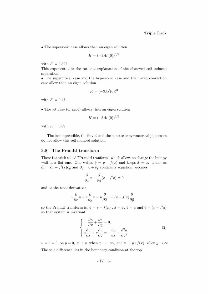
Figure 3: Friction distribution and pressure over a bump in 6 cases, linearsolution. Top left the Hilbert case, just to compare. Top right the subsonic

case p = −1π

∫−

dAdxx−ξdξ. Middle left, the supersonic p = −A′ case. Middle

right, p = −A case. Bottom left, the A = 0 case. Bottom right, the p = Acase.

- IV . 10-

Triple Deck

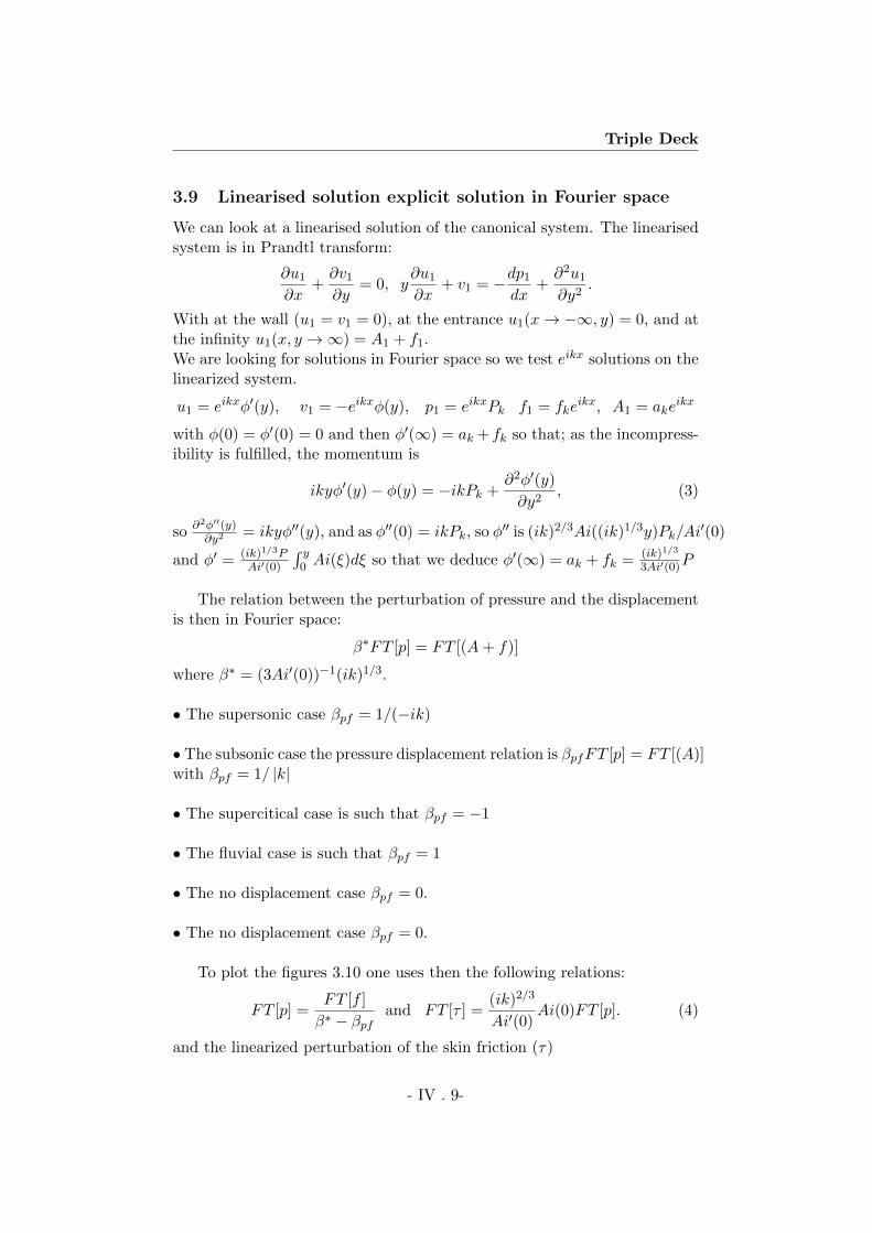
3.11 Supersonic case

Supersonic case p = −dAdx , flow over a wedge.

0

0.5

1

1.5

2

2.5

3

3.5

4

-10 -5 0 5 10

p(x)

x

α=0.5α=1.5α=2.5α=3.5

wedge

Figure 4: pressure distribution over a wedge

-0.5

0

0.5

1

1.5

-10 -5 0 5 10

τ(x)

x

α=0.5α=1.5α=2.5α=3.5

wedge

Figure 5: Friction distribution over a wedge

- IV . 11-

Triple Deck

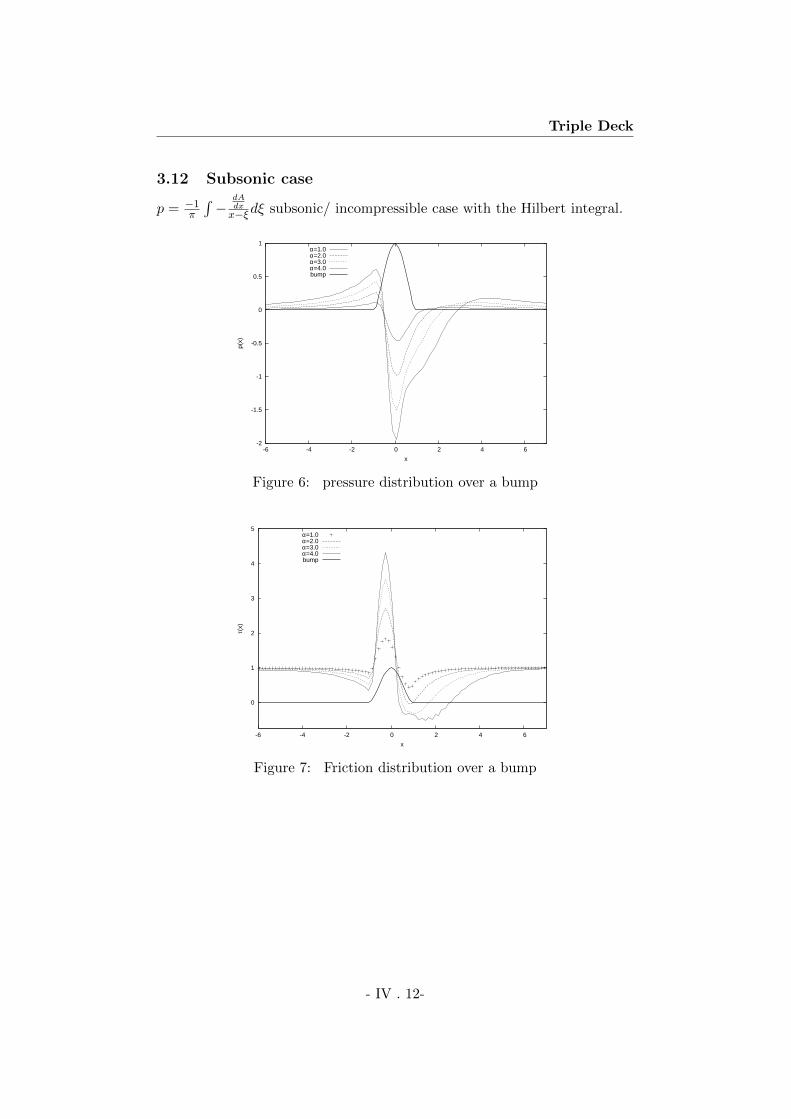
3.12 Subsonic case

p = −1π

∫−

dAdxx−ξdξ subsonic/ incompressible case with the Hilbert integral.

-2

-1.5

-1

-0.5

0

0.5

1

-6 -4 -2 0 2 4 6

p(x)

x

α=1.0α=2.0α=3.0α=4.0bump

Figure 6: pressure distribution over a bump

0

1

2

3

4

5

-6 -4 -2 0 2 4 6

τ(x)

x

α=1.0α=2.0α=3.0α=4.0bump

Figure 7: Friction distribution over a bump

- IV . 12-

Triple Deck

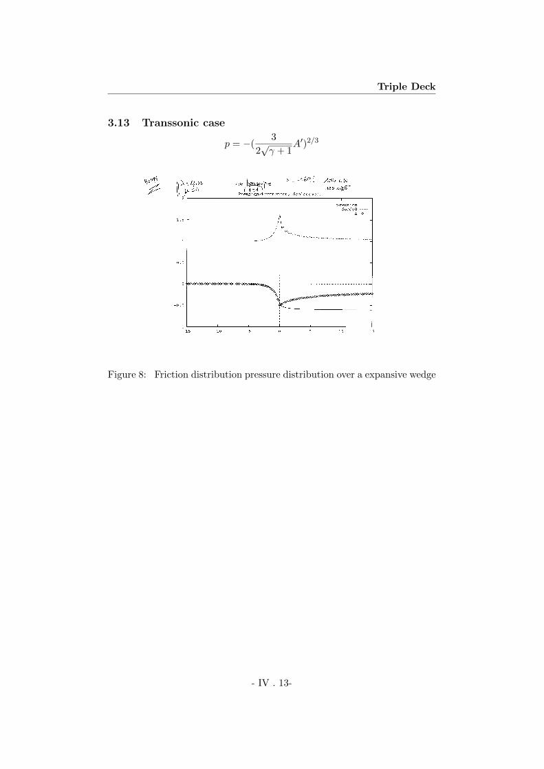
3.13 Transsonic case

p = −(3

2√γ + 1

A′)2/3

Figure 8: Friction distribution pressure distribution over a expansive wedge

- IV . 13-

Triple Deck

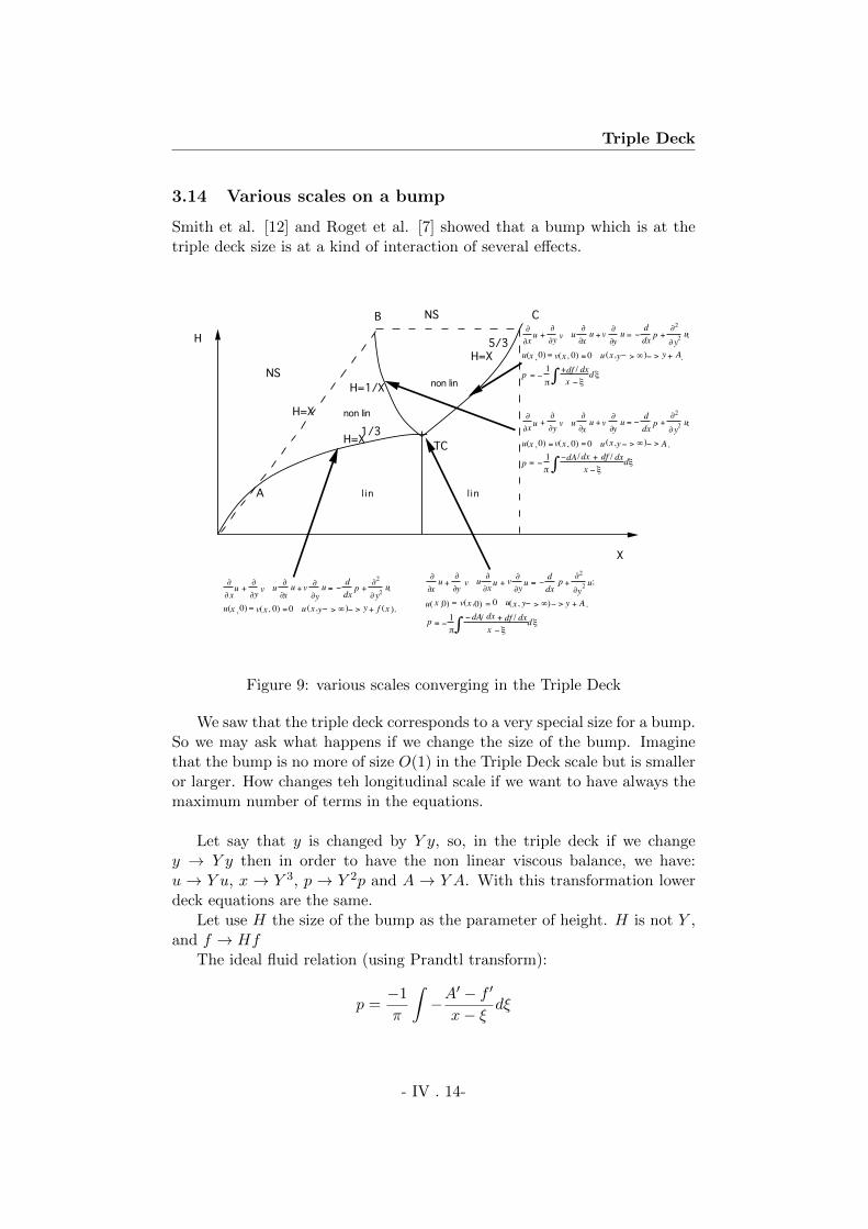
3.14 Various scales on a bump

Smith et al. [12] and Roget et al. [7] showed that a bump which is at thetriple deck size is at a kind of interaction of several effects.

TC

H

X

A

B C

!

!xu +

!

!yv u

!

!xu + v

!

!yu = "

d

dxp +

!2

!y2u;

u(x , 0) = v(x, 0) = 0 u (x,y" > #)" > y+ f (x ).

NS

!

!xu +

!

!yv u

!

!xu + v

!

!yu = "

d

dxp +

!2

!y2u;

u(x , 0) = v(x, 0) = 0 u (x,y" > #)" > y+ A.

p = "1

$

+df / dx

x "%& d%

!

!xu +

!

!yv u

!

!xu + v

!

!yu = "

d

dxp +

!2

!y2 u;

u( x ,0) = v(x,0) = 0 u(x, y" > #)" > y + A .

p = "1

$

" dA/ dx + df / dx

x "%& d%

!

!xu +

!

!yv u

!

!xu + v

!

!yu = "

d

dxp +

!2

!y2 u;

u(x , 0) = v(x, 0) = 0 u (x,y" > #)" > A .

p = "1

$

"dA /dx + df / dx

x "%& d%

NS

H=1/X

H=X

H=X

5/3

H=X1/3

l in l in

non lin

non lin

17

mai

20

06

"3

DE

AT

C"

20

Figure 9: various scales converging in the Triple Deck

We saw that the triple deck corresponds to a very special size for a bump.So we may ask what happens if we change the size of the bump. Imaginethat the bump is no more of size O(1) in the Triple Deck scale but is smalleror larger. How changes teh longitudinal scale if we want to have always themaximum number of terms in the equations.

Let say that y is changed by Y y, so, in the triple deck if we changey → Y y then in order to have the non linear viscous balance, we have:u → Y u, x → Y 3, p → Y 2p and A → Y A. With this transformation lowerdeck equations are the same.

Let use H the size of the bump as the parameter of height. H is not Y ,and f → Hf

The ideal fluid relation (using Prandtl transform):

p =−1

π

∫−A

′ − f ′

x− ξdξ

- IV . 14-

Triple Deck

has the following rescaling:

(Y 2)p = (Y −2)−1

π

∫− A′

x− ξdξ + (HY −3)

−1

π

∫− −f

′

x− ξdξ

• If now Y is large (this is a large bump X = Y 3), and if H is large,the displacement contribution decreases. for Y 2 = HY −3 i.e. H = Y 5 orH = X5/3.

The largest size of the bump is the boundary layer itself, so it gives amaximum size of Re−3/10.• If now Y is small (small bump X = Y 3), and if H is large, the displacementcontribution decreases.

(Y 4)p =−1

π

∫− A′

x− ξdξ + (HY −1)

−1

π

∫− −f

′

x− ξdξ

so H = Y and we have A′ + f ′ = 0. this is the no displacement case.

• there is a more subtle case, as the matching relation is u(x,∞) = y+A+f ,then if H is large, we may imagine that A is large (change A→ HA) and asy → Y y (with Y << H), the lower Deck is broken in two parts one where ugoes from 0 to A and another one where u = A+ f (u is of order H >> Y )so if we change A → HA, x → Xx,u → Hu and p → H2p. The ideal fluidrelation (using Prandtl transform):

p =−1

π

∫−A

′ − f ′

x− ξdξ

has the following rescaling:

(H2)p = (H/X)−1

π

∫− A′

x− ξdξ + (H/X)

−1

π

∫− −f

′

x− ξdξ

so that H = 1/X.We then have to solve:

A∂A

∂x=

1

π

∂

∂x

∫−A

′ − f ′

x− ξdξ

- IV . 15-

Triple Deck

4 Link with IBL

The IBL formulation emphasizes on the displacement thickness,

δ1 = (Re−1/2)

∫ ∞0

(1− u(x, y))dy

we have to decompose it into two parts as we cross the lower and the maindecks. Let introduce Y

δ1 = (Re−1/2)(

∫ Y

0(1− u(x, y))dy +

∫ ∞Y

(1− u(x, y))dy)

the first integral is estimated near the wall, so the Lower Deck description(y = εy) is valid there, but a good idea is to write the velocity u(x, y) =U ′B(0)(y +A) + uc where uc is a correction:

(

∫ Y

0(1− u(x, y))dy) = ε(

∫ Y /ε

0(1− ε(U ′B(0)(y +A)))dy −

∫ Y /ε

0εucdy)

the second one is in the Main Deck∫ ∞Y

(1− u(x, y))dy =

∫ ∞Y

(1− UB(y)− εA(x)U ′B(y))dy.

Re summing the two integrals and changing the order of the terms allowsthen write:

δ1 = (Re−1/2){[ε(∫ Y /ε

0(1− ε(U ′B(0)(y)))dy +

∫ ∞Y

(1− UB(y))dy]+

+[ε(

∫ Y /ε

0(−ε(U ′B(0)(A)))dy +

∫ ∞Y

(−εA(x)U ′B(y))dy]− ε2∫ Y /ε

0ucdy)}

so that we recognise :

δ1 = (Re−1/2){∫ ∞0

(1−UB(y))dy+

∫ ∞0

(−εA(x)U ′B(y))dy−ε2∫ Y /ε

0ucdy)}.

or

δ1 = (Re−1/2){∫ ∞0

(1− UB(y))dy − εA(x)−O(ε2)}.

the −εA contribution of the triple deck is the perturbation of the displace-ment thickness

∫∞0 (1 − UB(y))dy. So the IBL technique based on δ1 is

justified by the triple deck analysis.

5 ∂’Alembert Paradox and Kutta condition

At this point, it is time to introduce the famous d’Alembert Paradox. Thetriple deck structure is a possible response to solve it. The Kutta conditiondoes not exist, the flow can turn round the trailing edge, but this is at aRe−3/8 scale, it is so small when Re→∞ that this gives the Kutta condition.

- IV . 16-

Triple Deck

6 Conclusion

In this chapter we presented the Triple Deck scales and equations. Weshowed that there is an interactive problem between a thin layer near thewall and a layer of ideal fluid through the displacement of the stream lines−A. In the thin layer, Prandtl equations are valid with new scales, and adifferent matching condition involving this displacement function −A. Theupper layer Euler small disturbance theory applies, the layer in between isthe boundary layer which is passive and only transmits the perturbations of−A and pressure p. This framework allows to understand boundary layerseparation and self induced separation. The pressure deviation relation pres-sure p displacement −A allows a large variety of various coupled problems...

References

[1] Cebeci T. & Cousteix J. (1999): “Modeling and computation of bound-ary layer flows“, Springer Verlag.

[2] Bodonyi and Kluwick, (1977): ”Freely interacting transonic boundarylayers”. Phys. Fluids 20 (1977), pp. 1432–143

[3] Gajjar J. & Smith F.T. (1983): ”On hypersonic self induced separation,hydraulic jumps and boundary layer with algebraic growth”, Mathe-matika, 30, pp. 77-93.

[4] M.J. Lighthill (1953) : On boundary-layer and upstream influence : II.Supersonic flows without separation. Proc. R. Soc., Ser. A 217 :478–507

[5] A.F. Messiter (1970): Boundary–layer flow near the trailing edge of aflat plate. SIAM J. Appl. Math., 18 :241–257,

[6] Neiland V. Ya (1969): ”Propagation of perturbation upstream withinteraction between a hypersonic flow and a boundary layer”, Mekh.Zhid. Gaz., Vol. 4, pp. 53-57.

[7] C. Roget, J. Ph. Brazier , J. Cousteix and J. Mauss (1998): ”A contri-bution to the physical analysis of separated flows past three-dimensionalhumps” European Journal of Mechanics - B/Fluids Volume 17, Issue 3,May-June 1998, Pages 307-329

[8] Ruban A.I. & Timoshin S.N. (1986): “Propagation of perturbations inthe boundary layer on the walls of a flat channel“, MZG 2, pp. 74-79.

[9] Saintlos S. & Mauss J. (1996): ”asymptotic modelling for separatingboundary layers in a channel”, Int. J. Engng. Sci.,Vol 34, No 2, pp201-211.

- IV . 17-

Triple Deck

[10] Smith F. T. (1976): ”Flow through constricted or dilated pipes andchannels”, part 1 and 2, Q. J. Mech. Appl. Math. vol 29, pp 343- 364& 365- 376.

[11] Smith F. T.(1982): ”On the high Reynolds number theory of laminarflows”, IMA J. Appl. Math. 28 207-81.

[12] Smith FT, Brighton PW M., Jackson PS & Hunt JCR ”On boundarylayer flow past wo dimensional obstacles”, JFM 110, pp 1-37 (1981).

[13] Stewartson K. & Williams P.G. (1969): ”Self - induced separa-tion”,Proc. Roy. Soc. London, A 312, pp 181-206.

[14] Stewartson K. (1974): ”Multistructured boundary layer on flat platesand related bodies” Advances Appl. Mech. 14 p145-239.

[15] Sychev V. V. , Ruban A. I. , Sychev V. V. & Korolev G. L. (1998):”Asymptotic theory of separated flows”, Cambridge University Press.

[16] http://cis.jhu.edu/∼tilak/blsep.html

The web page of this text is:http://www.lmm.jussieu.fr/∼lagree/COURS/CISM/

The last version of this file is on:http://www.lmm.jussieu.fr/∼lagree/COURS/CISM/TriplePont−CISM.pdf

This file consist in notes for the CISM Course ”ASYMPTOTIC METH-ODS IN FLUID MECHANICS: SURVEY AND RECENT ADVANCES”,Advanced School coordinated by Herbert Steinruck Udine, September 21 -25, 2009.P.-Y . L agree’ s contribution is:http://www.lmm.jussieu.fr/ lagree/COURS/CISM/IVIIBL−CISM.pdf

- IV . 18-