Department of Economics Trinity College Hartford, CT 06106 USA

http://www.trincoll.edu/depts/econ/

TRINITY COLLEGE DEPARTMENT OF ECONOMICS

WORKING PAPER 10-06

Foreign Direct Investment and its Determinants in the Chilean Case: Unit Roots, Structural Breaks, and Cointegration Analysis.

Miguel D. Ramirez

Abstract

This paper examines the major economic and institutional factors underlying the surge in foreign direct investment (FDI) flows to Chile during recent decades. It presents econometric evidence for the 1960-2003 period which indicates that market-based economic reforms and major changes in the institutional-legal status of foreign capital are, in large measure, responsible for the rapid increase in FDI inflows to leading sectors of the Chilean economy. Single break unit root and cointegration analysis suggest that market size, the real exchange rate, the debt-service ratio, the secondary enrollment ratio, physical infrastructure, and institutional reforms such as the elimination of restrictions on profit and dividend remittances and the implementation of a selective debt conversion program are economically significant in explaining the variation in FDI inflows to the country. The paper also addresses the long-term negative effects which rapidly growing profit and dividend remittances may have on the financing of capital formation and the Chilean balance of payments. JEL codes: C22, O10, O40, O57. Keywords: Akaike Information Criterion (AIC); Chilean economy; cointegration analysis; error correction model; FDI flows; Granger causality test; Johansen and Juselius test; remittances of profits and dividends; Structural breaks and unit roots; Theil inequality coefficient; Zivot and Andrews one-break unit root test.

brought to you by COREView metadata, citation and similar papers at core.ac.uk

provided by Research Papers in Economics

1

I. Introduction.

During the decade of the nineties, foreign direct investment (FDI) undertaken by transnational

corporations (TNCs) became one of the leading factors in promoting the process of economic

globalization. Between 1985 and 1990 these flows averaged $142 billion on an annual basis,

while during the 1991-2004 period alone they averaged $392 billion, or more than twice as much

[see ECLAC, 2004]. The acceleration in FDI flows during the 1990s and early 2000s was also

characterized by an increasing proportion of these funds directed to the developing nations,

including the countries of Latin America and the Caribbean. From a relative standpoint, Latin

America=s share of FDI flows to developing countries rose from 29 percent in 1995 to an-all time

high of 39.5 percent in 2000, before falling to 33.3 percent in 2004, mainly confined to

Argentina, Brazil, Colombia, Chile and Mexico (UNCTAD, 2007). Part of the reason for the fall

in the share of FDI flows to the region in recent years can be explained by the economic

recession in the United States in 2001-02 and the completion of major privatizations in industry,

banking, and mining (see UNCTAD, 2007).

The increase in net FDI flows channeled to these countries, particularly Chile, has been

nothing short of spectacular when you factor in the relatively small size of Chile’s economy.

Between 1989 and 1994 Chile averaged FDI inflows of $1.2 billion, while during the 1995-2006

period it raised its average more than fourfold to $5.6 billion [ECLAC, 2008]. During the latter

period, Chile ranked only behind Brazil ($18.1 billion) Mexico ($14.2 billion) and Argentina

($6.3 billion)--much larger economies--in its ability to attract net FDI inflows [ECLAC, 2007].

The extant literature contends that, in large part, this has been due to Chile’s relatively successful

implementation of macroeconomic stabilization measures and structural reform programs. The

2

former have insured high and sustained rates of economic growth with relatively low inflation

rates since 1985, while the latter have taken the form of privatization and debt conversion

programs, the liberalization of the tradeable sector, and the removal of overly restrictive FDI

legislation concerning the repatriation of profits as well as local content and export requirements.

The adoption of these fiscally prudent and structural reform policies has reassured both foreign

and domestic investors in the country’s commitment to market-based, outward-oriented reforms

[see Edwards, 1999]. Critics, however, contend that the rapid and far-reaching liberalization of

the tradeable sector was undertaken with little or no regard to its negative impact on domestic

industry, employment, and the environment; moreover, they contend that the removal of

restrictions on the remittances of profits and dividends has generated in recent years a growing

reverse flow to parent companies which has become a significant constraint on the balance of

payments [see Ffrench-Davis, 1999; Green, 2003; and Meller, 1993]. Only time will tell if these

reforms are sustainable in the long run, particularly in the wake of recent economic and financial

crises that have buffeted the region. What is indisputable, however, is that FDI flows will not

only play a strategic role in modernizing Chile’s-- and Latin America’s-- economy, but in

providing future income and employment opportunities.

In view of the above, this paper analyzes the recent evolution, rationale, and major economic

and institutional determinants of FDI flows to Chile. Chile was one of the earliest countries in

the region to adopt and implement market-based reforms, albeit at great social and political cost.

The process of economic and financial liberalization began following the brutal military coup of

1973 and, in recent years, Chile has further liberalized its FDI regime by modifying Decree Law

600 and its debt capitalization mechanism (Chapter XIX of the Central Bank’s Compensation of

International Exchange Regulations). FDI flows in the Chilean case have, historically, been

3

channeled to traditional sectors such as mining and energy sectors. However, with the return of

democracy during the nineties, a significant proportion of these funds have been channeled to

export-oriented manufacturing operations or to non-traditional sectors using innovative

technological processes and managerial techniques. An analysis of the evolution and

determinants of FDI flows to Chile during the decade of the nineties and beyond should uncover

important trends and provide valuable policy insights to government officials seeking to attract

these flows to the country.

The layout of the paper is as follows: First, it reviews the extant literature on the major

economic and institutional determinants of FDI. Second, the paper gives an overview of FDI

flows to Chile in terms of their absolute magnitude and relative contribution to the financing of

private capital formation. Third, the paper presents unit root tests with and without structural

breaks as well as cointegration and error-correction model results that identify some of the major

economic and institutional determinants of FDI flows to Chile during the 1960-2003 period. The

concluding section summarizes the major arguments and offers some policy prescriptions for

attracting FDI into the region and enhancing its positive direct and indirect effects.

II. Conceptual Framework.

From a theoretical standpoint, John Dunning [1981; 1988] has developed one of the most

comprehensive explanations of why TNC firms undertake cross-border investments. He argues

that TNCs invest abroad when three sets of relative advantages are present. First, the

establishment of TNC subsidiaries gives the parent firms exclusive ownership rights over

patents, trademarks, commercial secrets and production processes, thereby effectively denying

access to both foreign and domestic competitors. Second, they generate for TNC affiliates

locational advantages that arise from direct access to growing markets and lower unit labor costs,

4

reduced transportation and communication costs, avoidance of tariffs and non-tariff barriers, and

last but not least, direct access to raw materials, low-cost unskilled labor, and intermediate

products that are indispensable for the production of certain goods. Michael Mortimore (2003),

building on Dunning’s work, argues that the relative importance of location specific

determinants depends on TNC motivations for investing, viz., whether FDI is motivated by

market-seeking (access to internal and export markets), natural resource-seeking (access to

natural resources and low-cost labor) or efficiency-seeking reasons (cost and quality of human

resources and physical infrastructure resources).

Third, Dunning points to the advantages TNCs derive from internalizing certain operations

because utilizing market mechanisms are relatively more burdensome and costly. For instance,

many TNCs would rather establish a subsidiary abroad and assume directly the contractual and

administrative costs associated with research, development, production, and marketing of a given

product or service, thereby avoiding the transaction costs associated with leasing licenses and

securing patents to undertake production or hiring the services of advertizing agencies to market

and distribute their products. In this connection, Markusen (1995) argues that firms choose direct

investment rather than licensing primarily because of the non-excludability property of new

knowledge capital; viz., it is too costly for TNCs to prevent licensees from “defecting” and

copying the new technology at little cost and setting up their own domestic firms in direct

competition with the TNCs (p. 182).

Host country determinants also seem to play a very important role in either attracting or

discouraging FDI flows to developing countries. For example, countries that exhibit a greater

degree of political and macroeconomic stability, the existence of well-defined and enforceable

5

property rights when it comes to the transfer of technology, liberal legislation governing the

remittance of profits and dividends, and limited or non-existent local content or export

requirements tend, on average, to attract greater flows of FDI. However, from the standpoint of

the host country the very factors which act as an incentive for FDI flows in the short run may

prove detrimental to long-term economic development if they lead to a net outflow of resources,

few backward and forward linkages, and limited transfers of technology and managerial

knowhow [see Blomstrom and Persson, 1983; Dietz and Cypher, 2003; Kolko and Zejan, 1996;

and Yeager, 1998 ].

The nature and scope of government policies are also a highly important factor in determining

whether FDI flows to developing economies such as Chile. For example, FDI is likely to be

attracted to countries where governments ensure an adequate provision of economic and social

infrastructure in the form of paved roads, ports, airfields, relatively cheap energy supplies, and a

well-educated and disciplined work force. In this connection, several investigators have found

that the availability of skilled workers and adequate physical infrastructure are important

determinants of FDI flows because it enables TNCs to strengthen both their ownership and

locational advantages, thus allowing them to expand their market not only in the host country but

the region as well [see Ramasamy and Young, 2004; and Zhao and Zhu, 2000]. In addition, FDI

flows are likely to be encouraged by government policies that lead to the establishment of a

legal-institutional framework that is conducive to business activity; viz., one that significantly

reduces the transactions costs associated with negotiating contracts, improves information about

the quality of goods and services, and make sure that the parties to a formal agreement honor

their commitments [see North, 1990; and Yeager, 1998].

6

Finally, changes in a country’s exchange rate policy play a key role in altering its relative

attractiveness to net FDI inflows. Not surprisingly, economists are not entirely of one mind when

it comes to the optimal exchange rate strategy to pursue. For example, some investigators argue

that a policy that keeps the real exchange rate undervalued relative to that of its key investment

partners is, ceteris paribus, likely to enhance FDI flows because it artificially reduces the unit

costs of the country’s factors of production and thus enables investors to make a significantly

larger investment in terms of the domestic currency. They also contend that it enhances the

profitability of the export-oriented sector which, in turn, attracts FDI flows to them. Therefore,

the amount of FDI should increase with a real devaluation of the domestic currency after a

reasonable lag [see ECLAC, 1998; De Vita and Lawler, 2004].

Other researchers contend that a policy that leads to a real appreciation of the domestic

currency is likely to encourage FDI inflows because it enhances the foreign currency (dollar)

value of the remittances of profits and dividends back to the parent company [see De Mello, Jr.,

1997; and De Vita and Lawler, 2004]. After all, it is the real rate of return on their initial (dollar)

investment that matters to the parent company. In light of the conflicting views in the literature

on the impact of the exchange rate on FDI flows, it is best, from a policy standpoint, to pursue a

credible strategy that maintains the country’s real exchange rate in line with that of its key

trading and investment partners.

III. FDI Flows to Chile.

The lost decade of the 1980s led to an absolute decrease in net FDI inflows to Latin America

and the Caribbean during the first half of the 1980s, after which they began to increase steadily

7

during the second half of the 1980s and posted a dramatic upward surge during the decade of the

1990s. FDI flows to the countries of Latin American rose from $8.4 billion in 1990 to an all-

time high of 80 billion in 1999, before retreating to $72.2 billion in 2000 and falling

precipitously to $ 38.3 billion in 2003 as a result of the U.S. recession and the completion of

major privatizaions. With the recovery of economic activity in the United States after 2003, FDI

flows to the countries of Latin American and the Caribbean began to recover as attested by the

sharp rise in net flows to $53.7 billion in 2005 and $84.7 billion in 2007 [ECLAC, 2008, Table

A-1, p. 149].

The strength of these flows is revealed by the fact that despite the serious economic downturn

in Mexico in 1995, and the associated “Tequila effect” which reduced FDI flows to Latin

America relative to 1994Band the aforementioned effects of the 2001-02 U.S. recession-- they

managed to stage a remarkable recovery during the ensuing post-crises years. In absolute terms,

the major recipients of FDI flows have been concentrated in a few major countries of the region,

in order of importance of the cumulative level of inflows during the 1990-2003 period, they are

Brazil, Mexico, Argentina, Chile and Venezuela. The major supplier of FDI flows to Latin

America during the decade of the nineties (and historically) has been the United States followed,

in order of importance, by Great Britain, Japan, Germany, and France [see ECLAC, 2005]

In relative terms, the major countries of Latin America, particularly Chile and Mexico, have

exhibited a consistently strong record of attracting FDI inflows during the decade of the 1990s,

never falling below 1.5 percent of their countries’ respective GDPs, and beginning in 1994, FDI

inflows have averaged 5.4 percent in the case of Chile [computed from ECLAC, 1995; 2005].

The importance of these inflows is more fully appreciated by focusing on their evolution relative

8

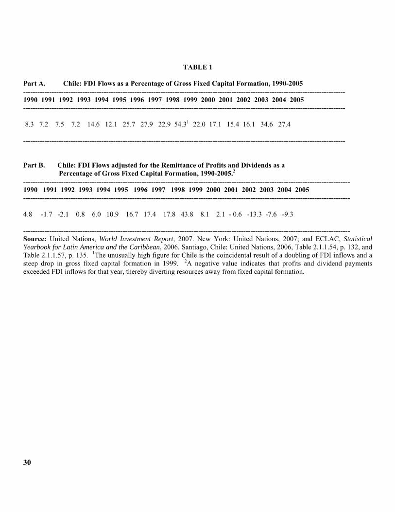
to these countries’ gross fixed capital formation. Table 1 (part A) shows that throughout the

decade of the 1990s, and particularly after 1993, FDI flows now represent more than 15 percent

of their countries’ gross fixed capital formation, and in the case of Chile during 1996, 1997,

1999, and 2005, they reached more than a quarter of gross fixed capital formation--the highest

figure among the major countries of the region, or for that matter, the developing world.i

(Table 1 about here)

Critics of FDI , however, contend that instead of increasing the investable resources of the

host nation, FDI flows divert resources away from capital formation because they generate a

substantial reverse flows in the form of remittances of profits and dividends to the parent

companies, as well as through the widespread practice of intra-firm transfer pricing [see Cypher

and Dietz, 2003; Kahai, 2004; Plasschaert, 1994; and Ram and Zhang, 2002]. In their view, in

order to assess the net contribution of FDI to the financing of private capital formation, one must

first deduct from gross FDI inflows the repatriation of profits and dividends to the parent

companies, often residing in the U.S. for many of the countries in question.

Partial support for this contention can be surmised from the following figures: profit and

dividend remittances by Latin America and the Caribbean to the developed countries more than

quadrupled between 1990 and 2005, from $7.0 billion to over $37.2 billion [see ECLAC, 2006,

Table 15, p. 143. Chile’s remittances of profits and dividends registered more than a twenty fold

increase between 1990 and 2005, from $400 million to $9.3 billion [ECLAC, 2006, p. 175]!

Relative to the inflows of FDI during the 1990-2005 period, Chile’s remittances of profits and

dividends averaged 55 percent of total FDI flows over the same period. If we subtract profits

and dividends from FDI flows and express the net figure as a proportion of fixed capital

9

formation, it is evident from Table 1 (part B) that the net contribution of FDI inflows to gross

fixed capital formation to Chile, although increasing in recent years, is far less than that

advertised for the unadjusted figures. The table shows that there was a diversion of economic

resources away from financing fixed capital formation during the 1992-93 period, and an even

more significant one during the recent 2002-05 period.

Economic theory, however, suggests that rather than focus on the flows of FDI to the

countries of Latin America, it is theoretically more appropriate to concentrate on the

accumulated stock of FDI, because increases in the latter raise the host country=s marginal

productivity of private capital (and labor), a process that eventually translates into higher levels

of output, employment creation, and potential tax revenues [see Bosworth and Collins, 1999].

The stock of FDI in Latin America (1990 dollars) rose from $175.6 billion in 1990 to $462

billion in 2003 [ECLAC, 2004, p. 760]. This represents more than a doubling in the stock of FDI

of these countries, an increase which is far greater than that of the entire “lost decade” of the

1980s. In this connection, Chile’s performance was even more impressive in view of the fact that

its stock of FDI rose from $1.7 billion in 1990 to a level of $11 billion by year-end 2003, or more

than six times [ECLAC, 1995; 2007]. From a relative standpoint, Chile’s stock of FDI as a

percentage of GDP more than doubled between 1990 and 2003, from 5 percent to 13.9 percent in

2003 [ECLAC, 1995; and 2007]. In addition to the direct effects associated with a greater stock

of FDI, several investigators contend that there are indirect positive spillover effects on overall

efficiency that arise from enhanced competition generated by foreign firms, the transfer of

needed technology and managerial knowhow to local firms, and trade-induced learning-by-doing

10

effects as local firms attempt to overcome competition in the global market [see De Mello Jr.,

1997; Huang, 2004; and Ram & Zhang, 2002].

IV. Empirical Model and Results.

From an historical standpoint, empirical work on the determinants of FDI flows to Latin

America and the Caribbean have been relatively few given the paucity and inconsistency of the

data, as well as the economic and institutional heterogeneity present in these countries. However,

in recent years, a number of studies focusing on the determinants (and impact) of FDI flows to

several countries of the region have arisen as a result of the renewed surge in net flows to these

countries beginning in the second half of the 1980s and the availability of reliable and

methodologically consistent time series data for a number of countries [see Agosin, 1995;

Bloomstrom and Wolff, 1994; DeMello, Jr., 1997; ECLAC, 2000; Figueroa, 1998; Ramasamy

and Yeung, 2004; Ramirez, 2000; Ros, 1994; and Zhang, 2001].

Model.

Following the lead of Agosin [1995], [Ramasamy and Yeung, 2004], Ros [1994] and Zhang

[2001], this study estimated a foreign direct investment (FDI) function of the following general

form:

FDI t = f(GDPt-i, REXt-i, DSt-i , SEDt-i , PAVEDt-i ; Di) + εt (1)

It includes standard arguments such as real GDP, the real exchange rate (REX), the ratio of debt

service payments to exports of goods and services (DS), the number of students enrolled in

secondary education (SED) as a proxy for human capital, the total kilometers or the percentage

of paved roads as a proxy for physical infrastructure, and dummy variables (Di) to explain the

11

variation in FDI flows to Chile during the 1960-2003 period.ii εt is a normally distributed error

term. Chile’s potential market size is proxied by the lagged value of real GDP because foreign

investors make their investment decisions based on expectations generated, in part, by what the

level of real GDP was in the preceding year. The sign associated with this variable is expected to

be positive. Market size was also proxied by the value of real exports (X) in view of the growing

importance of external markets for the Chilean economy since 1987. For example, the data

indicate that after 1987 a significant share of the country’s GDP (at least 25 percent and as high

as 35 percent in 2000-2001) has been destined for export markets in the high income OECD

(Europe, U.S. and Japan) countries and China [see Banco de Chile, pp. 368-9; OECD, 2003,

Table A.1].

The real exchange rate is included in the model because it is the most important link between

economic policy and international competitiveness and, as explained in Section II, it is expected

to have an indeterminate sign in the Chilean case.iii On the one hand, a considerable proportion

of FDI flows to Chile, in recent years, are concentrated in foreign affiliates which have a strong

export orientation, such as cellulose and paper, telecommunications, and manufacturing. A

ceteris paribus real depreciation of the domestic currency (a rise in REX) should increase the

profitability of these sectors and, ceteris paribus, induce FDI flows to them. On the other hand, a

real depreciation of the domestic currency reduces the (dollar) value of the remittances of profits

and dividends back to the parent company, thereby reducing the real rate of return on the parent

company’s initial (dollar) investment. According to this rationale, a ceteris paribus depreciation

of the domestic currency should reduce FDI flows to the country. This variable is introduced

12

with a lag because the decision to invest in new plant, machinery, and equipment in a foreign

country takes time due to recognition, implementation, and institutional-legal delays.

The debt service payments- to- exports ratio, was included to measure country risk; viz., the

higher the ratio, the greater the probability that a BOP crisis will emerge which may lead to the

imposition of restrictions on profit and dividend remittances, thereby depressing FDI flows to the

country. This variable is also designed to capture the influence of external factors on the Chilean

economy, such as the increase in the cost of credit and/or demand for the country’s exports. It is

anticipated to have a negative and statistically significant effect on inward FDI flows.

The final quantitative variables, the number of students enrolled in secondary education

(thousands) and the kilometers of paved roads (hundreds), were included, respectively, as crude

proxies for the quality of the country=s human and physical capital. Insofar as the education

variable is concerned, it would have been preferable to have used the secondary enrollment ratio,

but this variable was not available for the entire period. In the case of the physical infrastructure

variable, the percentage of paved roads was also utilized and, as reported below, the results were

not significantly different. The rationale for including these variables is relatively

straightforward. For example, it is hypothesized that, ceteris paribus, the higher the level of

education in the country, the more attractive it is to foreign investors both from a cost standpoint

(lower unit labor costs) and a demand-side perspective (greater purchasing power and more

informed consumers). In the case of physical infrastructure, it is hypothesized that the higher the

percentage of paved roads in the country, the more attractive it is to TNCs because it allows them

to move resources and distribute goods at lower cost [see Ramasamy and Yeung, 2004].

13

Turning to the qualitative variables, dummy variable D1 equals 1 for the political crises years

of 1970-1973 (administration of president Salvador Allende Gossens and 1973 military coup),

and 1988-90 (transition to democratic rule), and 0 otherwise; this variable is anticipated to have a

negative and statistically significant effect on foreign (and domestic) investment because of the

uncertainty generated for expected returns from political turmoil and depressed economic

activity. Again, these events may induce government officials to adopt a more nationalistic

stance and impose restrictions on foreign investors in terms of the sectoral destination of FDI

flows and the repatriation of profits and dividends. D2 is set equal to 1 for the 1987-97 period

(acceleration of real economic growth associated with the Chilean government’s decision to

pursue vigorously an outward-oriented strategy of economic development beginning in 1986-87.

D3 equals 1 for the debt-led growth years of 1978-81. Both D2 and D3 are expected to have

positive and statistically significant coefficients. The model was also estimated with dummy

variable D2 multiplied by real GDP. By estimating this variable interactively with real GDP one

can assess whether the consolidation of market-oriented reforms had a positive and significant

effect on the capacity of market size to affect real FDI flows.

Data

Economic data (including foreign direct investment) used in this study were obtained from

official government sources such as the Instituto Nacional de Estadisticas (various issues), the

Banco Central de Chile;s Memoria Anual (various issues) and the Banco’s comprehensive

longitudinal publication entitled, Indicadores Economicos y Sociales, 1960-2001 [August 2003

14

Excel edition]; data was also obtained from the OECD’s recent publication entitled, OECD

Economic Surveys 2003: Chile and UNCTAD, World Investment Report 2003.iv The FDI stock

variable (KDI) in millions of 1977 pesos was generated using a standard perpetual inventory

model. Initial stocks of private foreign capital were estimated by aggregating over four years of

gross investment (1957-1960), assuming an estimate of the rate of depreciation of 5 percent.v

GDP is real gross domestic product in millions 1977 pesos. REX is the real exchange rate

(1978=100), where an increase represents a real depreciation of the domestic currency. DS is the

ratio of debt-service payments- to- exports of goods and services variable; debt-service payments

include both amortization (gradual payment of principal) and interest payments on the country’s

total external public debt. SED refers to the number of students matriculated in secondary

education, and PAVED is defined as the total number of paved roads (in kilometers).

Structural Breaks and Unit Root Analysis.

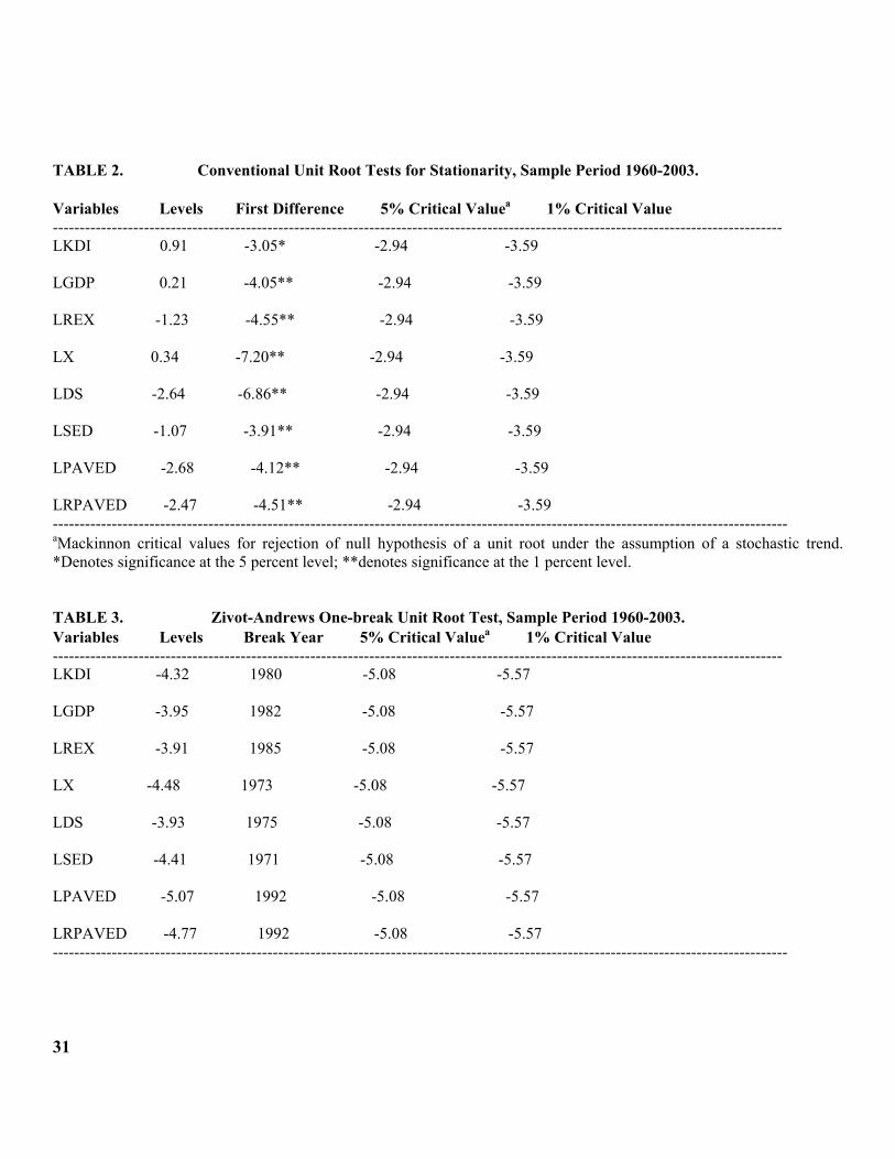
Initially, conventional unit root tests (without a structural break) were undertaken for the

variables in question given that it is well-known that macro time series data tend to exhibit a

deterministic and/or stochastic trend that renders them non-stationary; i.e., the variables have

means, variances, and covariances that are not time invariant. Engle and Granger [1987] have

shown that the direct application of OLS or GLS to non-stationary data produces regressions that

are mispecified or spurious in nature. Table 2 below presents the results of running an

Augmented Dickey-Fuller test (one lag) for the log of the variables in both level and differenced

form under the assumption of a stochastic trend.vi It can be seen that the variables in level form

are non-stationary. In the case of first differences, however, the null hypothesis of non-

stationarity (unit root) can be rejected for the relevant variables at least at the five percent level.

15

(Table 2 about here)

Although suggestive, the conventional results reported in Table 2 may be misleading because

the power of the ADF test may be significantly reduced when the stationary alternative is true

and a structural break is ignored (see Perron, 1989); that is, the investigator may erroneously

conclude that there is a unit root in the relevant series. In order to test for an unknown one-time

break in the data, Zivot and Andrews (1992) developed a data dependent algorithm that regards

each data point as a potential break-date and runs a regression for every possible break-date

sequentially. The test involves running three regressions (models): model A which allows for a

one-time change in the intercept of the series; model B which permits a one-time change in the

slope of the trend function; and model C which combines a one-time structural break in the

intercept and trend (Waheed et. al., 2006). Following the lead of Perron, most investigators

report estimates for either models A and C, but in a relatively recent study Seton (2003) has

shown that the loss in test power (1-β) is considerable when the correct model is C and

researchers erroneously assume that the break-point occurs according to model A. On the other

hand, the loss of power is minimal if the break date is correctly characterized by model A but

investigators erroneously use model C. In view of this, Table 3 reports the Zivot-Andrews (Z-A)

one-break unit root test results for model C in level form along with the endogenously

determined one-time break date for each time series.

(Table 3 about here)

16

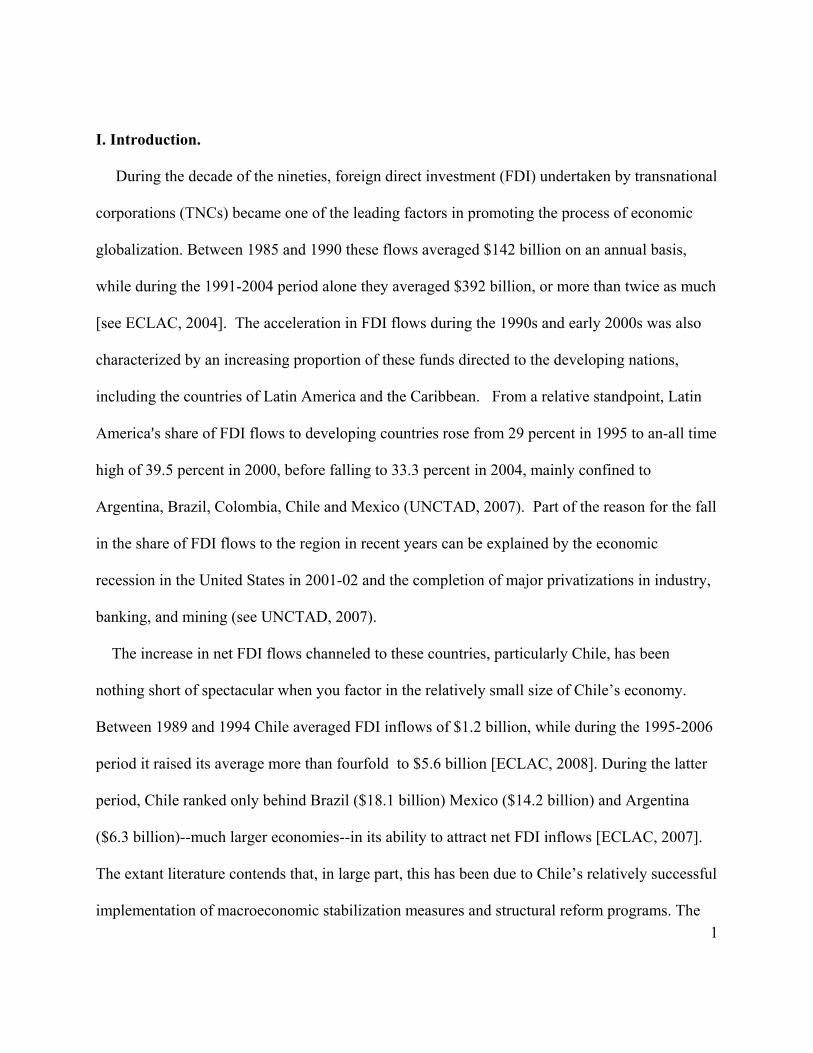
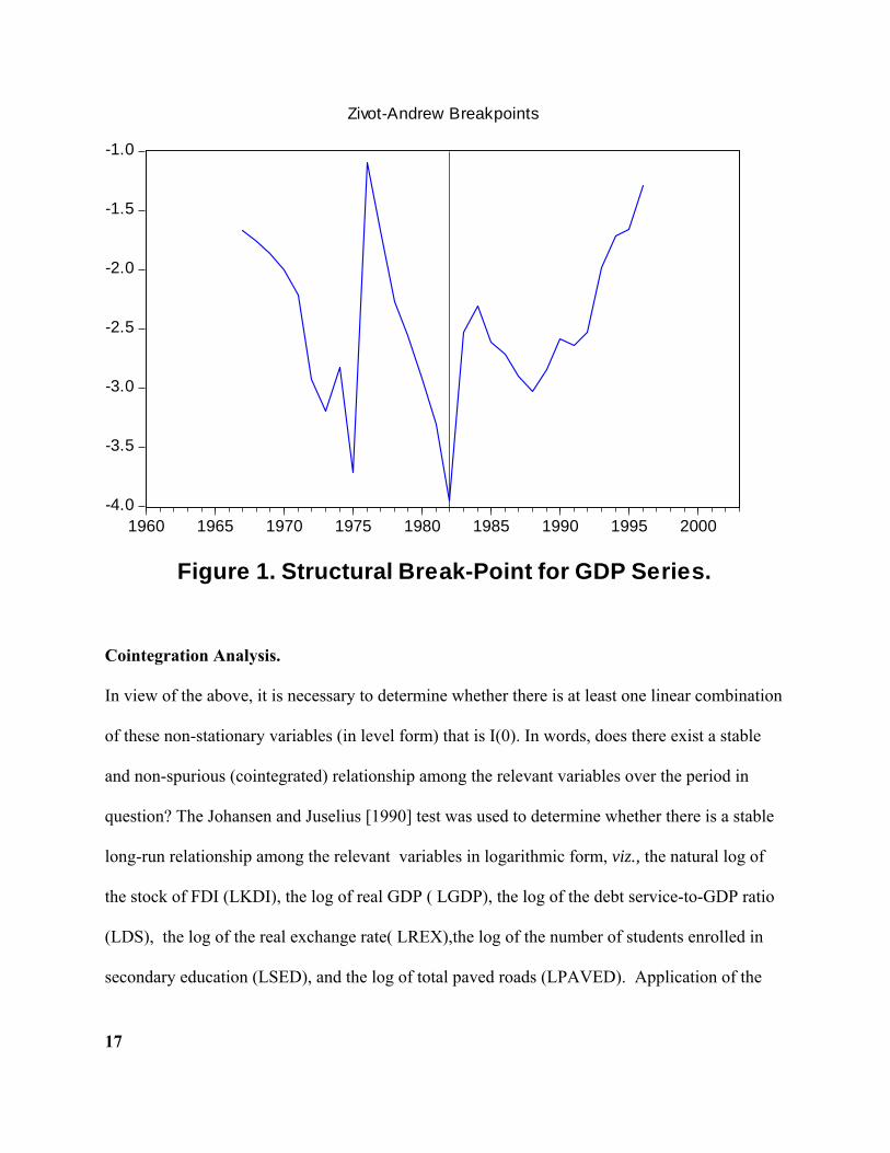
As can be readily seen, the estimates reported in Table 3 for the series in level form are

consistent with those in Table 2. For all of the series in question, Table 3 shows that the null

hypothesis with a structural break in both the intercept and the trend cannot be rejected at the 5

percent level of significance.vii In addition, the Z-A test identifies endogenously the single most

significant structural break in every time series. In view of space constraints, Figure 1 below

shows visually the endogenously determined break-date for the GDP series.viii

17

-4.0

-3.5

-3.0

-2.5

-2.0

-1.5

-1.0

1960 1965 1970 1975 1980 1985 1990 1995 2000

Zivot-Andrew Breakpoints

Figure 1. Structural Break-Point for GDP Series.

Cointegration Analysis.

In view of the above, it is necessary to determine whether there is at least one linear combination

of these non-stationary variables (in level form) that is I(0). In words, does there exist a stable

and non-spurious (cointegrated) relationship among the relevant variables over the period in

question? The Johansen and Juselius [1990] test was used to determine whether there is a stable

long-run relationship among the relevant variables in logarithmic form, viz., the natural log of

the stock of FDI (LKDI), the log of real GDP ( LGDP), the log of the debt service-to-GDP ratio

(LDS), the log of the real exchange rate( LREX),the log of the number of students enrolled in

secondary education (LSED), and the log of total paved roads (LPAVED). Application of the

18

likelihood ratio (L.R.) test showed that the null hypothesis of no cointegrating relationship can be

rejected at the 5 percent level (trace statistic = 81.91 > critical value = 76.97 (p-value: 0.02); and

Max-Eigen statistic= 30.63 > critical value = 27.58 (p-value: 0.0197)), thereby suggesting that

there is one unique linear combination of these non-stationary variables (in level form) that is

stationary.

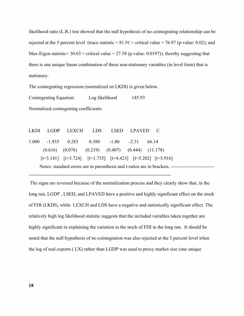
The cointegrating regression (normalized on LKDI) is given below.

Cointegrating Equation: Log likelihood 145.93

Normalized cointegrating coefficients:

LKDI LGDP LEXCH LDS LSED LPAVED C

1.000 -1.935 0.283 0.380 -1.80 -2.31 66.14

(0.616) (0.076) (0.219) (0.407) (0.444) (11.178)

[t=3.141] [t=3.724] [t=1.735] [t=4.423] [t=5.202] [t=5.916]

Notes: standard errors are in parenthesis and t-ratios are in brackets. ---------------------------

-----------------------------------------------------------------------------------------

The signs are reversed because of the normalization process and they clearly show that, in the

long run, LGDP , LSED, and LPAVED have a positive and highly significant effect on the stock

of FDI (LKDI), while LEXCH and LDS have a negative and statistically significant effect. The

relatively high log likelihood statistic suggests that the included variables taken together are

highly significant in explaining the variation in the stock of FDI in the long run. It should be

noted that the null hypothesis of no cointegration was also rejected at the 5 percent level when

the log of real exports ( LX) rather than LGDP was used to proxy market size (one unique

19

cointegrating vector was present), as well as with the inclusion of the dummy variables

(available upon request).ix

Results.

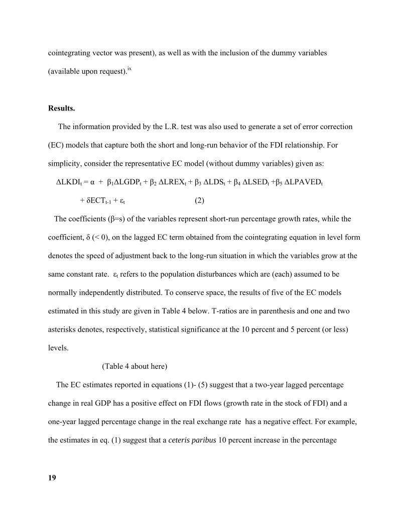
The information provided by the L.R. test was also used to generate a set of error correction

(EC) models that capture both the short and long-run behavior of the FDI relationship. For

simplicity, consider the representative EC model (without dummy variables) given as:

ΔLKDIt = α + β1ΔLGDPt + β2 ΔLREXt + β3 ΔLDSt + β4 ΔLSEDt +β5 ΔLPAVEDt

+ δECTt-1 + εt (2)

The coefficients (β=s) of the variables represent short-run percentage growth rates, while the

coefficient, δ (< 0), on the lagged EC term obtained from the cointegrating equation in level form

denotes the speed of adjustment back to the long-run situation in which the variables grow at the

same constant rate. εt refers to the population disturbances which are (each) assumed to be

normally independently distributed. To conserve space, the results of five of the EC models

estimated in this study are given in Table 4 below. T-ratios are in parenthesis and one and two

asterisks denotes, respectively, statistical significance at the 10 percent and 5 percent (or less)

levels.

(Table 4 about here)

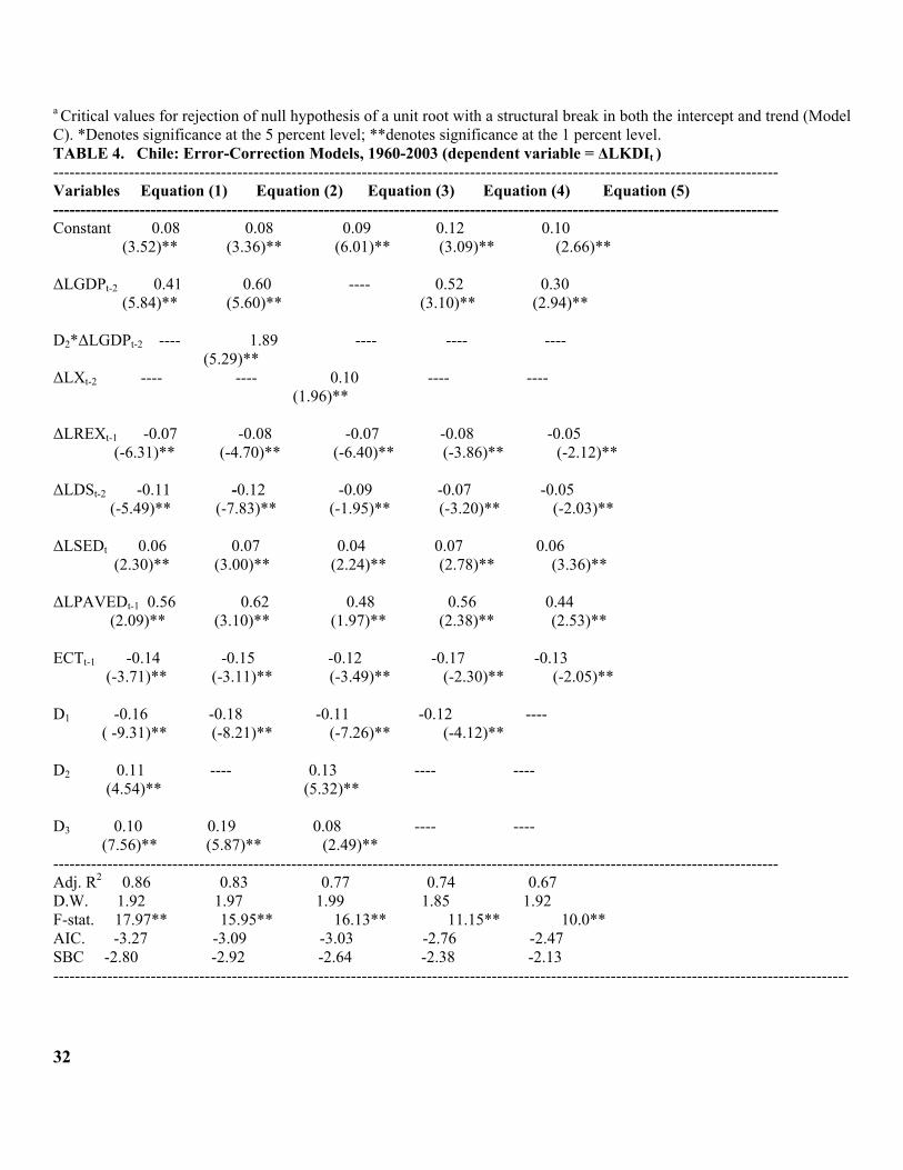
The EC estimates reported in equations (1)- (5) suggest that a two-year lagged percentage

change in real GDP has a positive effect on FDI flows (growth rate in the stock of FDI) and a

one-year lagged percentage change in the real exchange rate has a negative effect. For example,

the estimates in eq. (1) suggest that a ceteris paribus 10 percent increase in the percentage

20

growth rate in real GDP during the current period generates a 4.1 percent increase in FDI flows

to the country within two years, while a 10 percent rise in the growth rate in the real exchange

rate (a depreciation) during the current period generates a 0.7 percent reduction in FDI flows in

the following year. As anticipated, the ratio of debt service payments-to-exports variable had a

negative and statistically significant effect on FDI flows when lagged 2 periods, while the

education variable had a positive and significant effect. In the latter case, a 10 percent increase in

the growth rate of secondary enrollment during the current period generates a 0.6 percent

increase in FDI flows to the country. Finally, the relatively high and significant estimate for the

physical infrastructure variable suggests that it is highly important in attracting FDI flows to the

country. For example, an increase in the percentage growth rate of paved roads by 10 percent

generates, on average, a 5.6 percent increase in FDI flows to the country, ceteris paribus.x From

an institutional standpoint, the results suggest that debt-led growth of the early 1980s (D3) and

the liberalization of foreign investment rules during the 1987-97 (D2) period had a positive and

statistically significant effect on FDI flows to Chile, while political and economic turmoil (D1),

particularly during the Allende administration and the transition to democracy, had a negative

and statistically significant impact.

Although the real GDP variable is lagged in the reported EC models, it is possible that FDI

flows may affect real GDP. To test for this possibility I ran a Pairwise Granger Causality Test

with one and two lags. The results show that the null hypothesis that ΔLGDP does not “Granger

cause” ΔLKDI could be rejected at the 1 percent level for one lag (p-value: 0.003) and at the 5

percent level with two lags (p-value= .0198), while the hypothesis that ΔLKDI does not

“Granger cause” ΔLGDP could not be rejected (p-value: 0.588 for one lag, and for two

21

lags=0.803). Of course, this test says nothing about “causation” per se; it only provides

information about whether changes in one variable precede changes in another. The evidence

suggests that changes in GDP precede changes in FDI. Similarly, the results for the pairs ΔLKDI

and ΔLREX and ΔLKDI and ΔLPAVED suggest that changes in both LREX and LPAVED

precede changes in FDI for one lag. The estimates for two lags are consistent with the one lag

results and are statistically significant at the one percent level. Insofar as the ΔLKDI and ΔLSED

pair is concerned, the results are inconclusive for one lag, but in the case of two lags changes in

LSED precede changes in LKDI at the five percent level. Finally, the estimates are inconclusive

with respect to the pairs ΔLKDI and ΔLDS because, despite the fact that changes in DS precede

those in FDI for one lag, it is also the case that changes in FDI precede changes in DS (the nature

of the lags for the variables was determined via the Akaike-Schwarz criteria.)xi

The ECM model was also estimated with dummy variable D2 multiplied by the change in

the log of real GDP. By estimating this variable interactively with the change in the log of real

GDP one can assess whether the consolidation of market-oriented reforms had a positive and

significant effect on the capacity of market size to affect real FDI flows. The results are reported

in eq. (2). In general, the results are consistent with those of eq. (1), and the interactive term

suggests that the reforms enhanced further the impact of market size on FDI flows. Table 4 also

reports results for the basic ECM model without the dummy variables to determine whether the

quantitative variables maintain their signs and significance. As can be seen by eq. (5), the

estimates are robust to the exclusion of the qualitative variables , and the EC model retains a

relatively high degree of significance and explanatory power. Along the same lines, Eq. (4)

22

shows that the inclusion of qualitative variable D1 by itself does not alter the sign nor the

significance of the quantitative variables in the EC model.

Finally, for purposes of comparison, eq. (3) reports estimates that include the percentage

growth rate in real exports (ΔLX) as the relevant proxy for Chile=s potential market size. The

coefficient for the export variable in eq. (3) suggests that it is positive and highly significant

when lagged two periods, viz., a 10 percent increase in the growth rate of real exports during the

current period generates a 1percent increase in FDI flows to the country within two years. The

estimates for the other variables are not altered and the model retains a relatively high degree of

explanatory power. This variable was also estimated with an interactive term (not reported in

Table 3), and the reported estimate [1.91 (t-ratio=6.60)] is consistent with the estimate reported

in eq. (2) above, viz., the implementation of market-based outward-oriented reforms further

enhanced the positive (lagged) effect of export growth on FDI flows. These results are not

altogether surprising in view of the fact that the simple correlation between Chile=s real exports

and real GDP over the period in question is .945.xii

The Bruesch-Godfrey serial correlation LM test (with two lags) indicated that first order serial

correlation was present in the reported EC models, so they were corrected by including an AR(1)

term. The D.W. values for all equations in Table 4 suggest that the null hypothesis of no

(positive) first order autocorrelation cannot be rejected at the 5 percent level. The relative fit and

efficiency of the EC models is quite good for eqs. (1)-(3) and, as the theory predicts, the lagged

residual terms in all eqs. are negative and statistically significant; e.g., the lagged EC term in eq.

(1) suggests that a 10 percent deviation during the current period from long run FDI flows to

Chile is corrected by about 1.4 percent in the next year on average. Finally, stability tests were

23

conducted to determine whether the null hypothesis of no structural break could be rejected for

key periods in Chile=s history. The Chow breakpoint tests suggested that the null hypothesis

could not be rejected for the crises years 1973 (F-stat: 1.373; p-value: 0.265), 1975 (F-stat: 1.63;

p-value: 0.186), and 1982 (F-stat; 1.306; p-value: 0.291).

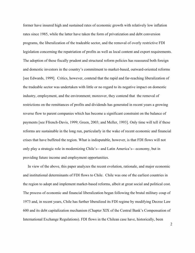
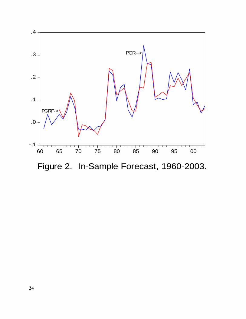
Before concluding, the EC models were used to track the historical data on the percentage

growth rate in inward FDI flows to Chile during the period under review. Figure 2 below,

corresponding to equation (1) in Table 4, shows that the model was able to track the turning

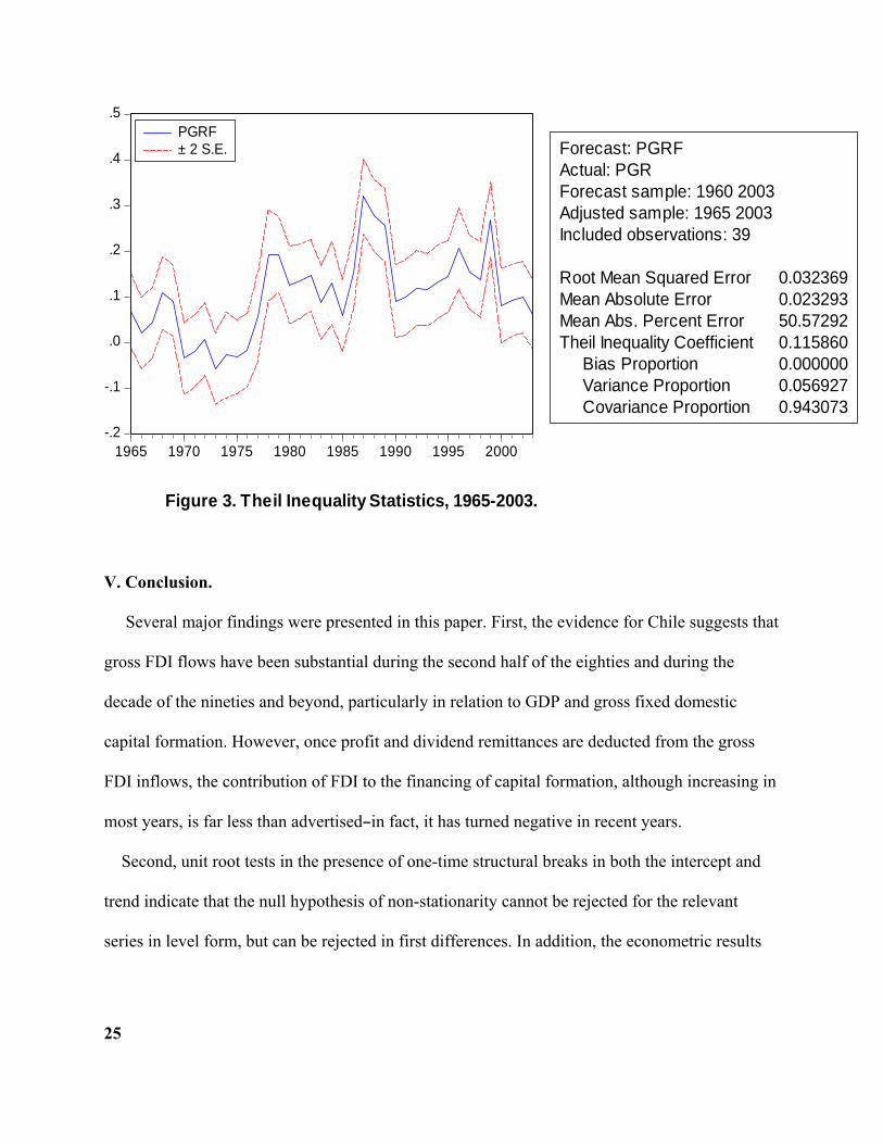
points in the actual series quite well. PGR) refers to the actual series and (PGRF) denotes the in-

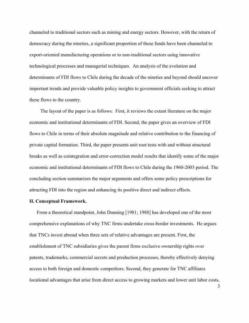
sample forecast. In addition, Figure 3 shows that the Theil inequality coefficient for this model

is 0 .115, which is well below the threshold value of 0.3, and suggests that the predictive power

of the model is quite good [see Theil, 1966]. The Theil coefficients can be decomposed into three

major components: the bias, variance, and covariance terms. Ideally, the bias and variance

components should equal zero, while the covariance proportion should equal one. The estimates

reported in Figure 3 suggest that all of these ratios are close to their optimum values (bias= 0.00,

variance= 0.05, and covariance = 0.94). Sensitivity analysis on the coefficients also revealed that

changes in the initial or ending period did not alter the predictive power of the selected models

(results are available upon request).

24

-.1

.0

.1

.2

.3

.4

60 65 70 75 80 85 90 95 00

Figure 2. In-Sample Forecast, 1960-2003.

PGRF->

PGR-->

25

-.2

-.1

.0

.1

.2

.3

.4

.5

1965 1970 1975 1980 1985 1990 1995 2000

PGRF± 2 S.E. Forecast: PGRF

Actual: PGRForecast sample: 1960 2003Adjusted sample: 1965 2003Included observations: 39

Root Mean Squared Error 0.032369Mean Absolute Error 0.023293Mean Abs. Percent Error 50.57292Theil Inequality Coefficient 0.115860 Bias Proportion 0.000000 Variance Proportion 0.056927 Covariance Proportion 0.943073

Figure 3. Theil Inequality Statistics, 1965-2003.

V. Conclusion.

Several major findings were presented in this paper. First, the evidence for Chile suggests that

gross FDI flows have been substantial during the second half of the eighties and during the

decade of the nineties and beyond, particularly in relation to GDP and gross fixed domestic

capital formation. However, once profit and dividend remittances are deducted from the gross

FDI inflows, the contribution of FDI to the financing of capital formation, although increasing in

most years, is far less than advertisedBin fact, it has turned negative in recent years.

Second, unit root tests in the presence of one-time structural breaks in both the intercept and

trend indicate that the null hypothesis of non-stationarity cannot be rejected for the relevant

series in level form, but can be rejected in first differences. In addition, the econometric results

26

suggest that market size (proxied by either real GDP or real exports), the real exchange rate, the

debt-service ratio, the human capital variable, and the physical infrastructure variable had their

anticipated signs and were statistically and economically significant in explaining the variation

of FDI flows to Chile over the 1960-2003 period. In addition the institutional variables, captured

by the included dummy variables, had their expected effects and were statistically significant. In

particular, the interactive term suggests that institutional reforms have enhanced the effect of

traditional variables such as real GDP or real exports in attracting FDI flows to the nation.

Third, the Johansen cointegration test indicated that there is a stable relationship among the

relevant variables in level form which keeps them in proportion to one another over the long run.

This is a highly important contribution to the extant literature because previous econometric

studies relating to Chile have failed to determine whether the estimated relationships were

spurious or not. Finally, the EC models reported in Table 4 suggests that short-run deviations

from the long-run FDI relationship are corrected in subsequent periods and, equally as important,

Figure 1 shows that the in-sample forecasts of the EC models are able to track the turning points

in the data relatively well.

From a research and policy standpoint, it would be highly important for future investigators to

determine whether the massive inflows of FDI the country has received in recent years have been

directed to “greenfield” sectors where positive direct and indirect effects in the form of

“intangibles” such as the transfer of technology and managerial knowhow are likely to be present

(see endnote 1). If econometric evidence shows that inflows directed to these sectors have had a

positive and economically significant effect on labor productivity growth, then it may help offset

the short-term costs associated with generous subsidies, tax concessions, and pressures on the

27

balance of payments as a result of the substantial growth in TNCs’ remittances of profits and

dividends from the country in recent years. The estimates also suggest that FDI flows will be

attracted, on a long-term basis, to developing countries such as Chile provided that policy makers

avoid sharp depreciations of the real exchange rate that lower the real (dollar) rate of return on

FDI investments and implement policies that ensure the availability of a well-educated citizenry

and adequate physical infrastructure.

REFERENCES Agosin, Manuel R., ed. 1995. Foreign Direct Investment in Latin America. Washington, D.C.:

Inter-American Development Bank. Bloomstrom, M. And E. Wolff. Multinational Corporations and Productivity Convergence

in Mexico. 1994. In Convergence of Productivity: Cross-National Studies and Historical Evidence, edited by W. Baumol, R. Nelson, and E. Wolff. Oxford: Oxford University Press. Bouton, Lawrence and Mariusz A. Sumlinski. 1999. Trends in Private Investment in Developing

Nations: Statistics for 1970-98. Washington, D.C. : International Finance Corporation. Cypher, James M. And James L. Dietz. 2003 The Process of Economic Development. New York:

Routledge. De Mello, Jr. Luiz R. 1997. AForeign Direct Investment in Developing Countries and Growth: A

Selective Survey.@ Journal of Development Studies, 34, 1 (October): 1-34. De Vita, Glauco and Kevin Lawler. 2004. AForeign Direct Investment and its Determinants: A

Look to the Past, A View to the Future.@ In Foreign Investment in Developing Nations, edited by H.S. Kehal. New York: Palgrave Macmillan, Ltd. Dickey, D., and W. Fuller, 1979. ALikelihood Ratio Statistics for Autoregressive Time Series

with a Unit Root.@ Econometrica, June: 1057-1072. ECLAC. 2005. Foreign Investment in Latin America and the Caribbean, 2004 Report. Santiago, Chile: United Nations.

28

ECLAC. 2007. Foreign Investment in Latin America and the Caribbean, 2006 Report. Santiago,

Chile: United Nations. ECLAC. 2008. Foreign Investment in Latin America and the Caribbean, 2007 Report. Santiago, Chile: United Nations. ECLAC. 1998. La Inversion Extranjera en America Latina y El Caribe. Santiago, Chile: United

Nations. Edwards, S. 1999. AHow Effective are Capital Controls?@ Journal of Economic Perspectives, 13, 4(Fall): 65-84. Engle, R.F. and C.W.J. Granger. 1987. ACointegration and Error Correction: Representation,

Estimation, and Testing.@ Econometrica 55 (March): 251-76. Figueroa, Adolfo. 1998. Equity, Foreign Investment and International Competitiveness in Latin

America. The Quarterly Review of Economics and Finance, Fall, 391-408. Ffrench-Davis, R. and Munoz, O. 1992. AEconomic and Political Instability in Chile,@ in Simon

Teitel, ed., Towards a New Development Strategy for Latin America. Washington, DC: Inter-American Development Bank. Ffrench-Davis, R. and M.R. Agosin. 1999. ACapital Flows in Chile: From the Tequila to the

Asian Crises@ Journal of International Development, 11: 121-139. Green, Duncan. 2003. Silent Revolution: The Rise and Crisis of Market Economies in Latin

America. New York: Monthly Review Press. Hoffman, Andre A. 2000. The Economic Development of Latin America in the Twentieth

Century. MA.: Northhampton. Johansen, Soren and K. Juselius. 1990. AMaximum Likelihood Estimation and Inference on

Cointegration with Applications to the Demand for Money.@ Oxford Bulletin of Economics and Statistics, 52 (May): 169-210. Lee, J. and M.C. Strazicich. 2003. “Minimum Lagrange Multiplier Unit Root Test with Two Structural Breaks,” The Review of Economics and Statistics, 85 (4), 1082-1089. OECD. 2003. Economic Surveys: Chile. Paris: OECD. Perron, P. 1989. “The Great Crash, the Oil Price Shock and the Unit Root Hypothesis,” Econometrica, 57, 1361-1401.

29

Plasschaert, S. ed. 1994. Transnational Corporations: Transfer Pricing and Taxation. London: Routledge.

Ramirez, Miguel D. 2000. AForeign Direct Investment in Mexico: A Cointegration Analysis.@

The Journal of Development Studies, 37 (October): 138-162. Ros, Jaime. Financial Markets and Capital Flows in Mexico. In Foreign Capital in Latin

America, edited by Jose A. Ocampo and Roberto Steiner. Washington, D.C.: Inter-American Development Bank, 1994. Theil, H. 1966. Applied Economic Forecasting. Amsterdam: North-Holland. United Nations. 2007. World Investment Report 2007: Trends and Determinants. Switzerland:

United Nations. Waheed, M.A., A. Tasneem, and G.S. Pervaiz. 2007. “Structural Breaks and Unit Roots: Evidence From Pakistani Macroeconomic Time Series,” MPRA Paper, No. 1797, November, 1-18. Zhang, Kevin H. 2001. “What Attracts Foreign Multinational Corporations to China?” Contemporary Economic Policy, July, 336-346. Zivot, E. and D. Andrews. 1992. “Further Evidence of Great Crash, the Oil Price Shock, and Unit Root Hypothesis,” Journal of Business and Economic Statistics, 10, 251-270.

30

TABLE 1 Part A. Chile: FDI Flows as a Percentage of Gross Fixed Capital Formation, 1990-2005 ---------------------------------------------------------------------------------------------------------------------------------------- 1990 1991 1992 1993 1994 1995 1996 1997 1998 1999 2000 2001 2002 2003 2004 2005 ---------------------------------------------------------------------------------------------------------------------------------------- 8.3 7.2 7.5 7.2 14.6 12.1 25.7 27.9 22.9 54.31 22.0 17.1 15.4 16.1 34.6 27.4 ---------------------------------------------------------------------------------------------------------------------------------------- Part B. Chile: FDI Flows adjusted for the Remittance of Profits and Dividends as a Percentage of Gross Fixed Capital Formation, 1990-2005.2 ------------------------------------------------------------------------------------------------------------------------------------------ 1990 1991 1992 1993 1994 1995 1996 1997 1998 1999 2000 2001 2002 2003 2004 2005 ------------------------------------------------------------------------------------------------------------------------------------------ 4.8 -1.7 -2.1 0.8 6.0 10.9 16.7 17.4 17.8 43.8 8.1 2.1 - 0.6 -13.3 -7.6 -9.3 ------------------------------------------------------------------------------------------------------------------------------------------ Source: United Nations, World Investment Report, 2007. New York: United Nations, 2007; and ECLAC, Statistical Yearbook for Latin America and the Caribbean, 2006. Santiago, Chile: United Nations, 2006, Table 2.1.1.54, p. 132, and Table 2.1.1.57, p. 135. 1The unusually high figure for Chile is the coincidental result of a doubling of FDI inflows and a steep drop in gross fixed capital formation in 1999. 2A negative value indicates that profits and dividend payments exceeded FDI inflows for that year, thereby diverting resources away from fixed capital formation.

31

TABLE 2. Conventional Unit Root Tests for Stationarity, Sample Period 1960-2003. Variables Levels First Difference 5% Critical Valuea 1% Critical Value ---------------------------------------------------------------------------------------------------------------------------------------- LKDI 0.91 -3.05* -2.94 -3.59 LGDP 0.21 -4.05** -2.94 -3.59 LREX -1.23 -4.55** -2.94 -3.59 LX 0.34 -7.20** -2.94 -3.59 LDS -2.64 -6.86** -2.94 -3.59 LSED -1.07 -3.91** -2.94 -3.59 LPAVED -2.68 -4.12** -2.94 -3.59 LRPAVED -2.47 -4.51** -2.94 -3.59 ----------------------------------------------------------------------------------------------------------------------------------------- aMackinnon critical values for rejection of null hypothesis of a unit root under the assumption of a stochastic trend. *Denotes significance at the 5 percent level; **denotes significance at the 1 percent level. TABLE 3. Zivot-Andrews One-break Unit Root Test, Sample Period 1960-2003. Variables Levels Break Year 5% Critical Valuea 1% Critical Value ---------------------------------------------------------------------------------------------------------------------------------------- LKDI -4.32 1980 -5.08 -5.57 LGDP -3.95 1982 -5.08 -5.57 LREX -3.91 1985 -5.08 -5.57 LX -4.48 1973 -5.08 -5.57 LDS -3.93 1975 -5.08 -5.57 LSED -4.41 1971 -5.08 -5.57 LPAVED -5.07 1992 -5.08 -5.57 LRPAVED -4.77 1992 -5.08 -5.57 -----------------------------------------------------------------------------------------------------------------------------------------

32

a Critical values for rejection of null hypothesis of a unit root with a structural break in both the intercept and trend (Model C). *Denotes significance at the 5 percent level; **denotes significance at the 1 percent level. TABLE 4. Chile: Error-Correction Models, 1960-2003 (dependent variable = ΔLKDIt ) -------------------------------------------------------------------------------------------------------------------------------------- Variables Equation (1) Equation (2) Equation (3) Equation (4) Equation (5) -------------------------------------------------------------------------------------------------------------------------------------- Constant 0.08 0.08 0.09 0.12 0.10 (3.52)** (3.36)** (6.01)** (3.09)** (2.66)** ΔLGDPt-2 0.41 0.60 ---- 0.52 0.30 (5.84)** (5.60)** (3.10)** (2.94)** D2*ΔLGDPt-2 ---- 1.89 ---- ---- ---- (5.29)** ΔLXt-2 ---- ---- 0.10 ---- ---- (1.96)** ΔLREXt-1 -0.07 -0.08 -0.07 -0.08 -0.05 (-6.31)** (-4.70)** (-6.40)** (-3.86)** (-2.12)** ΔLDSt-2 -0.11 -0.12 -0.09 -0.07 -0.05 (-5.49)** (-7.83)** (-1.95)** (-3.20)** (-2.03)** ΔLSEDt 0.06 0.07 0.04 0.07 0.06 (2.30)** (3.00)** (2.24)** (2.78)** (3.36)** ΔLPAVEDt-1 0.56 0.62 0.48 0.56 0.44 (2.09)** (3.10)** (1.97)** (2.38)** (2.53)** ECTt-1 -0.14 -0.15 -0.12 -0.17 -0.13 (-3.71)** (-3.11)** (-3.49)** (-2.30)** (-2.05)** D1 -0.16 -0.18 -0.11 -0.12 ---- ( -9.31)** (-8.21)** (-7.26)** (-4.12)** D2 0.11 ---- 0.13 ---- ---- (4.54)** (5.32)** D3 0.10 0.19 0.08 ---- ---- (7.56)** (5.87)** (2.49)** -------------------------------------------------------------------------------------------------------------------------------------- Adj. R2 0.86 0.83 0.77 0.74 0.67 D.W. 1.92 1.97 1.99 1.85 1.92 F-stat. 17.97** 15.95** 16.13** 11.15** 10.0** AIC. -3.27 -3.09 -3.03 -2.76 -2.47 SBC -2.80 -2.92 -2.64 -2.38 -2.13 ---------------------------------------------------------------------------------------------------------------------------------------------------

33

Terms in parentheses are t-ratios. *Significant at the 10% level; **significant at the 5% level. ECT= Error-Correction Term; AIC = Akaike Information Criterion; SBC Schwartz Bayesian Criterion.

NOTES

1. FDI flows channeled through both Chapter XIX and DL 600 during the 1987-95 period were primarily confined to the mining sector and traditional industries such as textiles, leather, and footwear where the country=s has a comparative advantage based on low unit labor costs and natural resources. However, during the 1996-2002 period there was a marked decline in the proportion of FDI channeled to the mining sector and a concomitant increase in the share allocated to so-called Agreenfield@ sectors such as telecommunications, manufacturing, energy, and financial services [see ECLAC, 2003]. This trend has also been accompanied by a change in the geographic origin of capital flows away from United States and Canadian firms and towards European (particularly Spanish) companies in the service (finance and telecommunications) sector.

2. Agosin [1995, pp. 121-122] estimates a simple regression model that tries to explain the variation in FDI flows to Chile during the 1975-93 period. He finds that both the level of real GDP in constant dollars and the real depreciation of the exchange have a positive and statistically significant effect on FDI flows. He also includes a dummy variable to capture the adoption of the debt conversion program (Chapter XIX), and finds that it also has a positive and statistically significant impact on FDI flows. The major problem with this otherwise interesting paper is that the author does not undertake a cointegration analysis of the FDI investment relationship. Given the likely presence of unit roots in the level data, the reported estimates are not reliable.

3. It would be preferable to use a more direct measure of costs such as unitary labor costs. Unfortunately, data on Chilean unit labor costs for the period under review (going as far back as the sixties and early seventies) is not available in a consistent and reliable form.

4. Investment data was cross-checked with that found in the International Finance Corporation, Trends in Private Investment in Developing Countries: Statistics for 1970-98 [1999] and no significant differences were discerned.

5. There are no initial estimates for the foreign capital stock in Chile in 1960 or, for that matter, its rate of depreciation. This study constructed the stock of foreign capital in Chile based on the assumption that its general trend does not differ significantly from that of the country=s total fixed private capital stock. The capital growth rate and depreciation estimates were obtained from Hoffman (2000, Appendix H, p. 277). The initial private capital stock is constructed on an assumed private capital stock growth rate of 3 percent (equal to the growth rate of GDP in 1940-60) and the following estimates for depreciation: 2.5 percent for construction (40 years of service life) and 7 percent for machinery and equipment (14 years). In view of the fact that there are no disaggregated data on the composition of foreign capital flows to Chile for the period under review (viz., structures vs. machinery and equipment), this study used a 5 percent depreciation rate (20 years of service life). The latter figure is the same as that used by ECLAC (1998) in its computation of capital stocks for several major Latin American nations (including Chile, see Technical Note 2, pp. 162-165). In fact, ECLAC argues that the higher rate of depreciation is more appropriate in view of the faster obsolescence rate for machinery and equipment with a high technological content. For example, ECLAC reports that at the beginning of the 1990s computers and related equipment were

34

depreciated in 5 years, yet by the end of the decade, they were depreciated in just two years (p. 163). Finally, Hoffman reports that the capital-output ratio for Chile was quite stable for the 1950-60 period, averaging 2.74, and for the 1957-60 period used in this study, it was unchanged at 2.7 (for further details, see Appendix H, pp. 276-278). To ensure the robustness of the econometric results, other estimates of the rate of depreciation were used (1 and 10 percent) , as well as different estimates of the initial foreign capital stock (e.g., summing over 3 and 5 years), but the results were not altered significantly.

6. Unit root tests under the assumption of a deterministic trend also indicated that in level form the variables were non-stationary. Thus, the common practice of de-trending the data would not render them stationary (results are available upon written request).

7. The Z-A one-break point unit root test was also performed for the relevant time series in differenced form under the assumption of model C and the null hypothesis was rejected at the 5 percent level or lower in all cases. 8. The analysis undertaken in this study only tests for the presence of a single endogenously determined structural break. In a recent paper, Lee and Stazicich (2003) show that when there are, in fact, two structural breaks in the data, assuming erroneously that there is only one can result in a loss of power of the test. 9. I also performed an augmented (one lag) Dickey-Fuller (D-F) test on the residuals of the foreign investment function given in equation (3), Table 4 to determine if they were stationary. (The length of the lag was determined via the Akaike-Schwarz criterion.) The results (available upon request) indicated that the absolute value of the D-F stat. (3.997) was greater than the absolute value of the critical Mackinnon value at the 1 percent level (3.61), thereby rejecting the presence of a non-stationary process (a so-called unit root). Admittedly, this somewhat dated test for stationarity is consistent with the more robust L.R. ratio test reported in the paper. 10. The ECM model was also estimated with the growth rate in the percentage of paved roads and the results indicated that a ceteris paribus increase in the growth rate in the percentage of paved roads by 10 percent generates a 3.5 percent increase in FDI inflows (t-stat=2.00, p-value=.052). 11.The length of the lags is likely to change as the legal-institutional environment for conducting business in Chile improves. In this scenario, the flow of FDI to Chile is likely to become more responsive to any future changes in GDP and/or the real exchange rate, ceteris paribus.

12. I also estimated the EC model by including the growth rate in high income OECD countries (Europe, U.S. and Japan) as a proxy for market size in view of the fact that, in recent years, at least 60 percent of Chilean exports are destined to high income OECD nations (70 percent if China is included; see Banco de Chile, February 2004). However, GDP data for high income OECD countries was available only from 1970 onwards, so I had to use U.S. GDP data as a proxy for the 1960-69 period. This is not very problematic because during the 1960s the U.S. market absorbed close to 40 percent of Chilean exports (see Banco de Chile, Indicadores Economicos y Sociales, 1960-1988). Again, the ECM results remained basically the same and are available upon written request.