Trickle-Down Education? Effects of Public Colleges onPrimary and Secondary Education Markets in India∗

Maulik Jagnani†

Gaurav Khanna‡

This version: October 20, 2017

Please do not circulate without permission

Abstract

In this paper, we present the first estimates of the economic effects of colleges in low-income countries. Using multiple datasets, and a combination of event study anddifference-in-differences research designs, we study the effects of elite public colleges onprimary and secondary schooling markets in India. We find that elite public colleges ledto an increase in educational attainment, driven by children staying in school longer.These gains in attainment correspond with a larger role played by private schools asmore for-profit schools enter regions with new elite colleges, and students switch frompublic to private schools. We provide suggestive evidence that these effects on schoolingmarkets are driven by focal investments in water and electricity services, which reducesetup costs for private schools, and consequently, travel costs for school-age children.

JEL Codes: H52, I23, I25, O53Keywords: education markets, public colleges, enrollment, private schools, school choice, publicinfrastructure

∗We thank Wilima Wadhwa and Sam Asher for generously sharing data. We would like to thank Achyuta Adhvaryu, SamAsher, Chris Barrett, Arnab Basu, Jim Berry, Austin Davis, Maria Fitzpatrick, Teevrat Garg, Lakshmi Iyer, David Jaume,Ravi Kanbur, Margaret Lay, Shanjun Li, Claire Lim, Katherine Lim, Annemie Maertens, Doug Miller, Vesall Nourani, EswarPrasad and Kibrom Tafere for helpful comments. Kyongmo Do provided excellent research assistance. Seminar participantsat Cornell University, 2016 Annual Conference at the Indian Statistical Institute, Delhi, and 2017 Empirics and Methods inEconomics Conference at the University of Chicago provided useful feedback. Earlier version of this paper was circulated as“Unintended Effects of Public Colleges on Primary and Secondary Education Markets in India”.†Charles H. Dyson School of Applied Economics and Management, Cornell University. E: mvj22@cornell.edu‡School of Global Policy and Strategy, University of California, San Diego. E: gakhanna@ucsd.edu

1 Introduction

In India, some observers have criticized public investment in higher education as inordinate,

relative to the entire education budget, and expenditure on college infrastructure is perceived

to come at the expense of schooling infrastructure.1 By squarely pitting public investment

on colleges against public spending on schools, these normative observations presume an

understanding of the economic effects of both schools and colleges. However, although

schooling infrastructure has been shown to have large economic benefits in poor countries

(e.g., Birdsall, 1985; Duflo, 2001; Lavy, 1996; Lillard and Willis, 1994), as far as we know,

the effects of colleges in low-income countries have not been evaluated.2 This paper tries

to make progress on this issue by examining the effects of public colleges on the rest of the

local market for education – primary, middle and secondary schooling. We present the first

estimates of this relationship, study the various channels that determine these consequences,

and interpret our results through the lens of the literature on determinants of private schools,

school choice and educational attainment in low-income countries.

To measure the causal effect of public colleges on primary and secondary education

markets and understand the underlying mechanisms, we exploit the staggered roll-out, in-

stitutional features, and location guidelines, of elite public colleges setup in India between

2004-2014. Elite public colleges are institutions that are conferred a status of an ‘Institute

of National Importance’ by an act of the parliament, and receive special recognition and

funding from the federal government. Apart from the ‘elite’ nature of these institutions,

two other features distinguish them from ‘regular’ colleges or universities in India. First,

location of newer elite colleges has been a function of addressing regional imbalance caused

by the location of older such institutions. Second, student admissions into these colleges are

determined by extremely competitive nation-wide entrance tests. So, location or timing of

establishment is unlikely to be correlated with anticipated changes in local schooling mar-

kets. In our analysis, we restrict the sample to only those districts that eventually get an

elite public college. Thus, our identifying assumption is that the year of establishment is

1See for instance: Hiremath and Komalesha, 2017; Shah, 2017; Staff, 2011; Suri, 20172Colleges have been shown to have large economic benefits in advanced economies (e.g., Aghion et al., 2009; Cantoni and

Yuchtman, 2014; Kantor and Whalley, 2014).

1

exogenous to observables or unobservables that change over time, and are correlated with

the local schooling market.

We find three key results: First, we find that the establishment of a new elite public

college increased educational attainment amongst school-age children by 0.3 years at the

district level. Second, we show that elite public colleges increase the probability of private

school enrollment by over 5 percentage points (25%) in the short-run (year 1), and by over

10 percentage points (40%) in the medium term (year 3), and a substantial, corresponding

decrease in the probability of enrollment in public schools. Third, we examine the impacts

on the entry and exit of schools. Elite public colleges increase the number of private schools

by over 20% at the district level, but have no impact on the number of public schools.

We find suggestive evidence that these results are driven by focal investments in public

infrastructure. First, using satellite-measured nighttime lights as a proxy for electrification,

we show that an increase in proximity of an elite colleges led to a large increase in the density

of nighttime lights – villages located within 10 km from the new college saw an increase of

over 15% in nighttime luminosity. Relatedly, villages in districts that get a public college

are 18 percentage points more likely to have access to electricity for agricultural use and 6

percentage points more likely to have access to tap water. Such investment in water and

electricity services can reduce setup costs for private schools. Furthermore, conditional on

availability of public schooling infrastructure, entry of private schools could potentially solve

a (travel) cost constraint for the marginal child enabling her to get more years of education.

Indeed, we find that amongst the districts that received a public college, districts that were

relatively underserved by government schools saw a larger increase in the number of private

schools, a larger increase in the probability of private school enrollment, and correspondingly,

a larger decrease in public school enrollment. Furthermore, gains in educational attainment

were concentrated in these regions.

In investigating how elite public colleges affect schooling markets, this paper contributes

to three literatures. First, we contribute to the literature examining the economic effects of

infrastructure in developing countries (e.g., Adukia, Asher and Novosad, 2016; Burlig and

Preonas, 2016; Donaldson, 2017; Duflo and Pande, 2007; Lipscomb, Mobarak and Barham,

2011). Few of these studies have also examined the effects of infrastructure on human

2

capital. Importantly, there also exists a large literature evaluating the effects of schooling

infrastructure on educational outcomes (e.g., Duflo, 2001; Khanna, 2015). In this paper,

we present the first estimates of the development impacts of college infrastructure, and

specifically, the effects of colleges on local schooling markets. Relatedly, we also contribute

to the literature investigating externalities of government spending in the developed world

(e.g., Kline and Moretti, 2014; Serrato and Wingender, 2016). Our back-of-the-envelope

estimates suggest that indirect benefits through primary and secondary education markets

are at least 48% of the direct benefits of elite public colleges incurred through training

undergraduate and graduate students.

The second is the literature of the determinants of private provision of education in low-

income countries (e.g., Andrabi, Das and Khwaja, 2013; Kremer and Muralidharan, 2008).

We find suggestive evidence that elite colleges crowd-in investments in public infrastructure,

likely facilitating entry of private schools by reducing setup costs. Pal (2010) has also shown

that access to village infrastructural facilities is correlated with a higher likelihood of having

a private school in the community. Public schools are less likely to respond to such ad-

vancements since in centralized education systems, government resources may be allocated

to regions that are underserved (Duflo, 2001; Kremer and Muralidharan, 2008).

Third, our paper relates to the larger literature on educational attainment (Burde and

Linden, 2013; Duflo, 2001; Muralidharan and Prakash, 2017; Oster and Millett, 2013), and

the related literature on school choice, in low-income countries (Alderman, Orazem and

Paterno, 2001; Carneiro et al., 2016; Carneiro, Das and Reis, 2015). We find that the effects

on private school enrollment and educational attainment are larger in regions with fewer

public schools. This suggests that transportation costs may be an important determinant of

school choice, and can also affect educational attainment. Interestingly, Alderman, Orazem

and Paterno (2001) too finds that lowering distance increase enrollment in private schools in

Pakistan, partly by transfers from public schools. While, Muralidharan and Prakash (2017)

show that providing girls with bicycle in India led to an increase in educational attainment

by reducing the time and safety cost of school attendance.

The rest of the paper is organized as follows. In Section 2 we provide a model of school

choice and private school entry. Section 3 gives background information on elite public

3

colleges in India, and Section 4 describes the data. In Section 5 we investigate the impacts

of elite public colleges on educational attainment, enrollment in both state-run and private

schools, and number of primary and secondary schools. We discuss potential mechanisms

behind these empirical patterns in Section 6, and Section 7 concludes.

2 A Model of School Choice & Private School Entry

2.1 Supply of Private Schools

The supply of state-run or public schoolsN0 in district d is determined exogenously by district

administrators. The supply of private schools, on the other hand, is market determined; they

enter if they can earn positive profits.3

Private schools are profit maximizers and have heterogeneous costs.4 They are also price

takers in a competitive market and charge a fee p. Muralidharan and Sundararaman (2015)

find that children enrolled in private schools do not perform better than their peers in public

schools on subjects that are taught in both schools, although private schools are more cost-

effective. In our model, private schools have the same output as public schools, although the

operating costs might be different; and we have heterogeneity in efficiency amongst private

schools (Kremer and Muralidharan, 2008).

We begin by looking at the profit function of school j in district d with inputs Xj. We

define total educational output (in student-years) as Qj = θXj and cost function Z(Xj) =

z1jXj + 12z2X

2j to be quadratic.5 θ is the average education level in the district and captures

demand externalities driven by aspirations and peer effects (Birdsall, 1982; Bobonis and

Finan, 2009). For instance, proximity to an elite public college may increase the demand for

schooling. z1j reflects the heterogeneity in costs across schools and districts, drawn from the

distribution G(z1j), where some schools use their inputs more effectively than others. This

distribution varies across regions d as it may be cheaper to hire teachers in some districts,

3For notational convenience we drop the district sub-script d from our equations, even though quantities vary across districts.4Alternatively, they could have been modeled as having heterogeneous productivities, with the same result.5While easy to hire the first few teachers/administrators, it is more costly to hire the next as the pool of candidates dwindles.

4

while others may have better public infrastructure like electricity or drinking water.

πj = Qjp− Z(Xj) = pθXj − Z(Xj)

Implying X∗j =pθ − z1j

z2

, output is Q∗j = θpθ − z1j

z2

, and profit function π∗j =(pθ−z1j)2

2z2.

The total number of potential private schools is N . School j would enter only if its

profit is positive, and cost z1j is drawn from G(z1j). The fraction of schools in the district

is G(pθ), and the number of private schools in the district that enter is

N1 = N

∫ pθ

0

z1j dG(z1j) = pθN

Given this, the total supply of schooling in the district is

QSy =

N1∑j=1

Qj =

N1∑j=1

θpθ − z1j

z2

=pθ

2N

z2

(pθ − z1) (1)

2.2 Demand for Schooling and School Choice

Demand for schooling depends on the costs of going to school and the returns to schooling.

Costs vary across individuals based on criteria like tuition, distance to the nearest school(s),

ability and wealth. The cost for child i to attend school j is

cij = αpk + βTij − γln(Wi)−∆i (2)

Tuition is pk, travel costs Tij, wealth Wi, and ability ∆i. The tuition pk = 0 for public

schools, and pk = p for private schools. Increase in wealth makes schooling more affordable,

allowing us to capture the “consumption value” of education. Household wealth Wi, travel

costs Tij and abilities ∆i have distributions where the mean of the distributions (ln(w), δ

and Tk) vary across districts:

ln(Wi) = ln(w) + ζi & ∆i = δ + δi & Tij = Tk + ηij for{k = s, p}

For ease of notation, we define an error term εij based on these costs, and restate the cost

5

function cij:

εij ≡ βηij − γζi − δi & cij = αpk + βTk − γln(w)− δ + εij for {k = s, p}

Children will only attend school if the returns to education, r, are greater than the cost

of attending school. If a child decides to attend school, the choice of the school only depends

on cost, where school J is chosen if:

qi = 1(r −min(cij) > 0) = 1(r −min(αpk + βTk − εij) + γln(w) + δ > 0) (3)

with the returns to education r being similar across both public and private schools.6

The probability of a student going to school k depends on whether school k is public or

private. There are N0 public schools and N1 private schools. If the costs εij is i.i.d. with

distribution F(.), the aggregate demand for private school is

Qp = MN1F (φ− αp)[1− F (φ)]N0 [1− F (φ− αp)]N1−1 , (4)

where where φ ≡ r − βTk + γln(w) + δ. Notice from the supply-side N1 = Npθ.

2.3 Equilibrium

In equilibrium the supply and demand of private schooling are equal, allowing us to equate

Equations (1) and (4).

MN1F (φ− αp)[1− F (φ)]N0 [1− F (φ− αp)]N1−1 =N1θ

z2

(pθ − z1

)(5)

In order to solve for a closed form solution and do comparative statics we specify the

error term distribution F (.) to be child and school specific of Type I Extreme Value. The

probability with which a student chooses a private school from the menu of J schools is

6Theoretically, the returns to schooling can be allowed to be different between private and public schools, without a changein our comparative statics. However, given that Muralidharan and Sundararaman (2015) find similar returns, we model themto be the same.

6

=exp(r − αp− βTp + γln(w) + δ)J∑exp(r − αp− βTk + γln(w) + δ)

With M students, summed over all Npθ private schools, from Equation (5) we get

M

Npθ +N0exp(αp+ β(Tp − Ts)) + exp(αp+ βTp − γln(w)− δ − r)=

θ

z2

(pθ − z1

)(6)

2.4 Comparative Statics

Next, we derive a few comparative statics from the equilibrium.7 Initially, we focus on tuition

charged by private schools p, number of private schools N1, and supply QSy and demand Qd

for private schooling in a district.

Effect of Infrastructure Upgrades on Supply of Private Schools: dp/dz1 > 0;

dp/dz2 > 0; dQSy/dz1|p < 0; dQSy/dz2|p < 0

An increase in the set-up (or entry) costs for private school shifts the supply curve

inwards, raising equilibrium market price. Conversely, if elite public colleges are accompanied

by investment in public infrastructure, it may reduce these entry costs and cause an outward

shift in the supply of private schools.

Supply of Private Schools by Access to Public Schools: dp/dTs > 0 and

dN1/dTs > 0 and ddQSy

dz1|p /dTs < 0

Private schools can charge a higher price if public schools are farther away. This implies

that private schools enter regions that have fewer public schools. Furthermore, the increase

in supply of private schools in response to reductions in setup costs is larger in regions

with fewer public schools, since private schools can charge a higher tuition (as there is more

demand from potential students).

Effect of Travel Costs on Demand for Private Schooling: dQd/dTp < 0

An increase in travel costs to attend private schools will decrease the demand for private

schooling. Thus, if public colleges lead to an increase in number of private schools, it will

7Detailed derivations can be found in Appendix A.

7

lower travel costs Tp and result in a greater demand for private schooling.

Demand for Private Schooling by Access to Public Schools: dQd/dTs > 0

Demand for private schooling increases with distance to public schools. If elite public

colleges are set-up in districts with few public schools, an increase in number of private

schools will lead to children switching from public to private schools.

3 Higher Education in India

Educational attainment has long been linked to economic development, both as a driver of

economic growth and a means to reduce income inequality (Barro, 2001). This could not

be more important for developing countries where 60% of the population are under 24 years

old. India with the world’s highest number of 10-24 year-olds is a case in point (Das Gupta

et al., 2014). And although primary school enrollment in India is over 90%, post-secondary

enrollment is only around 20%, with only 10% of the students having access to colleges

in the country (Nagarajan, 2014). Cognizant of this, successive recent governments have

pushed for a drastic and immediate increase in supply of public colleges and universities

(Davidson, 2010). For instance, almost 50% of the elite public colleges, the primary subjects

of discussion for this paper, were built in the last two decades.

3.1 Elite Public Colleges

The World Bank estimates that India’s higher education system is the third largest in the

world, next to the United States and China. As of 2011, India’s Universities Grant Commis-

sion lists 42 central universities, 275 state universities, 130 deemed universities, 90 private

universities, and 93 Institutes of National Importance. Amongst these are certain federally

funded elite colleges and universities offering, undergraduate or post-graduate education or

both, in fields of Medicine, Information Technology, Sciences, Engineering, Architecture and

Business. We exploit institutional features of these elite public colleges, guidelines that de-

termine the ‘placement’ of these colleges, and their staggered ‘roll-out’ between 2004-2014 to

evaluate the causal impact on primary and secondary education markets in rural India.

8

Such elite public colleges have been set-up since 1947, and although there is no rule or

policy, locations of new such colleges have been a function of addressing regional imbalance

caused by locations of older such institutions (Murthy, 2014; PTI, 2015; Sahoo and Sahoo,

2003).8 Moreover, within regions or states, there is often a tension between the central

and state governments over the location of these colleges. Although newer elite public col-

leges have been established in districts that are not as urbanized as the locations of their

older counterparts, the central government has pushed for locations with good transporta-

tion facilities and other infrastructure, whereas local governments have expressed support

for economically backward districts within the state to promote growth (Aiyappa, 2015; Mo-

hanty, 2014; TNN, 2016). This means that such colleges are not placed randomly. However,

it likely also means that locations are unlikely to have been a function of future primary or

secondary education indicators for a given district. Student admissions into these institu-

tions are determined by extremely competitive nation-wide entrance tests, so there is little

reason to believe that location is driven by anticipated changes in local schooling markets.

Regardless, we test both assumptions explicitly. We restrict our analysis to districts that

ever received a public college between 2004 and 2014, ensuring that we are not comparing

dissimilar regions, and include district fixed effects to adjust for differences across districts.

Figure A.1 shows districts where elite public colleges were set-up between 2004-2014, and

used in our analysis, and Table A.1 provides year-on-year changes in the number of districts

with elite public colleges between 2004-2014.9

4 Data

4.1 National Sample Survey (NSS)

The National Sample Survey (NSS) is a nationally representative survey consisting of yearly

small-sample rounds (“thin” rounds), and five-yearly large sample rounds (“thick” rounds).

These surveys contain extensive information on educational attainment, earnings, expen-

8No state will have two such colleges of the same type. Currently, out of 120 such institutions set up in 74 districts, onlythe two biggest states in India, Uttar Pradesh and Madhya Pradesh have two colleges in the same field of study.

9Once the location (district) for these elite public colleges is finalized, the year of announcement and the year they startfunctioning almost always coincide. If not, we use ‘announcement year’ as year of entry. Initially these institutions areestablished at a temporary location within the district, moving to their permanent campus later.

9

ditures and other labor market characteristics. It is the largest household survey in the

country, and contains information on weekly activities for up to five different occupations

per person, and earnings during the week for each individual in the household. The survey

also asks detailed questions about thirteen different levels of education. The consumption

module asks detailed questions on various expenditures, including education-related expen-

ditures, with a 30 day recall period. The probability-weighted sample is constructed using

a two-staged stratified sampling procedure with the first stage comprising of villages and

block, and the second stage consisting of households. Households are selected systematically

with equal probability, with a random start. We use four different rounds of the NSS data,

between 2004 and 2014. The 2004 and 2010 “thick” rounds are the large-sample rounds. The

2007 and 2014 are small-sample “thin” rounds. Using these four NSS rounds, we evaluate

the impact of elite public colleges on educational attainment. Table 1 present the sum-

mary statistics for educational attainment, consumption expenditure, monthly earnings and

proportion of labor force working as a college teacher.

4.2 Annual Status of Education Report (ASER)

The Annual Status of Education Report (ASER) is a survey on educational achievement

for school children in India and has been conducted by Pratham, an educational non-profit,

every year starting 2006 in every rural district. The sample is a representative repeated

cross section at the district level.10 The ASER surveyors ask each household about enroll-

ment status, current grade, and school-type of each child in the household. Furthermore,

each child is asked four potential questions in math and reading (in their native language).

ASER is useful for our analysis for multiple reasons. First, ASER provides national coverage

and a large sample size for each district. Second, unlike schools-based data, ASER is not

administered in schools and therefore covers children both in and out of school. Third, it is

administered each year on 2-3 weekends from the end of September to the end of November

limiting considerations of spatially systematic seasonality in data collection, and endogenous

sampling as in-school children are likely not available on weekdays. ASER surveys children

10In each district, 30 villages are sampled from the Census 2001 village list. In each village, 20 households are randomlysampled. This gives a total of 600 sampled households in each rural district, or about 300,000 households at the all India level.More details on sampling and survey design are available on the ASER India website.

10

aged 5-16, who are enrolled in public, private or other schools, dropped out, or never enrolled

in school. Given these features ASER allows us to study the impacts of public colleges on

public vs. private enrollment, overall enrollment and test scores in math and reading over a

large support. Table A.2 and A.3 present summary statistics for our main outcome variables

for the period 2006-2014.

4.3 District Information System for Education (DISE)

DISE is a large administrative dataset on primary and upper-primary education (Grades

1-8) in India. This dataset has been collected by the Indian government since the late 1990s,

although we use data in the early 2000s. Data collection is coordinated at the district level

and involves a census of all schools in India. These data are designed to reflect statistics as

of September 30th of the school year, which starts in the spring. The DISE data is collected

by the district and then aggregated by each state government. In later years the dataset is

more comprehensive, covering a larger share of schools. By using a balanced panel for years

2004-2014 we ensure that we compare the same districts over time, while including year fixed

effects helps capture year-specific shocks that are common across districts. Although DISE

is only a census of primary and upper-primary schools in India, it contains information on

the number of schools by the highest grade offered. Using DISE, we evaluate the impact of

public colleges on the total number of schools, both public and private, in the entire district.

Table A.4 and A.5 present summary statistics on total number of schools for the period

2004-2014.

4.4 Village Night Lights

We use night-time lights as measured by satellite imagery to measure electrification status

at the village level.11 Researchers at the National Oceanic and Atmospheric Administrations

(NOAA) National Geophysical Data Center (NGDC) process data from weather satellites

that circle the Earth 14 times a day and take pictures between 2030 and 2200 hours at night.

11In countries like India the supply of electricity is likely to determine electrification, and the following is a non-exhaustivelist of papers that have used night-time lights as a proxy for electrification: (Burlig and Preonas, 2016; Min, 2010; Min andGaba, 2014; Min et al., 2012), and also Chand et al. (2009) who find a direct relationship between nighttime lights and electricpower consumption in India.

11

They use algorithms to filter out other sources of natural light using information about the

lunar cycles, sunset times and the northern lights, and other occurrences like forest fires and

cloud cover. The data is calculated at approximately every one square kilometer, but we

aggregate up to the village level. Table A.9 and A.10 provide summary statistics on village

night lights conditional on distance from public colleges for the period 2004-2012.

4.5 District Population Census and Census Village Directories

The population census includes data on district-level population by age, gender and urban-

rural status. A panel of districts was created using the 2001 and 2011 census years, all

of which include district-level statistics. Because of splits and merges, we used detailed

information on administrative areas and census reports to compile the panel. Table A.11

provides summary statistics on district-level population by age and urban-rural status.

We use data from the village census directories in 1991, 2001, and 2011; it contains

information on village-level infrastructure indicators like electricity and tap water for over

500,000 villages throughout India. It also has data on village-level population. Furthermore,

the 2011 census has information on availability of private and public schools, while the 2001

census contains per capita income and expenditure for each village. Table A.8 presents

summary statistics for each wave.

5 Effects of Public Colleges on Primary and Secondary

Education Markets

5.1 Gains in Educational Attainment

Using NSS data for individuals between 6-18 years of age, we estimate Equation (7) to

evaluate the impact of public colleges on educational attainment. Our empirical strategy

exploits variation in the location of the elite public colleges and the timing of their estab-

lishment.

yijt = β11(PublicCollege)j × Postt + µj + χt + εijt , (7)

12

where yijt is the outcome of interest for child i, in district j in round t. Estimates character-

izing the effects of elite colleges is the coefficient on 1(PublicCollege)j ∗Postt, which is equal

to 1 once an elite college is established in the district, 0 otherwise. µj indicate district level

fixed effects, while χt stands for survey-round indicators. We restrict our sample to regions

that ever received an elite college so that we do not compare estimates to dissimilar regions.

By adding district fixed effects µj, we control for time-invariant unobserved characteristics

that affect local education markets and may also be correlated with the presence of public

colleges. Round indicators control for round-specific unobservables common across all dis-

tricts. Our identifying assumption is that, conditional on district and year fixed effects, the

timing of the establishment of elite colleges is orthogonal to the error term.

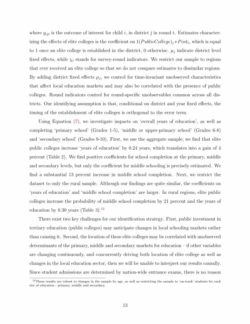
Using Equation (7), we investigate impacts on ‘overall years of education’, as well as

completing ‘primary school’ (Grades 1-5), ‘middle or upper-primary school’ (Grades 6-8)

and ‘secondary school’ (Grades 9-10). First, we use the aggregate sample; we find that elite

public colleges increase ‘years of education’ by 0.24 years, which translates into a gain of 4

percent (Table 2). We find positive coefficients for school completion at the primary, middle

and secondary levels, but only the coefficient for middle schooling is precisely estimated. We

find a substantial 13 percent increase in middle school completion. Next, we restrict the

dataset to only the rural sample. Although our findings are quite similar, the coefficients on

‘years of education’ and ‘middle school completion’ are larger. In rural regions, elite public

colleges increase the probability of middle school completion by 21 percent and the years of

education by 0.30 years (Table 3).12

There exist two key challenges for our identification strategy. First, public investment in

tertiary education (public colleges) may anticipate changes in local schooling markets rather

than causing it. Second, the location of these elite colleges may be correlated with unobserved

determinants of the primary, middle and secondary markets for education – if other variables

are changing continuously, and concurrently driving both location of elite college as well as

changes in the local education sector, then we will be unable to interpret our results causally.

Since student admissions are determined by nation-wide entrance exams, there is no reason

12These results are robust to changes in the sample by age, as well as restricting the sample to ‘on-track’ students for eachtier of education - primary, middle and secondary.

13

to believe that the establishment of these colleges is driven by anticipated future changes

in specific local schooling markets. With the inclusions of district fixed effects, the more

relevant concern is whether location may be correlated with preexisting trends in education

markets, if these colleges are introduced to areas which are changing more rapidly. For

instance, rapid industrialization may drive both the location of these elite colleges as well

as changes to education decisions. However, these variables are likely to change gradually

over time rather than suddenly or all at once, therefore we might expect these effects to be

evident in the form of preexisting trends in data.

First, as a robustness check we test the stability of our coefficients of interest by in-

cluding a variety of controls. We start with our baseline specification, gradually adding age

fixed effects, log of household consumption, and district-specific linear trends. Although the

explanatory power of our specifications increases, these controls do not substantively affect

our coefficients of interest, plausibly indicating that the year of entry of elite public colleges

might not be correlated with other unobserved variables (Altonji et al., 2005; Oster, 2016).

Results are presented in Tables 4 and 5.

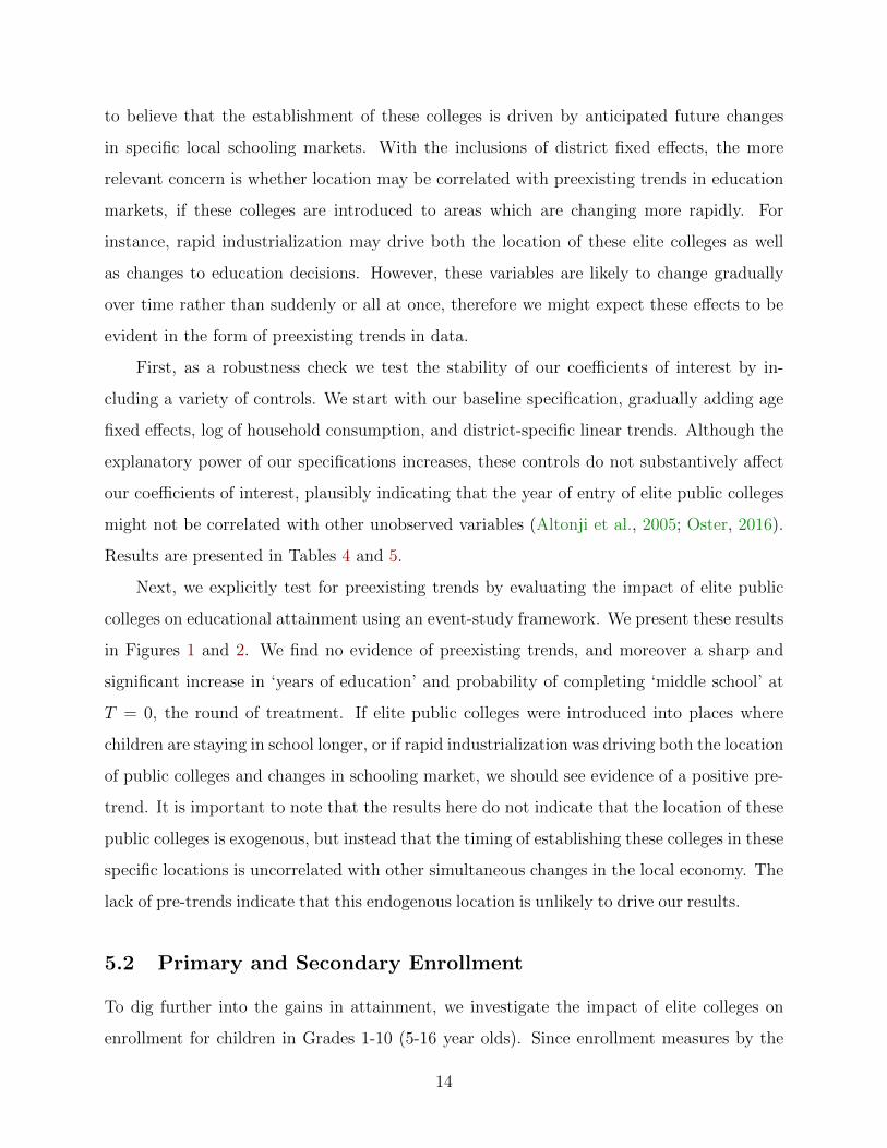
Next, we explicitly test for preexisting trends by evaluating the impact of elite public

colleges on educational attainment using an event-study framework. We present these results

in Figures 1 and 2. We find no evidence of preexisting trends, and moreover a sharp and

significant increase in ‘years of education’ and probability of completing ‘middle school’ at

T = 0, the round of treatment. If elite public colleges were introduced into places where

children are staying in school longer, or if rapid industrialization was driving both the location

of public colleges and changes in schooling market, we should see evidence of a positive pre-

trend. It is important to note that the results here do not indicate that the location of these

public colleges is exogenous, but instead that the timing of establishing these colleges in these

specific locations is uncorrelated with other simultaneous changes in the local economy. The

lack of pre-trends indicate that this endogenous location is unlikely to drive our results.

5.2 Primary and Secondary Enrollment

To dig further into the gains in attainment, we investigate the impact of elite colleges on

enrollment for children in Grades 1-10 (5-16 year olds). Since enrollment measures by the

14

type of school come from annual data (ASER), we utilize a flexible event-study framework

and estimate the following linear probability model:

yijt =−2∑

τ=−8

βτ1(t− T ∗j = τ) +0∑

τ=9

βτ1(t− T ∗j = τ) + αi + µj + χt + εijt (8)

where yijt is 1 if the child i is the outcome of interest in district j in year t = 2006,...,2014,

0 otherwise. Estimates characterizing the effects of elite colleges are the coefficients on the

event-year dummies, 1(t − T ∗j = τ), which are equal to 1 when the year of observation is

τ = −8, ..., 0, ..., 9 years from T ∗j , the date when the elite college was established in district

j (τ = −1 is omitted). αi indicate child age dummies, µj indicate district level fixed effects,

while χt stands for year indicators. Here too, we restrict our sample to regions that ever

received an elite college so that we do not compare estimates to dissimilar regions.

Before we present our results, it is important to note that the proportion of children

‘currently enrolled’ at the baseline (T = −1) was close to 95%, therefore gains in educational

attainment are likely driven by a reduction in later-year drop-outs.13 In Figure 5 we present

impacts on overall enrollment. While there is no immediate or short-run increase in overall

enrollment, enrollment is slightly higher by T = 2. This small increase in overall enrollment,

however, hides significant changes in where these students are going to school.

In Figure 3 we report the impact of elite public colleges on public school enrollment. The

coefficient in the year of treatment, the year when elite public colleges were established is -

0.05, which means that, public colleges led to a 5 percentage point decrease in the probability

of public school enrollment. These effects get larger in the medium term. In Figure 4 we

report the coefficients for private school enrollment. Elite public colleges are associated with

an increase of 5 percentage points in the probability of private school enrollment in the year

of treatment, and over 10 percentage points by year 4.14 Overall, these results suggest that

children are switching from public to private schools in response to the entry of elite public

colleges, and staying in school longer.

13Furthermore, we estimate impacts on current-grade and grade dropped-out. If children were staying in school longer, wewould find an increase in both. Indeed, we find support for such an hypothesis, results are presented in Figures A.2 and A.3.Impacts on both these variables are gradual, and in the medium term, ‘current-grade’ increases by 0.16, and ‘grade dropped-out’by 0.48.

14In Figures A.24-A.29 we look at heterogenous impacts on public, private and overall enrollment by age and gender, we findsimilar estimates for younger and older, and male and female students.

15

We find no evidence of a preexisting trend in any of our estimates. Indeed, the trend

break in the left-hand side variable at T = 0 is apparent and economically and statistically

significant for both public and private enrollment. The estimates of the pre-treatment periods

are small in magnitude and statistically indistinguishable from zero. As a robustness check,

in Figures A.4, A.5 and A.6 we add district-specific linear trends and estimate Equation (8).

Our results remain unaffected.15

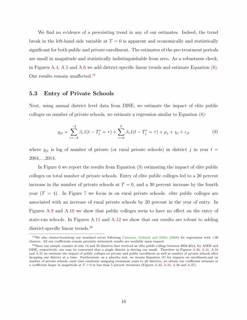
5.3 Entry of Private Schools

Next, using annual district level data from DISE, we estimate the impact of elite public

colleges on number of private schools, we estimate a regression similar to Equation (8):

yjt =−2∑

τ=−8

βτ1(t− T ∗j = τ) +0∑

τ=9

βτ1(t− T ∗j = τ) + µj + χt + εjt (9)

where yjt is log of number of private (or rural private schools) in district j in year t =

2004,...,2014.

In Figure 6 we report the results from Equation (9) estimating the impact of elite public

colleges on total number of private schools. Entry of elite public colleges led to a 20 percent

increase in the number of private schools at T = 0, and a 30 percent increase by the fourth

year (T = 4). In Figure 7 we focus in on rural private schools: elite public colleges are

associated with an increase of rural private schools by 20 percent in the year of entry. In

Figures A.9 and A.10 we show that public colleges seem to have no effect on the entry of

state-run schools. In Figures A.11 and A.12 we show that our results are robust to adding

district-specific linear trends.16

15We also cluster-bootstrap our standard errors following Cameron, Gelbach and Miller (2008) for regressions with <30clusters. All our coefficients remain precisely estimated; results are available upon request.

16Since our sample consists of only 14 and 23 districts that received an elite public college between 2004-2014, for ASER andDISE, respectively, one may be concerned that a single district is driving our result. Therefore in Figures A.30, A.31, A.34and A.35 we estimate the impact of public colleges on private and public enrollment as well as number of private schools afterdropping one district at a time. Furthermore, as a placebo test, we iterate Equation (8) for impacts on enrollment,and onnumber of private schools, each time randomly assigning treatment years to all districts, we obtain our coefficient estimate ora coefficient larger in magnitude at T = 0 in less than 5 percent iterations (Figures A.32, A.33, A.36 and A.37).

16

6 Mechanisms

In this section, we find compelling evidence that infrastructure upgrades are an important

impact pathway. Public colleges increase the supply of private schools by lowering the setup

costs through infrastructure upgrades in the region. When private schools enter areas with

few public schools, households sensitive to travel costs will transfer their children to these

private schools, enabling the marginal student to stay in school longer.

6.1 Infrastructure Upgrades

Comparative statistics from our model suggest that a decrease in entry or set-up costs

for private schools shift the supply curve outwards (dQSy/dz1|p < 0; dQSy/dz2|p < 0).

If elite public colleges cause an increase in access to local public infrastructure, then this

would cause an entry of new private schools. To find evidence for this prediction, we first

estimate the effects of elite public college on village-level night-time lights, as a proxy for

rural electrification. Here, we take advantage of the granularity of our village level night-

lights data; using latitude-longitude coordinates of elite public colleges and over 500,000

villages across India, we calculate the distance of every village to the nearest elite college

from 2001-2011, and estimate the following equation:

yijt =15∑

τ=−1

βτ1(m <= DistancetoCollege < n)ijt + µi + χt + εijt (10)

where m = 0, 10, ..., 140 and n = m + 10 kms. yijt is log mean night lights in village i,

district j, year t. Estimates characterizing the effects of elite colleges are the coefficients

on the distance to college dummies, 1(m <= DistancetoCollege < n)ijt, which are equal

to 1 if distance of village i in district j in year t to the closest elite college is between 0-10

kms, 10-20 kms and so on, till 140-150 kms; 1(150 <= DistancetoCollege)ijt is the omitted

category. µi indicate village level fixed effects, while χt stands for year dummies.17 Our

identifying assumption is that, conditional on village and year fixed effects, the change in

the distance of villages to the closest elite college is orthogonal to the error term.

17Our distance variable is constructed using village and elite public college location geocodes. For elite public colleges, weuse geocodes corresponding to their (eventual) permanent location, even in cases where the campus is under construction.

17

In Figure 8 we present results from Equation (10). The coefficient for

1(0 <= DistancetoCollege < 10)ijt is 0.15, which means that, villages, which after entry of

an elite college, are now within 10 kms from the new college, see a 15 percent increase in

mean night light brightness. The effect decreases with an increase in distance to the nearest

elite public college. This result suggests that elite public colleges led to increases in the

access to electricity.

Next, we provide additional evidence on the impacts on public infrastructure by directly

estimating the effects of elite public college on access to electricity and tap water using Census

Village Directories in 2001 and 2011 within a simple difference-in-differences framework. We

estimate the following equation:

yijt = β11(PublicCollege)j × Postt + µj + Postt + εijt (11)

where yijt is 1 if a village has access to electricity for agricultural use (or access to tap water),

0 otherwise. µj indicate district fixed effects, while Postt = 1 is the 2011 dummy, and

1(PublicCollege)j = 1 if the region received a public college between 2001 and 2011.

We present these results in Figure 9. Elite public colleges lead to a 18 percentage

point increase in the probability of electricity access and 7 percentage point increase in the

probability of access to tap water. We test the implicit parallel trends assumption by looking

at pre-trends in Figure A.13 and A.14, and more formally in Table A.17.

Lastly, we match village-level infrastructure indicators from Census Village Directories

in 2001 and 2011 with village-level geocodes and estimate Equation (10):

yijt =10∑

τ=−1

βτ1(m <= DistancetoCollege < n)ijt + µj + χt + εijt (12)

where m = 0, 10, ..., 100 and n = m + 10 kms. Here 1(100 <= DistancetoCollege)ijt is

the omitted category and µj indicate district fixed effects, while χt stands for year dummies

as before. We present these results in Figures A.15 and A.16. The agriculture electricity

results are largely consistent with the night lights results, and villages closer to an elite

college are more likely to have access to tap water. Overall, our results seem to suggest that

18

in poorer countries like India, public colleges lead to investments in public infrastructure,

and that these infrastructure upgrades reduce set-up costs for private schools, facilitating

their entry.

6.1.1 Travel Costs: Heterogeneity by Number of Public Schools

Even if infrastructure upgrades induce entry of private schools, there will be no transfers from

public to private schools if the demand for private schooling is inelastic and insensitive to the

costs of attending school. Predictions from our model suggest that decreases in travel costs

to attend private schools increase the demand for private schooling (dQd/dTp < 0), and that

the demand for private schooling increases with distance to public schools (dQd/dTs > 0).

In the empirical analysis so far, we find that elite public colleges lead to a decrease in public

school enrollment and an increase in private school enrollment, with mild effects on overall

enrollment in the medium term. If elite public colleges are set-up in districts where attending

public schools is costly due to travel costs, then an increase in the number of private schools

in such regions will cause children to switch from public to private schools, and stay in

school longer. Such a hypothesis relies on the relationship between elite public colleges,

private schools, household school choice and educational attainment in regions with fewer

public schools.

Private Schools: Kremer and Muralidharan (2008) and Pal (2010) find that private

schools are more likely to be present in villages with poorly functioning government schools.

Similarly, our model suggests that districts with fewer government schools will have a greater

number of private schools (dp/dTs > 0 and dN1/dTs > 0). Furthermore, elite college entry in

response to lower set-up costs is greater when there are fewer government schools (ddQsydz1|p

dTs<

0). To empirically test this relationship, we divide treatment districts in two samples at the

median number of state-run schools in T = −1: districts with a large number of public schools

(above the median), and those with a fewer number of public schools (below the median).

We estimate Equation (9) on both these samples. We find evidence for a substantially larger

increase in the number of private school in districts with fewer government schools (Figure

A.22).

19

Enrollment: Next, we investigate impacts on private school enrollment in districts

with fewer state-run schools. Districts with fewer public schools, ‘pre-treatment’, should see

a larger increase in the number of switchers. We estimate Equation (8) for two samples,

split by number of government schools ‘pre-treatment’ in T = −1, and find that elite public

colleges lead to a substantially larger increase in private school enrollment (Figure 11), and

concurrently a large decrease in public school enrollment, in districts with fewer public schools

(Figure 10) for the first three years immediately following the entry of elite colleges.

Educational Attainment: In Section 5.1, we find that the increase in educational

attainment is concentrated at the middle school level. However, if new private schools enter

the education market, solving a cost constraint by lowering transportation costs, that should

enable children to stay in school longer at all levels of schooling, unless the new private

schools only offer middle schooling. To unpack these results, we look at the type of private

schools that entered the market following elite public colleges. In Figures A.20 and A.21, we

separately evaluate the impact on number of private schools that only offer primary schooling,

and on number of private schools that also (or only) offer upper-primary education and above.

We find that, in rural areas, the increase in private schools, documented in Section 5.3, is

driven by schools offering upper-primary or a combination of primary and upper-primary

schooling. We don’t find an increase in number of private schools that only offer primary

education.18 Thus, it is possible that only students who have completed primary schooling

at a state-run school are switching (or rather moving on) to new private schools that offer

middle-school education. Those students were previously cost constrained, moved to private

middle schools that are closer, increasing attainment only at the middle school level.

If only children in a certain age segment were moving to private schools, such an ex-

planation would be plausible. But, we do not find any heterogeneity in switchers by age

group. Therefore, we should expect to see an increase in attainment at all levels of edu-

cation. First, it is important to note that, although imprecise, coefficients for primary and

18In the aggregate sample, we do find an increase in private schools only offering primary education, however, the magnitudeof increase in number of schools offering upper-primary schooling or above is almost twice as high. It is theoretically possiblethat private schools that were previously only offering primary education are now also offering upper-primary education, andthis is being picked up by our results. We don’t think that is the case here, since, we don’t find a decrease in either theaggregate number of private schools, those located in rural areas, or schools that only offer primary education. Thus, for sucha situation to exist, a large proportion of new private schools must only offer primary schooling and an even larger proportionof the existing private schools must have started offering upper-primary education.

20

secondary completion are positive, 2% and 13% increase in primary and secondary school

completion respectively. Second, in order to further investigate impacts on educational at-

tainment, we rely on guidance from our enrollment results. Specifically, we find that districts

with fewer government schools in T = −1, see a significantly larger increase in probability of

switching from public to private schools. Thus, if our hypothesis is correct, we should expect

a larger increase in educational attainment, at all levels of schooling, in districts with fewer

government schools before treatment. So, we divide the NSS sample by number of state-run

schools offering upper-primary education or above in T = −1, and evaluate the impacts of

elite public colleges on educational attainment.19 Tables 10 and 11 present our results. In

districts with fewer state-run schools, we find large and precise estimates; elite public colleges

increase years of education by 0.84 years (15%), probability of primary school completion by

13 percentage points (19%), middle school completion by 12 percentage points (33%), and

secondary school completion by 9 percentage points (70%).20

6.2 Alternative Explanations

In this section, we discuss some alternative channels that could potentially explain the ob-

served relationship between public colleges and schooling outcomes. Specifically, we consider

four alternative explanations: (1) increase in population, (2) income effect, (3) demand exter-

nalities, and (4) powerful politician hypothesis. While we find little support for these expla-

nations, we cannot conclusively rule out demand externalities and aspirational effects.

6.2.1 Increase in Population: dp/dM > 0 ; dN1/dM > 0

Demand for all schooling (both public and private) increases with population, raising equilib-

rium fee (tuition) and the number of private schools. Thus, if public colleges cause migration

into the district, it may increase the number of private schools.

Elite public colleges can create jobs, and incentivize immigration into these districts.

19We divide the sample by number of schools offering upper-primary education because one, we are interested in impacts onall levels of schooling and not just primary schooling and two, because almost all the increase in private schools was driven byschools that offered upper-primary education or above. Lastly, we also find that the increase in new private schools offering atleast upper-primary schooling is larger in districts with fewer government schools offering upper-primary education or above(Figure A.23).

20These results are largely consistent even when we split the sample by number of public schools proportional to districtpopulation between age 5 and 16 years.

21

This could mean other jobs in the college itself, jobs working for college employees or newly

created jobs in existing firms/industries that enjoy synergies with these academic institutions.

If people migrate into these areas for these jobs, it could increase the demand for schooling

(dN1/dM > 0). Furthermore, if their children are more ‘able’ then, that will also increase

demand for schooling (dN1/dδ > 0). Both will lead to an entry of private schools.

We directly look at impacts on population in districts where a new elite public college

was set-up. We use data from village census directories and district population censuses, 2001

and 2011, to estimate the following equation in a difference-in-differences framework:

yijt = β11(PublicCollege)j × Postt + µj + Postt + εijt , (13)

where yijt is log of population in village i (or district j), in year t; µj indicate district fixed

effects, while Postt = 1 if the year is 2011, and 1(PublicCollege)j = 1 if the region received

a public college between 2001 and 2011.

We present these results in Figure 9. Consistent with the literature on low spatial

mobility in rural India (Munshi and Rosenzweig, 2009), we find almost no change in village

population in districts that received an elite public college. Moreover, total population

remains unchanged (Table A.29). Lastly, we look at the effect of public colleges on different

age groups in the Tables A.30 - A.34; we fail to find evidence for an increase in population

for any age group in districts that received an elite public college.21

Children of Faculty and Staff at Elite Public Colleges: dp/dδ > 0 ; dN1/dδ > 0

An increase in the ability of the students will increase the demand for all schooling, raise

market price (tuition) and induce more private schools to enter the market. If children of

faculty from these public colleges are more ‘able’, then public colleges will lead to an increase

in the number of private schools in the district.

We explore if children of faculty and staff alone can explain our results. If an elite public

college employs a large number of faculty and staff, or if their children are more ‘able’, then

21Using NSS data, we also estimate the effect of elite public colleges on educational attainment for individuals between 20-35.If there were an influx of educated workers for jobs into these districts, we would capture such an effect through an increasein probability of completing primary, middle, secondary or undergraduate education. We fail to find any such evidence (TableA.26, A.27, A.28).

22

public colleges will lead to an increase in the number of private schools in the district . We

don’t think the addition of these children alone can explain the magnitude of increase in

number of private schools. We find an increase of almost 20 percentage points in the number

of private schools in year of treatment; in 2004, the mean number of private schools in

districts that received a public college between 2004-2014, was 350. So, a 20 percent increase

means at least 70 new schools. From DISE, we know that each private school enrolls 200

students each, on average. So a substantial number of new faculty will have to migrate

with the new public college to explain this result. Information obtained from these colleges

indicate that on average these colleges have around 150 faculty members, so increases in the

‘ability’ of the local student population due to influx of faculty would only explain 1% of the

increase in number of private schools.22

Supply of School Teachers: If students graduating from elite public colleges were

opening-up new private schools in the district, and working as school teachers in these

schools, it could also potentially explain our results. For instance, Andrabi, Das and Khwaja

(2013) show that private schools in Pakistan are three times more likely to emerge in villages

with government girls’ schools due to an increase in supply of teachers. We do not find

evidence for such an explanation. First, since the first batch of students in these colleges

would only graduate after 2-4 years, if an increase in the supply of teachers due to students

graduating from elite public colleges was driving our results, we would not see an immediate

increase in number of private schools, and probability of enrollment in these schools. Second,

it is important to note that a large proportion of students graduating from elite public

colleges are employed by technology or management firms in major Indian cities (Willis-

Tower-Watson, 2016). So, such supply-side channels are less relevant for our context.

22There are three additional points of note. Firstly, here we look at total private schools and not just rural private schoolssince faculty are more likely to live in more urban areas. However, even if we assume that all faculty at new elite publiccolleges live in rural areas, the increase in the number of rural private schools cannot be explained by increases in the ‘ability’of children in the district due to influx of children of faculty at these public colleges. Secondly, in order to confirm that facultymembers do not form a large proportion of the treatment district, using NSS data, we estimate the impact of public collegeson the probability of being a college teacher. We find no effect (Table A.23). Lastly, we also do not think that children ofstudents at these public colleges can explain our results. At any point of time, elite public colleges in our sample have around600-800 students on average, and in most colleges almost 70 percent of them are undergraduates. Elite public colleges thatare primarily post-graduate institutions have around 300 students on average. Also, if these students formed a large enoughportion of the local population, we should see an increase in probability of completing an undergraduate degree. We formallytest this hypothesis, and find no effect (Table A.21).

23

6.2.2 Income Effect: dp/dln(w) > 0 ; dN1/dln(w) > 0

An increase in income increases the demand for all schooling (both public and private), rais-

ing the equilibrium fees charged as well as the number of private schools. If the establishment

of public colleges increases incomes, it may lead to private school entry.

Previous studies have suggested that regional characteristics have a critical impact on

the locational decisions made by new firms. Moreover, (Audretsch, Lehmann and Warning,

2005) identifies the presence of a university as such a locational factor. There exist several

linkages between academic institutions and the local economy (Adams, 2001; Basant and

Chandra, 2007), and academic institutions can play a significant role in the local economic

development. Elite public colleges can increase incomes of existing local population by

creating high-paying jobs, thus driving entry of private schools.

Furthermore, if elite public colleges increase access to electrification and tap water, these

infrastructure upgrades could also increase expenditure or earnings. In addition to being

useful as proxies for electrification, nighttime lights have been used by economists as an

indicator for economic development, especially in developing countries that have issues with

disaggregated income data (Chen and Nordhaus, 2014; Henderson and Storeygard, 2009).

So, it is possible that impacts on nighttime lights are in fact income effects.

To find evidence for these hypothesis, we use NSS data to estimate Equation (7) to study

the effects of public colleges on consumption expenditure and earnings. Table A.22 presents

the impacts of public colleges on household expenditure and wages. We find no effects on

consumption expenditure or wages for the aggregate or rural sample. Next, we investigate

effects on earnings and employment by occupation – agriculture and mining, manufacturing,

construction and services (Tables A.24 and A.25). We fail to find evidence for an increase

in employment or earnings for any occupation.

It is possible that a more granular identification strategy like the one used for village-

level night-time lights will be able to tease out these income effects. In order to test this,

we estimate Equation (12) for village-level population using Census Village Directories in

2001 and 2011. We do not find evidence for an increase in population in villages closest

to the elite public college (Figure A.17). Lastly, using per capita expenditure and earning

24

data from Census Village Directory in 2001, we evaluate if villages closest to an elite public

college had higher per capita expenditure or earnings. We do not find support for such a

result (Figure A.18).

6.2.3 Demand Externalities: dp/dθ > 0 ; dN1/dθ > 0 or Returns to Education:

dp/dr > 0 ; dN1/dr > 0

Increases in the actual or perceived returns to education or other demand externalities (either

via peer effects, information or role model effects) will raise demand for all schooling, raise the

market price (tuition) and induce more private schools to enter the market. Public colleges

may increase the actual or perceived returns to education by creating new employment

opportunities or raise aspirations of the rural poor. Either scenario will increase overall

demand for schooling and encourage entry of private schools.

Elite public colleges are considered extremely prestigious, and close proximity might

make them even more salient, or increase salience of higher education in general, thus raising

educational aspirations of children in the region. Moreover, entry of public colleges might

also alter local perceptions about returns to education due to information spillovers, causing

an increase in the demand for schooling. If public schools are unable to meet this increased

demand, private schools may enter the region. While we cannot conclusively rule out these

mechanisms, we find little evidence in support.

First, for such an explanation to be driving our results, we would expect an increase in

both public and private school enrollment. However, we observe a decrease in public school

enrollment. Next, we test these hypotheses by looking at test scores from the ASER data.

Since, we do not know of district level dataset that captures aspirations in India, we use

test scores as a weak proxy for aspirations. If household aspirations or their perception of

returns to education increase due to public colleges, then we could expect that to translate

into higher test scores. ASER surveyors ask each child four potential questions in math

and reading (in their native language). In each subject, they begin with the hardest of four

questions. If a child is unable to answer that question, they move on to the next easiest

question and so on and so forth. We estimate Equation (8) to investigate the impacts of

public colleges in both math and reading scores. We do not find an effect on either math or

25

reading scores (Figures A.7 and A.8).

Access to Higher Education: Test scores won’t capture an increase in demand for

schooling that is driven by access to higher education. Empirical evidence from the United

States suggests that college proximity increases local college enrollment (Card, 1993; Currie

and Moretti, 2003; Lapid, 2016). Thus, it is possible that proximity to an institute of higher

education increases the demand for primary and secondary schooling as well, driving our

results. First, in Section 5.2, we only find a small increase in enrollment in the medium term.

Next, we highlight the institutional features of elite public colleges. Unlike ‘regular’ colleges,

admission into elite public colleges in India is determined by an extremely competitive nation-

wide entrance exams. For instance, elite colleges such as the Indian Institutes of Technology

(IITs) have an acceptance rate of 2 percent from a pool of roughly 500,000 students who

qualify to take the entrance exam. Thus, we do not think that this is a likely explanation

for our results.

6.2.4 Powerful Politician Hypothesis:

In a developing country like India, it is necessary that we address the influence of political

clout as an explanation for our results. It is possible that powerful local politicians success-

fully lobby the federal government for both elite public colleges, and infrastructure upgrades

in their constituency or district. This would mean that our results are driven by powerful

politicians, and not by elite public colleges. Although, such an explanation is compatible

with supply-side factors, we do not find strong evidence for such an hypothesis. First, unless

these ‘powerful politicians’ align timing of infrastructure upgrades with entry of elite pub-

lic colleges, we would find evidence for it in the form of preexisting trends in our outcome

variables. Second, out of the 42 districts that received an elite college between the period

2004-2014, almost 50% were represented by members from the opposition and not the ruling

coalition, the Indian National Congress or its allies. Moreover, out of the 22 districts rep-

resented by members from the ruling coalition, more than 40% were first time Members of

Parliament. It is reasonable to assume that experienced MPs from the ruling coalition enjoy

the most ‘influence’; however, since only 14 out of the 42 districts had MPs from the ruling

26

coalition serving a second term or higher, political clout doesn’t seems to play a significant

role in the location of these elite colleges. Third, and most importantly, our results are

robust to dropping districts governed by such ‘powerful’ MPs from the sample.23

6.3 Discussion

After thoroughly examining several mechanisms through which elite public colleges may

affect the market for primary and secondary education, we find support for supply-side

channels across multiple datasets. First, we find that elite public colleges cause an increase

in access to public infrastructure. It is likely that these infrastructure upgrades reduce

set-up costs for for-profit private schools. Next, we find that the magnitude of transfers

from public to private schools and the increase in educational attainment are substantially

larger in regions with fewer public schools. These results suggest that new private schools

are solving a cost constraint by lowering cost of attendance, and specifically, travel costs,

enabling children to stay in school longer. Although a chain of events emerges from these

set of results, our conclusions are only suggestive. Although, we fail to find strong evidence

for alternative mechanisms, we can’t completely rule them out.

However, given the evidence at hand, we propose the following sketch of school choice

as the simplest explanation for our results. First an elite public college is introduced to a

region. Assume that the region has only one public school and two identical enrollees, one

that lives closer to the public school and the other that lives next to the elite public college.

A for-profit private school that witnesses public investment in infrastructure, enters the

region, locating close to the elite public college, and therefore near one of the students. This

student transfers to private schools, while the other remains in the public school. Moreover,

because the private school solves a cost constraint for the ‘transfer student’ by being closer,

instead of dropping out of school at the following year, she decides to stay enrolled for more

years.

Implicit in such an explanation is the key assumption that private schools enter areas

with good public infrastructure. We have already shown evidence that elite public colleges

increase access to public infrastructure and number of private schools, with a larger increase

23Results are available on request.

27

in number of private schools in areas with fewer public schools. Now, we test this assumption

at the village-level using the 2011 Census Village Directory. It contains indicators for the

presence of public and private schools for each village in India. We estimate Equation (12)

and find additional evidence in support of this assumption. In Section 6.1, we showed that

elite colleges cause the largest increase in access to public infrastructure in villages closest

to elite colleges. Accordingly, we find that villages closest to elite public college are more

likely to have a private school. (Figure 12).

7 Conclusion

In this paper, we argue that public investment in higher education also facilitates the educa-

tion of school children in India. We show that public colleges have positive spillover effects on

primary and secondary education markets in India. Elite public colleges encourage the entry

of private schools, and increase enrollment in cost-effective private schools at the expense

of state-run schools. Overall, our results translate into gains in educational attainment as

children stay enrolled in school longer. We also conduct a back-of-the-envelope calculation

to compare the direct benefits of these institutions, through training of undergraduate and

graduate students, to indirect benefits accrued due to gains in efficiency and educational

attainment. We find that such indirect benefits of elite public colleges are at least 48% of

direct benefits.

Moreover, institutional features of these elite public colleges, guidelines that characterize

their ‘placement’, and a set of consistent results across multiple datasets, help us contribute

to the literature on the determinants of private provision of education, household school

choice and educational attainment in developing countries. First, we show that elite public

colleges cause an increase in the number of private schools, and evidence that suggests that

investment in public infrastructure is the likely mechanism of impact. This suggests that

public investment in infrastructure reduces set-up costs for for-profit private schools, encour-

aging private participation in educating low-income households. Second, we find that elite

public colleges lead to gains in educational attainment, and transfers from public to private

schools, and both these effects are larger amongst districts with fewer state-run schools.

28

These findings highlight the importance of the costs of attending school, and specifically

transportation costs, in household school choice and educational attainment.

As we think about policy implications, we would like to highlight that elite public

colleges led to highly localized, and large investments in public infrastructure. For instance,

villages closest to elite public colleges also saw an increase of over 15% in access to tap water.

Furthermore, our estimates from nighttime lights suggest that villages closest to elite public

colleges experienced an increase of 1 to 3 units in nighttime brightness. These magnitudes

are quite large. In comparison, a village electrification program in India increased nighttime

light brightness by 0.15 units at the village level (Burlig and Preonas, 2016). However, they

find no effects of electrification on educational attainment. While, our difference-in-difference

estimates suggests that elite public colleges increased years of schooling by 0.3 years at the

district level. These results suggest that construction of public colleges in poorer regions, by

facilitating a suite of focal infrastructure investments, may have larger development impacts

compared to last mile programs that target specific services.

29

References

Adams, James. 2001. “Comparative Localization of Academic and Industrial Spillovers.”NBER Working Paper.

Adukia, Anjali, Sam Asher, and Paul Novosad. 2016. “Educational Investment Re-sponses to Economic Opportunity: Evidence from Indian Road Construction.” WorkingPaper.

Aghion, P, L Boustan, C Hoxby, and J Vandenbussche. 2009. “Causal Impact ofEducation on Economic Growth : Evidence from U.S.” Working Paper, , (March).

Aiyappa, Manu. 2015. “Political tug of war on cards for location of IIT in Karnataka.”The Times of India.

Alderman, Harold, Peter F Orazem, and Elizabeth M Paterno. 2001. “SchoolQuality , School Cost , and the Public / Private School Choices of Low-Income Householdsin Pakistan.” Journal of Human Resources, 36(2): 304–326.

Altonji, Joseph G, Todd E Elder, Christopher R Taber, Source Journal, NoFebruary, Joseph G Altonji, Todd E Elder, and Christopher R Taber. 2005.“Selection on Observed and Unobserved Variables : Assessing the Effectiveness of CatholicSchools.” Journal of Political Economy, 113(1): 151–184.

Andrabi, Tahir, Jishnu Das, and Asim Ijaz Khwaja. 2013. “Students today, teach-ers tomorrow: Identifying constraints on the provision of education.” Journal of PublicEconomics, 100: 1–14.

Audretsch, David B., Erik E. Lehmann, and Susanne Warning. 2005. “Universityspillovers and new firm location.” Research Policy, 34(7): 1113–1122.

Barro, Robert J. 2001. “Human Capital and Growth.” The American Economic Review,Papers and Proceedings of the Hundred Thirteenth Annual Meeting of the American Eco-nomic Association, 91(2): 12–17.

Basant, Rakesh, and Pankaj Chandra. 2007. “Role of Educational and R&D Institutionsin City Clusters: An Exploratory Study of Bangalore and Pune Regions in India.” WorldDevelopment, 35(6): 1037–1055.

Birdsall, Nancy. 1982. “Child Schooling and the Measurement of Living Standards.” LivingStandards Mesurement Study.

Birdsall, Nancy. 1985. “Public Inputs and Child Schooling in Brazil.” Journal of Devel-opment Economics, 18: 67–86.

Bobonis, Gustavo J, and Frederico Finan. 2009. “Neighborhood Peer Effects in Sec-ondary School Enrollment Decisions.” Review of Economics and Statistics, 91(4): 695–716.

30

Burde, Dana, and Leigh L. Linden. 2013. “Bringing education to afghan girls: A ran-domized controlled trial of village-based schools.” American Economic Journal: AppliedEconomics, 5(3): 27–40.

Burlig, Fiona, and Louis Preonas. 2016. “Out of the Darkness and Into the Light?Development Effects of Rural Electrification.” Working Paper, , (October).

Cameron, Colin, Jonah B. Gelbach, and Douglas L. Miller. 2008. “Bootstrap-BasedImprovements for Inference with Clustered Errors.” Review of Economics and Statistics,90(3): 414–427.

Cantoni, Davide, and Noam Yuchtman. 2014. “Medieval Universities, Legal Insitutions,and Commercial Revolution.” Quarterly Journal of Economics, , (2009): 823–887.

Card, David. 1993. “Using Geographic Variation in College Proximity to Estimate theReturn to Schooling.” NBER Working Paper.

Carneiro, Pedro, Hugo Reis, Pedro Carneiro, and Hugo Reis. 2016. “The Value ofPrivate Schools : Evidence from Pakistan.” Working Paper.

Carneiro, Pedro, Jishnu Das, and Hugo Reis. 2015. “Parental Valuation of SchoolAttributes in Developing Countries: Evidence from Pakistan.” Working Paper.

Chand, T. R. Kiran, K. V. S. Badarinath, C. D. Elvidge, and B. T. Tuttle.2009. “Spatial characterization of electrical power consumption patterns over India usingtemporal DMSP-OLS night-time satellite data.” International Journal of Remote Sensing,30(3): 647–661.

Chen, Xi, and William D Nordhaus. 2014. “Using luminosity data as a proxy foreconomic statistics.” Proceedings of the National Academy of Sciences, 108(45): 8589–8594.

Currie, Janet, and Enrico Moretti. 2003. “Mother’s Education and the IntergenerationalTransmission of Human Capital: Evidence from College Openings.” The Quarterly Journalof Economics, 118(4): 1495–1532.

Das Gupta, Monica, Robert Engelman, Jessica Levy, Gretchen Luchsinger, TomMerrick, and James E. Rosen. 2014. “The Power of 1.8 billion Adolescents, Youthand the Transformation of the Future.” UNFPA State of World Population.

Davidson, Max. 2010. “1,000 new universities for India?” Telegraph.co.uk.

Donaldson, Dave. 2017. “Railroads of the Raj: Estimating the Impact of Transport In-frastructure.” The American Economic Review, Forthcoming.

Duflo, Esther. 2001. “Schooling and Labor Market Consequences of School Construction inIndonesia : Evidence from an Unusual Policy Experiment.” American Economic Review,91(4): 795–813.

31

Duflo, Esther, and Rohini Pande. 2007. “Dams.” The Quarterly Journal of Economics,, (May): 601–646.

Henderson, J Vernon, and Adam Storeygard. 2009. “Measuring Economic Growthfrom Outer Space.” Economic Analysis, 102(2): 1–53.

Hiremath, Gourishankar S, and H.S. Komalesha. 2017. “How IITs Turned FromNehru ’ s Vision of Technology To Catering Engineers for MNCs.” The Wire, 1–18.

Kantor, Shawn, and Alexander Whalley. 2014. “Knowledge Spillovers from ResearchUniversities: Evidence From Endowment Value Shocks.” Review of Economics and Statis-tics, 96(1): 171–188.

Khanna, Gaurav. 2015. “Large-scale Education Reform in General Equilibrium: Regres-sion Discontinuity Evidence from India.” Job Market Paper.

Kingdom, Geeta Gandhi. 1998. “Does The Labour Market Explain Lower Female School-ing in India.” The Journal of Development Studies, 35(1): 39–65.

Kline, Patrick, and Enrico Moretti. 2014. “Local Economic Development, Agglomer-ation Economies, and the Big Push: 100 Years of Evidence from the Tennesse ValleyAuthority.” The Quarterly Journal of Economics, 129(1): 275–331.

Kremer, Michael, and Karthik Muralidharan. 2008. “Public and Private Schools inRural India.” School choice international: Exploring public-private partnerships, 91–110.

Lapid, Patrick A. 2016. “Expanding College Access : The Impact of New Universities onLocal Enrollment.” Job Market Paper.

Lavy, Victor. 1996. “School supply constraints and children’s educational outcomes in ruralGhana.” Journal of Development Economics, 51(2): 291–314.

Lillard, Lee A, and Robert J Willis. 1994. “Intergenerational Educational MobilityEffects of Family and State in Malaysia.” The Journal of Human Resources, 29(4): 1126–1166.

Lipscomb, Molly, Mushfiq Mobarak, and Tania Barham. 2011. “Development Effectsof Electrification : Evidence from the Geologic Placement of Hydropower Plants in Brazil.”American Economic Journal: Applied Economics, 5(2): 200–231.

Manski, Charles F. 2013. “Public Policy in an Uncertain World.”

Min, Brian. 2010. “Distributing Power: Electrifying the Poor in India.” October, 1–38.

Min, Brian, and Kwawu Mensan Gaba. 2014. “Tracking electrification in Vietnamusing nighttime lights.” Remote Sensing, 6(10): 9511–9529.

Min, Brian, Kwawu Mensan Gabab, Ousmane Fall Sarrc, and Alassane Agalas-soud. 2012. “Detection of Rural Electrification in Africa using DMSP-OLS Night LightsImagery.” Journal of Development Studies, 17(3): 0–34.

32

Mohanty, Basant. 2014. “IIM site haze fallout of Centre-state strain.” The Telegraph India.

Munshi, Kaivan, and Mark Rosenzweig. 2009. “Why is mobility in India so low? Socialinsurance, inequality, and growth.” NBER Working Paper, 14850: 1–53.

Muralidharan, K, and N Prakash. 2017. “Cycling to School: Increasing SecondarySchool Enrollment for Girls in India.” American Economic Journal: Applied Economics.

Muralidharan, Karthik, and Venkatesh Sundararaman. 2015. “The Aggregate Effectof School Choice: Evidence from a two-stage experiment in India Karthik.” The QuarterlyJournal of Economics, 130(3): 1011–1066.

Murthy, S Sreenivasa. 2014. “Setting up IITs in Karnataka , Kerala will rectify regionalimbalance.” The Hindu.

Nagarajan, Rema. 2014. “Only 10 % of students have access to higher education in coun-try.” The Times of India.

Oster, Emily. 2016. “Unobservable Selection and Coefficient Stability: Theory and Valida-tion.” Journal of Business and Economic Statistics.

Oster, Emily, and Bryce Millett. 2013. “Do IT Service Centers Promote School Enroll-ment? Evidence from India.” Journal of Development Economics, 104(September): 123–135.

Pal, Sarmistha. 2010. “Public infrastructure, location of private schools and primary schoolattainment in an emerging economy.” Economics of Education Review, 29(5): 783–794.

Patrinos, Harry Anthony, and Claudio E. Montenegro. 2014. “Comparable estimatesof returns to schooling around the world.” World Bank Working Paper, , (September): 1–41.

PTI. 2015. “Jammu and Kashmir demands IITs and IIMs be set up in Valley.” Daily Newsand Analysis.

Sahoo, Niranjan, and Pravakar Sahoo. 2003. “Central institutions and regional dispar-ity.” The Hindu Business Line.

Serrato, Juan Carlos Suarez, and Philippe Wingender. 2016. “Estimating LocalFiscal Multipliers.” NBER Working Paper, No. 22425.

Shah, Shreya. 2017. “Education Budget: The School Education Crisis And Opportunity.”IndiaSpend, 1–5.

Staff. 2011. “Amartya Sen criticises neglect of elementary education.” The Hindu, 1–5.

Suri, Rupinder Singh. 2017. “Child Labour Amendment fails to address crucial primaryeducation issue.” Times of India, 1–9.

33

TNN. 2016. “Budget 2015: Experts favour IIT in Bengaluru, netas mull North Karnataka.”The Times of India.

Willis-Tower-Watson. 2016. “Campus Starting Salary Survey.”

34

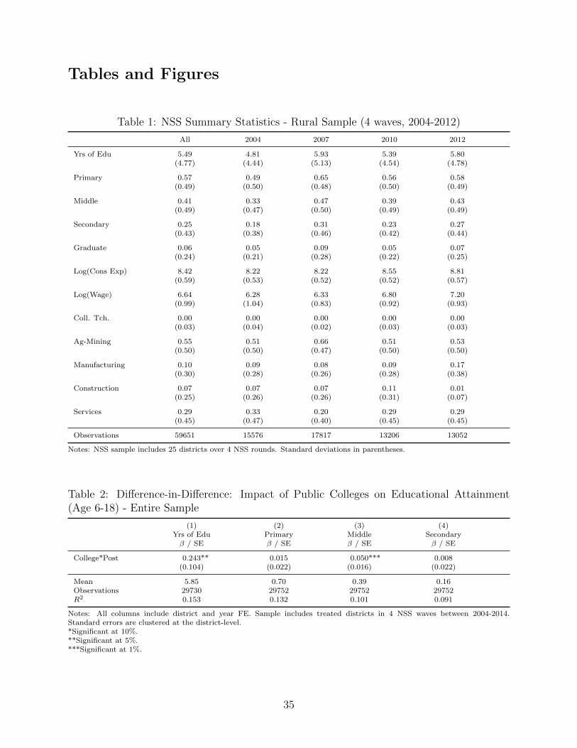
Tables and Figures

Table 1: NSS Summary Statistics - Rural Sample (4 waves, 2004-2012)

All 2004 2007 2010 2012

Yrs of Edu 5.49 4.81 5.93 5.39 5.80(4.77) (4.44) (5.13) (4.54) (4.78)

Primary 0.57 0.49 0.65 0.56 0.58(0.49) (0.50) (0.48) (0.50) (0.49)

Middle 0.41 0.33 0.47 0.39 0.43(0.49) (0.47) (0.50) (0.49) (0.49)

Secondary 0.25 0.18 0.31 0.23 0.27(0.43) (0.38) (0.46) (0.42) (0.44)

Graduate 0.06 0.05 0.09 0.05 0.07(0.24) (0.21) (0.28) (0.22) (0.25)

Log(Cons Exp) 8.42 8.22 8.22 8.55 8.81(0.59) (0.53) (0.52) (0.52) (0.57)

Log(Wage) 6.64 6.28 6.33 6.80 7.20(0.99) (1.04) (0.83) (0.92) (0.93)

Coll. Tch. 0.00 0.00 0.00 0.00 0.00(0.03) (0.04) (0.02) (0.03) (0.03)

Ag-Mining 0.55 0.51 0.66 0.51 0.53(0.50) (0.50) (0.47) (0.50) (0.50)

Manufacturing 0.10 0.09 0.08 0.09 0.17(0.30) (0.28) (0.26) (0.28) (0.38)

Construction 0.07 0.07 0.07 0.11 0.01(0.25) (0.26) (0.26) (0.31) (0.07)

Services 0.29 0.33 0.20 0.29 0.29(0.45) (0.47) (0.40) (0.45) (0.45)

Observations 59651 15576 17817 13206 13052

Notes: NSS sample includes 25 districts over 4 NSS rounds. Standard deviations in parentheses.

Table 2: Difference-in-Difference: Impact of Public Colleges on Educational Attainment(Age 6-18) - Entire Sample

(1) (2) (3) (4)Yrs of Edu Primary Middle Secondaryβ / SE β / SE β / SE β / SE

College*Post 0.243** 0.015 0.050*** 0.008(0.104) (0.022) (0.016) (0.022)

Mean 5.85 0.70 0.39 0.16Observations 29730 29752 29752 29752R2 0.153 0.132 0.101 0.091

Notes: All columns include district and year FE. Sample includes treated districts in 4 NSS waves between 2004-2014.Standard errors are clustered at the district-level.*Significant at 10%.**Significant at 5%.***Significant at 1%.

35

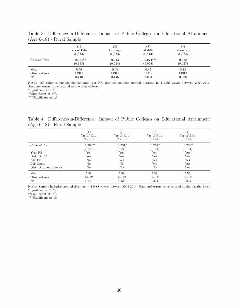
Table 3: Difference-in-Difference: Impact of Public Colleges on Educational Attainment(Age 6-18) - Rural Sample

(1) (2) (3) (4)Yrs of Edu Primary Middle Secondaryβ / SE β / SE β / SE β / SE

College*Post 0.304** 0.013 0.074*** 0.022(0.143) (0.024) (0.024) (0.027)

Mean 5.59 0.68 0.35 0.13Observations 14912 14919 14919 14919R2 0.140 0.146 0.093 0.080

Notes: All columns include district and year FE. Sample includes treated districts in 4 NSS waves between 2004-2014.Standard errors are clustered at the district-level.*Significant at 10%.**Significant at 5%.***Significant at 1%.

Table 4: Difference-in-Difference: Impact of Public Colleges on Educational Attainment(Age 6-18) - Rural Sample

(1) (2) (3) (4)Yrs of Edu Yrs of Edu Yrs of Edu Yrs of Eduβ / SE β / SE β / SE β / SE

College*Post 0.304** 0.231* 0.251* 0.290*(0.143) (0.133) (0.141) (0.151)

Year FE Yes Yes Yes YesDistrict FE Yes Yes Yes YesAge FE No Yes Yes YesLog Cons. No No Yes YesDistrict Linear Trends. No No No Yes

Mean 5.59 5.59 5.59 5.59Observations 14912 14912 14912 14912R2 0.140 0.525 0.531 0.532

Notes: Sample includes treated districts in 4 NSS waves between 2004-2014. Standard errors are clustered at the district-level.*Significant at 10%.**Significant at 5%.***Significant at 1%.

36

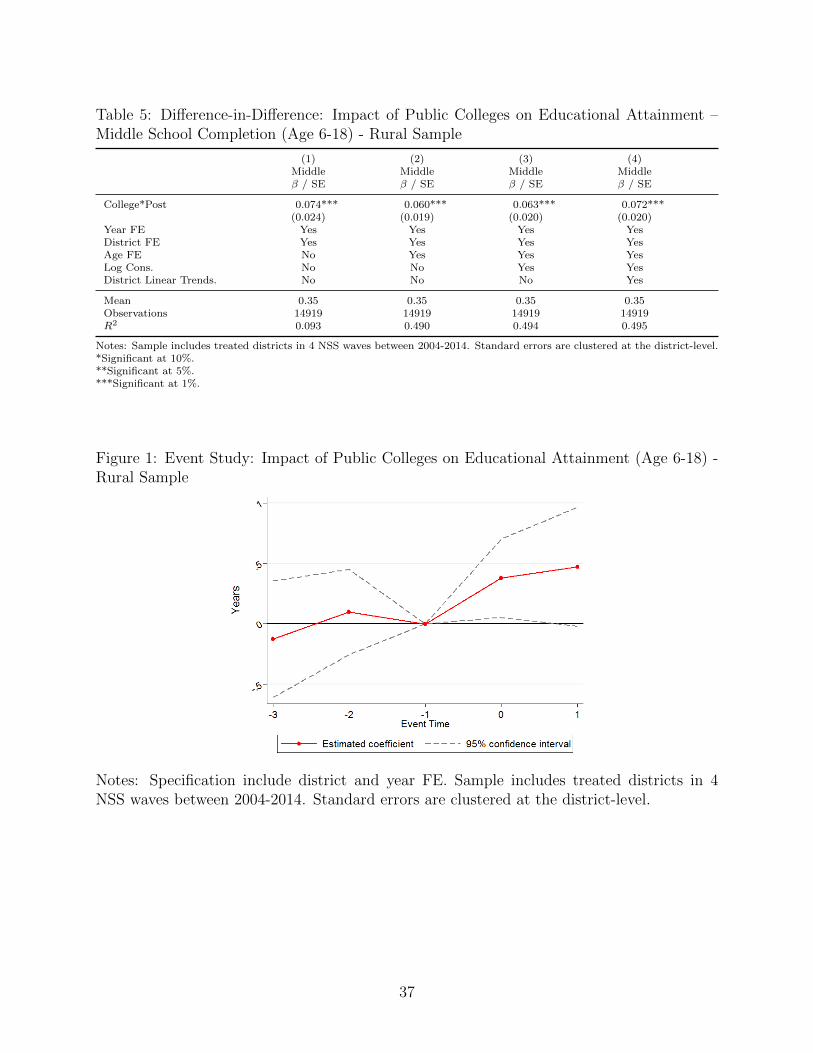
Table 5: Difference-in-Difference: Impact of Public Colleges on Educational Attainment –Middle School Completion (Age 6-18) - Rural Sample

(1) (2) (3) (4)Middle Middle Middle Middleβ / SE β / SE β / SE β / SE

College*Post 0.074*** 0.060*** 0.063*** 0.072***(0.024) (0.019) (0.020) (0.020)

Year FE Yes Yes Yes YesDistrict FE Yes Yes Yes YesAge FE No Yes Yes YesLog Cons. No No Yes YesDistrict Linear Trends. No No No Yes

Mean 0.35 0.35 0.35 0.35Observations 14919 14919 14919 14919R2 0.093 0.490 0.494 0.495

Notes: Sample includes treated districts in 4 NSS waves between 2004-2014. Standard errors are clustered at the district-level.*Significant at 10%.**Significant at 5%.***Significant at 1%.

Figure 1: Event Study: Impact of Public Colleges on Educational Attainment (Age 6-18) -Rural Sample

Notes: Specification include district and year FE. Sample includes treated districts in 4NSS waves between 2004-2014. Standard errors are clustered at the district-level.

37

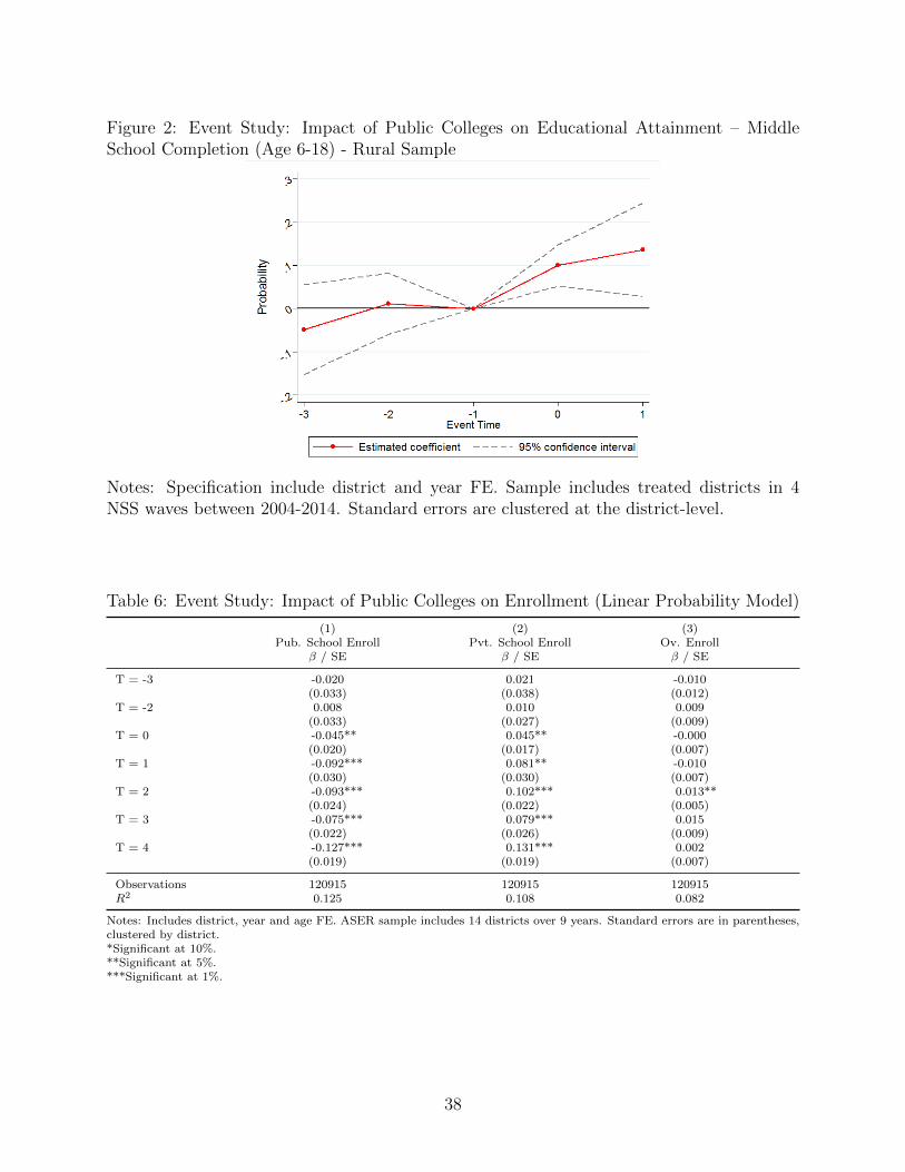
Figure 2: Event Study: Impact of Public Colleges on Educational Attainment – MiddleSchool Completion (Age 6-18) - Rural Sample

Notes: Specification include district and year FE. Sample includes treated districts in 4NSS waves between 2004-2014. Standard errors are clustered at the district-level.

Table 6: Event Study: Impact of Public Colleges on Enrollment (Linear Probability Model)

(1) (2) (3)Pub. School Enroll Pvt. School Enroll Ov. Enroll

β / SE β / SE β / SE

T = -3 -0.020 0.021 -0.010(0.033) (0.038) (0.012)

T = -2 0.008 0.010 0.009(0.033) (0.027) (0.009)

T = 0 -0.045** 0.045** -0.000(0.020) (0.017) (0.007)

T = 1 -0.092*** 0.081** -0.010(0.030) (0.030) (0.007)

T = 2 -0.093*** 0.102*** 0.013**(0.024) (0.022) (0.005)

T = 3 -0.075*** 0.079*** 0.015(0.022) (0.026) (0.009)

T = 4 -0.127*** 0.131*** 0.002(0.019) (0.019) (0.007)

Observations 120915 120915 120915R2 0.125 0.108 0.082

Notes: Includes district, year and age FE. ASER sample includes 14 districts over 9 years. Standard errors are in parentheses,clustered by district.*Significant at 10%.**Significant at 5%.***Significant at 1%.

38

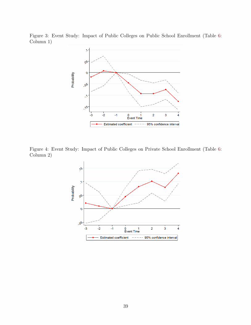
Figure 3: Event Study: Impact of Public Colleges on Public School Enrollment (Table 6:Column 1)

Figure 4: Event Study: Impact of Public Colleges on Private School Enrollment (Table 6:Column 2)

39

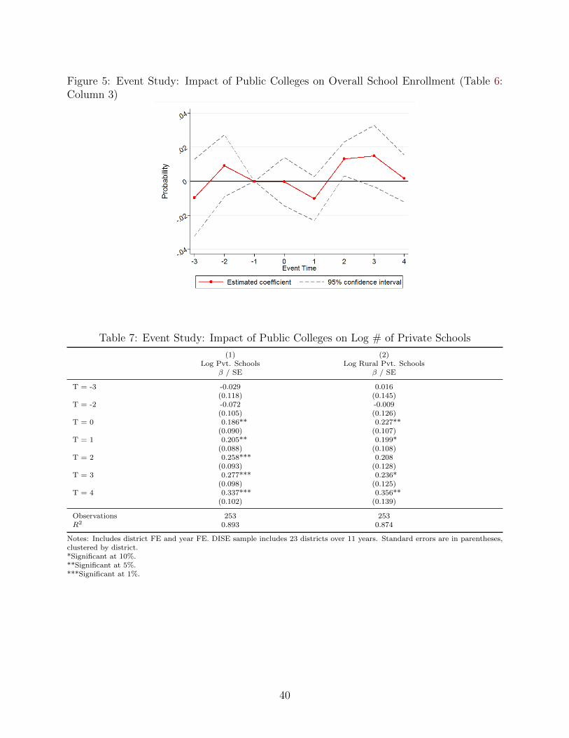
Figure 5: Event Study: Impact of Public Colleges on Overall School Enrollment (Table 6:Column 3)

Table 7: Event Study: Impact of Public Colleges on Log # of Private Schools

(1) (2)Log Pvt. Schools Log Rural Pvt. Schools

β / SE β / SE

T = -3 -0.029 0.016(0.118) (0.145)

T = -2 -0.072 -0.009(0.105) (0.126)

T = 0 0.186** 0.227**(0.090) (0.107)

T = 1 0.205** 0.199*(0.088) (0.108)

T = 2 0.258*** 0.208(0.093) (0.128)

T = 3 0.277*** 0.236*(0.098) (0.125)

T = 4 0.337*** 0.356**(0.102) (0.139)

Observations 253 253R2 0.893 0.874

Notes: Includes district FE and year FE. DISE sample includes 23 districts over 11 years. Standard errors are in parentheses,clustered by district.*Significant at 10%.**Significant at 5%.***Significant at 1%.

40

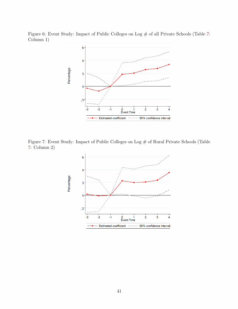
Figure 6: Event Study: Impact of Public Colleges on Log # of all Private Schools (Table 7:Column 1)

Figure 7: Event Study: Impact of Public Colleges on Log # of Rural Private Schools (Table7: Column 2)

41

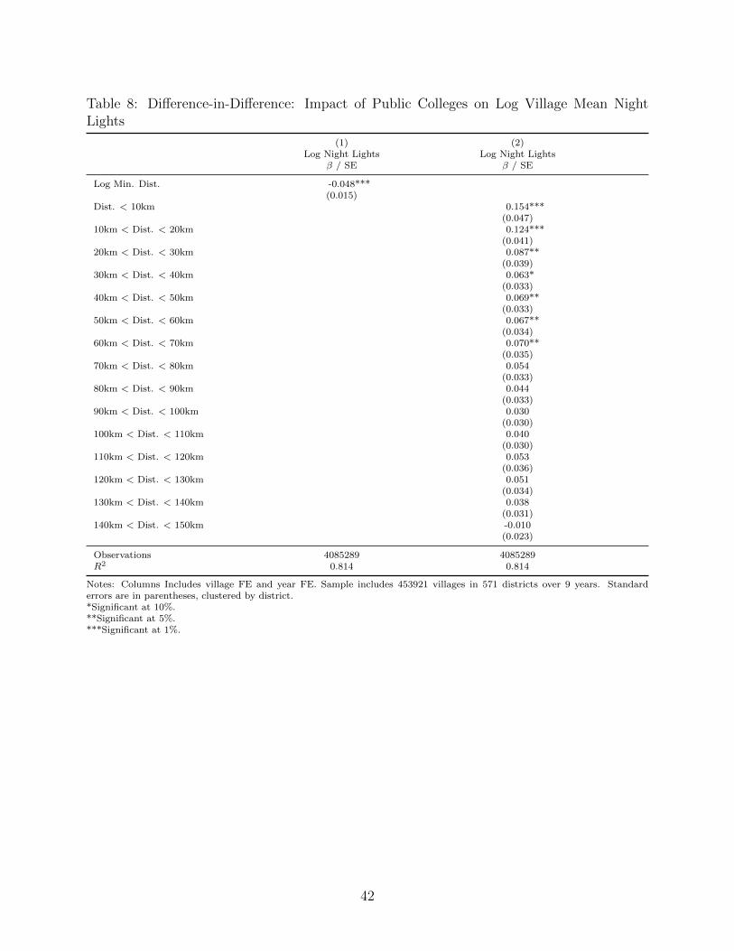
Table 8: Difference-in-Difference: Impact of Public Colleges on Log Village Mean NightLights

(1) (2)Log Night Lights Log Night Lights

β / SE β / SE

Log Min. Dist. -0.048***(0.015)

Dist. < 10km 0.154***(0.047)

10km < Dist. < 20km 0.124***(0.041)

20km < Dist. < 30km 0.087**(0.039)

30km < Dist. < 40km 0.063*(0.033)

40km < Dist. < 50km 0.069**(0.033)

50km < Dist. < 60km 0.067**(0.034)

60km < Dist. < 70km 0.070**(0.035)

70km < Dist. < 80km 0.054(0.033)

80km < Dist. < 90km 0.044(0.033)

90km < Dist. < 100km 0.030(0.030)

100km < Dist. < 110km 0.040(0.030)

110km < Dist. < 120km 0.053(0.036)

120km < Dist. < 130km 0.051(0.034)

130km < Dist. < 140km 0.038(0.031)

140km < Dist. < 150km -0.010(0.023)

Observations 4085289 4085289R2 0.814 0.814

Notes: Columns Includes village FE and year FE. Sample includes 453921 villages in 571 districts over 9 years. Standarderrors are in parentheses, clustered by district.*Significant at 10%.**Significant at 5%.***Significant at 1%.

42

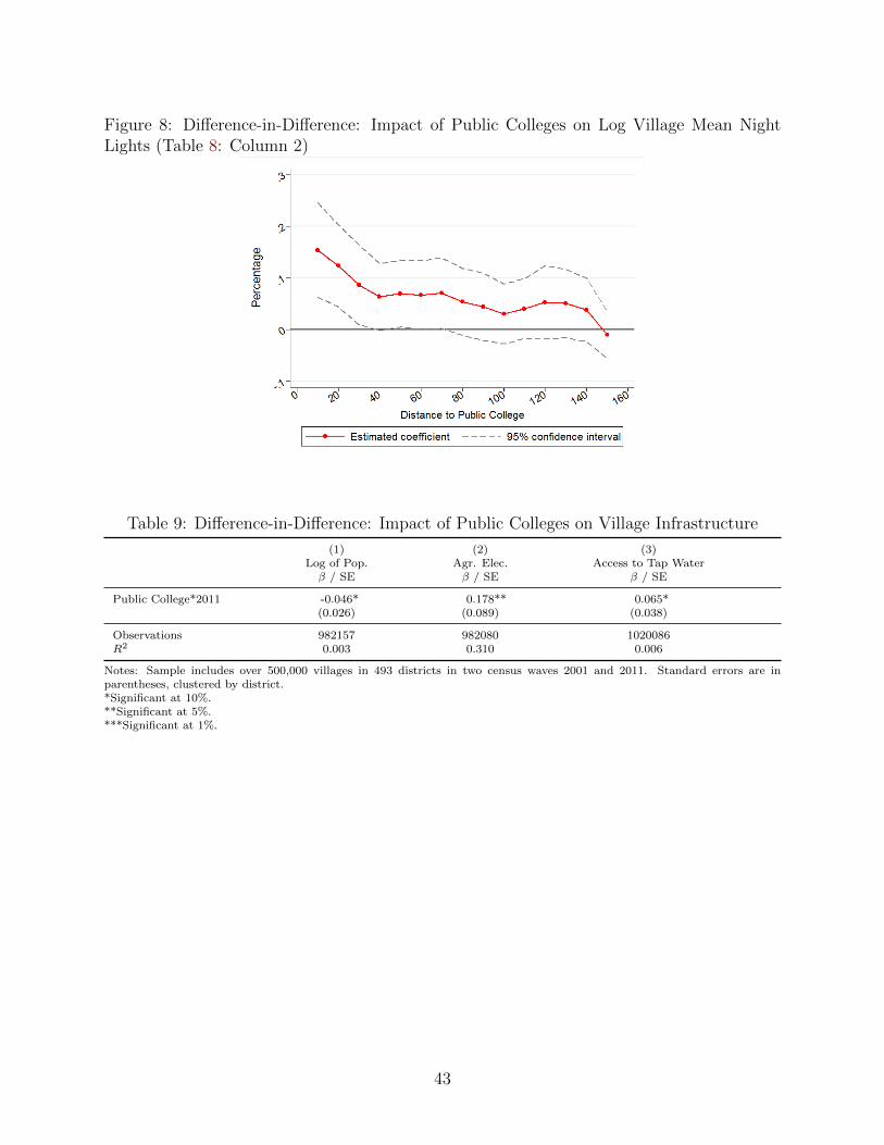
Figure 8: Difference-in-Difference: Impact of Public Colleges on Log Village Mean NightLights (Table 8: Column 2)

Table 9: Difference-in-Difference: Impact of Public Colleges on Village Infrastructure

(1) (2) (3)Log of Pop. Agr. Elec. Access to Tap Waterβ / SE β / SE β / SE

Public College*2011 -0.046* 0.178** 0.065*(0.026) (0.089) (0.038)

Observations 982157 982080 1020086R2 0.003 0.310 0.006

Notes: Sample includes over 500,000 villages in 493 districts in two census waves 2001 and 2011. Standard errors are inparentheses, clustered by district.*Significant at 10%.**Significant at 5%.***Significant at 1%.

43

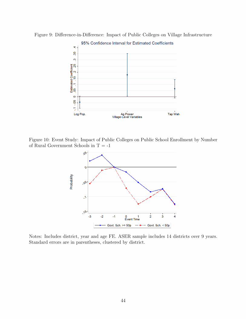
Figure 9: Difference-in-Difference: Impact of Public Colleges on Village Infrastructure

Figure 10: Event Study: Impact of Public Colleges on Public School Enrollment by Numberof Rural Government Schools in T = -1

Notes: Includes district, year and age FE. ASER sample includes 14 districts over 9 years.Standard errors are in parentheses, clustered by district.

44

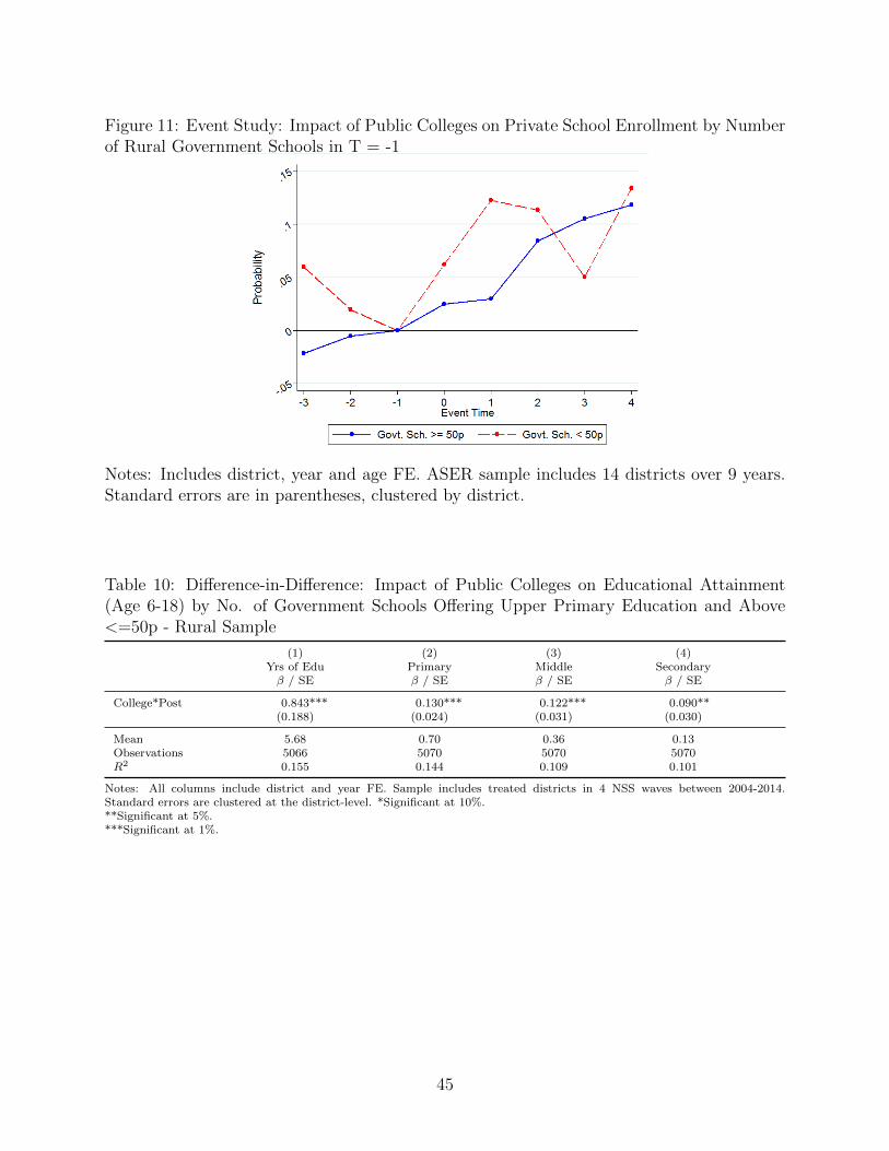
Figure 11: Event Study: Impact of Public Colleges on Private School Enrollment by Numberof Rural Government Schools in T = -1

Notes: Includes district, year and age FE. ASER sample includes 14 districts over 9 years.Standard errors are in parentheses, clustered by district.

Table 10: Difference-in-Difference: Impact of Public Colleges on Educational Attainment(Age 6-18) by No. of Government Schools Offering Upper Primary Education and Above<=50p - Rural Sample

(1) (2) (3) (4)Yrs of Edu Primary Middle Secondaryβ / SE β / SE β / SE β / SE

College*Post 0.843*** 0.130*** 0.122*** 0.090**(0.188) (0.024) (0.031) (0.030)

Mean 5.68 0.70 0.36 0.13Observations 5066 5070 5070 5070R2 0.155 0.144 0.109 0.101

Notes: All columns include district and year FE. Sample includes treated districts in 4 NSS waves between 2004-2014.Standard errors are clustered at the district-level. *Significant at 10%.**Significant at 5%.***Significant at 1%.

45

Table 11: Difference-in-Difference: Impact of Public Colleges on Educational Attainment(Age 6-18) by No. of Government Schools Offering Upper Primary Education and Above>50p - Rural Sample

(1) (2) (3) (4)Yrs of Edu Primary Middle Secondaryβ / SE β / SE β / SE β / SE

College*Post 0.372 0.004 0.080* 0.048*(0.236) (0.040) (0.038) (0.026)

Mean 5.46 0.65 0.34 0.13Observations 7635 7637 7637 7637R2 0.130 0.153 0.076 0.074

Notes: All columns include district and year FE. Sample includes treated districts in 4 NSS waves between 2004-2014.Standard errors are clustered at the district-level. *Significant at 10%.**Significant at 5%.***Significant at 1%.

Figure 12: Proximity to Elite Public College and Presence of Public vs Private School in2011

Notes: Includes district FE. Sample includes over 500,000 villages in 493 districts in 2011census wave. Standard errors are in parentheses, clustered by district.

46

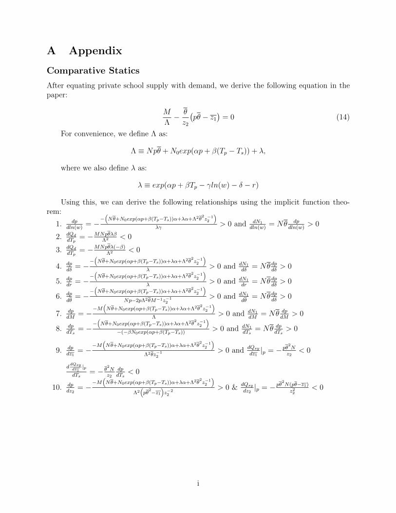
A Appendix

Comparative Statics

After equating private school supply with demand, we derive the following equation in thepaper:

M

Λ− θ

z2

(pθ − z1

)= 0 (14)

For convenience, we define Λ as:

Λ ≡ Npθ +N0exp(αp+ β(Tp − Ts)) + λ,

where we also define λ as:

λ ≡ exp(αp+ βTp − γln(w)− δ − r)

Using this, we can derive the following relationships using the implicit function theo-rem:

1. dpdln(w)

= −−(Nθ+N0exp(αp+β(Tp−Ts))α+λα+Λ2θ

2z−12

)λγ

> 0 and dN1

dln(w)= Nθ dp

dln(w)> 0

2. dQd

dTp= −MNpθλβ

Λ2 < 0

3. dQd

dTp= −MNpθλ(−β)

Λ2 < 0

4. dpdδ

= −−(Nθ+N0exp(αp+β(Tp−Ts))α+λα+Λ2θ

2z−12

)λ

> 0 and dN1

dδ= Nθ dp

dδ> 0

5. dpdr

= −−(Nθ+N0exp(αp+β(Tp−Ts))α+λα+Λ2θ

2z−12

)λ

> 0 and dN1

dr= Nθ dp

dδ> 0

6. dp

dθ= −

−(Nθ+N0exp(αp+β(Tp−Ts))α+λα+Λ2θ

2z−12

)Np−2pΛ2θM−1z−1

2

> 0 and dN1

dθ= Nθ dp

dδ> 0

7. dpdM

= −−M

(Nθ+N0exp(αp+β(Tp−Ts))α+λα+Λ2θ

2z−12

)Λ

> 0 and dN1

dM= Nθ dp

dM> 0

8. dpdTs

= −−(Nθ+N0exp(αp+β(Tp−Ts))α+λα+Λ2θ

2z−12

)−(−βN0exp(αp+β(Tp−Ts))

> 0 and dN1

dTs= Nθ dp

dTs> 0

9. dpdz1

= −−M

(Nθ+N0exp(αp+β(Tp−Ts))α+λα+Λ2θ

2z−12

)Λ2θz−1

2

> 0 and dQsy

dz1|p = −pθ

2N

z2< 0

ddQsydz1|p

dTs= − θ

2Nz2

dpdTs

< 0

10. dpdz2

= −−M

(Nθ+N0exp(αp+β(Tp−Ts))α+λα+Λ2θ

2z−12

)Λ2

(pθ

2−z1)z−22

> 0 & dQsy

dz2|p = −pθ

2N(pθ−z1)

z22< 0

i

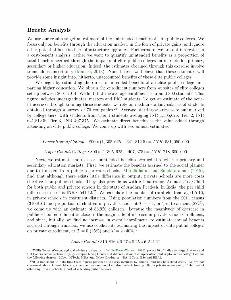
Benefit Analysis

We use our results to get an estimate of the unintended benefits of elite public colleges. Wefocus only on benefits through the education market, in the form of private gains, and ignoreother potential benefits like infrastructure upgrades. Furthermore, we are not interested ina cost-benefit analysis, rather we want to quantify unintended benefits as a proportion oftotal benefits accrued through the impacts of elite public colleges on markets for primary,secondary or higher education. Indeed, the estimates obtained through this exercise involvetremendous uncertainty (Manski, 2013). Nonetheless, we believe that these estimates willprovide some insight into, hitherto, unaccounted benefits of these elite public colleges.

We begin by estimating the direct or intended benefits of an elite public college im-parting higher education. We obtain the enrollment numbers from websites of elite collegesset-up between 2004-2014. We find that the average enrollment is around 800 students. Thisfigure includes undergraduates, masters and PhD students. To get an estimate of the bene-fit accrued through training these students, we rely on median starting-salaries of studentsobtained through a survey of 70 companies.24 Average starting-salaries were summarizedby college tiers, with students from Tier 1 students averaging INR 1,305,625; Tier 2, INR641,812.5; Tier 3, INR 407,375. We estimate direct benefits as the value added throughattending an elite public college. We come up with two annual estimates:

LowerBound/College : 800 ∗ (1, 305, 625− 641, 812.5) = INR 531, 050, 000

UpperBound/College : 800 ∗ (1, 305, 625− 407, 375) = INR 718, 600, 000

Next, we estimate indirect, or unintended benefits accrued through the primary andsecondary education markets. First, we estimate the benefits accrued to the social plannerdue to transfers from public to private schools. Muralidharan and Sundararaman (2015),find that although there exists little difference in output, private schools are more costseffective than public schools. They also provide us with estimates for ‘Annual Cost/Childfor both public and private schools in the state of Andhra Pradesh, in India; the per childdifference in cost is INR 6,541.12.25 We calculate the number of rural children, aged 5-16,in private schools in treatment districts. Using population numbers from the 2011 census(310,816) and proportion of children in private schools at T = −1, or ‘pre-treatment (27%),we come up with an estimate of 83,920 children. Because the magnitude of decrease inpublic school enrollment is close to the magnitude of increase in private school enrollment,and since, initially, we find no increase in overall enrollment, to estimate annual benefitsaccrued through transfers, we use coefficients estimating the impact of elite public collegeson private enrollment, at T = 0 (25%) and T = 2 (40%):

LowerBound : 310, 816 ∗ 0.27 ∗ 0.25 ∗ 6, 541.12

24Willis Tower Watson, a global advisory company, in Willis-Tower-Watson (2016), polled 70 of Indias top organizations andHR leaders across sectors to gauge campus hiring trends and differentiation of compensation philosophy across college tiers forthe following degrees BTech, MTech, MBA and Other Graduates (BA, BCom, BSc and BBA).

25It is important to note that these figures pertain to the cost incurred by schools, and not household costs. We are notconcerned about household costs, since, as per our model children switch from public to private schools only if the cost ofattending private schools < cost of attending public schools.

ii

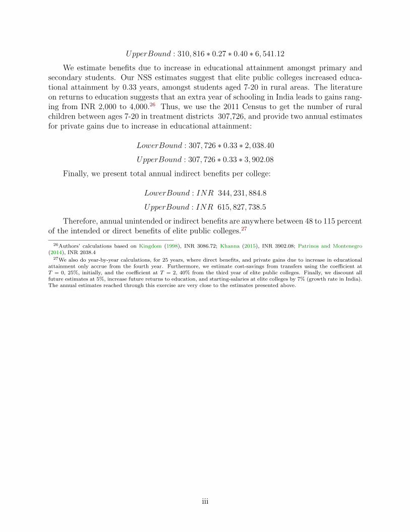
UpperBound : 310, 816 ∗ 0.27 ∗ 0.40 ∗ 6, 541.12

We estimate benefits due to increase in educational attainment amongst primary andsecondary students. Our NSS estimates suggest that elite public colleges increased educa-tional attainment by 0.33 years, amongst students aged 7-20 in rural areas. The literatureon returns to education suggests that an extra year of schooling in India leads to gains rang-ing from INR 2,000 to 4,000.26 Thus, we use the 2011 Census to get the number of ruralchildren between ages 7-20 in treatment districts 307,726, and provide two annual estimatesfor private gains due to increase in educational attainment:

LowerBound : 307, 726 ∗ 0.33 ∗ 2, 038.40

UpperBound : 307, 726 ∗ 0.33 ∗ 3, 902.08

Finally, we present total annual indirect benefits per college:

LowerBound : INR 344, 231, 884.8

UpperBound : INR 615, 827, 738.5

Therefore, annual unintended or indirect benefits are anywhere between 48 to 115 percentof the intended or direct benefits of elite public colleges.27

26Authors’ calculations based on Kingdom (1998), INR 3086.72; Khanna (2015), INR 3902.08; Patrinos and Montenegro(2014), INR 2038.4

27We also do year-by-year calculations, for 25 years, where direct benefits, and private gains due to increase in educationalattainment only accrue from the fourth year. Furthermore, we estimate cost-savings from transfers using the coefficient atT = 0, 25%, initially, and the coefficient at T = 2, 40% from the third year of elite public colleges. Finally, we discount allfuture estimates at 5%, increase future returns to education, and starting-salaries at elite colleges by 7% (growth rate in India).The annual estimates reached through this exercise are very close to the estimates presented above.

iii

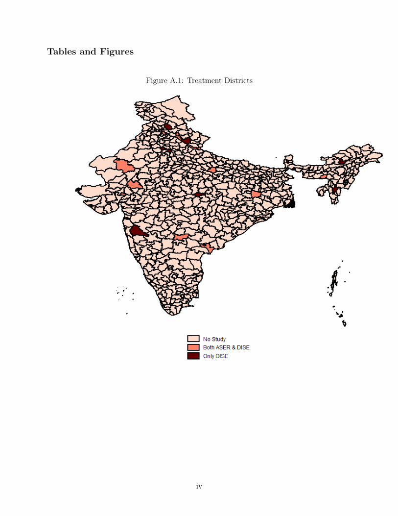
Tables and Figures

Figure A.1: Treatment Districts

iv

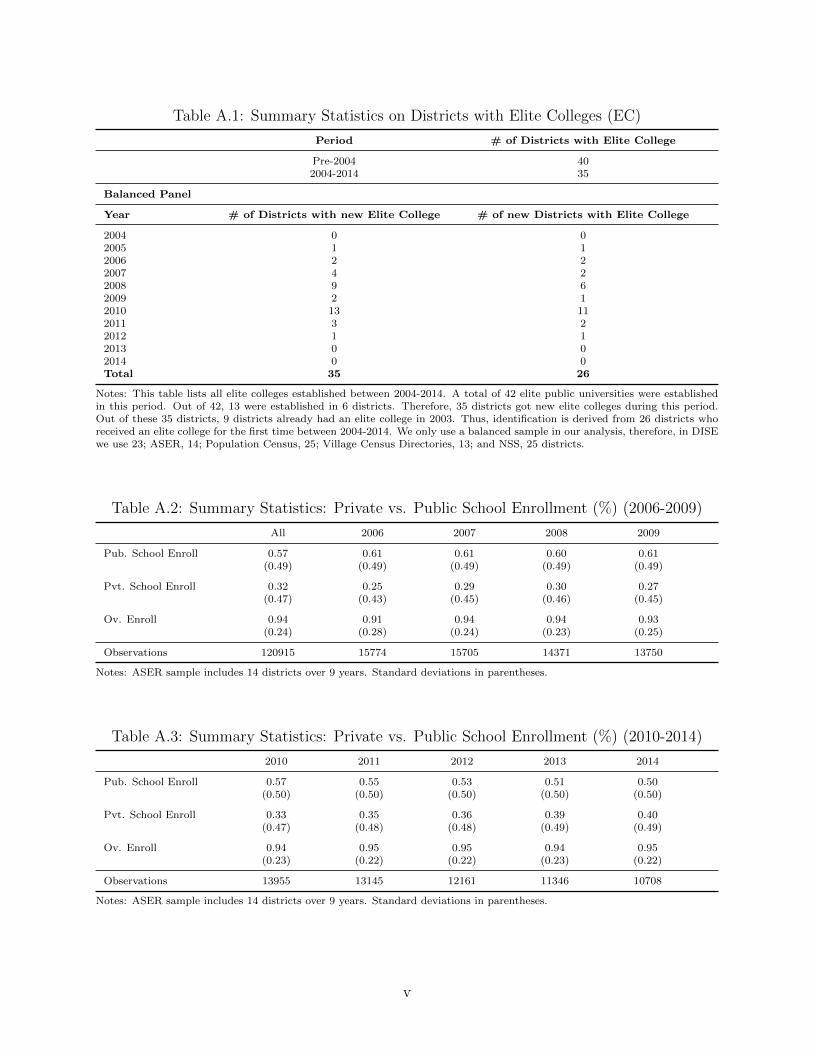
Table A.1: Summary Statistics on Districts with Elite Colleges (EC)

Period # of Districts with Elite College

Pre-2004 402004-2014 35

Balanced Panel

Year # of Districts with new Elite College # of new Districts with Elite College

2004 0 02005 1 12006 2 22007 4 22008 9 62009 2 12010 13 112011 3 22012 1 12013 0 02014 0 0Total 35 26

Notes: This table lists all elite colleges established between 2004-2014. A total of 42 elite public universities were establishedin this period. Out of 42, 13 were established in 6 districts. Therefore, 35 districts got new elite colleges during this period.Out of these 35 districts, 9 districts already had an elite college in 2003. Thus, identification is derived from 26 districts whoreceived an elite college for the first time between 2004-2014. We only use a balanced sample in our analysis, therefore, in DISEwe use 23; ASER, 14; Population Census, 25; Village Census Directories, 13; and NSS, 25 districts.

Table A.2: Summary Statistics: Private vs. Public School Enrollment (%) (2006-2009)

All 2006 2007 2008 2009

Pub. School Enroll 0.57 0.61 0.61 0.60 0.61(0.49) (0.49) (0.49) (0.49) (0.49)

Pvt. School Enroll 0.32 0.25 0.29 0.30 0.27(0.47) (0.43) (0.45) (0.46) (0.45)

Ov. Enroll 0.94 0.91 0.94 0.94 0.93(0.24) (0.28) (0.24) (0.23) (0.25)

Observations 120915 15774 15705 14371 13750

Notes: ASER sample includes 14 districts over 9 years. Standard deviations in parentheses.

Table A.3: Summary Statistics: Private vs. Public School Enrollment (%) (2010-2014)

2010 2011 2012 2013 2014

Pub. School Enroll 0.57 0.55 0.53 0.51 0.50(0.50) (0.50) (0.50) (0.50) (0.50)

Pvt. School Enroll 0.33 0.35 0.36 0.39 0.40(0.47) (0.48) (0.48) (0.49) (0.49)

Ov. Enroll 0.94 0.95 0.95 0.94 0.95(0.23) (0.22) (0.22) (0.23) (0.22)

Observations 13955 13145 12161 11346 10708

Notes: ASER sample includes 14 districts over 9 years. Standard deviations in parentheses.

v

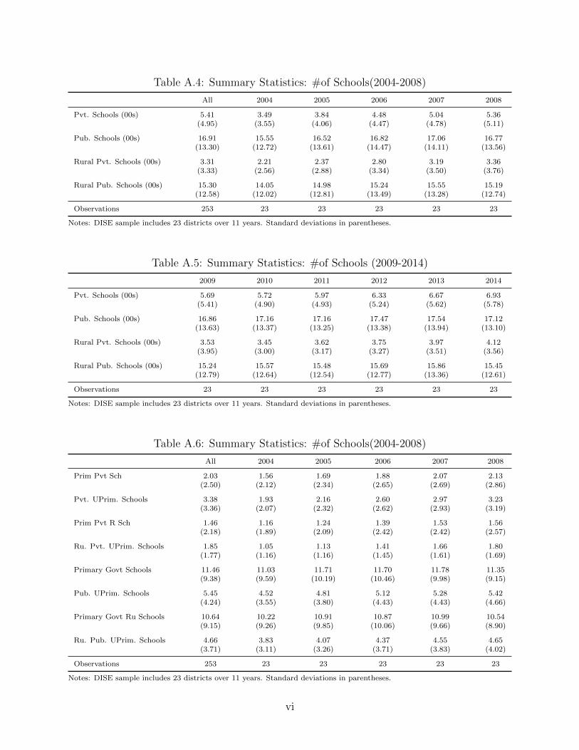
Table A.4: Summary Statistics: #of Schools(2004-2008)

All 2004 2005 2006 2007 2008

Pvt. Schools (00s) 5.41 3.49 3.84 4.48 5.04 5.36(4.95) (3.55) (4.06) (4.47) (4.78) (5.11)

Pub. Schools (00s) 16.91 15.55 16.52 16.82 17.06 16.77(13.30) (12.72) (13.61) (14.47) (14.11) (13.56)

Rural Pvt. Schools (00s) 3.31 2.21 2.37 2.80 3.19 3.36(3.33) (2.56) (2.88) (3.34) (3.50) (3.76)

Rural Pub. Schools (00s) 15.30 14.05 14.98 15.24 15.55 15.19(12.58) (12.02) (12.81) (13.49) (13.28) (12.74)

Observations 253 23 23 23 23 23

Notes: DISE sample includes 23 districts over 11 years. Standard deviations in parentheses.

Table A.5: Summary Statistics: #of Schools (2009-2014)

2009 2010 2011 2012 2013 2014

Pvt. Schools (00s) 5.69 5.72 5.97 6.33 6.67 6.93(5.41) (4.90) (4.93) (5.24) (5.62) (5.78)

Pub. Schools (00s) 16.86 17.16 17.16 17.47 17.54 17.12(13.63) (13.37) (13.25) (13.38) (13.94) (13.10)

Rural Pvt. Schools (00s) 3.53 3.45 3.62 3.75 3.97 4.12(3.95) (3.00) (3.17) (3.27) (3.51) (3.56)

Rural Pub. Schools (00s) 15.24 15.57 15.48 15.69 15.86 15.45(12.79) (12.64) (12.54) (12.77) (13.36) (12.61)

Observations 23 23 23 23 23 23

Notes: DISE sample includes 23 districts over 11 years. Standard deviations in parentheses.

Table A.6: Summary Statistics: #of Schools(2004-2008)

All 2004 2005 2006 2007 2008

Prim Pvt Sch 2.03 1.56 1.69 1.88 2.07 2.13(2.50) (2.12) (2.34) (2.65) (2.69) (2.86)

Pvt. UPrim. Schools 3.38 1.93 2.16 2.60 2.97 3.23(3.36) (2.07) (2.32) (2.62) (2.93) (3.19)

Prim Pvt R Sch 1.46 1.16 1.24 1.39 1.53 1.56(2.18) (1.89) (2.09) (2.42) (2.42) (2.57)

Ru. Pvt. UPrim. Schools 1.85 1.05 1.13 1.41 1.66 1.80(1.77) (1.16) (1.16) (1.45) (1.61) (1.69)

Primary Govt Schools 11.46 11.03 11.71 11.70 11.78 11.35(9.38) (9.59) (10.19) (10.46) (9.98) (9.15)

Pub. UPrim. Schools 5.45 4.52 4.81 5.12 5.28 5.42(4.24) (3.55) (3.80) (4.43) (4.43) (4.66)

Primary Govt Ru Schools 10.64 10.22 10.91 10.87 10.99 10.54(9.15) (9.26) (9.85) (10.06) (9.66) (8.90)

Ru. Pub. UPrim. Schools 4.66 3.83 4.07 4.37 4.55 4.65(3.71) (3.11) (3.26) (3.71) (3.83) (4.02)

Observations 253 23 23 23 23 23

Notes: DISE sample includes 23 districts over 11 years. Standard deviations in parentheses.

vi

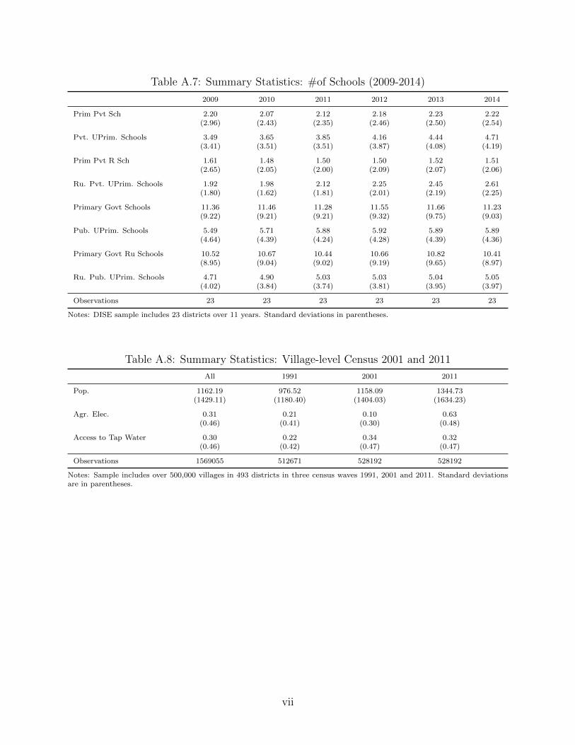
Table A.7: Summary Statistics: #of Schools (2009-2014)

2009 2010 2011 2012 2013 2014

Prim Pvt Sch 2.20 2.07 2.12 2.18 2.23 2.22(2.96) (2.43) (2.35) (2.46) (2.50) (2.54)

Pvt. UPrim. Schools 3.49 3.65 3.85 4.16 4.44 4.71(3.41) (3.51) (3.51) (3.87) (4.08) (4.19)

Prim Pvt R Sch 1.61 1.48 1.50 1.50 1.52 1.51(2.65) (2.05) (2.00) (2.09) (2.07) (2.06)

Ru. Pvt. UPrim. Schools 1.92 1.98 2.12 2.25 2.45 2.61(1.80) (1.62) (1.81) (2.01) (2.19) (2.25)

Primary Govt Schools 11.36 11.46 11.28 11.55 11.66 11.23(9.22) (9.21) (9.21) (9.32) (9.75) (9.03)

Pub. UPrim. Schools 5.49 5.71 5.88 5.92 5.89 5.89(4.64) (4.39) (4.24) (4.28) (4.39) (4.36)

Primary Govt Ru Schools 10.52 10.67 10.44 10.66 10.82 10.41(8.95) (9.04) (9.02) (9.19) (9.65) (8.97)

Ru. Pub. UPrim. Schools 4.71 4.90 5.03 5.03 5.04 5.05(4.02) (3.84) (3.74) (3.81) (3.95) (3.97)

Observations 23 23 23 23 23 23

Notes: DISE sample includes 23 districts over 11 years. Standard deviations in parentheses.

Table A.8: Summary Statistics: Village-level Census 2001 and 2011

All 1991 2001 2011

Pop. 1162.19 976.52 1158.09 1344.73(1429.11) (1180.40) (1404.03) (1634.23)

Agr. Elec. 0.31 0.21 0.10 0.63(0.46) (0.41) (0.30) (0.48)

Access to Tap Water 0.30 0.22 0.34 0.32(0.46) (0.42) (0.47) (0.47)

Observations 1569055 512671 528192 528192

Notes: Sample includes over 500,000 villages in 493 districts in three census waves 1991, 2001 and 2011. Standard deviationsare in parentheses.

vii

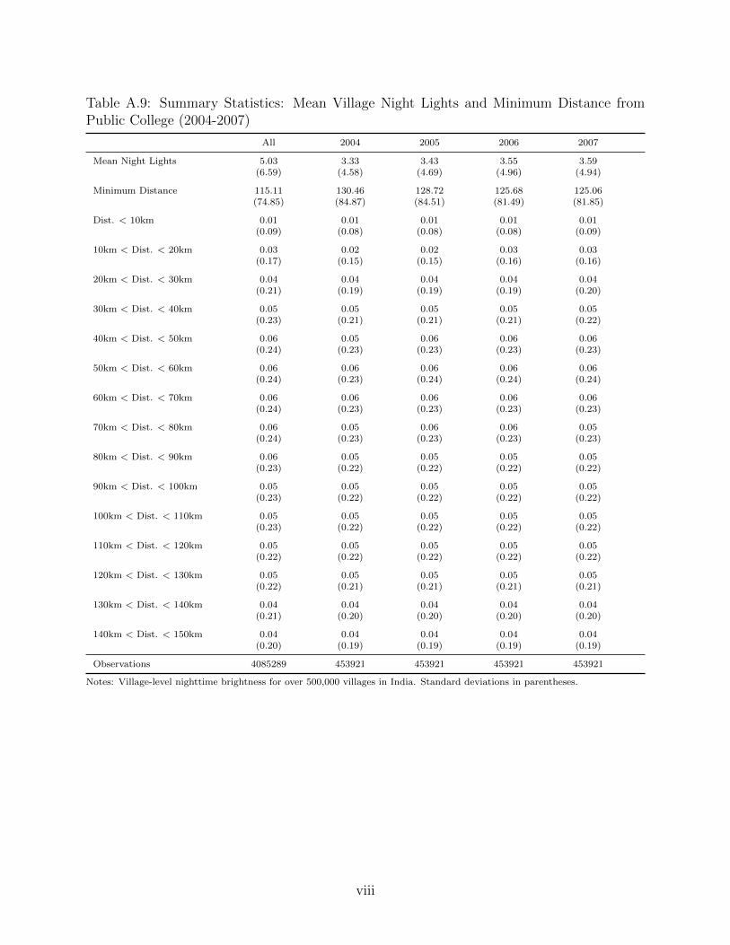
Table A.9: Summary Statistics: Mean Village Night Lights and Minimum Distance fromPublic College (2004-2007)

All 2004 2005 2006 2007

Mean Night Lights 5.03 3.33 3.43 3.55 3.59(6.59) (4.58) (4.69) (4.96) (4.94)

Minimum Distance 115.11 130.46 128.72 125.68 125.06(74.85) (84.87) (84.51) (81.49) (81.85)

Dist. < 10km 0.01 0.01 0.01 0.01 0.01(0.09) (0.08) (0.08) (0.08) (0.09)

10km < Dist. < 20km 0.03 0.02 0.02 0.03 0.03(0.17) (0.15) (0.15) (0.16) (0.16)

20km < Dist. < 30km 0.04 0.04 0.04 0.04 0.04(0.21) (0.19) (0.19) (0.19) (0.20)

30km < Dist. < 40km 0.05 0.05 0.05 0.05 0.05(0.23) (0.21) (0.21) (0.21) (0.22)

40km < Dist. < 50km 0.06 0.05 0.06 0.06 0.06(0.24) (0.23) (0.23) (0.23) (0.23)

50km < Dist. < 60km 0.06 0.06 0.06 0.06 0.06(0.24) (0.23) (0.24) (0.24) (0.24)

60km < Dist. < 70km 0.06 0.06 0.06 0.06 0.06(0.24) (0.23) (0.23) (0.23) (0.23)

70km < Dist. < 80km 0.06 0.05 0.06 0.06 0.05(0.24) (0.23) (0.23) (0.23) (0.23)

80km < Dist. < 90km 0.06 0.05 0.05 0.05 0.05(0.23) (0.22) (0.22) (0.22) (0.22)

90km < Dist. < 100km 0.05 0.05 0.05 0.05 0.05(0.23) (0.22) (0.22) (0.22) (0.22)

100km < Dist. < 110km 0.05 0.05 0.05 0.05 0.05(0.23) (0.22) (0.22) (0.22) (0.22)

110km < Dist. < 120km 0.05 0.05 0.05 0.05 0.05(0.22) (0.22) (0.22) (0.22) (0.22)

120km < Dist. < 130km 0.05 0.05 0.05 0.05 0.05(0.22) (0.21) (0.21) (0.21) (0.21)

130km < Dist. < 140km 0.04 0.04 0.04 0.04 0.04(0.21) (0.20) (0.20) (0.20) (0.20)

140km < Dist. < 150km 0.04 0.04 0.04 0.04 0.04(0.20) (0.19) (0.19) (0.19) (0.19)

Observations 4085289 453921 453921 453921 453921

Notes: Village-level nighttime brightness for over 500,000 villages in India. Standard deviations in parentheses.

viii

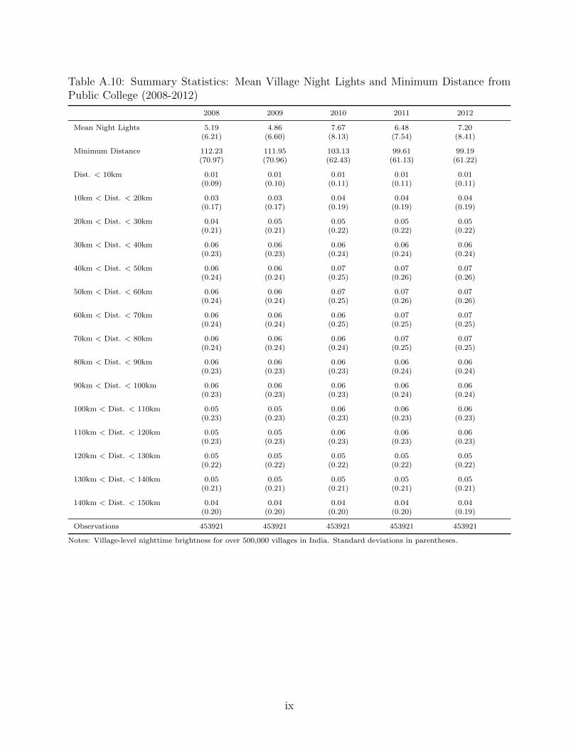
Table A.10: Summary Statistics: Mean Village Night Lights and Minimum Distance fromPublic College (2008-2012)

2008 2009 2010 2011 2012

Mean Night Lights 5.19 4.86 7.67 6.48 7.20(6.21) (6.60) (8.13) (7.54) (8.41)

Minimum Distance 112.23 111.95 103.13 99.61 99.19(70.97) (70.96) (62.43) (61.13) (61.22)

Dist. < 10km 0.01 0.01 0.01 0.01 0.01(0.09) (0.10) (0.11) (0.11) (0.11)

10km < Dist. < 20km 0.03 0.03 0.04 0.04 0.04(0.17) (0.17) (0.19) (0.19) (0.19)

20km < Dist. < 30km 0.04 0.05 0.05 0.05 0.05(0.21) (0.21) (0.22) (0.22) (0.22)

30km < Dist. < 40km 0.06 0.06 0.06 0.06 0.06(0.23) (0.23) (0.24) (0.24) (0.24)

40km < Dist. < 50km 0.06 0.06 0.07 0.07 0.07(0.24) (0.24) (0.25) (0.26) (0.26)

50km < Dist. < 60km 0.06 0.06 0.07 0.07 0.07(0.24) (0.24) (0.25) (0.26) (0.26)

60km < Dist. < 70km 0.06 0.06 0.06 0.07 0.07(0.24) (0.24) (0.25) (0.25) (0.25)

70km < Dist. < 80km 0.06 0.06 0.06 0.07 0.07(0.24) (0.24) (0.24) (0.25) (0.25)

80km < Dist. < 90km 0.06 0.06 0.06 0.06 0.06(0.23) (0.23) (0.23) (0.24) (0.24)

90km < Dist. < 100km 0.06 0.06 0.06 0.06 0.06(0.23) (0.23) (0.23) (0.24) (0.24)

100km < Dist. < 110km 0.05 0.05 0.06 0.06 0.06(0.23) (0.23) (0.23) (0.23) (0.23)

110km < Dist. < 120km 0.05 0.05 0.06 0.06 0.06(0.23) (0.23) (0.23) (0.23) (0.23)

120km < Dist. < 130km 0.05 0.05 0.05 0.05 0.05(0.22) (0.22) (0.22) (0.22) (0.22)

130km < Dist. < 140km 0.05 0.05 0.05 0.05 0.05(0.21) (0.21) (0.21) (0.21) (0.21)

140km < Dist. < 150km 0.04 0.04 0.04 0.04 0.04(0.20) (0.20) (0.20) (0.20) (0.19)

Observations 453921 453921 453921 453921 453921

Notes: Village-level nighttime brightness for over 500,000 villages in India. Standard deviations in parentheses.

ix

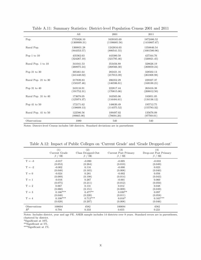
Table A.11: Summary Statistics: District-level Population Census 2001 and 2011

All 2001 2011

Pop. 1755826.10 1639165.69 1872486.52(1309999.31) (1190685.58) (1410807.67)

Rural Pop. 1300831.28 1242816.03 1358846.54(944353.57) (880541.55) (1001580.96)

Pop 1 to 10 435362.63 443380.50 427344.76(324267.10) (321795.46) (326821.45)

Rural Pop. 1 to 10 341041.53 353456.88 328626.19(268975.24) (268566.30) (269059.24)

Pop 21 to 30 305461.64 282421.16 328502.13(241448.02) (217013.39) (261808.98)

Rural Pop. 21 to 30 217839.83 206352.29 229327.37(158107.46) (146596.81) (168188.21)

Pop 31 to 40 243116.91 222817.44 263416.38(191752.31) (170815.06) (208812.50)

Rural Pop. 31 to 40 173678.05 163505.06 183851.05(125974.37) (116484.61) (134136.12)

Pop 41 to 50 172171.62 148630.49 195712.75(138609.13) (114375.52) (155783.32)

Rural Pop. 41 to 50 122586.56 109497.02 135676.09(89665.90) (78694.20) (97769.01)

Observations 1080 540 540

Notes: District-level Census includes 540 districts. Standard deviations are in parentheses

Table A.12: Impact of Public Colleges on ‘Current Grade’ and ‘Grade Dropped-out’

(1) (2) (3) (4)Current Grade Class Dropped-Out Current Post Primary Drop-out Post Primary

β / SE β / SE β / SE β / SE

T = -3 -0.017 -0.090 -0.005 -0.033(0.053) (0.264) (0.010) (0.049)

T = -2 -0.002 0.116 -0.000 0.023(0.048) (0.165) (0.008) (0.040)

T = 0 -0.024 0.281 -0.002 0.056(0.089) (0.198) (0.014) (0.043)

T = 1 -0.016 0.267 -0.001 0.060(0.075) (0.211) (0.012) (0.050)

T = 2 0.067 0.131 0.012 0.048(0.060) (0.151) (0.009) (0.049)

T = 3 0.166*** 0.477** 0.030** 0.097(0.048) (0.220) (0.011) (0.058)

T = 4 0.108*** 0.712*** 0.016* 0.165***(0.028) (0.207) (0.008) (0.046)

Observations 100694 4582 100694 4582R2 0.794 0.333 0.655 0.221

Notes: Includes district, year and age FE. ASER sample includes 14 districts over 9 years. Standard errors are in parentheses,clustered by district.*Significant at 10%.**Significant at 5%.***Significant at 1%.

x

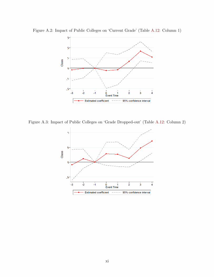
Figure A.2: Impact of Public Colleges on ‘Current Grade’ (Table A.12: Column 1)

Figure A.3: Impact of Public Colleges on ‘Grade Dropped-out’ (Table A.12: Column 2)

xi

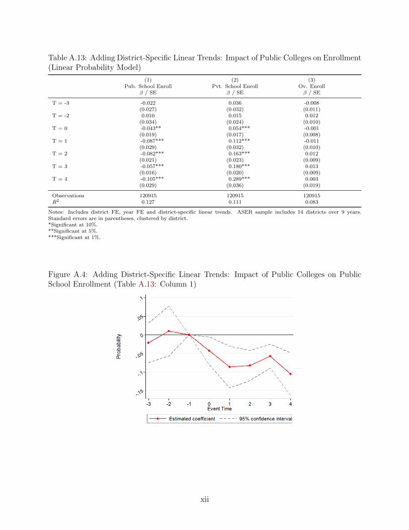
Table A.13: Adding District-Specific Linear Trends: Impact of Public Colleges on Enrollment(Linear Probability Model)

(1) (2) (3)Pub. School Enroll Pvt. School Enroll Ov. Enroll

β / SE β / SE β / SE

T = -3 -0.022 0.036 -0.008(0.027) (0.032) (0.011)

T = -2 0.010 0.015 0.012(0.034) (0.024) (0.010)

T = 0 -0.043** 0.054*** -0.001(0.019) (0.017) (0.008)

T = 1 -0.087*** 0.112*** -0.011(0.029) (0.032) (0.010)

T = 2 -0.082*** 0.163*** 0.012(0.021) (0.023) (0.009)

T = 3 -0.057*** 0.180*** 0.013(0.016) (0.020) (0.009)

T = 4 -0.105*** 0.289*** 0.003(0.029) (0.036) (0.019)

Observations 120915 120915 120915R2 0.127 0.111 0.083

Notes: Includes district FE, year FE and district-specific linear trends. ASER sample includes 14 districts over 9 years.Standard errors are in parentheses, clustered by district.*Significant at 10%.**Significant at 5%.***Significant at 1%.

Figure A.4: Adding District-Specific Linear Trends: Impact of Public Colleges on PublicSchool Enrollment (Table A.13: Column 1)

xii

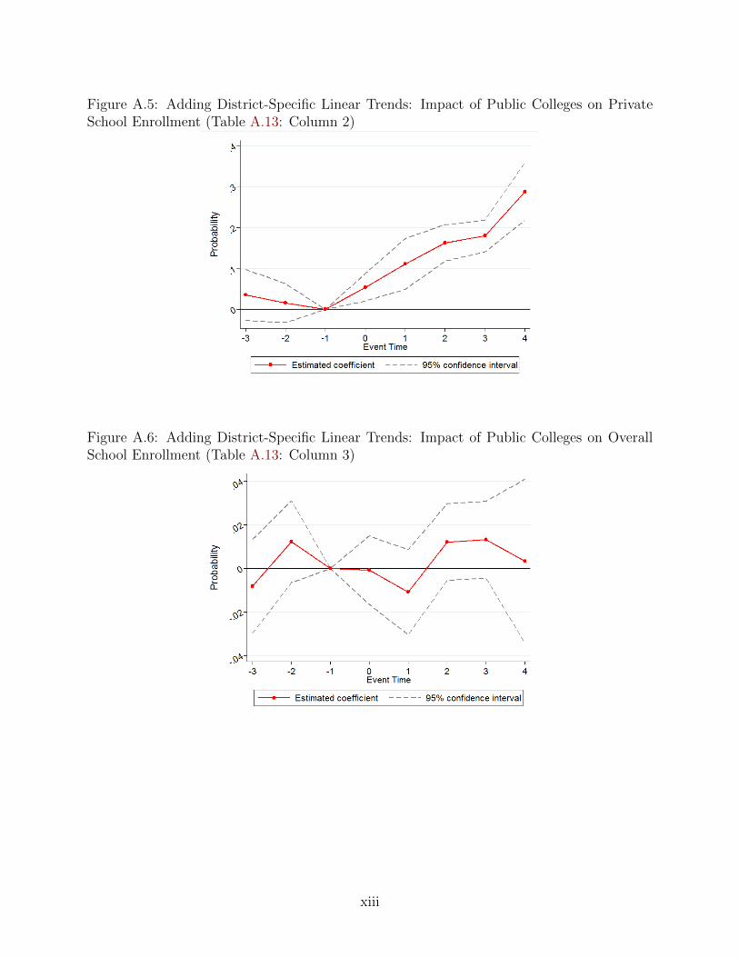
Figure A.5: Adding District-Specific Linear Trends: Impact of Public Colleges on PrivateSchool Enrollment (Table A.13: Column 2)

Figure A.6: Adding District-Specific Linear Trends: Impact of Public Colleges on OverallSchool Enrollment (Table A.13: Column 3)

xiii

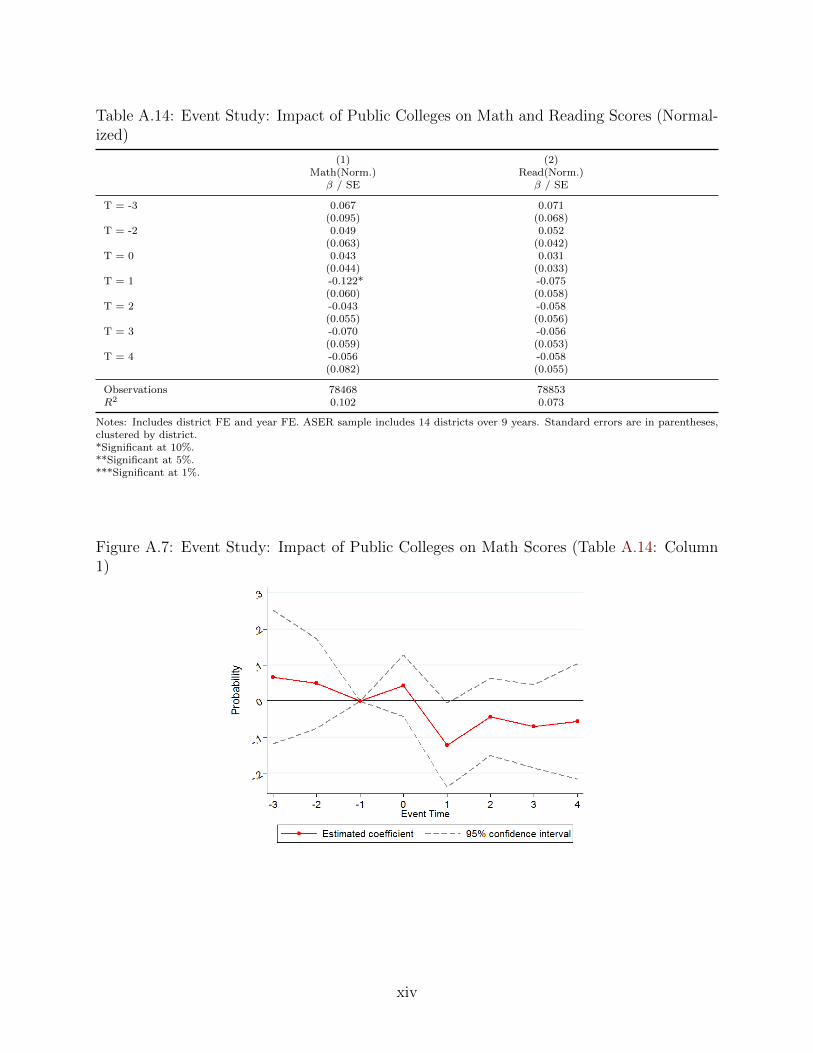
Table A.14: Event Study: Impact of Public Colleges on Math and Reading Scores (Normal-ized)

(1) (2)Math(Norm.) Read(Norm.)

β / SE β / SE

T = -3 0.067 0.071(0.095) (0.068)

T = -2 0.049 0.052(0.063) (0.042)

T = 0 0.043 0.031(0.044) (0.033)

T = 1 -0.122* -0.075(0.060) (0.058)

T = 2 -0.043 -0.058(0.055) (0.056)

T = 3 -0.070 -0.056(0.059) (0.053)

T = 4 -0.056 -0.058(0.082) (0.055)

Observations 78468 78853R2 0.102 0.073

Notes: Includes district FE and year FE. ASER sample includes 14 districts over 9 years. Standard errors are in parentheses,clustered by district.*Significant at 10%.**Significant at 5%.***Significant at 1%.

Figure A.7: Event Study: Impact of Public Colleges on Math Scores (Table A.14: Column1)

xiv

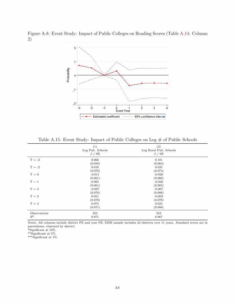
Figure A.8: Event Study: Impact of Public Colleges on Reading Scores (Table A.14: Column2)

Table A.15: Event Study: Impact of Public Colleges on Log # of Public Schools

(1) (2)Log Pub. Schools Log Rural Pub. Schools

β / SE β / SE

T = -3 0.066 0.101(0.058) (0.064)

T = -2 0.010 0.025(0.070) (0.074)

T = 0 -0.011 -0.026(0.061) (0.066)

T = 1 0.005 -0.020(0.061) (0.065)

T = 2 -0.007 -0.067(0.076) (0.086)

T = 3 0.051 -0.003(0.070) (0.079)

T = 4 0.074 0.024(0.071) (0.088)

Observations 253 253R2 0.971 0.967

Notes: All columns include district FE and year FE. DISE sample includes 23 districts over 11 years. Standard errors are inparentheses, clustered by district.*Significant at 10%.**Significant at 5%.***Significant at 1%.

xv

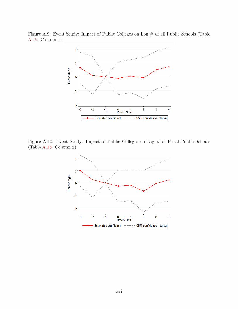
Figure A.9: Event Study: Impact of Public Colleges on Log # of all Public Schools (TableA.15: Column 1)

Figure A.10: Event Study: Impact of Public Colleges on Log # of Rural Public Schools(Table A.15: Column 2)

xvi

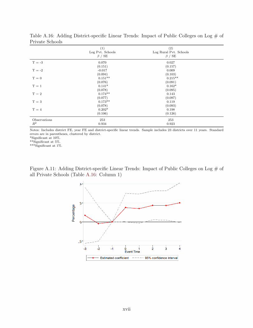
Table A.16: Adding District-specific Linear Trends: Impact of Public Colleges on Log # ofPrivate Schools

(1) (2)Log Pvt. Schools Log Rural Pvt. Schools

β / SE β / SE

T = -3 0.070 0.027(0.151) (0.157)

T = -2 -0.017 0.009(0.094) (0.103)

T = 0 0.151** 0.215**(0.076) (0.091)

T = 1 0.141* 0.162*(0.078) (0.095)

T = 2 0.174** 0.143(0.077) (0.097)

T = 3 0.173** 0.119(0.078) (0.093)

T = 4 0.202* 0.198(0.106) (0.126)

Observations 253 253R2 0.934 0.923

Notes: Includes district FE, year FE and district-specific linear trends. Sample includes 23 districts over 11 years. Standarderrors are in parentheses, clustered by district.*Significant at 10%.**Significant at 5%.***Significant at 1%.

Figure A.11: Adding District-specific Linear Trends: Impact of Public Colleges on Log # ofall Private Schools (Table A.16: Column 1)

xvii

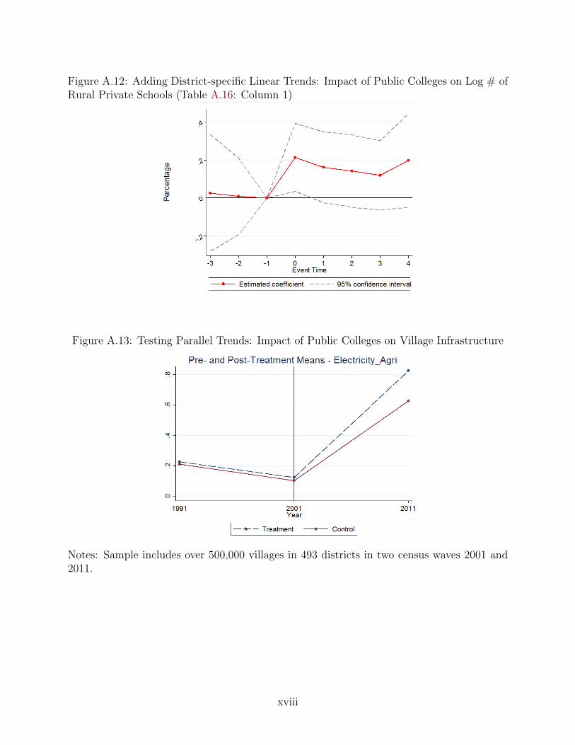
Figure A.12: Adding District-specific Linear Trends: Impact of Public Colleges on Log # ofRural Private Schools (Table A.16: Column 1)

Figure A.13: Testing Parallel Trends: Impact of Public Colleges on Village Infrastructure

Notes: Sample includes over 500,000 villages in 493 districts in two census waves 2001 and2011.

xviii

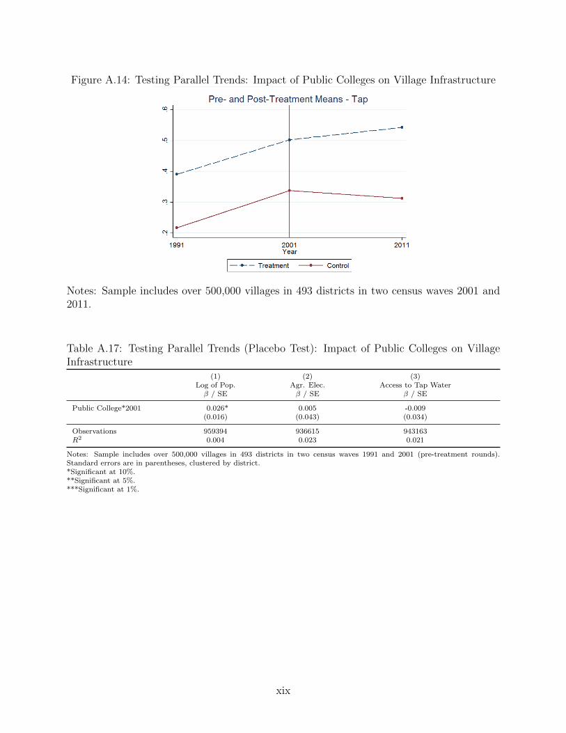
Figure A.14: Testing Parallel Trends: Impact of Public Colleges on Village Infrastructure

Notes: Sample includes over 500,000 villages in 493 districts in two census waves 2001 and2011.

Table A.17: Testing Parallel Trends (Placebo Test): Impact of Public Colleges on VillageInfrastructure

(1) (2) (3)Log of Pop. Agr. Elec. Access to Tap Waterβ / SE β / SE β / SE

Public College*2001 0.026* 0.005 -0.009(0.016) (0.043) (0.034)

Observations 959394 936615 943163R2 0.004 0.023 0.021

Notes: Sample includes over 500,000 villages in 493 districts in two census waves 1991 and 2001 (pre-treatment rounds).Standard errors are in parentheses, clustered by district.*Significant at 10%.**Significant at 5%.***Significant at 1%.

xix

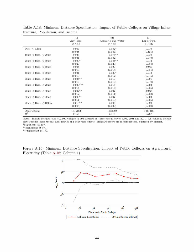
Table A.18: Minimum Distance Specification: Impact of Public Colleges on Village Infras-tructure, Population, and Income

(1) (2) (3)Agr. Elec. Access to Tap Water Log of Pop.β / SE β / SE β / SE

Dist. < 10km 0.007 0.082* 0.010(0.048) (0.047) (0.121)

10km < Dist. < 20km 0.043 0.076** 0.030(0.031) (0.032) (0.079)

20km < Dist. < 30km 0.039* 0.044** 0.012(0.020) (0.020) (0.058)

30km < Dist. < 40km 0.028 0.029 -0.009(0.019) (0.018) (0.051)

40km < Dist. < 50km 0.031 0.030* 0.013(0.019) (0.017) (0.045)

50km < Dist. < 60km 0.038** 0.019 0.001(0.016) (0.015) (0.040)

60km < Dist. < 70km 0.039*** 0.016 0.003(0.014) (0.013) (0.036)

70km < Dist. < 80km 0.027** 0.007 -0.025(0.012) (0.011) (0.032)

80km < Dist. < 90km 0.020* 0.007 0.003(0.011) (0.010) (0.025)

90km < Dist. < 100km 0.018** 0.005 0.022(0.008) (0.009) (0.020)

Observations 1315183 1358089 1441416R2 0.456 0.413 0.287

Notes: Sample includes over 500,000 villages in 493 districts in three census waves 1991, 2001 and 2011. All columns includestate-specific linear trends, and district and year fixed effects. Standard errors are in parentheses, clustered by district.*Significant at 10%.**Significant at 5%.***Significant at 1%.

Figure A.15: Minimum Distance Specification: Impact of Public Colleges on AgriculturalElectricity (Table A.18: Column 1)

xx

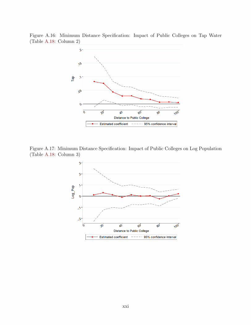
Figure A.16: Minimum Distance Specification: Impact of Public Colleges on Tap Water(Table A.18: Column 2)

Figure A.17: Minimum Distance Specification: Impact of Public Colleges on Log Population(Table A.18: Column 3)

xxi

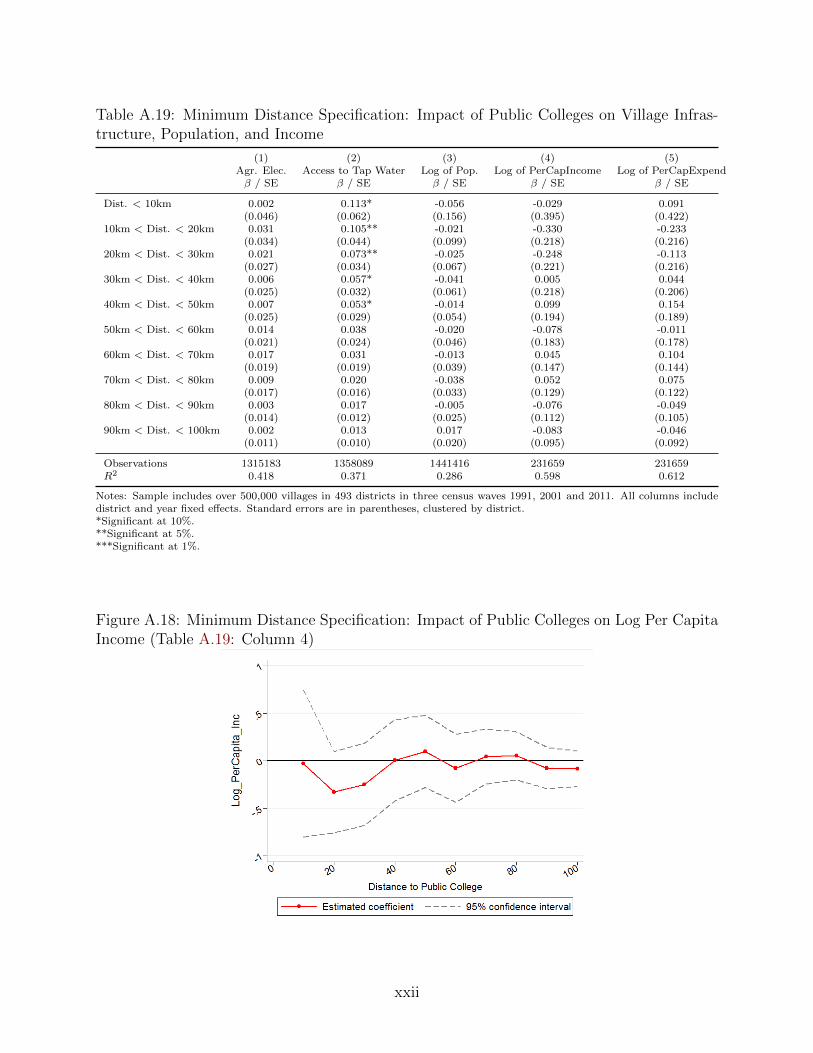
Table A.19: Minimum Distance Specification: Impact of Public Colleges on Village Infras-tructure, Population, and Income

(1) (2) (3) (4) (5)Agr. Elec. Access to Tap Water Log of Pop. Log of PerCapIncome Log of PerCapExpendβ / SE β / SE β / SE β / SE β / SE

Dist. < 10km 0.002 0.113* -0.056 -0.029 0.091(0.046) (0.062) (0.156) (0.395) (0.422)

10km < Dist. < 20km 0.031 0.105** -0.021 -0.330 -0.233(0.034) (0.044) (0.099) (0.218) (0.216)

20km < Dist. < 30km 0.021 0.073** -0.025 -0.248 -0.113(0.027) (0.034) (0.067) (0.221) (0.216)

30km < Dist. < 40km 0.006 0.057* -0.041 0.005 0.044(0.025) (0.032) (0.061) (0.218) (0.206)

40km < Dist. < 50km 0.007 0.053* -0.014 0.099 0.154(0.025) (0.029) (0.054) (0.194) (0.189)

50km < Dist. < 60km 0.014 0.038 -0.020 -0.078 -0.011(0.021) (0.024) (0.046) (0.183) (0.178)

60km < Dist. < 70km 0.017 0.031 -0.013 0.045 0.104(0.019) (0.019) (0.039) (0.147) (0.144)

70km < Dist. < 80km 0.009 0.020 -0.038 0.052 0.075(0.017) (0.016) (0.033) (0.129) (0.122)

80km < Dist. < 90km 0.003 0.017 -0.005 -0.076 -0.049(0.014) (0.012) (0.025) (0.112) (0.105)

90km < Dist. < 100km 0.002 0.013 0.017 -0.083 -0.046(0.011) (0.010) (0.020) (0.095) (0.092)

Observations 1315183 1358089 1441416 231659 231659R2 0.418 0.371 0.286 0.598 0.612

Notes: Sample includes over 500,000 villages in 493 districts in three census waves 1991, 2001 and 2011. All columns includedistrict and year fixed effects. Standard errors are in parentheses, clustered by district.*Significant at 10%.**Significant at 5%.***Significant at 1%.

Figure A.18: Minimum Distance Specification: Impact of Public Colleges on Log Per CapitaIncome (Table A.19: Column 4)

xxii

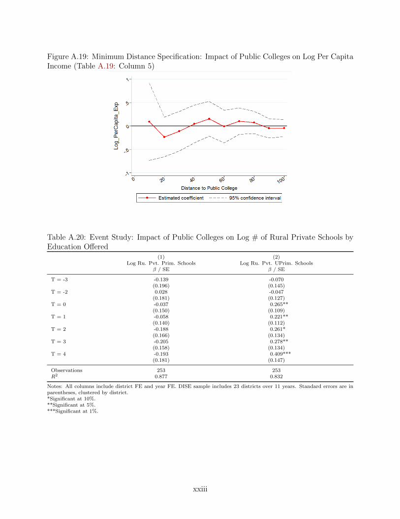
Figure A.19: Minimum Distance Specification: Impact of Public Colleges on Log Per CapitaIncome (Table A.19: Column 5)

Table A.20: Event Study: Impact of Public Colleges on Log # of Rural Private Schools byEducation Offered

(1) (2)Log Ru. Pvt. Prim. Schools Log Ru. Pvt. UPrim. Schools

β / SE β / SE

T = -3 -0.139 -0.070(0.196) (0.145)

T = -2 0.028 -0.047(0.181) (0.127)

T = 0 -0.037 0.265**(0.150) (0.109)

T = 1 -0.058 0.221**(0.140) (0.112)

T = 2 -0.188 0.261*(0.166) (0.134)

T = 3 -0.205 0.278**(0.158) (0.134)

T = 4 -0.193 0.409***(0.181) (0.147)

Observations 253 253R2 0.877 0.832

Notes: All columns include district FE and year FE. DISE sample includes 23 districts over 11 years. Standard errors are inparentheses, clustered by district.*Significant at 10%.**Significant at 5%.***Significant at 1%.

xxiii

Figure A.20: Event Study: Impact of Public Colleges on Log # of Rural Private SchoolsOffering Only Primary Education (Table A.20: Column 1)

Figure A.21: Event Study: Impact of Public Colleges on Log # of Rural Private SchoolsOffering Upper-Primary Education and Above (Table A.20: Column 2)

xxiv

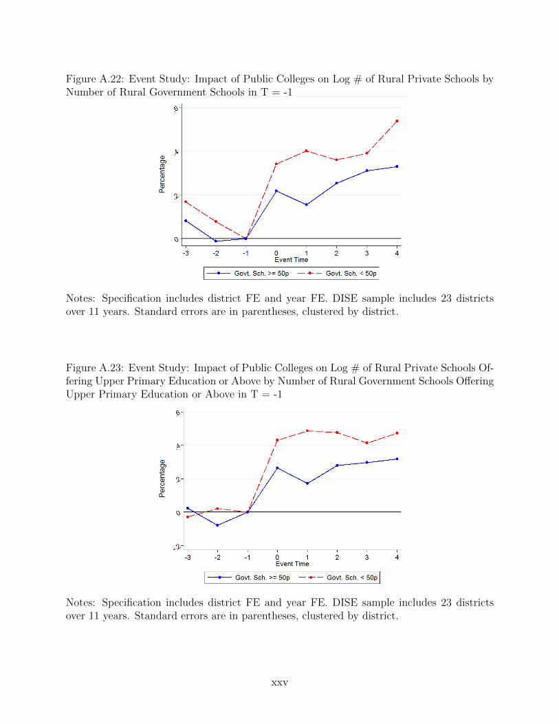
Figure A.22: Event Study: Impact of Public Colleges on Log # of Rural Private Schools byNumber of Rural Government Schools in T = -1

Notes: Specification includes district FE and year FE. DISE sample includes 23 districtsover 11 years. Standard errors are in parentheses, clustered by district.

Figure A.23: Event Study: Impact of Public Colleges on Log # of Rural Private Schools Of-fering Upper Primary Education or Above by Number of Rural Government Schools OfferingUpper Primary Education or Above in T = -1

Notes: Specification includes district FE and year FE. DISE sample includes 23 districtsover 11 years. Standard errors are in parentheses, clustered by district.

xxv

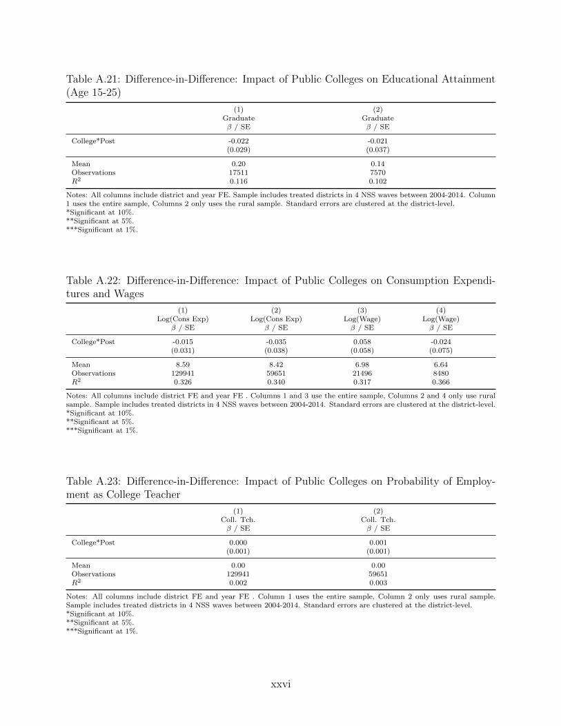
Table A.21: Difference-in-Difference: Impact of Public Colleges on Educational Attainment(Age 15-25)

(1) (2)Graduate Graduateβ / SE β / SE

College*Post -0.022 -0.021(0.029) (0.037)

Mean 0.20 0.14Observations 17511 7570R2 0.116 0.102

Notes: All columns include district and year FE. Sample includes treated districts in 4 NSS waves between 2004-2014. Column1 uses the entire sample, Columns 2 only uses the rural sample. Standard errors are clustered at the district-level.*Significant at 10%.**Significant at 5%.***Significant at 1%.

Table A.22: Difference-in-Difference: Impact of Public Colleges on Consumption Expendi-tures and Wages

(1) (2) (3) (4)Log(Cons Exp) Log(Cons Exp) Log(Wage) Log(Wage)

β / SE β / SE β / SE β / SE

College*Post -0.015 -0.035 0.058 -0.024(0.031) (0.038) (0.058) (0.075)

Mean 8.59 8.42 6.98 6.64Observations 129941 59651 21496 8480R2 0.326 0.340 0.317 0.366

Notes: All columns include district FE and year FE . Columns 1 and 3 use the entire sample, Columns 2 and 4 only use ruralsample. Sample includes treated districts in 4 NSS waves between 2004-2014. Standard errors are clustered at the district-level.*Significant at 10%.**Significant at 5%.***Significant at 1%.

Table A.23: Difference-in-Difference: Impact of Public Colleges on Probability of Employ-ment as College Teacher

(1) (2)Coll. Tch. Coll. Tch.β / SE β / SE

College*Post 0.000 0.001(0.001) (0.001)

Mean 0.00 0.00Observations 129941 59651R2 0.002 0.003

Notes: All columns include district FE and year FE . Column 1 uses the entire sample, Column 2 only uses rural sample.Sample includes treated districts in 4 NSS waves between 2004-2014. Standard errors are clustered at the district-level.*Significant at 10%.**Significant at 5%.***Significant at 1%.

xxvi

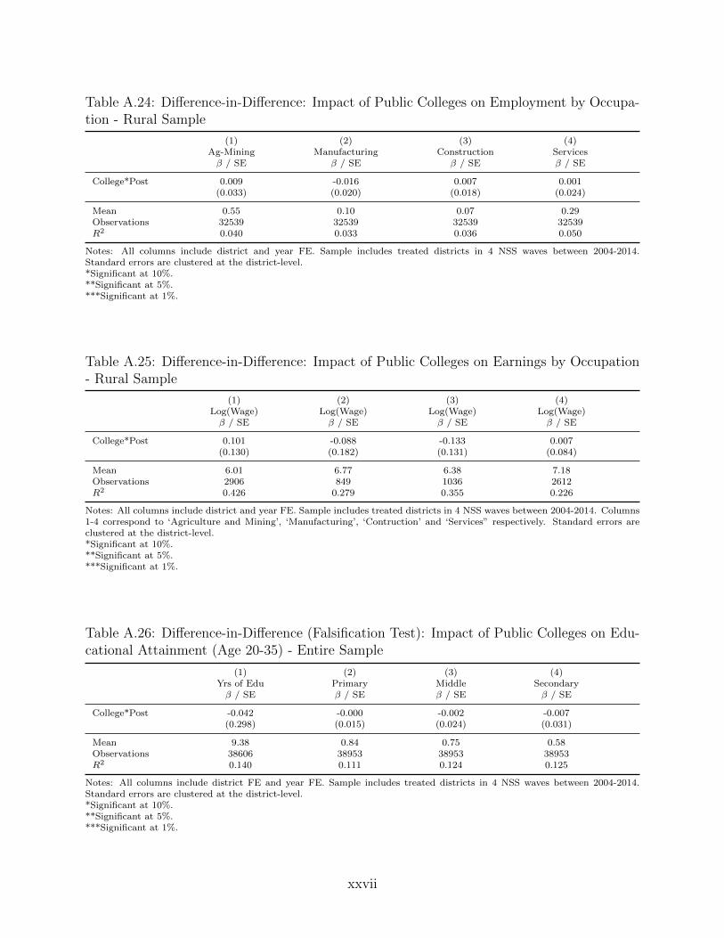
Table A.24: Difference-in-Difference: Impact of Public Colleges on Employment by Occupa-tion - Rural Sample

(1) (2) (3) (4)Ag-Mining Manufacturing Construction Servicesβ / SE β / SE β / SE β / SE

College*Post 0.009 -0.016 0.007 0.001(0.033) (0.020) (0.018) (0.024)

Mean 0.55 0.10 0.07 0.29Observations 32539 32539 32539 32539R2 0.040 0.033 0.036 0.050

Notes: All columns include district and year FE. Sample includes treated districts in 4 NSS waves between 2004-2014.Standard errors are clustered at the district-level.*Significant at 10%.**Significant at 5%.***Significant at 1%.

Table A.25: Difference-in-Difference: Impact of Public Colleges on Earnings by Occupation- Rural Sample

(1) (2) (3) (4)Log(Wage) Log(Wage) Log(Wage) Log(Wage)β / SE β / SE β / SE β / SE

College*Post 0.101 -0.088 -0.133 0.007(0.130) (0.182) (0.131) (0.084)

Mean 6.01 6.77 6.38 7.18Observations 2906 849 1036 2612R2 0.426 0.279 0.355 0.226

Notes: All columns include district and year FE. Sample includes treated districts in 4 NSS waves between 2004-2014. Columns1-4 correspond to ‘Agriculture and Mining’, ‘Manufacturing’, ‘Contruction’ and ‘Services” respectively. Standard errors areclustered at the district-level.*Significant at 10%.**Significant at 5%.***Significant at 1%.

Table A.26: Difference-in-Difference (Falsification Test): Impact of Public Colleges on Edu-cational Attainment (Age 20-35) - Entire Sample

(1) (2) (3) (4)Yrs of Edu Primary Middle Secondaryβ / SE β / SE β / SE β / SE

College*Post -0.042 -0.000 -0.002 -0.007(0.298) (0.015) (0.024) (0.031)

Mean 9.38 0.84 0.75 0.58Observations 38606 38953 38953 38953R2 0.140 0.111 0.124 0.125

Notes: All columns include district FE and year FE. Sample includes treated districts in 4 NSS waves between 2004-2014.Standard errors are clustered at the district-level.*Significant at 10%.**Significant at 5%.***Significant at 1%.

xxvii

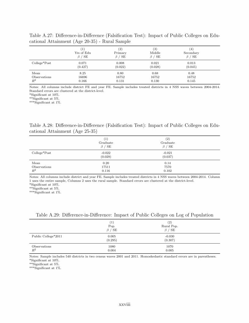
Table A.27: Difference-in-Difference (Falsification Test): Impact of Public Colleges on Edu-cational Attainment (Age 20-35) - Rural Sample

(1) (2) (3) (4)Yrs of Edu Primary Middle Secondaryβ / SE β / SE β / SE β / SE

College*Post 0.071 0.008 0.021 0.013(0.427) (0.022) (0.028) (0.045)

Mean 8.25 0.80 0.68 0.48Observations 16696 16752 16752 16752R2 0.166 0.131 0.130 0.145

Notes: All columns include district FE and year FE. Sample includes treated districts in 4 NSS waves between 2004-2014.Standard errors are clustered at the district-level.*Significant at 10%.**Significant at 5%.***Significant at 1%.

Table A.28: Difference-in-Difference (Falsification Test): Impact of Public Colleges on Edu-cational Attainment (Age 25-35)

(1) (2)Graduate Graduateβ / SE β / SE

College*Post -0.022 -0.021(0.029) (0.037)

Mean 0.20 0.14Observations 17511 7570R2 0.116 0.102

Notes: All columns include district and year FE. Sample includes treated districts in 4 NSS waves between 2004-2014. Column1 uses the entire sample, Columns 2 uses the rural sample. Standard errors are clustered at the district-level.*Significant at 10%.**Significant at 5%.***Significant at 1%.

Table A.29: Difference-in-Difference: Impact of Public Colleges on Log of Population

(1) (2)Pop. Rural Pop.β / SE β / SE

Public College*2011 0.005 -0.030(0.295) (0.307)

Observations 1080 1070R2 0.004 0.005

Notes: Sample includes 540 districts in two census waves 2001 and 2011. Homoskedastic standard errors are in parentheses.*Significant at 10%.**Significant at 5%.***Significant at 1%.

xxviii

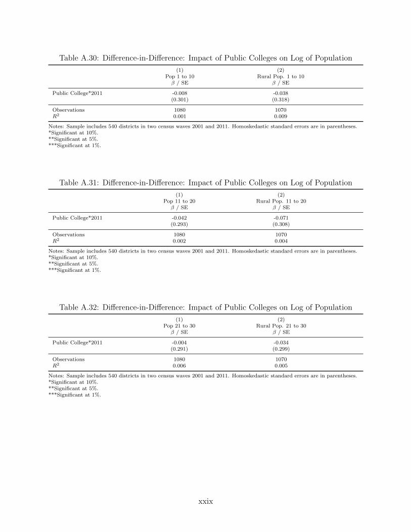
Table A.30: Difference-in-Difference: Impact of Public Colleges on Log of Population

(1) (2)Pop 1 to 10 Rural Pop. 1 to 10β / SE β / SE

Public College*2011 -0.008 -0.038(0.301) (0.318)

Observations 1080 1070R2 0.001 0.009

Notes: Sample includes 540 districts in two census waves 2001 and 2011. Homoskedastic standard errors are in parentheses.*Significant at 10%.**Significant at 5%.***Significant at 1%.

Table A.31: Difference-in-Difference: Impact of Public Colleges on Log of Population

(1) (2)Pop 11 to 20 Rural Pop. 11 to 20β / SE β / SE

Public College*2011 -0.042 -0.071(0.293) (0.308)

Observations 1080 1070R2 0.002 0.004

Notes: Sample includes 540 districts in two census waves 2001 and 2011. Homoskedastic standard errors are in parentheses.*Significant at 10%.**Significant at 5%.***Significant at 1%.

Table A.32: Difference-in-Difference: Impact of Public Colleges on Log of Population

(1) (2)Pop 21 to 30 Rural Pop. 21 to 30β / SE β / SE

Public College*2011 -0.004 -0.034(0.291) (0.299)

Observations 1080 1070R2 0.006 0.005

Notes: Sample includes 540 districts in two census waves 2001 and 2011. Homoskedastic standard errors are in parentheses.*Significant at 10%.**Significant at 5%.***Significant at 1%.

xxix

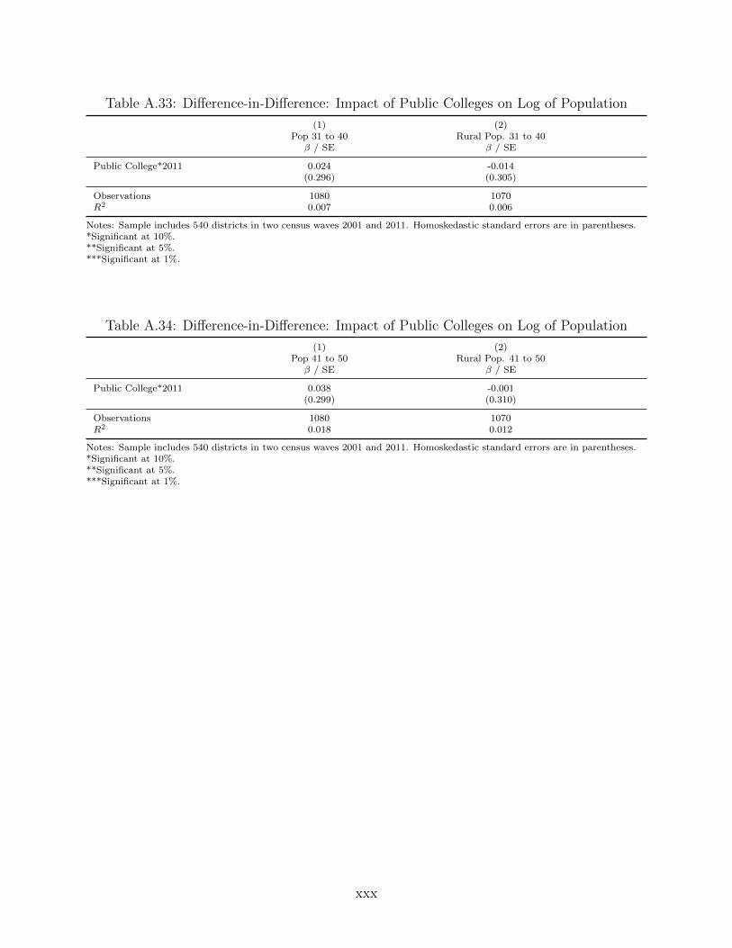
Table A.33: Difference-in-Difference: Impact of Public Colleges on Log of Population

(1) (2)Pop 31 to 40 Rural Pop. 31 to 40β / SE β / SE

Public College*2011 0.024 -0.014(0.296) (0.305)

Observations 1080 1070R2 0.007 0.006

Notes: Sample includes 540 districts in two census waves 2001 and 2011. Homoskedastic standard errors are in parentheses.*Significant at 10%.**Significant at 5%.***Significant at 1%.

Table A.34: Difference-in-Difference: Impact of Public Colleges on Log of Population

(1) (2)Pop 41 to 50 Rural Pop. 41 to 50β / SE β / SE

Public College*2011 0.038 -0.001(0.299) (0.310)

Observations 1080 1070R2 0.018 0.012

Notes: Sample includes 540 districts in two census waves 2001 and 2011. Homoskedastic standard errors are in parentheses.*Significant at 10%.**Significant at 5%.***Significant at 1%.

xxx

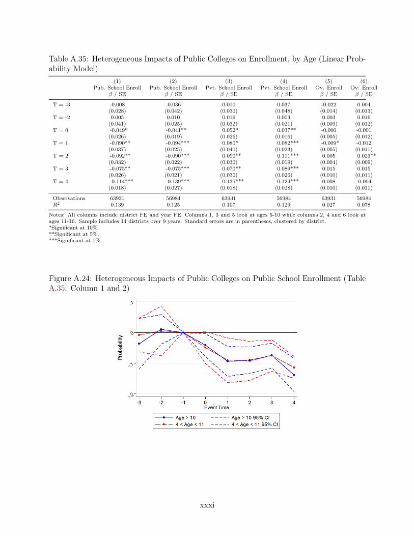
Table A.35: Heterogeneous Impacts of Public Colleges on Enrollment, by Age (Linear Prob-ability Model)

(1) (2) (3) (4) (5) (6)Pub. School Enroll Pub. School Enroll Pvt. School Enroll Pvt. School Enroll Ov. Enroll Ov. Enroll

β / SE β / SE β / SE β / SE β / SE β / SE

T = -3 -0.008 -0.036 0.010 0.037 -0.022 0.004(0.028) (0.042) (0.030) (0.048) (0.014) (0.013)

T = -2 0.005 0.010 0.016 0.004 0.003 0.016(0.041) (0.025) (0.032) (0.021) (0.009) (0.012)

T = 0 -0.049* -0.041** 0.052* 0.037** -0.000 -0.001(0.026) (0.019) (0.026) (0.016) (0.005) (0.012)

T = 1 -0.090** -0.094*** 0.080* 0.082*** -0.009* -0.012(0.037) (0.025) (0.040) (0.023) (0.005) (0.011)

T = 2 -0.092** -0.090*** 0.090** 0.111*** 0.005 0.023**(0.032) (0.022) (0.030) (0.019) (0.004) (0.009)

T = 3 -0.075** -0.075*** 0.070** 0.089*** 0.015 0.015(0.026) (0.021) (0.030) (0.026) (0.010) (0.011)

T = 4 -0.114*** -0.139*** 0.135*** 0.124*** 0.008 -0.004(0.018) (0.027) (0.018) (0.028) (0.010) (0.011)

Observations 63931 56984 63931 56984 63931 56984R2 0.139 0.125 0.107 0.129 0.027 0.078

Notes: All columns include district FE and year FE. Columns 1, 3 and 5 look at ages 5-10 while columns 2, 4 and 6 look atages 11-16. Sample includes 14 districts over 9 years. Standard errors are in parentheses, clustered by district.*Significant at 10%.**Significant at 5%.***Significant at 1%.

Figure A.24: Heterogeneous Impacts of Public Colleges on Public School Enrollment (TableA.35: Column 1 and 2)

xxxi

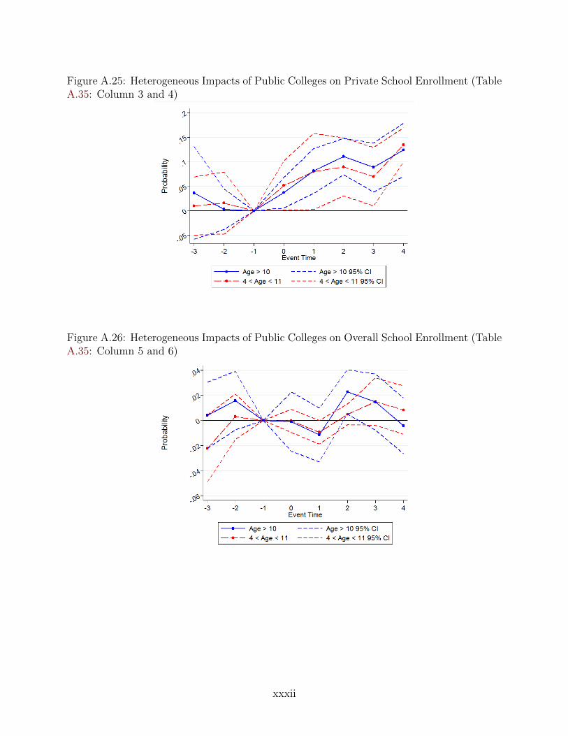
Figure A.25: Heterogeneous Impacts of Public Colleges on Private School Enrollment (TableA.35: Column 3 and 4)

Figure A.26: Heterogeneous Impacts of Public Colleges on Overall School Enrollment (TableA.35: Column 5 and 6)

xxxii

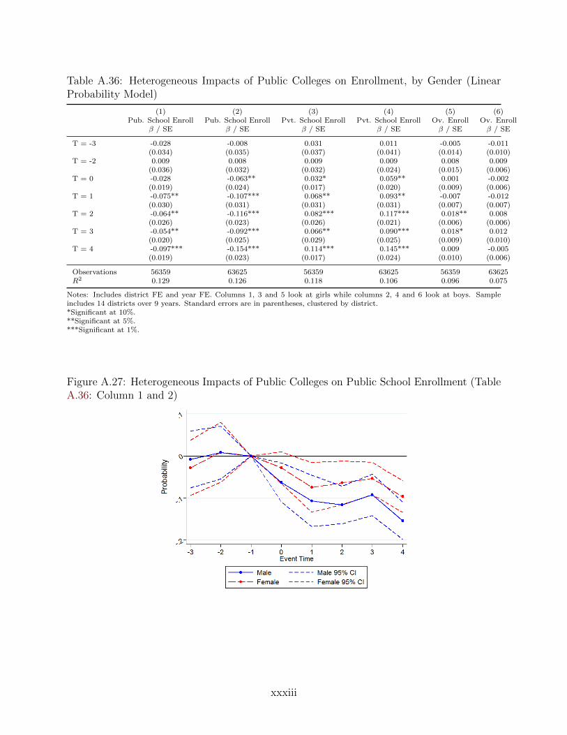
Table A.36: Heterogeneous Impacts of Public Colleges on Enrollment, by Gender (LinearProbability Model)

(1) (2) (3) (4) (5) (6)Pub. School Enroll Pub. School Enroll Pvt. School Enroll Pvt. School Enroll Ov. Enroll Ov. Enroll

β / SE β / SE β / SE β / SE β / SE β / SE

T = -3 -0.028 -0.008 0.031 0.011 -0.005 -0.011(0.034) (0.035) (0.037) (0.041) (0.014) (0.010)

T = -2 0.009 0.008 0.009 0.009 0.008 0.009(0.036) (0.032) (0.032) (0.024) (0.015) (0.006)

T = 0 -0.028 -0.063** 0.032* 0.059** 0.001 -0.002(0.019) (0.024) (0.017) (0.020) (0.009) (0.006)

T = 1 -0.075** -0.107*** 0.068** 0.093** -0.007 -0.012(0.030) (0.031) (0.031) (0.031) (0.007) (0.007)

T = 2 -0.064** -0.116*** 0.082*** 0.117*** 0.018** 0.008(0.026) (0.023) (0.026) (0.021) (0.006) (0.006)

T = 3 -0.054** -0.092*** 0.066** 0.090*** 0.018* 0.012(0.020) (0.025) (0.029) (0.025) (0.009) (0.010)

T = 4 -0.097*** -0.154*** 0.114*** 0.145*** 0.009 -0.005(0.019) (0.023) (0.017) (0.024) (0.010) (0.006)

Observations 56359 63625 56359 63625 56359 63625R2 0.129 0.126 0.118 0.106 0.096 0.075

Notes: Includes district FE and year FE. Columns 1, 3 and 5 look at girls while columns 2, 4 and 6 look at boys. Sampleincludes 14 districts over 9 years. Standard errors are in parentheses, clustered by district.*Significant at 10%.**Significant at 5%.***Significant at 1%.

Figure A.27: Heterogeneous Impacts of Public Colleges on Public School Enrollment (TableA.36: Column 1 and 2)

xxxiii

Figure A.28: Heterogeneous Impacts of Public Colleges on Private School Enrollment (TableA.36: Column 3 and 4)

Figure A.29: Heterogeneous Impacts of Public Colleges on Overall School Enrollment (TableA.36: Column 5 and 6)

xxxiv

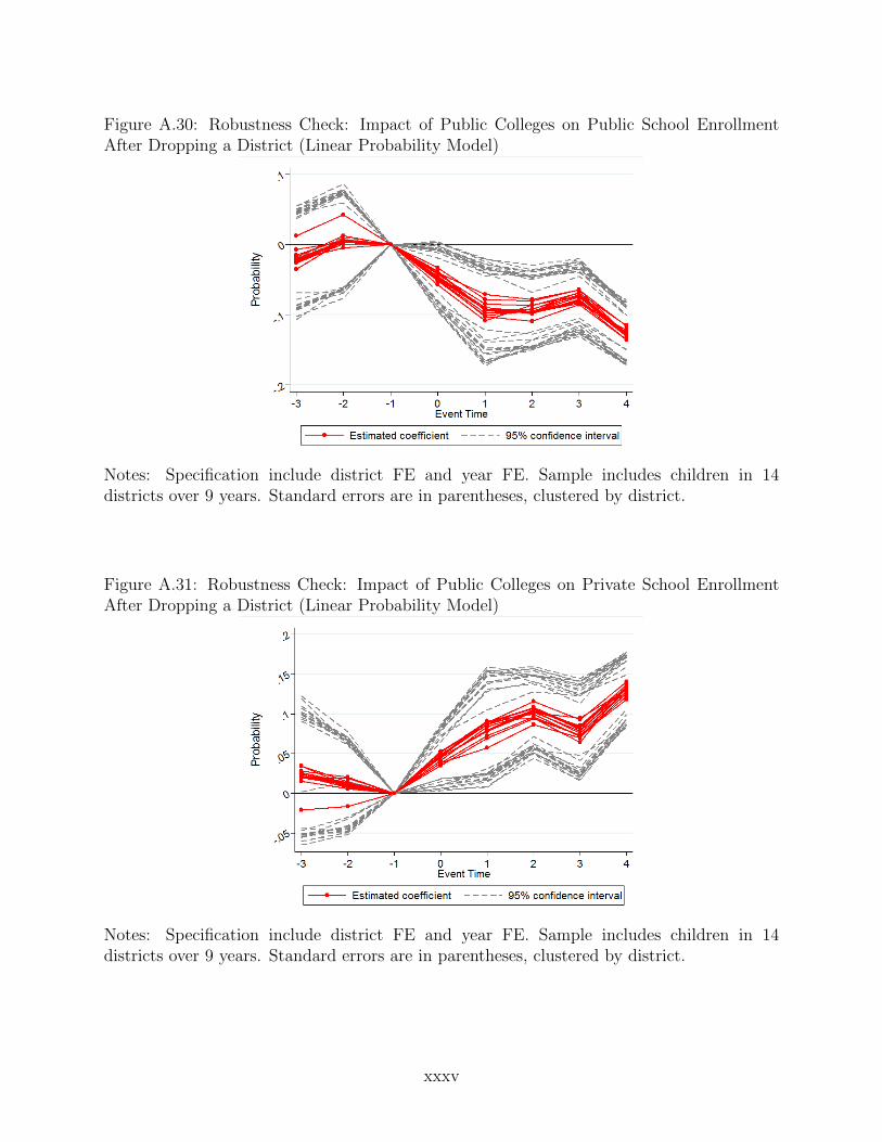
Figure A.30: Robustness Check: Impact of Public Colleges on Public School EnrollmentAfter Dropping a District (Linear Probability Model)

Notes: Specification include district FE and year FE. Sample includes children in 14districts over 9 years. Standard errors are in parentheses, clustered by district.

Figure A.31: Robustness Check: Impact of Public Colleges on Private School EnrollmentAfter Dropping a District (Linear Probability Model)

Notes: Specification include district FE and year FE. Sample includes children in 14districts over 9 years. Standard errors are in parentheses, clustered by district.

xxxv

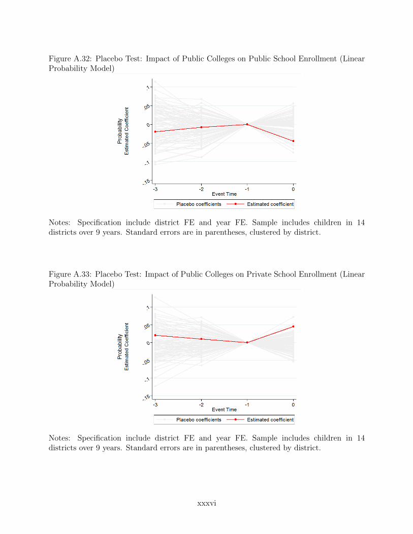
Figure A.32: Placebo Test: Impact of Public Colleges on Public School Enrollment (LinearProbability Model)

Notes: Specification include district FE and year FE. Sample includes children in 14districts over 9 years. Standard errors are in parentheses, clustered by district.

Figure A.33: Placebo Test: Impact of Public Colleges on Private School Enrollment (LinearProbability Model)

Notes: Specification include district FE and year FE. Sample includes children in 14districts over 9 years. Standard errors are in parentheses, clustered by district.

xxxvi

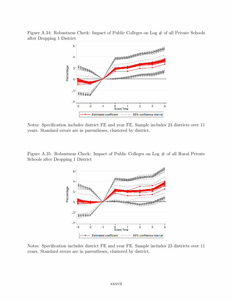
Figure A.34: Robustness Check: Impact of Public Colleges on Log # of all Private Schoolsafter Dropping 1 District

Notes: Specification includes district FE and year FE. Sample includes 23 districts over 11years. Standard errors are in parentheses, clustered by district.

Figure A.35: Robustness Check: Impact of Public Colleges on Log # of all Rural PrivateSchools after Dropping 1 District

Notes: Specification includes district FE and year FE. Sample includes 23 districts over 11years. Standard errors are in parentheses, clustered by district.

xxxvii

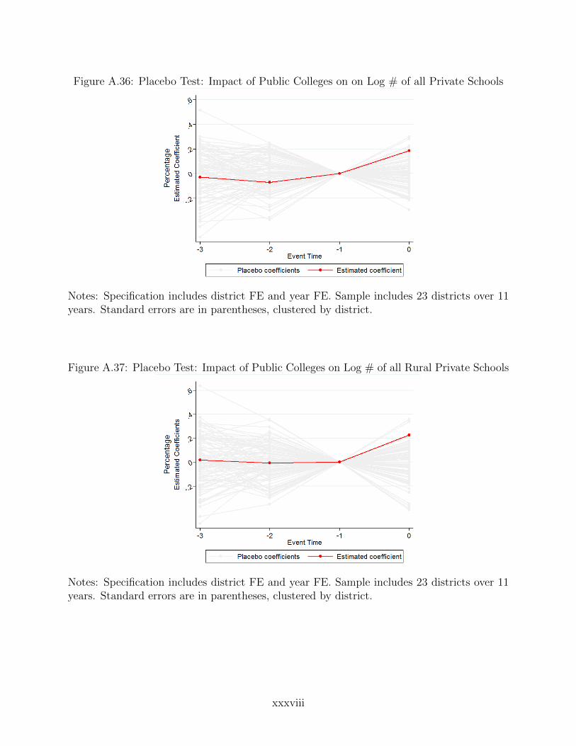
Figure A.36: Placebo Test: Impact of Public Colleges on on Log # of all Private Schools

Notes: Specification includes district FE and year FE. Sample includes 23 districts over 11years. Standard errors are in parentheses, clustered by district.

Figure A.37: Placebo Test: Impact of Public Colleges on Log # of all Rural Private Schools

Notes: Specification includes district FE and year FE. Sample includes 23 districts over 11years. Standard errors are in parentheses, clustered by district.

xxxviii