Triangulation Trigonometric Parallax

1

Chapter 13

Measuring the Properties of Stars

2

The Family of Stars

• Those tiny glints of light in the night sky are in reality huge, dazzling balls of gas, many of which are vastly larger and brighter than the Sun

• They look dim because of their vast distances• Astronomers cannot probe stars directly, and

consequently must devise indirect methods to ascertain their intrinsic properties

• Measuring distances to stars and galaxies is not easy

• Distance is very important for determining the intrinsic properties of astronomical objects

3

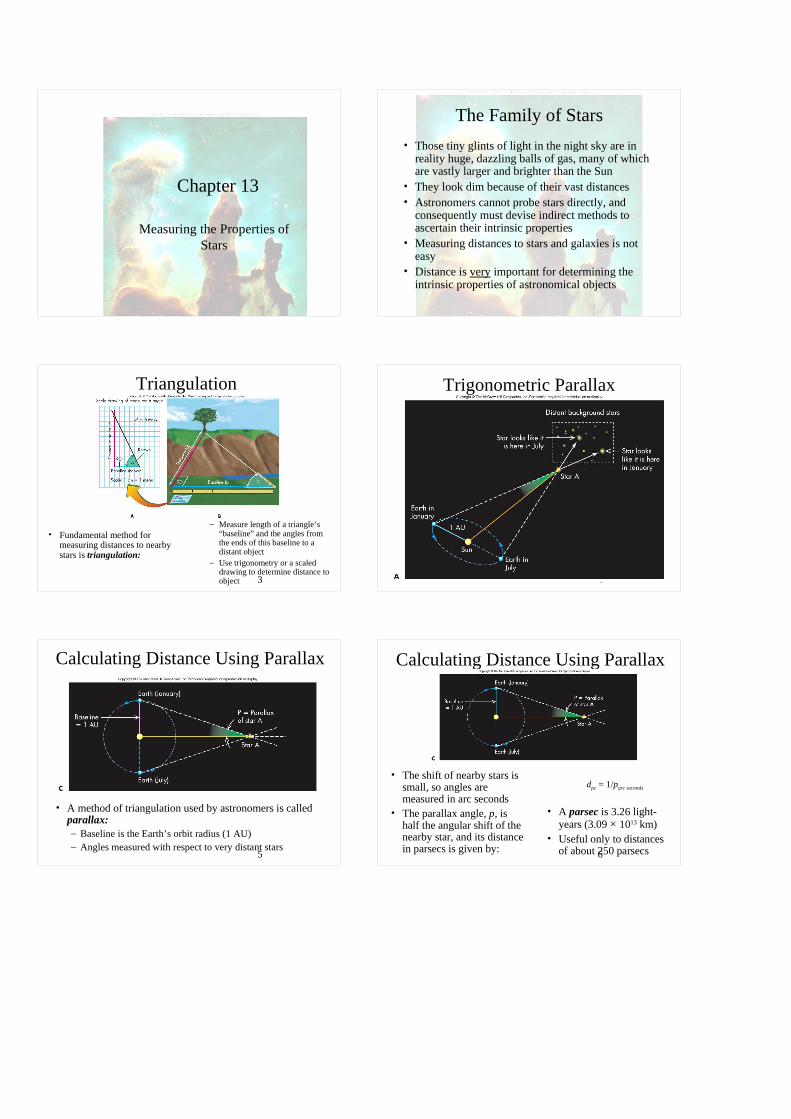
Triangulation

• Fundamental method for measuring distances to nearby stars is triangulation:

– Measure length of a triangle’s “baseline” and the angles from the ends of this baseline to a distant object

– Use trigonometry or a scaled drawing to determine distance to object 4

Trigonometric Parallax

5

Calculating Distance Using Parallax

• A method of triangulation used by astronomers is called parallax:– Baseline is the Earth’s orbit radius (1 AU)– Angles measured with respect to very distant stars

6

Calculating Distance Using Parallax

• The shift of nearby stars is small, so angles are measured in arc seconds

• The parallax angle, p, is half the angular shift of the nearby star, and its distance in parsecs is given by:

dpc = 1/parc seconds

• A parsec is 3.26 light-years (3.09 × 1013 km)

• Useful only to distances of about 250 parsecs

7

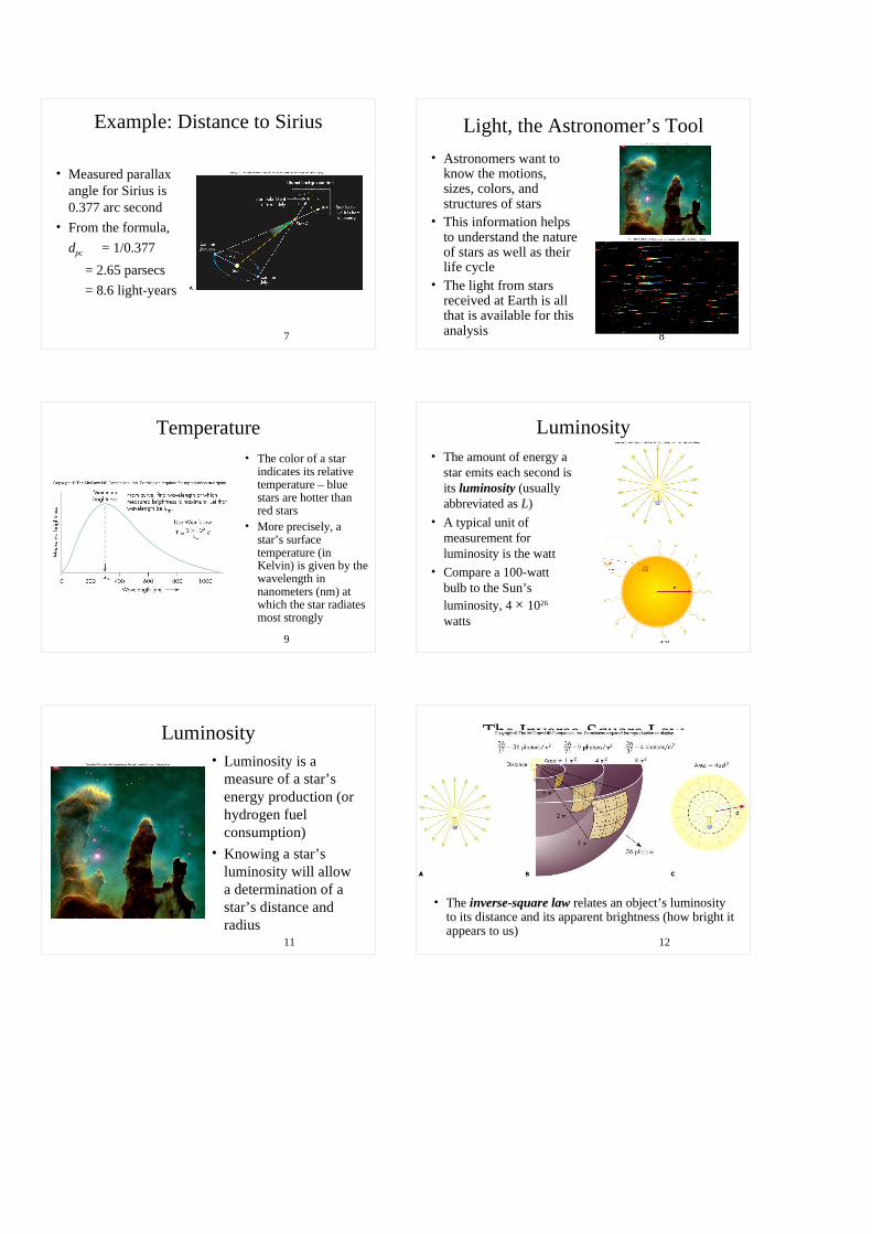
Example: Distance to Sirius

• Measured parallax angle for Sirius is 0.377 arc second

• From the formula,

dpc = 1/0.377

= 2.65 parsecs

= 8.6 light-years

8

Light, the Astronomer’s Tool

• Astronomers want to know the motions, sizes, colors, and structures of stars

• This information helps to understand the nature of stars as well as their life cycle

• The light from stars received at Earth is all that is available for this analysis

9

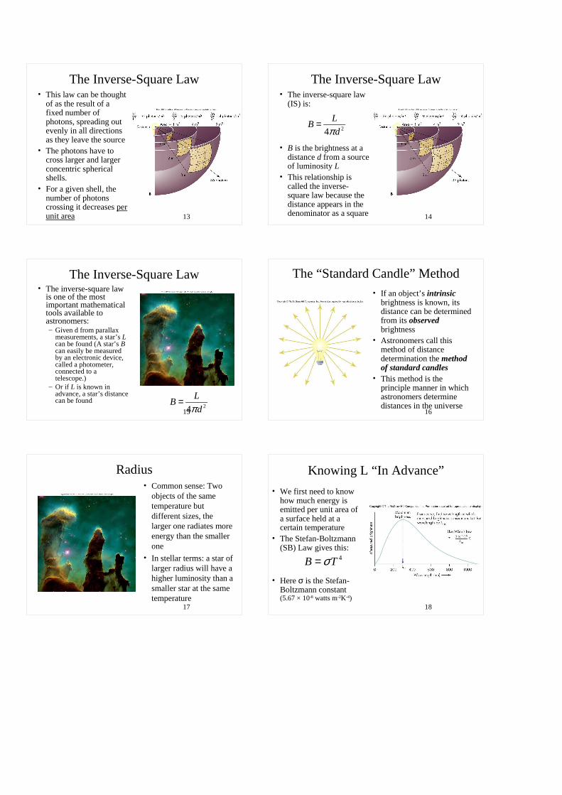
Temperature• The color of a star

indicates its relative temperature – blue stars are hotter than red stars

• More precisely, a star’s surface temperature (in Kelvin) is given by the wavelength in nanometers (nm) at which the star radiates most strongly

10

Luminosity• The amount of energy a

star emits each second is its luminosity (usually abbreviated as L)

• A typical unit of measurement for luminosity is the watt

• Compare a 100-watt bulb to the Sun’s luminosity, 4 × 1026 watts

11

Luminosity• Luminosity is a

measure of a star’s energy production (or hydrogen fuel consumption)

• Knowing a star’s luminosity will allow a determination of a star’s distance and radius

12

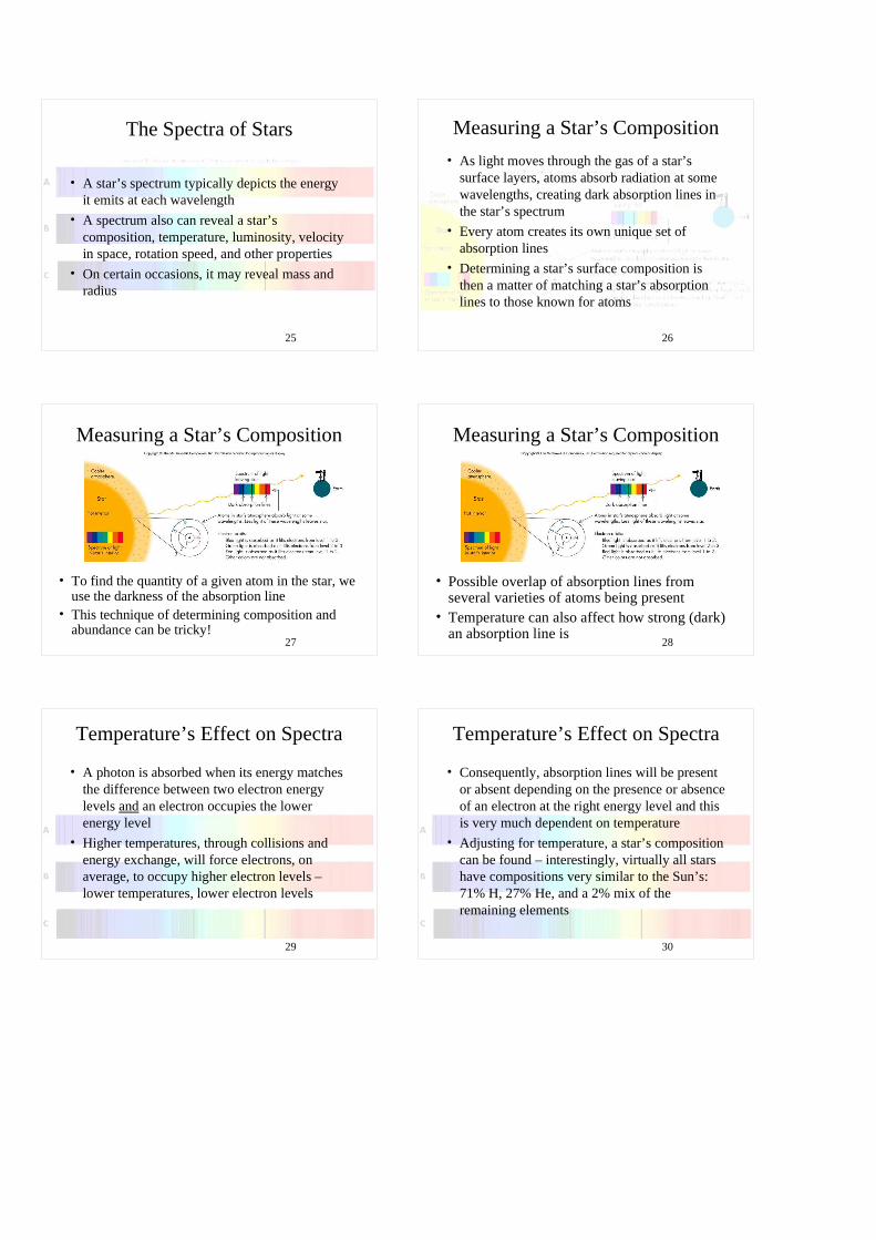
The Inverse-Square Law

• The inverse-square law relates an object’s luminosity to its distance and its apparent brightness (how bright it appears to us)

13

The Inverse-Square Law• This law can be thought

of as the result of a fixed number of photons, spreading out evenly in all directions as they leave the source

• The photons have to cross larger and larger concentric spherical shells.

• For a given shell, the number of photons crossing it decreases per unit area 14

• The inverse-square law (IS) is:

• B is the brightness at a distance d from a source of luminosity L

• This relationship is called the inverse-square law because the distance appears in the denominator as a square


24

LB

dπ=

15

• The inverse-square law is one of the most important mathematical tools available to astronomers:– Given d from parallax

measurements, a star’s L can be found (A star’s B can easily be measured by an electronic device, called a photometer, connected to a telescope.)

– Or if L is known in advance, a star’s distance can be found


24

LB

dπ=

16

The “Standard Candle” Method• If an object’s intrinsic

brightness is known, its distance can be determined from its observed brightness

• Astronomers call this method of distance determination the method of standard candles

• This method is the principle manner in which astronomers determine distances in the universe

17

• Common sense: Two objects of the same temperature but different sizes, the larger one radiates more energy than the smaller one

• In stellar terms: a star of larger radius will have a higher luminosity than a smaller star at the same temperature

Radius

18

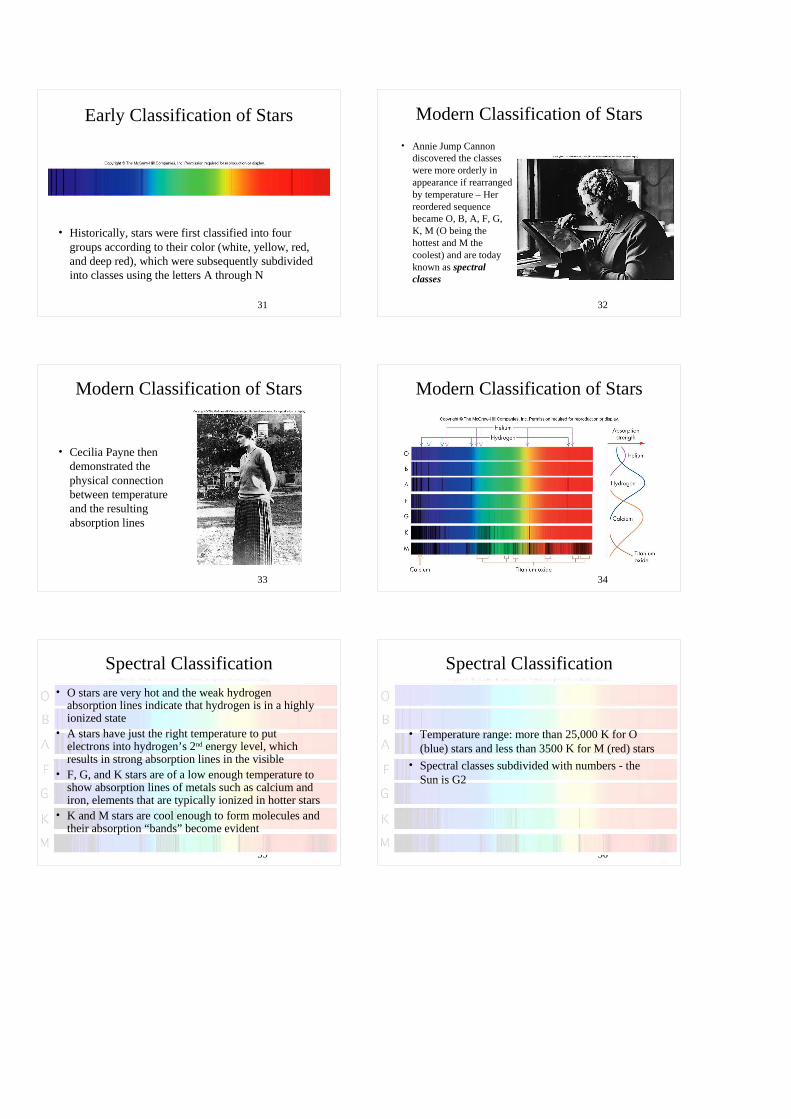
Knowing L “In Advance”

• We first need to know how much energy is emitted per unit area of a surface held at a certain temperature

• The Stefan-Boltzmann (SB) Law gives this:

• Here σ is the Stefan-Boltzmann constant (5.67 × 10-8 watts m-2K -4)

4B Tσ=

19

Tying It All Together• The Stefan-Boltzmann

law only applies to stars, but not hot, low-density gases

• We can combine SB and IS to get:

• R is the radius of the star • Given L and T, we can

then find a star’s radius!

2 44L R Tπ σ=

20

Tying It All Together

21

Tying It All Together• The methods using the

Stefan-Boltzmann law and interferometer observations show that stars differ enormously in radius– Some stars are hundreds of

times larger than the Sun and are referred to as giants

– Stars smaller than the giants are called dwarfs 2 44L R Tπ σ=

22

The Magnitude Scale• About 150 B.C., the Greek astronomer Hipparchus

measured apparent brightness of stars using units called magnitudes– Brightest stars had magnitude 1 and dimmest had

magnitude 6– The system is still used today and units of measurement are

called apparent magnitudes to emphasize how bright a star looks to an observer

• A star’s apparent magnitude depends on the star’s luminosity and distance – a star may appear dim because it is very far away or it does not emit much energy

23

The Magnitude Scale

• The apparent magnitude can be confusing– Scale runs “backward”: high magnitude = low

brightness– Modern calibrations of the scale create negative

magnitudes– Magnitude differences equate to brightness ratios:

• A difference of 5 magnitudes = a brightness ratio of 100

• 1 magnitude difference = brightness ratio of 1001/5=2.512

24

The Magnitude Scale

• Astronomers use absolute magnitude to measure a star’s luminosity– The absolute magnitude of a star is the apparent

magnitude that same star would have at 10 parsecs– A comparison of absolute magnitudes is now a

comparison of luminosities, no distance dependence

– An absolute magnitude of 0 approximately equates to a luminosity of 100L

�

25

The Spectra of Stars

• A star’s spectrum typically depicts the energy it emits at each wavelength

• A spectrum also can reveal a star’s composition, temperature, luminosity, velocity in space, rotation speed, and other properties

• On certain occasions, it may reveal mass and radius

26

Measuring a Star’s Composition

• As light moves through the gas of a star’s surface layers, atoms absorb radiation at some wavelengths, creating dark absorption lines in the star’s spectrum

• Every atom creates its own unique set of absorption lines

• Determining a star’s surface composition is then a matter of matching a star’s absorption lines to those known for atoms

27


• To find the quantity of a given atom in the star, we use the darkness of the absorption line

• This technique of determining composition and abundance can be tricky!

28


• Possible overlap of absorption lines from several varieties of atoms being present

• Temperature can also affect how strong (dark) an absorption line is

29

Temperature’s Effect on Spectra

• A photon is absorbed when its energy matches the difference between two electron energy levels and an electron occupies the lower energy level

• Higher temperatures, through collisions and energy exchange, will force electrons, on average, to occupy higher electron levels – lower temperatures, lower electron levels

30

Temperature’s Effect on Spectra

• Consequently, absorption lines will be present or absent depending on the presence or absence of an electron at the right energy level and this is very much dependent on temperature

• Adjusting for temperature, a star’s composition can be found – interestingly, virtually all stars have compositions very similar to the Sun’s: 71% H, 27% He, and a 2% mix of the remaining elements

31

Early Classification of Stars

• Historically, stars were first classified into four groups according to their color (white, yellow, red, and deep red), which were subsequently subdivided into classes using the letters A through N

32

Modern Classification of Stars

• Annie Jump Cannon discovered the classes were more orderly in appearance if rearranged by temperature – Her reordered sequence became O, B, A, F, G, K, M (O being the hottest and M the coolest) and are today known as spectral classes

33


• Cecilia Payne then demonstrated the physical connection between temperature and the resulting absorption lines

34


35

Spectral Classification

• O stars are very hot and the weak hydrogen absorption lines indicate that hydrogen is in a highly ionized state

• A stars have just the right temperature to put electrons into hydrogen’s 2nd energy level, which results in strong absorption lines in the visible

• F, G, and K stars are of a low enough temperature to show absorption lines of metals such as calcium and iron, elements that are typically ionized in hotter stars

• K and M stars are cool enough to form molecules and their absorption “bands” become evident

36

Spectral Classification

• Temperature range: more than 25,000 K for O (blue) stars and less than 3500 K for M (red) stars

• Spectral classes subdivided with numbers - the Sun is G2

37

Measuring a Star’s Motion• A star’s motion is determined from the

Doppler shift of its spectral lines– The amount of shift depends on the star’s

radial velocity, which is the star’s speed along the line of sight

– Given that we measure ∆λ, the shift in wavelength of an absorption line of wavelength λ, the radial speed v is given by:

– c is the speed of light

v cλ

λ∆ =

38

Measuring a Star’s Motion• Note that λ is the

wavelength of the absorption line for an object at rest and its value is determined from laboratory measurements on nonmoving sources

• An increase in wavelength means the star is moving away, a decrease means it is approaching – speed across the line on site cannot be determined from Doppler shifts v c

λλ

∆ =

39

Measuring a Star’s Motion• Doppler measurements and related analysis

show:– All stars are moving and that those near the Sun

share approximately the same direction and speed of revolution (about 200 km/sec) around the center of our galaxy

– Superimposed on this orbital motion are small random motions of about 20 km/sec

– In addition to their motion through space, stars spin on their axes and this spin can be measured using the Doppler shift technique – young stars are found to rotate faster than old stars

40

Binary Stars• Two stars that revolve around each other as a

result of their mutual gravitational attraction are called binary stars

• Binary star systems offer one of the few ways to measure stellar masses – and stellar mass plays the leading role in a star’s evolution

• At least 40% of all stars known have orbiting companions (some more than one)

• Most binary stars are only a few AU apart – a few are even close enough to touch

41

Visual Binary Stars

• Visual binaries are binary systems where we can directly see the orbital motion of the stars about each other by comparing images made several years apart

42

Spectroscopic Binaries

• Spectroscopic binaries are systems that are inferred to be binary by a comparison of the system’s spectra over time

• Doppler analysis of the spectra can give a star’s speed and by observing a full cycle of the motion the orbital period and distance can be determined

43

Stellar Masses

• Kepler’s third law as modified by Newton is

• m and M are the binary star masses (in solar masses), P is their period of revolution (in years), and a is the semimajor axis of one star’s orbit about the other (in AU)

2 3( )m M P a+ =

44

Stellar Masses

• P and a are determined from observations (may take a few years) and the above equation gives the combined mass (m + M)

• Further observations of the stars’ orbit will allow the determination of each star’s individual mass

• Most stars have masses that fall in the narrow range 0.1 to 30 M�

45

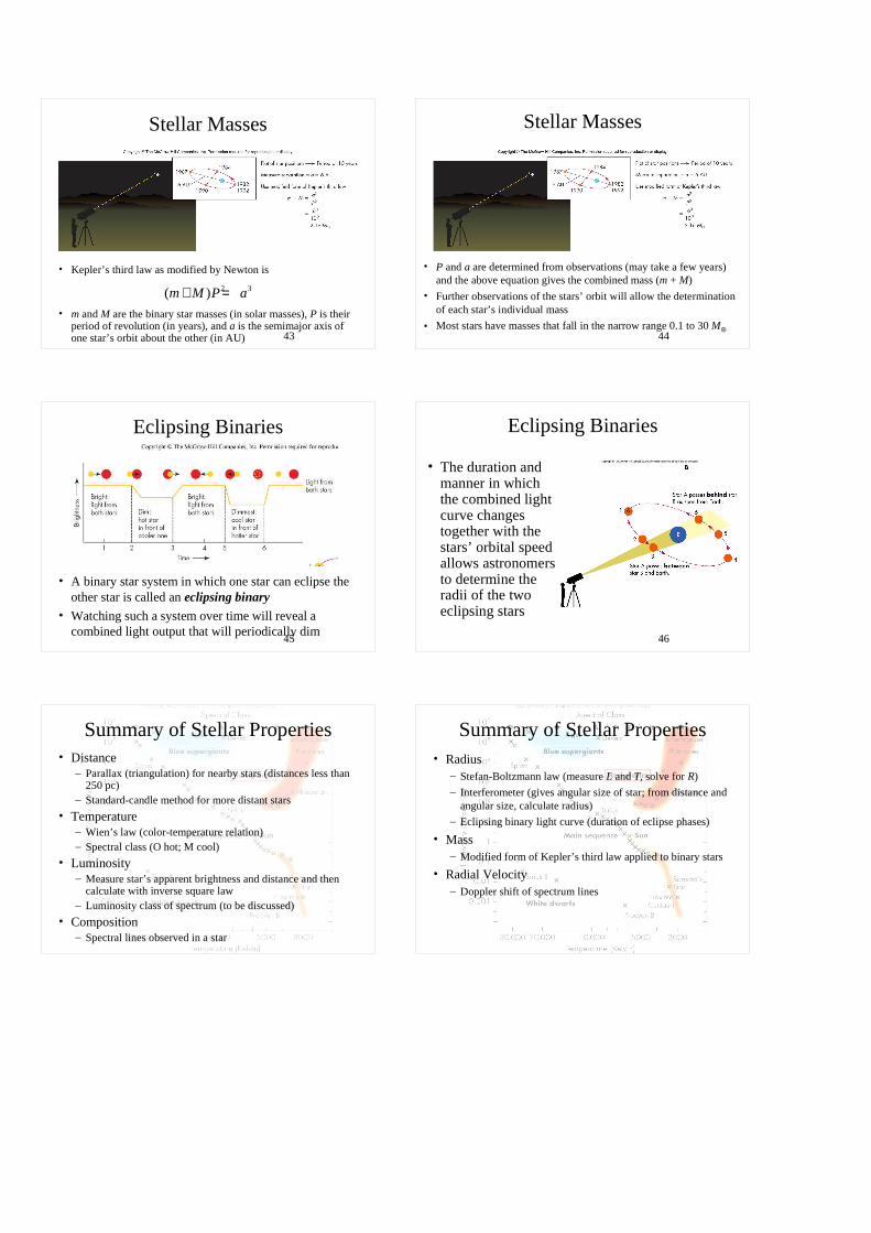
Eclipsing Binaries

• A binary star system in which one star can eclipse the other star is called an eclipsing binary

• Watching such a system over time will reveal a combined light output that will periodically dim

46

Eclipsing Binaries

• The duration and manner in which the combined light curve changes together with the stars’ orbital speed allows astronomers to determine the radii of the two eclipsing stars

47

Summary of Stellar Properties• Distance

– Parallax (triangulation) for nearby stars (distances less than 250 pc)

– Standard-candle method for more distant stars

• Temperature– Wien’s law (color-temperature relation)– Spectral class (O hot; M cool)

• Luminosity– Measure star’s apparent brightness and distance and then

calculate with inverse square law– Luminosity class of spectrum (to be discussed)

• Composition– Spectral lines observed in a star 48

Summary of Stellar Properties• Radius

– Stefan-Boltzmann law (measure L and T, solve for R)

– Interferometer (gives angular size of star; from distance and angular size, calculate radius)

– Eclipsing binary light curve (duration of eclipse phases)

• Mass– Modified form of Kepler’s third law applied to binary stars

• Radial Velocity– Doppler shift of spectrum lines

49

Putting it all together – The Hertzsprung-Russell Diagram

• So far, only properties of stars have been discussed – this follows the historical development of studying stars

• The next step is to understand why stars have these properties in the combinations observed

• This step in our understanding comes from the H-R diagram, developed independently by Ejnar Hertzsprung and Henry Norris Russell in 1912

50

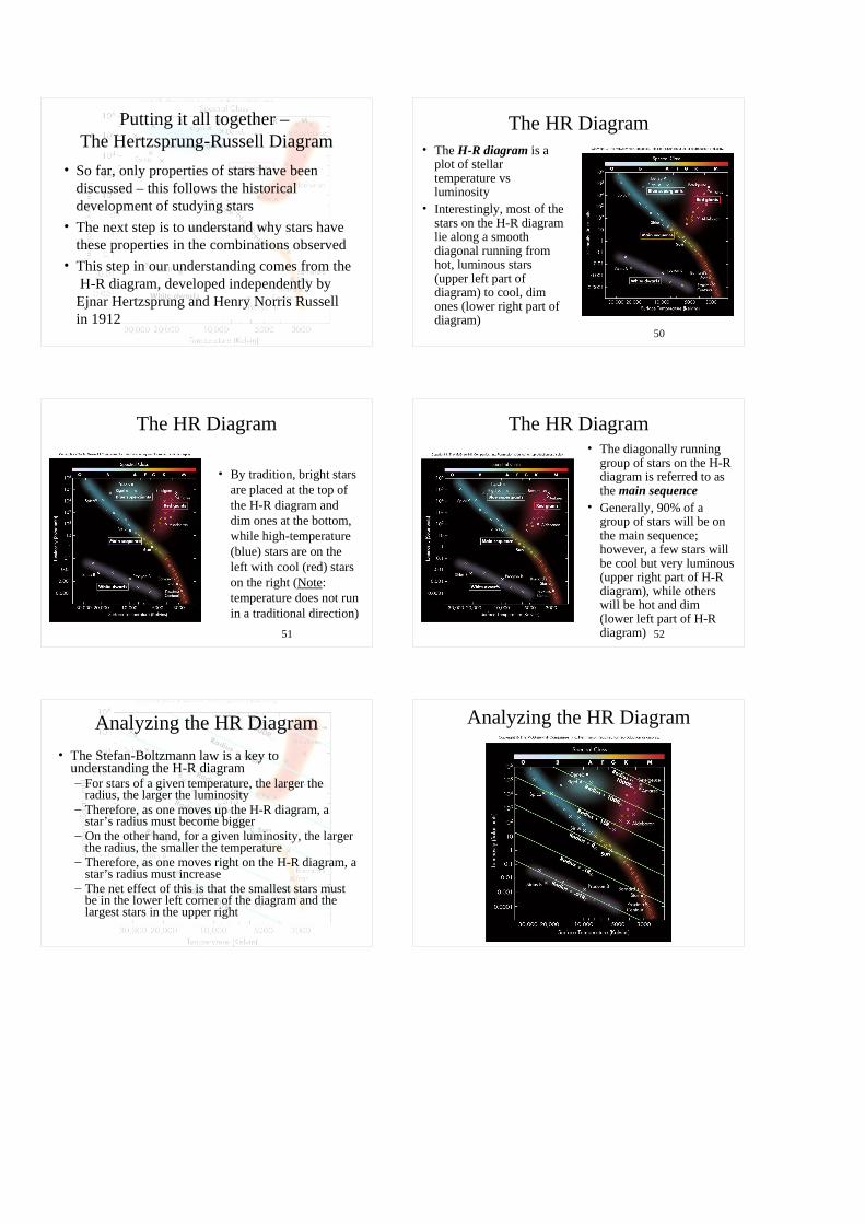
The HR Diagram• The H-R diagram is a

plot of stellar temperature vs luminosity

• Interestingly, most of the stars on the H-R diagram lie along a smooth diagonal running from hot, luminous stars (upper left part of diagram) to cool, dim ones (lower right part of diagram)

51

The HR Diagram

• By tradition, bright stars are placed at the top of the H-R diagram and dim ones at the bottom, while high-temperature (blue) stars are on the left with cool (red) stars on the right (Note: temperature does not run in a traditional direction)

52

The HR Diagram• The diagonally running

group of stars on the H-R diagram is referred to as the main sequence

• Generally, 90% of a group of stars will be on the main sequence; however, a few stars will be cool but very luminous (upper right part of H-R diagram), while others will be hot and dim (lower left part of H-R diagram)

53

Analyzing the HR Diagram

• The Stefan-Boltzmann law is a key to understanding the H-R diagram– For stars of a given temperature, the larger the

radius, the larger the luminosity– Therefore, as one moves up the H-R diagram, a

star’s radius must become bigger– On the other hand, for a given luminosity, the larger

the radius, the smaller the temperature– Therefore, as one moves right on the H-R diagram, a

star’s radius must increase– The net effect of this is that the smallest stars must

be in the lower left corner of the diagram and the largest stars in the upper right

54

Analyzing the HR Diagram

55

Giants and Dwarfs

• Stars in the upper left are called red giants (red because of the low temperatures there)

• Stars in the lower right are white dwarfs

• Three stellar types: main sequence, red giants, and white dwarfs

56

Giants and Dwarfs

• Giants, dwarfs, and main sequence stars also differ in average density, not just diameter

• Typical density of main-sequence star is 1 g/cm3, while for a giant it is 10-6 g/cm3

57

• Main-sequence stars obey a mass-luminosity relation, approximately given by:

• L and M are measured in solar units

• Consequence: Stars at top of main-sequence are more massive than stars lower down

The Mass-Luminosity Relation

3L M=

58

Luminosity Classes

• Another method was discovered to measure the luminosity of a star (other than using a star’s apparent magnitude and the inverse square law)– It was noticed that some stars had very narrow

absorption lines compared to other stars of the same temperature

– It was also noticed that luminous stars had narrower lines than less luminous stars

• Width of absorption line depends on density: wide for high density, narrow for low density

59

Luminosity Classes

60

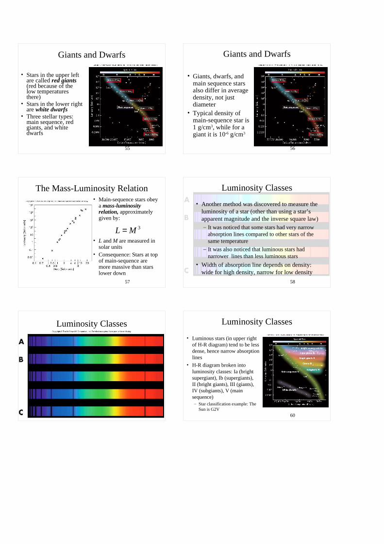
Luminosity Classes

• Luminous stars (in upper right of H-R diagram) tend to be less dense, hence narrow absorption lines

• H-R diagram broken into luminosity classes: Ia (bright supergiant), Ib (supergiants), II (bright giants), III (giants), IV (subgiants), V (main sequence)– Star classification example: The

Sun is G2V

61

Summary of the HR Diagram• Most stars lie on the main

sequence– Of these, the hottest stars

are blue and more luminous, while the coolest stars are red and dim

– Star’s position on sequence determines its mass, being more near the top of the sequence

• Three classes of stars:– Main-sequence– Giants– White dwarfs

62

Variable Stars

• Not all stars have a constant luminosity – some change brightness: variable stars

• There are several varieties of stars that vary and are important distance indicators

• Especially important are the pulsating variables – stars with rhythmically swelling and shrinking radii

63

Mira and Cepheid Variables

• Variable stars are classified by the shape and period of their light curves – Mira and Cepheid variables are two examples 64

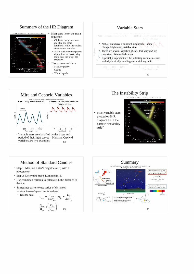
The Instability Strip

• Most variable stars plotted on H-R diagram lie in the narrow “instability strip”

65

Method of Standard Candles• Step 1: Measure a star’s brightness (B) with a

photometer• Step 2: Determine star’s Luminosity, L• Use combined formula to calculate d, the distance to

the star• Sometimes easier to use ratios of distances

– Write Inverse-Square Law for each star

– Take the ratio:2 2

2

,4 4

farnearnear far

near far

farnear

far near

LLB B

d d

dB

B d

π π= =

= 66

Summary

Documents

Triangulation Trigonometric Parallax