TRENDS IN REGIONAL EVAPOTRANSPIRATION ACROSS THE …

Pre-print � In review for publication in Water Resources Research

1

Trends in Regional Evapotranspiration across the United States under the Complementary Relationship Hypothesis

MICHAEL T. HOBBINS1 AND JORGE A. RAMÍREZ1

Civil Engineering Department, Colorado State University, Fort Collins, CO.

THOMAS C. BROWN2 Rocky Mountain Research Station, U. S. Forest Service,Fort Collins, CO.

Abstract

The hypothesis of a complementary relationship in regional evapotranspiration allows for estimation of actual evapotranspiration on a regional scale by simple, physically based models that take into account feedbacks in land surface-atmosphere dynamics. A regional, seasonal Advection-Aridity model is used to create a spatially distributed, monthly time-series of actual evapotranspiration for a period of 27 years at a 5-km resolution over the conterminous United States. For the conterminous United States as a whole, a 4.3% increase in annual actual evapotranspiration over the period WY 1962-1988 was observed, a trend that was significant at the 90% confidence level according to the Mann-Kendall test. Trends in annual evapotranspiration are analyzed across the spatial scales of the continental United States, a Water Resources Region (WRR), a river basin of 16,000 km2, and an individual 5-km square cell. Reducing the spatial scale allowed for clearer identification of areas with significant trends. To establish a base-line for the study of climate change and/or variability, a methodology for rigorous examination of past trends in actual evapotranspiration is proposed, wherein such trends are broken down into the climatic components of actual evapotranspiration in the context of the complementary relationship, and no assumptions are made about the temporal stationarity of the net available energy. Trends in actual evapotranspiration can thus be determined to originate in either the energy budget or the water budget, or both. Keywords Evapotranspiration, Solar radiation, Advection, Energy budget, Water yield, Wind speed, Vapor pressure, Complementary relationship, Advection-Aridity, Climate change

1. Introduction

Climatic change and variability will have myriad effects on our lives, none more immediate than those involving the hydrologic cycle. In modeling these effects at the watershed-scale, actual evapotranspiration (ETa) is the component of the hydrologic cycle that presents the greatest challenge. It is also one of the most sensitive components to climate change and variability. In order to understand the effects of an anthropogenically altered hydrosphere, hydrologists and water managers are increasingly turning their attention to climate models, but it is essential first to establish a base-line for such modeling, by rigorously examining past change and/or variability.

There is a dearth of direct analysis of ETa, and especially of trend analyses of ETa. The vast majority of hydrological studies of climate change and variability has concentrated on the directly observable components of the hydrologic cycle, namely precipitation [e.g., Karl and Knight, 1998] and streamflow [e.g., Wahl, 1992; Chiew and McMahon, 1996; Lins, 1997; Lins 1 Water Resources, Hydrologic and Environmental Sciences Division

Civil Engineering Department Colorado State University, Fort Collins, CO 80523


2

and Slack, 1999]. Even those studies that take a more holistic hydrological approach�whether it be an examination of indices of climate change over the conterminous United States [Karl et al., 1996]; of long-term hydroclimatological trends over the same region [Lettenmaier et al., 1994]; or of the effects of climate change on the hydrology of a smaller, WRR-scale basin [Westmacott and Burn, 1997]�do not examine trends in ETa. Typically, when evapotranspiration has been studied, it has been in the context of potential evapotranspiration (ETp) at a point [Lockwood, 1994], usually based on observations at evaporation pans [Eitzinger et al., personal communication, 2001], and not ETa at a regional scale. Although such studies are of interest in the context of trends in the standard agrometeorological variables, wherein ETa is taken to be a function of ETp determined by coefficients describing local crop and soil moisture conditions, they neglect the complementarity of ETa and ETp evident at the regional scale.

The primary reasons for the lack of direct analysis of ETa are the difficulties inherent in measuring ETa and the complications of scale. In the study of evapotranspiration (ET), the physics of energy and mass transfer at the land surface-atmosphere interface can be successfully modeled at small temporal and spatial scales [Katul and Parlange, 1992; Parlange and Katul, 1992a; Parlange and Katul, 1992b], but our understanding of these processes at the larger (e.g., basinwide) scale necessary for use by hydrologists, water managers, and climate and ecological modelers is limited. Consequently, our ability to estimate regional evapotranspiration is often constrained by models that treat ETp as an independent climatic forcing process and derive ETa estimates through non-physical, locally parameterized relationships thereof.

ETa is generally modeled either as a simple, often empirical function of pan evaporation observed at nearby weather stations, or by ground-based models that rely on gross assumptions regarding processes in the poorly understood soil, vegetative, and atmospheric systems, while ignoring the many feedback mechanisms and interactions that occur at the interfaces between the three [Morton, 1983]. Vegetation is generally assumed to act as a �passive wick,� thereby ignoring physiologic feedback loops at the vegetation-atmosphere interface that respond to increases in the vapor pressure deficit of the ambient air�and corresponding increases in ETp�by reducing the actual transpiration rate [Morton, 1983]. Most importantly, with regard to the atmospheric assumptions of the soil-plant-atmosphere system, ETp is traditionally assumed to be independent of ETa and is used to reflect evaporation demand. It is often calculated by approximate solutions such as the Penman equation.

These assumptions about the nature of moisture dynamics in each of the components of the land surface-atmosphere interface point to the need for models of regional evapotranspiration that consider the evaporative system as an integrated whole, that bypass the poorly understood dynamics within each component, and that incur minimal data requirements about the nature of the land surface. Complementary relationship models are such models.

The advantages to hydrologists of complementary relationship models are as follows: (i) they can accurately predict ETa over regional extents, as indicated by the near-zero mean annual error for the Advection-Aridity model reported in Hobbins et al., [2001b]; (ii) they implicitly account for the soil moisture-dependence of ETp and bypass complex and poorly understood soil-plant processes, thereby obviating the need for locally optimized coefficients and surface parameterizations of soil moisture or stomatal resistance; (iii) they rely solely on routine climatological observations; and (iv) they allow the estimation of ET over large-scale land surfaces without a priori knowledge of the nature of the land surface, beyond that it may be assumed to be homogeneous at scale lengths conducive to boundary layer mixing. It is for these reasons that Hobbins et al. [2001c] state that for hydrologists working in large-scale homogenous


3

areas, these complementary relationship models are preferred over traditional evapotranspiration models using land-based parameterizations, as the input data are distributed and reflect surface conditions regardless of the origins of the water and degree of anthropogenic disturbance.

Analyses of trends in ETa are sorely needed. Such analyses would aid water managers attempting to resolve issues of water supply and demand in increasingly variable hydroclimatic conditions. The first attempts to determine large scale trends in ETa were published by Szilagyi [2001] and Szilagyi et al. [2001], who estimated long-term trends in regional ETa across the conterminous United States using the complementary relationship. Their work shows the potential of complementary relation models for determining trends in ETa. However, we suggest that their use of evaporation pan observations (ETpan) as predictors of ETp limits the accuracy of trend analyses of ETa. Hobbins et al. [2001b] list four primary reasons why this assumption is problematic: (i) the heterogeneity of the reach upwind of the evaporation pan may confound the presumed complementarity of ETa and ETpan; (ii) changes in land-use upwind of the pan will affect the ETpan record; (iii) there is often significant spatial disjoint between evaporation pans (such as those producing the data reported by Peterson et al. [1995]) and the stations where the meteorological data are gathered; and (iv) there are clear spatial and seasonal biases in the national ETpan record.

We examine trends in a spatially distributed, long-term time-series of ETa across the conterminous United States derived from the seasonally and regionally enhanced Advection-Aridity model of the complementary relationship in regional ETa of Hobbins et al., [2001b]. The Advection-Aridity model is one of the most common complementary relationship formulations and was first proposed by Brutsaert and Stricker [1979]. It has since been reparameterized on a regional and seasonal basis by the authors [Hobbins et al., 2001b]. The model combines the effects of regional advection on ETp with the hypothesis of a complementary relationship between ETp and ETa, and is described in the following section.

In this study, we generated surfaces of solar radiation, wind speed, average temperature, humidity, albedo, and elevation at every 5 km x 5 km pixel for the entire conterminous United States, through spatial interpolation from all available stations in each input variable network. Using these spatially distributed fields, we may represent trends in evapotranspiration at any spatial breakdown desired: water resource regions (WRRs), states, climatic divisions, specific watersheds, or physiographic regions. Further, we examine the input climatic variables for long-term trends, avoiding any assumptions of stationarity in any component of ETa, specifically the net available energy, Qn.

The utility and scientific merits of complementary relationship models have been shown by numerous studies [Morton, 1965, 1975, 1976a, 1976b, 1978, 1983; Brutsaert and Stricker, 1979]. More recent studies [Hobbins et al., 1999, 2001a, 2001b] have tested two applications of the hypothesis�the CRAE model and a regionally and seasonally reparameterized Advection-Aridity model�in scores of basins across a wide range of climatic regimes, and have reported the predictive power of the model increasing moving towards regions of climate control of evapotranspiration rates, (i.e., errors in closing the long-term, large-scale water balances converge towards zero with increasing humidity), and generally decreasing towards regions of increasing soil control, (i.e., errors increase, in both scale and variability, with increasing aridity). Notwithstanding this climatic sensitivity, the near-zero mean error of the improved seasonal, regional Advection-Aridity model used here indicates the utility of complementary relationship models in general, and the Advection-Aridity model in particular, for providing independent estimates of ETa.


4

2. THE REGIONAL-SEASONAL ADVECTION-ARIDITY MODEL OF THE COMPLEMENTARY RELATIONSHIP

The theory of the complementary relationship in regional evapotranspiration, first proposed by Bouchet [1963], considers ETp to be a function of the aforementioned feedback processes between limitations of water availability at the land surface and the evaporative power of the overlying atmosphere, while avoiding the difficulties inherent in coupling surface and free atmosphere phenomena in the soil-plant-atmosphere system. In modeling the complementary relationship, ETa is estimated using only data that describe the conditions of the over-passing air and no locally optimized coefficients are necessary.

The hypothesis of a complementary relationship states that over areas of a regional scale and away from any sharp environmental discontinuities, there exists a feedback mechanism between actual and potential evapotranspiration rates [Bouchet, 1963]. This relationship is described by equation (1):

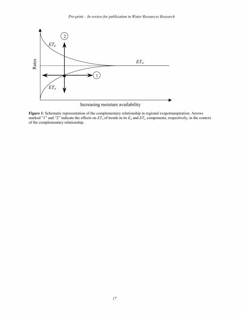
wpa kETETET =+ . (1) In homogeneous regions where the assumptions of a well-mixed atmospheric boundary layer and negligible upwind edge-effects hold well, all the energy at the surface that, due to limited water availability, is not taken up in the process of ETa increases the temperature and humidity gradients of the over-passing air and leads to an increase in ETp equal in magnitude to the decrease in ETa. Thus, under such conditions, the value of k is taken to equal 2. Under conditions where ETa equals ETp, this rate is referred to as the wet environment evaporation (ETw). Figure 1 illustrates the complementary relationship.

The Advection-Aridity model of the complementary relationship is described in detail by Brutsaert and Stricker [1979] and Hobbins et al. [2001b]. We summarize the model here. In this model, ETp is calculated by combining information from the energy budget and water vapor transfer in the Penman equation, shown below in equation (2), and ETw is calculated based on derivations of the concept of equilibrium evapotranspiration under conditions of minimal advection, first proposed by Priestley and Taylor [1972], and shown in equation (5). ETa is then calculated as a residual of equation (1).

The familiar expression of the Penman equation for ETp is:

anp EQETγ

γλγ

λ+∆

++∆∆= (2)

where λ represents the latent heat of vaporization, ∆ is the slope of the saturated vapor pressure curve at air temperature, γ is the psychrometric constant, and Qn is the net available energy at the surface. The second term of this combination approach represents the effects of large-scale advection in the mass transfer of water vapor, and takes the form of a scaled factor of an aerodynamic vapor transfer term Ea. Ea, also known as the �drying power of the air,� is a product of the vapor pressure deficit and a �wind function� of the speed of the advected air f(Ur), of the form (3):

( )( )aara eeUfE −= * . (3)


5

In equation (3), Ur represents the wind speed observed at r meters above the evaporating

surface, and ea* and ea are the saturation vapor pressure and the actual vapor pressure of the air at

r meters above the surface, respectively. Previous work by the authors with the Advection-Aridity model [Hobbins et al., 1999,

2001a, 2001b] has shown that performance of the original model is strongly biased with respect to the advective input, and that this bias may be removed by proper selection of the wind function f(Ur).

The wind function f(Ur) is either theoretically or empirically derived. Theoretical expressions for the wind function under neutral conditions�i.e., under a stable atmospheric boundary layer�are available. While much work has been done in the agricultural arena to calibrate or reformulate wind functions for use in the combination or Penman equation (2) (e.g., Allen [1986], Van Bavel [1966], Wright [1982]), these formulations operate on a limited spatial and temporal scale, do not hypothesize feedbacks of a regional nature, and require local parameterizations of resistance and canopy roughness. Thus, they are not applicable in predicting regional evapotranspiration. Further, in the context of modeling monthly regional ETa with the complementary relationship, the effects of atmospheric instability and the onerous data requirements rule out theoretical formulations. In reparameterizing and recalibrating the Advection-Aridity model on a regional, seasonal basis across the conterminous United States, Hobbins et al. [2001b] suggested an empirical linear approximation for f(Ur), of the form (4):

( ) ( ) 2,,,2 UbaUfUf jijijir +=≈ (4) where U2 is mean monthly wind speed at 2 meters above the ground, and the indices i and j represent the month and Water Resource Region (WRR) of application.

The Advection-Aridity model calculates ETw using the Priestley and Taylor [1972] partial equilibrium evaporation equation (5):

nw QETγ

αλ+∆∆= . (5)

The value of the Priestley-Taylor coefficient α has been the subject of much discussion for various land-cover types and at a range of temporal scales. For example, values of 1.05 [McNaughton and Black, 1973] to 1.32 [Morton, 1983] have been suggested based on short, well-watered Douglas fir and on Morton�s [1983] re-examination of the seminal work by Priestley and Taylor [1972], respectively, while at a range of temporal scales, seasonal values of 1.15 to 1.50 and intra-daily values of between 1.15 and 1.42 have been proposed by DeBruin and Keijman [1979]. Recognizing the variability in estimates for this empirical parameter, its calibration was the focus of much of the work in Hobbins et al. [2001b], wherein a value of 1.3177 was shown to remove a consistent bias towards underestimation of ETa across a set of 139 basins in the conterminous United States. This value of α (1.3177), which is close to the value (α = 1.32) predicted by Morton [1983] in his re-assessment of results reported by Priestley and Taylor [1972], is used in this study.

Combining the expressions for the wind function f(Ur) (4), the drying power of the air Ea (3), potential evapotranspiration ETp (2), and wet environment evaporation ETw (5) into the


6

expression of the complementary relationship (1), and rearranging terms yields the following expression for ETa (6):

( ) ( )( )aajijina eeUbaQkET −++∆

−+∆∆−= *

2,,1γ

γλγ

αλ (6)

where the first term on the right represents the influence of the energy budget, and the second term the local wetness.

In reparameterizing the wind function f(U2)i,j on a regional and seasonal basis and recalibrating the Priestley-Taylor coefficient α, Hobbins et al. [2001b] reduced the mean annual closure error for large-scale, long-term water budgets across the conterminous United States from 7.92% of precipitation to 0.39%. We have since re-examined the applicability of the value of k = 2 for estimating regional ETa under non-ideal conditions where the complementary relationship�s main assumption�that over regional-scale evaporating surfaces that are homogeneous with regard to topography and moisture availability, all net available energy not expended in evapotranspiration goes to increasing potential evapotranspiration�is questionable. As a result, in this analysis, a value of k = 1.946 is applied across areas of rugged terrain, i.e., those areas to the west of the Continental Divide (WRRs 14 through 18). 3. METHODOLOGY AND DATA SETS

To produce a spatially distributed ETa time series, the Advection-Aridity model as formulated by the authors requires input data on solar radiation, wind speed, average temperature, humidity, albedo, and elevation. Solar radiation data were drawn from 216 stations in the �Solar and Meteorological Surface Observation Network (SAMSON)� [NOAA, 1993]. The solar radiation input for the derivation of Qn was the sum of diffuse radiation and topographically corrected direct radiation. Wind speed data were drawn from 246 stations in the SAMSON [NOAA, 1993] and �U.S. Environmental Protection Agency Support Center for Regulatory Air Models (EPA-SCRAM)� networks. Temperature data were drawn from 8330 stations in �NCDC Summary of the Day� [EarthInfo, 1998a], and average temperature was estimated as the mean of the average monthly maximum and average monthly minimum temperatures. Humidity data, in the form of dew-point temperatures, were drawn from 320 stations in �NCDC Surface Airways� [EarthInfo, 1998b]. Average monthly albedo surfaces based on AVHRR data were taken from Gutman [1988]. The elevation data were extracted from a 30-arc-second DEM.

In order to generate areal ETa coverages, spatial interpolation techniques were applied to the point observations of the input variables. All spatial interpolation and analyses were conducted at a 5-km cell size for the conterminous United States. Spatial interpolation procedures are detailed in Hobbins et al. [2001a]. As reported in Hobbins et al. [1999, 2001a, 2001b], the model is climatically robust and spatially distributed, and it is thereby able to render estimates of ETa that are constrained at the upper end of spatial resolution only by computational burdens and data availabilities, and at the lower end by the physics of the processes themselves.

The period of study was water years 1962-1988. At each 5 km x 5 km cell across the conterminous United States, monthly volumes of ETa and its components Ea and ETw were computed for this 27-year period. Time series for each month and for annual totals were then tested for trends using the non-parametric Mann-Kendall test, which is commonly used with hydrologic time series [Lettenmaier et al., 1994]. The Mann-Kendall statistic is given by (7):


7

( )∑ ∑−

= +=

−=1

1 1

sgnn

k

n

kjkj xxS (7)

where n is the length of the time series xi...xn, and sgn(·) is the sign function. The expected value and variance of S are given by (8) and (9), respectively:

[ ] 0=SE (8) ( ) ( )( ) ( )( )[ ] 18521521 ∑ +−−+−=

ttttnnnSVar (9)

where the second term represents an adjustment for tied or censored data. The test statistic Z is then given by (10):

( )

( )

<+=

>−

=

0100

01

SifSVar

SSif

SifSVar

S

Z . (10)

As a non-parametric test, no assumptions about the underlying distribution of data are

necessary. The test statistic Z is then used to test the null hypothesis that the data are identically distributed random observations without time-dependence. The null hypothesis cannot be rejected at the α-significance level if the following condition (11) applies:

21 α−< UZ (11) where U1-α/2 is the 1-α/2 quantile of the standard normal distribution. Otherwise, the null hypothesis must be rejected at the α-significance level in favor of the alternative hypothesis of a positive trend if the Z exceeds the critical value of U in a positive direction, and vice versa. The confidence level for this study was set at 95%, yielding a critical value of |Z| of 1.96. We present maps showing areas of significant trends, and, for informational purposes, non-significant trends as well.

It should be noted that the Mann-Kendall test statistic is non-dimensional, which is to say that it does not offer any quantification of the magnitude of the trend in the units of the time series under study, but is rather a measure of the correlation of xi with time and, as such, simply offers information as to the direction and a measure of the significance of any observed trend. 4. RESULTS

Temporal trends in hydrologic variables may occur and be studied at various spatial scales. For example, at the global or continental scale, warming as a result of the greenhouse effect may affect all aspects of the hydrologic cycle, with the primary effect that of the rising mean temperature resulting in a more energetic hydrologic cycle. At the WRR-scale, effects on the hydrologic cycle may run from modifications of weather patterns, such as deviation of storm tracks, to the effects of land-use changes, such as increased latent heat flux and humidity from


8

large-scale irrigation. These effects may be manifested in the short term�in anthropogenic migrations of agriculture, for example�and in the long term�as natural migrations of vegetative species in response to changes in moisture availability that result from changes in precipitation intensity, totals, and seasonality, and temperature effects on evapotranspiration. At the basin-scale (for example, the 16,000 km2 Rio Puerco basin discussed later), the effects on trends in the water yield function�which includes contributions from both surface and groundwater flow and may be estimated by the observed streamflow in the manner of Eagleson [1978]�may be difficult to detect, as the integrative dynamics of the component basin processes may average such effects out. Analyses of the components themselves�precipitation and evapotranspiration�may therefore be more instructive. At this scale, these include the direct effects of temperature on ETa, which may be readily modeled by use of regional ET models, and by the local variations in the dynamics of the hydrologic cycle, which may include changes in storages, the seasonality of precipitation, and in vegetation type and cover. With the variety of possible scales of responses in mind, we present results at a variety of spatial and temporal scales: from continental-scale, through WRR-scale, to the scale of a single 16,000 km2 basin, and for both annual and seasonal temporal scales.

The overall picture of trends in ETa across the conterminous United States over the period 1962-1988 is presented first. Then the trends of the two components of ETa�the radiative budget (here represented by ETw) and the mass transfer component (here represented by Ea)�are examined in the context of the complementary relationship. They are presented spatially across the extent of the study area and for a particular WRR. Finally, a comparison of average and pixel-specific annual and monthly trends with other surface components of the hydrologic cycle is made for a basin within that WRR. Continental-scale analysis

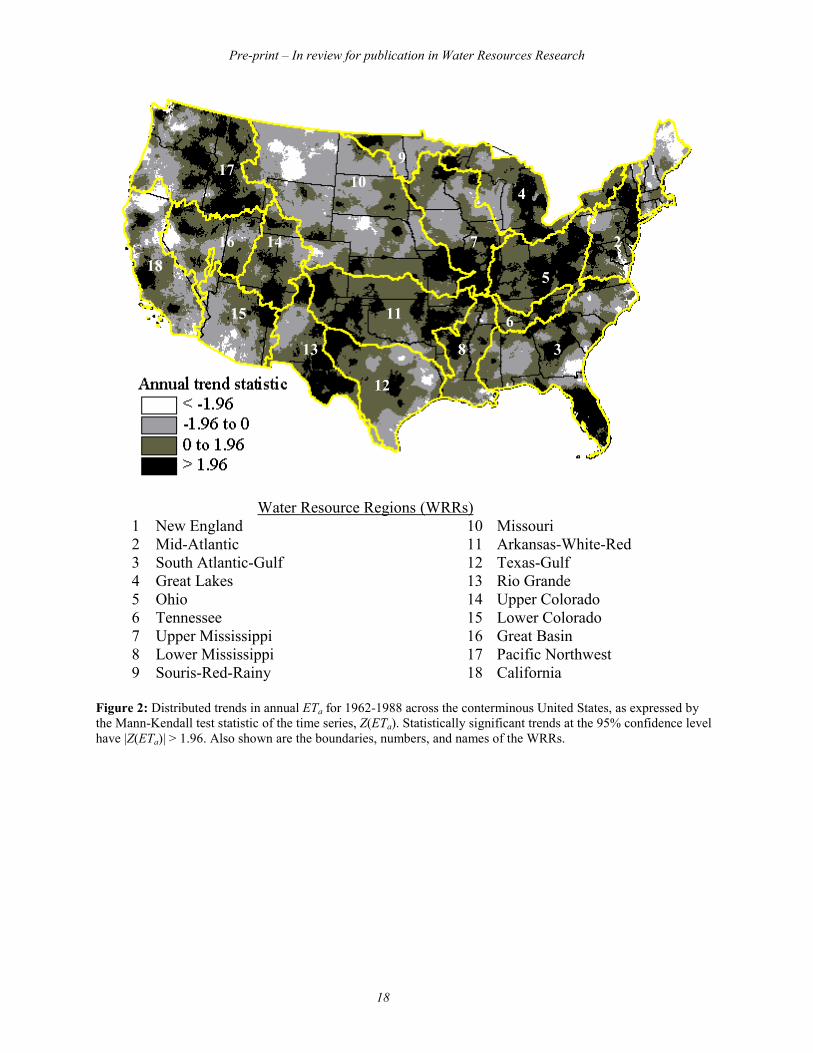
Figure 2 presents the larger picture: that of the distribution of ETa trends across the conterminous United States. By area, 3.5% shows statistically significant decreasing ETa; 27.6% shows statistically insignificant decreases in ETa; 45.9% shows statistically insignificant increases in ETa; and 23.0% shows statistically significant increases in ETa. Figure 2 reveals a complex distribution, with no continental-scale patterns emerging. The largest areas of significantly decreasing trends in ETa are found in Georgia, Texas, Nebraska, Montana, Nevada, California, and Oregon. Large areas of significantly increasing ETa are numerous, but are scattered over much of the United States; the largest concentrations are found in WRRs 2 (Mid-Atlantic), 3 (South Atlantic-Gulf), 5 (Ohio), 6 (Tennessee), 11 (Arkansas-White-Red), 13 (Rio Grande), 14 (Upper Colorado), and 17 (Pacific Northwest). The non-homogeneity of these trends at the continental scale and even within specific WRRs is in part the result of the fact that neither the conterminous United States nor the constituent WRRs are climatologically homogeneous regions. For instance, WRR 11 (Missouri) includes both the Rocky Mountains at the Continental Divide on the Idaho-Montana border and vast tracts of the High Plains, extending as far southeast as the Mississippi River on the Missouri-Illinois border. Examining results from such a large and hydrologically diverse single region may not be a useful tool and may instead have the effect of rendering useful data into mere noise.

We quantified these trends by generating trend slopes for the ETa time series at each 5 km x 5 km pixel and then spatially averaging these trend-slopes across the continental United States. The resultant trend is a 4.3% increase in ETa across the conterminous United States over the


9

period WY 1962-1988, a trend with a Mann-Kendall test statistic of 1.63, indicating statistical significance at the 90% confidence level. This may be compared to the result of Szilagyi [2001], who reported a 2.5% increase in annual ETa over the period 1961-1990, and who, in a follow-up paper [Szilagyi et al., 2001] conclude that their complementary relationship model overestimates trends in ETa. The difference in results may relate to the difference in methodology: our results were derived from a model that is both spatially distributed and well-calibrated; and we did not rely on continental-scale spatial averaging from station-values of ETa, as did Szilagyi [2001] and Szilagyi et al. [2001], who used 210 and 132 stations, respectively. As mentioned earlier, our model achieved near zero closure errors (i.e., 0.39% of annual precipitation) for long-term water balances that represented a wide spectrum of basin-sizes and climatic regimes across the conterminous United States [Hobbins et al., 2001b]. Decomposition of Observed Trends

Having examined the overall picture of trends in ETa, we turn to a first-order determination of what drives these trends. The temporal trend of ETa may be obtained by substituting equation (2) and equation (5) into equation (1) and differentiating with respect to time. This yields the following equation:

dtQd

QET

dtEd

EET

dtETd n

n

aa

a

aa

∂∂

+∂

∂= , (12)

where <.> represents the temporal averaging over the length of the time period. Equation (12) shows that trends in ETa can be the result of trends in both Qn (the net available energy for evaporation) and Ea (the drying power of the air). Thus, we report on trends in both these components, where Qn is examined through ETw.

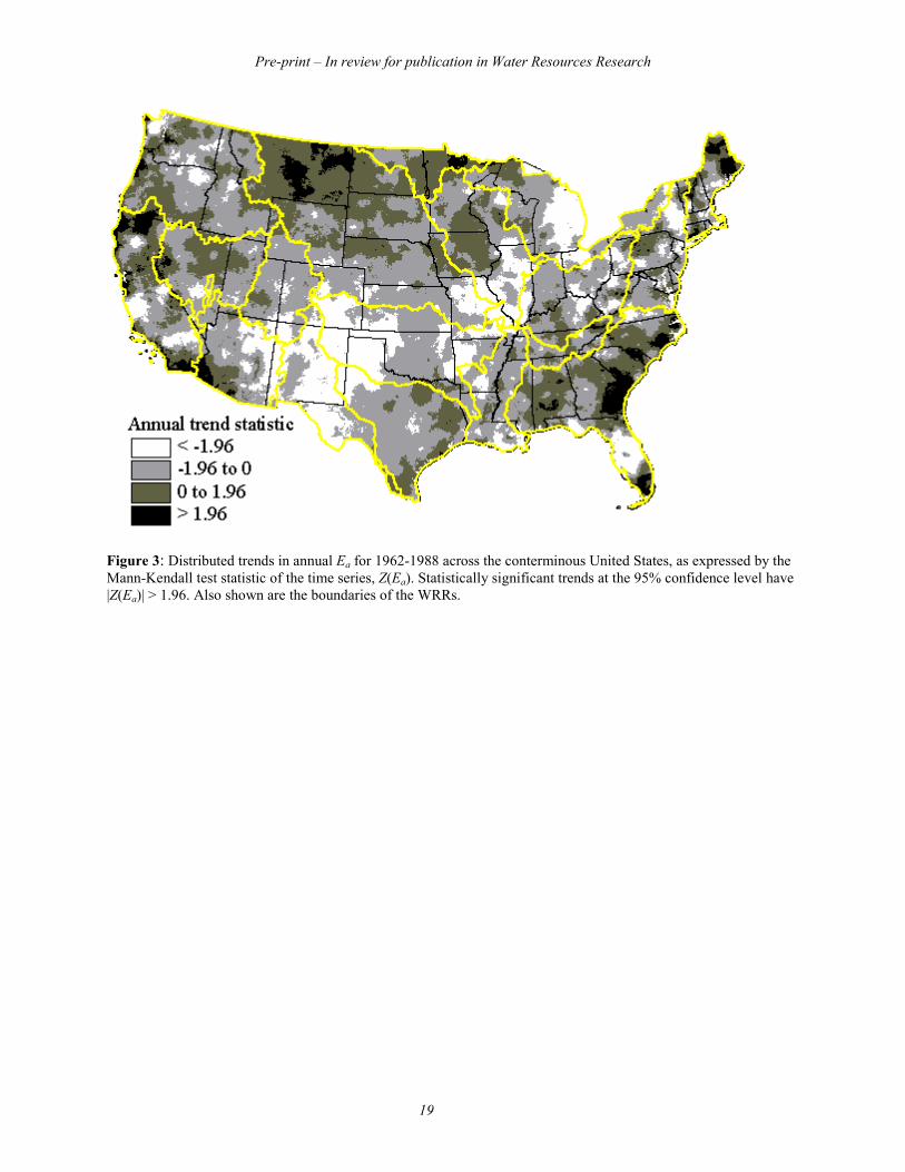
In the context of the complementary relationship, these two causes of trends in ETa�long-term changes in the degree of wetness of the basin i.e., ∆Ea, and long-term changes in the basin-wide net available energy, i.e., ∆Qn�may, for simplicity of analysis, be separated from each other, as demonstrated by the arrows marked �1� and �2� in Figure 1. The first cause�a long-term change in the drying power of the air (∆Ea) in the absence of a change in the energy budget�is akin to moving horizontally along the paired curves. As shown in equation (5), ETw is purely a function of the net available energy Qn. According to the complementary relationship and as shown in Figure 1, increasing the wetness of an evaporating surface (or decreasing the drying power of the air Ea) moves it to the right along both ETa and ETp, towards convergence of their respective curves, while decreasing wetness moves it to the left, towards divergence of the curves. This is shown by the arrow marked �1� in Figure 1. This dynamic may be indicated by the Mann-Kendall test statistic for the Ea time series, Z(Ea): if, for a particular basin, Z(Ea) is negative, then the basin is becoming wetter from the first effect; drier for a positive Z(Ea). The spatial distribution of Z(Ea) is shown in Figure 3.

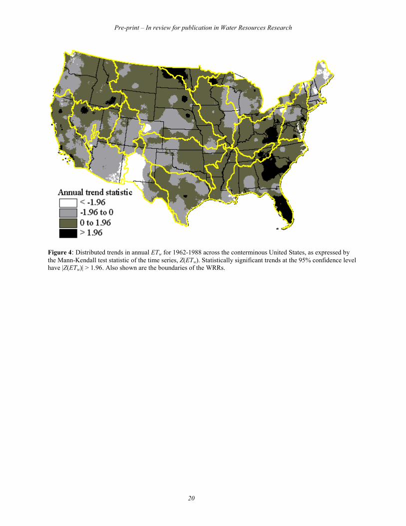
The second cause�a change in the long-term net available energy (∆Qn) in the absence of a change in wetness�shifts both the horizontal line representing ETw and the curve representing ETp upwards, in the case of increasing Qn, or downwards in the case of decreasing Qn. Correspondingly, and in accordance with the complementary relationship, the curve representing ETa will also shift in a similar direction, as shown by the arrow marked �2� in Figure 1. As ETw is a function of Qn only (see equation (5)), trends in the net available energy may be tracked with


10

the value of the Mann-Kendall test statistic for ETw, Z(ETw). The spatial distribution of Z(ETw) is shown in Figure 4.

It is important to recognize that, physically, these dynamics cannot be taken in isolation, but instead occur within the framework of complex feedback mechanisms beyond those that underpin the complementary relationship as it is currently formulated. For instance, the effect of a long-term decrease in the radiative budget, indicated here by a negative Z(ETw) value, may be an increase in soil moisture and thereby a decrease in the vapor pressure deficit of the over-passing air, which leads, in turn, to a lowering of the drying power of the air, and hence a negative Z(Ea). Next, we examine these possibilities in one WRR. WRR-scale analysis – Rio Grande basin

Here we report results for WRR 13 (the Rio Grande basin), an arid/semi-arid and topographically heterogeneous WRR, which is a combination that most challenges our model. The trend in annual ETa was calculated on a lumped basis at the WRR-scale, by spatially averaging annual ETa over the extent of the WRR, and annual ETa was observed to increase by 12.5% over our 27-year period, a trend that was significant at the 88.6% level. Figure 5 presents the distribution of annual ETa trends across the WRR and may be summarized by area, as follows: 0.2% shows annual ETa decreasing significantly (at the 95% level); 20.4% shows statistically insignificant decreasing ETa; 36.9% shows statistically insignificant increasing ETa; and 42.6% shows statistically significant (at the 95% level) increasing ETa .

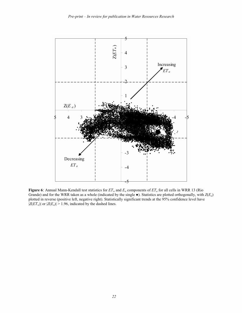
Figure 6 indicates, for each 5 km x 5 km cell in WRR 13 and for the WRR taken as a whole, the relative trends in the driving factors behind trends in ETa. The y-axis, Z(ETw), represents trends in the net available energy; increasing above the x-axis and decreasing below. The x-axis, Z(Ea), represents trends in the drying power of the air; increasing Ea and hence decreasing ETa to the left of the y-axis, and decreasing Ea and hence increasing ETa to the right. The axes are shown in this manner in order to correspond to the trends indicated in Figure 1, wherein the first cause for a trend in ETa�a trend in the net available energy�moves a cell vertically, and the second cause�a trend in the drying power of the air�moves a cell horizontally. Thus, each quadrant of Figure 6 represents a different combination of influences driving trends in ETa. As regards the trends in the components spatially averaged across WRR 13 as a whole, indicated by a large ● in Figure 6, decreasing trends are observed in both Ea (Z(Ea) = -2.79, statistically significant at the 99.5% level) and in ETw (Z(ETw) = -1.54, statistically significant at the 87.7% level). That the resulting trend in basinwide ETa is increasing indicates that of these conflicting effects on trends in ETa, the decreasing trend in Ea is more powerful than that in ETw. In physical terms, the decrease in ETa due to a long-term decrease in the net energy available for evaporation Qn (indicated here by ETw, as shown in (5)) is more than counteracted by the increase in ETa observed as a long-term reduction in wind speeds or in vapor pressure deficit due to basin wetting, or both.

With regard to the spatially distributed values in the 5 km x 5km pixels, cells in the upper-right quadrant are experiencing increasing ETw and decreasing Ea, a combination that increases ETa. These areas are indicated as cells that are simultaneously positive in Figure 4 and negative in Figure 3, and constitute a subset of the positive cells in Figure 5. Cells in the lower-left quadrant correspond to the opposite effects in both ETw and Ea, thus indicating a decreasing trend in ETa, and constitute a subset of the negative cells in Figure 5. The other two quadrants indicate


11

mixed effects on ETa; with ETw and Ea both increasing or both decreasing. Cells in these quadrants are represented as the remaining positive or negative pixels in Figure 5.

The spatial distribution of these orthogonal contributing trends can be derived from Figure 3 and Figure 4 and their effects in Figure 5. Those cells that, from Figure 6, we can predict are decreasing in ETa (those in the bottom left quadrant) are the areas along the lower reaches of the basin, in southern Texas. The cells in the top-right quadrant of Figure 6 lie in the far northern reaches of the WRR�the San Luis Valley, the eastern San Juan and western Sangre de Cristo mountain ranges in southern Colorado�and areas in western Texas and far southeastern New Mexico. The rest of the WRR is subject to conflicting trends in these two factors: either drying but with increasing net available energy (e.g., receiving more solar radiation), or wetting but with decreasing net available energy. Basin-scale analysis – Rio Puerco basin

To demonstrate the spatio-temporal flexibility of this analysis we turn to an even smaller spatial scale, that of a basin of approximately 16,000 km2 contained entirely within the WRR just examined, and to a monthly time step. This basin, the Rio Puerco in the arid Southwest, is well-metered and hydrologically at the soil-controlled end of the spectrum, where the performance of the Advection-Aridity model is stretched.

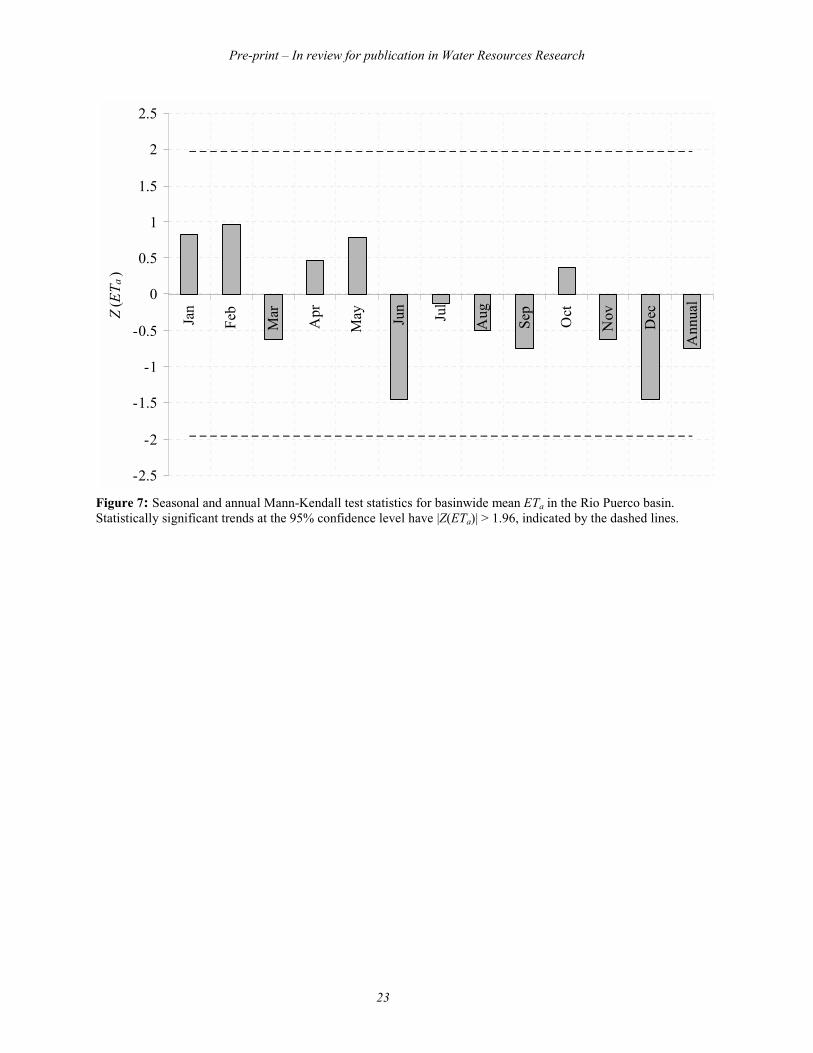
The seasonal and annual trends in ETa for the Rio Puerco basin as a whole over the 27-year period of this study are shown in Figure 7. On a seasonal basis, the decreasing ETa trends occur throughout the summer, fall and early winter months (June through December, except for October)�a period that includes the months of the highest mean ETa (June at 73 mm, and August at 74 mm). Through the winter and spring months (January through May, except for March), ETa appears to be increasing. On an annual basis, there is a decreasing trend. However, none of these trends was found to be significant at the 95% level.

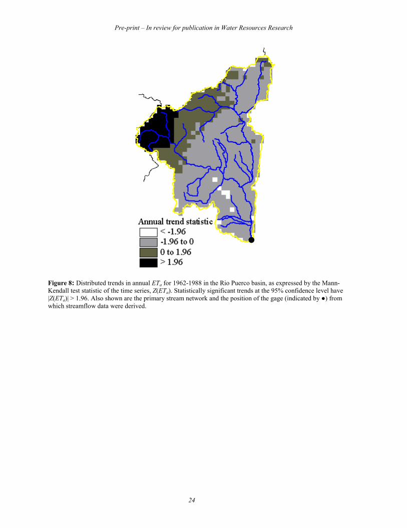
Figure 8 presents the spatial distribution of the annual trend statistic for the ETa time-series in the Rio Puerco basin and may be summarized by area, as follows: 0.9% shows statistically significant decreasing ETa; 67.8% shows statistically insignificant decreases in ETa; 21.8% shows statistically insignificant increases in ETa; and 9.4% shows statistically significant increases in ETa. By making use of the spatio-temporal flexibility of our model, more subtle and significant results may be extracted than is possible when the complementary relationship is applied to generate station values of ETa that are then spatially averaged at the continental scale (as in Szilagyi [2001] and Szilagyi et al. [2001]). Here, we see that while there are no significant seasonal or annual trends in ETa when it is examined at the basin-scale (see Figure 7), there are regions of the basin where there are indeed significant annual trends, specifically the uppermost, western reaches of the basin where ETa was increasing, and some regions in the lower reaches of the basin (near the outlet), where ETa was decreasing. That such fine detail and important findings get washed out when the distributed data are lumped, even over a relatively small basin, demonstrates the value of the spatially distributed approach. 6. DISCUSSION

In the study of climate change and/or variability it is essential first to establish a base-line for such modeling by rigorously examining past change and/or variability, and here we propose a methodology to address this need and report the findings of a study of trends in ETa at different spatial and temporal scales. A complementary relationship model, specifically the regional-seasonal Advection-Aridity model, was used to create the first ETa dataset of its kind�one that is spatially distributed, long-term (27 years), large-scale (continental), and checked across


12

hundreds of climatically and topographically diverse basins to maximize its climatological robustness. Distributed surfaces of these trends were produced and examined, first over the spatial extent of the data set and then over a particular WRR within it. Further, for a basin within this WRR, intra-annual trends were derived and these results were compared to existing work on precipitation and streamflow. Such a spatially distributed study of trends in ETa allows examination of sensitivities to climate change and variability at a wide variety of scales, from a continent to a single pixel. Further, examining long-term trends in the input climatic variables allows us to avoid assumptions of stationarity in any component of ETa. The primary contributions of this study are then three-fold:

(1) With regard to the ETa-estimation procedure, while many researchers have resorted to the use of ETpan observations as �perfect estimators� of ETp, which is supported by the complementary relationship hypothesis�at a point in a homogeneous region, the hypothesis indicates that a free-water surface will evaporate at the potential rate ETp�it is, in practice, a fundamentally flawed correspondence [Hobbins et al., 2001b]. In using ETpan observations in a trend analysis of ETa, one may inadvertently mis-diagnose the simple effects of local changes, such as urbanization, irrigation, or deforestation, as long-term climatological trends on a regional scale. However, in our use of the ETa time-series developed and tested by Hobbins et al. [2001a, 2001b], there is no reliance on station values of ETa to estimate regional or continental averages, nor on any ETpan-based approximation for ETp.

(2) With regard to the spatial characteristics and flexibility of the time-series, the complementary relationship is applied over as diverse a climatic and topographic extent as the conterminous United States, breaking the mold of previous studies that have either been conducted at small spatial scales, or at single sites. Furthermore, the spatially distributed nature of the ETa time-series allows for trends to be summarized at any scale and spatial breakdown, including the entire conterminous United States, WRRs, states, climatic divisions, specific watersheds, or physiographic regions. Spatially averaging our distributed ETa dataset at the continental scale over our 27-year period, we observed a 4.3% increase in annual ETa (statistically significant at the 90% confidence level), while over the smaller Rio Grande WRR we observed a 12.5% increase in annual ETa (statistically significant at the 88.6% confidence level). Averaging over the much smaller Rio Puerco basin did not produce a significant trend in ETa, but examination of individual pixels showed areas of significant trends. In general, and particularly on a spatially distributed basis, decreasing the spatial scope of analysis from the continental-scale through the WRR-scale to the basin- and subbasin-scale allowed for the clearer identification of areas with significant trends in ETa. Thus, the primary advantage of the application of the complementary relationship on a distributed basis was highlighted: that analysis is possible and useful results may be extracted at any scale, from the largest extent of analysis (the entire lower 48 states, in this case), to the smallest: that of a single pixel.

Dividing spatially along the lines of the smaller WRR-scale may yield too coarse a taxonomy. This conclusion is supported by Lins [1997] who, in a study of streamflow patterns and hydroclimatology at WRR-scales, concluded that while the division of the conterminous United States into the 18 WRRs as promulgated in 1970 by the Water Resources Council is based purely on surface watersheds, they do not correspond to observed hydroclimatology, as many of the hydrologic driving forces are not constrained by the drainage divides that define the WRRs. Generally, more meaningful conclusions may be derived by use of improved taxonomies; for example, by sub-dividing the WRRs into their component 4-digit hydrologic units, or using the 344 state climatic divisions.


13

(3) Trends in ETa are broken down into its climatic components in the context of the complementary relationship. Previous work by Szilagyi et al. [2001] explicitly assumed temporal stationarity of the net energy available at the surface for evaporation Qn, and specifically that d<ETw>/dt = 0, leaving only long-term trends in Ea�through either the vapor pressure deficit or the wind speed�to account for trends in ETa. Clearly, any long-term change in the energy available at the ground surface for evaporation (Qn) would necessarily result from changes in cloudiness, or in surface albedo and lead to changes in ETw and, therefore, in ETa. As they infer, their methodological assumption may more simply explain the difference between their watershed-based and complementary relationship-based ETa-trend estimates, leading their application of the complementary relationship systematically to overestimate such trends. Here, by making no assumptions about the temporal stationarity of cloudiness or surface albedo or, more precisely, of the net energy available at the surface for evaporation Qn, we have instead reported trends in both of these primary components of ETa.

Dividing ETa trends up as to their component origins may be a useful tool to determine effects of various climatological trends on ETa. Here, while the trends were derived and categorized as to their origins within the context of the driving forces of ETa�long-term changes in the degree of wetness of the basin and long-term changes in the basinwide available energy budget�no attempt was made to explain these trends on a climatological basis. Nor were other studies, such as ecological, land-use, or climate studies, examined for similarity of results. This type of diagnostic analysis is the subject of ongoing study.

Work is also underway to examine the ETa trends with respect to the input data�specifically temperature, humidity, and available energy�and, in selected basins where such data are available, to compare these trends to trends in other components of the surface hydrologic cycle, namely precipitation and streamflow. Such a comparison to previously reported trends in precipitation and streamflow at a basin- and seasonal-scale in a climatically challenging region demonstrated the climatic, spatial, and temporal flexibility of this application of the Advection-Aridity model to the examination of long-term trends in ETa. Further, the ETa trend data should be directly comparable to data from other branches of the science�models of land-use, ecological dynamics, or global circulation, for instance.

The regional-seasonal Advection-Aridity model is offered as a tool for studies of climate change and variability. Using the methodologies summarized in this paper, it is possible to examine trends in ETa and its components in any and all basins across the conterminous United States, as the input data are distributed and reflect surface conditions regardless of the origins of the water and degree of anthropogenic disturbance. It should be noted that work continues in this regard on a regional estimation of k-values (the complementary relationship constant shown in equation 1) in sub-optimal regions, and on quantifying the sources of the trends in ETa as they relate to its components, Ea and Qn. Improved estimates of the trends thus generated will be published when the work is complete. ACKNOWLEDGMENTS

This work was partially supported by the US Forest Service and the National Institute for Global Environmental Change through the U.S. Department of Energy (Cooperative Agreement No. DE-FC03-90ER61010). REFERENCES


14

Allen, R. G., 1986: A Penman for all seasons. Journal of Irrigation and Drainage Engineering, 112(4): 348�368.

Bouchet, R. J., 1963: Évapotranspiration réelle et potentielle, signification climatique. International Association Scientific Hydrology, Proceedings, Berkeley, California, U.S.A., Symp., Publ. No. 62: 134�142.

Brutsaert, W., and H. Stricker, 1979: An advection-aridity approach to estimate actual regional evapotranspiration. Water Resources Research, 15(2): 443�450.

Chiew, F. H. S., and T. A. McMahon, 1996: Trends in historical streamflow records. Regional Hydrological Response to Climate Change, J. A. A. Jones et al., Ed., Kluwer Academic Publishers, Amsterdam: 63�68.

DeBruin, H. A. R. and J. Q. Keijman, 1979: Priestley-Taylor evaporation model applied to a large, shallow lake in the Netherlands. Journal of Applied Meteorology, 18(7): 898�903.

Eagleson, P. S., 1978: Climate, soil and vegetation: 7. A derived distribution of annual water yield. Water Resources Research, 14(5): 765�776.

EarthInfo, 1998a: NCDC Summary of the Day [TD-3200 computer file]. Boulder, Colorado, U.S.A.

EarthInfo, 1998b: NCDC Surface Airways [TD-3280 computer file]. Boulder, Colorado, U.S.A. Gutman, G., 1988: A simple method for estimating monthly mean albedo from AVHRR data.

Journal of Applied Meteorology, 27(9): 973�988. Hobbins, M. T., J. A. Ramírez, and T. C. Brown, 1999: The complementary relationship in

regional evapotranspiration: the CRAE model and the Advection-Aridity approach. Proc. Nineteenth Annual A.G.U. Hydrology Days: 199�212.

Hobbins, M. T., J. A. Ramírez, T. C. Brown, and L. H. J. M. Claessens, 2001a: The complementary relationship in estimation of regional evapotranspiration: the CRAE and Advection-Aridity models. Water Resources Research, 37(5): 1367�1388.

Hobbins, M. T., J. A. Ramírez, and T. C. Brown, 2001b: The complementary relationship in estimation of regional evapotranspiration: an enhanced Advection-Aridity model. Water Resources Research, 37(5): 1389�1404.

Hobbins, M. T., J. A. Ramírez, and T. C. Brown, 2001c: Trends in regional evapotranspiration across the United States under the complementary relationship hypothesis. Proceedings of the Twenty-first Annual American Geophysical Union Hydrology Days: Colorado State University, Fort Collins, Colorado, U.S.A.: 106�121.

Karl, T. R. and R. W. Knight, 1998: Secular trends of precipitation amount, frequency, and intensity in the United States. Bulletin of the American Meteorological Society, 79(2): 231�241.

Karl, T. R., R. W. Knight, D. R. Easterling, and R. G. Quayle, 1996: Indices of climate change for the United States. Bulletin of the American Meteorological Society, 77(2): 279�292.

Katul, G. G., and M. B. Parlange, 1992: A Penman-Brutsaert model for wet surface evaporation. Water Resources Research, 28(1): 121�126.

Lettenmaier, D. P., E. F. Wood, and J. R. Wallis, 1994: Hydro-climatological trends in the continental United States, 1948�88. Journal of Climate, 7: 586�607.

Lins, H. F., 1997: Regional streamflow regimes and hydroclimatology of the United States. Water Resources Research, 33(2): 1655�1667.

Lins, H. F. and J. R. Slack, 1999: Streamflow trends in the United States. Geophysical Research Letters, 26(2): 227�230.


15

Lockwood, J. G., 1994: Climatic change, grass pasture and potential evapotranspiration. Weather, 49(9): 318�321.

McNaughton, K. G., and T. A. Black, 1973: Study of evapotranspiration from a Douglas-Fir forest using energy-balance approach. Water Resources Research, 9(6): 1579�1590.

Molnár, P., and J. A. Ramírez, 2001: Recent trends in precipitation and streamflow in the Rio Puerco basin. Journal of Climate, 14: 2317�2328.

Morton, F. I., 1965: Potential evaporation and river basin evaporation. ASCE Journal of the Hydraulics Division, ASCE, 91(HY6): 67�97.

Morton, F. I., 1975: Estimating evaporation and transpiration from climatological observations, Journal of Applied Meteorology, 14: 488�497.

Morton, F. I.,, 1976a: Climatological estimates of evapotranspiration, ASCE Journal of the Hydraulics Division, 102(HY3): 275�291.

Morton, F. I., 1976b: Climatological estimates of lake evaporation, Water Resources Research, 15(1): 64�76.

Morton, F. I., 1978: Estimating evapotranspiration from potential evaporation: Practicality of an iconoclastic approach. Journal of Hydrology, 38: 1�32.

Morton, F. I., 1983: Operational estimates of areal evapotranspiration and their significance to the science and practice of hydrology. Journal of Hydrology, 66: 1�76.

National Oceanic and Atmospheric Administration (NOAA), 1993: Solar and Meteorological Surface Observation Network 1961-1990 (CD-ROM), Version 1.0. National Climatic Data Center, EDIS, Federal Building, Asheville, NC.

Parlange, M. B., and G. G. Katul, 1992a: Estimation of the diurnal variation of potential evaporation from a wet bare soil surface. Journal of Hydrology, 132: 71�89.

Parlange, M. B., and G. G. Katul, 1992b: An advection-aridity evaporation model. Water Resources Research, 28(1): 127�132.

Penman, H. L., 1948: Natural evaporation from open water, bare soil and grass. Proceedings of the Royal Society of London, Series A., 193: 120�146.

Peterson, T. C., V. S. Golubev, and P. Y. Groisman, 1995: Evaporation losing its strength. Nature, 377, 687�688.

Priestley, C. H .B., and R. J. Taylor, 1972: On the assessment of surface heat flux and evaporation using large-scale parameters. Monthly Weather Review, 100: 81�92.

Szilagyi, J., 2001: Modeled Areal Evaporation Trends over the Conterminous United States. Journal of Irrigation Drainage and Engineering. July/August, 196�200.

Szilagyi, J., G. G. Katul, and M. B. Parlange, 2001: Evapotranspiration Intensifies over the Conterminous United States. Journal of Water Resources Planning and Management. 127(6), 354�362.

Van Bavel, C. H. M., 1966: Potential evaporation: the combination concept and its experimental verification. Water Resources Research, 2(3): 455�467.

Wahl, K. L., 1992: Evaluation of trends in runoff in the western United States. Proceedings, Managing Water Resources During Global Change, 28th Annual Conference and Symposium, Reno, NV, American Water Resources Association, 701�710.

Westmacott, J. R., and D. H. Burn, 1997: Climate change effects on the hydrologic regime within the Churchill-Nelson River Basin. Journal of Hydrology, 202: 263�279.

Wright, J. L., 1982: New evapotranspiration crop coefficients. Journal of Irrigation and Drainage Division, ASCE, 108(IR2): 57�74.


16

List of Figures Figure 1: Schematic representation of the complementary relationship in regional evapotranspiration. Arrows marked �1� and �2� indicate the effects on ETa of trends in its Ea and ETw components, respectively, in the context of the complementary relationship. Figure 2: Distributed trends in annual ETa for 1962-1988 across the conterminous United States, as expressed by the Mann-Kendall test statistic of the time series, Z(ETa). Statistically significant trends at the 95% confidence level have |Z(ETa)| > 1.96. Also shown are the boundaries, numbers, and names of the WRRs. Figure 3: Distributed trends in annual Ea for 1962-1988 across the conterminous United States, as expressed by the Mann-Kendall test statistic of the time series, Z(Ea). Statistically significant trends at the 95% confidence level have |Z(Ea)| > 1.96. Also shown are the boundaries of the WRRs. Figure 4: Distributed trends in annual ETw for 1962-1988 across the conterminous United States, as expressed by the Mann-Kendall test statistic of the time series, Z(ETw). Statistically significant trends at the 95% confidence level have |Z(ETw)| > 1.96. Also shown are the boundaries of the WRRs. Figure 5: Distributed trends in annual ETa for 1962-1988 in WRR 13 (Rio Grande), as expressed by the Mann-Kendall test statistic of the time series, Z(ETa). Statistically significant trends at the 95% confidence level have |Z(ETa)| > 1.96. Also shown in white is the boundary of the Rio Puerco basin. Figure 6: Annual Mann-Kendall test statistics for ETw and Ea components of ETa for all cells in WRR 13 (Rio Grande) and for the WRR taken as a whole (indicated by the single ●). Statistics are plotted orthogonally, with Z(Ea) plotted in reverse (positive left, negative right). Statistically significant trends at the 95% confidence level have |Z(ETw)| or |Z(Ea)| > 1.96, indicated by the dashed lines. Figure 7: Seasonal and annual Mann-Kendall test statistics for basinwide mean ETa in the Rio Puerco basin. Statistically significant trends at the 95% confidence level have |Z(ETa)| > 1.96, indicated by the dashed lines. Figure 8: Distributed trends in annual ETa for 1962-1988 in the Rio Puerco basin, as expressed by the Mann-Kendall test statistic of the time series, Z(ETa). Statistically significant trends at the 95% confidence level have |Z(ETa)| > 1.96. Also shown are the primary stream network and the position of the gage (indicated by ●) from which streamflow data were derived.


17

Figure 1: Schematic representation of the complementary relationship in regional evapotranspiration. Arrows marked �1� and �2� indicate the effects on ETa of trends in its Ea and ETw components, respectively, in the context of the complementary relationship.

Rat

es

Increasing moisture availability

ETa

ETp

ETw

� 1

2


18

Water Resource Regions (WRRs) 1 New England 2 Mid-Atlantic 3 South Atlantic-Gulf 4 Great Lakes 5 Ohio 6 Tennessee 7 Upper Mississippi 8 Lower Mississippi 9 Souris-Red-Rainy

10 Missouri 11 Arkansas-White-Red 12 Texas-Gulf 13 Rio Grande 14 Upper Colorado 15 Lower Colorado 16 Great Basin 17 Pacific Northwest 18 California

Figure 2: Distributed trends in annual ETa for 1962-1988 across the conterminous United States, as expressed by the Mann-Kendall test statistic of the time series, Z(ETa). Statistically significant trends at the 95% confidence level have |Z(ETa)| > 1.96. Also shown are the boundaries, numbers, and names of the WRRs.

17

214

15

16

13

12

11

910

7

8

6

1

18

3

4

5


19

Figure 3: Distributed trends in annual Ea for 1962-1988 across the conterminous United States, as expressed by the Mann-Kendall test statistic of the time series, Z(Ea). Statistically significant trends at the 95% confidence level have |Z(Ea)| > 1.96. Also shown are the boundaries of the WRRs.


20

Figure 4: Distributed trends in annual ETw for 1962-1988 across the conterminous United States, as expressed by the Mann-Kendall test statistic of the time series, Z(ETw). Statistically significant trends at the 95% confidence level have |Z(ETw)| > 1.96. Also shown are the boundaries of the WRRs.


21

Figure 5: Distributed trends in annual ETa for 1962-1988 in WRR 13 (Rio Grande), as expressed by the Mann-Kendall test statistic of the time series, Z(ETa). Statistically significant trends at the 95% confidence level have |Z(ETa)| > 1.96. Also shown in white is the boundary of the Rio Puerco basin.


22

-5

-4

-3

-2

-1

0

1

2

3

4

5

-5-4-3-2-1012345

Z(E a )

Z(ET

w)

IncreasingET a

DecreasingET a

Figure 6: Annual Mann-Kendall test statistics for ETw and Ea components of ETa for all cells in WRR 13 (Rio Grande) and for the WRR taken as a whole (indicated by the single ●). Statistics are plotted orthogonally, with Z(Ea) plotted in reverse (positive left, negative right). Statistically significant trends at the 95% confidence level have |Z(ETw)| or |Z(Ea)| > 1.96, indicated by the dashed lines.


23

-2.5

-2

-1.5

-1

-0.5

0

0.5

1

1.5

2

2.5

Jan

Feb

Mar

Apr

May Jun Jul

Aug

Sep

Oct

Nov Dec

Ann

ual

Z(E

T a)

Figure 7: Seasonal and annual Mann-Kendall test statistics for basinwide mean ETa in the Rio Puerco basin. Statistically significant trends at the 95% confidence level have |Z(ETa)| > 1.96, indicated by the dashed lines.


24

Figure 8: Distributed trends in annual ETa for 1962-1988 in the Rio Puerco basin, as expressed by the Mann-Kendall test statistic of the time series, Z(ETa). Statistically significant trends at the 95% confidence level have |Z(ETa)| > 1.96. Also shown are the primary stream network and the position of the gage (indicated by ●) from which streamflow data were derived.

�

Documents

TRENDS IN REGIONAL EVAPOTRANSPIRATION ACROSS THE …